Spatial Decision Tree: A Novel Approach to Land-Cover Classification

Zhe Jiang1, Shashi Shekhar1, Xun Zhou1, Joseph Knight2, Jennifer Corcoran2

1

1Department of Computer Science & Engineering 2Department of Forest Resources

University of Minnesota, Twin Cities

Highlights • Public engagement with science and technology :

– Coursera MOOC, “From GPS and Google Maps to Spatial Computing”, – reached 21,844 participants across 182 countries

• Enhanced infrastructure for education – Interdisciplinary survey paper on spatiotemporal change footprint discovery – Encyclopedia of GIS (Springer, 2nd Edition): Multiple articles on climate change – APA/IEEE Computing in Sc. & Eng. special issue on “Computing and Climate”

• Enhanced infrastructure for research – Spatial decision trees can help improve wetland maps for climate models

Highlights • Understanding

– Large semantic gap between Data Science and Climate Science • Data Science results are hard to interpret in Climate Science

– Data Science assumptions violate laws of physics • unnecessary errors, e.g., salt and pepper noise

• Concepts: – Physics-Guided Data Mining concepts are potentially transformative – Ex. Spatial Decision Trees: explicit physics (e.g., continuity) to wetland mapping – Ex. Intervals of Persistent Change detection uses Physics (e.g., violation of continuity)

Spatial Decision Tree: Motivation • Wetland mapping:

– Climate Change: wetlands – major source of methane1

– manage natural disasters, defense against hurricanes, buffer of floods. – maintain biodiversity, habitats to wildlife species

5 1Bryan Walsh, How Wetlands Worsen Climate Change, Time, Magazine, 2010

wildlife habitats Greenhouse Gas Methane flood control

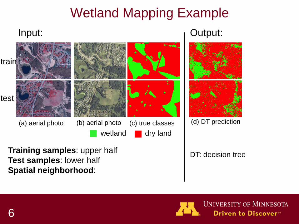
Wetland Mapping Example

(a) aerial photo (b) aerial photo (c) true classes (d) DT prediction

6

wetland dry land

Input: Output:

DT: decision tree Training samples: upper half

Test samples: lower half Spatial neighborhood:

train

test

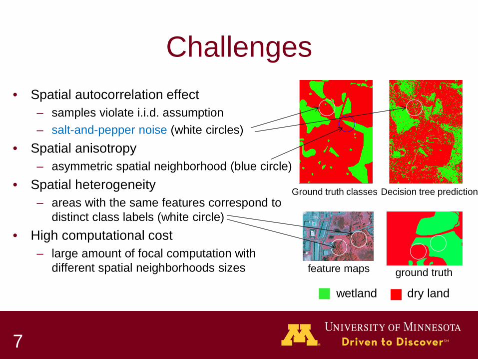
Challenges • Spatial autocorrelation effect

– samples violate i.i.d. assumption – salt-and-pepper noise (white circles)

• Spatial anisotropy – asymmetric spatial neighborhood (blue circle)

• Spatial heterogeneity – areas with the same features correspond to

distinct class labels (white circle) • High computational cost

– large amount of focal computation with different spatial neighborhoods sizes

7

Ground truth classes Decision tree prediction

ground truth feature maps

wetland dry land

Problem Statement • Given:

– training & test samples from a raster spatial framework – spatial neighborhood, its maximum size

• Find: – a (spatial) decision tree

• Objective: – minimize classification error and salt-and-pepper noise

• Constraint: – training samples are contiguous patches – spatial autocorrelation, anisotropy, and heterogeneity exist – training dataset can be large with high computational cost

8

9

Example with Decision Tree

ID f1 f2 class A 3 3 red B 3 3 red C 1 2 green D 3 1 red E 3 1 red F 3 1 red G 3 3 red H 1 2 green I 1 2 green J 3 1 red K 1 1 red L 3 1 red M 1 2 green N 1 2 green O 3 1 red P 3 1 red Q 3 1 red R 1 1 red

Input: Output:

In this example, Gamma index Γ1 on feature f1 is unique. Most often, Γ1 is computed on the fly.

decision tree

I

pixel id

M

C H

N

K A B

F G

D E

J L

Q R

O P

f1 ≤ 1

green red yes no

A B C D E F G H I J K L M N O P Q R

A B C D E F G H I J K L M N O P Q R

predicted map

salt-and-pepper noise pixel K from decision tree

R

Related Work Summary

10

Existing Work Proposed Work Tree local feature test &

information gain: focal feature test & spatial

information gain: Ensemble bootstrap sampling: geographic space partitioning:

single decision tree

ensemble of decision trees

traditional decision tree spatial decision tree

random forest ensemble spatial ensemble

Proposed Approach – Focal Test • Focal feature test

– Test both local and focal (neighborhood) information

– focal test uses local autocorrelation statistics, e.g., Gamma index

11

Local

Focal

Zonal

Proposed Approach - 2

12

where: i, j: pixel locations Si,j: similarity between location i and j Wi,j is adjacency matrix element

• tree traversal direction depends on both local and focal (neighborhood) information

• focal test uses local autocorrelation statistics, e.g., Gamma index (Γ)

• neighborhood

Example – Focal Tests

13

traditional decision tree spatial decision tree

inputs: table of records

adaptive neigh., 3 by 3

inputs: feature maps, class map

ID f1 f2 Γ1 class C 1 2 green H 1 2 green I 1 2 green K 1 1 red M 1 2 green N 1 2 green R 1 1 red A 3 3 red B 3 3 red D 3 1 red E 3 1 red F 3 1 red G 3 3 red J 3 1 red L 3 1 red O 3 1 red P 3 1 red Q 3 1 red

ID f1 f2 Γ1 class A 3 3 red B 3 3 red C 1 2 green D 3 1 red E 3 1 red F 3 1 red G 3 3 red H 1 2 green I 1 2 green J 3 1 red K 1 1 red L 3 1 red M 1 2 green N 1 2 green O 3 1 red P 3 1 red Q 3 1 red R 1 1 red

3 3 1 3 3 3 3 1 1 3 1 3 1 1 3 3 3 1

3 3 2 1 1 1 3 2 2 1 1 1 2 2 1 1 1 1

feature f1

feature f2

class map

1 1 1 1 1 1 1 1 1 1 -1 1 1 1 1 1 1 -1

focal function Γ1

pixel id A B C D E F G H I J K L M N O P Q R

3 3 1 3 3 3 3 1 1 3 1 3 1 1 3 3 3 1

f1 ≤ 1

green red yes no

I M

C H

N

K A B

F G

D E

J L

Q

R O P

( f1 ≤ 1 ) * (Γ1 ≥ 0)

green red + -

I M

C H

N

K A B

F G

D E

J

L

Q R

O P

A B C D E F G H I J K L M N O P Q R

predicted map

A B C D E F G H I J K L M N O P Q R

predicted map

ID f1 f2 Γ1 class C 1 2 1 green H 1 2 1 green I 1 2 1 green K 1 1 -1 red M 1 2 1 green N 1 2 1 green R 1 1 -1 red A 3 3 1 red B 3 3 1 red D 3 1 1 red E 3 1 1 red F 3 1 1 red G 3 3 1 red J 3 1 1 red L 3 1 1 red O 3 1 1 red P 3 1 1 red Q 3 1 1 red

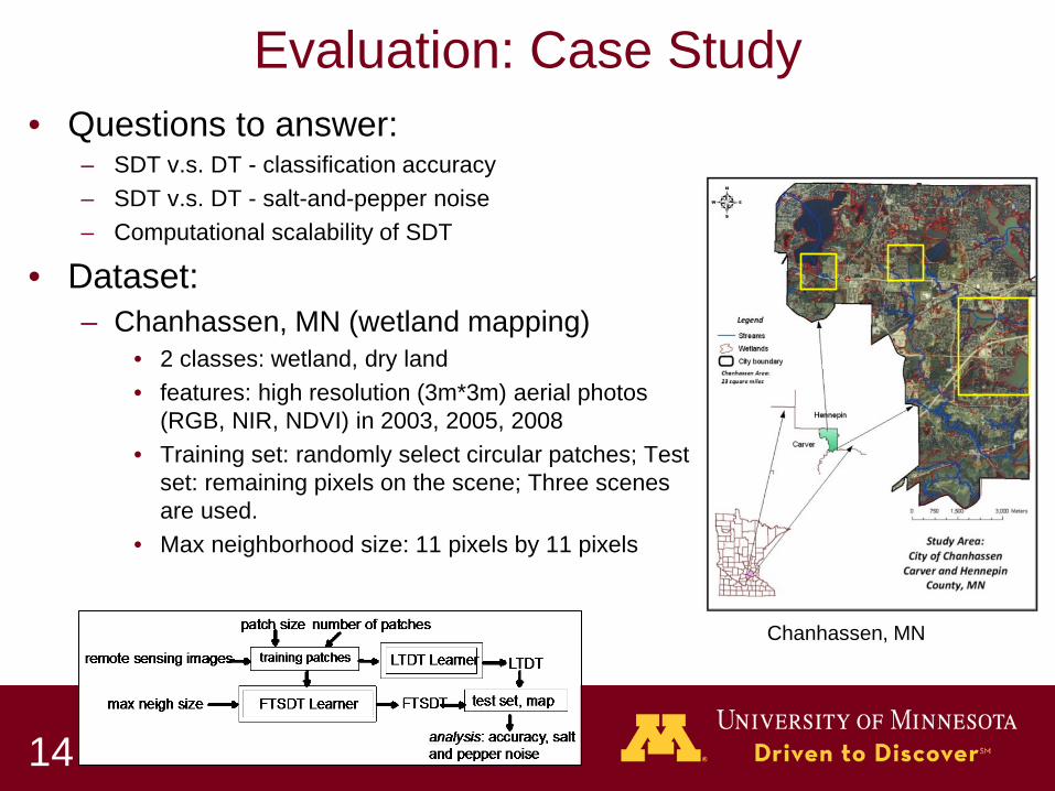
Evaluation: Case Study • Questions to answer:

– SDT v.s. DT - classification accuracy – SDT v.s. DT - salt-and-pepper noise – Computational scalability of SDT

• Dataset: – Chanhassen, MN (wetland mapping)

• 2 classes: wetland, dry land • features: high resolution (3m*3m) aerial photos

(RGB, NIR, NDVI) in 2003, 2005, 2008 • Training set: randomly select circular patches; Test

set: remaining pixels on the scene; Three scenes are used.

• Max neighborhood size: 11 pixels by 11 pixels

14

Chanhassen, MN

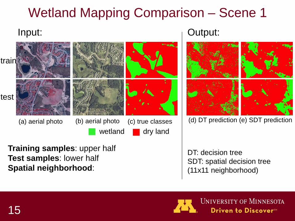
Wetland Mapping Comparison – Scene 1

(a) aerial photo (b) aerial photo (c) true classes (d) DT prediction

15

wetland dry land

Input: Output:

(e) SDT prediction

DT: decision tree SDT: spatial decision tree (11x11 neighborhood)

Training samples: upper half Test samples: lower half Spatial neighborhood:

train

test

decision tree (DT) spatial decision tree (SDT)

Trends: 1.DT: salt-and-pepper noise 2.SDT improve accuracy, salt-and-pepper noise levels

Classification Performance – Scene 2

true wetland true dryland false wetland false dryland

17

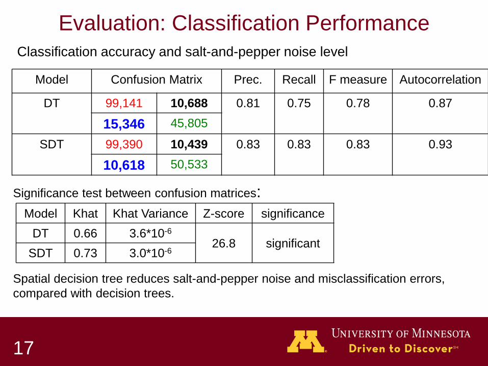
Evaluation: Classification Performance

Model Confusion Matrix Prec. Recall F measure Autocorrelation

DT 99,141 10,688 0.81 0.75 0.78 0.87

15,346 45,805

SDT 99,390 10,439 0.83 0.83 0.83 0.93

10,618 50,533

Model Khat Khat Variance Z-score significance DT 0.66 3.6*10-6

26.8 significant SDT 0.73 3.0*10-6

Classification accuracy and salt-and-pepper noise level

Significance test between confusion matrices:

Spatial decision tree reduces salt-and-pepper noise and misclassification errors, compared with decision trees.

Computational Bottleneck Analysis

18

Analysis: 1. focal computation takes the

vast majority of the time

2. focal computation cost increases faster with the training set size Focal computation is the bottleneck!

Incremental Update Approach

19

1 9 9 9 2 9 9 9 3 8 7 6 4 5 5 5

1 -1 -1 -1 -1 -1 -1 -1 -1 -1 -1 -1 -1 -1 -1 -1

-1 0.6 1 1

0.6 0.75 1 1

1 1 1 1

1 1 1 1

1 -1 -1 -1 1 -1 -1 -1 -1 -1 -1 -1 -1 -1 -1 -1

-0.33 0.2 1 1

-0.6 0.5 1 1

0.6 0.75 1 1

1 1 1 1

1 -1 -1 -1 1 -1 -1 -1 1 -1 -1 -1 -1 -1 -1 -1

-0.33 0.2 1 1

-0.2 0.25 1 1

-0.6 0.5 1 1

0.33 0.6 1 1

1 -1 -1 -1 1 -1 -1 -1 1 -1 -1 -1 1 -1 -1 -1

-0.33 0.2 1 1

-0.2 0.25 1 1

-0.2 0.25 1 1 -

0.33 0.2 1 1

(a) feature values (b) indicators, focal values for δ=1 (c) indicators, focal values for δ=2

(d) indicators, focal values for δ=3 (e) indicators, focal values for δ=4

candidate δ {1, 2, 3, 4, 5, 6, 7, 8}

Key idea: reduce redundant focal computation by reusing results across candidate test thresholds Γ(f < δ)

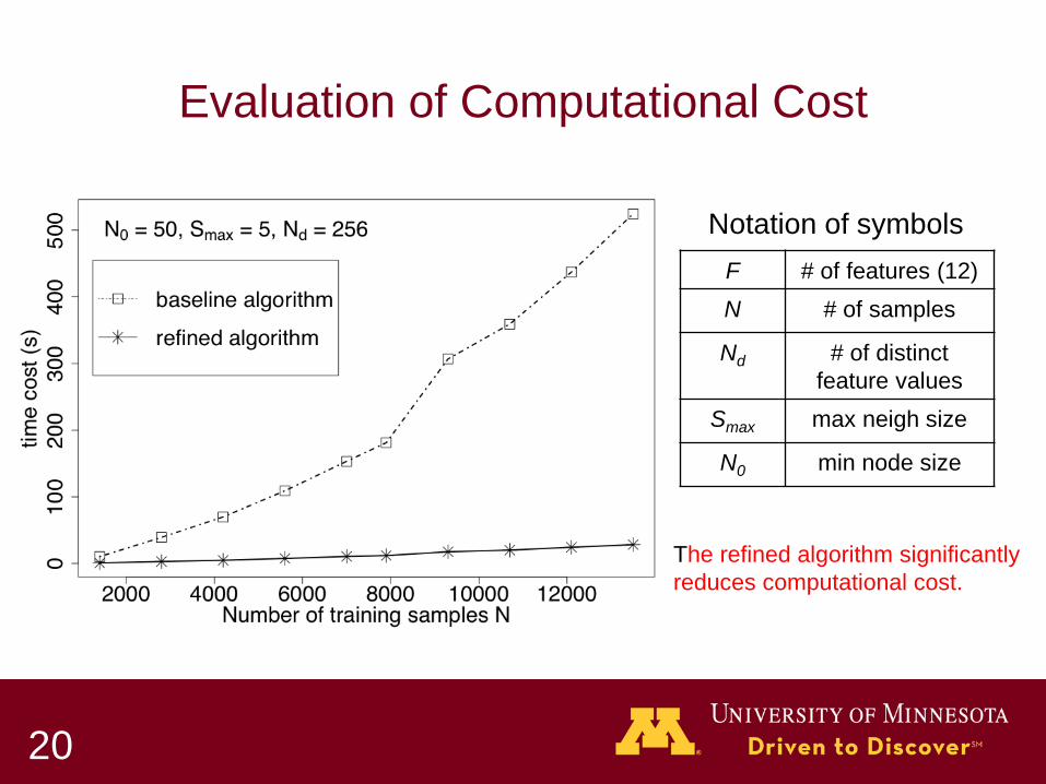
Evaluation of Computational Cost

20

The refined algorithm significantly reduces computational cost.

F # of features (12) N # of samples

Nd # of distinct feature values

Smax max neigh size

N0 min node size

Notation of symbols

Conclusions • Ignoring auto-correlation leads to errors, e.g., salt-n-pepper noise • Proposed a novel spatial decision tree approach with focal tests • Evaluation shows that proposed method reduced salt-n-pepper noise

– And improved classification accuracy

• Designed computational refinements to improve scalability

21

Publications on Spatial Decision Trees

[1] Z. Jiang, S. Shekhar, X. Zhou, J. Knight, J. Corcoran: Focal-Test-Based Spatial Decision Tree Learning. IEEE Transactions on Knowledge and Data Engineering (TKDE) 27(6): 1547-1559 (2015) [2] Z. Jiang, S. Shekhar, X. Zhou, J. Knight, J. Corcoran: Focal-Test-Based Spatial Decision Tree Learning: A Summary of Results. IEEE International Conference on Data Mining (ICDM) 2013: 320-329 [3] Z. Jiang, S. Shekhar, P. Mohan, J. Knight, and J. Corcoran. "Learning spatial decision tree for geographical classification: a summary of results.” International Conference on Advances in GIS, pp. 390-393. ACM, 2012. [4] Z. Jiang, S. Shekhar, A. Kamzin, and J. Knight. "Learning a Spatial Ensemble of Classifiers for Raster Classification: A Summary of Results.” IEEE International Conference on Data Mining Workshop, IEEE, 2014.

22

Challenges Revisited • Spatial autocorrelation effect

– samples violate i.i.d. assumption – salt-and-pepper noise (white circles)

• Spatial anisotropy – asymmetric spatial neighborhood (blue circle)

• Spatial heterogeneity – areas with the same features correspond to

distinct class labels (white circle) • High computational cost

– large amount of focal computation with different spatial neighborhoods sizes

23

Ground truth classes Decision tree prediction

ground truth feature maps

wetland dry land

Future Work • Key idea I: focal feature test

– tree traversal direction depends on both local and focal (neighborhood) information – focal test uses local autocorrelation statistics, e.g., Gamma index

• Key idea II: spatial information gain (SIG) – SIG = Info. Gain * α + Spatial Autocorrelation * (1 – α) – tree node test selection depends on both class purification and autocorrelation

structure

• Key idea III: spatial ensemble of local trees – geographic space partitioning, learn local classifiers

24

25

Proposed Approach: Spatial Ensemble traditional ensemble

(random forest) spatial ensemble

(spatial forest)

1. assume i.i.d. distribution 2. bootstrap sampling 3. learn a tree from one sampling with random feature subsets

1. assume spatial heterogeneity 2. spatial partitioning 3. learn local tree model in each partition

f1 ≤ 1

red green yes no

f1 ≤ 1

red green yes no

f1 ≤ 1

red green yes no

f1 ≤ 1

red green yes no

f1 ≤ 1

red green yes no

f1 ≤ 1

red green yes no

spatial ensemble single DT prediction ground truth

spatial cluster (islands)

partition P1 partition P2

one feature image ground truth

random forest

archipelagos

prediction in P1 prediction in P2

26