sparse mri -
TRANSCRIPT
Michael (Miki) LustigDepartment of Electrical Engineering and Computer Science, UC Berkeley
“Randomness is too important to be left to chance.”*
*R. Conveyo, Oak Ridge National Laboratory
Sparse MRI
M. Lustig, EECS UC Berkeley
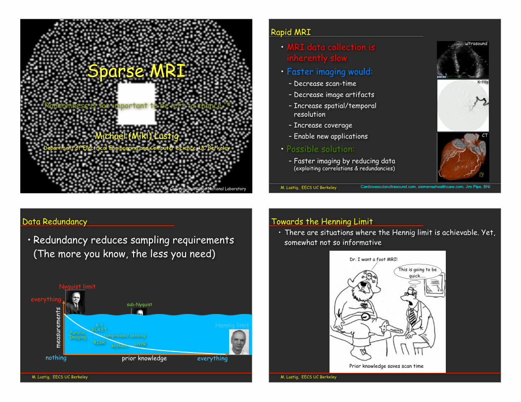
Rapid MRI
• MRI data collection is inherently slow
• Faster imaging would:– Decrease scan-time– Decrease image artifacts– Increase spatial/temporal
resolution– Increase coverage– Enable new applications
• Possible solution:– Faster imaging by reducing data
(exploiting correlations & redundancies)
ultrasound
x-ray
CT
Cardiovascularultrasound.com, siemensehealthcare.com, Jim Pipe, BNI
sub-Nyquist
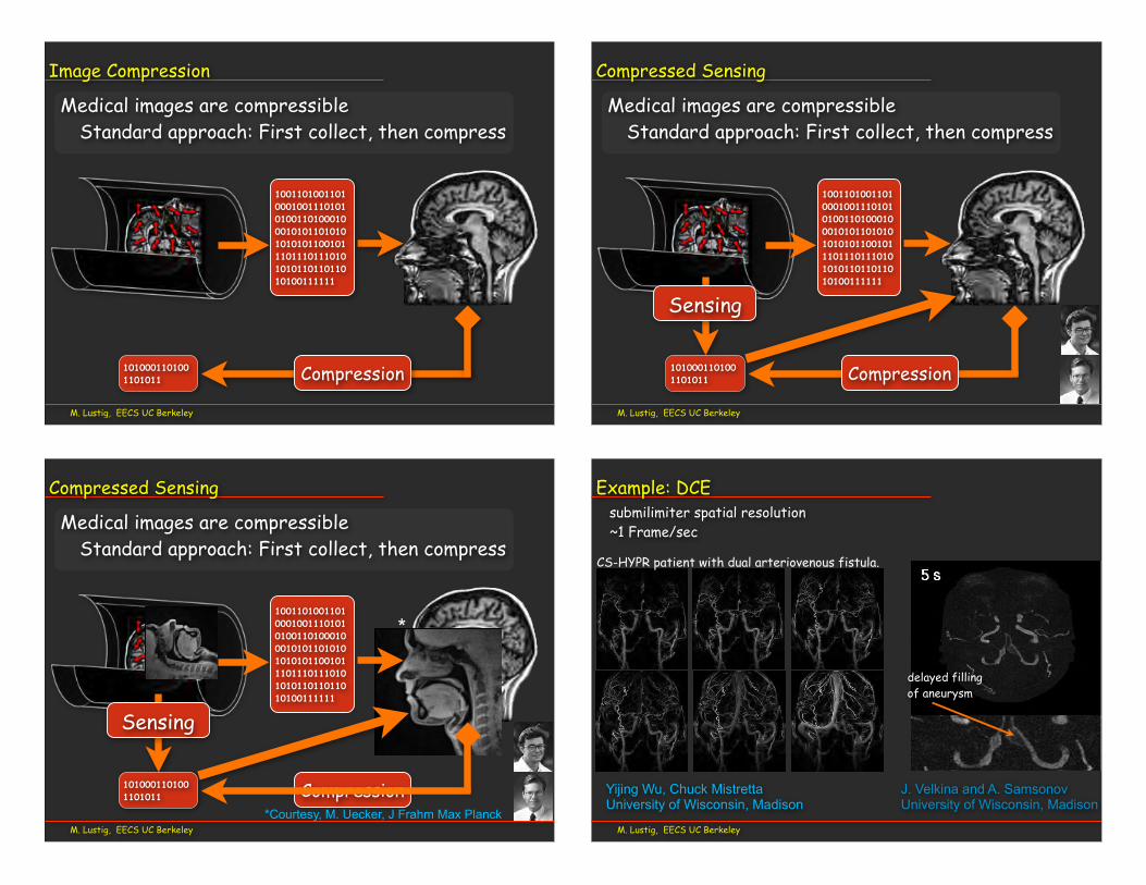
• Redundancy reduces sampling requirements(The more you know, the less you need)
Nyquist limit
M. Lustig, EECS UC Berkeley
Data Redundancy
prior knowledge everything
Hennig limit
everything
nothing
mea
sure
men
ts
ParallelImaging
k-tBLAST
RIGRkeyhole
compressed sensing
HYPR
M. Lustig, EECS UC Berkeley
Towards the Henning Limit• There are situations where the Hennig limit is achievable. Yet,
somewhat not so informative
Prior knowledge saves scan time
Dr. I want a foot MRI!
This is going to bequick.....
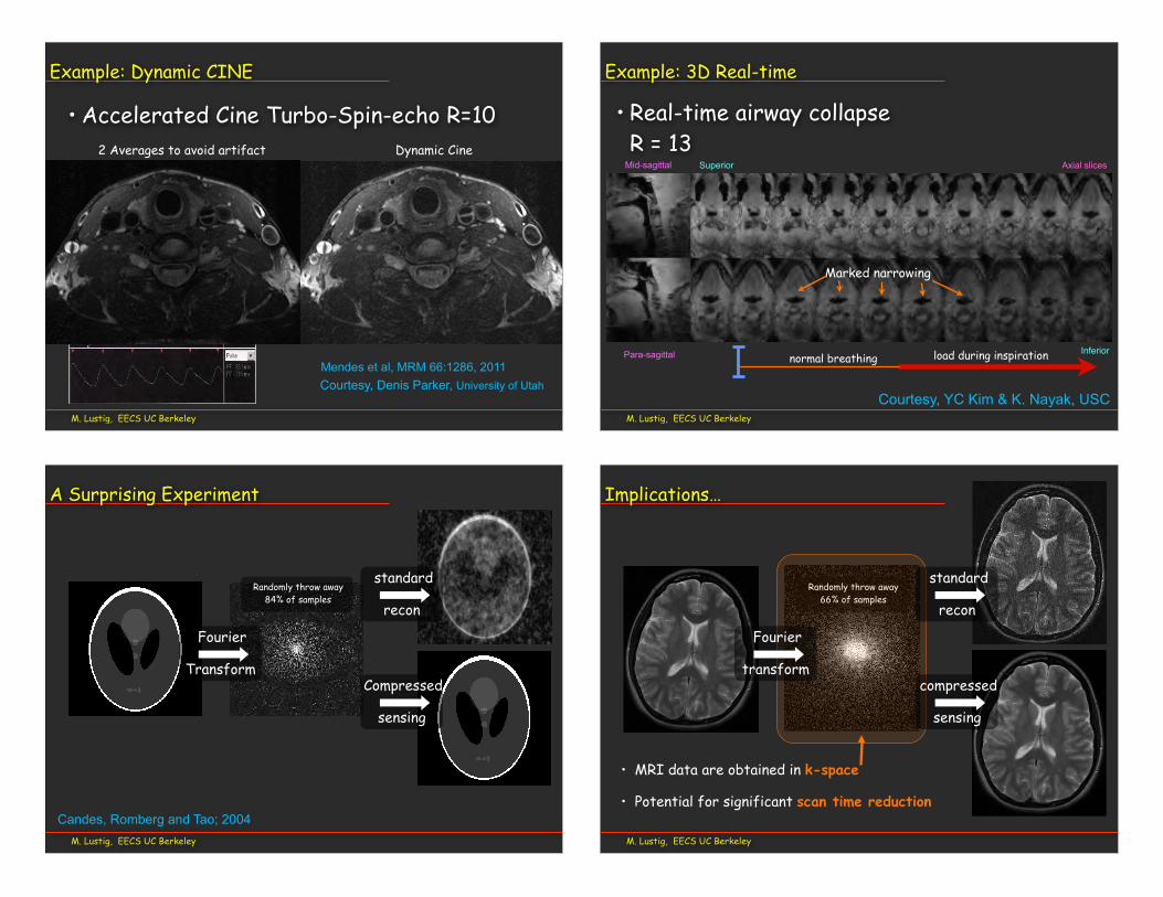
Medical images are compressibleStandard approach: First collect, then compress
M. Lustig, EECS UC Berkeley
Image Compression
100110100110100010011101010100110100010001010110101010101011001011101110111010101011011011010100111111
1010001101001101011 Compression
Medical images are compressibleStandard approach: First collect, then compress
M. Lustig, EECS UC Berkeley
Compressed Sensing
100110100110100010011101010100110100010001010110101010101011001011101110111010101011011011010100111111
1010001101001101011 Compression
Sensing
Medical images are compressibleStandard approach: First collect, then compress
M. Lustig, EECS UC Berkeley
Compressed Sensing
100110100110100010011101010100110100010001010110101010101011001011101110111010101011011011010100111111
1010001101001101011 Compression
Sensing
*Courtesy, M. Uecker, J Frahm Max Planck
*
M. Lustig, EECS UC Berkeley
Example: DCE
delayed filling of aneurysm
J. Velkina and A. SamsonovUniversity of Wisconsin, Madison
Yijing Wu, Chuck MistrettaUniversity of Wisconsin, Madison
submilimiter spatial resolution~1 Frame/sec
CS-HYPR patient with dual arteriovenous fistula.
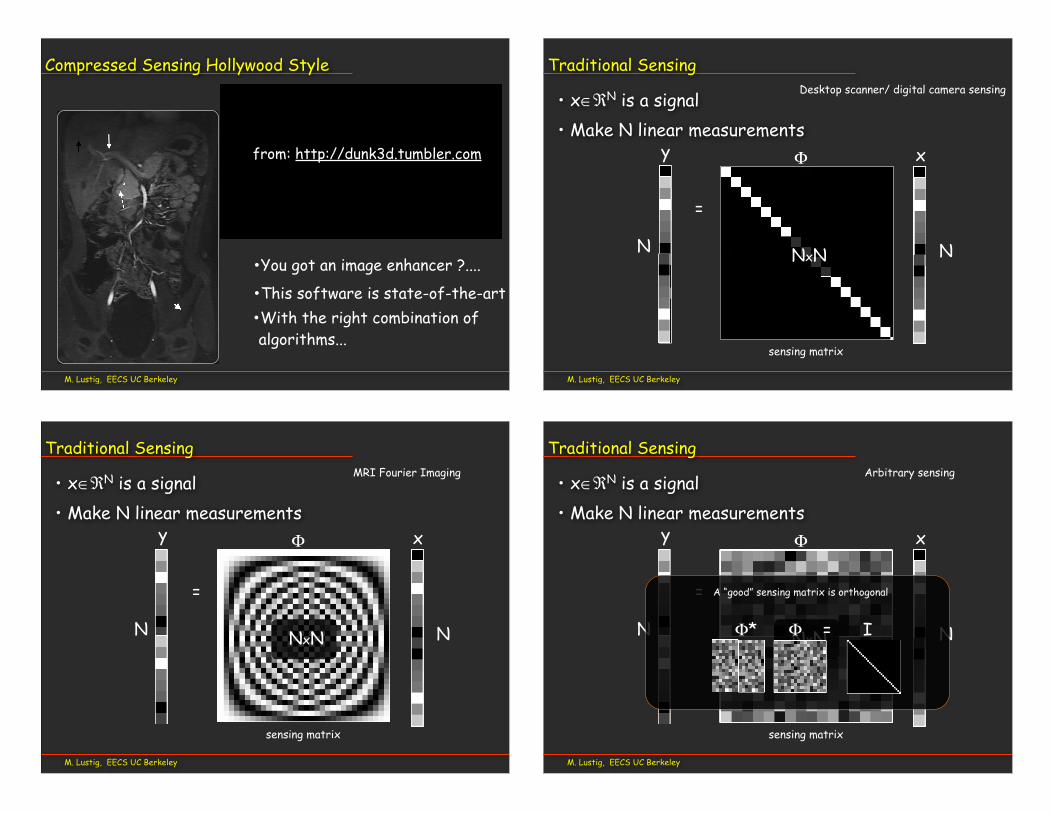
• Accelerated Cine Turbo-Spin-echo R=10
M. Lustig, EECS UC Berkeley
Example: Dynamic CINE
Courtesy, Denis Parker, University of Utah
2 Averages to avoid artifact Dynamic Cine
Mendes et al, MRM 66:1286, 2011
M. Lustig, EECS UC Berkeley
Example: 3D Real-time
• Real-time airway collapseR = 13
Mid-sagittal
Para-sagittal
Axial slicesSuperior
Inferior
Courtesy, YC Kim & K. Nayak, USC
normal breathing load during inspiration
Marked narrowing
M. Lustig, EECS UC Berkeley
A Surprising Experiment
recon
standard
sensing
Compressed
Randomly throw away84% of samples
Transform
Fourier
Candes, Romberg and Tao; 2004M. Lustig, EECS UC Berkeley
Implications…
Randomly throw away66% of samples
• MRI data are obtained in k-space
• Potential for significant scan time reduction
transform
Fourier
recon
standard
sensing
compressed
M. Lustig, EECS UC Berkeley
Compressed Sensing Hollywood Style
from: http://dunk3d.tumbler.com
•This software is state-of-the-art•With the right combination of algorithms...
•You got an image enhancer ?....
• x∈ℜN is a signal • Make N linear measurements
M. Lustig, EECS UC Berkeley
N N
Traditional Sensing
xy
=
Φ
sensing matrix
NxN
Desktop scanner/ digital camera sensing
• x∈ℜN is a signal • Make N linear measurements
M. Lustig, EECS UC Berkeley
N N
Traditional Sensing
xy
=
Φ
sensing matrix
NxN
MRI Fourier Imaging
M. Lustig, EECS UC Berkeley
N N
Traditional Sensing
• x∈ℜN is a signal • Make N linear measurements
xy
=
Φ
sensing matrix
NxN
A “good” sensing matrix is orthogonal
Φ* Φ = I
Arbitrary sensing
M. Lustig, EECS UC Berkeley
sensing matrix
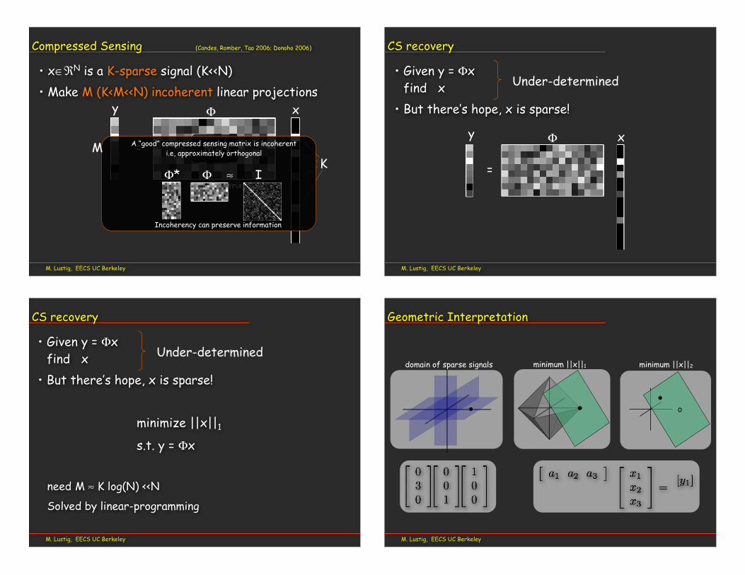
Compressed Sensing (Candes, Romber, Tao 2006; Donoho 2006)
• x∈ℜN is a K-sparse signal (K<<N)• Make M (K<M<<N) incoherent linear projections
x
=
Φ
MxNK
sensing matrix
A “good” compressed sensing matrix is incoherent i.e, approximately orthogonal
Φ* Φ ≈ I
Incoherency can preserve information
M
y
M. Lustig, EECS UC Berkeley
CS recovery
• Given y = Φxfind x
• But there’s hope, x is sparse!
Under-determined
=
Φ xy
M. Lustig, EECS UC Berkeley
CS recovery
• Given y = Φxfind x
• But there’s hope, x is sparse!
minimize ||x||1
s.t. y = Φx
need M ≈ K log(N) <<N
Solved by linear-programming
Under-determinedminimum ||x||1 minimum ||x||2
M. Lustig, EECS UC Berkeley
Geometric Interpretation
domain of sparse signals
M. Lustig, EECS UC Berkeley
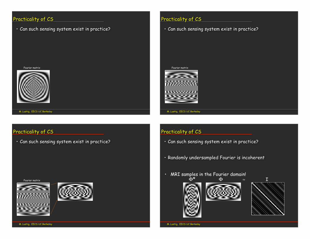
Practicality of CS
• Can such sensing system exist in practice?
Fourier matrix
M. Lustig, EECS UC Berkeley
Practicality of CS
• Can such sensing system exist in practice?
Fourier matrix
M. Lustig, EECS UC Berkeley
Practicality of CS
• Can such sensing system exist in practice?
Fourier matrix
M. Lustig, EECS UC Berkeley
• Can such sensing system exist in practice?
• Randomly undersampled Fourier is incoherent
Φ* Φ ≈ I
Practicality of CS
=
• MRI samples in the Fourier domain!
M. Lustig, EECS UC Berkeley
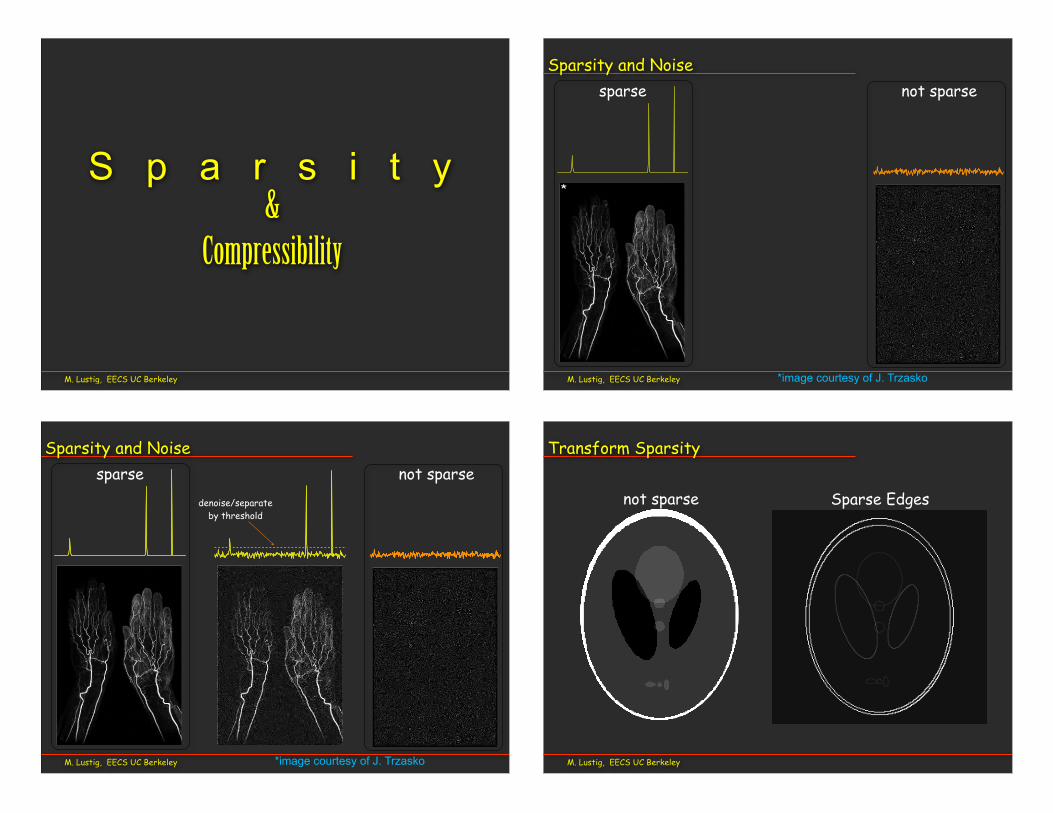
S p a r s i t y &
Compressibility
not sparsesparse
M. Lustig, EECS UC Berkeley
Sparsity and Noise
*image courtesy of J. Trzasko
*
M. Lustig, EECS UC Berkeley
Sparsity and Noise
*image courtesy of J. Trzasko
sparse not sparse
*
denoise/separate by threshold
M. Lustig, EECS UC Berkeley
Transform Sparsity
not sparse Sparse Edges
M. Lustig, EECS UC Berkeley
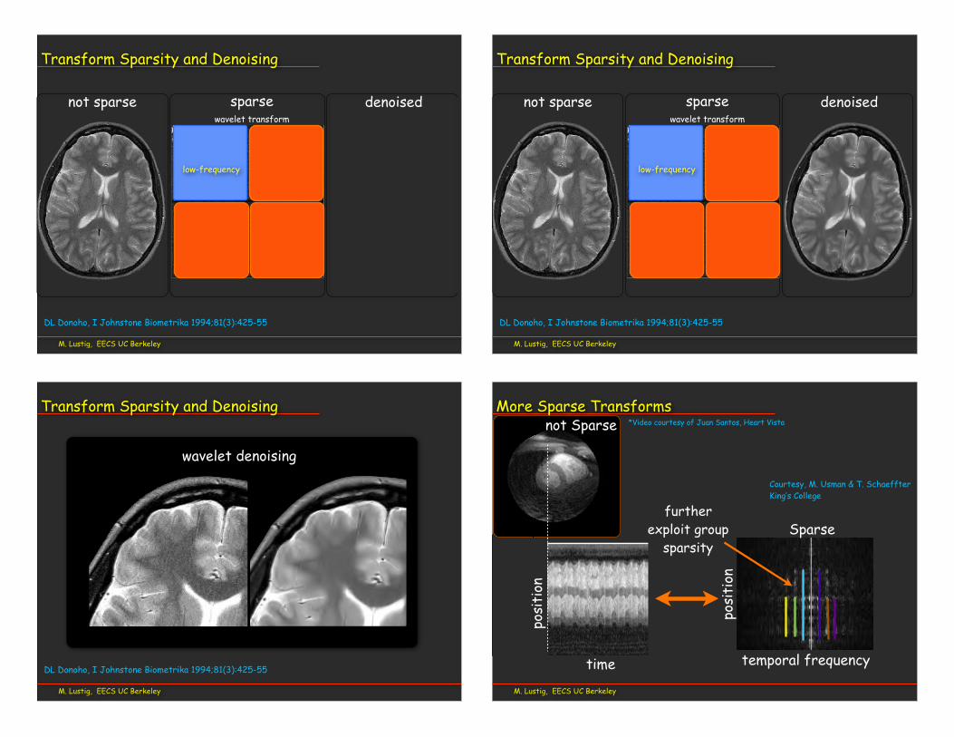
Transform Sparsity and Denoising
sparsenot sparsewavelet transform
low-frequency
high frequency
denoised
DL Donoho, I Johnstone Biometrika 1994;81(3):425-55
M. Lustig, EECS UC Berkeley
Transform Sparsity and Denoising
sparsenot sparsewavelet transform
denoised
low-frequency
high frequency
DL Donoho, I Johnstone Biometrika 1994;81(3):425-55
M. Lustig, EECS UC Berkeley
Transform Sparsity and Denoising
wavelet denoising
DL Donoho, I Johnstone Biometrika 1994;81(3):425-55
M. Lustig, EECS UC Berkeley
More Sparse Transforms
time
posi
tion
posi
tion
temporal frequency
Sparse
not Sparse *Video courtesy of Juan Santos, Heart Vista
Courtesy, M. Usman & T. SchaeffterKing’s College
furtherexploit group
sparsity
M. Lustig, EECS UC Berkeley
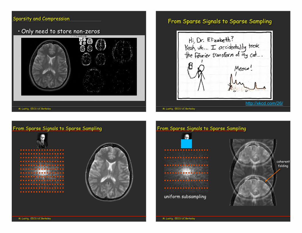
Sparsity and Compression
• Only need to store non-zeros
M. Lustig, EECS UC Berkeley
http://xkcd.com/26/
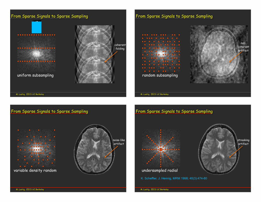
From Sparse Signals to Sparse Sampling
M. Lustig, EECS UC Berkeley
From Sparse Signals to Sparse Sampling
M. Lustig, EECS UC Berkeley
From Sparse Signals to Sparse Sampling
uniform subsampling
coherentfolding
M. Lustig, EECS UC Berkeley
From Sparse Signals to Sparse Sampling
coherentfolding
uniform subsampling
M. Lustig, EECS UC Berkeley
From Sparse Signals to Sparse Sampling
random subsampling
non-coherentartifact
M. Lustig, EECS UC Berkeley
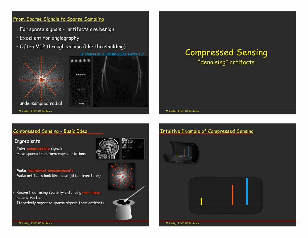
From Sparse Signals to Sparse Sampling
variable density random
noise-likeartifact
M. Lustig, EECS UC Berkeley
From Sparse Signals to Sparse Sampling
K. Scheffler, J. Hennig, MRM 1998; 40(3):474-80
undersampled radial
streakingartifact
M. Lustig, EECS UC Berkeley
From Sparse Signals to Sparse Sampling
D. Peters et. al, MRM 2000; 43:91-101
better resolution than the 4003 400 FT (512 with 1.3 largerFOV). This places a lower limit on the actual resolution ofundersampled PR in this imaging situation.
Human StudiesThis section presents the results from four contrast-enhanced exams, out of the 10 exams conducted using PRwith contrast agent in healthy volunteers and a patient.
ZIPR With Progressively Fewer ProjectionsFigure 7 shows the femoral arteries imaged with ZIPRduring contrast agent infusion, originally collected as a 512(312 acquired) 3 400 projection angle PR image using thefollowing parameters: 40 3 40 3 11.2 cm FOV, 30° tip,TR/TE of 8.0 ms/1.1 ms, 664 kHz BW, 312 3 400 projec-tions3 16 kz3 1 frame acquisition matrix, 5123 5123 16reconstruction matrix, 0.78 3 0.78 3 7.0 mm true voxelsize, 51 s scan time, 0.3 mmol/kg at 0.5 ml/s gadoliniumcontrast agent injection, and torso phased array coil.Images were reconstructed with progressively fewer angles(using (a) 400, (b) 200, (c) 100, and (d) 50 angles) byskipping angles in the full dataset. The changing imagequality is due to the worsening of artifacts and reduction ofSNR at lower numbers of projections. Nevertheless, clini-
FIG. 6. Quantitative resolution comparison between FT and PR inthe resolution phantom for FT acquisitions with 512 phase encodings,400 phase encodings, 128 phase encodings, and PR with 128projections. The magnitude of oscillations for each dot pattern isrecorded. The 128 PR method performs similarly to the 512 FTmethod, and better than the 400 FT method.
a b cFIG. 5. Resolution comparison between FT and PR. a: FT 5123 128 phase encodings. b: PR 5123 128 projections. c: FT 5123 512 phaseencodings. The pixel resolution of the 512 3 512 image is 0.3 3 0.3 mm, and the smallest dots are 0.5 mm wide, spaced 0.5 mm apart. Theundersampled PR image has resolution similar to the 512 3 512 FT image, although it was acquired in one-fourth of the time. The Fourierfrequency-encoding direction is indicated by the arrow.
Undersampled PR for MRA 95
cally significant detail is present, even with 50 projections(an undersampling factor of 16 relative to fully sampledPR).
ZIPR Comparisons Between FT and PR in HumansTo evaluate undersampled PR for contrast-enhanced MRA,3D volumes obtained using the FT and PR imaging meth-ods were compared in a contrast-enhanced scan of thepulmonary vessels. MIP comparisons between FT (512 3128 phase encodings) and PR (512 3 128 projections) arepresented in Fig. 8. The following parameters were used:36 3 36 3 12.8 cm FOV, 30° tip, TR/TE 7.5 ms/1.2 ms,664 kHz BW, 312 3 128 projections or phase encodings 332 kz 3 1 frame acquisition matrix, 512 3 512 3 64reconstruction matrix, 0.70 3 0.70 3 4 mm true voxel sizefor PR, 0.7 3 2.8 3 4 mm true voxel size for FT, 31 s scantime, 18 ml at 1 ml/s gadolinium contrast agent injection,and a torso phased array coil. Minimal undersamplingartifact is visible in the PR images. The comparison clearlyillustrates significant improvement in resolution for PR inthe Fourier phase encoding (horizontal) direction. The FT
MIPs show better SNR and more vessels. The PR imageshave sharper vessels.
Fast Pulmonary ImagingOne use of undersampled PR is for fast moderate-resolution imaging. For example, patients with suspectedpulmonary embolism can only tolerate short breathholds.In Fig. 9 we compare contrast-enhanced FT and PR
pulmonary angiograms both obtained in a 17-sec breath-hold. We compare targeted MIPs of the undersampled PRand FT. The scan parameters for PRwere: 363 363 9.6 cmFOV, 40° tip, TR/TE 5 6.0 ms/1.2 ms, 664 kHz BW, 400(240 acquired) 3 170 projections 3 16 kz, 512 3 512 3 32reconstruction matrix, true voxel size 0.9 3 0.9 3 6 mm,27 mls at 2 ml/s gadolinium contrast agent injection, fatsuppression pulse once per slice loop, and a cardiacphased array coil. For the FT scan (Fig. 9b), all parameterswere the same except 256 xres (160 acquired) and a 128phase encodings resulting in 1.43 2.83 6.0 mm true voxelsize. The comparison shows the much better resolution of
a
c
b
dFIG. 7. ZIPR MIPs of the femoral arteries, all generated from the same data set using progressively fewer number of projections: (a) 400, (b)200, (c) 100, (d) 50. Even with 50 projections (d), clinically significant detail is present. The origin of the profunda femoral artery at the commonfemoral artery is well depicted.
96 Peters et al.
undersampled radial
• For sparse signals - artifacts are benign• Excellent for angiography• Often MIP through volume (like thresholding)
M. Lustig, EECS UC Berkeley
Compressed Sensing “denoising” artifacts
M. Lustig, EECS UC Berkeley
• Take compressible signals Have sparse transform representations
• Make incoherent measurements Make artifacts look like noise (after transform)
• Reconstruct using sparsity-enforcing non-linear reconstructionIteratively separate sparse signals from artifacts
Compressed Sensing - Basic Idea
Ingredients:
M. Lustig, EECS UC Berkeley
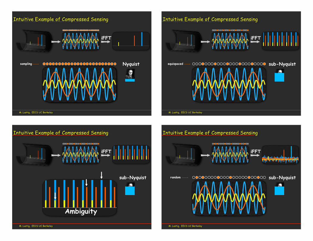
Intuitive Example of Compressed Sensing
M. Lustig, EECS UC Berkeley
Intuitive Example of Compressed Sensing
iFFT
Nyquistsampling
M. Lustig, EECS UC Berkeley
Intuitive Example of Compressed Sensing
iFFT
sub-Nyquistequispaced
M. Lustig, EECS UC Berkeley
Intuitive Example of Compressed Sensing
iFFT
sub-Nyquist
Ambiguity
M. Lustig, EECS UC Berkeley
Intuitive Example of Compressed Sensing
iFFT
sub-Nyquistrandom

M. Lustig, EECS UC Berkeley
Intuitive Example of Compressed Sensing
iFFT
sub-NyquistLooks like
“random noise”
M. Lustig, EECS UC Berkeley
Intuitive Example of Compressed Sensing
iFFT
sub-NyquistBut it’s not
noise!
M. Lustig, EECS UC Berkeley
Intuitive example of CS
iFFT
Recovery
Example inspired by Donoho et. Al, 2007
M. Lustig, EECS UC Berkeley
Question!
• What if the signal is sparse, and we sample it directly?
• Would CS still work?
sub-Nyquistrandom sub-Nyquist

M. Lustig, EECS UC Berkeley
Answer...
• What if the signal is sparse, and we sample it directly?
• Would CS still work?
sub-Nyquistrandom sub-Nyquist
Most likely we will get only zeros!M. Lustig, EECS UC Berkeley
Domains in Compressed Sensing
Signal
SparseDomain
SamplingDomain
Not Sparse!
Sparse! incoherent
M. Lustig, EECS UC Berkeley
Domains in CS MRI
Signal
k-space
Wavelet domain incoherent
Signal domain
M. Lustig, EECS UC Berkeley
Domains in CS MRI
x-f domain incoherent
k-t domainx-t domain
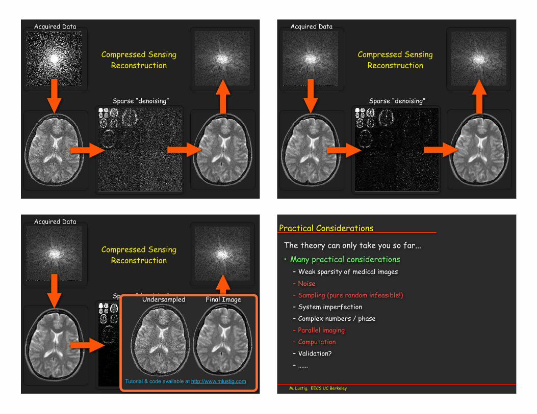
Acquired Data
Sparse “denoising”
Compressed SensingReconstruction
Acquired Data
Sparse “denoising”
Compressed SensingReconstruction
Acquired Data
Sparse “denoising”Undersampled Final Image
Compressed SensingReconstruction
Tutorial & code available at http://www.mlustig.comM. Lustig, EECS UC Berkeley
Practical Considerations
The theory can only take you so far... • Many practical considerations
– Weak sparsity of medical images
– Noise
– Sampling (pure random infeasible!)
– System imperfection
– Complex numbers / phase
– Parallel imaging
– Computation
– Validation?
– ......

• Noise– Noise in the sparse domain counts!– Subsampling reduces SNR– Resulting image noise is not white-Gaussian– Apparent SNR ≠ Sensitivityonly use when SNR is sufficient!
M. Lustig, EECS UC Berkeley
Limitations and Pitfalls
remainingartifact “noise” True noise
M. Lustig, EECS UC Berkeley
Artifacts
Blurred Blocky Good quality
• Artifacts: ( when pushed to limits)
• Usually easy to recognize• Can be subtle
– Washed contrast
– Loss of resolution
– Synthetic/artificial look
– Blocky artifacts
Example courtesy M. Uecker, UCB
M. Lustig, EECS UC Berkeley
Trade-offs
• CS provides new tradeoffs– Loss of low-contrast
features instead of resolution
acce
lera
tion
Low-Resolution Compressed Sensing
M. Lustig, EECS UC Berkeley
Incoherent sampling3D “Full” 3D “Compressed”
M. Lustig, EECS UC Berkeley
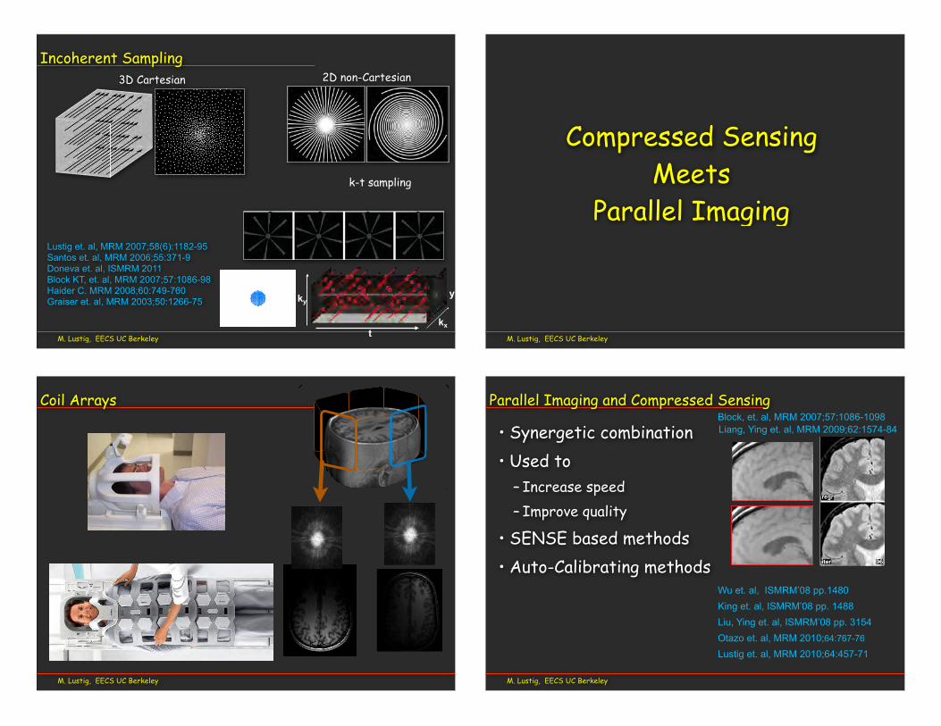
Incoherent Sampling
t
kyy
kx
2D non-Cartesian3D Cartesian
k-t sampling
Lustig et. al, MRM 2007;58(6):1182-95Santos et. al, MRM 2006;55:371-9Doneva et. al, ISMRM 2011Block KT, et. al, MRM 2007;57:1086-98Haider C. MRM 2008;60:749-760Graiser et. al, MRM 2003;50:1266-75
M. Lustig, EECS UC Berkeley
Compressed Sensing Meets
Parallel Imaging
M. Lustig, EECS UC Berkeley
Coil Arrays
M. Lustig, EECS UC Berkeley
Parallel Imaging and Compressed Sensing
• Synergetic combination• Used to
– Increase speed– Improve quality
• SENSE based methods• Auto-Calibrating methods
Block, et. al, MRM 2007;57:1086-1098
Wu et. al, ISMRM’08 pp.1480King et. al, ISMRM’08 pp. 1488Liu, Ying et. al, ISMRM’08 pp. 3154Otazo et. al, MRM 2010;64:767-76
Lustig et. al, MRM 2010;64:457-71
Liang, Ying et. al, MRM 2009;62:1574-84
M. Lustig, EECS UC Berkeley
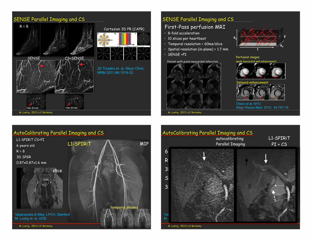
SENSE Parallel Imaging and CS
1030 Trzasko et al.
FIG. 7. Selected images from Example 5: (a–c) are coronal MIPs of early, middle, and late filling stage volumes from a nonview-sharedSENSE + Homodyne reconstruction of the calves of a volunteer, and (d) is an axial cross-section of a middle filling stage volume; (e–g) and(h) are from the corresponding NCCS reconstruction. The location of the axial cross-section is marked by the dotted line in (b) and (f). (i) and(j) are the respective enlargements of an ROI in (b) and (f); (k) and (l) are the respective enlargements of an ROI in (d) and (h).
Another limitation of the proposed reconstruction strat-egy is that both the recovery model and the numericaloptimization routine each possess several parameters thatmust be reasonably assigned to achieve high quality results.For example, assigning too small a value to the regulariza-tion parameter, α, can allow noise amplification during thereconstruction, whereas assigning too large a value to α canresult in over-sparsification and thus over-smoothing of theimage, and a corresponding loss of features. However, it isnoted that once an effective setting is found for a particu-lar image scenario, it can be reused (e.g., all neurovascularstudies are run under the same settings).
Although beyond the scope of this manuscript, it isexpected that the improved vessel-to-background con-spicuity (i.e., contrast) and homogeneity of vessels, enhanc-ing structures, and background tissue resulting from theNCCS reconstruction strategy for CAPR CE-MRA imageseries will lead to improved diagnosis, with better sen-sitivity for detection of abnormalities, and fewer falsepositive/negative interpretations. Nonetheless, a formalradiological comparison of these two reconstruction strate-gies is still needed and will be the subject of a separate,future work.
APPENDIX: FINITE SPATIAL DIFFERENCECOMPUTATION
The adopted finite difference spatial model assumes thatany finite spatial difference centered inside Ω but for whichthe neighbor of interest is outside Ω will be zero. Morespecifically, ∀s ∈ Ω and any n,
[Dnu](s) =
u(s) − u(s + n), if (s + n) ∈ Ω
0, else .
Note that this operator can be abstracted as Dn = I −Sn−Cn,where I is the identity operator, Sn is a non-wrapped shiftoperator (towards neighbor n) with zero-filling, and Cn isan operator that copies nonshifted boundary elements. Letn = ∆x , ∆y , ∆z and s = x, y , z, where x ∈ [0, Nx ), y ∈[0, Ny ), and z ∈ [0, Nz). Assuming the notation u(s + n) =u(x + ∆x , y + ∆y , z + ∆z), the component operators of Dncan then be defined as
[Snu](s) =
u(s + n), if (x ∈ Υx ) ∧ (y ∈ Υy ) ∧ (z ∈ Υz)0, else
[20]
JD Trzasko et. al, Mayo ClinicMRM 2011;66:1019-32
R = 8
SENSE CS+SENSE
raw slices raw slices
Cartesian 3D PR (CAPR)1020 Trzasko et al.
FIG. 1. An example W = 4 CAPR acquisition sequence (Ny = Nz = 256). During this acquisition, the phase-encoded plane of k-space(ky-kz) is partitioned into a distinct low-pass region, shown in orange, and a high-pass region (a). The high-pass annulus is itself furtherpartitioned azimuthally into W subsets of “vanes,” shown here in blue, green, yellow, and red, which are placed asymmetrically aboutthe origin. Although Cartesian, the CAPR sampling operator, by construction, tends to exhibit properties similar to non-Cartesian radialtrajectories (within the phase-encoded plane). The sampling order or schedule is shown in (b). During each temporal update, uniformly-spaced samples (here, spaced 2 × 2 apart) from within the low-pass region and a single high-pass vane set are acquired. This same set ofk-space indices is reinvestigated after W temporal updates. The set of all k-space indices investigated at any point during the entire exam isshown in (c) and is simply the union of the sample sets shown in (b). Note that, for this example, only about 20% of k-space is investigatedduring the exam, a property that facilitates practical formation of the reference signal needed for background subtraction.
THEORY
A Forward Model for Parallel MRI
Suppose we are interested in forming a discrete image esti-mate of some anatomy of interest using three-dimensionalCartesian (3DFT) parallel magnetic resonance imaging.Denoting f as the discrete image of interest, a commonly-assumed forward model for this acquisition process is
g1g2...
gC
=
ΦFΓ1ΦFΓ2
...ΦFΓC
f + n, [1]
where gc is the signal observed by the cth coil sensor, Γcis the element-wise (i.e., diagonal) spatial sensitivity func-tion for the cth coil sensor, F is the discrete 3D Fouriertransform (3DFT) operator, and Φ is a binary operator thatidentifies the subset of k-space measured during the imag-ing experiment. The vector n represents system noise and ishereafter assumed to be a complex additive white Gaussianprocess (13).
Time-Varying Signals and CAPR
In CE-MRA, the signal of interest is inherently tran-sient and thus routinely probed at multiple different timepoints to characterize patient hemodynamics in addi-tion to vascular morphology. Given the direct relationshipbetween the number of k-space indices measured duringan MRI exam and the duration of the exam, spatiotemporalundersampling is often employed to accelerate dynamic
MRI exams such as CE-MRA. Reconstruction techniquessuch as view-sharing (25), HYPR-type processing (8,26),and constraint or regularization methods (9,23,27–33) thatrely on a priori assumptions about spatial and/or temporalimage structure may be employed to avoid generation ofimages with significant artifacts.
Assuming that both the signal of interest and the sam-pling process may be temporally variant in dynamic MRI,(1) can be generalized to
g1(t)g2(t)
...gC (t)
=
Φ(t)FΓ1Φ(t)FΓ2
...Φ(t)FΓC
f (t) + n(t), [2]
where t ≥ 0 is an integer corresponding to the frame num-ber. During a CAPR acquisition, k-space is partitioned intotwo distinct regions: (1) a circularly-symmetric low-passregion that is sampled during each temporal update; (2)a high-pass region of which a different subset is sampledduring each temporal update. Thus, the effective samplingoperator for CAPR can be described as
Φ(t) =[
ΦLOΦHI(t)
]. [3]
The dynamic high-pass sampling operator ΦHI(t) is alsostrictly W -periodic and so, ∀t ≥ 0, ΦHI(t) = ΦHI(t+W ), and∀τ ∈ (0, W ), Trace(Φ*
HI(t+τ)ΦHI(t)) = 0. A pictorial exampleof a CAPR acquisition sequence is given in Fig. 1. For a moredetailed description of the CAPR acquisition protocol, thereader is referred to (11).
M. Lustig, EECS UC Berkeley
SENSE Parallel Imaging and CS
• 8-fold acceleration• 10 slices per heartbeat• Temporal resolution = 60ms/slice• Spatial resolution (in-plane) = 1.7 mm• SENSE +PI
Perfusion images(peak myocardial wall enhancement)
Delayed-enhancement
Otazo et al. NYUMagn Reson Med. 2010; 64:767-76
Patient with acute myocardial infarction
First-Pass perfusion MRI
t
kyy
kx
M. Lustig, EECS UC Berkeley
AutoCalibrating Parallel Imaging and CSL1-SPIRiT CS+PI6 years oldR = 83D SPGR0.87x0.87x1.6 mm
Vasanawala & Alley, LPCH, StanfordM. Lustig et. al, UCB
MIP
slice
L1-SPIRiT
temporal phases
M. Lustig, EECS UC Berkeley
AutoCalibrating Parallel Imaging and CS
6 years old maleR = 83D SPGRSub-mm32 channels
L1-SPIRiTPI + CS
autocalibratingParallel Imaging
Vasanawala & Alley, LPCH, StanfordM. Lustig et. al, UCB

M. Lustig, EECS UC Berkeley
Compressed Sensing in the Clinic
• Target: Robust, sedation-free pediatric body MRI
• Leverage:dedicated 32ch coilCompressed SensingMotion CorrectionParallel Computing
• ~6 clinical scan / day at LPCHsince 2010
dedicated 32Ch coil
GPU’s & multi-core CPU
Berkeley Stanford GE
M. Lustig, EECS UC Berkeley
Reconstruction speed
• Iterative reconstruction computationally intensive• Large data-sets are better for CS • Currently top hurdle in penetration to clinic• Current Solutions:
– Algorithmic – Parallel Computation
D. Kim, J. Trzasko, A. Manduca et. al “High Performance 3D CS MRI Reconstruction Using Many-Core Architectures, IJBI doi:10.1155/2011/473123Intel and Mayo Clinic
1-3min for 3D datasets
M. Murphy, M. Lustig et. al, “Fast L1-SPIRiT CS PI MRI:Parallel Implementation and Clinically Feasible Scan-Time” IEEE-TMI 2012; early viewUC Berkeley, Stanford University
M. Lustig, EECS UC Berkeley
Emerging Techniquesand Applications
M. Lustig, EECS UC Berkeley
Multi-Contrast Reconstruction• An exam consists of multiple scans• Mutual information between exams• Jointly reconstruct all exams
joint reconseparate recon*B. Bilgic et. al, MIT MRM 2011;66:1601-15,
err.
x10
R=2.
4
T1w
T2w
+F. Huang, ISMRM ’12 pp2539 Philips
R=5
err.
x5
M. Lustig, EECS UC Berkeley
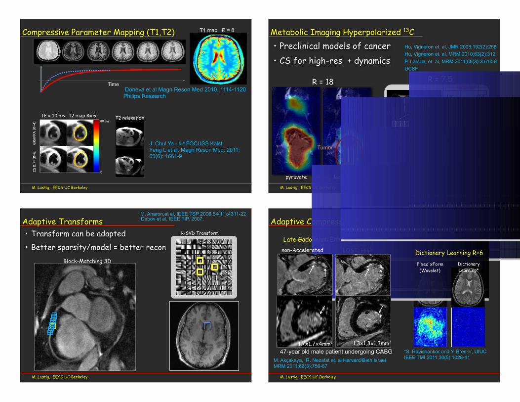
Compressive Parameter Mapping (T1,T2)CS#&#PI#(R=
6)GR
APPA
#(R=4)
TE#=#10#ms T2#map#R=#6
0
80#ms
J. Chul Ye - k-t FOCUSS KaistFeng L et al. Magn Reson Med. 2011; 65(6): 1661-9
Doneva et al Magn Reson Med 2010, 1114-1120Philips Research
Time
T1 map R = 8
T2#relaxa=on
• Preclinical models of cancer• CS for high-res + dynamics
M. Lustig, EECS UC Berkeley
Metabolic Imaging Hyperpolarized 13C
R = 7.5
Hu, Vigneron et. al, JMR 2008;192(2):258Hu, Vigneron et. al, MRM 2010;63(2):312P. Larson, et. al, MRM 2011;65(3):3:610-9UCSF
Regular
Compressedsensing
R = 18
Tumor
pyruvate lactate
• Transform can be adapted• Better sparsity/model = better recon
M. Lustig, EECS UC Berkeley
k-SVD Transform
S. Ravishankar and Y. Br
Adaptive Transforms Dabov et al, IEEE TIP, 2007.M. Aharon,et al, IEEE TSP 2006;54(11):4311-22
Block-Matching 3D
M. Lustig, EECS UC Berkeley
Adaptive Compressed Sensing
LOST: High-res
Late Gadolinium Enhancement R=3
2D Random Sampling - 6 fold undersampling
0
0.05
0.1
0.15
0.2
0.25
0.3
LDP reconstruction (22 dB) LDP error magnitude
0
0.05
0.1
0.15
0.2
0.25
0.3
DLMRI reconstruction (32 dB) DLMRI error magnitude
S. Ravishankar and Y. Bresler DLMRI
2D Random Sampling - 6 fold undersampling
0
0.05
0.1
0.15
0.2
0.25
0.3
LDP reconstruction (22 dB) LDP error magnitude
0
0.05
0.1
0.15
0.2
0.25
0.3
DLMRI reconstruction (32 dB) DLMRI error magnitude
S. Ravishankar and Y. Bresler DLMRI
2D Random Sampling - 6 fold undersampling
0
0.05
0.1
0.15
0.2
0.25
0.3
LDP reconstruction (22 dB) LDP error magnitude
0
0.05
0.1
0.15
0.2
0.25
0.3
DLMRI reconstruction (32 dB) DLMRI error magnitude
S. Ravishankar and Y. Bresler DLMRI
2D Random Sampling - 6 fold undersampling
0
0.05
0.1
0.15
0.2
0.25
0.3
LDP reconstruction (22 dB) LDP error magnitude
0
0.05
0.1
0.15
0.2
0.25
0.3
DLMRI reconstruction (32 dB) DLMRI error magnitude
S. Ravishankar and Y. Bresler DLMRI
Fixed xForm (Wavelet)
DictionaryLearning*
*S. Ravishankar and Y. Bresler, UIUCIEEE TMI 2011;30(5):1028-41
non-Accelerated Dictionary Learning R=6
M. Akçakaya, R. Nezafat et. al Harvard/Beth IsraelMRM 2011;66(3):756-67
1.3x1.3x1.3mm31.7x1.7x4mm3
47-year old male patient undergoing CABG
M. Lustig, EECS UC Berkeley
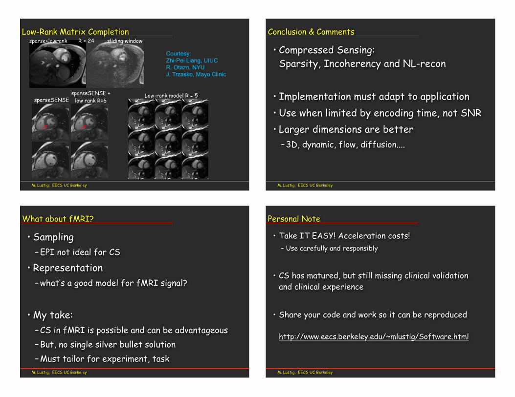
Low-Rank Matrix CompletionR = 24
sparseSENSE + low rank R=6
sparse+lowrank sliding window
sparseSENSE Low-rank model R = 5
Courtesy:Zhi-Pei Liang, UIUCR. Otazo, NYUJ. Trzasko, Mayo Clinic
M. Lustig, EECS UC Berkeley
Conclusion & Comments
• Compressed Sensing: Sparsity, Incoherency and NL-recon
• Implementation must adapt to application• Use when limited by encoding time, not SNR• Larger dimensions are better
– 3D, dynamic, flow, diffusion....
M. Lustig, EECS UC Berkeley
What about fMRI?
• Sampling– EPI not ideal for CS
• Representation– what’s a good model for fMRI signal?
• My take:– CS in fMRI is possible and can be advantageous– But, no single silver bullet solution– Must tailor for experiment, task
M. Lustig, EECS UC Berkeley
Personal Note
• Take IT EASY! Acceleration costs!– Use carefully and responsibly
• CS has matured, but still missing clinical validation and clinical experience
• Share your code and work so it can be reproduced
http://www.eecs.berkeley.edu/~mlustig/Software.html

M. Lustig, EECS UC Berkeley
AcknowledgmentsSLIDES:
• Brian Hargreaves, Stanford
• Pauline Worters, Stanford
• Shreyas Vasanawala, Stanford
• Yoram Bresler, UIUC
• Zhi-Pei Liang, UIUC
• Denis Parker, Uni. of Utah
• Leslie Ying, Buffalo
• Reza Nezafat , BIDMC
• M. Akçakaya
• Feng Huang, Phillips
• Mariya Doneva, Phillips
• Anita Flynn, Berkeley
• Tobias Schaeffter, King’s College
• Muhammad Usman, king’s College
• Daniel Vigneron, Peder Larson, UCSF
• Jonh Chul-Ye, Kaist
• Berkin Bilgic, Elfar Adalsteinsson, MIT
• Maxim Zaitsev, Freiburg
• Martin Uecker, Max Planck & Berkeley
• Luca Marinelli, GE global research
• Ricardo Otazo, NYU
• Chuck Mistretta, Yijing Wu, UW
• Julia Velikina, Alexey Samsonov, UWNIH R01-EB009690, RR09794-15
GE Healthcare
Morgridge Foundation
American Heart Association
UC Discovery
“Everything to do with compression is very contentious in medical imaging. Every time you throw bits away somebody gets very nervous about it. The fortunate thing about ....[compressed sensing]... is that you don’t collect them in the first place, and that’s a much better situation!”
John Pauly 2007
Thank Youתודה רבה
http://www.eecs.berkeley.edu/~mlustig