Spacecraft Relative Attitude Formation Tracking on SO(3)Based on Line-of-Sight Measurements

by Tse-Huai Wu

B.S. in Power Mechanical Engineering, May 2008, National Tsing Hua University

A Thesis submitted to

The Faculty ofThe School of Engineering and Applied Science

of The George Washington Universityin partial fulfillment of the requirements

for the degree of Master of Science

January 31, 2013

Thesis directed by

Taeyoung LeeAssistant Professor of Engineering and Applied Science

c© Copyright 2013 by Tse-Huai WuAll Rights Reserved

ii

Dedication

I dedicate this thesis to Mom and Dad. I am blessed to be their son.

iii

Abstract of Thesis

Spacecraft Relative Attitude Formation Tracking On SO(3) Based on Line-of-SightMeasurements

This thesis investigates the use of line-of-sight (LOS) measurements for the control of

relative attitude formation among multiple spacecraft. It is based on the fact that two

pointing directions, referring to LOS measurements, from the spacecraft to distinct

objects can determine the absolute attitude of spacecraft. With the same approach,

LOS measurements from cost-effective vision-based sensors can be applied to obtain

the relative attitude among spacecraft. In the proposed approach, high accuracy

of attitude control and simpler control scheme can be constructed by designing the

control law in terms of LOS measurements. In addition, the relative attitude controller

provides almost global exponential stability on the nonlinear configuration manifold

of relative attitude. The described properties are illustrated by numerical examples.

In conventional approaches, the absolute attitude is measured locally by using

an inertial measurement unit, and they are compared to determine relative attitude,

thereby causing the accumulation of measurement errors and complex controller struc-

tures.

iv

Table of Contents

Dedications iii

Abstract of Thesis iv

List of Figures viii

1 Introduction 1

1.1 Motivation . . . . . . . . . . . . . . . . . . . . . . . . . . . . . . . . . 1

1.2 Literature Review . . . . . . . . . . . . . . . . . . . . . . . . . . . . . 3

1.3 Thesis Outline . . . . . . . . . . . . . . . . . . . . . . . . . . . . . . . 5

1.4 Contributions . . . . . . . . . . . . . . . . . . . . . . . . . . . . . . . 6

2 Tracking control of A Spherical Pendulum on the Two-Sphere 9

2.1 Equation of Motion . . . . . . . . . . . . . . . . . . . . . . . . . . . . 9

2.2 PD Tracking Control of a Spherical Pendulum on Two-Sphere . . . . 12

2.2.1 Error Dynamics . . . . . . . . . . . . . . . . . . . . . . . . . . 12

2.2.2 Control System Design . . . . . . . . . . . . . . . . . . . . . . 17

2.3 PID Tracking Control of a Spherical Pendulum on Two-Sphere . . . . 21

2.4 Numerical Example . . . . . . . . . . . . . . . . . . . . . . . . . . . . 23

3 Vision-based Spacecraft Attitude Control on SO(3) 28

3.1 Problem Formulation . . . . . . . . . . . . . . . . . . . . . . . . . . . 28

3.1.1 Attitude Dynamics on SO(3) . . . . . . . . . . . . . . . . . . . 28

v

3.1.2 Vision-Based Attitude Control Problem . . . . . . . . . . . . . 30

3.2 Almost Global Exponential Tracking Control on SO(3) . . . . . . . . 32

3.2.1 Error Variables . . . . . . . . . . . . . . . . . . . . . . . . . . 33

3.2.2 Control System Design . . . . . . . . . . . . . . . . . . . . . . 41

3.3 Numerical Example . . . . . . . . . . . . . . . . . . . . . . . . . . . . 48

4 Spacecraft Relative Attitude Formation Tracking on SO(3) Based

on Line-Of-Sight Measurements 49

4.1 Problem Formulation . . . . . . . . . . . . . . . . . . . . . . . . . . . 49

4.1.1 Spacecraft Attitude Formation Configuration . . . . . . . . . . 50

4.1.2 Spacecraft Attitude Dynamics . . . . . . . . . . . . . . . . . . 54

4.1.3 Kinematics of Relative Attitudes and Line-Of-Sight . . . . . . 55

4.2 Relative Attitude Tracking Between Two Spacecrafts . . . . . . . . . 55

4.2.1 Kinematics of Relative Attitude . . . . . . . . . . . . . . . . . 56

4.2.2 Relative Attitude Tracking . . . . . . . . . . . . . . . . . . . . 66

4.3 Relative Attitude Formation Tracking . . . . . . . . . . . . . . . . . . 72

4.3.1 Relative Attitude Tracking Between Three Spacecrafts . . . . 73

4.3.2 Relative Attitude Formation Tracking Between n Spacecrafts . 78

4.4 Numerical Example . . . . . . . . . . . . . . . . . . . . . . . . . . . . 83

5 Conclusions 85

5.1 Concluding Remarks . . . . . . . . . . . . . . . . . . . . . . . . . . . 85

5.2 Future Work . . . . . . . . . . . . . . . . . . . . . . . . . . . . . . . . 86

Bibliography 88

A Hat Map Identities 93

B The Spectral Theorem 95

vi

C MATLAB Codes 96

vii

List of Figures

Figure2.1 Spherical pendulum . . . . . . . . . . . . . . . . . . . . . . . . . . 10

Figure2.2 Numerical results for spherical pendulum under PD controller with-

out perturbation . . . . . . . . . . . . . . . . . . . . . . . . . . . . . . . 25

Figure2.3 Numerical results for spherical pendulum under PD controller with

fixed perturbation . . . . . . . . . . . . . . . . . . . . . . . . . . . . . . . 26

Figure2.4 Numerical results for spherical pendulum under PID controller . . 27

Figure3.1 Single spacecraft attitude control with LOS measurements . . . . . 29

Figure3.2 Numerical results for single spacecraft attitude control . . . . . . . 48

Figure4.1 Formation of four spacecrafts . . . . . . . . . . . . . . . . . . . . . 53

Figure4.2 Relative attitude formation tracking for 7 spacecrafts . . . . . . . . 82

Figure4.3 Numerical results for seven spacecrafts in formation . . . . . . . . 84

viii

Chapter 1 Introduction

This thesis investigates the use of Line-of-Sight (LOS) measurements for relative

attitude formation between multiple spacecraft. Relative attitude is important in the

multiple spacecraft formation since a constellation of spacecraft should have accurate

relative motion to meet the goal of mission. Based on the approach of geometric

control, the controller in this thesis exhibits exponential stability of the desired time-

varying tracking command with a daisy-chaining structure of multiple spacecraft.

1.1 Motivation

Multiple spacecraft in mission Satellites technology has been widely applied for

communication, navigation, outer space investigation, scientific research or military

purposes. Multiple satellites flying as a group, working together to carry out assigned

tasks, define formation. For instance, in the mission of the Space Technology 5 (ST-

5), three micro-satellites successfully launched in 2006 to explore the magnetic field

of Earth. The Cluster mission of European Space Agency (ESA) with the extend

project Cluster II, cooperated with National Aeronautics and Space Administration

(NASA), has four spacecraft to collect data.

Precise control of relative configuration between spacecraft is critical for manu

cooperative missions [1]. For example, the Space Technology 3 (ST-3) mission is

a space-based interferometer consists of two spacecraft [2]. The interferometer is

an array of telescopes acting jointly to probe structure by means of interferometry.

If telescopes are carried by spacecraft operating in the outer space, various celestial

1

objects can be observed as the spacecraft translate, and high resolution images can be

captured compare to the stationary interferometer on Earth affected by atmospheric

distortion. Also, multiple telescopes can capture the target from different angles or

at different times. Another example is the famous Darwin mission, directed by ESA

and NASA, which is a constellation of four to five spacecraft searching for Earth-like

planets. The images provided by each telescope are combined together such that

Darwin would work as a single large telescope. To do so, the accuracy of relative

position and attitude among spacecraft is critical. The telescopes and the hub must

have stayed in formation with millimeter precision for Darwin to work [3].

Formation Control The spacecraft formation control can be categorized to control

of relative position and relative attitude. Carrier-phase Differential GPS has been

successfully applied to relative position control and estimation [4], [5]. It has been

shown that high precision of GPS technology is effective for relative position control.

As for attitude control, combination of different inertial measurement unit (IMU),

such as accelerometer, gyroscope, or magnetometer, is commonly applied to measure

orientation of spacecraft [6]. There is also a hybrid system using camera and IMU

jointly to perform rotation control [7]. Most of the relative attitude control sys-

tems are based on a common framework: the absolute attitude of the spacecraft,

with respect to an inertial frame, is measured independently by using local inertial

measurement units and then it is transformed to other vehicle to determine relative

attitude. In other words, relative attitude is acquired by comparing the absolute

attitude of each spacecraft.

Measurement errors are accumulated due to this indirect process, and the accuracy

of attitude formation is impaired. When there are more spacecraft in the constellation,

the accumulated error becomes larger. This error problem is not insuperable, but this

approach requires high quality IMU sensors and sophisticated controllers that increase

2

the development cost substantially.

Vision-Based System In recent years, vision-based systems have been applied for

the navigation of autonomous vehicles where optical sensors are used to extract visual

features to locate a vehicle [8], [9]. Specifically, it has been shown that line-of-sight

observations can be applied for relative attitude determination [10]. Optical sensors

are cost-effective with high accuracies, and they have less noises compared with other

inertial sensors. Also, they yield a long-term stability and it requires no frequent

corrections in contrast to gyros.

Global and Unique Representation Typically, attitude control is studied by

using Euler angles or quaternions [11], [12], [13], which are referred to as attitude

parameterizations. None of these parameterizations can successfully represent atti-

tude uniquely and globally. For instance, Euler angles have singularities, therefore,

it is not possible to globally define the control law by using Euler angles. Quaternion

representation does not the have the issue of singularity but there exists ambiguity

since it is not unique in representing attitude. Hence, this thesis proposes to construct

the control system in terms of rotation matrix to control the attitude globally and

uniquely [14].

In summary, the goal of this thesis is to control attitude formation by using line-

of-sight measurements to accomplish high level of performance and cost-effectiveness.

It has desirable feature of accurate relative attitude determination, simple control

structures, low-cost hardware requirement and robust stability.

1.2 Literature Review

Control of the direction of line-of-sight is similar to control the direction of a spherical

pendulum since they evolve in the same configuration space. A spherical pendulum

is a weight bob suspend from a pivot that allows to swing freely in 3-dimensional

3

space. As there is no rotation along the axis direction of the link of the pendulum,

it has 2 rotational degrees of freedom. The direction from pivot to bob is analogous

to the direction of line-of-sight measurements. The nonlinear dynamics of spherical

pendulum has been studied in [15], [16], [17] by using local coordinate. In addition,

Lagrangian mechanical systems on two-spheres has been studied in [18]. If the limi-

tation of axial rotation is removed, the pendulum has 3 rotational degrees of freedom,

which is called 3D pendulum. There is also research about 3D rigid pendulum with

almost global asymptotic stabilization [19], [20].

Attitude control systems are developed in terms of Euler angles [21] or quaternions

[12], [22], [23]. Quaternions do not have singularities like Euler angle. Therefore it

may achieve global attitude tracking properties [24]. However, there is ambiguity in

representing attitude [14]. A phenomenon called “unwinding”, where the close-loop

control input unnecessarily rotates the spacecraft through a large angle even if the

initial attitude error is small, may happen if we do not deal with this ambiguity care-

fully [25]. Nevertheless, there are interesting contributions among these publications.

There is a attitude controller designed for micro-satellite [21]. In [22], a controller

without angular velocity is presented. In [23], control input in saturation is addressed.

Recently, attitude control on special orthogonal group SO(3), the set of three

by three orthogonal matrices with determinant equal to one, has been studied [14],

[26], [27], [28], [29]. The most important feature of this representation is that it the

attitude is determined globally and uniquely.

The coordinated control of multiple spacecraft in formation has been studied ex-

tensively [30], [31]. Notable contributions on relative attitude can be categorized as

leader-follower strategy [32], [13], behavior-based control [33], [34], and virtual struc-

tures [35], [36]. In the leader-follower scheme, one spacecraft on the reference orbit

is assigned to be leader, other spacecraft are followers tracking the relative motion

with respect to the leader. The behavior-based control defines the “behavior” for the

4

spacecraft as the purpose of tasks such as formation keeping or collision avoidance.

Additionally, virtual structure control considers every spacecraft as an element of a

larger, single entity. Some of research even combine two schemes in formation control

[37]. A common drawback of strategy mentioned above, is absolute attitude of each

vehicle must be observed before computing the relative attitude and the measurement

error in each inertial measurement unit is accumulated during this process.

Vision-based sensors combined with image processing are applied in controlling

end-effectors of robot manipulators to reduce positioning error and reduce the overall

cost [38]. Recently, vision-based control systems have been widely applied for nav-

igation of autonomous vehicles, flying or underwater [8], [39]. For instance, in [9],

vision-based control are applied to stabilize a quadrotor. Moreover, the LOS obser-

vations are used for relative attitude determination of multiple vehicles [40], [41].

1.3 Thesis Outline

This thesis is concerned with development of relative attitude control system with

vision based sensors. This is motivated by the fact that control of pointing direction

of line-of-sight measurements on SO(3) is analogous to control the direction of a

spherical pendulum on S2. We start from control a spherical pendulum in the first

step which is the subject of Chapter 2.

In chapter 3, we use vision-based method in the application of attitude control of

single spacecraft. The basic properties and assumptions of vision-based control are

described. The nonlinear structure of SO(3) are explicitly considered in the control

system design, and proof of almost global exponential stability is proposed. These

are extended to the relative attitude control between multiple spacecraft in the next

chapter.

In Chapter 4, the structure of multiple spacecraft is outlined, and work of previous

chapters are combined for relative attitude between multiple spacecraft. We first show

5

the relative attitude control between two spacecraft and then in three spacecraft. By

observing the differences of these two solid examples, we generalized the controller to

multiple spacecraft in the final stage and use the case of 7 spacecraft as an numerical

example.

Each chapter comes with numerical simulations in the final section to demonstrate

the properties of the controlled system.

1.4 Contributions

Vision-based Formation Control The presented control system uses line-of-sight

measurements to control the relative attitude. In other words, the control inputs are

expressed in terms of the direction measurements. Thus, we directly control the rela-

tive attitude without the need for estimating the absolute attitude of each spacecraft.

This scheme is not only simpler than using the traditional inertia measurement units,

but also provides a higher accuracy. Without comparing absolute attitude between

each spacecraft, the issue of accumulated error does not exist in the vision-based

control system which leads to higher accuracy.

In particular, vision-based sensors normally require complex image processing to

extract the information and this causes high computational load. However, we only

need the direction from optical sensors to determine the formation and it requires

relatively low computational cost. Compare to gyroscopes, vision-based sensors do

not need calibration as there is no drift or errors.

Resource sharing and Cost effectiveness As each spacecraft should be equipped

with high accuracy sensors, the total development cost of multiple spacecraft may

become extremely high. Several projects, such as TechSat 21 constellation of three

spacecraft, directed by U.S. Air Force Research Laboratory (AFRL), were canceled

due to cost over budget. From the aspect of allowance, vision-based sensors are

6

relatively inexpensive compare to other hardware systems. Therefore, it reduces

the development cost significantly, especially in large number of spacecraft cluster.

Additionally, as each spacecraft is equipped with onboard visual sensors, we do not

need all of the measurements between them to estimate the corresponding relative

attitude, hence the system can still function well even if some of the sensors break

down.

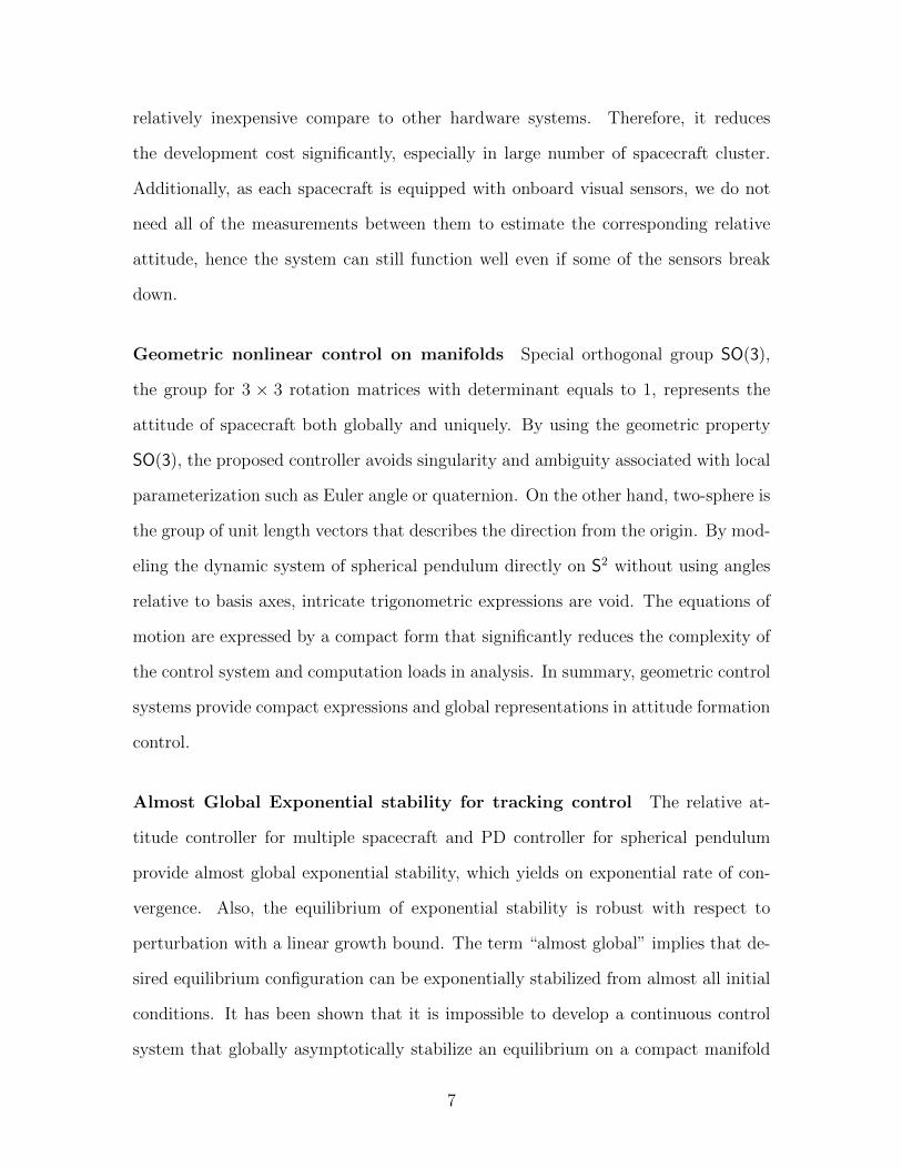
Geometric nonlinear control on manifolds Special orthogonal group SO(3),

the group for 3 × 3 rotation matrices with determinant equals to 1, represents the

attitude of spacecraft both globally and uniquely. By using the geometric property

SO(3), the proposed controller avoids singularity and ambiguity associated with local

parameterization such as Euler angle or quaternion. On the other hand, two-sphere is

the group of unit length vectors that describes the direction from the origin. By mod-

eling the dynamic system of spherical pendulum directly on S2 without using angles

relative to basis axes, intricate trigonometric expressions are void. The equations of

motion are expressed by a compact form that significantly reduces the complexity of

the control system and computation loads in analysis. In summary, geometric control

systems provide compact expressions and global representations in attitude formation

control.

Almost Global Exponential stability for tracking control The relative at-

titude controller for multiple spacecraft and PD controller for spherical pendulum

provide almost global exponential stability, which yields on exponential rate of con-

vergence. Also, the equilibrium of exponential stability is robust with respect to

perturbation with a linear growth bound. The term “almost global” implies that de-

sired equilibrium configuration can be exponentially stabilized from almost all initial

conditions. It has been shown that it is impossible to develop a continuous control

system that globally asymptotically stabilize an equilibrium on a compact manifold

7

such as the two sphere S2 or the special orthogonal group SO(3) due to their topo-

logical properties [42]. The almost global exponential stability is the best result for

continuous control system.

8

Chapter 2 Tracking control of A Spherical Pendulum on

the Two-Sphere

In this chapter, we analyze the dynamics of a spherical pendulum and we present a

nonlinear control system for the time-varying tracking control problem. Pendulum

model without linearization is a good source to accommodate the effect and char-

acteristics of nonlinear dynamics. The control system is directly constructed on the

two-sphere, which is a nonlinear manifold of the spherical pendulum.

The proportional-integral-derivative (PID) controller is the most commonly ap-

plied controller, however, the typical PID controllers are constructed on linear sys-

tems, and a PID controller on the two-sphere has not been studied.

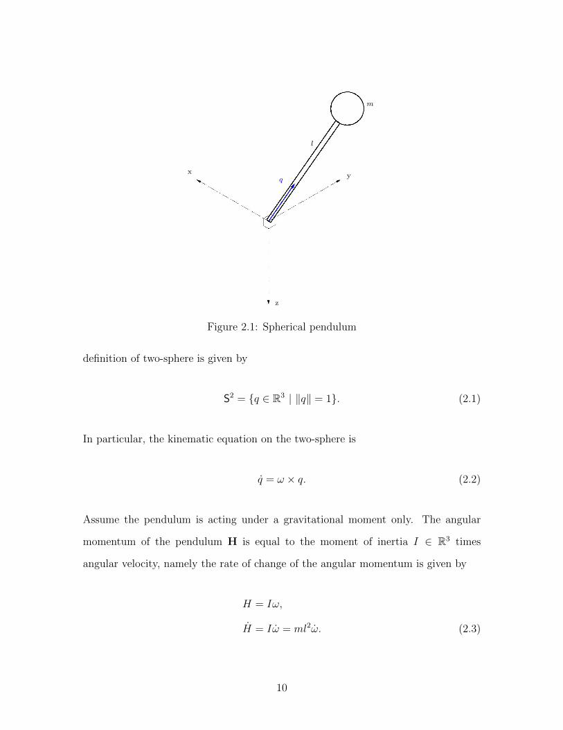
2.1 Equation of Motion

Consider a spherical pendulum supported by a fixed and frictionless pivot that is

connected to a mass m by a massless link l (Figure 2.1). The unit vector from the

pivot to the center of bob is denoted by q ∈ R3 and the corresponding angular velocity

is defined as ω ∈ R3. Notice that ω is constrained to be normal to q, i.e. ω · q = 0.

Since the pendulum lies in three dimensional space but with two dimensional degree

of freedom in rotation, the configuration of the pendulum is in the space of two-

sphere, a unit sphere in a three dimensional space, denoted by S2. The mathematical

9

l

q

m

yx

z

Figure 2.1: Spherical pendulum

definition of two-sphere is given by

S2 = q ∈ R3 | ‖q‖ = 1. (2.1)

In particular, the kinematic equation on the two-sphere is

q = ω × q. (2.2)

Assume the pendulum is acting under a gravitational moment only. The angular

momentum of the pendulum H is equal to the moment of inertia I ∈ R3 times

angular velocity, namely the rate of change of the angular momentum is given by

H = Iω,

H = Iω = ml2ω. (2.3)

10

The gravitational moment Mo is

Mo = r × F = lq ×mge3, (2.4)

where r is the position vector which equals to the length times the unit vector,

g denotes the gravitational constant and F represents the total force. Note that

e3 = [0 0 1]T represents the unit vector along the direction of gravity according to

the NED (North-East-Down) frame. Suppose that there is a control moment u ∈ R3

acting on the pivot. It is noteworthy that u is normal to q since any component of u

along q does not have any effect on the pendulum dynamics. From Newton’s second

law, the rate of change of the angular momentum is equal to the sum of the moments,

that is,

ml2ω = Mo + u = lq ×mge3 + u, (2.5)

which implies the equation of motion:

ω =g

lq × e3 +

1

ml2u. (2.6)

The projection of a vector x ∈ R3 to the plane normal to q is given by −q2x, where

the hat map · : R3 → so(3) is defined in Appendix A.

−q2x = −q × (q × x) = −[(q · x)q − (q · q)x] = −(q · x)q + x.

Considering the case x · q = 0, above equation becomes −q2x = x. Thus, for any

x ∈ R3 that is noraml to q and any vector y ∈ R3, the following property holds:

x · y = −q2x · y = −q2y · x. (2.7)

11

2.2 PD Tracking Control of a Spherical Pendulum on Two-Sphere

We first drop the integral term to design a nonlinear proportional-derivative (PD)

controller in this section. The characteristics of the two-sphere are carefully consid-

ered in the control system design, and we provide stronger convergent rate and almost

global stability for the proposed control system.

2.2.1 Error Dynamics

Desired Trajectory Suppose that a smooth desired trajectory qd ∈ R3 is given.

It satisfies

qd = ωd × qd, (2.8)

where ωd ∈ R3 is the desired angular velocity and it satisfies ωd · qd = 0. We can

further obtain the following expressions:

ωd = qd × qd,

ωd = qd × qd. (2.9)

Furthermore, the desired angular velocity is assumed to be uniformly bounded by

‖ωd‖ ≤ Bωd, Bωd > 0.

12

Error Function To measure the difference between q and qd, the error function of

the state variable is introduced as:

Ψ(q, qd) =1

2‖q − qd‖2 =

1

2(q − qd)T(q − qd)

=1

2(qTq − qTqd − qdTq + qd

Tqd)

=1

2[(‖q‖2 + ‖qd‖2)− 2q · qd]

= 1− q · qd. (2.10)

Note that ‖q‖2 = ‖qd‖2 = 1, since both of q and qd are unit vectors. Specifically, the

range of the error function is 0 ≤ Ψ(q, qd) ≤ 2.

Direction Error Vector The variation of q ∈ S2 can be written as

qε = exp(εξ)q,

where ξ = [ξ1 ξ2 ξ3]T ∈ R3 is a vector and ξ ∈ so(3) is the skew-symmetric matrix

defined as (A.1) in the appendix, which is rewritten as follows:

ξ =

0 −ξ3 ξ2

ξ3 0 −ξ1

−ξ2 ξ1 0

.

This represents the rotation of q about the axis ξ by the angle ε‖ξ‖. There is a

constraint that ξ is normal to q, i.e. ξ · q = 0. Then, the corresponding infinitesimal

variation is given by

δq =d

dε

∣∣∣∣∣ε=0

qε = ξ × q.

13

We can find the derivative of Ψ with respect to q along the direction of δq = ξ × q

for ξ ∈ R3 with ξ · q = 0 as follows:

DqΨ(q, qd) · δq =d

dε

∣∣∣∣∣ε=0

Ψ(qε, qd)

= −δq · q = −(ξ × q) · qd = (qd × q) · ξ.

Form this, the configuration error vector is defined as:

eq = qd × q. (2.11)

Note that eq · q = 0.

Angular Velocity Error Vector In order to show the difference between q and

qd, the configuration error vector eq is defined above. Similarly, the vector which links

ω and ωd is named as the angular velocity error vector and it is defined as

eω = ω + q2ωd (2.12)

= ω + q × (q × ωd)

= ω + [(q · ωd)q − (q · q)ωd]

= ω − ωd + q(q · ωd). (2.13)

It is defined such that eω · q = 0.

Proposition 2.1. The tracking error dynamics is expressed by (2.10), (2.11) and

(2.13), and they satisfies the following properties.

(i) eq · q = eω · q = 0.

(ii) ddt

Ψ(q, qd) = eq · eω.

(iii) eq · eω ≤ Bωd‖eq‖‖eω‖+ ‖eω‖2.

14

(iv) 12‖eq‖2 ≤ Ψ(q, qd) ≤ 1

2−ψ‖eq‖2, if Ψ(q, qd) ≤ ψ < 2.

Proof. Property (i) is from (2.13) and (2.11).

From (2.2) the time derivative of (2.10) is :

Ψ(q, qd) = −q · qd − q · qd

= −(ω × q) · qd − q · (ωd × qd)

= −ω · (q × qd)− ωd · (qd × q)

= (ω − ωd) · (eq). (2.14)

Also, from (2.13)

eq · eω = eq · [ω − ωd + q(q · ωd)]

= eq · (ω − ωd), (2.15)

since eq · q = 0. This shows the property (ii).

From (2.8) and (2.11), the time derivative of the direction error vector is expressed

as

eq = qd × q + qd × q

= (ωd × qd)× q + qd × (ω × q). (2.16)

Then we apply the vector identity x × (y × z) = y(x · z) − z(x · y) for x, y, z ∈ R3

and substitute (2.13) to obtain

eq = [(ωd · q)qd − (qd · q)ωd] + [(qd · q)ω − (qd · ω)q]

= (ωd · q)qd + (qd · q)(ω − ωd)− (qd · ω)q

= (ωd · q)qd + (qd · q)[eω − (q · ωd)q]− (qd · ω)q. (2.17)

15

The projection of eq to the plane normal to q is given as

−q2eq = −(ωd · q)q2qd − (qd · q)[q2eω − (q · ωd)q2q]− (qd · ω)q2q

= (ωd · q)qeq + (qd · q)eω, (2.18)

since −q2qd = −q × (q × qd) = q × eq = qeq and q2q = 0. Also, −q2eω = eω since

eω · q = 0. Again, noticing that eω is normal to q, we use (2.7) to obtain

eω · eq = eω · (−q2eq) = (ωd · q)qeq · eω + (q · qd)‖eω‖2

≤ ‖ωd‖‖eq‖‖eω‖+ ‖eω‖2

≤ Bωd‖eq‖‖eω‖+ ‖eω‖2,

which shows property (iii).

The last property is about the bounds of the error function. Define a constant ψ

and D = q ∈ S2 | Ψ(q, qd) ≤ ψ < 2. From (2.10), we have Ψ(q, qd) = 1 − cos(θ)

where θ ∈ S1 is the angle between q and qd. This yields:

0 ≤ 1− cos(θ) ≤ ψ,

We rearrange the equation to have

1

2≤ 1

1 + cos θ≤ 1

2− ψ,

which yields

1

2‖eq‖2 ≤ 1

1 + cos θ‖eq‖2 ≤ 1

2− ψ‖eq‖2.

From (2.11), we have ‖eq‖2 = sin2 θ. Therefore, 11+cos θ

‖eq‖2 = 1 − cos θ = Ψ(q, qd),

16

which shows property (iv).

2.2.2 Control System Design

Using the properties derived in previous section, we design a continuous feedback

controller that exponentially stabilizes the desired eqilibium.

Proposition 2.2. Consider the system is given by (2.6) and (2.2) with a tracking

command given by (2.8). The control input is designed as follows:

u = ml2[−kωeω − kqeq − q2ωd − q(q · ωd)−g

lq × e3], (2.19)

where kω and kq are positive constants. The following properties are satisfied by the

control input:

(i) Equilibrium configuration is given by (q, ω) = (±qd, ωd) .

(ii) The desired equilibrium point (qd, ωd) is almost globally exponentially stable

with an estimate of the region of attraction given by

Ψ(q(0), qd(0)) ≤ ψ < 2, (2.20)

‖eω(0)‖2 ≤ 2kq(ψ −Ψ(q(0), qd(0))). (2.21)

(iii) The undesired equilibrium (−qd, ωd) is unstable.

The controller we present in (2.19) is expressed in terms of unit vector q, angular

velocity ω which is much simpler than using complicated trigonometric functions.

More importantly, the manifold converges to unstable equilibrium has less dimension

than the tangent bundle of the configuration space of S2. Therefore, almost global

exponential stability is achieved.

17

Proof. Property (i) is from the fact that the zero equilibrium of the tracking errors is

(eq, eω) = (0, 0).

To find the region of attraction, define

U =1

2eω · eω + kqΨ(q, qd).

A Lyapunov candidate is specified as

V =1

2eω · eω + kqΨ(q, qd) + ceq · eω. (2.22)

for a constant c satisfying

c < min√kq,

√2kq

2− ψ1

,4kqkω

(kω −Bωd)2 + 4kq. (2.23)

Then, from property (iv) of Proposition 2.1, we obtain

1

2eω · eω +

1

2kq‖eq‖2 − c‖eq‖‖eω‖ ≤ V ≤

1

2eω · eω +

1

2− ψ1

kq‖eq‖2 + c‖eq‖‖eω‖.

This equation can be further rewritten as

zTM1z ≤ V ≤ zTM2z,

λmin(M1)‖z‖2 ≤ V ≤ λmax(M2)‖z‖2. (2.24)

where z =

‖eq‖‖eω‖

∈ R2, M1 = 12

kq −c

−c 1

∈ R2×2, and M2 = 12

2kq2−ψ1

c

c 1

∈R2×2. The matrices M1 and M2 are guaranteed to be positive definite as long as the

constant c satisfying(2.23).

Next, we will prove the time-derivative of the Lyapunov function is negative def-

inite. To show this, we start from deriving the time-derivative of eω. The time

18

derivative of (2.13) is

eω = ω − ωd + q(q · ωd) + q(q · ωd) + q(q · ωd). (2.25)

Substituting (2.19) into (2.6), we have

ω = −kωeω − kqeq + ωd − q(q · ωd). (2.26)

Then substituting (2.26) into (2.25), we obtain

eω = −kωeω − kqeq + q(q · ωd) + q(q · ωd). (2.27)

From the property (ii) of Proposition 2.1, and (2.27), the time-derivative of V is

given by:

V = eω · eω + kqeq · eω + ceq · eω + ceq · eω

= (eω + ceq) · (−kωeω − kqeq) + kqeq · eω + ceq · eω

= −kω‖eω‖2 − ckωeq · eω − ckq‖eq‖2 + ceq · eω

≤ −kω‖eω‖2 + ckω‖eq‖‖eω‖ − ckq‖eq‖2 + ceq · eω. (2.28)

Notice that eω · q = eq · q = 0 since both of eq and eω are normal to q. Moreover, By

applying property (iii) of propositon 1, the time-derivative of Lyapunov function is

bounded by

V ≤ −[(kω − c)‖eω‖2 − c(kω −Bωd)‖eq‖‖eω‖+ ckq‖eq‖2] = −zTQz

≤ −λmin(Q)‖z‖2, (2.29)

19

where the matrix Q ∈ R2×2 is defined by

Q =

ckq − c(kω+Bωd)2

− c(kω+Bωd)2

kω − c

. (2.30)

The matrix Q is positive definite if the leading principle minors of Q are positive,

that is,

ckq(kω − c)−c2(kω −Bωd)

2

4> 0, (2.31)

which implies the last condition in (2.23),

c <4kqkω

(kω −Bωd)2 + 4kq. (2.32)

We now conclude that the zero equilibrium is exponentially stable under the designed

control input.

To show (iii), The undesired equilibrium (q, ω) = (−qd, ωd) implies eq = eω = 0

and Ψ(q, qd) = Ψ(−qd, qd) = 2, thus the Lyapunov function, i.e., (2.22) equals to 2kq.

And we can further define

W = 2kq − V = −1

2eω · eω + (2kq − kqΨ(q, qd))− ceq · eω, (2.33)

Now, at the undesired equilibrium W = 0, we can write

W ≥ −1

2‖eω‖2 + kq(2−Ψ(q, qd))− c‖eq‖‖eω‖, (2.34)

We can choose q that is arbitrary close to −qd such that 2−Ψ(q, qd) is still positive.

If ‖eω‖ is sufficiently small, we know W > 0 at some points, i.e., at any small

20

neighborhood of (−qd, 0), there exists a domain such that

W = −V > 0. (2.35)

As stated by Theorem 4.3 of [43], the undesired equilibrium is unstable. Property

(iii) is verified.

It has been shown that a lower dimensional manifoldMr can be defined such that

closed-loop solutions starting inMr will converge to the undesired equilibrium and all

other solutions converges to the desired equilibrium [14]. Particularly, the dimension

of Mr is less than the tangent space of the configuration manifold. Therefore, the

desired equilibrium is exponentially stabilized for almost every initial condition except

Mr.

2.3 PID Tracking Control of a Spherical Pendulum on Two-Sphere

All of the control systems are subjected to disturbances and uncertainties. If we

consider the disturbances and uncertainties, the equation of motion of the pendulum

system now can be written as:

ω =g

lq × e3 +

1

ml2u− q2∆, (2.36)

where ∆ is the fixed perturbation.

In the PD controller, the proportional term eq is about present error, while the

derivative error eω stands for the prediction of future error. Here we introduce the

integral term, representing the accumulation of past error, denoted by

ei =

∫ t

0

(ceq + eω)dτ. (2.37)

Using the properties derived before, we select a continuous feedback controller

21

that stabilizes the desired equilibrium.

Proposition 2.3. Consider the system is given by Eq. (2.36) and (2.2) with a

tracking command given at Eq. (2.8). The control input is designed as follows:

u′ = ml2[−kωeω − kqeq + kiq2ei − q2ωd − q(q · ωd)−

g

lq × e3], (2.38)

where kω, kq and ki are positive constants. The following properties are satisfied by

the PID controller: the zero equilibrium of the tracking errors, namely (eq, eω, ei) =

(0, 0, ∆ki

) is stable. The present controller is robust with fixed perturbation ∆ with

the aid of integrator ei.

Proof. A Lyapunov candidate is specified as

V ′ = 1

2eω · eω + kqΨ(q, qd) + ceq · eω +

1

2ki(kiei −∆)2. (2.39)

Then, applying property (iv) of Proposition 2.1 into (2.22) leads to

V ′ ≥ 1

2‖eω‖2 +

1

2kq‖eq‖2 − c‖eq‖‖eω‖+

1

2ki(kiei −∆)2

= zTM1z +1

2ki(kiei −∆)2,

Thus, the Lyapunov function V ′ is guaranteed to be positive definite.

V ′ ≥ λmin(M1)‖z‖2 +1

2ki(kiei −∆)2. (2.40)

Substitute (2.38) into (2.36) and then apply the new form of ω to (2.25). We have

eω = −kweω − kqeq + kiq2ei + kiq(q · ei) + q(q · ωd)− q2∆. (2.41)

22

And the time-derivative of V ′ is expressed as

V ′ = eω · eω + kqeq · eω + ceq · eω + ceq · eω +1

ki(kiei −∆) · (kiei)

= (eω + ceq)eω + kqeq · eω + ceq · eω + (kiei −∆) · (ceq + eω)

= (eω + ceq)[−kweω − kqeq − kiei + kiq(q · ei) + q(q · ωd)− q(q ·∆) + ∆]

+ kqeq · eω + ceq · eω + ckiei · eq + kiei · eω − c∆ · eq −∆ · eω.

Using eq · q = eω · q = 0, the related terms can be eliminated. Finally, we have

V ′ = (eω + ceq)[−kweω − kqeq − kiei + ∆] + kqeq · eω + ceq · eω + ckiei · eq

+ kiei · eω − c∆ · eq −∆ · eω

= −kweω · eω − ckweq · eω − ckqeq · eq + ceq · eω

= V . (2.42)

All of the terms with the fixed perturbation are annihilated, hence the time-derivative

of the Lyapunov function of PID controller is exactly same with our previous work

about the PD tracking control. Since there exists a new state ei in the PID case, V

is semi-negative definite and we can only conclude that the equilibrium (eq, eω, ei) =

(0, 0, ∆ki

) is stable.

2.4 Numerical Example

We present numerical examples for a spherical pendulum on S2 corresponding to

Proposition 2.2 and Proposition 2.3. The initial conditions q = [0 0 1]T and ω =

[0 0 0]T imply that the pendulum is in rest at the stable equilibrium. The length of

the link and weight of the bob is 0.2m and 1kg, respectively. In addition, the control

gain are chosen as kq = 10 and kw = 10.1. The desired direction of the pendulum qd

23

can be a continuous function of time and must satisfies ‖qd‖T = 1 since it is a unit

vector, thus we select

qd = [cos(αt) cos(βt) cos(αt) sin(βt) sin(αt)]T, (2.43)

where α = 0.5 and β = 2. The corresponding numerical distributions are described

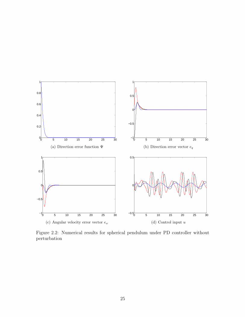
at Figure 2.2.

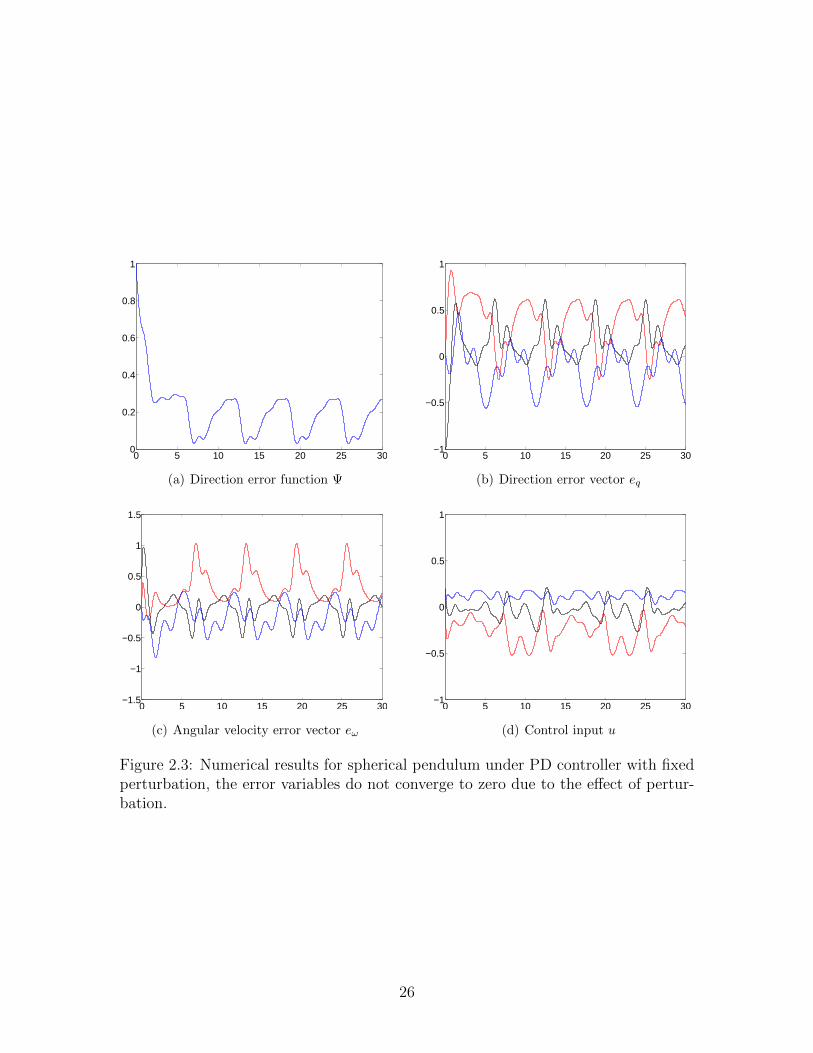
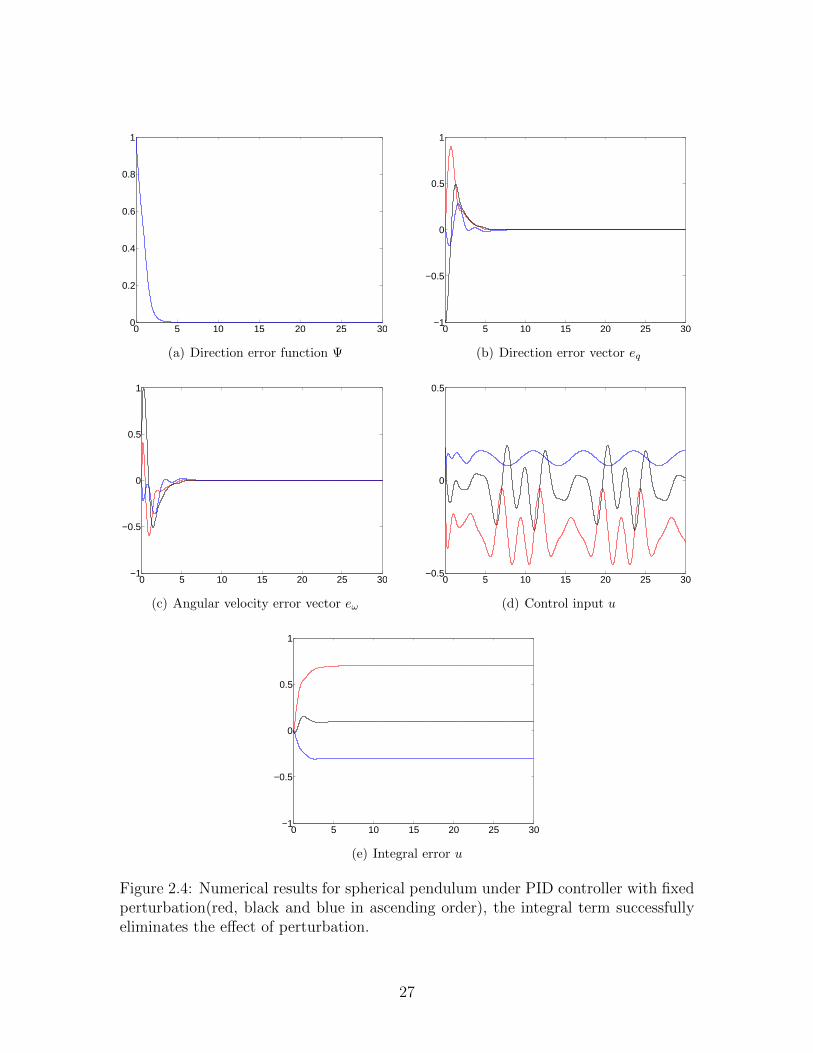
The feature of PID controller is eliminating the effect of fixed perturbation where

∆ = [7 1 −3]T. We then add the perturbation and execute the simulation on PD and

PID controller so the effect of integral term can be distinctly observed. The numerical

results for PD and PID controller with respect to fixed perturbation are illustrated

at Figure 2.3 and Figure 2.4, respectively.

24

0 5 10 15 20 25 300

0.2

0.4

0.6

0.8

1

(a) Direction error function Ψ

0 5 10 15 20 25 30−1

−0.5

0

0.5

1

(b) Direction error vector eq

0 5 10 15 20 25 30−1

−0.5

0

0.5

1

(c) Angular velocity error vector eω

0 5 10 15 20 25 30−0.5

0

0.5

(d) Control input u

Figure 2.2: Numerical results for spherical pendulum under PD controller withoutperturbation

25

0 5 10 15 20 25 300

0.2

0.4

0.6

0.8

1

(a) Direction error function Ψ

0 5 10 15 20 25 30−1

−0.5

0

0.5

1

(b) Direction error vector eq

0 5 10 15 20 25 30−1.5

−1

−0.5

0

0.5

1

1.5

(c) Angular velocity error vector eω

0 5 10 15 20 25 30−1

−0.5

0

0.5

1

(d) Control input u

Figure 2.3: Numerical results for spherical pendulum under PD controller with fixedperturbation, the error variables do not converge to zero due to the effect of pertur-bation.

26

0 5 10 15 20 25 300

0.2

0.4

0.6

0.8

1

(a) Direction error function Ψ

0 5 10 15 20 25 30−1

−0.5

0

0.5

1

(b) Direction error vector eq

0 5 10 15 20 25 30−1

−0.5

0

0.5

1

(c) Angular velocity error vector eω

0 5 10 15 20 25 30−0.5

0

0.5

(d) Control input u

0 5 10 15 20 25 30−1

−0.5

0

0.5

1

(e) Integral error u

Figure 2.4: Numerical results for spherical pendulum under PID controller with fixedperturbation(red, black and blue in ascending order), the integral term successfullyeliminates the effect of perturbation.

27

Chapter 3 Vision-based Spacecraft Attitude Control on

SO(3)

This chapter presents a control strategy to rotate single spacecraft by using the in-

formation provided by a vision system. To be more specific, we select two distinct

point objects as visual features, and use optical devices to obtain the line-of-sight

(LOS) measurements to determine the absolute attitude of the spacecraft. The LOS

observation is represented by a unit vector in two-sphere, which is analogous to the

control system of a spherical pendulum we have presented in the preceding chapter.

We will explore the advantage the LOS observations in the next chapter to develop

a relative attitude control system for multiple spacecrafts.

3.1 Problem Formulation

3.1.1 Attitude Dynamics on SO(3)

Consider a spacecraft modeled as a rigid body. The origin of the body-fixed frame

B are defined at the mass center of the spacecraft. A inertial reference frame or

world frame W is also defined. Each frame is is constructed by three orthogonal unit

basis vectors ordered according to the right-hand rule. A rotation matrix R ∈ SO(3)

represents the physical attitude of the spacecraft where SO(3) is the special orthogonal

group which denotes the set of all rotation matrices, that is

SO(3) = R ∈ R3×3 | RTR = I, det(R) = 1. (3.1)

28

Spacecraft

Object 1

Object 2

s1 = Rb1

s2 = Rb2

Figure 3.1: Problem definition: directions from spacecraft toward two distinct ob-jects are given by s1 and s2 ∈ S2 with respect to the inertial reference frame. Thecorresponding line-of-sight measurements, b1 and b2 ∈ S2 are represented with respectto the body-fixed frame. They are related by the rotation matrix R representing theattitude of the spacecraft.

The rotation matrix represents the linear transformation from the body-fixed frame to

the inertial reference frame. Furthermore, its transpose indicate the inverse mapping

because of the orthogonality RT = R−1,

W r = R(Br), Br = RT(W r), (3.2)

where Br is a vector quantity r with respected to the body fixed frame and W r is

the same vector with respect to the inertial reference frame. Notice that the full

transformation between the two coordinate system also includes the the position

transformation. However, the discussion about relative position is neglected in this

thesis since we only care about the relative orientation.

29

The equation of motions for the spacecraft are given by

JΩ + Ω× JΩ = u, (3.3)

R(t) = R(t)Ω, (3.4)

where J ∈ R3×3 is the inertia matrix, Ω ∈ R3 represents the angular velocity of

the body-fixed frame with respect to the inertial reference frame expressed in the

body-fixed frame, and u denotes the total external moments applied to the aircraft

expressed in the body-fixed frame. Assume that the desired angular velocity is uni-

formly bounded. In other words, for any t ≥ 0, there exists a known constant BΩd > 0

such that

‖Ω(t)‖ ≤ BΩd. (3.5)

3.1.2 Vision-Based Attitude Control Problem

Suppose that there are two distinct objects, such as distant stars, whose location in

the inertia reference frame is available. Let s1, s2 ∈ R3 be the unit vectors showing

the direction from the spacecraft to the first object and the second object expressed

in the inertial reference frame, respectively. Since each of these two vectors has unit

length, they lie in the two-sphere S2. The relative positions of objects with respect

to the spacecraft are assumed to be fixed and they are non-parallel with each other,

i.e., the following properties are satisfied:

s1 = s2 = 0, s1 × s2 6= 0. (3.6)

Assume the spacecraft is equipped with an onboard camera which can capture the

direction to two distinct objects. These two line-of-sight (LOS) measurements from

spacecraft toward the objects are defined as b1, b2 ∈ S2 (Figure 3.1). Since s1, s2 and

30

b1, b2 are referred to the same vectors with respect to different reference frames, they

are related by the rotation matrix. From (3.2), we can write

s1 = R(t)b1(t), s2 = R(t)b2(t), (3.7)

b1(t) = R(t)Ts1, b2(t) = R(t)Ts2. (3.8)

Additionally, (3.4) shows that

R(t)T = (R(t)Ω)T = ΩTR(t)T = −ΩR(t)T. (3.9)

From (3.9), (3.8) and the assumption si = 0, we can obtain the kinematic equations

for b1, b2,

bi(t) = R(t)Tsi +R(t)Tsi = −ΩR(t)Tsi

= −Ωbi(t) = −Ω(t)× bi(t) = bi(t)× Ω(t), (3.10)

for i ∈ 1, 2.

Suppose that the desired attitude trajectory Rd(t) ∈ SO(3) is given, It satisfies

the following kinematic equation

Rd(t) = Rd(t)Ωd(t), (3.11)

where Ωd(t) ∈ SO(3) is the desired angular velocity. The corresponding desired line-

of-sight measurements are given by

bid(t) = Rd(t)Tsi, i = 1, 2. (3.12)

Similar with (3.10), the kinematic equations for desired line-of-sight measurements

31

are denoted by

bid(t) = bid(t)× Ωd(t). (3.13)

According to the rigid body assumption, the angle between b1 and b2 is always

same as the angle between s1 and s2 and the angle between .

b1(t) · b2(t) = R(t)Ts1 ·R(t)Ts2 = [R(t)Ts1]T[R(t)Ts2]

= sT1R(t)R(t)Ts2 = sT1 s2 = s1 · s2.

Since b1d and b2d are elements of b1 and b2, respectively, the foregoing property is also

valid, i.e., b1d(t) · b2d(t) = s1 · s2.

The goal is to design a control input u in terms of the line-of-sight measure-

ments b1(t), b2(t) and the angular velocity Ω(t) such that the spacecraft attitude R(t)

asymptotically follows the desired attitude Rd(t).

3.2 Almost Global Exponential Tracking Control on SO(3)

In order to let the spacecraft follow the desired trajectory, the desired attitude is

assigned, and the difference of the current and desired attitude are characterized by

smooth positive function called error function. Moreover, we are able to define error

vectors, representing the difference of current angular velocity and LOS measurements

between the desired ones, from the tangent space of the error function since we are

dealing with a nonlinear manifold. We then construct the controller directly by

the error vectors based on Lyapunov stability analysis so that the spacecraft can

exponentially track the desired motion even though the initial attitude errors are

significantly large.

32

3.2.1 Error Variables

First, we choose error functions that represent the distance between the desired atti-

tude and the current attitude. The configuration error functions are defined as

Ψ1(b1, b1d) = 1− b1 · b1d , Ψ2(b2, b2d) = 1− b2 · b2d , (3.14)

Ψ(b1, b2, b1d , b2d) = kb1Ψ1(b1, b1d) + kb2Ψ2(b2, b2d). (3.15)

For simplicity, hereafter we will use Ψ and Ψi as the short note of Ψ(b1, b2, b1d , b2d) and

Ψi(bi, bid), respectively. For each object i, Ψi refers to the corresponding error of LOS

measurements while Ψ involves the LOS error of the complete control system. Once

the error of each line-of-sight measurements goes to zero, the error of the complete

control system goes to zero as well.

Substituting (3.8), the error function Ψi can be written as

Ψi(R) = 1−RTsi ·RTd si. (3.16)

Since we have the assumption that si is fixed and Rd is given, Ψi can be considered

as a function of R. Furthermore, the infinitesimal variation of a rotation matrix R

can be expressed in terms of the exponential map as follows

δR =d

dε

∣∣∣∣∣ε=0

R exp(εη) = Rη, (3.17)

for a vector η ∈ R3. Thus, from (3.16) and substituting (3.17), the variation of Ψi is

expressed by

δΨi =d

dε

∣∣∣∣∣ε=0

Ψi(R exp(εη)) = −(Rη)Tsi ·RTd si = ηbi · bid = bid · (η × bi)

= η · (bi × bid). (3.18)

33

According to (3.18), the configuration error vectors are defined as

eb1 = b1 × b1d , eb2 = b2 × b2d , (3.19)

eb = kb1eb1 + kb2eb2 . (3.20)

Notice that since bi and bid are unit vectors, the magnitude of ebi is bounded, i.e.

‖ebi‖ ≤ 1, which leads to

‖eb‖ ≤ kb1‖eb1‖+ kb2‖eb2‖ ≤ kb1 + kb2 . (3.21)

The angular velocity error vector is defined as

eΩ = Ω− Ωd. (3.22)

The properties of error variables mentioned above are summarized as follows.

Proposition 3.1. The error variables (3.14)-(3.22) satisfy the following properties

(i) ddt

Ψi(bi, bid) = ebi · eΩ for i = 1, 2.

(ii) ‖eb‖ ≤ (kb1 + kb2)‖eΩ‖+BΩd‖eb‖.

(iii) Define a matrix K ≡= kb1s1sT1 + kb2s2s

T2 ∈ R3×3 and let g1, g2 ∈ R be two pos-

itive eigenvalues of K. If Ψ < ψ < h1 ≡ 2 ming1, g2, the following inequality

holds:

h1

h2 + h3

‖eb‖2 ≤ Ψ ≤ h1h4

h5(h1 − ψ)‖eb‖2, (3.23)

34

where the constants are defined as

h1 = 2 ming1, g2,

h2 = 4 max(g1 − g2)2, g21, g

22,

h3 = 4(g1 + g2)2,

h4 = 2(g1 + g2),

h5 = 4 ming21, g

22,

Proof. From (3.14) and (3.10), we can show (i) by

Ψi = −bi · bid − bi · bid

= −(bi × Ω) · bid − bi · (bid × Ωd)

= −Ω(bid × bi)− Ωd(bi × bid)

= (Ω− Ωd) · (bi × bid)

= eΩ · ebi ,

and the time-derivative of Ψ is defined by

Ψ = kb1Ψ1 + kb2Ψ2 = kb1eΩ · eb1 + kb2eΩ · eb2 = eΩ · (kb1eb1 + kb1eb1) = eΩ · eb.

35

From ebi = bi × bid , ebi is given by

ebi = bi × bid + bi × bid

= (bi × Ω)× bid + bi × (bid × Ωd)

= −bid × (bi × Ω) + bi × (bid × Ωd)

= −[bi(bid · Ω)− Ω(bid · bi)] + bid(bi · Ωd)− Ωd(bi · bid)

= (Ω− Ωd)(bid · bi) + bid(bi · Ωd)− bi(bid · Ω). (3.24)

Substituting Ω = eΩ − Ωd then applying (A.3) in the appendix, above equation

becomes

ebi = eΩ(bid · bi) + bid(bTi )Ωd − bi(bTid)(eΩ + Ωd)

= eΩ(bid · bi) + [bid(bTi )− bi(bTid)]Ωd − bi(bTid)eΩ

= eΩ(bid · bi)− bi(bid · eΩ) + (bi × bid)Ωd

= bid × (eΩ × bi) + (bi × bid)× Ωd

= −bid × (bi × eΩ) + ebi × Ωd, (3.25)

which leads to

‖ebi‖ ≤ ‖eΩ‖+BΩd‖ebi‖, (3.26)

and

‖eb‖ ≤ kb1(‖eΩ‖+BΩd‖eb1‖) + kb2(‖eΩ‖+BΩd‖eb2‖) = (kb1 + kb2)‖eΩ‖+BΩd‖eb‖,

(3.27)

where ‖eb‖ = kb1‖eb1‖+ kb2‖eb2‖. Hence property (ii) is proved.

36

To show property (iii), we introduce alternative expressions for Ψ and eb

Ψ = kb1Ψ1 + kb2Ψ2

= kb1(1− b1 · b1d) + kb2(1− b2 · b2d)

= kb1 + kb2 − kb1bT1 b1d − kb2bT2 b2d

= kb1 + kb2 − tr[kb1b1bT1d

+ kb2b2bT2d

]

= kb1 + kb2 − tr[kb1(RTs1)(RT

d s1)T + kb2(RTs2)(RT

d s2)T]

= kb1 + kb2 − tr[kb1(RTs1)(sT1 )Rd + kb2(R

Ts2)(sT2 )Rd]

= kb1 + kb2 − tr[RT(kb1s1sT1 + kb2s2s

T2 )Rd]

, kb1 + kb2 − tr[RTKRd], (3.28)

where we just appied xTy = tr[xyT] for any x, y ∈ R3. Let µi ∈ R and νi ∈ R3 be

the i-th eigenvalue and normalized eigenvector of K, respectively. According to the

spectral theorem addressed in appendix B, the matrix K can be factored to

K ≡ UGUT, (3.29)

where U = [ν1 ν2 ν3] ∈ SO(3), G = diag[µ1 µ2 µ3] ∈ R3×3. In particular, it is ordered

that µ3 = 0 and ν3 = ν1 × ν2 such that U lies in SO(3). Alternatively, we have

kb1 + kb2 = tr[K] = tr[UGUT] = tr[GUTU ] = tr[G]. (3.30)

The first equality comes fromK = kb1s1sT1 +kb2s2s

T2 , where tr[sis

Ti ] = sTi si = ‖si‖2 = 1

for i = 1, 2. The rest comes from the trace identities tr[xy] = tr[yx] = tr[xTyT] =

tr[yTxT] for any x, y ∈ R3.

37

Thus, using (3.30), we can rewrite (3.28) as

Ψ = tr[G]− tr[RT(UGUT)Rd]

= tr[G]− tr[(RTdUGU

T)R]

= tr[G]− tr[(GUTR)(RTdU)] (3.31)

= tr[G(I − UTRRTdU)]. (3.32)

This is an alternative expression of Ψ.

From (3.31), we differentiate Ψ with respect to R along the direction δR = Rη to

obtain

DRΨ ·Rη = −tr[GUTRηRTdU ] = −tr[(ηRT

dU)(GUTR)] = −tr[(RTdKR)η]. (3.33)

From (A.9), we have

DRΨ ·Rη = ηT[RTdKR− (RT

dKR)T]∨ (3.34)

= η · [RTd (kb1s1s

T1 + kb2s2s

T2 )R−RT(kb1s1s

T1 + kb2s2s

T2 )Rd]

∨

= η · [kb1(RTd s1s

T1R) + kb2(R

Td s2s

T2R)− kb1(RTs1s

T1Rd)− kb2(RTs2s

T2Rd)]

∨

= η · [kb1(b1dbT1 ) + kb2(b2db

T2 )− kb1(b1b

T1d

)− kb2(b2bT2d

)]∨

= η · [kb1(b1dbT1 − b1b

T1d

) + kb2(b2dbT2 − b2b

T2d

)]∨. (3.35)

Substituting (A.3),

DRΨ ·Rη = η · [kb1( b1 × b1d)∨ + kb2( b2 × b2d)∨]

= η · [kb1(b1 × b1d) + kb2(b2 × b2d)]

= η · (kb1eb1 + kb2eb2)

= η · eb. (3.36)

38

Comparing (3.34) with (3.36), we obtain

eb = [RTdKR− (RTKRd)]

∨, (3.37)

which is an alternative expression of eb.

These alternative expressions can be compared with [44] to show the third prop-

erty. The properties developed in [44] are summarized as follows

Φ =1

2tr[F (I − P )], (3.38)

eP =1

2(FP − PTF )∨, (3.39)

h1

h2 + h3

‖eP‖2 ≤ Φ ≤ h1h4

h5(h1 − ψ)‖eP‖2, (3.40)

where P ∈ SO(3), F = diag[f1, f2, f3] and the constants hi are given by

h1 = minf1 + f2, f2 + f3, f3 + f1,

h2 = max(f1 − f2)2, (f2 − f3)2, (f3 − f1)2,

h3 = max(f1 + f2)2, (f2 + f3)2, (f3 + f1)2,

h4 = maxf1 + f2, f2 + f3, f3 + f1,

h5 = min(f1 + f2)2, (f2 + f3)2, (f3 + f1)2,

and it is assumed that Φ < ψ < h1.

After comparing (3.38) with (3.32), we let F = 2G and P = UTRRTdU so Φ = Ψ.

39

Then (3.39) is equivalent to

eP = GUTRRTdU − UTRdR

TUG

= (UTU)GUTRRTdU − UTRdR

TUG(UTU)

= UT(UGUTRRTd −RdR

TUGUT)U

= UT(KRRTd −RdR

TK)U, (3.41)

where we have multiplied the identity matrix I = UTU ∈ R3. Similarly, we now

multiply I = RdRTd and then apply (A.4) so that

eP = UT[(RdRTd )KRRT

d −RdRTK(RdR

Td )]U

= UTRd(RTdKR−RTKRd)R

TdU

= (UTRd)eb(UTRd)

T

= (UTRdeb)∧. (3.42)

Thus, eP = UTRdeb, which implies that ‖eP‖ = ‖eb‖ since U and Rd are all orthogonal

matrices. From (3.40), The bounds of Ψ are given as

h1

h2 + h3

‖eb‖2 ≤ Φ ≤ h1h4

h5(h1 − ψ)‖eb‖2.

In particular, f1 = 2kb1 , f1 = 2kb2 , and f3 = 0, the constants hi now are valued as

h1 = min2kb1 , 2kb2,

h2 = max4(kb1 − kb2)2, 4k2b2, 4k2

b1,

h3 = 4(kb1 + kb2)2,

h4 = 2(kb1 + kb2),

h5 = min4k2b2, k2

b1,

40

which shows (iii). Notice that the eigenvalues u1 and u2 defined in the Proposition

3.1 equal to kb1 and kb2 , respectively, according to the spectral theory.

3.2.2 Control System Design

Based on the properties we derived in the previous section, a control input is designed.

By applying the designed control input, the equilibrium of the controlled system is

guaranteed to have exponential convergence.

Proposition 3.2. Consider the dynamic system (3.3) and (3.4) on SO(3) with the

desired trajectory (3.11) and (3.12), a control input is chosen as

u = −eb − kΩeΩ + ΩdJ(eΩ + Ωd) + JΩd, (3.43)

then the following properties are secured:

(i) There are four equilibrium configurations, give by

(R,Ω) ∈ (Rd,Ωd), (UD1UTRd,Ωd), (UD2U

TRd,Ωd), (UD3UTRd,Ωd), (3.44)

where D1 = diag[1,−1,−1], D2 = diag[−1, 1,−1], and D3 = diag[−1,−1, 1]

are diagonal matrices with trace equals to -1 and U ∈ SO(3) which is already

defined in (3.29).

(ii) The desired equilibrium (Rd,Ωd) is almost globally exponentially stable, with

an estimate of region of attraction given by

Ψ(0) ≤ ψ < h1, (3.45)

‖eΩ(0)‖2 ≤ 2

λM(J)(ψ −Ψ(0)), (3.46)

where Ψ(0) ≡ Ψ(b1(0), b2(0), b1d(0), b2d(0)) and λM(J) denotes the maximum

41

eigenvalue of J .

(iii) The remaining three undesired equilibrium configurations are unstable.

Without using any IMU sensors, two distinct pointing direction, referring to LOS

measurements, are used to determine the absolute attitude. And the control input

is directly expressed by the LOS measurements. Besides, by showing the instability

of three undesired configuration equilibrium, the region of attraction of the desired

equilibrium is almost global.

Proof. The equilibrium configurations locate at (eΩ, eb) = (0, 0). Since eΩ = Ω− Ωd,

we know that eΩ = 0 leads to Ω = Ωd. As for eb = 0, recall (3.37) to write

eb = [RTdKR−RTKRd]

∨

= [RTdKR(RT

dRd)− (RTdRd)R

TKRd]∨

= [RTd (KRRT

d −RdRTK)Rd]

∨

= RTd [K(RRT

d )− (RRTd )TK]Rd∨, (3.47)

which implies that

K(RRTd )− (RRT

d )TK = 0. (3.48)

In [29], it has been show that (3.48) reveals

RRTd ∈ I, UD1U

T, UD2UT, UD3U

T (3.49)

where D1 = diag[1,−1,−1], D2 = diag[−1, 1,−1], and D3 = diag[−1,−1, 1]. Hence

we are now able to show the eqauilibria in terms of R and Ω, which is (i).

42

To show the exponential stability, We first rewrite (3.3) as follows,

JΩ + Ω× JΩ− JΩd = u− JΩd, (3.50)

which leads to

JeΩ = J(Ω− JΩd) = −Ω× JΩ− JΩd + u. (3.51)

Substituting eΩ = Ω− Ωd and (A.2), we have

JeΩ = −(eΩ + Ωd)× J(eΩ + Ωd)− JΩd + u

= −eΩ × J(eΩ + Ωd)− Ωd × J(eΩ + Ωd)− JΩd + u

= [J(eΩ + Ωd)]∧eΩ − ΩdJ(eΩ + Ωd)− JΩd + u.

Now substitute the control input into this equation, and the error dynamics for the

angular velocity is given by

JeΩ = [J(eΩ + Ωd)]∧eΩ − eb − kΩeΩ. (3.52)

To show the exponential stability, we first define

U =1

2eΩ · JeΩ + Ψ,

notice that U ≥ Ψ. Then, the time-derivative of U is given by

U = eΩ · JeΩ + Ψ

= eΩ · ([J(eΩ + Ωd)]∧eΩ − eb − kΩeΩ) + eΩ · eb

= −kΩ‖eΩ‖2,

43

which implies that U(t) is a non-increasing function. To specify the initial condition

of U , we have

U(0) =1

2eΩ(0) · JeΩ(0) + Ψ(0) ≤ 1

2λM(J)‖eΩ(0)‖2 + Ψ(0). (3.53)

Substituting (3.45) and (3.46) to (3.53) yields to

U(0) ≤ 1

2λM(J)‖eΩ(0)‖2 + Ψ(0)

≤ 1

2λM(J)

2

λM(J)(ψ −Ψ(0)) + Ψ(0) = ψ. (3.54)

Since U(t) is non-increasing, the value of U(t) must be less or equal than U(0) and

we already know U(t) ≥ Ψ(t). Combine (3.45) and (3.54) to obtain

Ψ(t) ≤ U(t) ≤ U(0) ≤ ψ < h1.

This inequality implies that Ψ(t) < h1 for all t > 0, and (3.40) is also satisfied.

The Lyapunov candidate is given as

V =1

2eΩ · JeΩ + Ψ + ceΩ · eb = U + ceΩ · eb, (3.55)

where c is a positive constant. Notice that

λm(J)‖eΩ‖2 ≤ eΩT · JeΩ ≤ λM(J)‖eΩ‖2 (3.56)

−c‖eΩ‖‖eb‖ ≤ ceΩ · eb ≤ c‖eΩ‖‖eb‖. (3.57)

By combining the inequalities, (3.56), (3.57) with (3.40) we can obtain the upper and

44

lower bounds of V as follows

V ≤ 1

2λM(J)‖eΩ‖2 +

h1h4

h5(h1 − ψ)‖eb‖2 + c‖eΩ‖‖eb‖,

V ≥ 1

2λm(J)‖eΩ‖2 +

h1

h2 + h3

‖eb‖2 − c‖eΩ‖‖eb‖,

which can be written in the following matrix form

zTM1z ≤ V ≤ zTM2z, (3.58)

where z =

‖eb‖‖eΩ‖

, M1 = 12

2h1h2+h3

−c

−c λm(J)

and M2 = 12

2h1h4h5(h1−ψ)

c

c λM(J)

.

To guarantee M1 and M2 to be positive definite, we have

c < min

√2h1λm(J)

h2 + h3

,

√2h1h4λM(J)

h5(h1 − ψ) (3.59)

The time-derivative of V is given as

V = U + ceΩ · eb + ceΩ · eb

= −kΩ‖eΩ‖2 + ceΩ · eb + ceΩ · eb. (3.60)

To obtain the upper bound of eΩ · eb, we first use (3.52) to have

J−1JeΩ = eΩ = J−1[J(eΩ + Ωd)]∧eΩ − J−1eb − kΩJ

−1eΩ,

45

and then

eΩ · eb = J−1[J(eΩ + Ωd)]∧eΩ · eb − J−1‖eb‖2 − kΩJ

−1eΩ · eb

≤ λM(J−1)‖[λM(J)(eΩ + Ωd)]∧eΩ‖‖eb‖ − λm(J−1)‖eb‖2 + kΩλm(J−1)‖eΩ‖‖eb‖

≤ ‖eb‖λm(J)

(‖λM(J)‖eΩ‖2 + λM(J)BΩd‖eΩ‖)−1

λM(J)‖eb‖2 + kΩ

1

λm(J)‖eΩ‖‖eb‖

=‖eb‖λm

(‖λM‖eΩ‖2 + λMBd‖eΩ‖)−1

λM‖eb‖2 + kΩ

1

λm‖eΩ‖‖eb‖. (3.61)

Furthermore, by using property (ii) of Proposition 3.1, the upper bound of eΩ · eb is

given by

‖eΩ‖‖eb‖ ≤ (kb1 + kb2)‖eΩ‖2 +BΩd‖eb‖‖eΩ‖. (3.62)

Substituting (3.61) and (3.62) into (3.60), we obtain

V ≤ −[kΩ − c(kb1 + kb2)(1 +λM(J)

λm(J))]‖eΩ‖2 − c

λM(J)‖eb‖2

+c

λm(λ(J)BΩd + kΩ)‖eb‖‖eΩ‖. (3.63)

where λ(J) = λM(J) + λm(J). Again, this equation can be written in matrix form

V ≤ −zTM3z, (3.64)

where

M3 =

cλM (J)

− c2λm

(λ(J)BΩd + kΩ)

− c2λm

(λ(J)BΩd + kΩ) kΩ − c(kb1 + kb2)(1 + λM (J)λm(J)

)

∈ R2×2.

46

To ensure M3 is positive definite, we have the following limitation

c <4λm(J)2kΩ

4λm(J)(kb1 + kb2)λ(J) + λM(BΩdλ(J) + kΩ)2. (3.65)

In summary, the constant c is chosen such that (3.59) and (3.65) are satisfied, then the

matrices M1, M2 and M3 are positive definite, which show that the desired equilibrium

configuration is exponentially stable.

Finally, for (iii), substitute the first type of undesired equilibrium configurations,

(R,Ω) = (UD1UTRd,Ωd), to obtain the Lyapunov function V = Ψ. Form (3.32), we

have

Ψ = tr[G(I − UT(UD1UTRd)R

TdU)] = tr[G(I −D1)] = 2µ2. (3.66)

Define

W = 2µ2 − V = −1

2eΩ · JeΩ + (2µ2 −Ψ)− ceΩ · eb, (3.67)

then at the first type undesired equilibrium, W = 0, we have

W ≥ −λM(J)

2‖eΩ‖2 + (2µ2 −Ψ)− c‖eΩ‖‖eb‖ (3.68)

Since Ψ is a continuous function, we are able to select R that is arbitrary close to

UD1UTRd such that (2µ2 − Ψ) > 0. Therefore, if ‖eΩ‖ is sufficiently small, W > 0

can be achieved at those points. Indeed, at arbitrarily small neighborhood of the

undesired equilibrium, there exists a domain in which W > 0, and W = V > 0 where

we have shown V > 0 in the proof of exponential stability. From Theorem 4.3 of [43],

this undesired equilibrium is unstable. In a similar manner, we can say the rest of

undesired equlibirua are unstable, which ensure (iii).

47

0 5 10 15 20 25 300

2

4

6

8

10

(a) Direction error function Ψ

0 5 10 15 20 25 30−1

0

1

0 5 10 15 20 25 30−1

0

1

(b) Direction error vector eb1 and eb2

0 5 10 15 20 25 30−1.5

−1

−0.5

0

0.5

1

1.5

(c) Angular velocity error vector eΩ

0 5 10 15 20 25 30−10

−5

0

5

10

(d) Control input u

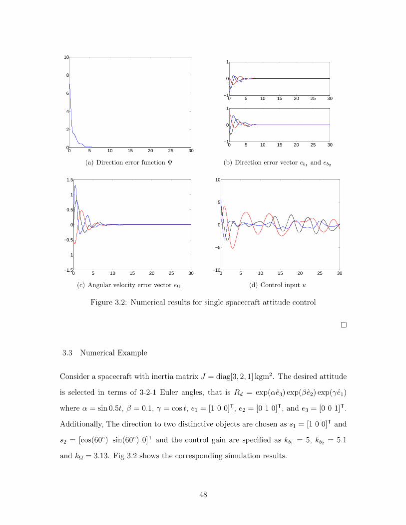
Figure 3.2: Numerical results for single spacecraft attitude control

3.3 Numerical Example

Consider a spacecraft with inertia matrix J = diag[3, 2, 1] kgm2. The desired attitude

is selected in terms of 3-2-1 Euler angles, that is Rd = exp(αe3) exp(βe2) exp(γe1)

where α = sin 0.5t, β = 0.1, γ = cos t, e1 = [1 0 0]T, e2 = [0 1 0]T, and e3 = [0 0 1]T.

Additionally, The direction to two distinctive objects are chosen as s1 = [1 0 0]T and

s2 = [cos(60) sin(60) 0]T and the control gain are specified as kb1 = 5, kb2 = 5.1

and kΩ = 3.13. Fig 3.2 shows the corresponding simulation results.

48

Chapter 4 Spacecraft Relative Attitude Formation Tracking

on SO(3) Based on Line-Of-Sight Measurements

This chapter is concerned with extending previous work to achieve the goal of this

thesis, the control of relative attitude formation among multiple spacecraft by using

LOS measurements.

As the relative control for an arbitrary number of spacecraft is quite challenging.

We start from relative attitude between two spacecrafts and show the described prop-

erties explicitly. It is generalized for relative formation control among an arbitrary

number of spacecraft.

4.1 Problem Formulation

Consider an arbitrary number n of spacecraft in formation. Each spacecraft is consid-

ered as a rigid body, and an inertial reference frame and corresponding n body-fixed

frames are defined. The attitude of each spacecraft is the orientation of its body-fixed

frame with respect to the inertial reference frame, and it is represented by a rotation

matrix in the special orthogonal group, SO(3) = R ∈ R3×3 | RTR = I, det(R) = 1.

Each spacecraft measures the LOS from itself toward the other assigned spacecraft.

A LOS observation is represented by a unit vector in the two-sphere, defined as

S2 = s ∈ R3 | ‖s‖ = 1. The nonlinear properties of S2 and SO(3) has been

addressed in Chapter 2 and Chapter 3, respectively.

49

4.1.1 Spacecraft Attitude Formation Configuration

We hereby define the configuration variables as follows, for i, j ∈ 1, . . . , n and i 6= j,

Ri(t) ∈ SO(3) the absolute attitude for the i-th spacecraft, representing the trans-

formation from the i-th body-fixed frame to the inertial reference

frame,

sij ∈ S2 the unit vector toward the j-th spacecraft from the i-th spacecraft,

represented in the inertial frame,

bij(t) ∈ S2 the LOS direction observed from the i-th spacecraft to the j-th

spacecraft, represented in the i-th body fixed frame,

Qij(t) ∈ SO(3) the relative attitude of the i-th spacecraft with respect to the j-th

spacecraft,

Qdij(t) ∈ SO(3) the desired relative attitude for Qij.

According to these definitions, the directions of the relative positions sij in the inertial

reference frame are related to the LOS observation bij in the i-th body-fixed frame as

follows:

sij = Ribij, bij = RTi sij. (4.1)

In short, bij represents the LOS observation of sij, observed from the i-th body. The

relative attitude is given by

Qij = RTj Ri, (4.2)

50

which represents the transformation of the representation of a vector from the i-th

body fixed frame to the j-th body-fixed frame. Note that

Qij = RTj Ri = (RT

i Rj)T = QT

ji. (4.3)

To assign sets of LOS that should be measured for each spacecraft, a graph (N , E)

and related sets are defined as follows.

N = 1, . . . , n the node set, hence each spacecraft is considered as a node,

E ⊂ N ×N the edge set. The relative attitude between the i-th spacecraft and

the j-th spacecraft is directly controlled if (i, j) ∈ E ,

ρ : E → N the assignment map,

A the assignment set,

Li the measurement set, the set of LOS measurements from the i-th

spacecraft,

Cij the communication set, the LOS transfered from the i-th spacecraft

to the j-the spacecraft.

The graph (N , E) represents a set of LOS that should be measured for each space-

craft. Notice that E is symmetric, specifically, (i, j) ∈ E ⇔ (j, i) ∈ E . For each pair

of spacecraft in the edge set E , another third spacecraft is assigned by the assignment

map ρ. Moreover, ρ is also a symmetric, i.e., ρ(i, j) = ρ(j, i). The definition of the

assignment set is given by

A = (i, j, k) ∈ E ×N | (i, j) ∈ E , k = ρ(i, j). (4.4)

In particular, we have the following assumptions to describe the problem clearly:

Assumption 1. The configuration of the relative positions is fixed, i.e., sij = 0 for

all i, j ∈ N with i 6= j.

51

Assumption 2. The third spacecraft assigned to each edge does not lie on the line

joining two spacecraft connected by the edge, i.e., sik × sjk , sijk 6= 0 for every

(i, j, k) ∈ A.

Assumption 3. The measurement set of the i-th spacecraft is given by

Li = bij, bik ∈ S2 | (i, j, k) ∈ A. (4.5)

Assumption 4. The communication set from the i-th spacecraft to the j-th space-

craft is given by

Cij =

bij, biρ(i,j) if (i, j) ∈ E ,

∅ otherwise.

(4.6)

Assumption 5. In the edge set, spacecraft are paired serially by daisy-chaining.

The first assumption reflects the fact that this thesis does not consider the transla-

tional dynamics of spacecraft, and we focus on the rotational attitude dynamics only.

The proposed control input does not depend on the values of sij, but its stability

analyses is based on the first assumption that sij is fixed. The second assumption is

required to determine the relative attitude between two spacecraft paired in the edge

set from the assigned LOS measurements. The third assumption states that each

spacecraft measures the LOS toward the paired spacecraft in the edge set, and the

LOS toward the third spacecraft assigned to each pair by the assignment map. The

fourth assumption implies that a spacecraft communicate only with the spacecraft

paired with itself. The last assumption is made to simplify stability analysis while

the proposed relative attitude formation control system can be extended for other

network topologies.

52

Spacecraft 4

Spacecraft 3

Spacecraft 2

Spacecraft 1

s43

s42

s34

s31

s32

s23

s21

s13

s12sij = Ribij

bij = RTi sij

Figure 4.1: Formation of four spacecrafts: the direction along the relative position ofthe i-th body from the j-th body is denoted by sij in the inertial reference frame. TheLOS observation of sij with respect the i-th body fixed frame, namely bij is obtainedfrom (4.1).

53

An example for formation of four spacecraft satisfying these assumptions are il-

lustrated at Figure 4.1, where

A = (1, 2, 3), (2, 1, 3), (2, 3, 1), (3, 2, 1), (3, 4, 2), (4, 3, 2).

The measurement sets and the communication sets can be determined by (4.5) and

(4.6) from A. For example, for the third spacecraft, we have L3 = b31, b32, b34,

C32 = b32, b31, and C34 = b34, b32.

4.1.2 Spacecraft Attitude Dynamics

Similar to (3.3) and (3.4), the equations of motion for the attitude dynamics of each

spacecraft are given by

JiΩi + Ωi × JiΩi = ui, (4.7)

Ri = RiΩi, (4.8)

where Ji ∈ R3×3 is the inertia matrix of the i-th spacecraft, and Ωi ∈ R3 and ui ∈ R3

are the angular velocity and the control moment of the i-th spacecraft, represented

with respect to its body-fixed frame, respectively. In particular, it is assumed that

the desired angular velocities are bounded by known constants.

Assumption 6. For known positive constants Bd,

‖Ωdi (t)‖ ≤ Bd,

for all t ≥ 0.

54

4.1.3 Kinematics of Relative Attitudes and Line-Of-Sight

For any i, j ∈ N , the time-derivative of the relative attitude is given, from (4.8) and

(4.2), by

Qij = −ΩjRTj Ri +RT

j RiΩi = QijΩi − ΩjQij = Qij(Ωi −QTijΩj)

∧

, QijΩij, (4.9)

where the relative angular velocity Ωij ∈ R3 of the i-th spacecraft with respect to the

j-th spacecraft is defined as

Ωij = Ωi −QTijΩj. (4.10)

From (4.1) and (4.8), the time-derivative of the LOS measurement bij is given by

bij = RTi sij = −ΩiR

Ti sij = bij × Ωi. (4.11)

Define bijk ∈ R3 where bijk , bij × bik. From (4.11) and (4.2), it can be shown that

bijk = (bij × Ωi)× bik + bij × (bik × Ωi)

= −(Ωi · bik)bij + (Ωi · bij)bik

= bijk × Ωi. (4.12)

4.2 Relative Attitude Tracking Between Two Spacecrafts

As a concrete example, we develop a control system for the relative attitude between

Spacecraft 1 and Spacecraft 2, namely Q12 = RT2R1 illustrated at Figure 4.1. The

corresponding edge set, assignment set and measurement sets used in this section are

55

given by

E = (1, 2), (2, 1), A = (1, 2, 3), (2, 1, 3), (4.13)

L1 = C12 = b12, b13, L2 = C21 = b21, b23. (4.14)

Notice that we are controlling spacecraft 1 and 2, which are considered as nodes, while

the spacecrafts 3 belongs to the assignment map. Spacecraft 3 is required because we

need an object that can be measured from spacecraft 1 and 2.

Suppose that a desired relative attitude Qd12(t) is given as a smooth function of

time. It satisfies the following kinematic equation:

Qd12 = Qd

12Ωd12, (4.15)

where Ωd12 is the desired relative angular velocity.

Our goal is to design control inputs u1, u2 in terms of the LOS measurements in

L1 ∪ L2 such that Q12 asymptotically follows Qd12, i.e., Q12(t)→ Qd

12(t) as t→∞.

4.2.1 Kinematics of Relative Attitude

It has been shown that four LOS measurements in L1 ∪L2 completely determine the

relative attitude Q12 from the following constraints [10]:

b12 = −QT12b21, (4.16)

b123

‖b123‖= −Q

T12b213

‖b213‖. (4.17)

These are derived from the fact that four unit vectors, namely, s12, s13, s21 and s23,

lie on the sides of a triangle composed of three spacecraft. In particular, the first

constraint (4.16) states that the unit vector from Spacecraft 1 to Spacecraft 2 is

exactly opposite to the unit vector from Spacecraft 2 to Spacecraft 1, i.e., s12 = −s21.

56

The second constraint (4.17) implies that the plane spanned by s12 and s13 should

be co-planar with the plane spanned by s21 and s23. These geometric constraints

are simply expressed with respect to the first body-fixed frame to obtain (4.16) and

(4.17). In consequence, the relative attitude Q12 is determined uniquely by the LOS

measurements b12, b13, b21, b23 according to (4.16) and (4.17).

We develop a relative attitude tracking control system based on these two con-

straints. More explicitly, control inputs are chosen such that two constraints are

satisfied when the relative attitude is equal to its desired value. As both constraints

are conditions on unit vectors, controller design similar to tracking control on the

two-sphere. From now on, variables related to the type of first constraint we just in-

troduced, (4.16) are denoted by the sub- or super-script α while β refers to variables

related to the second type constraint, (4.17).

The α-type configuration error function are defined as

Ψα12 =

1

2‖b21 +Qd

12b12‖2 = 1 + b21 ·Qd12b12 (4.18)

= 1 + (RT2 s21) · (Qd

12RT1 s12) = 1 + s21 ·R2Q

d12R

T1 s12. (4.19)

It is equivalent to Ψα12 = 1− cos(θα12), where θα12 is the angle between b21 and −Qdb12.

The corresponding error vectors can be defined by using the direction derivative of

Ψij, i.e., (4.19). This process is analogous to preceding work in Chapter 3, expressly,

from (3.16) to (3.18). By following the same approach, the α-type error vectors are

defined as follows:

eα12 = (Qd12

Tb21)× b12 = (Qd

21b21)× b12,

eα21 = (Qd12b12)× b21. (4.20)

57

The β-type error function are defined by

Ψβ12 = 1 +

1

a12

b213 ·Qd12b123, (4.21)

where a12 = a21 , ‖b213‖‖b123‖ ∈ R. Since ‖bijk‖ = ‖bij × bik‖ = ‖RTi sij × RT

i sik‖ =

‖sij × sik‖, the constant a12 is fixed according to Assumption 1, and it is non-zero

from Assumption 2. In particular, Ψβ12 stands for the error between Qdb123 and −b213.

Furthermore, the configuration error vectors are given as

eβ12 =1

a12

(Qd12

Tb213)× b123 =

1

a12

(Qd21b213)× b123, (4.22)

eβ21 =1

a21

(Qd12b123)× b213. (4.23)

As b12, b21 are unit vectors, and from the definition of a12, a21, we can show that the

upper bound bonds of all the error vectors, ‖eα12‖, ‖eα21‖, ‖eβ12‖, ‖e

β21‖ ≤ 1.

We also define the angular velocity errors:

eΩ1 = Ω1 − Ωd1, eΩ2 = Ω2 − Ωd

2, (4.24)

where the desired absolute angular velocities Ωd1 and Ω2

d are chosen such that

Ωd12 = Ωd

1 −Qd21Ωd

2. (4.25)

This corresponds to (4.10). Any desired absolute angular velocities satisfying (4.25)

can be chosen. For example, they can be selected as

Ω1d =1

2Ωd

12, Ω2d =1

2Ωd

21 = −Qd12Ω1d .

Using these desired angular velocities, the derivative of the desired relative attitude

58

can be rewritten as

Qd12 = Qd

12Ωd1 − Ωd

2Qd12. (4.26)

The properties of these error variables are summarized as follows.

Proposition 4.1. For positive constants kα12 6= kβ12, define

Ψ12 = kα12Ψα12 + kβ12Ψβ

12, (4.27)

e12 = kα12eα12 + kβ12e

β12, (4.28)

e21 = kα21eα21 + kβ21e

β21, (4.29)

where kα21 = kβ21, kβ21 = kβ12. The following properties hold:

(i) e12 = −Qd21e21, and ‖e12‖ = ‖e21‖.

(ii) ddt

Ψ12 = e12 · eΩ1 + e21 · eΩ2 .

(iii) ‖e12‖ ≤ (kα12 + kβ12)(‖eΩ1‖+ ‖eΩ2‖) +Bd‖e12‖,

‖e21‖ ≤ (kα12 + kβ12)(‖eΩ1‖+ ‖eΩ2‖) +Bd‖e21‖.

(iv) If Ψ12 ≤ ψ < 2minkα12, kβ12 for a constant ψ, then Ψ is quadratic with respect

to ‖e12‖, i.e., the following inequality is satisfied:

ψ12‖e12‖2 ≤ Ψ12 ≤ ψ12‖e12‖2, (4.30)

where the constants ψ12, ψ12 are given by

ψ12

=minkα12, k

β12

2max(kα12)2, (kβ12)2, (kα12 − kβ12)2+ 2(kα12 + kβ12)2

,

ψ12 =minkα12, k

β12(kα12 + kβ12)

min(kα12)2, (kβ12)2(2minkα12, kβ12 − ϕ)

.

59

Proof. Throughout this proof, we use the symbolic representation for property 1 and

2 to show that this proposition can be applied to arbitrary spacecraft i and j. From

(4.20), eαij is given by

eαij = (Qdjibji)× bij = Qd

ji(bji ×Qdijbij) = −Qd

jieαji.

Likewise, eβij = −Qdjie

βji. The symbolic form of (4.28) and (4.29) can be denoted by

eij = kαij(−Qdjie

αji) + kβij(−Qd

jieβji) = −Qd

ji(kαjie

αji + kβjie

βji) = −Qd

jieji (4.31)

where we have applied kαij = kβji and kαij = kβji. Since Qdij ∈ SO(3), any vector

multiplied by Qdij may change its direction but not the magnitude, thus ‖eij‖ = ‖eji‖.

These show (i).

From (4.19), the time-derivative of Ψαij is given by

Ψαij = sji · (RjQ

dijR

Ti sij) + sji · (RjQ

dijR

Ti sij) + sji · (RjQ

dijR

Ti sij). (4.32)

Define Ψαij = A+B where

A = sji · [RjQdij(R

Ti sij) +RjQ

dij(R

Ti )sij], (4.33)

B = sji · (RjQdijR

Ti sij). (4.34)

By applying Ri = RiΩi and sij = sji = 0, A becomes

A = sTjiRjΩjQdij(R

Ti sij) + sTjiRjQ

dij(RiΩi)

Tsij

= (RTj sji)

TΩjQdij(R

Ti sij) + (RT

j sji)TQd

ijΩTi (RT

i sij)

= bji · ΩjQdijbij − bji ·Qd

ijΩibij

= bji · [Ωj × (Qdijbij)]− (Qd

ij

Tbji) · (Ωi × bij) (4.35)

60

From the triple product expansion, x · (y × z) = y · (z × z) = z(x × y) for x, y, and

z ∈ R3

A = Ωi · [(Qdij

Tbji)× bij] + Ωj · [(Qd

ijbij)× bji] = Ωi · eαij + Ωj · eαji. (4.36)

For B, we substitute (4.26) and obtain

B = sji · (RjQdijR

Ti sij) = sTjiRj(Q

dijΩ

di − Ωd

jQdij)R

Ti sij. (4.37)

Then we apply (4.1), i.e., RTi sij = bij yield

B = (Qdij

TRTj sji)

TΩdi bij − bTjiΩd

j (Qdijbij)

= (Qdij

Tbji) · Ωd

i bij − bji · [Ωdj × (Qd

ijbij)]

= Ωdi · [bij × (Qd

ij

Tbji)]− Ωd

j · [(Qdijbij)× bji]

= −Ωdi · eαij − Ωd

j · eαji. (4.38)

Combine (4.36) with (4.38), to obtain

Ψαij = eαij · (Ωi − Ωd

i ) + eαji · (Ωj − Ωdj ) = eαij · eΩi

+ eαji · eΩj. (4.39)

Similarly, we can write

Ψβij = eβij · eΩi

+ eβji · eΩj, (4.40)

Then, substituting (4.39) and (4.40) into (4.27), (ii) is verified.

From (4.20), the time-derivative of eαij is shown as

eαij =d

dt(Qd

ij

Tbji)× bij + (Qd

ij

Tbji)× bij. (4.41)

61

First, we have

d

dt(Qd

ij

Tbji) = (Qd

ij)Tbji +Qd

ij

Tbji = (Qd

ijΩdi − Ωd

jQdij)

Tbji +Qdij

T(−Ωjbji), (4.42)

where we have applied (4.26), and (4.11). Then we can rearrange the equation as

d

dt(Qd

ij

Tbji) = −Ωd

iQdij

Tbji +Qd

ij

T(Ωd

j − Ωj)bji

= −ΩdiQ

dij

Tbji +Qd

ij

T(Ωd

j − Ωj)QdijQ

dij

Tbji. (4.43)

Apply (A.4) at the second term. Then,

d

dt(Qd

ij

Tbji) = −Ωd

iQdij

Tbji + [Qd

ij

T(Ωd

j − Ωj)]∧Qd

ij

Tbji

= −[Ωdi +Qd

ij

T(Ωj − Ωd

j )]∧Qd

ij

Tbji

= (Qdij

Tbji)× (Ωd

i +Qdij

TeΩj

). (4.44)

Next, substituting (4.44) and (4.11) into (4.41),

eαij =d

dt(QT

d bji)× bij + (QTd bji)× bij

= [(Qdij

Tbji)× (Ωd

i +Qdij

TeΩj

)]× bij + (Qdij

Tbji)× (bij × Ωi)

= −bij × [(Qdij

Tbji)× (Ωd

i +Qdij

TeΩj

)] + (Qdij

Tbji)× (bij × Ωi). (4.45)

62

By applying x× (y × z) = y(x · z)− z(x · y) for x, y, z ∈ R3, we obtain

eαij = −(Qdij

Tbji)[bij · (Ωd

i +Qdij

TeΩj

)] + (Ωdi +Qd

ij

TeΩj

)[bij · (Qdij

Tbji)]

+ bij[(Qdij

Tbji) · Ωi]− Ωi[(Q

dij

Tbji) · bij]

= −(Qdij

Tbji)[bij · (Ωd

i +Qdij

TeΩj

)] + bij[(Qdij

Tbji) · Ωi]

+ (Ωdi +Qd

ij

TeΩj− Ωi)[(Q

dij

Tbji) · bij]

= −(Qdij

Tbji)(b

Tij)(Ω

di +Qd

ij

TeΩj

) + bij[(Qdij

Tbji)

T(eΩi+ Ωd

i )]

+ [Qdij

TeΩj− (Ωi − Ωd

i )][(Qdij

Tbji) · bij], (4.46)

where we have applied Ωi = eΩi+ Ωd

i from (4.24). Then, we expand every term in

the equation.

eαij = [−(Qdij

Tbji)(b

Tij)Ω

di − (Qd

ij

Tbji)(bij)

T(Qdij

TeΩi

)] + [bij(Qdij

Tbji)

TeΩj

+ bij(Qdij

Tbji)

TΩdi ] + (Qd

ij

TeΩj− eΩi

)[(Qdij

Tbji) · bij]

= bij(Qdij

Tbji)

TΩdi − (Qd

ij

Tbji)(bij)

TΩdi − (Qd

ij

Tbji)(b

Tij)(Q

dij

TeΩj

)

+ bij(Qdij

Tbji)

TeΩi+Qd

ij

TeΩj

[(Qdij

Tbji) · bij]− eΩi

[(Qdij

Tbji) · bij]. (4.47)

Notice that we rearranged the equation such that (A.3) can be directly applied. The

yields

eαij = [(Qdij

Tbji)× bij]∧Ωd

i − (Qdij

Tbji)(bij)

T(Qdij

TeΩj

)

+ bij(Qdij

Tbji)

TeΩi+ (Qd

ij

TeΩj

)bTij(Qdij

Tbji)− eΩi

[(Qdij

Tbji)

T]bij

= [(Qdij

Tbji)× bij]× Ωd

i + (Qdij

TeΩj

)bTij(Qdij

Tbji)

− (Qdij

Tbji)(bij)

T(Qdij

TeΩj

) + bij(Qdij

Tbji)

TeΩi− eΩi

[(Qdij

Tbji)

T]bij

= eαij × Ωdi + bij × [Qd

ij

TeΩj

)× (Qdij

Tbji)] + (Qd

ij

Tbji)× (bij × eΩi

). (4.48)

63

Consequently, we can further derive the upper bound of eαij,

‖eαij‖ ≤ Bd‖eαij‖+ ‖eΩj‖+ ‖eΩi

‖. (4.49)

Following the same approach,

eβij = eβij × Ωdi + bijk × [Qd

ij

TeΩj

)× (Qdij

Tbjik)] + (Qd

ij

Tbjik)× (bijk × eΩi

), (4.50)

and

‖eβij‖ ≤ Bd‖eβij‖+ ‖eΩj‖+ ‖eΩi

‖. (4.51)

Combine (4.49), (4.51) with eij = kαijeαij + kβije

βij to obtain

‖eij‖ ≤ (kαij + kβij)(‖eΩi‖+ ‖eΩj

‖) +Bd‖eij‖, (4.52)

which shows (iii).

The procedure to show (iv) is analogous to the proof of property (iii) of Proposition

3.1. We will skip the extensive derivations and only show the important equations.

The alternative expression for Ψij is as given follows

Ψij = kαij + kβij − tr[QdijR

Ti (kαijsijs

Tij + kβij

1

‖sijk‖sijks

Tijk)Rj],

= tr[Gij(I − UTijRjQ

dijR

Ti Uij)], (4.53)

where

Kij = Kji , kαijsijsTij + kβij

1

‖sijk‖sijks

Tijk , UijGijU

Tij . (4.54)

The matrix Gij is the diagonal matrix given by Gij = diag[kαij, kβij, 0] ∈ R3, and Uij is

64

an orthonormal matrix defined as Uij = [sij,sijk‖sijk‖

,sij×sijk‖sij×sijk‖

] ∈ SO(3). Furthermore,

the derivative of Ψij with respect to Ri along the direction of δRi = Riηi correspond

to eij is expressed by

DRiΨ ·Riηi = −ηi · (RT

i KijRjQdij −Qd

ij

TRTjKijRi)

∨ = ηi · eij, (4.55)

which gives rise to an alternative expression for eij:

eij = (Qdij

TRTjKijRi −RT

i KijRjQdij)∨. (4.56)

From the Proposition 1 in [44], we have

Φij =1

2tr[Fij(I − Pij)], (4.57)

ePij =1

2(FijPij − PT

ijFij)∨, (4.58)

h6

h7 + h8

‖ePij‖2 ≤ Φij ≤h6h9

h10(h6 − ϕ)‖ePij‖2, (4.59)

where Fij = [fa, fb, fc] ∈ R3×3 is a diagonal matrix with non-negative constants fa, fb

and fc, ad P ∈ SO(3) is a rotation matrix. If Φij < ϕ < h6 for a constant ϕ, where

h6–h10 are given by

h6 = minfa + fb, fb + fc, fc + fa,

h7 = max(fa − fb)2, (fb − fc)2, (fc − fa)2,

h8 = max(fa + fb)2, (fb + fc)

2, (fc + fa)2,

h9 = maxfa + fb, fb + fc, fc + fa,

h10 = min(fa + fb)2, (fb + fc)

2, (fc + fa)2.

Compare (4.53) with (4.57), we have Fij = 2Gij and Pij = UTijRjQ

dijR

Ti Uij which

65

leads to Ψij = Φ. Furthermore (4.58) can also be updated to

ePij = (UTijRiQ

dij

Teji)

∧.

Thus, ePij = UTijRi(Q

dij)

Teji, which implies that ‖ePij‖ = ‖eji‖ = ‖eij‖ since Uij, Ri and

Qdij are all rotation matrices have unit magnitude, respectively.

Therefore, (4.59) can be rewrite as follows

h6

h7 + h8

‖eij‖2 ≤ Φij ≤h6h9

h10(h6 − ϕ)‖eij‖2. (4.60)

Then, with fa = 2kαij, fb = 2kβij, fc = 0, we denote h6h7+h8

and h6h9h10(h6−ϕ)

by ψij

and ψij,

respectively, which shows (iv).

4.2.2 Relative Attitude Tracking

Using the properties derived in the preceding section, we develop a control system to

track the given desired relative attitude as follows.

Proposition 4.2. Consider the attitude dynamics of spacecraft given by (4.7), (4.8)

for i ∈ 1, 2, with the LOS measurements specified at (4.13). A desired relative

attitude trajectory is given by (4.15). For positive constants kαij 6= kβij, kαij = kαji, k

βij =

kβji, kΩi, kΩj

, control inputs are chosen as

ui = −eij − kΩieΩi

+ Ωdi Ji(eΩi

+ Ωdi ) + JΩd

i , (4.61)

where (i, j) ∈ E . Then, the following properties hold:

(i) There are four types of equilibrium, given by the desired equilibrium (Q12,Ω12) =

(Qd12,Ω

d12), and the relative configurations represented by Qd

12 = RT2UDU

TR1

and Ω12 = Ωd12 where D ∈ diag[1,−1,−1], diag[−1, 1,−1], diag[−1,−1, 1] and

U ∈ SO(3) is the matrix composed of eigenvectors of K12 given at (4.54).

66

(ii) The desired equilibrium is almost globally exponentially stable, and a (conser-

vative) estimate to the region of attraction is given by

Ψ12(0) ≤ ψ < 2minkα12, kβ12, (4.62)∑

i=1,2

λMi‖eΩi

(0)‖2 ≤ 2(ψ −Ψ12(0)), (4.63)

where ψ is a positive constant satisfying ψ < 2 minkα12, kβ12, and λMi

denotes

the maximum eigenvalue of Ji.

(iii) The undesired equilibria are unstable.

The overall feature of this controller is in a similar manner with Proposition 3.2,

with the main difference that here we control the relative attitude between spacecraft.

The absolute attitude of each spacecraft is not required in this proposition.

Proof. From (4.7), (4.61), and rearranging, the time-derivative of JieΩiis given by

JieΩi= −(eΩi

+ Ωdi )× Ji(eΩi

+ Ωdi ) + ui − JiΩd

i , (4.64)

= (JieΩi+ JΩd

i )∧eΩi

− eij − kΩieΩi. (4.65)

The equilibrium configurations are where e12 = e21 = eΩ1 = eΩ2 = 0, which corre-

sponds to the critical points of the configuration error function given by (4.53). In

[45], it has been shown that there are four critical points:

R1Qd21R

T2 ∈ I, UD1U

T, UD2UT, UD3U

T,

where D1 = diag[1,−1,−1], D2 = diag[−1, 1,−1], D3 = diag[−1,−1, 1]. This shows

(i).

Next, we show exponential stability of the desired equilibrium. A sufficient condi-

67

tion on the initial conditions to satisfy (4.30) is obtained from the following variable:

U =1

2eΩ1 · J1eΩ1 +

1

2eΩ2 · J2eΩ2 + Ψ12.

From (4.65) and the property (ii) of Proposition 4.1, the time-derivative of U is simply

given by

U = eΩ1 · (−e12 − kΩ1eΩ1) + eΩ1 · (−e12 − kΩ1eΩ1) (4.66)

+ e12 · eΩ1 + e21 · eΩ2 (4.67)

= −kΩ1‖eΩ1‖2 − kΩ2‖eΩ2‖2 ≤ 0, (4.68)

which implies that U(t) is non-increasing. For the initial conditions satisfying (4.62),

(4.63), we have

U(0) ≤ 1

2

∑i=1,2

λMi‖eΩi

(0)‖2 + Ψ12(0) ≤ ψ.

As U(0) is non-increasing,

Ψ12(t) ≤ U(t) ≤ U(0) ≤ ψ < 2 minkα12, kβ12.

Therefore, Ψ12(t) ≤ ψ < h1 for all t ≥ 0, and the inequality (4.30) is satisfied.

Let a Lyapunov function be

V = U + c(e12 · eΩ1 + e21 · eΩ2),

for a constant c. Using (4.30), it can be shown that

∑i,j∈E

zTijM ijzij ≤ V ≤∑i,j∈E

zTijM ijzij, (4.69)

68

where zij = [‖eij‖, ‖eΩi‖] ∈ R2, and the matrices M ij,M ij ∈ R2×2 are defined as

M ij =1

2

ψij −c−c λmi

, M ij =1

2

ψij c

c λMi

, (4.70)

for (i, j) ∈ E = (1, 2), (2, 1), where it is assumed that ψij

= ψji

, ψij = ψji. From

(4.68), we obtain

V =∑i,j∈E

−kΩi‖eΩi‖2 + c(eij · eΩi

+ eij · eΩi). (4.71)

For any vector x, y ∈ R3 and square matrix Ji ∈ R3×3, we have the following proper-

ties: λmix ≤ Jix ≤ λMi

x and −x · y ≤ ‖x‖‖y‖. From (4.65) and the two properties

just mentioned, it can be shown that

eΩi· eij = J−1

i [Ji(eΩi+ Ωd

i )]∧eΩi

· eij − J−1i ‖eij‖2 − kΩi

J−1i eΩi

· eij

≤ λM−1i‖[λMi

(eΩi+ Ωd

i )]∧eΩi‖‖ei‖ − λm−1

i‖eij‖2 + kΩi

λM−1i‖eΩi‖‖eij‖,

(4.72)

where λM−1i

and λM−1i

denote the maximum and the minimum eigenvalue of the

matrix J−1i , respectively. Also, applying xy ≤ ‖x‖‖y‖ for x, y ∈ R3, λM−1

i= 1

λmiand

λm−1i

= 1λMi

gives rise to

eΩi· eij ≤

1

λmi

‖λMieΩieΩi

+ λMiΩdi eΩi‖‖eij‖ −

1

λmi

‖eij‖2 + kΩi

1

λmi

‖eΩi‖‖eij‖

≤ ‖eij‖λmi

(λmi‖eΩi‖2 + λMi

‖Ωdi ‖‖eΩi

‖)− 1

λMi

‖eij‖2 + kΩi

1

λmi

‖eΩi‖‖eij‖

≤ ‖eij‖λmi

(λMi‖eΩi‖2 + λMi

Bd‖eΩi‖)− 1

λMi

‖eij‖2 + kΩi

1

λmi

‖eΩi‖‖eij‖

=‖eij‖λmi

(‖λMi‖eΩi‖2 + λMi

Bd‖eΩi‖)− 1

λMi

‖eij‖2 + kΩi

1

λmi

‖eΩi‖‖eij‖.

(4.73)

69

From the fact that ‖eij‖ ≤ kαij + kβij, we have

eΩi· eij ≤

λMi

λmi

(kαij + kβij)‖eΩi‖2 +

λMiBd

λmi

‖eij‖‖eΩi‖ − 1

λMi

‖eij‖2 + kΩi

1

λmi

‖eΩi‖‖eij‖

=λMi

λmi

(kαij + kβij)‖eΩi‖2 +

λMiBd + kΩi

λmi

‖eij‖‖eΩi‖ − 1

λMi

‖eij‖2. (4.74)

Together with the property (iii) of Proposition 4.1, this yields the following inequality:

V ≤∑i,j∈E

−(kΩi− ckij(1 +

λMi

λmi

))‖eΩi‖2 − c

λMi

‖eij‖2 + ckij‖eΩi‖‖eΩj

‖

+c

λmi

(λiBd + kΩi

)‖eij‖‖eΩi‖, (4.75)

where λi denotes λi = λMi+ λmi

, and kij denotes kij = kαij + kβij. Expanding the

summation index, we now have

V ≤ −[kΩ1 − ck12(1 +λM1

λm1

)]‖eΩ1‖2 − c

λM1

‖e12‖2 + ck12‖eΩ1‖‖eΩ2‖

+c

λm1

(λ1Bd + kΩ1)‖e12‖‖eΩ1‖

− [kΩ2 − ck21(1 +λM2

λm2

)]‖eΩ2‖2 − c

λM2

‖e21‖2 + ck21‖eΩ2‖‖eΩ1‖

+c

λm2

(λ2Bd + kΩ2)‖e21‖‖eΩ2‖, (4.76)

then, we can rearrange the equation to obtain

V ≤ −[12kΩ1 − ck12(1 +

λM1

λm1

)]‖eΩ1‖2 +c

λM1

‖e12‖2

− c

λm1

(λ1Bd + kΩ1)‖e12‖‖eΩ1‖ − [

1

2kΩ2 − ck21(1 +

λM2

λm2

)]‖eΩ2‖2

+c

λM2

‖e21‖2 − c

λm2

(λ2Bd + kΩ2)‖e21‖‖eΩ2‖

− 1

2kΩ1‖eΩ1‖2 +

1

2kΩ2‖eΩ2‖2 − 2ck12‖eΩ1‖‖eΩ2‖, (4.77)

70

which can be rewritten as the following matrix form:

V ≤ −zT12W12z12 − zT21W21z21 − ζT12Y12ζ12, (4.78)

where ζ12 = [‖eΩ1‖, ‖eΩ2‖]T ∈ R2 and the matrices W12,W21, Y12 ∈ R2×2 are given by

Wij =1

2

2 cλMi

− cλmi

(λiBd + kΩi

)

− cλmi

(λiBd + kΩi

) kΩi− 2ckij(1 +

λMi

λmi)

, (4.79)

Y12 =1

2

kΩ1 −2ck12

−2ck12 kΩ2

. (4.80)

for (i, j) ∈ E . Thus, we choose the constant c such that

c < min√ψ

12λm1 ,

√ψ

21λm2 ,

√ψ12λM1 ,

√ψ21λM2 ,

√kΩ1kΩ2

2k12

,

2kΩ1λ2m1

4k12λm1(λ1) + λM1(Bdλ1 + kΩ1)

2,

2kΩ2λ2m2

4k21λm2(λ2) + λM2(Bdλ2 + kΩ2)

2

(4.81)

The first four conditions come from (4.69) and (4.70) to ensure the Lyapunov can-

didate to be a positive-definite function. The last three terms come from (4.79) and

(4.80). Furthermore, it is chosen such that the time-derivative of the Lyapunov can-

didate is negative-definite. Therefore, the desired equilibrium is exponentially stable.

Next, we show (iii). At the first type of undesired equilibria given by R1Qd21R

T2 =

UD1UT and eΩ1 = eΩ2 = 0, the value of the Lyapunov function becomes V = 2kβ12.

Define

W = 2kβ12 − V .

71

Then, W = 0 at the undesired equilibrium, and we have

−∑

(i,j)∈E

λMi

2‖eΩi‖2 + c‖eij‖‖eΩi

‖+ (2kβ12 −Ψ) ≤ W .

Due to the continuity of Ψ, we can choose R1 and R2 arbitrary close to the undesired

equilibrium such that (2kβ2 − Ψ) > 0. Therefore, if ‖eΩi‖ is sufficiently small, we

obtain W > 0. Therefore, at any arbitrarily small neighborhood of the undesired

equilibrium, there exists a set in which W > 0, and we have W = −V > 0 from

(4.78). Therefore, the undesired equilibrium is unstable [43, Theorem 4.3]. The

instability of other types of equilibrium can be shown similarly. This shows (iii).

The region of attraction to the desired equilibrium excludes the union of stable

manifolds to the unstable equilibria. But, the union of stable manifolds has less

dimension than the tangent bundle of the configuration manifold. Therefore, the

measure of the stable manifolds to the unstable equilibria is zero. This implies the

desired equilibrium is almost globally exponentially stable [14], which shows (ii).

The result we presented in this section can be considered as a generalization

of [10] with time-varying desired relative attitude tracking commands and stronger

exponential stability.

4.3 Relative Attitude Formation Tracking

The ultimate goal in this thesis is relative attitude formation control between n space-

craft. The key idea of relative attitude control is illustrated in the previous section

with two spacecraft, and we generate it into an arbitrary number of spacecraft in this

section.

72

4.3.1 Relative Attitude Tracking Between Three Spacecrafts

We first consider relative attitude formation tracking between three spacecraft, given

by Spacecraft 1, 2, and 3, illustrated at Figure 4.1. The corresponding edge set and

the assignment set used in this subsection are given by

E = (1, 2), (2, 1), (2, 3), (3, 2), (4.82)

A = (1, 2, 3), (2, 1, 3), (2, 3, 1), (3, 2, 1). (4.83)

For given relative attitude commands, Qd12(t), Qd

23(t), the goal is to design control

inputs such that Q12(t)→ Qd12(t) and Q23(t)→ Qd

23(t) as t→∞.

The definition of error variables and their properties developed in the previous

section for two spacecraft are readily generalized to any (i, j, k) ∈ A in this section.

For example, the kinematic equation for the desired relative attitude Qd23 is obtained

from (4.15) as

Qd23 = Qd

23Ωd23, (4.84)

where Ωd23 is the desired relative angular velocity. Other configuration error functions

and error vectors between Spacecraft 2 and Spacecraft 3 are defined similarly.

The desired absolute angular velocities for each spacecraft, namely Ωd1, Ωd

2, and

Ωd3 should be properly defined. For the given Ωd

12, Ωd23, they can be arbitrarily chosen

such that

Ωd12(t) = Ωd

1(t)−Qd21(t)Ωd

2(t), (4.85)

Ωd23(t) = Ωd

2(t)−Qd32(t)Ωd

3(t). (4.86)

For example, they can be chosen as Ωd1 = Ωd

12, Ωd2 = 0, Ωd

3 = −Qd23Ωd

23. Assumption 6

73

is considered to be satisfied such that each of the desired angular velocity is bounded

by a known constant Bd.

Proposition 4.3. Consider the attitude dynamics of spacecraft given by (4.7), (4.8)

for i ∈ 1, 2, 3, with the LOS measurements specified at (4.83). Desired relative

attitudes are given by Qd12(t), Qd

23(t). For positive constants kαij, kβij, kΩi

with kαij 6= kβij,

kαij = kαji, kβij = kβji for (i, j) ∈ E ,

u1 = −e12 − kΩ1eΩ1 + Ωd1J1(eΩ1 + Ωd

1) + JΩd1, (4.87)

u2 = −1

2(e21 + e23)− kΩ2eΩ2 + Ωd

2J2(eΩ2 + Ωd2) + JΩd

2, (4.88)

u3 = −e32 − kΩ3eΩ3 + Ωd3J3(eΩ3 + Ωd

3) + JΩd3, (4.89)

Then, the desired relative attitude configuration is almost globally exponentially sta-

ble, and a (conservative) estimate to the region of attraction is given by

Ψ12(0) + Ψ23(0) ≤ ψ < 2 minkα12, kβ12, k

α23, k

β23, (4.90)

λM1‖eΩ1(0)‖2 + 2λM2‖eΩ2(0)‖2 + λM3‖eΩ3(0)‖2 ≤ 2(ψ −Ψ12(0)−Ψ23(0)), (4.91)

where ψ is a positive constant satisfying ψ < 2 minkα12, kβ12, k

α23, k

β23.

Proof. The time-derivative of J1e1 and J3e3 are given by (4.65), and the time-derivative

of J2e2 is given by

J2eΩ2 = (J2eΩ2 + JΩd2)∧eΩ2 −

1

2(e21 + e23)− kΩ2eΩ2 . (4.92)

Define

U =1

2eΩ1 · J1eΩ1 + eΩ2 · J2eΩ2 +

1

2eΩ3 · J3eΩ3 + Ψ12 + Ψ23. (4.93)

74

From (4.65), (4.92), we have

U = −kΩ1‖eΩ1‖2 − 2kΩ2‖eΩ2‖2 − kΩ3‖eΩ3‖2, (4.94)

which implies that U(t) is non-increasing. For the initial conditions satisfying (4.90)

and (4.91), we have U(0) ≤ ψ. Therefore,

Ψ12(t) + Ψ23(t) ≤ U(t) ≤ U(0) ≤ ψ < 2 minkα12, kβ12, k

α23, k

β23. (4.95)

Therefore, the inequality (4.30) holds for both of Ψ12 and Ψ23.

Let a Lyapunov function be

V = U + ceΩ1 · e12 + ceΩ2 · (e21 + e23) + ceΩ3 · e32. (4.96)

From (4.30), we can show that this Lyapunov function satisfies the inequality given

by (4.69), that is,

V ≤ zT12M12z12 + zT21M21z21 + zT23M23z23 + zT32M32z32, (4.97)

V ≥ zT12M12z12 + zT21M21z21 + zT23M23z23 + zT32M32z32. (4.98)

where the matrices M ij and M ij are welled defined by (4.70). Moreover, the time-

derive of Lyapunov function (4.96) is similar to (4.71). We will expand V term by

term in the coming paragraph so the the sequence of idea will be clear.

For (i, j) ∈ (1, 2), (3, 2), the upper bound of eΩi· eij is given by (4.74). Alter-

natively, from (4.92), with the similar procedure in (4.72) through (4.74), the upper

75

bound of eΩ2 · (e21 + e23) is given by

eΩ2 · (e21 + e23) ≤ λM2

λm2

(k21 + k23)‖eΩ2‖2 +λM2B

d + kΩ2

λm2

‖e21 + e23‖‖eΩ2‖

− 1

2λM2

‖e21 + e23‖2. (4.99)

The upper bounds of ‖e32‖ and ‖e12‖ are given by the property (iii) of Proposition

4.1. Additionally, using (4.52), we can show that

‖e21 + e23‖ ≤ (k21 + k23)(‖eΩ1‖+ 2‖eΩ2‖+ ‖eΩ3‖) +Bd‖e21 + e23‖. (4.100)

Applying these bounds to the expression of V and rearranging, we obtain

V ≤ −[kΩ1 − ck12(1 +λM1

λm1

)]‖eΩ1‖2 − c

λM1

‖e12‖2 + ck12‖eΩ1‖‖eΩ2‖

− [kΩ3 − ck32(1 +λM3

λm3

)]‖eΩ3‖2 − c

λM3

‖e32‖2 + ck32‖eΩ3‖‖eΩ2‖

+c

λm1

(λ1Bd + kΩ1)‖e12‖‖eΩ1‖+

c

λm3

(λ3Bd + kΩ3)‖e32‖‖eΩ3‖

− [kΩ2 − ck213(2 +λM2

λm2

)]‖eΩ2‖2 +c

λm2

(λ2Bd + kΩ2)‖e21 + e23‖‖eΩ2‖

− c

2λM2

‖e21 + e23‖2 + ck213‖eΩ1‖‖eΩ2‖+ ck213‖eΩ2‖‖eΩ3‖, (4.101)

76

This can be rearranged as

V ≤ − c

λM1

‖e12‖2 − c

λm1

(λ1Bd + kΩ1)‖e12‖‖eΩ1‖+ [

1

2kΩ1 − ck12(1 +

λM1

λm1

)]‖eΩ1‖2

− c

λM3

‖e32‖2 − c

λm3

(λ3Bd + kΩ3)‖e32‖‖eΩ3‖+ [

1

2kΩ3 − ck32(1 +

λM3

λm3

)]‖eΩ3‖2

− c

2λM2

‖e21 + e23‖2 − c

λm2

(λ2Bd + kΩ2)‖e21 + e23‖‖eΩ2‖

+ [1

2kΩ2 − ck213(2 +

λM2

λm2

)]‖eΩ2‖2

− 1

2kΩ1‖eΩ1‖2 +

1

4kΩ2‖eΩ2‖2 − c(2k21 + k23)‖eΩ1‖‖eΩ2‖

− 1

4kΩ2‖eΩ2‖2 +

1

2kΩ3‖eΩ3‖2 − c(k21 + 2k23)‖eΩ2‖‖eΩ3‖. (4.102)

The corresponding matrix form is

V ≤ −zT12W12z12 − zT213W213z213 − zT32W32z32 − ζT21Z21ζ21 − ζT23Z23ζ23, (4.103)

where the matrixW12,W23 ∈ R2×2 are given as (4.79), and z213 = [‖e21+e23‖, ‖eΩ2‖]T ∈

R2. The matrices W213, Z21, Z23 ∈ R2×2 are defined as

W213 =1

2

cλM2

− cλm2

(λ2Bd + kΩ2)

− cλm2

(λ2Bd + kΩ2) kΩ2 − 2ck213(2 +

λM2

λm2)

, (4.104)

Z21 =1

2

12kΩ2 −c(2k21 + k23)

−c(2k21 + k23) kΩ1

, (4.105)

Z23 =1

2

12kΩ2 −c(k21 + 2k23)

−c(k21 + 2k23) kΩ3

, (4.106)

where k213 = k12 + k23. It can be shown that all of matrices at (4.97), (4.98) and

(4.103) are positive definite if the constant c is sufficient small. In particular, the way

to find the maximum value of c is in a similar manner with the proof of Proposition

77

2.2 and with (4.81) as well. Therefore, we now can write

V ≤ −λm(W12)(‖e12‖2 + ‖eΩ1‖2)− λm(W213)(‖e21 + e23‖2 + ‖eΩ2‖2)

− λm(W32)(‖e31‖2 + ‖eΩ3‖2)

≤ −λm(W12)

1

2(‖e12‖2 + ‖e21‖2) + ‖eΩ1‖2

− λm(W213)‖eΩ2‖2

− λm(W32)

1

2(‖e32‖2 + ‖e23‖2) + ‖eΩ3‖2

, (4.107)

where λm(·) denotes the minimum eigenvalue of a matrix, and we use the fact that

‖e12‖ = ‖e21‖, ‖e23‖ = ‖e32‖. Therefore, the desired equilibrium is exponentially

stable.

To show almost exponential stability, it is required that the fifteen types of the

undesired equilibria, corresponding to the critical points of Ψ12 and Ψ23, are unstable.

This is similar to the proof of the property (iii) of Proposition 4.2, and it is omitted.

4.3.2 Relative Attitude Formation Tracking Between n Spacecrafts

Consider a formation of n spacecraft, i.e., N = 1, . . . , n. According to Assumption

5, spacecraft are paired serially in the edge set. For convenience, it is assumed that

spacecraft are numbered such that the edge set is given by

E = (1, 2), (2, 3), . . . , (n− 1, n), (2, 1), (3, 2), . . . , (n, n− 1). (4.108)

The assignment set is given by (4.4) for an arbitrary assignment map satisfying As-

sumption 2. The desired relative attitudes Qdij for (i, j) ∈ E are prescribed. Also,

recall that the definition of error variables and their properties developed in the

Proposition 4.1 of Section 4.2 are ready generalized to any (i, j, k) ∈ A, and these

78

generalized variables become

eij = −Qdjieji, ‖eij‖ = ‖eji‖, (4.109)

Ψij = eij · eΩi+ eji · eΩj

, (4.110)

‖eij‖ ≤ (kαij + kβij)(‖eΩi‖+ ‖eΩj

‖) +Bd‖eij‖, (4.111)

ψij‖eij‖2 ≤ Ψij ≤ ψij‖eij‖2 (4.112)

where ψij

and ψij are positive constants can be determined, the way to find out these

two constants are addressed in the proof section of Proposition 4.1. Moreover, the

desired absolute angular velocities Ωdi for i ∈ N are chosen such that

Ωdij(t) = Ωd

i (t)−Qdji(t)Ω

dj (t) for (i, j) ∈ E . (4.113)

Proposition 4.4. Consider the attitude dynamics of spacecraft given by (4.7), (4.8)

for i ∈ 1, . . . , n, with the LOS measurements specified by (4.108) and (4.4). Desired

relative attitudes are given by Qdij(t) for (i, j) ∈ E . For positive constants kαij, k

βij, kΩi

with kαij 6= kβij, kαij = kαji, k

βij = kβji, and p ∈ 2, . . . , n − 1, the control inputs are

chosen as

u1 = −e12 − kΩ1eΩ1 + Ωd1J1(eΩ1 + Ωd

1) + J1Ωd1, (4.114)

up = −1

2(ep,p−1 + ep,p+1)− kΩpeΩp + Ωd

pJp(eΩp + Ωdp) + JpΩ

dp, (4.115)

un = −en,n−1 − kΩneΩn + ΩdnJn(eΩn + Ωd

n) + JnΩdn. (4.116)

Next, the desired relative attitude configuration is almost globally exponentially sta-

79

ble, and a (conservative) estimate to the region of attraction is given by

n−1∑i=1

Ψi,i+1(0) ≤ ψ < 2 min1≤i≤n−1

kαi,i+1, kβi,i+1, (4.117)

λM1‖eΩ1(0)‖2 + 2n−1∑i=2

λMi‖eΩi

(0)‖2 + λMn‖eΩn(0)‖2 ≤ 2(ψ −n−1∑i=1

Ψi,i+1(0)), (4.118)

where ψ is a positive constant satisfying ψ < 2 min1≤i≤n−1kαi,i+1, kβi,i+1.

Proof. The proof of this proposition has been carried out by the proof of Proposition

of 4.3 with tedious extension, which is also very similar to the proof of Proposition

4.2. Here we still summarize the essential equations to show the framework.

The time-derivative of J1e1 and Jnen are specified as follows, which is consistent

with (4.65)

J1(eΩ1) = (J1eΩ1 + J1Ωd1)∧eΩ1 − e12 − kΩ1eΩ1 , (4.119)

Jn(eΩn) = (JneΩn + JnΩdn)∧eΩn − en,n−1 − kΩneΩn , (4.120)

while the time-derivative of Jp, for p ∈ 2, . . . , n− 1 is

Jp(eΩp) = (JpeΩp + JpΩpd)∧eΩp −1

2(ep,p−1 + ep,p+1)− kΩpeΩp . (4.121)

Define U = Ue + UΨ where

Ue =1

2eΩ1 · J1eΩ1 +

1

2eΩn · JneΩn +

n−1∑i=2

eΩi· JieΩi

, (4.122)

UΨ =n−1∑i=1

Ψi,i+1. (4.123)

In view of (4.110) and (4.119) through (4.121), the differentiation of U with respect

80

to time is

U = Ue + UΨ = −kΩ1‖eΩ1‖2 − kΩn‖eΩn‖2 − 2n−1∑i=2

kΩi‖eΩi‖2, (4.124)

which shows U is non-decreasing. Then, the Lyapunov candidate is in the form

V = U + ceΩ1 · e12 + ceΩn · en,n−1 + c

n−1∑i=2

eΩi· (ei,i−1 + ei,i+1). (4.125)

where c is a constant which will be determined later. From (4.112), it is straightfor-

ward to show that the Lyapunov function satisfies the inequality given by (4.69).

Furthermore, for (i, j) ∈ (1, 2), (n, n− 1) the upper bound of eΩi· eij is given by

(4.74), We rewrite as follows:

eΩ1 · e12 =λM1

λm1

(kα12 + kβ12)‖eΩ1‖2 +λM1B

d + kΩ1

λm1

‖e12‖‖eΩ1‖ −1

λM1

‖e12‖2, (4.126)

and

eΩn · en,n−1 =λMn

λmn

(kαn,n−1 + kβn,n−1)‖eΩn‖2 +λMnB

d + kΩn

λmn

‖en,n−1‖‖eΩn‖

− 1

λMn

‖en,n−1‖2, (4.127)

while the rest term of eΩi· eij are given by

eΩi· (ei,i−1 + ei,i+1) ≤ λMi

λmi

(ki,i−1 + ki,i+1)‖eΩi‖2 +

λMiBd + kΩi

λmi

‖ei,i−1 + ei,i+1‖‖eΩi‖

− 1

2λMi

‖ei,i−1 + ei,i+1‖2. (4.128)

The summation of (4.124) and (4.126) through (4.128) is the time-derive of (4.125).

81

S1

S2

S3

S4

S5

S6

S7

Figure 4.2: Relative attitude formation tracking for 7 spacecraft: the lines-of-sightmeasured by each spacecraft are denoted by arrows, and the dotted line between twospacecraft implies that they are paired at the edge set.

And it can be rearranged to the matrix form

V ≤ −zT12W12z12 − zTn,n−1Wn,n−1zn,n−1 −n−1∑i=2

zTi,i−1,i+1Wi,i−1,i+1zi,i−1,i+1

−n−1∑i=1

ζTi,i+1Zi,i+1ζi,i+1, (4.129)

where zi,i−1,i+1 = [‖ei,i−1 + ei,i+1‖, ‖eΩi‖]T ∈ R2 and ζi,i+1 = [‖eΩi

‖, ‖eΩi+1‖]T. With

analogous process from (4.79) through (4.81), it can be shown that if the constant

c is sufficiently small, all the M , M , W , and Z matrices is positive definite. This

directly implies that the Lyapunov function V is positive definite and decrescent and

its time-derivative V is negative definite. Thus we conclude the exponential stability

of the desired equilibrium.

82

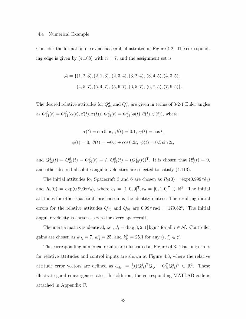
4.4 Numerical Example

Consider the formation of seven spacecraft illustrated at Figure 4.2. The correspond-

ing edge is given by (4.108) with n = 7, and the assignment set is

A = (1, 2, 3), (2, 1, 3), (2, 3, 4), (3, 2, 4), (3, 4, 5), (4, 3, 5),

(4, 5, 7), (5, 4, 7), (5, 6, 7), (6, 5, 7), (6, 7, 5), (7, 6, 5).

The desired relative attitudes for Qd34 and Qd

45 are given in terms of 3-2-1 Euler angles

as Qd34(t) = Qd

34(α(t), β(t), γ(t)), Qd45(t) = Qd

45(φ(t), θ(t), ψ(t)), where

α(t) = sin 0.5t, β(t) = 0.1, γ(t) = cos t,

φ(t) = 0, θ(t) = −0.1 + cos 0.2t, ψ(t) = 0.5 sin 2t,

and Qd12(t) = Qd

23(t) = Qd56(t) = I, Qd

67(t) = (Qd45(t))T. It is chosen that Ωd

4(t) = 0,

and other desired absolute angular velocities are selected to satisfy (4.113).

The initial attitudes for Spacecraft 3 and 6 are chosen as R3(0) = exp(0.999πe1)

and R6(0) = exp(0.990πe2), where e1 = [1, 0, 0]T, e2 = [0, 1, 0]T ∈ R3. The initial

attitudes for other spacecraft are chosen as the identity matrix. The resulting initial

errors for the relative attitudes Q23 and Q67 are 0.99π rad = 179.82. The initial

angular velocity is chosen as zero for every spacecraft.

The inertia matrix is identical, i.e., Ji = diag[3, 2, 1] kgm2 for all i ∈ N . Controller

gains are chosen as kΩi= 7, kαij = 25, and kβij = 25.1 for any (i, j) ∈ E .

The corresponding numerical results are illustrated at Figures 4.3. Tracking errors

for relative attitudes and control inputs are shown at Figure 4.3, where the relative

attitude error vectors are defined as eQij= 1

2((Qd

ij)TQij − QT

ijQdij)∨ ∈ R3. These

illustrate good convergence rates. In addition, the corresponding MATLAB code is

attached in Appendix C.

83

0 5 10 15 200

10

20

30

40

50

60

70

80

(a) Relative attitude error functionsΨ12,Ψ23, . . . ,Ψ67

0 5 10 15 20−1

0

1

0 5 10 15 20−1

0

1

0 5 10 15 20−1

0

1

(b) Relative attitude error vectorseQ12 , eQ23 , . . . , eQ67

0 5 10 15 20−5

0

5

0 5 10 15 20−2

0

2

0 5 10 15 20−1

0

1

(c) Relative angular velocity error eΩ1, . . . , eΩ7

0 5 10 15 20−20

0

20

0 5 10 15 20−50

0

50

0 5 10 15 20−10

0

10

(d) Control moments u1, . . . , u7

Figure 4.3: Numerical results for seven spacecrafts in formation (blue, green, red,cyan, magenta, and black in ascending order)

84

Chapter 5 Conclusions

5.1 Concluding Remarks

The current relative attitude control system is unique from the aspect that control

inputs are directly expressed in terms of LOS measurements such that determining the

full absolute attitude of spacecraft in formation is not required. Relative attitude are

directly controlled, and it leads to higher accuracy and a relatively low-cost compare

to other attitude determining sensors. Furthermore, the tracking command is allowed

to be continuous function of time that gives the flexibility of the formation between

each spacecrafts.

Developing attitude control system on SO(3) avoids complexities of using parame-

terization method such as Euler angle and quaternions. And even more remarkably, it

avoids the singularities and ambiguities that occur in parameterization. Additionally,

using unit vectors on S2 to express LOS measurements is a simpler way to denote

directions of spherical pendulum. This feature is more significant where there are

multiple spacecraft in the system. Furthermore, the presented stability properties are

valid globally fro all possible attitude configurations.

The relative attitude controller on SO(3) and PD controller on S2 provide almost

global exponential stability which is stronger than asymptotic stability offered by

typical Lyapunov-based tracking controller. By definition, asymptotic stability im-

plies attractivity only, i.e., the solution in the region of attraction will converge to

equilibrium as time goes to infinity even though the rate of converge may be very

85

slow. Exponential stability offer a much higher rate of convergence [43]. The PID

controller on S2 does not have exponential stability since the error of integrator does

not converge to zero, but it successfully remove the effect of fixed perturbation in the

control system, in other words, the controlled system can still perform well even poor

estimation of angular velocity is acquired.

5.2 Future Work

Vision-based spacecraft formation control on SE(3) This thesis explores rel-

ative attitude control with LOS measurements, however, the full formation includes

not only relative attitude (rotation), but also relative positions (translation). It is

possible to extend the vision-based control scheme presented in this thesis to full

formation control. Specifically, previous work have shown that the dynamics of a

spacecraft can globally expressed in the special Euclidean group, SE(3) [46], which is

the semi-direct product of R3 and SO(3). Thus, using vision-based control on SE(3)

for both rotational and translational motion is one of future directions.

Robust Spacecraft formation control The proposed relative attitude formation

control system is actually a nonlinear PD controller. As the configuration error vec-

tor, eij, represents the proportional term and the angular velocity error vector ,eΩi,

corresponds to the derivative term. Based on the unique nonlinear PID controller on

S2 proposed in Chapter 2, it is reasonable to suggest that adding the integral term to

the attitude control system of multiple spacecraft in the future to accomplish higher

level of performance.

Spacecraft formation control with bounded inputs Throughout this thesis,

we do not consider constraints of the control input, however, magnitude of control

input may be constrained because the power source in not unlimited in the real

86

world. Thus, we may use saturation functions to generate bounded control inputs as

a solution [47]. This will significantly increase practicability of the controller.

87

Bibliography

[1] D. P. Scharf, F. Y. Hadaegh, and S. R. Ploen, “A survey of spacecraft formationflying guidance and control. Part II: control,” in America Control Conference,vol. 4, 2004, pp. 2976–2985.

[2] O. P. Lay, G. H. Blackwood, S. Dubovitsky, P. W. Gorham, and R. P. Linfield,“Design of the ST 3 formation flying interferometer,” in Working on the Fringe:Optical and IR Interferometry from Ground and Space ASP Conference Series,vol. 194, 1999.

[3] E. S. Agency, “Darwin,” October 2009. [Online]. Available: http://www.esa.int/esaSC/120382 index 0 m.html

[4] M. L. Mitchell, “CDGPS-based relative navigation for multiple spacecraft,”Ph.D. dissertation, Massachusetts Institute of Technology, 2004.

[5] F. H. Bauer, K. Hartman, J. P. How, J. Bristow, D. Weidow, and F. Busse,“Enabling spacecraft formation flying through spaceborne GPS and enhancedautomation technologies,” in ION-GPS Conference, 1999, pp. 167–172.

[6] A. Khosravian and M. Namvarn, “Rigid body attitude control using a single vec-tor measurement and gyro,” IEEE Transactions on Automatic Control, vol. 57,no. 5, pp. 1273–1279, 2012.

[7] G. G. Scandaroli, P. Morlin, and G. Silveira, “A nonlinear observer approachfor concurrent estimation of pose, IMU bias and camera-to-IMU rotation,” inIEEE/RSJ International Conference on Intelligent Robots and systems, 2011,pp. 3335–33 341.

[8] G. N. DeSouza and A. C. Kak, “Vision for mobile robot navigation: a survey,”IEEE Transactions on Pattern Analysis and Machine Intelligence, vol. 24, no. 2,pp. 237–267, 2002.

[9] J. A. Guerrero and R. Lozano, Flight Formation Control. Hoboken: John Wiley& Sons, 2012.

[10] T. Lee, “Relative attitude control of two spacecraft on SO(3) using line-of-sightobservations,” in America Control Conference, 2012, pp. 167–172.

88

[11] M. D. Shuster, “A survey of attitude representations,” The Journal of Astronau-tical Sciences, vol. 41, no. 4, pp. 439–517, 1993.

[12] B. Zhang and S. Song, “Robust attitude coordination control of formation flyingspacecraft under control input saturation,” International Journal of InnovativeComputing, Information and Control, vol. 7, no. 7, pp. 4223–4235, 2011.

[13] A. K. Bondhus, K. Y. Pettersen, and J. T. Gravdahl, “Leader/follower syn-chronization of satellite attitude without angular velocity measurements,” inIEEE Conference on Decision and Control, and the European Control Confer-ence, 2005, pp. 7270–7277.

[14] N. Chaturvedi, A. Sanyal, and N. McClamroch, “Rigid-body attitude control,”IEEE Control Systems Magazine, vol. 31, no. 3, pp. 30–51, 2011.

[15] O. O. Gutirrez, C. A. Ibez, and H. Sossa, “Stabilization of the inverted sphericalpendulum via Lyapunov approach,” Asian Journal of Control, vol. 11, no. 6, pp.587–594, 2009.

[16] K. Furuta, “Control of pendulum: from super mechano-system to human adap-tive mechatronics,” in Proceedings of the 42nd IEEE onference on Decision andControl, vol. 2, 2003, pp. 1498–1507.

[17] A. Shiriaev1, A. Pogromsky, H. Ludvigsen, and O. Egeland, “On global proper-ties of passivity-based control of an inverted pendulum,” International Journalof Robust and Nonlinear Control, pp. 283–200, 2000.

[18] T. Lee, M. Leok, and N. H. McClamroch, “Lagrangian mechanics and variationalintegrators on two-spheres,” International Journal for Numerical Methods inEngineering, vol. 79, no. 9, pp. 1147–1174, 2009.

[19] J. Shen, A. K. Sanyal, N. A. Chaturvedi, D. Bernstein, and H. McClamroch,“Dynamics and control of a 3D rigid pendulum,” in IEEE Conference on Decisionand Control, vol. 1, 2004, pp. 323–328.

[20] N. A. Chaturvedi, F. Bacconi, A. K. Sanyal, D. Bernstein, and N. H. McClam-roch, “Stabilization of a 3D rigid pendulum,” in America Control Conference,vol. 5, 2005, pp. 3030–3035.

[21] A. D. Anderson, J. I. Sellers, and Y. Hashida, “Attitude determination andcontrol system simulation and analysis for low-cost micro-satellites,” in AmericaControl Conference, vol. 5, 2004, pp. 2935–3949.

[22] F. Lizarralde and J. T. Wen, “Attitude control without angular velocity measure-ment: a passivity approach,” IEEE Transactions on Automatic Control, vol. 41,no. 3, pp. 468–472, 1996.

89

[23] C. G. Mayhew, R. G. Sanfelice, and A. R. Teel, “Neural network-based dis-tributed attitude coordination control for spacecraft formation flying with in-put saturation,” IEEE Transactions on Neural Networks and Learning Systems,vol. 23, no. 7, pp. 1155–1162, 2012.

[24] ——, “Quaternion-based hybrid control for robust global attitude tracking,”IEEE Transactions on Automatic Control, vol. 56, no. 11, pp. 2555–2566, 2011.

[25] S. P. Bhat and D. S. Bernstein, “A topological obstruction to continuous globalstabilization of rotational motion and the unwinding phenomenon,” Systems andControl Letters, vol. 39, no. 1, pp. 63–70, 2000.

[26] T. Lee, “Geometric tracking control of the attitude dynamics of a rigid body onSO(3),” in America Control Conference, 2011, pp. 1200–12 055.

[27] T. Lee, M. Leok, and N. H. McClamroch, “Stable manifolds of saddle equilibriafor pendulum dynamics on S2 and SO(3),” in Decision and Control and EuropeanControl Conference, 2011, pp. 3915–3921.

[28] S. Bertrand, T. Hamel, H. Piet-Lahanier, and R. Mahony, “Attitude trackingof rigid bodies on the special orthogonal group with bounded partial state feed-back,” in IEEE Conference on Decision and Control Conference, 2009, pp. 2972–2977.

[29] R. Mahony, T. Hamel, and J. Pflimlin, “Nonlinear complementary filters on thespecial orthogonal group,” IEEE Transactions on Automatic Control, vol. 53,no. 5, pp. 1200–1211, 2008.

[30] J. A. Fax and R. M. Murray, “Information flow and cooperative control of vehicleformations,” IEEE Transactions on Automatic Control, vol. 49, no. 9, pp. 1465–1476, 2004.

[31] A. Jadbabaie, J. Lin, and A. S. Morse, “Coordination of groups of mobile au-tonomous agents using nearest neighbor rules,” IEEE Transactions on AutomaticControl, vol. 48, no. 6, pp. 2953–2958, 2003.

[32] W. Kang and H.-H. Yeh, “Co-ordinated attitude control of multi-satellite sys-tems,” International Journal of Robust and Nonlinear Control, vol. 12, pp. 185–205, 2002.

[33] T. Balch and R. C. Arkin, “Behavior-based formation control for multirobotteams,” IEEE Transactions on Robotics Automation, vol. 14, no. 6, pp. 926–939,1998.

[34] R. W. Beard, J. Lawton, and F. Y. Hadaegh, “A coordination architecture forspacecraft formation control,” IEEE Transactions on Control Systems and Tech-nology, vol. 9, no. 6, pp. 777–790, 2001.

90

[35] W. Ren and R. Beard, “Formation feedback control for multiple spacecraft viavirtual structures,” IEE Proceedings-Control Theory and Applications, vol. 151,no. 3, pp. 357–368, 2004.

[36] W. Ren and R. W. Beard, “Virtual structure based spacecraft formation controlwith formation feedback,” in AIAA Guidance, Navigation, and Control Confer-ence and Exhibit, 2002.

[37] Z.-H. Zhou, J. Yuan, W.-X. Zhang, and J.-P. Zhao, “Virtual-leader-followerstructure and finite-time controller based cooperative control of multiple au-tonomous underwater vehicles,” in IEEE Control and Decision Conference, 2012,pp. 3670–3675.

[38] P. Corke, Robotics, Vision and Control: Fundamental Algorithms in MATLAB.Berlin: Springer-Verlag, 2011.

[39] Y. Wang, W. Yan, and W. Yan, “A leader-follower formation control strategyfor auvs based on line-of-sight guidance,” in IEEE International Conference onMechatronics and Automation, 2009, pp. 4863–4867.

[40] M. S. Andrle, J. L. Crassidis, R. Linares, Y. Cheng, and B. Hyun, “Deter-ministic relative attitude determination of three-vehicle formations,” Journal ofGuidance, Control, and Dynamics, vol. 32, no. 4, pp. 1077–1088, 2009.

[41] R. Linares, J. L. Crassidis, and Y. Cheng, “Constrained relative attitude determi-nation for two-vehicle formations,” Journal of Guidance, Control, and Dynamics,vol. 34, no. 2, pp. 543–553, 2011.

[42] D. E. Koditschek, “Application of a new lyapunov function to global adaptiveattitude tracking,” in IEEE Conference on Decision and Control, vol. 1, 1988,pp. 63–68.

[43] H. K. Khalil, Nonlinear Systems. Upper Saddle River: Prentice Hall, 2001.

[44] T. Fernando, J. Chandiramani, T. Lee, and H. Gutierrez, “Robust adaptive geo-metric tracking controls on SO(3) with an application to the attitude dynamicsof a quadrotor UAV,” in Decision and Control and European Control Conference,2011, pp. 7380–7385.

[45] F. Bullo and A. D. Lewis, Geometric Control of Mechanical Systems. NewYork-Heidelberg-Berlin: Springer Verlag, 2004.

[46] T. Lee, M. Leok, and N. H. McClamroch, “Geometric tracking control of aquadrotor uav on SE(3),” in IEEE Conference on Decision and Control, 2010,pp. 5420–5425.

[47] J. Moreno-Valenzuela, V. Santibez, and R. Campa, “On output feedback trackingcontrol of robot manipulators with bounded torque input,” International Journalof Control, Automation, and Systems, vol. 6, no. 1, pp. 76–85, 2008.

91

[48] G. Strang, Linear Algebra and Its Applications. Belmont: Brooks/Cole, 2006.

92

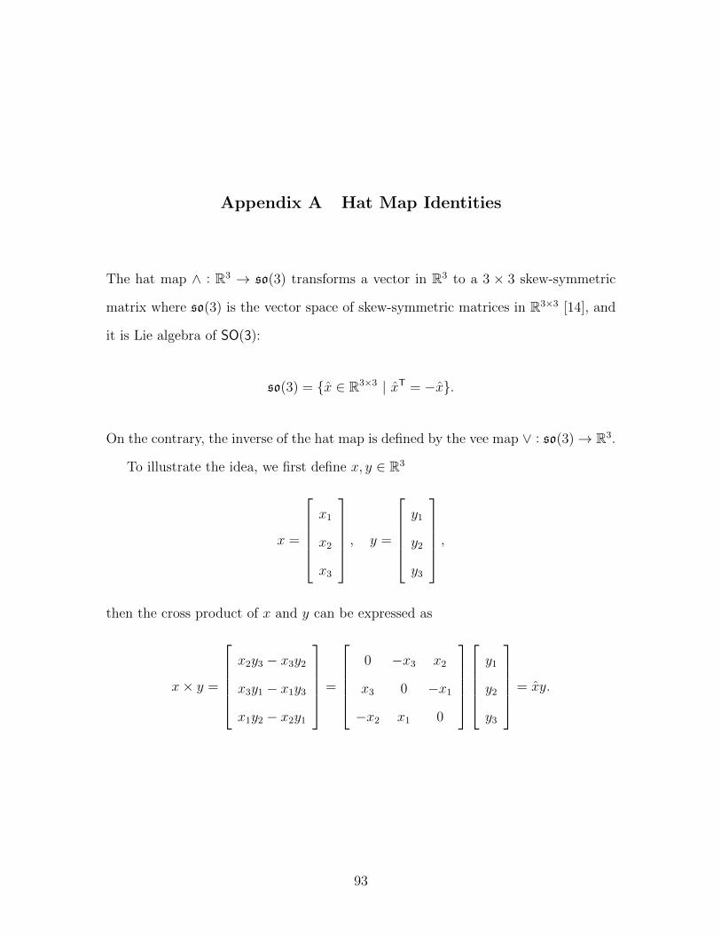
Appendix A Hat Map Identities

The hat map ∧ : R3 → so(3) transforms a vector in R3 to a 3 × 3 skew-symmetric

matrix where so(3) is the vector space of skew-symmetric matrices in R3×3 [14], and

it is Lie algebra of SO(3):

so(3) = x ∈ R3×3 | xT = −x.

On the contrary, the inverse of the hat map is defined by the vee map ∨ : so(3)→ R3.

To illustrate the idea, we first define x, y ∈ R3

x =

x1

x2

x3

, y =

y1

y2

y3

,

then the cross product of x and y can be expressed as

x× y =

x2y3 − x3y2

x3y1 − x1y3

x1y2 − x2y1

=

0 −x3 x2

x3 0 −x1

−x2 x1 0

y1

y2

y3

= xy.

93

Thus, we have

x =

0 −x3 x2

x3 0 −x1

−x2 x1 0

= −xT ∈ so(3). (A.1)

There are few properties of the hat map are summarized as follows:

xy = x× y = −y × x = −yx, (A.2)

x× y = xy − yx = yxT − xyT, (A.3)

RxRT = (Rx)∧, (A.4)

x · yz = y · zx = z · xy, (A.5)

xyz = x× (y × z) = (x · z)y − (x · y)z, (A.6)

xyz − zyx = yxz, (A.7)

1

2tr[xy] = −xTy, (A.8)

tr[xA] =1

2tr[x(A− AT)] = −xT(A− AT)∨, (A.9)

for any A ∈ R3×3, R ∈ SO(3). The sum of the diagonal entries of matrix A is equal

to the sum of eigenvalues of A and it is defined as trace of A, denoted by tr[A].

94

Appendix B The Spectral Theorem

From Chapter 5 of [48], the spectral theorem states the fact that any real symmetric

matrix K ∈ Rn×n can be factored into K = UGUT. It’s orthonormal eigenvectors

are column vectors of the orthogonal matrix U ∈ Rn×n and its eigenvalues are the

elements of diagonal of G ∈ Rn×n with every other elements are zero. The matrix

form of the spectral theorem can be specified as

K = UGUT =

| |

x1 · · · xn

| |

λ1

. . .

λn

− xT1 −

...

− xTn −

= λ1x1x

T1 + λ2x2x

T2 + · · ·+ λnxnx

Tn , (B.1)

where x1, x2,...xn ∈ Rn and λ1, λ2,...λn ∈ R are the orthonormal eigenvectors and

eigenvalues of a n by n symmetric matrix K, respectively.

95

Appendix C MATLAB Codes

The following is the MATLAB code for numerical simulation in Chapter 4.

function seven_spacecraft %% Main function %%

filename=’seven’;

close all;

global J1 J2 J3 J4 J5 J6 J7

global s12 s21 s23 s32 s34 s43 s45 s54 s56 s65 s67 s76

global s13 s24 s35 s47 s57 s75

global kO1 kO2 kO3 kO4 kO5 kO6 kO7

global K12a K12b K23a K23b K34a K34b K45a K45b K56a K56b K67a K67b

global cc12 cc23 cc34 cc45 cc56 cc67

J1=[3 0 0; 0 2 0; 0 0 1]; %Inertia matrix

J2=J1; J3=J1; J4=J1; J5=J1; J6=J1; J7=J1;

s1=[-1 0.1 0]’; s2=[-0.5 0 1/sqrt(2)]’; s3=[0.5 0 1/sqrt(2)]’;

s4=[1 0.1 0]’; s5=[0.5 0 -1/sqrt(2)]’; s6=[-0.5 0.0 -1/sqrt(2)]’;

s7=[0 0.2 0]’;

s12=(s2-s1)/norm(s2-s1); s13=(s3-s1)/norm(s3-s1);

s23=(s3-s2)/norm(s3-s2); s24=(s4-s2)/norm(s4-s2);

s34=(s4-s3)/norm(s4-s3); s35=(s5-s3)/norm(s5-s3);

s45=(s5-s4)/norm(s5-s4); s47=(s7-s4)/norm(s7-s4);

s56=(s6-s5)/norm(s6-s5); s57=(s7-s5)/norm(s7-s5);

s67=(s7-s6)/norm(s7-s6);

s21=-s12; s31=-s13;

s32=-s23; s42=-s24;

s43=-s34; s53=-s35;

s54=-s45; s74=-s47;

s65=-s56; s75=-s57; s76=-s67;

s123=cross(s12,s13); s213=cross(s21,s23); cc12=norm(s123)*norm(s213);

s234=cross(s23,s24); s324=cross(s32,s34); cc23=norm(s234)*norm(s324);

s345=cross(s34,s35); s435=cross(s43,s45); cc34=norm(s345)*norm(s435);

s457=cross(s45,s47); s547=cross(s54,s57); cc45=norm(s457)*norm(s547);

s567=cross(s56,s57); s657=cross(s65,s67); cc56=norm(s567)*norm(s657);

s675=cross(s67,s65); s765=cross(s76,s75); cc67=norm(s675)*norm(s765);

%k (w=3, eta=0.7, kO=2*eta*omega, ka=w^2)

96

w=5; eta=0.7;

kO1=2*w*eta; kO2=2*w*eta; kO3=2*w*eta; kO4=2*w*eta;

kO5=2*w*eta; kO6=2*w*eta; kO7=2*w*eta;

K12a=w^2; K12b=w^2+0.1; K23a=w^2; K23b=w^2+0.1;

K34a=w^2; K34b=w^2+0.1; K45a=w^2; K45b=w^2+0.1;

K56a=w^2; K56b=w^2+0.1; K67a=w^2; K67b=w^2+0.1;

tstart=0;

tend=20;

n=1001; %time step

tspan=linspace(tstart,tend,n);

%initial value of Omega1

OO1=[0 0 0].’; OO2=[0 0 0].’; OO3=[0 0 0].’; OO4=[0 0 0].’;

OO5=[0 0 0].’; OO6=[0 0 0].’; OO7=[0 0 0].’;

%initial value of R, it should still be a rotation matrix

RR1=[1 0 0 0 1 0 0 0 1].’;

RR2=[1 0 0 0 1 0 0 0 1].’;

RR3=reshape(expm(0.999*pi*hat([1 0 0])),9,1);

RR4=[1 0 0 0 1 0 0 0 1].’;

RR5=[1 0 0 0 1 0 0 0 1].’;

RR6=reshape(expm(0.999*pi*hat([0 1 0])),9,1);

RR7=[1 0 0 0 1 0 0 0 1].’;

xinit=[OO1;OO2;OO3;OO4;OO5;OO6;OO7;RR1;RR2;RR3;RR4;RR5;RR6;RR7];

OdeOption=odeset(’RelTol’,1e-8,’AbsTol’,1e-8);

[t,x]=ode45(@pid_SOTeom,tspan,xinit);

R1=zeros(3,3,n); R2=R1; R3=R1; R4=R1; R5=R1; R6=R1; R7=R1;

Q12d=R1; Q23d=R1; Q34d=R1; Q45d=R1; Q56d=R1; Q67d=R1;

dQ12d=R1; dQ23d=R1; dQ34d=R1; dQ45d=R1; dQ56d=R1; dQ67d=R1;

u1=zeros(3,n); u2=u1; u3=u1; u4=u1; u5=u1; u6=u1; u7=u1;

Omega12d=u1; Omega23d=u1; Omega34d=u1; Omega45d=u1; Omega56d=u1;

Omega67d=u1; dOmega12d=u1; dOmega23d=u1; dOmega34d=u1; dOmega45d=u1;

dOmega56d=u1; dOmega67d=u1;

eOM1=u1; eOM2=u1; eOM3=u1; eOM4=u1; eOM5=u1; eOM6=u1; eOM7=u1;

eQ12=u1; eQ23=u1; eQ34=u1; eQ45=u1; eQ56=u1; eQ67=u1;

Psi12=zeros(1,n); Psi23=Psi12; Psi34=Psi12; Psi45=Psi12;

Psi56=Psi12; Psi67=Psi12;

for k=1:n

R1(:,:,k)=reshape(x(k,22:30),3,3);

R2(:,:,k)=reshape(x(k,31:39),3,3);

R3(:,:,k)=reshape(x(k,40:48),3,3);

R4(:,:,k)=reshape(x(k,49:57),3,3);

R5(:,:,k)=reshape(x(k,58:66),3,3);

97

R6(:,:,k)=reshape(x(k,67:75),3,3);

R7(:,:,k)=reshape(x(k,76:84),3,3);

[Q12d(:,:,k) dQ12d(:,:,k) Omega12d(:,k) dOmega12d(:,k)...

Q23d(:,:,k) dQ23d(:,:,k) Omega23d(:,k) dOmega23d(:,k)...

Q34d(:,:,k) dQ34d(:,:,k) Omega34d(:,k) dOmega34d(:,k)...

Q45d(:,:,k) dQ45d(:,:,k) Omega45d(:,k) dOmega45d(:,k)...

Q56d(:,:,k) dQ56d(:,:,k) Omega56d(:,k) dOmega56d(:,k)...

Q67d(:,:,k) dQ67d(:,:,k) Omega67d(:,k) dOmega67d(:,k)]...

= desire(t(k));

[u1(:,k) u2(:,k) u3(:,k) u4(:,k) u5(:,k) u6(:,k) u7(:,k)...

Psi12(k) Psi23(k) Psi34(k) Psi45(k) Psi56(k) Psi67(k)...

eOM1(:,k) eOM2(:,k) eOM3(:,k) eOM4(:,k) ...

eOM5(:,k) eOM6(:,k) eOM7(:,k)...

eQ12(:,k) eQ23(:,k) eQ34(:,k)...

eQ45(:,k) eQ56(:,k) eQ67(:,k)...

Omega1d(:,k) Omega2d(:,k) Omega3d(:,k) Omega4d(:,k)...

Omega5d(:,k) Omega6d(:,k) Omega7d(:,k) dOmega1d(:,k)...

dOmega2d(:,k) dOmega3d(:,k) dOmega4d(:,k) dOmega5d(:,k)...

dOmega6d(:,k) dOmega7d(:,k)] = controller(t(k),x(k,:)’);

end

W1=x(:,1:3); W2=x(:,4:6); W3=x(:,7:9); W4=x(:,10:12);

W5=x(:,13:15); W6=x(:,16:18); W7=x(:,19:21);

figure;

plot(t,Psi12,t,Psi23,t,Psi34,t,Psi45,t,Psi56,t,Psi67);

figure;

for ff=1:3;

subplot(3,1,ff);

for aa=1:6;

eval([’plot(t,eOM’ num2str(aa) ’(’ num2str(ff) ’,:));’]);

hold on;

end

end

figure;

for ff=1:3;

subplot(3,1,ff);

for aa=1:5;

eval([’plot(t,eQ’ num2str(aa) num2str(aa+1)...

’(’ num2str(ff) ’,:));’]);

hold on;

end

end

98

save(filename);

evalin(’base’,’clear all;’)

evalin(’base’,[’load ’ filename ’;’]); % load results to workspace

end

%% Second Function

function [dx] = pid_SOTeom(t,x) %% Sub function %%

global J1 J2 J3 J4 J5 J6 J7;

%angular velocity, Omega(BFF)

Om1=x(1:3); Om2=x(4:6); Om3=x(7:9); Om4=x(10:12);

Om5=x(13:15); Om6=x(16:18); Om7=x(19:21);

%Omega1 hat

Om1h=hat(Om1); Om2h=hat(Om2); Om3h=hat(Om3); Om4h=hat(Om4);

Om5h=hat(Om5); Om6h=hat(Om6); Om7h=hat(Om7);

R1=reshape(x(22:30),3,3); %Rotation matrix

R2=reshape(x(31:39),3,3);

R3=reshape(x(40:48),3,3);

R4=reshape(x(49:57),3,3);

R5=reshape(x(58:66),3,3);

R6=reshape(x(67:75),3,3);

R7=reshape(x(76:84),3,3);

[u1 u2 u3 u4 u5 u6 u7]=controller(t,x);

%% Equation of Motion

dOm1=J1 (u1-cross(Om1,J1*Om1));

dOm2=J2 (u2-cross(Om2,J2*Om2));

dOm3=J3 (u3-cross(Om3,J3*Om3));

dOm4=J4 (u4-cross(Om4,J4*Om4));

dOm5=J5 (u5-cross(Om5,J5*Om5));

dOm6=J6 (u6-cross(Om6,J6*Om6));

dOm7=J7 (u7-cross(Om7,J7*Om7));

dR1=R1*Om1h; dR2=R2*Om2h; dR3=R3*Om3h; dR4=R4*Om4h;

dR5=R5*Om5h; dR6=R6*Om6h; dR7=R7*Om7h;

dR1a=reshape(dR1,9,1); dR2a=reshape(dR2,9,1);

dR3a=reshape(dR3,9,1); dR4a=reshape(dR4,9,1);

dR5a=reshape(dR5,9,1); dR6a=reshape(dR6,9,1);

dR7a=reshape(dR7,9,1);

dx=[dOm1;dOm2;dOm3;dOm4;dOm5;dOm6;dOm7;...

dR1a;dR2a;dR3a;dR4a;dR5a;dR6a;dR7a];

end

%% Sub-sub-routine

function [Q12d dQ12d Omega12d dOmega12d Q23d dQ23d Omega23d ...

dOmega23d Q34d dQ34d Omega34d dOmega34d Q45d dQ45d Omega45d...

99

dOmega45d Q56d dQ56d Omega56d dOmega56d Q67d dQ67d Omega67d...

dOmega67d]= desire(t)

Q12d=eye(3); dQ12d=zeros(3); Omega12d=[0 0 0]’; dOmega12d=[0 0 0]’;

Q23d=eye(3); dQ23d=zeros(3); Omega23d=[0 0 0]’; dOmega23d=[0 0 0]’;

% Euler angle: gamma beta alpha

alpha=sin(0.5*t); dalpha=0.5*cos(0.5*t); ddalpha=-(0.5^2)*sin(0.5*t);

beta=0.1; dbeta=0; ddbeta=0;

gamma=cos(t); dgamma=-sin(t); ddgamma=-cos(t);

[Q34d dQ34d Omega34d dOmega34d]=Eu2Rot(alpha,dalpha,ddalpha,...

beta,dbeta,ddbeta,gamma,dgamma,ddgamma);

alpha=0; dalpha=0; ddalpha=0;

beta=-0.1+cos(0.2*t); dbeta=-0.2*sin(0.2*t); ddbeta=-(0.2)^2*cos(0.2*t);

gamma=0.5*sin(2*t); dgamma=0.5*2*cos(2*t); ddgamma=-0.5*2*2*sin(2*t);

[Q45d dQ45d Omega45d dOmega45d]=Eu2Rot(alpha,dalpha,ddalpha,...

beta,dbeta,ddbeta,gamma,dgamma,ddgamma);

Q56d=eye(3); dQ56d=zeros(3); Omega56d=[0 0 0]’; dOmega56d=[0 0 0]’;

Q67d=Q45d’; dQ67d=dQ45d’; Omega67d=-Q67d’*Omega45d;

dOmega67d=-dQ67d’*Omega45d-Q67d’*dOmega45d;

end

function [Q dQ W dW]=...

Eu2Rot(alpha,dalpha,ddalpha,beta,dbeta,ddbeta,gamma,dgamma,ddgamma)

e1=[1 0 0]’; e2=[0 1 0]’; e3=[0 0 1]’;

he1=hat(e1); he2=hat(e2); he3=hat(e3); %e3 hat

ea=expm(gamma*he3); eb=expm(beta*he2); ec=expm(alpha*he1);

dea=(dgamma*he3)*ea; deb=(dbeta*he2)*eb; dec=(dalpha*he1)*ec;

ddea =(ddgamma*he3)*ea+(dgamma*he3)*dea;

ddeb =(ddbeta*he2)*eb+(dbeta*he2)*deb;

ddec =(ddalpha*he1)*ec+(dalpha*he1)*dec;

Q=ea*eb*ec;

dQ=dea*eb*ec + ea*deb*ec + ea*eb*dec;

ddQ1=ddea*eb*ec + dea*deb*ec + dea*eb*dec;

ddQ2=dea*deb*ec + ea*ddeb*ec + ea*deb*dec;

ddQ3=dea*eb*dec + ea*deb*dec + ea*eb*ddec;

ddQ =ddQ1+ddQ2+ddQ3;

100

W=vee(Q’*dQ);

dW=vee(dQ’*dQ+Q’*ddQ);

end

%% Controller

function [u1 u2 u3 u4 u5 u6 u7...

Psi12 Psi23 Psi34 Psi45 Psi56 Psi67...

eOM1 eOM2 eOM3 eOM4 eOM5 eOM6 eOM7...

eQ12 eQ23 eQ34 eQ45 eQ56 eQ67 ...

Omega1d Omega2d Omega3d Omega4d Omega5d Omega6d Omega7d ...

dOmega1d dOmega2d dOmega3d dOmega4d dOmega5d dOmega6d...

dOmega7d ] = controller(t,x)

global J1 J2 J3 J4 J5 J6 J7

global s12 s21 s23 s32 s34 s43 s45 s54 s56 s65 s67 s76

global s13 s24 s35 s47 s57 s75

global kO1 kO2 kO3 kO4 kO5 kO6 kO7

global K12a K12b K23a K23b K34a K34b K45a K45b K56a K56b K67a K67b

global VS MAGN BeaconLocs

global cc12 cc23 cc34 cc45 cc56 cc67

Om1=x(1:3); Om2=x(4:6); Om3=x(7:9); Om4=x(10:12); %Omega

Om5=x(13:15); Om6=x(16:18); Om7=x(19:21);

R1=reshape(x(22:30),3,3); %Rotation matrix

R2=reshape(x(31:39),3,3);

R3=reshape(x(40:48),3,3);

R4=reshape(x(49:57),3,3);

R5=reshape(x(58:66),3,3);

R6=reshape(x(67:75),3,3);

R7=reshape(x(76:84),3,3);

Q12=(R2.’)*R1; Q23=(R3.’)*R2; Q34=(R4.’)*R3; %Q

Q45=(R5.’)*R4; Q56=(R6.’)*R5; Q67=(R7.’)*R6;

[Q12d dQ12d Omega12d dOmega12d...

Q23d dQ23d Omega23d dOmega23d Q34d dQ34d Omega34d dOmega34d...

Q45d dQ45d Omega45d dOmega45d Q56d dQ56d Omega56d dOmega56d...

Q67d dQ67d Omega67d dOmega67d] = desire(t);

b12=(R1’)*s12; b13=(R1’)*s13;

b21=(R2’)*s21; b23=(R2’)*s23; b24=(R2’)*s24;

b32=(R3’)*s32; b34=(R3’)*s34; b35=(R3’)*s35;

b43=(R4’)*s43; b47=(R4’)*s47;

b45=(R4’)*s45;

b54=(R5’)*s54; b56=(R5’)*s56; b57=(R5’)*s57;

b65=(R6’)*s65; b67=(R6’)*s67;

b75=(R7’)*s75; b76=(R7’)*s76;

101

b123=cross(b12,b13); b213=cross(b21,b23);

psi12a=1-dot(b21,(-Q12d*b12)); psi12b=1-(1/cc12)*dot(Q12d*b123,-b213);

Psi12=(K12a*psi12a)+(K12b*psi12b);

b234=cross(b23,b24); b324=cross(b32,b34);

psi23a=1-dot(b32,(-Q23d*b23)); psi23b=1-(1/cc23)*dot(Q23d*b234,-b324);

Psi23=(K23a*psi23a)+(K23b*psi23b);

b345=cross(b34,b35); b435=cross(b43,b45);

psi34a=1-dot(b43,(-Q34d*b34)); psi34b=1-(1/cc34)*dot(Q34d*b345,-b435);

Psi34=(K34a*psi34a)+(K34b*psi34b);

b457=cross(b45,b47); b547=cross(b54,b57);

psi45a=1-dot(b54,(-Q45d*b45)); psi45b=1-(1/cc45)*dot(Q45d*b457,-b547);

Psi45=(K45a*psi45a)+(K45b*psi45b);

b567=cross(b56,b57); b657=cross(b65,b67);

psi56a=1-dot(b65,(-Q56d*b56)); psi56b=1-(1/cc56)*dot(Q56d*b567,-b657);

Psi56=(K56a*psi56a)+(K56b*psi56b);

b675=cross(b67,b65); b765=cross(b76,b75);

psi67a=1-dot(b76,(-Q67d*b67)); psi67b=1-(1/cc67)*dot(Q67d*b675,-b765);

Psi67=(K67a*psi67a)+(K67b*psi67b);

e12a = cross( ((Q12d.’)*b21),b12 ); %e_12^alpha

e21a = cross( (Q12d*b12),b21 ); %e_21^alpha

e12b = cross( ( (1/cc12)*(Q12d.’)*b213 ),b123 ); %e_12^beta

e21b = cross( ( (1/cc12)*Q12d*b123 ),b213 ); %e_21^beta

e12 = (K12a*e12a)+(K12b*e12b); %e_12

e21 = (K12a*e21a)+(K12b*e21b); %e_21

e23a = cross( ((Q23d.’)*b32),b23 ); %e_23^alpha

e32a = cross( (Q23d*b23),b32 );

e23b = cross( ((1/cc23)*(Q23d.’)*b324),b234 ); %e_23^beta

e32b = cross( ((1/cc23)*Q23d*b234),b324 ); %e_32^beta

e23 = (K23a*e23a)+(K23b*e23b); %e_23

e32 = (K23a*e32a)+(K23b*e32b); %e_32

e34a = cross( ((Q34d.’)*b43),b34 ); %e_34^alpha

e43a = cross( (Q34d*b34),b43 ); %e_43^alpha

e34b = cross( ( (1/cc34)*(Q34d.’)*b435 ),b345 ); %e_34^beta

e43b = cross( ( (1/cc34)*Q34d*b345 ),b435 ); %e_43^beta

e34 = (K34a*e34a)+(K34b*e34b); %e_34

e43 = (K34a*e43a)+(K34b*e43b); %e_43

102

e45a=cross(((Q45d.’)*b54),b45);

e54a=cross((Q45d*b45),b54);

e45b=cross(((1/cc45)*(Q45d.’)*b547),b457);

e54b=cross(((1/cc45)*Q45d*b457),b547);

e45 = (K45a*e45a)+(K45b*e45b);

e54 = (K45a*e54a)+(K45b*e54b);

e56a = cross( ((Q56d.’)*b65),b56 );

e65a = cross( (Q56d*b56),b65 );

e56b = cross( ( (1/cc56)*(Q56d.’)*b657 ),b567 );

e65b = cross( ( (1/cc56)*Q56d*b567 ),b657 );

e56 = (K56a*e56a)+(K56b*e56b);

e65 = (K56a*e65a)+(K56b*e65b);

e67a = cross( ((Q67d.’)*b76),b67 );

e76a = cross( (Q67d*b67),b76 );

e67b = cross( ( (1/cc67)*(Q67d.’)*b765 ),b675 );

e76b = cross( ( (1/cc67)*Q67d*b675 ),b765 );

e67 = (K67a*e67a)+(K67b*e67b);

e76 = (K67a*e76a)+(K67b*e76b);

Omega3d=Omega34d; dOmega3d=dOmega34d;

Omega4d=[0 0 0]’; dOmega4d=[0 0 0]’;

Omega2d=Q23d’*Omega3d; dOmega2d=dQ23d’*Omega3d+Q23d’*dOmega3d;

Omega1d=Q12d’*Omega2d; dOmega1d=dQ12d’*Omega2d+Q12d’*dOmega2d;

Omega5d=-Q45d*Omega45d; dOmega5d=-dQ45d*Omega45d-Q45d*dOmega45d;

Omega6d=Q56d*Omega5d; dOmega6d=dQ56d*Omega5d+Q56d*dOmega5d;

Omega7d=Q67d*(Omega6d-Omega67d);

dOmega7d=dQ67d*(Omega6d-Omega67d)+Q67d*(dOmega6d-dOmega67d);

eOM1=Om1-Omega1d; eOM2=Om2-Omega2d; eOM3=Om3-Omega3d;

eOM4=Om4-Omega4d; eOM5=Om5-Omega5d; eOM6=Om6-Omega6d;

eOM7=Om7-Omega7d;

A1=cross(Omega1d, J1*(eOM1+Omega1d));

A2=cross(Omega2d, J2*(eOM2+Omega2d));

A3=cross(Omega3d, J3*(eOM3+Omega3d));

A4=cross(Omega4d, J4*(eOM4+Omega4d));

A5=cross(Omega5d, J5*(eOM5+Omega5d));

A6=cross(Omega6d, J2*(eOM6+Omega6d));

A7=cross(Omega7d, J7*(eOM7+Omega7d));

B1=J1*dOmega1d; B2=J2*dOmega2d; B3=J3*dOmega3d; B4=J4*dOmega4d;

B5=J5*dOmega5d; B6=J6*dOmega6d; B7=J7*dOmega7d;

u1=-e12-kO1*eOM1+A1+B1; u7=-e76-kO7*eOM7+A7+B7;

103

u2=-(e21+e23)/2-kO2*eOM2+A2+B2; u3=-(e32+e34)/2-kO3*eOM3+A3+B3;

u4=-(e43+e45)/2-kO4*eOM4+A4+B4; u5=-(e54+e56)/2-kO5*eOM5+A5+B5;

u6=-(e65+e67)/2-kO6*eOM6+A6+B6;

eQ12=vee( 1/2*( (Q12d.’)*Q12-(Q12.’)*Q12d ) );

eQ23=vee( 1/2*( (Q23d.’)*Q23-(Q23.’)*Q23d ) );

eQ34=vee( 1/2*( (Q34d.’)*Q34-(Q34.’)*Q34d ) );

eQ45=vee( 1/2*( (Q45d.’)*Q45-(Q45.’)*Q45d ) );

eQ56=vee( 1/2*( (Q56d.’)*Q56-(Q56.’)*Q56d ) );

eQ67=vee( 1/2*( (Q67d.’)*Q67-(Q67.’)*Q67d ) );

end

function x=vee(X)

x=[X(3,2) X(1,3) X(2,1)]’;

end

function Y=hat(y)

Y=[0 -y(3) y(2); y(3) 0 -y(1); -y(2) y(1) 0];

end

104