space-time adaptive processing: fundamentals

Space-Time Adaptive Processing: Fundamentals

Wolfram Bürger Research Institute for High-Frequency Physics and Radar Techniques (FHR)

Research Establishment for Applied Science (FGAN) Neuenahrer Str. 20, D-53343 Wachtberg

GERMANY

[email protected]

ABSTRACT

In this lecture, we present the principles of space-time adaptive processing (STAP) for radar, applied to moving target indication. We discuss the properties of optimum STAP, as well as problems associated with estimating the adaptive weights not encountered with spatial-only processing (i.e. beamforming).

1 INTRODUCTION

1.1 Space-Time Adaptive Processing for Moving Target Indication Moving target indication (MTI) is a common radar mission involving the detection of airborne or ground moving targets. It is based on the fact that the radar echoes of moving targets are Doppler shifted. The Doppler frequency

λrad

Dvf 2

−= (1)

of a target echo depends on the radial velocity radv between the radar and the target, and on the wavelength λ at which the radar system is transmitting. If the radar is not moving, a simple high-pass Doppler filter is obviously sufficient for suppressing clutter echoes, i.e. the echoes of stationary scatterers.

If the radar platform is moving, the clutter echoes are Doppler shifted as well. However, in contrast to the radar echoes from moving targets, the Doppler shift of the clutter echoes is solely due to the platform motion. Surfaces of constant radial velocity – and thus constant clutter Doppler frequency – are cones about the direction of flight. The Doppler frequency of an individual clutter scatterer echo is given by

βλ

cos2 PD

vf = , (2)

where Pv denotes the platform velocity, and β

R

is the (cone) angle between the flight direction and the direction of the scatterer.

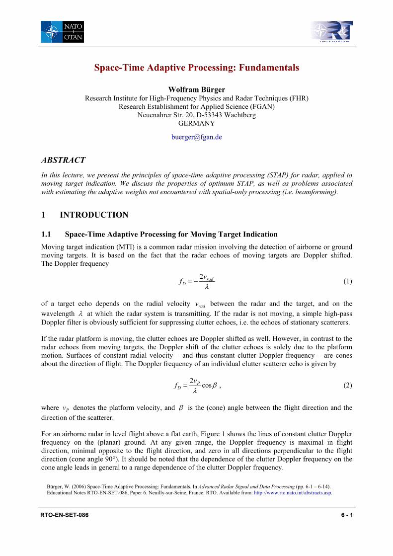
For an airborne radar in level flight above a flat earth, Figure 1 shows the lines of constant clutter Doppler frequency on the (planar) ground. At any given range, the Doppler frequency is maximal in flight direction, minimal opposite to the flight direction, and zero in all directions perpendicular to the flight direction (cone angle 90°). It should be noted that the dependence of the clutter Doppler frequency on the cone angle leads in general to a range dependence of the clutter Doppler frequency.

Bürger, W. (2006) Space-Time Adaptive Processing: Fundamentals. In Advanced Radar Signal and Data Processing (pp. 6-1 – 6-14). Educational Notes RTO-EN-SET-086, Paper 6. Neuilly-sur-Seine, France: RTO. Available from: http://www.rto.nato.int/abstracts.asp.

TO-EN-SET-086 6 - 1

http://www.rto.nato.int/abstracts.asp

Report Documentation Page Form ApprovedOMB No. 0704-0188

Public reporting burden for the collection of information is estimated to average 1 hour per response, including the time for reviewing instructions, searching existing data sources, gathering andmaintaining the data needed, and completing and reviewing the collection of information. Send comments regarding this burden estimate or any other aspect of this collection of information,including suggestions for reducing this burden, to Washington Headquarters Services, Directorate for Information Operations and Reports, 1215 Jefferson Davis Highway, Suite 1204, ArlingtonVA 22202-4302. Respondents should be aware that notwithstanding any other provision of law, no person shall be subject to a penalty for failing to comply with a collection of information if itdoes not display a currently valid OMB control number.

1. REPORT DATE 01 SEP 2006

2. REPORT TYPE N/A

3. DATES COVERED -

4. TITLE AND SUBTITLE Space-Time Adaptive Processing: Fundamentals

5a. CONTRACT NUMBER

5b. GRANT NUMBER

5c. PROGRAM ELEMENT NUMBER

6. AUTHOR(S) 5d. PROJECT NUMBER

5e. TASK NUMBER

5f. WORK UNIT NUMBER

7. PERFORMING ORGANIZATION NAME(S) AND ADDRESS(ES) Research Institute for High-Frequency Physics and Radar Techniques(FHR) Research Establishment for Applied Science (FGAN) NeuenahrerStr. 20, D-53343 Wachtberg GERMANY

8. PERFORMING ORGANIZATIONREPORT NUMBER

9. SPONSORING/MONITORING AGENCY NAME(S) AND ADDRESS(ES) 10. SPONSOR/MONITOR’S ACRONYM(S)

11. SPONSOR/MONITOR’S REPORT NUMBER(S)

12. DISTRIBUTION/AVAILABILITY STATEMENT Approved for public release, distribution unlimited

13. SUPPLEMENTARY NOTES See also ADM001925, Advanced Radar Signal and Data Processing., The original document contains color images.

14. ABSTRACT

15. SUBJECT TERMS

16. SECURITY CLASSIFICATION OF: 17. LIMITATION OF ABSTRACT

UU

18. NUMBEROF PAGES

14

19a. NAME OFRESPONSIBLE PERSON

a. REPORT unclassified

b. ABSTRACT unclassified

c. THIS PAGE unclassified

Standard Form 298 (Rev. 8-98) Prescribed by ANSI Std Z39-18

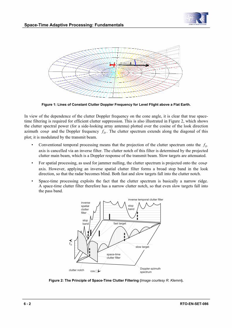
Figure 1: Lines of Constant Clutter Doppler Frequency for Level Flight above a Flat Earth.

In view of the dependence of the clutter Doppler frequency on the cone angle, it is clear that true space-time filtering is required for efficient clutter suppression. This is also illustrated in Figure 2, which shows the clutter spectral power (for a side-looking array antenna) plotted over the cosine of the look direction azimuth ϕcos and the Doppler frequency Df . The clutter spectrum extends along the diagonal of this plot; it is modulated by the transmit beam.

• Conventional temporal processing means that the projection of the clutter spectrum onto the Df axis is cancelled via an inverse filter. The clutter notch of this filter is determined by the projected clutter main beam, which is a Doppler response of the transmit beam. Slow targets are attenuated.

• For spatial processing, as used for jammer nulling, the clutter spectrum is projected onto the ϕcos axis. However, applying an inverse spatial clutter filter forms a broad stop band in the look direction, so that the radar becomes blind. Both fast and slow targets fall into the clutter notch.

• Space-time processing exploits the fact that the clutter spectrum is basically a narrow ridge. A space-time clutter filter therefore has a narrow clutter notch, so that even slow targets fall into the pass band.

��

��

��

��

��

��

��

��

��

�

��

Figure 2: The Principle of Space-Time Clutter Filtering (Image courtesy R. Klemm).


6 - 2 RTO-EN-SET-086

1.2 Other Applications of Space-Time Processing Besides clutter suppression, numerous other applications of space-time processing are known [4], e.g.

• Interference suppression for broadband radar,

• Suppression of terrain scattered jamming (in radar),

• Suppression of reverberation in active sonar,

• Simultaneous localisation and Doppler estimation for passive sonar (matched field processing),

• Signal processing for communications networks,

• Wideband interference rejection in GPS arrays.

2 OPTIMUM SPACE-TIME ADAPTIVE PROCESSING

2.1 Spatial and Temporal (Doppler) Filtering Although the beamforming operation for phased arrays has already been described in [5], we recall here briefly the main results to show the similarity of beamforming and Doppler filtering.

To sum all signals arriving at the elements of a phased array coherently, the time delay of the signal received at the antenna element at position Tzyx ),,(=r has to be compensated. Denoting the angle of incidence of an incoming plane wave by the unit direction vector u in the antenna coordinate system, the signal at element r can be written as

cfjtfj Teebts /22),( ur

r u ππ⋅= , (3)

where f is the transmit frequency of the radar and c the speed of light. Correspondingly, a beam into a direction 0u with N antenna elements is formed by compensating these delays by

),()(),(),( 01 )(

/20

0

0 usuauuu ru

ur ttsetS HN

n a

cfjn

n

Tn =⋅=− ∑

=

−43421

π . (4)

Now consider a radar transmitting a train of M coherent pulses. To sum all signals arriving at the radar coherently, the phase change due to the Doppler frequency of the signal received at time T has to be compensated. Denoting the Doppler frequency of the received signal by Df , the signal received at time T can be written as

Tfjtfj

tTfjtfjDT

D

D

eeb

eebftsππ

ππ

22

)(22),(

⋅≈

⋅= +

(5)

if 1<<tfD . Correspondingly, a Doppler filter for the Doppler frequency 0f is formed by compensating these phase changes by

),()(),(),( 01 )(

20

0D

HM

mDT

fa

TfjD ftfftsefftS

m

Dm

m sa=⋅=− ∑=

−43421

π . (6)


RTO-EN-SET-086 6 - 3

For a phased array radar transmitting a train of M coherent pulses, the beamforming and Doppler filtering operation can be combined into a space-time filtering operation

),,(),(),,( 0000 DH

D ftffftS usuauu =−− , (7)

where ( )TMNMN ssss LLLL 1111=s denotes the space-time signal vector and ( )TMNaa L11=a the space-time filter vector.

2.2 Optimum Space-Time Adaptive Processing If the interference situation (clutter, jamming, noise) is known, the optimum space-time adaptive filter vector w can be determined similar to the optimum beamforming vector in the case of spatial-only processing [5]. The probability of detection is maximised if the weight vector w is chosen so that it maximises the signal-to-noise-plus-interference ratio (SNIR) for a given signal ),( 000 fuaa =

Qww

waaw

njcw

awH

HH

H

H

ESNIR 00

2

20

)(=

++

= . (8)

The solution of this optimisation is

),( 001 fuaQw −= µ , (9)

where

{ }HE ))(( njcnjcQ ++++= (10)

is the space-time clutter-plus-jamming-plus-noise covariance matrix, and µ is a normalisation constant which can be chosen arbitrarily.

When comparing the performance of different processing techniques, it is convenient to study the SNIR loss [1]

00

000000

0 Naaaaaa

Qwwwaaw

H

HH

H

HH

SNRSNIR

= , (11)

i.e. the ratio of the output SNIR to the maximum signal-to-noise ratio 0SNR that can be achieved by the ideal matched filter for the interference-free case (thermal noise only). A SNIR loss of unity (0 dB) indicates perfect interference cancellation or no loss due to the presence of clutter and/or jamming.

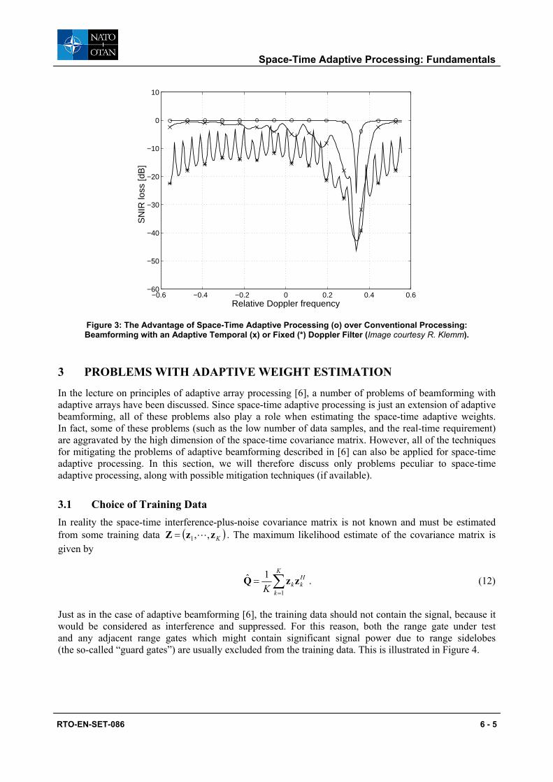
Figure 3 illustrates the advantage of optimum space-time adaptive processing (o) over conventional processing techniques, namely beamforming cascaded with optimum temporal clutter filtering (x), and simple beamforming plus Doppler filtering (*). For all three processors, the SNIR loss is plotted versus the relative Doppler frequency ( )PD vfF 2λ⋅= .



−0.6 −0.4 −0.2 0 0.2 0.4 0.6−60

−50

−40

−30

−20

−10

0

10

Relative Doppler frequency

SN

IR lo

ss [d

B]

Figure 3: The Advantage of Space-Time Adaptive Processing (o) over Conventional Processing: Beamforming with an Adaptive Temporal (x) or Fixed (*) Doppler Filter (Image courtesy R. Klemm).

3 PROBLEMS WITH ADAPTIVE WEIGHT ESTIMATION

In the lecture on principles of adaptive array processing [6], a number of problems of beamforming with adaptive arrays have been discussed. Since space-time adaptive processing is just an extension of adaptive beamforming, all of these problems also play a role when estimating the space-time adaptive weights. In fact, some of these problems (such as the low number of data samples, and the real-time requirement) are aggravated by the high dimension of the space-time covariance matrix. However, all of the techniques for mitigating the problems of adaptive beamforming described in [6] can also be applied for space-time adaptive processing. In this section, we will therefore discuss only problems peculiar to space-time adaptive processing, along with possible mitigation techniques (if available).

3.1 Choice of Training Data In reality the space-time interference-plus-noise covariance matrix is not known and must be estimated from some training data ( )KzzZ ,,1 L= . The maximum likelihood estimate of the covariance matrix is given by

∑=

=K

k

HkkK 1

1ˆ zzQ . (12)

Just as in the case of adaptive beamforming [6], the training data should not contain the signal, because it would be considered as interference and suppressed. For this reason, both the range gate under test and any adjacent range gates which might contain significant signal power due to range sidelobes (the so-called “guard gates”) are usually excluded from the training data. This is illustrated in Figure 4.



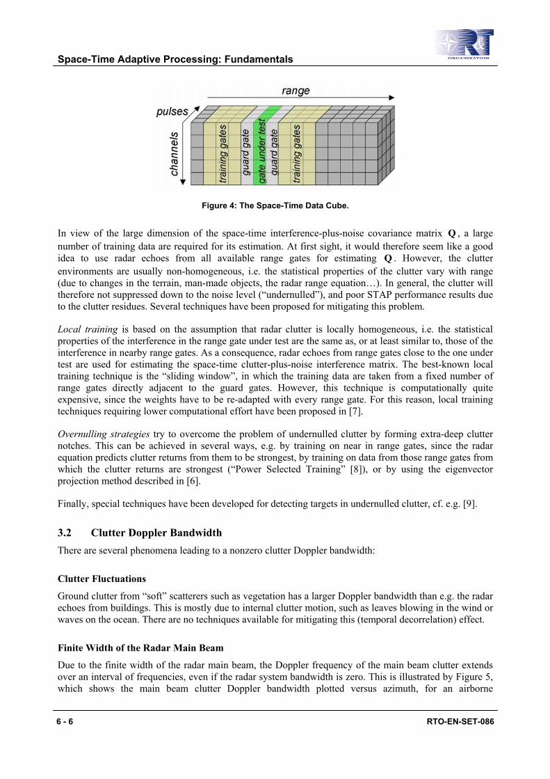
Figure 4: The Space-Time Data Cube.

In view of the large dimension of the space-time interference-plus-noise covariance matrix Q , a large number of training data are required for its estimation. At first sight, it would therefore seem like a good idea to use radar echoes from all available range gates for estimating Q . However, the clutter environments are usually non-homogeneous, i.e. the statistical properties of the clutter vary with range (due to changes in the terrain, man-made objects, the radar range equation…). In general, the clutter will therefore not suppressed down to the noise level (“undernulled”), and poor STAP performance results due to the clutter residues. Several techniques have been proposed for mitigating this problem.

Local training is based on the assumption that radar clutter is locally homogeneous, i.e. the statistical properties of the interference in the range gate under test are the same as, or at least similar to, those of the interference in nearby range gates. As a consequence, radar echoes from range gates close to the one under test are used for estimating the space-time clutter-plus-noise interference matrix. The best-known local training technique is the “sliding window”, in which the training data are taken from a fixed number of range gates directly adjacent to the guard gates. However, this technique is computationally quite expensive, since the weights have to be re-adapted with every range gate. For this reason, local training techniques requiring lower computational effort have been proposed in [7].

Overnulling strategies try to overcome the problem of undernulled clutter by forming extra-deep clutter notches. This can be achieved in several ways, e.g. by training on near in range gates, since the radar equation predicts clutter returns from them to be strongest, by training on data from those range gates from which the clutter returns are strongest (“Power Selected Training” [8]), or by using the eigenvector projection method described in [6].

Finally, special techniques have been developed for detecting targets in undernulled clutter, cf. e.g. [9].

3.2 Clutter Doppler Bandwidth There are several phenomena leading to a nonzero clutter Doppler bandwidth:

Clutter Fluctuations

Ground clutter from “soft” scatterers such as vegetation has a larger Doppler bandwidth than e.g. the radar echoes from buildings. This is mostly due to internal clutter motion, such as leaves blowing in the wind or waves on the ocean. There are no techniques available for mitigating this (temporal decorrelation) effect.

Finite Width of the Radar Main Beam

Due to the finite width of the radar main beam, the Doppler frequency of the main beam clutter extends over an interval of frequencies, even if the radar system bandwidth is zero. This is illustrated by Figure 5, which shows the main beam clutter Doppler bandwidth plotted versus azimuth, for an airborne



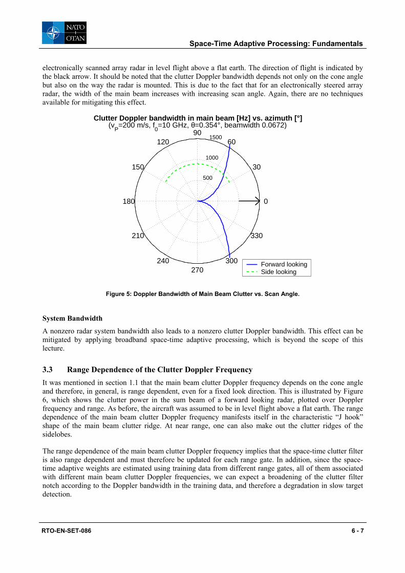
electronically scanned array radar in level flight above a flat earth. The direction of flight is indicated by the black arrow. It should be noted that the clutter Doppler bandwidth depends not only on the cone angle but also on the way the radar is mounted. This is due to the fact that for an electronically steered array radar, the width of the main beam increases with increasing scan angle. Again, there are no techniques available for mitigating this effect.

500

1000

1500

30

210

60

240

90

270

120

300

150

330

180 0

Clutter Doppler bandwidth in main beam [Hz] vs. azimuth [°](v

P=200 m/s, f

0=10 GHz, θ=0.354°, beamwidth 0.0672)

Forward lookingSide looking

Figure 5: Doppler Bandwidth of Main Beam Clutter vs. Scan Angle.

System Bandwidth

A nonzero radar system bandwidth also leads to a nonzero clutter Doppler bandwidth. This effect can be mitigated by applying broadband space-time adaptive processing, which is beyond the scope of this lecture.

3.3 Range Dependence of the Clutter Doppler Frequency It was mentioned in section 1.1 that the main beam clutter Doppler frequency depends on the cone angle and therefore, in general, is range dependent, even for a fixed look direction. This is illustrated by Figure 6, which shows the clutter power in the sum beam of a forward looking radar, plotted over Doppler frequency and range. As before, the aircraft was assumed to be in level flight above a flat earth. The range dependence of the main beam clutter Doppler frequency manifests itself in the characteristic “J hook” shape of the main beam clutter ridge. At near range, one can also make out the clutter ridges of the sidelobes.

The range dependence of the main beam clutter Doppler frequency implies that the space-time clutter filter is also range dependent and must therefore be updated for each range gate. In addition, since the space-time adaptive weights are estimated using training data from different range gates, all of them associated with different main beam clutter Doppler frequencies, we can expect a broadening of the clutter filter notch according to the Doppler bandwidth in the training data, and therefore a degradation in slow target detection.



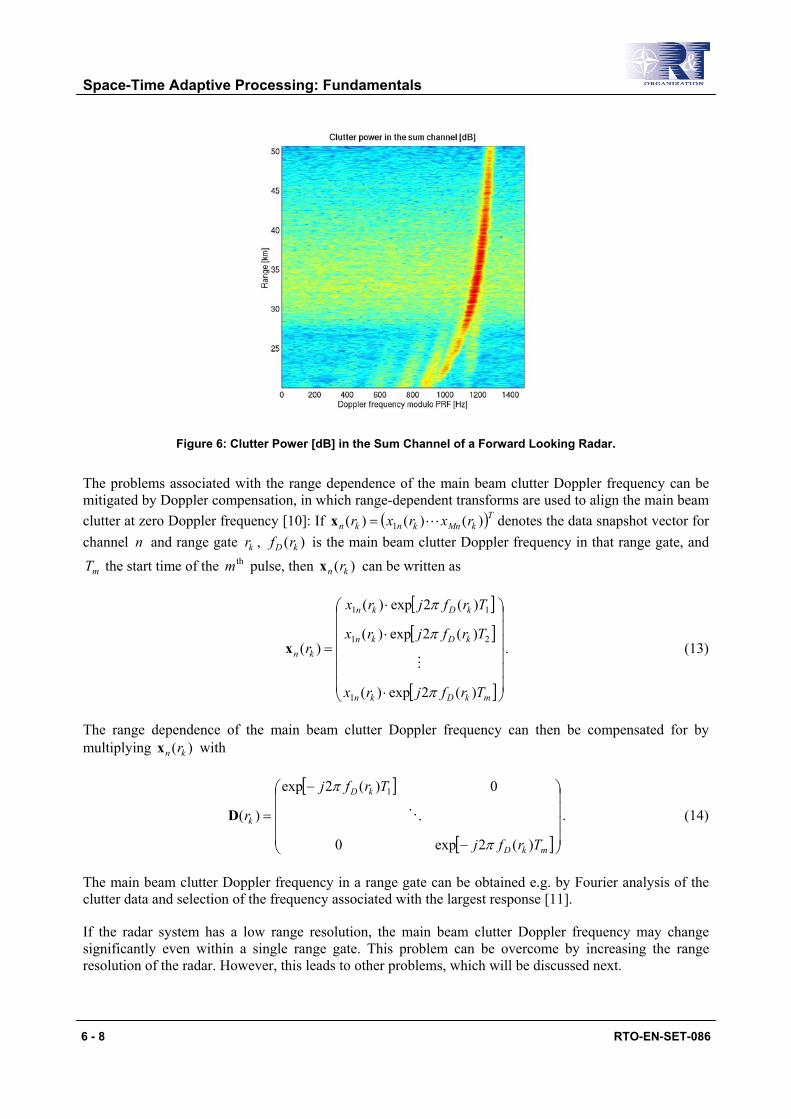
Figure 6: Clutter Power [dB] in the Sum Channel of a Forward Looking Radar.

The problems associated with the range dependence of the main beam clutter Doppler frequency can be mitigated by Doppler compensation, in which range-dependent transforms are used to align the main beam clutter at zero Doppler frequency [10]: If ( )TkMnknkn rxrxr )()()( 1 L=x denotes the data snapshot vector for channel n and range gate kr , )( kD rf is the main beam clutter Doppler frequency in that range gate, and

mT the start time of the thm pulse, then )( kn rx can be written as

[ ][ ]

[ ]

⋅

⋅

⋅

=

mkDkn

kDkn

kDkn

kn

Trfjrx

Trfjrx

Trfjrx

r

)(2exp)(

)(2exp)(

)(2exp)(

)(

1

21

11

π

π

π

Mx . (13)

The range dependence of the main beam clutter Doppler frequency can then be compensated for by multiplying )( kn rx with

[ ]

[ ]

−

−

=

mkD

kD

k

Trfj

Trfj

r

)(2exp0

0)(2exp

)(

1

π

π

OD . (14)

The main beam clutter Doppler frequency in a range gate can be obtained e.g. by Fourier analysis of the clutter data and selection of the frequency associated with the largest response [11].

If the radar system has a low range resolution, the main beam clutter Doppler frequency may change significantly even within a single range gate. This problem can be overcome by increasing the range resolution of the radar. However, this leads to other problems, which will be discussed next.



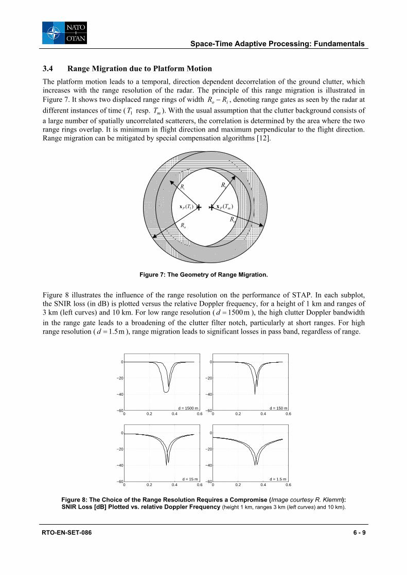
3.4 Range Migration due to Platform Motion The platform motion leads to a temporal, direction dependent decorrelation of the ground clutter, which increases with the range resolution of the radar. The principle of this range migration is illustrated in Figure 7. It shows two displaced range rings of width io RR − , denoting range gates as seen by the radar at different instances of time ( 1T resp. mT ). With the usual assumption that the clutter background consists of a large number of spatially uncorrelated scatterers, the correlation is determined by the area where the two range rings overlap. It is minimum in flight direction and maximum perpendicular to the flight direction. Range migration can be mitigated by special compensation algorithms [12].

Figure 7: The Geometry of Range Migration.

Figure 8 illustrates the influence of the range resolution on the performance of STAP. In each subplot, the SNIR loss (in dB) is plotted versus the relative Doppler frequency, for a height of 1 km and ranges of 3 km (left curves) and 10 km. For low range resolution ( m1500=d ), the high clutter Doppler bandwidth in the range gate leads to a broadening of the clutter filter notch, particularly at short ranges. For high range resolution ( m5.1=d ), range migration leads to significant losses in pass band, regardless of range.

0 0.2 0.4 0.6−60

−40

−20

0

d = 1500 m0 0.2 0.4 0.6

−60

−40

−20

0

d = 150 m

0 0.2 0.4 0.6−60

−40

−20

0

d = 15 m0 0.2 0.4 0.6

−60

−40

−20

0

d = 1.5 m

Figure 8: The Choice of the Range Resolution Requires a Compromise (Image courtesy R. Klemm): SNIR Loss [dB] Plotted vs. relative Doppler Frequency (height 1 km, ranges 3 km (left curves) and 10 km).

iR iR

oRoR

)( 1TPx )( mP Tx



3.5 Ambiguities in Range and Doppler

Doppler Ambiguities

If a radar uses a constant pulse repetition frequency (PRF), the velocity of a target cannot be determined unambiguously. In addition, the clutter suppression will also lead to the suppression of moving target echoes with certain radial velocities, the so-called blind velocities, which can be calculated from (1) to be

),2,1(2

K±±=⋅⋅= kPRFkvblindλ . (15)

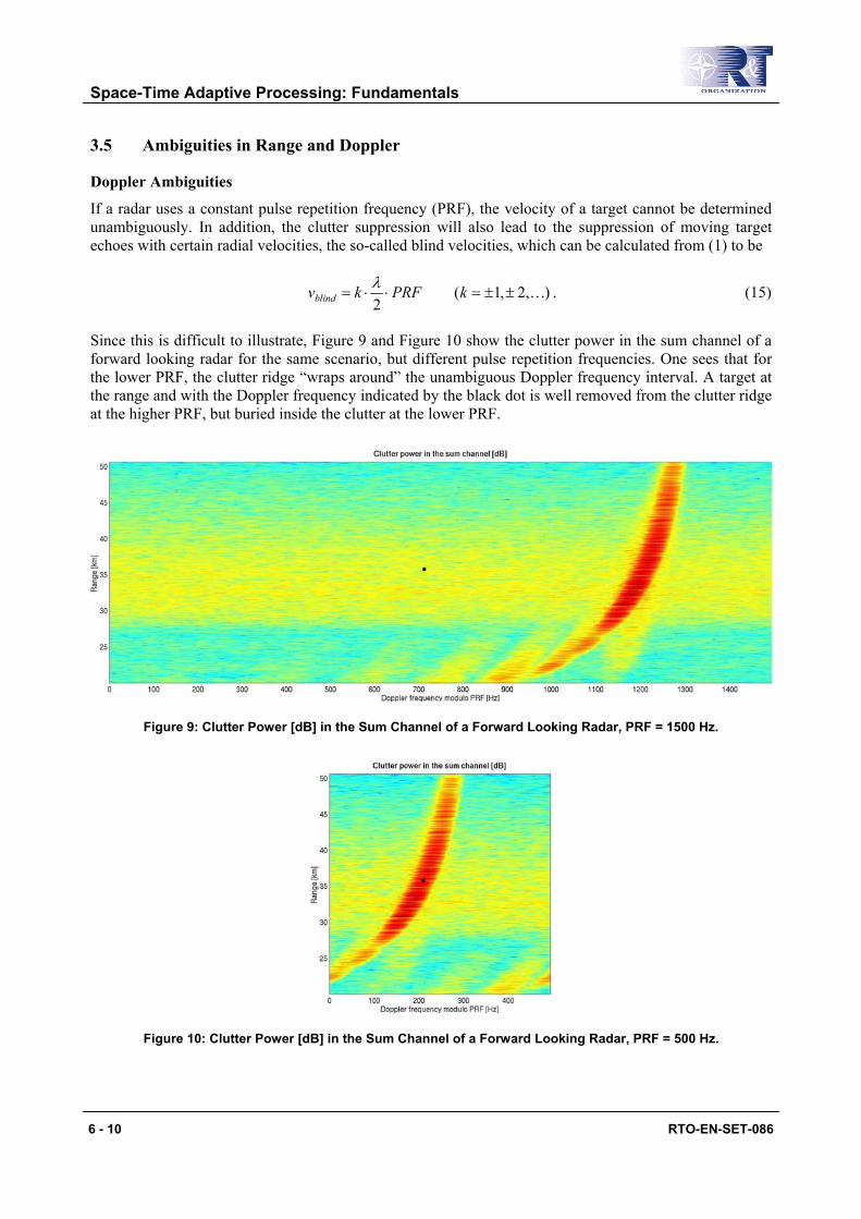
Since this is difficult to illustrate, Figure 9 and Figure 10 show the clutter power in the sum channel of a forward looking radar for the same scenario, but different pulse repetition frequencies. One sees that for the lower PRF, the clutter ridge “wraps around” the unambiguous Doppler frequency interval. A target at the range and with the Doppler frequency indicated by the black dot is well removed from the clutter ridge at the higher PRF, but buried inside the clutter at the lower PRF.

Figure 9: Clutter Power [dB] in the Sum Channel of a Forward Looking Radar, PRF = 1500 Hz.

Figure 10: Clutter Power [dB] in the Sum Channel of a Forward Looking Radar, PRF = 500 Hz.


6 - 10 RTO-EN-SET-086

Range Ambiguities

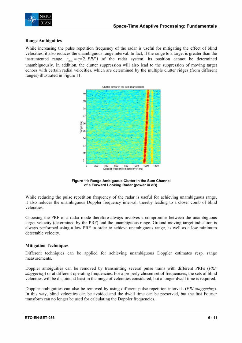
While increasing the pulse repetition frequency of the radar is useful for mitigating the effect of blind velocities, it also reduces the unambiguous range interval. In fact, if the range to a target is greater than the instrumented range ( )PRFcr ⋅= 2max of the radar system, its position cannot be determined unambiguously. In addition, the clutter suppression will also lead to the suppression of moving target echoes with certain radial velocities, which are determined by the multiple clutter ridges (from different ranges) illustrated in Figure 11.

Figure 11: Range Ambiguous Clutter in the Sum Channel of a Forward Looking Radar (power in dB).

While reducing the pulse repetition frequency of the radar is useful for achieving unambiguous range, it also reduces the unambiguous Doppler frequency interval, thereby leading to a closer comb of blind velocities.

Choosing the PRF of a radar mode therefore always involves a compromise between the unambiguous target velocity (determined by the PRF) and the unambiguous range. Ground moving target indication is always performed using a low PRF in order to achieve unambiguous range, as well as a low minimum detectable velocity.

Mitigation Techniques

Different techniques can be applied for achieving unambiguous Doppler estimates resp. range measurements.

Doppler ambiguities can be removed by transmitting several pulse trains with different PRFs (PRF staggering) or at different operating frequencies. For a properly chosen set of frequencies, the sets of blind velocities will be disjoint, at least in the range of velocities considered, but a longer dwell time is required.

Doppler ambiguities can also be removed by using different pulse repetition intervals (PRI staggering). In this way, blind velocities can be avoided and the dwell time can be preserved, but the fast Fourier transform can no longer be used for calculating the Doppler frequencies.


RTO-EN-SET-086 6 - 11

Range ambiguities can be avoided by employing an array antenna with vertical adaptivity (or at least a narrow main beam width in elevation).

Range ambiguities can also be avoided by coding the transmitted signal, so that radar echoes from an earlier pulse will not gain power by the pulse compression.

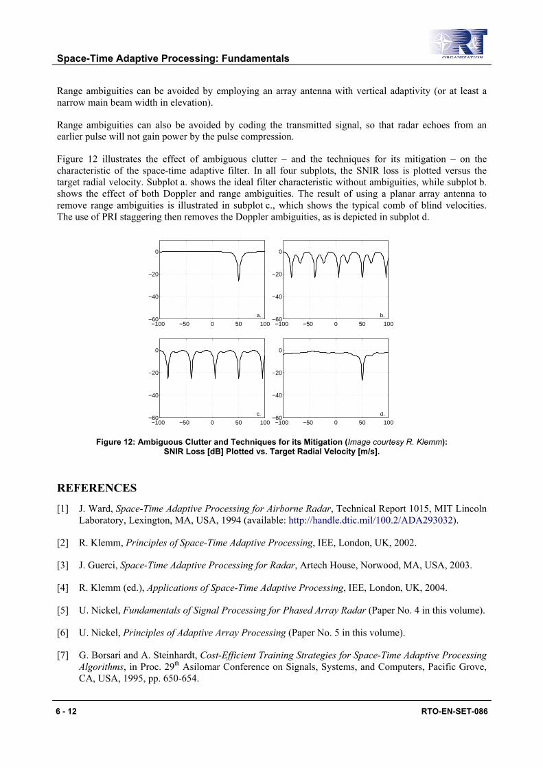
Figure 12 illustrates the effect of ambiguous clutter – and the techniques for its mitigation – on the characteristic of the space-time adaptive filter. In all four subplots, the SNIR loss is plotted versus the target radial velocity. Subplot a. shows the ideal filter characteristic without ambiguities, while subplot b. shows the effect of both Doppler and range ambiguities. The result of using a planar array antenna to remove range ambiguities is illustrated in subplot c., which shows the typical comb of blind velocities. The use of PRI staggering then removes the Doppler ambiguities, as is depicted in subplot d.

−100 −50 0 50 100−60

−40

−20

0

a.

−100 −50 0 50 100−60

−40

−20

0

b.

−100 −50 0 50 100−60

−40

−20

0

c.

−100 −50 0 50 100−60

−40

−20

0

d.

Figure 12: Ambiguous Clutter and Techniques for its Mitigation (Image courtesy R. Klemm): SNIR Loss [dB] Plotted vs. Target Radial Velocity [m/s].

REFERENCES

[1] J. Ward, Space-Time Adaptive Processing for Airborne Radar, Technical Report 1015, MIT Lincoln Laboratory, Lexington, MA, USA, 1994 (available: http://handle.dtic.mil/100.2/ADA293032).

[2] R. Klemm, Principles of Space-Time Adaptive Processing, IEE, London, UK, 2002.

[3] J. Guerci, Space-Time Adaptive Processing for Radar, Artech House, Norwood, MA, USA, 2003.

[4] R. Klemm (ed.), Applications of Space-Time Adaptive Processing, IEE, London, UK, 2004.

[5] U. Nickel, Fundamentals of Signal Processing for Phased Array Radar (Paper No. 4 in this volume).

[6] U. Nickel, Principles of Adaptive Array Processing (Paper No. 5 in this volume).

[7] G. Borsari and A. Steinhardt, Cost-Efficient Training Strategies for Space-Time Adaptive Processing Algorithms, in Proc. 29th Asilomar Conference on Signals, Systems, and Computers, Pacific Grove, CA, USA, 1995, pp. 650-654.


6 - 12 RTO-EN-SET-086

[8] D. Rabideau and A. Steinhardt, Improved Adaptive Clutter Cancellation through Data-Adaptive Training, IEEE Transactions on Aerospace and Electronic Systems, vol. 35, no. 3 (1999), pp. 879-891.

[9] D. Kreithen and A. Steinhardt, Target Detection in Post-STAP Undernulled Clutter, in Proc. 29th Asilomar Conference on Signals, Systems, and Computers, Pacific Grove, CA, USA, 1995, pp. 1203-1207.

[10] G. Borsari, Mitigating Effects on STAP Processing Caused by an Inclined Array, in Proc. 1998 IEEE Radar Conference, Dallas, TX, USA, 1998, pp. 135-140.

[11] O. Kreyenkamp and R. Klemm, Doppler Compensation in Forward Looking STAP Radar, IEE Proceedings on Radar, Sonar, and Navigation, vol. 148, no. 5 (2001), pp. 253-258.

[12] J. Curlander and R. McDonough, Synthetic Aperture Radar, John Wiley & Sons, New York, NY, USA, 1991.


RTO-EN-SET-086 6 - 13


6 - 14 RTO-EN-SET-086

space-time adaptive processing: fundamentals

Documents