space matters when defining effective management for ... · space matters when deﬁning effective...

BIODIVERSITYRESEARCH

Space matters when defining effectivemanagement for invasive plants

Eliane S. Meier1*, Stefan Dullinger2,3, Niklaus E. Zimmermann4,

Daniel Baumgartner5, Andreas Gattringer2 and Karl H€ulber2,3

1Agroscope, Institute for Sustainability

Sciences ISS, Reckenholzstrasse 191, CH-

8046 Z€urich, Switzerland, 2Vienna Institute

for Nature Conservation & Analyses,

Giessergasse 6/7, A-1030 Vienna, Austria,3Department of Conservation Biology,

Vegetation and Landscape Ecology, Faculty

Centre of Biodiversity, University of Vienna,

Rennweg 14, A-1030 Vienna, Austria,4Dynamic Macroecology Group, Landscape

Dynamics Unit, Swiss Federal Research

Institute WSL, Zuercherstrasse 111, CH-8903

Birmensdorf, Switzerland, 5Economics and

Social Sciences Group, Regional Economics

and Development Unit, Swiss Federal

Research Institute WSL, Zuercherstrasse 111,

CH-8903 Birmensdorf, Switzerland

*Correspondence: Eliane S. Meier, Agroscope,

Institute for Sustainability Sciences ISS,

Reckenholzstrasse 191, CH-8046 Z€urich,

Switzerland.

E-mail: [email protected]

ABSTRACT

Aim Invasive alien species are a threat to biodiversity and can harm resident

plants, animals, humans and infrastructure. To reduce deleterious effects, effec-

tive management planning for invasive plants is required. Currently, the effec-

tiveness of management is primarily optimized locally through eradication of

individual populations. By contrast, spatial prioritization of control activities at

the landscape level has received less attention, despite its potential to improve

management planning in complex landscapes, especially under budget

constraints.

Location North-eastern Switzerland, Europe.

Methods We used a dynamic simulation model to evaluate the effectiveness of

spatially designed management planning for controlling the expansion of three

invasive alien plants (IAPs; Heracleum mantegazzianum, Impatiens glandulifera

and Reynoutria japonica) across a heterogeneous landscape in North-eastern

Switzerland. The model predicted the spread of IAPs from their current distri-

bution under constraints of 361 control options differing in local intensity,

frequency, duration, area and spatial prioritization of eradication measures.

Results Our results demonstrate that IAP-control actions under a restricted

budget are more effective if control actions are spatially prioritized. Most effec-

tive spatial treatments generally prioritized small populations in the case of the

annual species and large populations in the case of the perennial species. Fur-

ther, applying intensive control at early stages generally increased effectiveness

of control.

Main conclusions For IAP-management planning, our findings suggest that

control should be applied early when IAPs start spreading, to maximize success

or minimize costs. Further, spatial prioritization schemes are particularly useful

under limited financial means for IAP-management. Finally, our modelling

approach may serve as a proof of concept to evaluate the effectiveness of

control actions of various IAPs in complex landscapes.

Keywords

Alien species, biological invasions, complex landscapes, Heracleum mante-

gazzianum, Impatiens glandulifera, population growth, Reynoutria japonica,

riparian habitats, spatial spread, species distribution model.

INTRODUCTION

Alien invasive species reduce ecosystem functions and ser-

vices by out-competing native species, harming the health of

humans and domestic animals, damaging infrastructure,

providing feeding niches for other pests, altering nutrient

cycling or changing fire and water regimes (Vil�a et al., 2011).

Evaluating the efficiency of control actions to constrain bio-

logical invasions is hence an important issue (e.g. Brabec &

Py�sek, 2000; Shea et al., 2010). So far, most studies have

DOI: 10.1111/ddi.12201ª 2014 John Wiley & Sons Ltd http://wileyonlinelibrary.com/journal/ddi 1029

Diversity and Distributions, (Diversity Distrib.) (2014) 20, 1029–1043A

Jou

rnal

of

Cons

erva

tion

Bio

geog

raph

yD

iver

sity

and

Dis

trib

utio

ns

focused on local eradication measures by comparing, for

example, the effects of chemicals, mechanical treatments or

biological agents on local population growth and spatial

spread (Shea et al., 2010). Such insights improved control

actions of invasive alien plants (IAPs) at local scales (Mack

et al., 2000; Hulme, 2006; Wilson et al., 2011). However,

today many IAPs have already become widespread, and

because of limited financial resources, public authorities have

to set priorities at a landscape scale. Yet, studies at the land-

scape scale are rare (Krug et al., 2010), and thus, the ques-

tion when, where and how much control should be applied

within a landscape is still largely unsolved (Epanchin-Niell &

Hastings, 2010).

To improve the impact of landscape-wide management

planning, control actions may follow different prioritization

criteria (Ib�a~nez et al., 2009; Andrew & Ustin, 2010): Hulme

(2003), for example, advised prioritization of large popula-

tions for control because these are principal sources of prop-

agules. In contrast, other studies advocate to prioritize small

outlying populations because they may contribute most to

range expansion due to their large edge-to-area ratio and

because outlying populations are often surrounded by uncol-

onized but suitable habitats (Moody & Mack, 1988; Higgins

et al., 2000; Taylor & Hastings, 2004). Further, it has been

suggested to prioritize populations in large connected habi-

tats because spread is reduced with increasing habitat frag-

mentation (With, 2002). Others finally proposed to focus

control on the main pathways of dispersal vectors (Wads-

worth et al., 2000), such as running waters, animals or

humans (Damschen et al., 2008). To control hydrochorous

IAP, for example, populations near streams and especially at

upper reaches may be targeted to reduce the sources for

downstream colonization (Wadsworth et al., 2000), or those

at lower reaches may be prioritized where arriving propa-

gules have not yet established a seedbank. However, none of

these studies addressed the complexity of landscapes despite

the great influence of habitat suitability and fragmentation

on patterns of spread (Smolik et al., 2010; Meier et al., 2012;

Richter et al., 2013a,b).

In practice, landscape-wide IAP-management planning has

to improve effectiveness of control under limited financial

resources. To measure the effectiveness of control, the dura-

tion until a population falls below an arbitrary size or is

locally eradicated is a straightforward measure (Regan et al.,

2006), although only applicable for isolated populations (So-

low et al., 2008). Where individuals may continue to invade

from neighbouring areas, effectiveness of control may be

evaluated in terms of population growth or spatial spread

(Shea et al., 2010). For modelling financial limitations of

IAP-management planning, a scenario-based approach for

available public spending for IAP-control appears useful,

because cost functions of landscape-wide IAP-control actions

are complex and hence may not be deduced from theory as

assumed in bioeconomic models for IAP-control (Keller

et al., 2009; Epanchin-Niell & Hastings, 2010). Scenario

techniques can deal with cost-proxies that are advisable to

use at the landscape scale because sound data on specific

costs per unit area are either lacking or highly volatile

(Hauser & McCarthy, 2009).

Currently, most models of invasion control are based on

reaction-diffusion processes (e.g. Flather & Bevers, 2002), in-

tegro-difference equations (e.g. Kot et al., 1996), matrix

models (e.g. Shea & Kelly, 2004; Ramula et al., 2008), gravity

models (e.g. Bossenbroek et al., 2001) or cellular automata

(e.g. Higgins et al., 2000). Such models reliably determine

the effectiveness of IAP-control within simple landscapes

(Moody & Mack, 1988; Wadsworth et al., 2000). Although

some progress has been made regarding the effects of control

actions for widespread IAPs in heterogeneous landscapes

(e.g. Wadsworth et al., 2000; Blackwood et al., 2010), synop-

tic insights for complex landscapes are lacking (but see Krug

et al., 2010). To account for the complexity of real land-

scapes, a promising approach is to combine species distribu-

tion models (SDMs; Guisan & Zimmermann, 2000) that are

useful to assess habitat suitability variation across landscapes

with population spread models (Dullinger et al., 2012) that

cover meta-population dynamics.

The goal of our study is to use such a model to evaluate

the effectiveness of IAP-control actions for four spending

scenarios and four management goals applied to three wide-

spread IAPs in a complex landscape of the Swiss plateau.

Specifically, we addressed the following two questions: (1)

Does effectiveness and specifications of the most effective

control options vary between management goals, financial

spending levels or species? and (2) is the effectiveness of con-

trol increased, if control follows a set of criteria for spatial

prioritization instead of being applied to randomly selected

locations? To tackle these questions, we simulated IAP-spread

over 15 years constrained by 361 control options differing in

local intensity, area treated, treatment frequency, duration of

treatments and spatial prioritization. We selected three IAPs

that preferentially spread in riparian habitats but differ in life

forms: Heracleum mantegazzianum Sommier et Levier (giant

hogweed), Impatiens glandulifera Royle (Himalayan balsam)

and Reynoutria japonica Houtt. (Japanese knotweed).

METHODS

Study area

Our study area comprised the Canton Zurich (1729 km2;

47°090 N–47°410 N, 8°210 E–8°590 E) located on the North-

eastern Swiss plateau. The number of IAPs in Switzerland is

above the European average (EEA/SEBI, 2010), and particu-

larly the area around Zurich is a hub of human-mediated

invasions owing to its high population density and high

coverage of agricultural areas (Nobis et al., 2009). The cli-

mate is oceanic, elevation ranges from 330 to 1289 m above

sea level, and numerous river valleys provide suitable habitats

for hydrochorous IAPs.

1030 Diversity and Distributions, 20, 1029–1043, ª 2014 John Wiley & Sons Ltd

E. S. Meier et al.

Species and environmental data

We selected three study species, which are all widespread in

the study area, spread in the same habitats, but differ in

life cycles: Heracleaum mantegazzianum (H.man), Impatiens

glandulifera (I.gla) and Reynoutria japonica (R.jap). They

were introduced in the Canton Zurich at the beginning of

the 20th century and were used as garden plants, forage

plants and/or for erosion control (Beerling & Perrins, 1993;

Py�sek & Prach, 1993). All study species spread rapidly

mainly into ruderal riparian habitats and out-compete

native species. Further, H.man harms the health of humans

and domestic animals due to its phototoxicity, whereas I.gla

and R.jap facilitate erosion of riverbanks and damage infra-

structure. H.man is monocarpic perennial, I.gla is annual,

and R.jap is polycarpic perennial but disperses in Europe

exclusively vegetatively (see Table S1 in Supporting Infor-

mation).

Species occurrences were derived from point and polygon

data on species abundance and area occupied in the Canton

of Zurich (AWEL, 2010). For H.man, I.gla and R.jap, we

used n = 1216, n = 2251 and n = 2346 observations, respec-

tively, taken between 2006 and 2010 by municipality employ-

ees, nature conservation authorities and volunteers. The

sampling is quite uneven resulting in ‘well-sampled munici-

palities’ and ‘insufficiently sampled municipalities’.

To describe habitat suitability and propagule pressure, we

selected 17 variables among a comprehensive set of environ-

mental descriptors. To characterize habitat suitability, in

terms of climate, we selected growing season degree-days

(°C d) from downscaled monthly temperature maps of cur-

rent climate (1950–2000; Hijmans et al., 2005). In terms of

topography, we computed an aspect value (0–100 for south-

to north-facing slopes), potential yearly global radiation

(kj m�2 d�1), and a topographical position index (m) from

a digital elevation model (Swisstopo, 2003). In terms of soil,

we selected coarse-fragment content (% volume of mineral

fragment in the soil; BFS & GEOSTAT, 2000). To character-

ize propagule pressure, we used the Cantonal structure plan

to compute a land-use variable with the categories ‘settle-

ment’, ‘agriculture’, ‘forest’, ‘nature reserve’ and ‘water

bodies’ (ARE, 2001). In addition, we calculated Euclidean

distances to the following objects as they might either serve

as preferred habitats or as migration corridors for the study

species: (1) open gravel pits (AWEL, 2008), uncovered

creeks, uncovered rivers, lakes (all from AWEL, 2007); (2)

buildings, forest edges, small roads, large roads, railroads,

bridges (all from Swisstopo, 2008); and (3) house construc-

tion activities (ARE, 2001). All predictor grids were gener-

ated at a 25-m spatial resolution.

Modelling IAP-spread

For modelling IAP-spread, we used species distribution

models to map habitat suitability. Based on these habitat suit-

ability maps, a hybrid model was used for simulating IAP-dis-

persal and spread simulations under different control options

for evaluating the effectiveness of control options (Fig. 1).

Species distribution modelling

Distributiondata

Environmentalpredictors

Samplingintensity

Habitat suitability

Hydrochorous Anemochorous

Landscape-wide management- Frequency- Duration- Local Intensity- Area- Spatial allocation pattern

Simulating populationdynamics and spreadstarting from current

observations

Ranking managementoptions

Spending

Effe

ct

Demographic modelling

Dispersal modelling

DistanceDistance

Habitat suitability

See

ds

See

ds

See

dsG

erm

inat

ion

Est

ablis

hmen

t

Habitat suitability

Habitat suitability

Figure 1 Overview of model set-up. Species distribution models were used to estimate habitat suitability. Habitat suitability

determined the rates of local demographic processes, which in turn controlled the number of individuals at a site and the number of

seeds produced by these individuals. Juveniles and adults were removed just before seeding according to 361 management options. Local

seed yields were re-distributed using to wind and secondary water dispersal kernels. Effectiveness of landscape-wide management was

estimated within four spending levels.

Diversity and Distributions, 20, 1029–1043, ª 2014 John Wiley & Sons Ltd 1031

Spatial management for controlling invasive plants

Mapping suitable habitats with SDMs

We mapped habitat suitability for SDMs using generalized

linear models (GLMs), because they allow for spatial autocor-

relation correction of presence–absence data (Dormann et al.,

2007). Such a correction is required because ongoing spread

from nascent foci has generated highly autocorrelated regio-

nal distribution patterns in all three species (Dullinger et al.,

2009). To correct for spatial autocorrelation, we applied spa-

tial eigenvector filtering (SEVM-v3; Bini et al., 2009), which

is provided by the R-library ‘spacemakeR’ (Dray, 2008; R

Development Core Team, 2011). Further, because our data

set only included reported presences, we generated a set of

pseudo-absences. To reduce the probability of generating

pseudo-absences at locations where IAPs are present, we

randomly generated 80% of these pseudo-absences in well-

sampled municipalities outside a 25 m buffer of recorded

IAP-occurrences. The total number of pseudo-absences was

set equal to the number of presences of each species.

Binomial GLMs were calibrated with presences and

pseudo-absences as the response and the 17 environmental

variables [to reduce multicollinearity problems all |rs| < 0.6

and all Variance Inflation Factor (VIF; Neter et al., 1983)

<1.82] and the significant spatial eigenvectors as predictor

variables. The environmental variables were entered both as

linear and quadratic terms, while the spatial eigenvectors

were entered only as linear terms. Variable selection included

a combined backward and forward stepwise procedure based

on the Bayesian information criterion (BIC) to avoid overfit-

ting (Burnham & Anderson, 2002) applied to the full model.

Model fit was evaluated by the adjusted D2, and for model

accuracy, we used Cohen’s kappa and the area under the

ROC curve (AUC) using a 10-fold cross-validation. Non-

colonizable areas such as buildings and lakes were classified

as unsuitable per definition.

The hybrid model: simulating IAP-dispersal

The hybrid model combines elements of SDMs, demographic

and dispersal models to simulate the spread of plant species

(see Dullinger et al., 2012 for details). It operates on a

two-dimensional grid of cells and simulates changes in the

abundance and the distribution of populations on this grid

in discrete, annual time steps. Habitat suitability maps from

SDMs are used to determine species and grid cell-specific

vital rates such as germination, juvenile survival, age of

maturity, seed production and clonal growth, which are sub-

ject to density-dependent growth regulation to avoid growth

beyond a cell-specific carrying capacity. These vital rates

drive the year-to-year dynamics in grid cells, such as the

number of individuals in age structured cohorts (juveniles,

adults, seeds in the seedbank), and determine the annual seed

yield from each cell. Seeds are subsequently dispersed by

wind dispersal kernels covering both short- and long-distance

propagule transport (WALD model; Katul et al., 2005). For

this study, we added an additional dispersal pathway, namely

the re-distribution of seeds and plant fragments along creeks

and rivers. We assumed that this secondary dispersal follows

a negative exponential kernel along flow direction only

(Groves et al., 2009). Model parameters were derived from

the literature or selected so that the simulations provided a

good fit to measured data (Table S1).

Spread simulations under different control options

To avoid negative effects from unbalanced sampling of spe-

cies occurrences (Marchetto et al., 2010), we added five sets

of randomly allocated new populations in insufficiently sam-

pled municipalities. The size of these hypothetical popula-

tions was randomly drawn from an interval defined by the

means and standard deviations of recorded populations

(118.9 � 57.5, 152.2 � 105.5, 108.8 � 89.3 for H.man, I.gla,

and R.jap, respectively). Populations were added until the

mean number of individuals per suitable habitat cell in insuf-

ficiently sampled municipalities equalled that in well-sampled

municipalities. In total, per set 2675, 5767 and 902 artificial

populations were generated for the three study species.

We used the hybrid model to simulate the spread of the

three IAPs from the five different sets of initial distributions

over 15 years. Different control options were simulated by

reducing specific populations (=numbers of juveniles and

adults) in specific years by predefined percentages as described

below. Control was assumed to take place prior to seed pro-

duction, that is, it effectively reduced the population’s seed

yield and hence its propagule pressure in the respective year.

Simulations were run under a ‘do nothing’ option (i.e. no

removal of plants) and under 360 different control options.

These options represent all possible combinations of five dif-

ferent treatments varying in frequency and duration (annual,

bi-annual and five-annual treatments, and treatments for the

first N years only, where N is the total number of bi- and

five-annual treatments), local intensities of treatments (25%,

55% and 90% of juveniles and adults removed per treated

cell, while seed bank remains unchanged) and proportional

eradication of all cells per species within predefined areas

(5%, 25% and 90%) following eight different spatial prioriti-

zation schemes (selecting cells according to the criteria:

randomly, large populations, small populations, isolated

populations, well-connected habitats, riverbanks, upper

reaches of rivers and lower reaches of rivers; Table 1). This

resulted in 5 9 3 9 3 9 8 = 360 treatment combinations.

The frequencies, durations and local intensities of treatments

were selected to mimic common practice, such as mechanical

treatments (removal of stems or roots), chemical treatments

(foliar- or soil-active chemicals), cultural treatments (grazing,

re-vegetation, competition plantations, fertilization or fire) or

biological treatments (augmentation or release of enemies

from native or invaded range), which usually vary in local

intensity between 25% and 90% (Andersen, 1994; Masters &

Sheley, 2001; De Micheli et al., 2006). The eight different spa-

tial treatment allocations were selected based on biological

reasoning. ‘Large populations’ may reflect core populations


E. S. Meier et al.

that represent principal sources of propagules (Hulme, 2003).

‘Small populations’ have large edge-to-area ratios and hence

may contribute most to range expansion (Moody & Mack,

1988; Taylor & Hastings, 2004). To target large and small

populations, we defined population sizes by summing up

individuals of adjacent cells and removed populations in

decreasing or increasing order of population size until the

respective clearing area and local intensity were exhausted.

‘Outlier populations’ are surrounded by un-colonized habitats

open for colonization. To target outlier populations, we

removed populations in decreasing order based on the mini-

mal distance between centroids until the clearing area and

local intensity were exhausted. We targeted cells within ‘large

well-connected habitats’ following the percolation theory say-

ing that increasing fragmentation may effectively reduce

migration (Turner, 1989; With, 2002). Therefore, we defined

large connected habitats with FRAGSTATS 3.3 (McGarigal et al.,

2002) as focal cells within a moving window of 500 m radius

that had >40% of habitat per window and a largest patch

index of <80%. Within these large connected habitats, we ran-

domly removed colonized cells until the clearing area and

local intensity were exhausted. Colonized cells on ‘riverbanks’

were targeted, because rivers are the main dispersal pathways

of hydrochorous plants. We targeted ‘upper reaches of rivers’,

as this reduces the propagule sources for downstream coloni-

zation (Wadsworth et al., 2000). We targeted ‘lower reaches

of rivers’, as this reduces the colonizing propagule pressure

before establishing a seedbank. We defined upper and lower

reaches according to the distance to their sources, and for

treatments, we selected colonized cells randomly within a 50-

m buffer along rivers or river sections until the clearing area

and local intensity were exhausted. Finally, we ‘randomly’ tar-

geted colonized cells to test the null hypothesis that the spatial

allocation of treatments has no influence on its effectiveness.

Evaluating the effectiveness of control options

During each of the 5415 (three species 9 five initial distribu-

tions 9 361 control options; Table 1) model runs, a range

of variables was stored, and the effectiveness of control

options was evaluated by comparing the following indices of

management goals against the simulation under the ‘do

nothing’ option: (1) mean spread distance, (2) size of the

area occupied, (3) number of adult individuals and (4) the

number of juvenile individuals and seeds (representing

the regeneration potential). All results were averaged among

the five initial distributions of the species.

We performed a variation partitioning analysis to deter-

mine for each species the influence of initial condition, fre-

quency and duration, local intensity, area and spatial

prioritization on the four management goals (Borcard et al.,

1992). Therefore, we estimated for each predictor variable

(i.e. initial condition, frequency and duration, local intensity,

area and spatial prioritization) its individual contribution in

explaining the dependent variable (i.e. effects on a manage-

ment goal) by subtracting the adjusted deviance (adj.D2;

Guisan & Zimmermann, 2000) of the full linear model with-

out the specific predictor from the adj.D2 of the full linear

model.

We estimated costs for control actions yearly by a spending

proxy because financial data on IAP-management are not

documented in Switzerland. The spending proxy ranged from

0% to 100% derived from averaging treatment frequency

(e.g. yearly treatments correspond to 100% while five-annual

treatments correspond to 20%), treatment duration (treat-

ments over 15 years = 100%), number of treated cells (if the

same number of cells are treated as are occupied in ‘do noth-

ing’ = 100%) and number of treated juveniles and adults (if

the same number of juveniles and adults are treated as are

occurring in ‘do nothing’ = 100%). The spending proxy over

all 15 years of simulation was calculated by averaging these

yearly spending proxies. Further, as no continuous cost func-

tions for species control were available, four discrete spending

scenarios (very low, low, medium or high) have been devel-

oped to describe different levels of financial resources avail-

able for IAP-management (Table 2). Thresholds of these four

levels of spending scenarios were set qualitatively for incorpo-

rating ‘realistic’ management scenarios. The higher the

Table 1 Overview of treatment characteristics that were combined to set up 360 control options for each species and initial condition.

Additionally, we included a ‘do nothing’ option, which only addresses combinations of species and initial conditions.

Species Initial condition Spatial prioritization Area Local intensity Frequency and duration

Heracleum

mantegazzianum

1–5 Random 5% 25% Annual treatments

Large populations 50% 55% Bi-annual treatments

Small populations 90% 90% Five-annual treatments

Impatiens glandulifera Outlying populations No. of bi-annual treatments set yearly

at the beginningWell-connected habitats

Riverbanks

Reynoutria japonica Upper reaches of rivers No. of five-annual treatments set yearly

at the beginning

Lower reaches of rivers

‘Initial condition’ refers to the sets of artificial populations added in insufficiently sampled municipalities. ‘Spatial prioritization’ refers to the different

spatial prioritization schemes. ‘Area’ refers to proportional eradication of all cells per species within predefined areas. ‘Local intensity’ refers to the%

of juveniles and adults removed per treated cell. ‘Frequency and duration’ refers to the temporal frequency and duration control was applied.



spending levels are, the more financial resources for IAP-con-

trol are available to invest in labour (i.e. qualified workers),

in capital (i.e. equipment) and in their coordination (i.e.

leadership; Besanko et al., 2004). These four spending levels

allow for comparisons within and among similar control

options from a financial point of view.

RESULTS

Colonization of suitable habitats

SDM quality was high for all three species (Table 3, full

model) with AUC and Kappa values for H.man, I.glan and

R.jap models reaching 0.89, 0.91, 0.90 and 0.62, 0.66, 0.64,

respectively. The importance of single predictors for the

current distribution is given in Table 3.

Colonization rates of suitable habitats under the ‘do noth-

ing’ strategy differed strongly between the three species

(Table S2). The simulated increase in area over 15 years on

the Swiss plateau (Fig. 2) was highest for I.gla (from 0.7% to

9.7% within 689 km2 of suitable habitat area in the study

area), lower for H.man (from 0.2% to 5.3% within 925 km2)

and lowest for R.jap (from 0.2% to 1.1% within 735 km2).

Effectiveness of control

The size of the treated area had the largest influence on the

effectiveness of control options, followed by the spatial prior-

itization pattern (Table 4). In contrast, initial conditions had

the least predictive power for any management goal of any

species.

Across all management options, the reduction in mean

spread distance was significantly less successful than the

reduction of area, reproduction and regeneration potential

(Kruskal–Wallis test, P < 0.001), because some management

options even increased mean spread distances compared with

the ‘do nothing’ option (Fig. 3).

Specifications of most effective control options

More than two-thirds of the most effective control options

per spending level, management goal and species apply the

highest possible local intensity over the entire duration of

the simulation (Table 5). Moreover, all most effective control

options have a high initial spending and thereby achieved

higher effects at lower overall costs than control options with

low initial spending (Fig. S1).

Specifications of most effective control options differed

between spending levels and species, but did not differ

between management goals. Among spending levels, the most

effective control options differed significantly in treatment

area, frequency, local intensity and duration (all Kruskal–

Wallis tests, P < 0.001), but not in spatial prioritization

schemes (Kruskal–Wallis test, P = 0.437). Among manage-

ment goals, the most effective options of IAP-control did not

Table 2 Four scenarios of spending proxies that were used to define thresholds of spending levels

Spending

level Implications for management agencies

Specifications

Spatial

prioritization

Area

(%)

Local intensity

(%)

Frequency and

duration

Very low Few workers, poor equipment, poor leadership Random* 5 25 Five-annual

Low Few workers, poor equipment, fair leadership Random* 5 25 Bi-annual

Medium Many workers, fair equipment, fair leadership Random* 50 25 Bi-annual

High Many workers, good equipment, strong

leadership

Random* 90 25 Annual

*Because no optimal spatial prioritization pattern is known, random allocation patterns are assumed for all spending levels.

Table 3 Deviance explained (adj.D2) for individual predictors

and the full model after spatial eigenvector filtering to explain

the spatial distribution and habitat suitability

Predictor

Heracleum

mantegazzianum

Impatiens

glandulifera

Reynoutria

japonica

Degree-days 0.05 0.01 0.05

Aspect value 0.00 0.01 0.00

Potential yearly global

radiation

0.02 0.02 0.02

Topographical

position

0.04 0.02 0.08

Coarse-fragment

content

0.01 0.01 0.05

Land use 0.04 0.09 0.06

Gravel pits 0.02 0.04 0.01

House building

activities

0.04 0.03 0.05

Buildings 0.03 0.03 0.04

Forest edges 0.01 0.06 0.00

Small roads 0.03 0.05 0.01

Large roads 0.06 0.01 0.04

Rail roads 0.01 0.04 0.04

Bridges 0.05 0.01 0.07

Creeks 0.02 0.03 0.00

Non-covered rivers 0.02 0.03 0.04

Lakes 0.02 0.01 0.02

Full model 0.24 0.33 0.24

Bold face numbers indicate values ≥ 0.05.


E. S. Meier et al.

differ significantly (Kruskal–Wallis test, all P > 0.901).

Among species, the most effective control options differed

only significantly in their spatial prioritization schemes

(Kruskal–Wallis test, P = 0.004). For perennial species (i.e.

H.man and R.jap), treating large populations was generally

most effective, while for the annual I.gla treating small popu-

lations was a more successful strategy.

Effects of spatial prioritization of most effective

control options

Across spending levels, management goals and species, the

most effective randomly applied control actions was 2.7%

less effective than the most effective management option

under spatial prioritization schemes and required 0.5% more

(a) (b) (c)

Figure 2 Current and future distribution of (a) Heracleum mantegazzianum, (b) Impatiens glandulifera and (c) Reynoutria japonica in

Canton Zurich, Switzerland. Black squares represent current observations, grey areas represent areas with a high probability of current

occurrence (threshold at max. Kappa), and red areas are predicted to be colonized after 15 years of simulation without control.

Table 4 Deviance explained (adj.D2) of the effects on management goals by the full model and individual predictors derived by

variation partitioning (most important factors are indicated in bold face)

Species Management goal (response)

R2 of predictor

Full

model

Initial

condition

Spatial

prioritization Area

Local

intensity

Frequency and

duration

Heracleum mantegazzianum Effect on area 0.972 0.000 0.277 0.501 0.086 0.117

Effect on adults 0.966 0.000 0.359 0.476 0.053 0.086

Effect on spread 0.780 0.000 0.237 0.361 0.081 0.108

Effect on regeneration 0.973 0.000 0.379 0.447 0.057 0.098

Impatiens glandulifera Effect on area 0.948 0.000 0.171 0.555 0.062 0.167

Effect on adults 0.965 0.000 0.158 0.535 0.000 0.215

Effect on spread 0.627 0.027 0.126 0.236 0.042 0.201


Reynoutria japonica Effect on area 0.957 0.001 0.08 0.609 0.173 0.102

Effect on adults 0.961 0.000 0.113 0.641 0.116 0.099

Effect on spread 0.481 0.001 0.030 0.175 0.219 0.059




(a) (b) (c)


E. S. Meier et al.

spending (Table S3). Regarding spending levels, spatial prior-

itization increased the success of most effective control

actions at very low (Mann–Whitney U-test, all P < 0.010)

and under low or medium spending (all between P = 0.009

and P = 0.180), but not at high spending levels (all

P > 0.258). Regarding the different management goals, spa-

tial prioritization tended to reduce the colonized area, adults

and regeneration (Mann–Whitney U-test, all P < 0.104), but

did not reduce mean spread distances (P = 0.307). Regarding

species, control options with specific spatial prioritization

schemes increased effectiveness for I.gla (Mann–Whitney

U-test, all P < 0.138) and R.jap (all P < 0.078), but not for

H.man (all P > 0.178) compared with random spatial control

actions.

DISCUSSION

Effectiveness of IAP-control actions

The lack of a landscape-scale perspective can limit the effec-

tiveness of IAP-control measures. Here, we explicitly took

this perspective by simulating spatio-temporal spread in a

real landscape. We showed that (i) specific spatial prioritiza-

tion schemes increase the effectiveness of IAP-control, (ii)

the effect of spatial prioritization increases with decreasing

budgets available for control, (iii) most effective spatial pri-

oritization schemes differ between species, (iv) IAP-control

actions are most effective when extensive control is applied

early, and (v) ineffective IAP-control actions increase mean

spread distances.

The spatial prioritization scheme is (apart from the area

treated by control measures) the most important factor to

enhance effectiveness of IAP-control actions. Thus, in line

with Andrew and Ustin (2010), prioritizing control on popu-

lations that most strongly contribute to spatial spread and

overall population growth is also effective in complex land-

scapes. However, in line with the controversial findings on

most effective spatial prioritization schemes by previous

studies (Moody & Mack, 1988; Higgins et al., 2000; Wads-

worth et al., 2000; Hulme, 2003; Taylor & Hastings, 2004),

we found no one-fits-all best prioritization scheme. The

effectiveness of a spatial prioritization scheme depends on

the available budget, the target species and its invasion stage,

and the habitat configuration of the landscape. Moreover,

even though some spatial prioritization patterns may be

highly effective, they may not be straightforward to apply in

a real landscape. For instance, spatial prioritization

patterns that can be delivered as map products to practitioners

(e.g. treatment of upper reaches of rivers) may be easier to

implement than theoretically motivated choices of spatial

prioritization patterns (e.g. treatment of small populations).

Spatial prioritization of IAP-control is particularly impor-

tant under budget restrictions. The higher the spending level,

the less important is the spatial prioritization of control:

effectiveness is most influenced by the area that can be trea-

ted. However, the larger the area, the less different are the

spatial prioritization patterns, and thus, the lower is the

influence from the spatial prioritization patterns. Further,

the most effective spatial prioritization schemes did rarely

differ between spending levels. This is not in line with Taylor

and Hastings (2004) who propose to select spatial prioritiza-

tion patterns according to the annual budget available (i.e.

removal of low-density areas for low and medium budgets

and removal of high-density areas for high budgets).

Most effective spatial prioritization schemes differ between

species. For the perennial IAPs, most pronounced effects

were achieved by primarily treating large populations. Large

populations are generally older, and thus, for monocarpic

perennials (i.e. H.man) and clonally reproducing perennials

(i.e. R.jap), they contain a higher proportion of adults that

produce seeds or fragments, respectively, compared with

small populations. Contrarily, for the annual species (i.e.

I.gla), best effects were achieved by primarily treating small

populations before they spread radially into vacant habitats

(Moody & Mack, 1988; Taylor & Hastings, 2004). Thus, life

history traits are important when defining effective control

actions for invasive species (Ramula et al., 2008).

In line with Hulme (2006), we demonstrate that IAP-con-

trol actions are most effective when extensive control is

applied during early invasion stages. Given the same total

resource input early, control was more effective than apply-

ing treatment at regular intervals. Control options with high

initial spending achieved higher effects at lower overall costs

than those with low initial spending (Fig. S1). Moreover,

when extensive control is applied early, yearly effects

increased while yearly spending decreased over the 15 simu-

lation years (Fig. S1). Thus, control options with high initial

investment resulted in a clear reduction in incurring

expenses after a few years.

Ineffective IAP-control actions may even increase mean

spread distances. Regarding the management goal to reduce

spread distances, our simulations suggest that ineffective

management may induce overcompensatory effects by

increasing germination rates, juvenile survival and clonal

propagation for species that reproduce and spread within

1 year (i.e. I.gla and R.jap). This may lead to spread dis-

tances being larger than without any control actions. This

agrees with results from local-scale studies showing that the

Figure 3 Effectiveness and spending of management options over 15 years for the management goals ‘reducing spread’, ‘reducing area’,

‘reducing adults’ and ‘reducing regeneration potential’ for (a) Heracleum mantegazzianum, (b) Impatiens glandulifera and (c) Reynoutria

japonica. Black and grey crosses represent management options with and without spatial prioritization. Dotted black lines separate the

four spending levels (vertical). The most effective management option for each spending level is given as coloured dot (blue-very low

spending, green-low, yellow-medium, red-high). The solid horizontal line indicates the effect of ‘do nothing’.



Table 5 Overview of most effective control options for each species, management goal and spending level. Effects were evaluated by

comparing the indices of the four management goals against the simulation under the ‘do nothing’ option

Management goal

Spending

level

Spatial

prioritization

Area

(%)

Local

intensity

(%)

Frequency and

duration

Effects (%) on

Spread Area Adults

Regeneration

potential

Heracleum mantegazzianum

Reducing spread Very low Connected

hab.

5 90 Five-annual �0.2 �2.1 �5.7 �4.2

Low Large pop. 90 90 Five-annual �6.5 �72.3 �94.7 �86.2

Medium Large pop. 90 90 Bi-annual �8.4 �100 �100 �100

High Large pop. 90 90 Annual �8.4 �100 �100 �100

Reducing area Very low Connected

hab.

5 90 Five-annual �0.2 �2.1 �5.7 �4.2

Low Small pop. 90 90 Five-annual �6.5 �73.5 �93.7 �85.1

Medium Large pop 90 90 Bi-annual �8.4 �100 �100 �100


Reducing mature

plants

Very low Connected

hab.

5 90 Five-annual �0.2 �2.1 �5.7 �4.2


Medium Small pop. 90 90 Bi-annual �8.3 �100 �100 �100


Reducing regeneration Very low Connected

hab.

5 90 Five-annual �0.2 �2.1 �5.7 �4.2



High Small pop. 90 90 Annual �8.4 �100 �100 �100

Impatiens glandulifera

Reducing spread Very low Small pop. 5 55 Annual,

3 years

�0.5 �3.8 �3.8 �3.9

Low Small pop. 90 90 Five-annual �2.2 �28 �34.2 �34.1

Medium River 90 90 Bi-annual �3.6 �31.4 �45.1 �24.9

High Large pop. 90 90 Annual �9.2 �92.8 �99.3 �99.5

Reducing area Very low Small pop. 5 25 Five-annual �0.4 �4 �3.9 �3.9


Medium River 90 90 Bi-annual �3.6 �31.4 �45.1 �24.9

High Small pop. 90 90 Annual �8.8 �93.8 �99.6 �99.6

Reducing mature

plants

Very low Small pop. 5 25 Five-annual �0.4 �4 �3.9 �3.9


Medium Connected

hab.

90 90 Bi-annual �2.8 �27.4 �47 �48.3


Reducing regeneration Very low Small pop. 5 90 Annual,

3 years

�0.4 �3.9 �3.8 �3.9


Medium Connected

hab.

90 90 Bi-annual �2.8 �27.4 �47 �48.3


Reynoutria japonica

Reducing spread Very low Small pop. 5 90 Five-annual �0.1 �4.5 �3.7 �0.9

Low Large pop. 90 90 Annual,

3 years

�1.4 �93.9 �99 �99.8



Reducing area Very low Small pop. 5 90 Five-annual �0.1 �4.5 �3.7 �0.9


3 years

�1.4 �93.9 �99 �99.8




E. S. Meier et al.

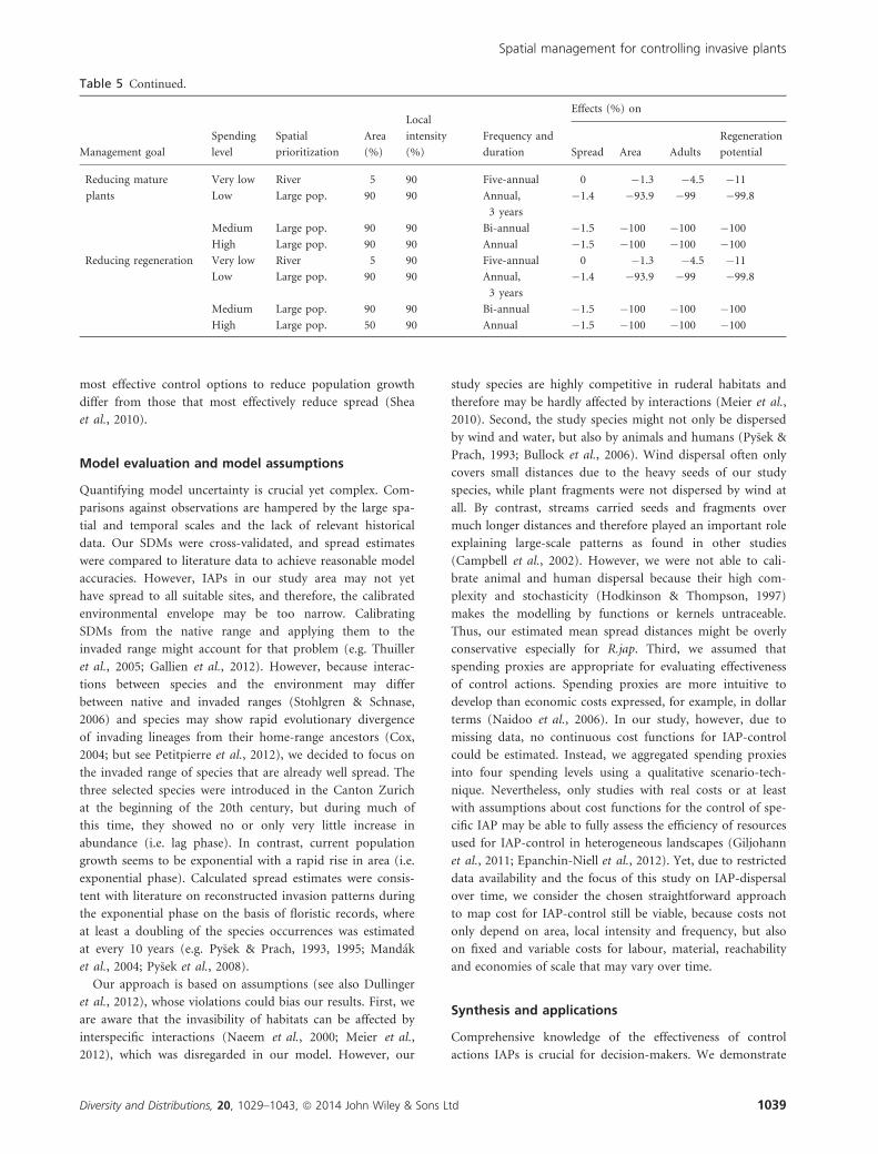
most effective control options to reduce population growth

differ from those that most effectively reduce spread (Shea

et al., 2010).

Model evaluation and model assumptions

Quantifying model uncertainty is crucial yet complex. Com-

parisons against observations are hampered by the large spa-

tial and temporal scales and the lack of relevant historical

data. Our SDMs were cross-validated, and spread estimates

were compared to literature data to achieve reasonable model

accuracies. However, IAPs in our study area may not yet

have spread to all suitable sites, and therefore, the calibrated

environmental envelope may be too narrow. Calibrating

SDMs from the native range and applying them to the

invaded range might account for that problem (e.g. Thuiller

et al., 2005; Gallien et al., 2012). However, because interac-

tions between species and the environment may differ

between native and invaded ranges (Stohlgren & Schnase,

2006) and species may show rapid evolutionary divergence

of invading lineages from their home-range ancestors (Cox,

2004; but see Petitpierre et al., 2012), we decided to focus on

the invaded range of species that are already well spread. The

three selected species were introduced in the Canton Zurich

at the beginning of the 20th century, but during much of

this time, they showed no or only very little increase in

abundance (i.e. lag phase). In contrast, current population

growth seems to be exponential with a rapid rise in area (i.e.

exponential phase). Calculated spread estimates were consis-

tent with literature on reconstructed invasion patterns during

the exponential phase on the basis of floristic records, where

at least a doubling of the species occurrences was estimated

at every 10 years (e.g. Py�sek & Prach, 1993, 1995; Mand�ak

et al., 2004; Py�sek et al., 2008).

Our approach is based on assumptions (see also Dullinger

et al., 2012), whose violations could bias our results. First, we

are aware that the invasibility of habitats can be affected by

interspecific interactions (Naeem et al., 2000; Meier et al.,

2012), which was disregarded in our model. However, our

study species are highly competitive in ruderal habitats and

therefore may be hardly affected by interactions (Meier et al.,

2010). Second, the study species might not only be dispersed

by wind and water, but also by animals and humans (Py�sek &

Prach, 1993; Bullock et al., 2006). Wind dispersal often only

covers small distances due to the heavy seeds of our study

species, while plant fragments were not dispersed by wind at

all. By contrast, streams carried seeds and fragments over

much longer distances and therefore played an important role

explaining large-scale patterns as found in other studies

(Campbell et al., 2002). However, we were not able to cali-

brate animal and human dispersal because their high com-

plexity and stochasticity (Hodkinson & Thompson, 1997)

makes the modelling by functions or kernels untraceable.

Thus, our estimated mean spread distances might be overly

conservative especially for R.jap. Third, we assumed that

spending proxies are appropriate for evaluating effectiveness

of control actions. Spending proxies are more intuitive to

develop than economic costs expressed, for example, in dollar

terms (Naidoo et al., 2006). In our study, however, due to

missing data, no continuous cost functions for IAP-control

could be estimated. Instead, we aggregated spending proxies

into four spending levels using a qualitative scenario-tech-

nique. Nevertheless, only studies with real costs or at least

with assumptions about cost functions for the control of spe-

cific IAP may be able to fully assess the efficiency of resources

used for IAP-control in heterogeneous landscapes (Giljohann

et al., 2011; Epanchin-Niell et al., 2012). Yet, due to restricted

data availability and the focus of this study on IAP-dispersal

over time, we consider the chosen straightforward approach

to map cost for IAP-control still be viable, because costs not

only depend on area, local intensity and frequency, but also

on fixed and variable costs for labour, material, reachability

and economies of scale that may vary over time.

Synthesis and applications

Comprehensive knowledge of the effectiveness of control

actions IAPs is crucial for decision-makers. We demonstrate

Table 5 Continued.

Management goal

Spending

level

Spatial

prioritization

Area

(%)

Local

intensity

(%)

Frequency and

duration

Effects (%) on

Spread Area Adults

Regeneration

potential

Reducing mature

plants

Very low River 5 90 Five-annual 0 �1.3 �4.5 �11


3 years

�1.4 �93.9 �99 �99.8



Reducing regeneration Very low River 5 90 Five-annual 0 �1.3 �4.5 �11


3 years

�1.4 �93.9 �99 �99.8





that taking a landscape-scale perspective on IAP-control sig-

nificantly enhances the effectiveness of control. Specifically,

our simulations peak in four recommendations: (i) IAP-

management planning should set spatial priorities of control

at a landscape level. Yet, spatial priorities must account for

specific landscape characteristics (e.g. the configuration of

suitable habitats), the stage of invasion and species traits,

because there is no one-fits-all control option that ensures

most effective control for all species and landscapes. (ii) Spa-

tial prioritization of IAP-control is particularly important

under budget restrictions. (iii) A careful selection of IAP-

control options is crucial, because spread of invading species

can be increased by ineffective control compared with doing

nothing. (iv) Given the same overall input of resources,

cumulative early control is more promising than intervening

bit by bit.

From a practical view point, optimal control options may

not be equally easy to implement. For instance, one may

provide practitioners with maps for controlling species in

highly connected habitats or along reaches of rivers. Advising

them to focus on small or large populations is much more

complex, because population sizes are highly volatile and

hence may not easily be mapped. This calls, however, for

both sound monitoring to assist management planning and

early treatment ascertaining rapid success.

Finally, the hybrid modelling approach used in this study

may substantially improve IAP-management planning at a

strategic level. Our modelling approach allows combining

IAP monitoring with an integrated tool for evaluating past,

present and planned future actions for IAP-control. In com-

bination with more detailed data on costs for IAP-control,

the modelling approach presented in this paper may help to

spend sparse financial resources in more efficient ways than

based exclusively on currently used bioeconomic optimiza-

tion models.

ACKNOWLEDGEMENTS

We thank T W€ust for technical assistance, Canton Zurich

(AWEL, Biosecurity) for access to cantonal databases, the EU

FP6 Grant GOCE-CT-2007-036866 (ECOCHANGE) for

funding and the Swiss Multi-Science Computing Grid

(SMSCG) for providing parts of the computing resources.

REFERENCES

Andersen, U.V. (1994) Sheep grazing as a method of control-

ling Heracleum mantegazzianum. Ecology and management

of invasive riverside plants (ed. by L.C. Waal, L.E. Child,

P.M. Wade and J.H. Brock), 217 p. Wiley, Chichester.

Andrew, M.E. & Ustin, S.L. (2010) The effects of temporally

variable dispersal and landscape structure on invasive spe-

cies spread. Ecological Applications, 20, 593–608.

ARE (2001) Kantonaler Richtplan (ed. Amt f€ur Raumord-

nung und Vermessung Kanton Z€urich).

AWEL (2007) €Okomorphologische Erhebung der Fliess-

gew€asser im Kanton Z€urich (ed. Amt f€ur Abfall Wasser

Energie und Luft AWEL).

AWEL (2008) Kieskataster des Kantons Z€urich (ed. Amt f€ur

Abfall Wasser Energie und Luft AWEL).

AWEL (2010) Neophytenkataster des Kantons Z€urich (ed.

Amt f€ur Abfall Wasser Energie und Luft AWEL) http://

www.gis.zh.ch/dokus/awel/abfallwirtschaft/neophyten.html

Beerling, D.J. & Perrins, J.M. (1993) Impatiens glandulifera

Royle (Impatiens roylei Walp.). Journal of Ecology, 81, 367–

382.

Besanko, D., Dranove, D., Shanley, M. & Schaefer, S. (2004)

Economics of strategy, 3rd edn. Wiley, New York, Chiches-

ter.

BFS & GEOSTAT (2000) BEK200 - Digitale Bodeneignungsk-

arte der Schweiz.

Bini, L.M., Diniz, J.A.F., Rangel, T. et al. (2009) Coefficient

shifts in geographical ecology: an empirical evaluation of

spatial and non-spatial regression. Ecography, 32, 193–204.

Blackwood, J., Hastings, A. & Costello, C. (2010) Cost-effec-

tive management of invasive species using linear-quadratic

control. Ecological Economics, 69, 519–527.

Borcard, D., Legendre, P. & Drapeau, P. (1992) Partialling

out the spatial component of ecological variation. Ecology,

73, 1045–1055.

Bossenbroek, J.M., Kraft, C.E. & Nekola, J.C. (2001) Predic-

tion of long-distance dispersal using gravity models: Zebra

mussel invasion of inland lakes. Ecological Applications, 11,

1778–1788.

Brabec, J. & Py�sek, P. (2000) Establishment and survival of

three invasive taxa of the genus Reynoutria (Polygonaceae)

in mesic mown meadows: a field experimental study. Folia

Geobotanica, 35, 27–42.

Bullock, J., Shea, K. & Skarpaas, O. (2006) Measuring plant

dispersal: an introduction to field methods and experimen-

tal design. Plant Ecology, 186, 217–234.

Burnham, K.P. & Anderson, D.R. (2002) Model selection and

multimodel inference: a practical information-theoretic

approach, 2nd edn. Springer, New York.

Campbell, G.S., Blackwell, P.G. & Woodward, F.I. (2002)

Can landscape-scale characteristics be used to predict plant

invasions along rivers? Journal of Biogeography, 29, 535–

543.

Cox, G.W. (2004) Alien species and evolution: the evolutionary

ecology of exotic plants, animals, microbes, and interacting

native species. Island Press, Washington, DC.

Damschen, E.I., Brudvig, L.A., Haddad, N.M., Levey, D.J.,

Orrock, J.L. & Tewksbury, J.J. (2008) The movement ecol-

ogy and dynamics of plant communities in fragmented

landscapes. Proceedings of the National Academy of Sciences

USA, 105, 19078–19083.

De Micheli, A., Bollens, U., Gelpke, G., Streit, B. & Fischer,

D. (2006) Bericht und Empfehlung zur Bek€ampfung des Jap-

ankn€oterichs. Kantone Aargau, Bern, Glarus, Luzern, Wallis

und Z€urich.


E. S. Meier et al.

Dormann, C.F., McPherson, J.M., Ara�ujo, M.B., Bivand, R.,

Bolliger, J., Carl, G., Davies, R.G., Hirzel, A., Jetz, W., Kis-

sling, W.D., K€uhn, I., Ohlem€uller, R., Peres-Neto, P.R.,

Reineking, B., Schr€oder, B., Schurr, F.M. & Wilson, R.

(2007) Methods to account for spatial autocorrelation in

the analysis of species distributional data: a review. Ecogra-

phy, 30, 609–628.

Dray, S. (2008) SpacemakeR: spatial modelling. R package

version 0.0-3. Available at: http://cran.r-project.org

Dullinger, S., Kleinbauer, I., Peterseil, J., Smolik, M. & Essl,

F. (2009) Niche based distribution modelling of an invasive

alien plant: effects of population status, propagule pressure

and invasion history. Biological Invasions, 11, 2401–2414.

Dullinger, S., Gattringer, A., Thuiller, W. et al. (2012)

Extinction debt of high-mountain plants under twenty-

first-century climate change. Nature Climate Change, 2,

619–622.

EEA/SEBI (2010) Number of the listed ‘worst’ terrestrial and

freshwater invasive alien species threatening biodiversity in

Europe. European Environment Agency, Expert Group on

trends in invasive alien species.

Epanchin-Niell, R.S. & Hastings, A. (2010) Controlling estab-

lished invaders: integrating economics and spread dynam-

ics to determine optimal management. Ecology Letters, 13,

528–541.

Epanchin-Niell, R.S., Haight, R.G., Berec, L., Kean, J.M. &

Liebhold, A.M. (2012) Optimal surveillance and eradica-

tion of invasive species in heterogeneous landscapes. Ecol-

ogy Letters, 15, 803–812.

Flather, C.H. & Bevers, M. (2002) Patchy reaction-diffusion

and population abundance: the relative importance of hab-

itat amount and arrangement. The American Naturalist,

159, 40–56.

Gallien, L., Douzet, R., Pratte, S., Zimmermann, N.E. & Thu-

iller, W. (2012) Invasive species distribution models – how

violating the equilibrium assumption can create new

insights. Global Ecology and Biogeography, 21, 1126–1136.

Giljohann, K.M., Hauser, C.E., Williams, N.S.G. & Moore,

J.L. (2011) Optimizing invasive species control across

space: willow invasion management in the Australian Alps.

Journal of Applied Ecology, 48, 1286–1294.

Groves, J.H., Williams, D.G., Caley, P., Norris, R.H. & Cait-

cheon, G. (2009) Modelling of floating seed dispersal in a

fluvial environment. River Research and Applications, 25,

582–592.

Guisan, A. & Zimmermann, N.E. (2000) Predictive habitat

distribution models in ecology. Ecological Modelling, 135,

147–186.

Hauser, C.E. & McCarthy, M.A. (2009) Streamlining ‘search

and destroy’: cost-effective surveillance for invasive species

management. Ecology Letters, 12, 683–692.

Higgins, S.I., Richardson, D.M. & Cowling, R.M. (2000)

Using a dynamic landscape model for planning the man-

agement of alien plant invasions. Ecological Applications,

10, 1833–1848.

Hijmans, R.J., Cameron, S.E., Parra, J.L., Jones, P.G. & Jarvis,

A. (2005) Very high resolution interpolated climate sur-

faces for global land areas. International Journal of Clima-

tology, 25, 1965–1978.

Hodkinson, D.J. & Thompson, K. (1997) Plant dispersal: the

role of man. Journal of Applied Ecology, 34, 1484–1496.

Hulme, P.E. (2003) Biological invasions: winning the science

battles but losing the conservation war? Oryx, 37, 178–193.

Hulme, P.E. (2006) Beyond control: wider implications for

the management of biological invasions. Journal of Applied

Ecology, 43, 835–847.

Ib�a~nez, I., Silander, J.A., Allen, J.M., Treanor, S.A. & Wilson,

A. (2009) Identifying hotspots for plant invasions and fore-

casting focal points of further spread. Journal of Applied

Ecology, 46, 1219–1228.

Katul, G.G., Porporato, A., Nathan, R., Siqueira, M., Soons,

M.B., Poggi, D., Horn, H.S. & Levin, S.A. (2005) Mecha-

nistic analytical models for long-distance seed dispersal by

wind. The American Naturalist, 166, 368–381.

Keller, R.P., Lodge, D.M., Lewis, M.A. & Shogren, J.F. (2009)

Bioeconomics of invasive species: integrating ecology, econom-

ics, policy, and management. Oxford University Press,

Oxford, UK.

Kot, M., Lewis, M.A. & van den Driessche, P. (1996) Dis-

persal data and the spread of invading organisms. Ecology,

77, 2027–2042.

Krug, R.M., Roura-Pascual, N. & Richardson, D.M. (2010)

Clearing of invasive alien plants under different budget sce-

narios: using a simulation model to test efficiency. Biologi-

cal Invasions, 12, 4099–4112.

Mack, R.N., Simberloff, D., Lonsdale, W.M., Evans, H.,

Clout, M. & Bazzaz, F.A. (2000) Biotic invasions: causes,

epidemiology, global consequences, and control. Ecological

Applications, 10, 689–710.

Mand�ak, B., Py�sek, P. & B�ımov�a, K. (2004) History of the

invasion and distribution of Reynoutria taxa in the Czech

Republic: a hybrid spreading faster than its parents. Preslia,

76, 15–64.

Marchetto, K.M., Jongejans, E., Shea, K. & Isard, S.A. (2010)

Plant spatial arrangement affects projected invasion speeds

of two invasive thistles. Oikos, 119, 1462–1468.

Masters, R.A. & Sheley, R.L. (2001) Principles and practices

for managing rangeland invasive plants. Journal of Range

Management, 54, 502–517.

McGarigal, K., Cushman, S.A., Neel, M.C. & Ene, E. (2002)

FRAGSTATS v3: spatial pattern analysis program for cate-

gorical maps. Computer software program produced by the

authors at the University of Massachusetts, Amherst.

Meier, E.S., Kienast, F., Pearman, P.B., Svenning, J.-C., Thu-

iller, W., Ara�ujo, M.B., Guisan, A. & Zimmermann, N.E.

(2010) Biotic and abiotic variables show little redundancy

in explaining tree species distributions. Ecography, 33,

1038–1048.

Meier, E.S., Lischke, H., Schmatz, D.R. & Zimmermann,

N.E. (2012) Climate, competition and connectivity affect



future migration and ranges of European trees. Global Ecol-

ogy and Biogeography, 21, 164–178.

Moody, M.E. & Mack, R.N. (1988) Controlling the spread of

plant invasions: the importance of nascent foci. Journal of

Applied Ecology, 25, 1009–1021.

Naeem, S., Knops, J.M.H., Tilman, D., Howe, K.M., Ken-

nedy, T. & Gale, S. (2000) Plant diversity increases resis-

tance to invasion in the absence of covarying extrinsic

factors. Oikos, 91, 97–108.

Naidoo, R., Balmford, A., Ferraro, P.J., Polasky, S., Ricketts,

T.H. & Rouget, M. (2006) Integrating economic costs into

conservation planning. Trends in Ecology & Evolution, 21,

681–687.

Neter, J., Wasserman, W. & Kutner, M.H. (1983) Applied lin-

ear regression models p. 547. Richard D. Irwin Inc., Home-

wood.

Nobis, M.P., Jaeger, J.A.G. & Zimmermann, N.E. (2009)

Neophyte species richness at the landscape scale under

urban sprawl and climate warming. Diversity and Distribu-

tions, 15, 928–939.

Petitpierre, B., Kueffer, C., Broennimann, O., Randin, C.,

Daehler, C. & Guisan, A. (2012) Climatic Niche shifts are

rare among terrestrial plant invaders. Science, 335, 1344–

1348.

Py�sek, P. & Prach, K. (1993) Plant invasions and the role of

riparian habiats: a comparison of four species alien to

central Europe. Journal of Biogeography, 20, 413–420.

Py�sek, P. & Prach, K. (1995) Invasion dynamics of Impatiens

glandulifera – A century of spreading reconstructed. Biolog-

ical Conservation, 74, 41–48.

Py�sek, P., Jaro�sik, V., M€ullerov�a, J., Pergl, J. & Wild,

J. (2008) Comparing the rate of invasion by Heracleum

mantegazzianum at continental, regional, and local scales.

Diversity and Distributions, 14, 355–363.

R Development Core Team (2011) R: a language and envi-

ronment for statistical computing. R Foundation for Statisti-

cal Computing, Vienna, Austria.

Ramula, S., Knight, T.M., Burns, J.H. & Buckley, Y.M. (2008)

General guidelines for invasive plant management based on

comparative demography of invasive and native plant popu-

lations. Journal of Applied Ecology, 45, 1124–1133.

Regan, T.J., McCarthy, M.A., Baxter, P.W.J., Panetta, F.D. &

Possingham, H.P. (2006) Optimal eradication: when to stop

looking for an invasive plant. Ecology Letters, 9, 759–766.

Richter, R., Dullinger, S., Essl, F., Leitner, M. & Vogl, G.

(2013a) How to account for habitat suitability in weed

management programmes? Biological invasions, 15, 657–

669.

Richter, R., Berger, U.E., Dullinger, S., Essl, F., Leitner, M.,

Smith, M. & Vogl, G. (2013b) Spread of invasive ragweed:

climate change, management and how to reduce allergy

costs. Journal of Applied Ecology, 50, 1422–1430.

Shea, K. & Kelly, D. (2004) Modeling for management of

invasive species: Musk thistle (Carduus nutans) in New

Zealand. Weed Technology, 18, 1338–1341.

Shea, K., Jongejans, E., Skarpaas, O., Kelly, D. & Sheppard,

A.W. (2010) Optimal management strategies to control

local population growth or population spread may not be

the same. Ecological Applications, 20, 1148–1161.

Smolik, M.G., Dullinger, S., Essl, F., Kleinbauer, I., Leitner,

M., Peterseil, J., Stadler, L.M. & Vogl, G. (2010) Integrating

species distribution models and interacting particle systems

to predict the spread of an invasive alien plant. Journal of

Biogeography, 37, 411–422.

Solow, A., Seymour, A., Beet, A. & Harris, S. (2008) The

untamed shrew: on the termination of an eradication pro-

gramme for an introduced species. Journal of Applied Ecol-

ogy, 45, 424–427.

Stohlgren, T.J. & Schnase, J.L. (2006) Risk analysis for

biological hazards: what we need to know about invasive

species. Risk Analysis, 26, 163–173.

Swisstopo (2003) DHM25 – Das digitale H€ohenmodell der

Schweiz.

Swisstopo (2008) VECTOR25 – Digitales Landschaftsmodell

der Schweiz.

Taylor, C.M. & Hastings, A. (2004) Finding optimal control

strategies for invasive species: a density-structured model for

Spartina alterniflora. Journal of Applied Ecology, 41, 1049–1057.

Thuiller, W., Richardson, D.M., Py�sek, P., Midgley, G.F.,

Hughes, G.O. & Rouget, M. (2005) Niche-based modelling

as a tool for predicting the risk of alien plant invasions at

a global scale. Global Change Biology, 11, 2234–2250.

Turner, M.G. (1989) Landscape ecology: the effect of pattern

on process. Annual Review of Ecology and Systematics, 20,

171–197.

Vil�a, M., Espinar, J.L., Hejda, M., Hulme, P.E., Jaro�s�ık, V.,

Maron, J.L., Pergl, J., Schaffner, U., Sun, Y. & Py�sek, P.

(2011) Ecological impacts of invasive alien plants: a

meta-analysis of their effects on species, communities and

ecosystems. Ecology Letters, 14, 702–708.

Wadsworth, R.A., Collingham, Y.C., Willis, S.G., Huntley,

B. & Hulme, P.E. (2000) Simulating the spread and man-

agement of alien riparian weeds: are they out of control?

Journal of Applied Ecology, 37, 28–38.

Wilson, J.R.U., Gairifo, C., Gibson, M.R. et al. (2011) Risk

assessment, eradication, and biological control: global

efforts to limit Australian acacia invasions. Diversity and

Distributions, 17, 1030–1046.

With, K.A. (2002) The landscape ecology of invasive spread.

Conservation Biology, 16, 1192–1203.

SUPPORTING INFORMATION

Additional Supporting Information may be found in the

online version of this article:

Table S1 Traits of Heracleum mantegazzianum, Impatiens

glandulifera and Reynoutria japonica.

Table S2 Overview of colonization estimates of suitable

habitats.


E. S. Meier et al.

Table S3 Overview of most effective management options

per species, spending level and management goal, compared

to most effective random management options.

Figure S1 Achieved effects for reducing spread, area, adults

and regeneration potential and required spending over

15 years of management.

BIOSKETCH

Eliane S. Meier is an ecologist at Agroscope Institute for

Sustainability Sciences ISS. Her research focuses on the

impact of local processes, such as species interactions, dis-

persal and landscape management, on the distribution of

species and biodiversity patterns in agricultural landscapes,

alpine and riparian ecosystems and forests.

Author contributions: E.S.M., D.B. and N.E.Z. designed the

research; E.S.M., K.H. and A.G. prepared and analysed the

data; E.S.M., S.D., K.H., N.E.Z. and D.B. wrote the paper.

Editor: Ingolf K€uhn



space matters when defining effective management for ... · space matters when deﬁning effective...

Documents