sovereign risk modelling and applications clément ménassé, vu-lan nguyen, christophe poquet, maud...
TRANSCRIPT

HAL Id: tel-01405437https://tel.archives-ouvertes.fr/tel-01405437
Submitted on 29 Nov 2016
HAL is a multi-disciplinary open accessarchive for the deposit and dissemination of sci-entific research documents, whether they are pub-lished or not. The documents may come fromteaching and research institutions in France orabroad, or from public or private research centers.
L’archive ouverte pluridisciplinaire HAL, estdestinée au dépôt et à la diffusion de documentsscientifiques de niveau recherche, publiés ou non,émanant des établissements d’enseignement et derecherche français ou étrangers, des laboratoirespublics ou privés.
Sovereign risk modelling and applicationsJean-Francois, Shanqiu Li
To cite this version:Jean-Francois, Shanqiu Li. Sovereign risk modelling and applications. Probability [math.PR]. Uni-versité Pierre et Marie Curie - Paris VI, 2016. English. <NNT : 2016PA066422>. <tel-01405437>

Université Pierre et Marie Curie - Paris VIUFR de Mathématiques
Thèsepour obtenir le grade de
Docteur de l’Université Paris 6Spécialité : Mathématiques Appliquées
présentée par
Shanqiu LI
Modélisation des risques souverains et applicationsSovereign risk modelling and applications
Co-dirigée par Pr. Ying JIAO et Pr. Huyên PHAM
Soutenue publiquement le 17 novembre 2016, devant le jurycomposé de :
Stéphane Crépey Rapporteur
Caroline Hillairet Examinatrice
Monique Jeanblanc Examinatrice
Ying Jiao Directrice de thèse
Idris Kharroubi Examinateur
Gilles Pagès Président du jury
Huyên Pham Directeur de thèse

LPMA - Université Paris DiderotBâtiment Sophie Germain, 5ème étage8, place Aurélie Nemours75205 PARIS CEDEX 13FRANCECase courrier 7012
LPMA - UPMCCouloir 16 - 26, 1er étage4, place Jussieu75252 PARIS CEDEX 05FRANCECase courrier 188

À ma famille


Remerciements
Je tiens tout d’abord à exprimer ma plus profonde gratitude à mes directeurs de thèseYing Jiao et Huyên Pham pour m’avoir guidé dans l’univers de la recherche scientifique.Je remercie Ying Jiao pour une colaboration passionnante et fructueuse avec la rigueurindispensable. Je suis également reconnaissant à Huyên Pham pour ses investissementsd’énergie et bon nombre de ses conseils.
Toute ma reconnaissance va également à Gilles Pagès et Francis Comets pour m’avoiraccueilli à bras ouverts au sein du LPMA, ainsi que Pascal Chiettini, Nathalie Bergameet Valérie Juvé pour leur services au niveau de l’administration.
Je souhaite aussi remercier Tomasz R. Bielecki, François Buet-Golfouse, StéphaneCrépey, Nicole El Karoui, Monique Jeanblanc, Shiqi Song et Thorsten Schmidt pourleurs disscusions et leurs remarques très précieuses, ainsi que Caroline Hillairet et IdrisKharroubi pour avoir accepté de faire partie du jury.
Ce fut un réel plaisir d’avoir travaillé au bâtiment Sophie Germain Université Paris Di-derot dans l’équipe Mathématiques financières et Probabilités numériques dont je remercietous les enseignants chercheurs : Laure Elie, Huyên Pham, Marie-Claire Quenez, PeterTankov, Jean-François Chassagneux, Simone Scotti, Noufel Frikha, Claudio Fontana, Zo-rana Grbac, ainsi que des post-doctorants et des doctorants avec qui j’ai eu des échangeset des partages : Andrea Cosso, Tingting Zhang, Jiatu Cai, Xiaoli Wei, Guillaume Barra-quand, Anna Benhamou, Oriane Blondel, Ngoc Huy Chau, Sébastien Choukroun, SophieCoquan, Aser Corines, Pietro Fodra, Adrien Genin, Marc-Antoine Giuliani, Pierre Gruet,Lorick Huang, Côme Huré, Amine Ismail, David Krief, Nicolas Langrené, Arturo Leos

iv
Zamorategui, Clément Ménassé, Vu-Lan Nguyen, Christophe Poquet, Maud Thomas etThomas Vareschi.
Enfin, je remercie ma famille et mes amis pour leur supports inconditionnels.

Résumé
La présente thèse traite la modélisation mathématique des risques souverains et sesapplications.
Dans le premier chapitre, motivé par la crise de la dette souveraine de la zone euro, nousproposons un modèle de risque de défaut souverain. Ce modèle prend en compte aussibien le mouvement de la solvabilité souveraine que l’impact des événements politiquescritiques, en y additionnant un risque de crédit idiosyncratique. Nous nous intéressonsaux probabilités que le défaut survienne aux dates d’événements politiques critiques, pourlesquelles nous obtenons des formules analytiques dans un cadre markovien, où noustraitons minutieusement quelques particularités inhabituelles, entre autres le modèle CEVlorsque le paramètre d’élasticité β > 1. Nous déterminons de manière explicite le processuscompensateur du défaut et montrons que le processus d’intensité n’existe pas, ce quioppose notre modèle aux approches classiques.
Dans le deuxième chapitre, en examinant certains modèles hybrides issus de la lit-térature, nous considérons une classe de temps aléatoires dont la loi conditionnelle estdiscontinue et pour lesquels les hypothèses classiques du grossissement de filtrations nesont pas satisfaites. Nous étendons l’approche de densité à un cadre plus général, oùl’hypothèse de Jacod s’assouplit, afin de traiter de tels temps aléatoires dans l’universdu grossissement progressif de filtrations. Nous étudions également des problèmes clas-siques : le calcul du compensateur, la décomposition de la surmartingale d’Azéma, ainsique la caractérisation des martingales. La décomposition des martingales et des semimar-tingales dans la filtration élargie affirme que l’hypothèse H’ demeure valable dans ce cadregénéralisé.

vi
Dans le troisième chapitre, nous présentons des applications des modèles proposés dansles chapitres précédents. L’application la plus importante du modèle de défaut souverain etde l’approche de densité généralisée est l’évaluation des titres soumis au risque de défaut.Les résultats expliquent les sauts négatifs importants dans le rendement actuariel del’obligation à long terme de la Grèce pendant la crise de la dette souveraine. La solvabilitéde la Grèce a tendance à s’empirer au fil des années et le rendement de l’obligation a dessauts négatifs lors des événements politiques critiques. En particulier, la taille d’un sautdépend de la gravité d’un choc exogène, du temps écoulé depuis le dernier événementpolitique, et de la valeur du recouvrement. L’approche de densité généralisée rend aussipossible la modélisation des défauts simultanés qui, bien que rares, ont un impact gravesur le marché.
Mots-clefs
Risque souverain, solvabilité souveraine, risque de crédit idiosyncratique, décomposi-tion de temps d’arrêt, hypothèse de densité généralisée, grossissement progressif de fil-trations, caractérisation de martingale, décomposition de semimartingale, propriété d’im-mersion, défauts simultanés, obligation souveraine à long terme.

Abstract
This dissertation deals with the mathematical modelling of sovereign credit risk andits applications.
In Chapter 1, motivated by the European sovereign debt crisis, we propose a hybridsovereign risk model which takes into account both the movement of the sovereign solvencyand the impact of critical political events besides the idiosyncratic credit risk. We areinterested in the probability that the default occurs at critical political dates, for whichwe obtain closed-form formulae in a Markovian setting, where we deal with some unusualfeatures, such as a treatment of the CEV model when the elasticity parameter β > 1.We compute explicitly the compensator process of default and show that the intensityprocess does not exist.
In Chapter 2, by studying certain hybrid models in literature on credit risks, weconsider a type of random times whose conditional probability distribution is not con-tinuous and by which standard intensity and density hypotheses in the enlargement offiltrations are not satisfied. We propose a generalised density approach, where the hy-pothesis of Jacod is relaxed, in order to deal with such random times in the framework ofprogressive enlargement of filtrations We also study classic problems such as the compu-tation of the compensator process of the random time, the decomposition of the Azémasupermartingale, as well as the martingale characterisation. The martingale and semi-martingale decompositions in the enlarged filtration show that the H’-hypothesis holds inthis generalised framework.
In Chapter 3, we display several applications of the models proposed in the previous

viii
chapters. The most important application of the hybrid default model and the generaliseddensity approach is the valuation of default claims. The results explain the significantnegative jumps in the long-term Greek government bond yield during the sovereign debtcrisis. The solvency of Greece tends to fall gradually through time and the bond yieldhas negative jumps when critical political events are held. In particular, the size of ajump depends on the seriousness of an exogenous shock, the elapsed time since the lastpolitical event, and the value of the recovery payment. The generalised density approachalso makes possible the modelling of simultaneous defaults, which are rare but may havean important impact.
Keywords
Sovereign risk, sovereign solvency, idiosyncratic credit risk, decomposition of stoppingtimes, generalised density hypothesis, progressive enlargement of filtrations, martingalecharacterisation, semimartingale decomposition, immersion property, simultaneous de-faults, long-term government bond.

Notations
Chapter 1
— (Ω,A,P) is a probability space equiped with a filtration F = (Ft)t≥0.— τ is the default time.— G = (Gt)t≥0 is the progressive enlargement of the filtration F by τ .— W = (Wt, t ≥ 0) is an F-adapted standard Brownian motion.— S = (St, t ≥ 0) is the solvency process of a sovereign.— τ0 is the first hitting time of the barrier L > 0 by the process S.— (τi)ni=1 is a sequence of first hitting times of the decreasing barrier sequence L1, . . . , Ln
by the process S.— ζ and ζ∗ are accessible stopping times, and ξ is a totally inaccessible stopping time.— N = (Nt, t ≥ 0) is a Poisson process.— λN is the constant Poisson intensity, and λN(t) is the time-dependent Poisson
intensity function.— λ = (λt, t ≥ 0) is the idiosyncratic default intensity process, and Λ = (Λt, t ≥ 0) =
(∫ t
0 λs ds, t ≥ 0).— η is an A-measurable random variable.— σ1 ∧ σ2 is the minimum of two random times σ1 and σ2.— pi = (pit, t ≥ 0) is the F-conditional probability that τ coincides with τi, i.e.,
pit = P(τ = τi|Ft), i ∈ 1, . . . , n.
— G = (Gt, t ≥ 0) is the Azéma F-supermartingale of τ .— ΛF = (ΛF
t , t ≥ 0) is the F-compensator process such that (1τ≤t − ΛFt∧τ , t ≥ 0) is a

x
G-martingale.— ΛG = (ΛG
t , t ≥ 0) is the G-compensator process such that ΛGt = ΛF
t∧τ .— Γ = (Γt, t ≥ 0) is the hazard process of τ such that Γt = − lnGt.— E(X) is the Doléans-Dade exponential of any process X.— L is the infinitesimal generator of a diffusion.— Iν(x) and Kν(x) are modified Bessel functions of the first and second kind.— Mn,m(x) and Wn,m(x) are Whittaker functions of the first kind and second kind.— F1(a, b, x) and F2(a, b, x) are Kummer confluent hypergeometric functions of the
first kind and second kind.
Chapter 2
— η is a non-atomic σ-finite Borel measure on R+.— B is Borel σ-algebra.— (Ω,A,F,P) is a filtered probability space where F = (Ft)t≥0 is the reference filtra-
tion satisfying the usual conditions.— O(F) and P(F) are the optional and predictable σ-algebra associated to the filtra-
tion F.— τ is an arbitrary random time which is not an F-stopping time.— G = (Gt)t≥0 is the enlargement of the filtration F by τ .— (τi)Ni=1 is a finite family of F-stopping times.— α(· · · ) = (αt(· · · ), t ≥ 0) is the generalised density process.— σ1 ∨ σ2 is the maximum of two random times σ1 and σ2.— Di = (Di
t, t ≥ 0) is the indicator process associated to τi, i.e., Dit = 1τi≤t,
i ∈ 1, . . . , N.— Λi = (Λi
t, t ≥ 0) is the compensator of Di such that M i = Di − Λi is an F-martingale, i ∈ 1, . . . , N.
— A = (At, t ≥ 0) is the F-dual predictable projection of the indicator process(1τ≤t, t ≥ 0).
Chapter 3

xi
— Q is an equivalent probability measure.— (rt, t ≥ 0) is default-free interest rate process.— (Rt, t ≥ 0) is the recovery paiement process.— D(t, T ) is the value of the defaultable zero-coupon bond.— Y d(t, T ) and Y (t, T ) are respectively the yield to maturity of the defaultable zero-
coupon bond and that of a classic default-free zero-coupon bond.— S(t, T ) is the credit spread of the defaultable zero-coupon bond.— κ is the CDS spread.

xii

Table des matières
Introduction générale en français 1
Introduction 13
1 A hybrid model for sovereign risk 25
1.1 Introduction . . . . . . . . . . . . . . . . . . . . . . . . . . . . . . . . . . . 26
1.2 Hybrid model of sovereign default time . . . . . . . . . . . . . . . . . . . . 31
1.2.1 Sovereign solvency: a structural model . . . . . . . . . . . . . . . . 32
1.2.2 Critical political event . . . . . . . . . . . . . . . . . . . . . . . . . 36
1.2.3 Idiosyncratic credit risk: a Cox process model . . . . . . . . . . . . 37
1.2.4 Sovereign default time: a hybrid model . . . . . . . . . . . . . . . . 38
1.2.5 Extension to re-adjusted solvency thresholds . . . . . . . . . . . . . 39
1.2.6 Immersion property under minimum . . . . . . . . . . . . . . . . . 42
1.3 Probability of default on multiple critical dates . . . . . . . . . . . . . . . 44
1.3.1 Conditional default and survival probabilities . . . . . . . . . . . . 44
1.3.2 Compensator process . . . . . . . . . . . . . . . . . . . . . . . . . . 46
1.3.3 Default probability in a Markovian setting . . . . . . . . . . . . . . 48
1.3.3.1 Case of geometric Brownian motion . . . . . . . . . . . . . 52

xiv Table des matières
1.3.3.2 Case of the CEV process . . . . . . . . . . . . . . . . . . . 54
1.3.4 Numerical illustrations . . . . . . . . . . . . . . . . . . . . . . . . . 58
1.4 Hybrid model beyond immersion paradigm . . . . . . . . . . . . . . . . . . 61
2 Generalised density approach for sovereign risk 67
2.1 Introduction . . . . . . . . . . . . . . . . . . . . . . . . . . . . . . . . . . . 68
2.2 Generalised density hypothesis . . . . . . . . . . . . . . . . . . . . . . . . . 71
2.2.1 Key assumption . . . . . . . . . . . . . . . . . . . . . . . . . . . . . 72
2.2.2 Examples in literature . . . . . . . . . . . . . . . . . . . . . . . . . 83
2.3 Compensator process . . . . . . . . . . . . . . . . . . . . . . . . . . . . . . 87
2.4 Sovereign default model revisited . . . . . . . . . . . . . . . . . . . . . . . 92
2.5 Martingales and semimartingales in G . . . . . . . . . . . . . . . . . . . . 93
3 Applications of sovereign default risk models in finance 101
3.1 Introduction . . . . . . . . . . . . . . . . . . . . . . . . . . . . . . . . . . . 102
3.2 Valuation of defaultable claims . . . . . . . . . . . . . . . . . . . . . . . . 103
3.2.1 Sovereign bond and credit spread . . . . . . . . . . . . . . . . . . . 103
3.2.2 Sovereign CDS . . . . . . . . . . . . . . . . . . . . . . . . . . . . . 107
3.2.3 Example of indifference pricing in a hybrid model . . . . . . . . . . 108
3.2.4 Numerical illustrations . . . . . . . . . . . . . . . . . . . . . . . . . 114
3.2.5 Pricing credit risk in generalised density framework . . . . . . . . . 116
3.3 A two-name model with simultaneous defaults . . . . . . . . . . . . . . . . 125
A Some classic results 129
B Some proofs 133

Table des matières xv
B.1 Proof of Proposition 2.13 . . . . . . . . . . . . . . . . . . . . . . . . . . . . 133
B.2 Proof of Theorem 3.2 . . . . . . . . . . . . . . . . . . . . . . . . . . . . . . 134
List of Figures 137
Bibliography 139


Introduction générale en français
Cette thèse traite la modélisation mathématique du risque souverain ainsi que sesapplications en finance. Ces études se basent sur la crise de la dette souveraine dans lazone euro, provoquée par la mise en lumière de la crise de la dette grecque, qui demeureun sujet d’actualité depuis fin 2009.
La crise de la dette dans la zone euro résulte d’importants déficits publics et des effetsde contagion financière. Plusieurs états membres de la zone euro (Grèce, Portugal, Irlande,Espagne, et Chypre) furent dans l’incapacité de rembourser ou de refinancer leurs dettespubliques sans intervention d’un tiers, tel que d’autres états membres de la zone euro, laBanque Centrale Européenne (BCE), et le Fond Monétaire International (FMI), etc.
Différent du risque de crédit d’entreprise, le risque souverain a des caractères mixtesdus à une combinaison de facteurs macroéconomiques et géopolitiques complexes, commec’est le cas pour un état membre de la zone euro. Des études empiriques suggèrent queles facteurs macroéconomiques déterminants peuvent être résumés par un facteur com-mun nommé solvabilité souveraine (voir e.g. Alogoskoufis [Alo12]), et les impacts desdécisions politiques surviennent notamment lors d’un événement politique critique fixéà l’avance. Ces impacts politiques sont caractérisés par une probabilité de défaut élevéeantérieurement à l’événement susmentionné, ainsi qu’une chute subite de cette probabilitéà la suite de celui-ci. Ce phénomène s’interprète par les équilibres multiples du marchéde dette en présence du risque de crédit et se visualise dans les variations importantesdu rendement actuariel des obligations souveraines. Précisément, du point de vue éco-nomique, l’équilibre dominant dépend des attentes des investisseurs sur la probabilitéde défaut (e.g., Calvo [Cal88]). Avant un événement politique critique, les investisseurs

2 Introduction générale en français
s’attendent à un défaut souverain avec une probabilité élevée, et le marché d’obligationssouveraines manifeste donc un équilibre de spread 1 large. Peu après cet événement, lesattentes des investisseurs sur le défaut souverain diminuent soudainement de sorte quele marché d’obligations d’état se trouve dans un équilibre de spread étroit. Pour cetteraison, la probabilité de défaut au moment de l’événement est non nulle, caractérisée parun saut dans le rendement actuariel.
Dans les modèles en temps continu, le temps de défaut est habituellement modélisécomme un temps aléatoire, et en particulier, un temps d’arrêt par rapport à une certainefiltration. En théorie de probabilité, les temps d’arrêt sont classifiés en trois catégories :temps d’arrêt prévisibles, accessibles, et totalement inaccessibles. Intuitivement, un tempsd’arrêt prévisible est connu juste avant l’arrivée d’un événement puisqu’il est annoncé parune suite croissante de temps d’arrêt ; un temps d’arrêt accessible peut être parfaitementcouvert par une suite de temps d’arrêt prévisibles ; et un temps d’arrêt totalement in-accessible est l’instant même d’une surprise totale qui ne coïncide jamais avec un tempsd’arrêt prévisible.
Dans la littérature sur les modélisations de risque de crédit, il existe déjà deux ap-proches classiques (voir les livres de Bielecki et Rutkowski [BR02], de Duffie et Singleton[DS03] et de Schönbucher [Sch03], et aussi les ouvrages de Bielecki, Jeanblanc et Rutkowski[BJR04b] et de Schmidt et Stute [SS03] pour une description détaillée) : l’approche struc-turelle (Black et Scholes [BS73], Merton [Mer74], Black et Cox [BC76]) où le temps dedéfaut est souvent un temps d’arrêt prévisible, et l’approche à forme réduite (aussi com-munément appelé approche d’intensité, Jarrow et Turnbull [JT92, JT95], Lando [Lan98],Duffie et Singleton [DS99]), où le temps de défaut est un temps d’arrêt totalement in-accessible. D’ailleurs, dans certains modèles structurels avec rapports de comptabilitéimparfaits (e.g., Duffie et Lando [DL01b], Giesecke [Gie06]), le temps de défaut est éga-lement totalement inaccessible. Récemment, Jarrow and Protter ([JP04]) montrent d’unpoint de vue informationnel que l’on peut transformer un temps d’arrêt en modifiantl’ensemble d’information à la disposition du modélisateur.
1. Spread est un anglicisme qui signifie l’écart entre le rendement actuariel d’une obligation et un tauxde référence.

Introduction générale en français 3
Pour l’analyse de risque de crédit, le grossissement progressif de filtrations (e.g., Bar-low, Jacod, Yor, et Jeulin [Bar78, Jac85, Jeu80, JY78, Yor78]) a été systématiquementadopté pour modéliser les événements de défaut qu’un modélisateur ne peut pas observerdu flux informationel du marché hors défaut, ou de manière mathématique, le temps dedéfaut n’est pas modélisé comme un temps d’arrêt par rapport à la filtration de réfé-rence (voir également Mansuy et Yor [MY06], Protter [Pro05], Dellacherie, Maisonneuveet Meyer [DMM92], Yor [Yor12], Brémaud et Yor [BY78], Nikeghbali [Nik06], Ankirchner[Ank05], Song [Son87], Ankirchner, Dereich et Imkeller [ADI07], Yœurp [Yœu85]). Dansles travaux de Elliott, Jeanblanc et Yor [EJY00] et de Bielecki et Rutkowski [BR02], lesauteurs ont proposé d’utiliser le grossissement progressif de filtrations pour décrire lesinformations du marché qui incluent tant l’information hors défaut que celle à l’égard dudéfaut. Précisément, les informations globales du marché sont modélisées comme la pluspetite filtration contenant toute l’information hors défaut telle que le temps de défaut estun temps d’arrêt. Plus récemment, afin d’étudier l’impact des événements de défaut, unenouvelle approche a été développée par El Karoui, Jeanblanc and Jiao [EKJJ10, EKJJ15]où l’on suppose l’hypothèse de densité. En particulier, l’approche de densité nous permetd’analyser ce qui arrive postérieurement à un événement de défaut et fait naître des ap-plications intéressantes dans les études de risque de défaut de contrepartie. Remarquonsque, dans l’approche d’intensité et l’approche de densité, le temps de défaut est un tempsd’arrêt totalement inaccessible.
La théorie de la décomposition de temps d’arrêt stipule que chaque temps d’arrêtpeut être décomposé de façon unique en une partie accessible et une autre totalementinaccessible (Dellacherie [Del72]). La décomposition de temps aléatoire apparaît égalementdans la littérature sur la théorie du grossissement de filtrations (e.g., Coculescu [Coc09],Aksamit, Choulli et Jeanblanc [ACJ16]). Pour le cas du défaut souverain, du point devue d’une telle décomposition, si le temps de défaut peut coïncider avec une date critiquearrêtée d’avance dont la probabilité est strictement positive, alors cela signifie que letemps de défaut possède une partie accessible outre qu’une partie totalement inaccessible.D’une part, ni l’approche à forme réduite ni l’approche de densité ne sont réalistes carle temps de défaut ainsi modélisé est totalement inaccessible et évite tous les temps

4 Introduction générale en français
d’arrêt prévisibles. D’autre part, un modèle structurel n’est pas adapté au défaut souveraincomme révèle Matsumura dans [Mat06], parce qu’il n’est pas clair quelle est la valeurd’actif à prendre pour référence et l’impact des décisions politiques ne se reflète pas surla définition structurelle dans la littérature. Pour cette raison, nous proposons un modèlehybride qui se base sur les deux approches classiques et en même temps prend en compteaussi bien le niveau de la solvabilité souveraine que l’impact des événements politiquescritiques.
Andreasen [And03] est l’un des premiers à étudier ce type de modèle hybride. Il existedans la littérature sur le risque de crédit d’autres modèles hybrides tels que le modèlegénéralisé à processus de Cox de Bélanger, Shreve et Wong [BSW04], le modèle hybridede migration de crédit de Chen et Filipović [CF05], les modèles CEV 2 de défaut ponctuelde Carr et Linetsky [CL06] et de Campi, Polbennikov et Sbuelz [CPS09], ainsi que le cadregénéral sans intensité de Gehmlich et Schmidt [GS16] et Fontana et Schmidt [FS16]. Plusprécisément, dans [BSW04], le processus de compensateur peut posséder des sauts ; dans[CF05], le défaut de la firme est provoqué soit par des dégradations successives de sa notede crédit, soit par un saut imprévisible d’un simple processus ponctuel ; dans [CL06], lavaleur d’action est une diffusion CEV ponctuée par un possible saut à zéro qui correspondà un défaut, et le temps de défaut est décomposé en une partie prévisible, qui est le premiertemps de passage à zéro par le processus de la valeur d’action, et une partie totalementinaccessible donnée par un modèle à processus de Cox ; dans [CPS09], la valeur d’actionest un processus CEV, et le temps de défaut est le minimum du premier instant de saut duprocessus de Poisson et le premier temps d’absorption du processus de la valeur d’actionpar zéro en l’absence de sauts ; dans [GS16], la surmartingale d’Azéma du temps de défautcontient des sauts de telle sorte que l’intensité n’existe pas, et [FS16] généralise l’approchede [GS16].
Dans le Chapitre 1, nous proposons un modèle hybride de défaut souverain où le tempsde défaut combine une partie accessible prenant en compte le mouvement de la solvabi-lité souveraine et l’impact des événements politiques critiques, et une partie totalementinaccessible pour le risque de crédit idiosyncratique. Les caractéristiques principales de
2. Modèles à élasticité de variance constante.

Introduction générale en français 5
notre modèle comprennent : le temps de défaut peut coïncider avec une famille de tempsd’arrêt prévisibles, la modélisation de l’impact des facteurs macroéconomiques et des évé-nements politiques est séparée de celle du risque idiosyncratique, la solvabilité peut êtrecorrélée avec le risque idiosyncratique, la propriété d’immersion est satisfaite et peut êtrefacilement relaxée.
Nous nous inspirons des modèles CEV de défaut ponctuel dans [CL06] et [CPS09],qui furent initialement proposés pour évaluer les risques de crédit d’entreprise. Ce quifait la différence, c’est que le défaut dans notre modèle peut coïncider avec de multiplesévénements politiques et peut arriver à la suite de n’importe lequel de ces événements,alors que le temps de défaut dans [CL06] et [CPS09] est borné par son seul composantprévisible.
La notion de solvabilité souveraine est importante dans notre modèle. la solvabilitéest une variable unifiée qui reflète l’impact des facteurs macroéconomiques sur la capa-cité d’un souverain de remplir ses obligations à long terme. Nous utilisons la définitionexistante de la solvabilité souveraine en temps discret ([Alo12]) à un modèle en tempscontinu et considérons un souverain (e.g., Grèce) avec processus de solvabilité (St, t ≥ 0),adapté par rapport à la filtration de référence F. Notre modèle est basé sur l’abstractionmathématique du scénario suivant : les autorités (BCE, Commission Européenne, FMI,etc.) établissent une condition de budget pour le souverain. Si le processus de solvabilité Stombe en-dessous du niveau requis, nous considérons que le souverain devient sévèrementinsolvable, et un événement politique critique doit être organisé, et lors de celui-ci desdécisions politiques doivent être prises à l’égard du souverain. Le résultat des décisionspeut être la faillite immédiate du souverain ou un plan d’aide financière pour celui-ci dansle but d’améliorer sa situation budgétaire. Dans ce dernier cas, si la situation aggravéede la dette et du déficit est excessive et ne permet pas d’amélioration satisfaisante, lesautorités peuvent relaxer la condition budgétaire et anticipent de nouveaux événementspolitiques critiques.
Le temps de défaut τ dans notre modèle se décompose de manière unique en une partieaccessible ζ∗ et une partie totalement inaccessible ξ sur une unique partition de l’ensemble

6 Introduction générale en français
d’échantillons Ω :τ(ω) = ζ∗(ω) ∧ ξ(ω).
La partie accessible ζ∗ est recouverte par une suite croissante de premiers temps de passage(F-temps d’arrêt) à n seuils de solvabilité τ1, . . . , τn :
τi = inft ≥ 0 : St < Li.
Le fait de savoir si le défaut coïncide ou non avec l’un des F-temps d’arrêt τi dépend d’unfacteur exogène (e.g., l’ampleur d’un choc financier externe qui précède τi), modélisé poursimplicité par un processus de Poisson inhomogène (Nt, t ≥ 0) avec fonction d’intensitéλN(t). La partie totalement inaccessible ξ admet un processus d’intensité (λt, t ≥ 0),qui peut être corrélé avec la solvabilité S. La structure globale d’information G est legrossissement progressif de la filtration F par le temps de défaut τ .
Nous calculons les probabilités que le défaut souverain ait lieu à des dates spécifiquesd’événements politiques critiques :
P(τ = τi|Ft) = E[(e−∫ τi−1
0 λN (s)ds − e−∫ τi
0 λN (s)ds)e−∫ τi
0 λs ds∣∣∣∣Ft] .
Tout comme ce que nous voudrions montrer, ces probabilités de défaut sont strictementpositives dans notre modèle hybride, ce qui implique la présence des singularités dans laloi du temps de défaut τ :
P(τ > u|Ft) = E[exp
(−
n∑i=1
1τi≤u∫ τi
τi−1λN(s)ds−
∫ u
0λs ds
)∣∣∣∣Ft].
Par conséquent, la surmartingale d’Azéma n’est pas continue à τ1, . . . , τn, et le processusde hasard 3 (∫ t
0λs ds+
n∑i=1
1τi≤t∫ τi
τi−1λN(s)ds, t ≥ 0
).
n’est pas égal au processus F-compensateur(∫ t
0λs ds+
n∑i=1
1τi≤t(
1− e−∫ τiτi−1
λN (s)ds), t ≥ 0
)
bien qu’ils aient la même partie continue.
3. La traduction littérale du terme en anglais hazard process.

Introduction générale en français 7
Dans un cadre markovien spécifique, où le processus de solvabilité et le processusde Poisson sont homogènes, les probabilités P(τ = τi|Ft) peuvent être déduites de latransformée de Laplace du temps d’arrêt ρ = inft ≥ 0 : St ≤ L :
E[exp
(−kρ−
∫ ρ
0λ(Su) du
)],
qui est la répresentation de la solution au problème de Dirichlet suivant
µ(z)u′(z) + 12σ
2(z)u′′(z) = (λ(z) + k)u(z) sur z > L;
u(L) = 1.
Nous obtenons les formules analytiques en résolvant des équations de Sturm-Liouvilledans les cas de mouvement brownien géométrique et de processus CEV. Plus précisément,quand le processus de solvabilité est modélisé par un mouvement brownien géométrique
dSt = St(µ dt+ σ dWt),
il s’agit des expressions en termes des solutions à une équation de Bessel modifée
(xy′)′ − c1x−1y′ = c2xy
où c1, c2 > 0, alors que dans le cas du processus de solvabilité modélisé par une diffusionCEV
dSt = St(µ dt+ δSβt dWt),
nous devons résoudre l’équation différentielle suivante
12δ
2x2+2βu′′ + µxu′ − (ax−2|β| + b+ k)u = 0,
où nous discutons le signe du paramètre d’élasticité β et obtenons les solutions fondamen-tales en employant les fonctions de Whittaker et les fonctions de Bessel modifiées.
La propriété d’immersion possède l’avantage d’impliquer la complétude du marché (e.g.[JLC09a]). Cependant, il est généralement impossible de supposer l’immersion dans lescas de marché incomplet, de multi-defauts non-ordonnés, et de corrélation entre différentstemps de défaut. Dans notre modèle hybride, la propriété d’immersion est controlée par la

8 Introduction générale en français
barrière aléatoire, ou plus précisément, la propriété d’immersion est satisfaite si la barièrealéatoire est indépendante de F∞. En relaxant l’hypothèse d’indépendance susmentionnée,nous pouvons étendre le modèle au delà du paradigme d’immersion. Par conséquent, lasurmartingale d’Azéma n’est plus un processus décroissant, et nous devons faire appel àla décomposition multiplicative pour obtenir le processus compensateur.
D’un point de vue probabiliste appuyé par notre calcul, les probabilités de défautnon nulle aux dates d’événements politiques critiques signifient que la loi du temps dedéfaut τ admet des singularités. Afin d’étendre notre modèle de risque souverain à uncadre plus général, nous considérons un type de temps aléatoires qui peuvent être soitaccessibles soit totalement inaccessibles et proposons de généraliser l’approche de densitédans [EKJJ10]. Plus précisément, nous supposons que la loi conditionnelle de τ contientune partie singulière outre que la partie absolument continue qui a une densité.
Dans le Chapitre 2, F = (Ft)t≥0 est la filtration de référence et G = (Gt)t≥0 est legrossissement progressif de F par τ , et nous supposons l’hypothèse de densité généraliséeque la loi F-conditionnelle de τ évitant une famille de F-temps d’arrêt (τi)ni=1 a une densité(nommée densité généralisée) par rapport à une mesure borélienne σ-finie non-atomiqueη sur R+ :
E[1Hh(τ) | Ft] =∫R+h(u)αt(u) η(du) P-p.s.,
où H désigne l’ensemble aléatoire
τ <∞ ∩n⋂i=1τ 6= τi.
Notre hypothèse clef est satisfaite par d’autres modèles hybrides précédemment cités telsque [BSW04, CF05, CL06, CPS09, GS16], ainsi que notre modèle de risque souverain duChapitre 1 dans les deux versions avec et sans propriété d’immersion, et nous pouvonsexpliciter le processus de densité généralisée pour chacun de ces modèles. Sous l’hypothèsede densité généralisée, τ n’a que la possibilité de rencontrer les F-temps d’arrêt qui peuventcoïncider avec (τi)ni=1. Nous prouvons que le processus de densité généralisée α(·) est uneF-martingale càdlàg paramétrée. Notons (pit, t ≥ 0) les probabilités F-conditionnelle queτ rencontre τi, i ∈ 1, . . . , n, alors toute espérance Gt-conditionnelle peut être calculéesous la forme décomposée en termes de α(·) et (pi)ni=1. En outre, nous pouvons montrer

Introduction générale en français 9
que la formule de décomposition suivante pour les processus G-optionnels est valable, cequi n’est pas le cas en général
Y Gt = 1τ>tYt + 1τ≤tYt(τ), P-p.s.
La validité de la formule ci-dessus a été vérifiée à maintes reprises pour les modèlesexistants, entre autres sous l’hypothèse de densité, et on peut en trouver les conditionsdans Song [Son14].
Le processus compensateur sous l’hypothèse de densité généralisée n’est pas en généralun processus continu et donc le processus d’intensité n’existe pas toujours. Nous traitonsla décomposition de Doob-Meyer de la surmartingale d’Azéma G et nous nous concentronssur sa partie discontinue afin d’obtenir la forme générale du compensateur
ΛGt =
∫ t∧τ
01Gs−>0
αs(s)η(ds)Gs−
+n∑i=1
∫(0,t∧τ ]
1Gs−>0pis−dΛi
s + d〈M i, pi〉sGs−
, t ≥ 0,
où Λi = (Λit, t ≥ 0) est le compensateur de (1τi≤t, t ≥ 0) et
M i =(1τi≤t − Λi
t, t ≥ 0)
pour tout i = 1, . . . , n. Si (τi)ni=1 sont des F-temps d’arrêt prévisibles, alors τ est unG-temps d’arrêt accessible et le processus de compensateur de τ possède une partie ab-solument continue et une partie avec des sauts à (τi)ni=1 ; s’ils sont par ailleurs F-tempsd’arrêt totalement inaccessibles, alors τ est un G-temps d’arrêt totalement inaccessible etle processus compensateur de τ est continu.
Nous caractérisons également les martingales dans la filtration G en vérifiant troisconditions sur des F-martingales. Différent de [EKJJ10], les conditions nécessaires et lesconditions suffisantes sont subtilement distinguées. La stabilité des semimartingales estaussi un problème classique à étudier quand la filtration de référence est élargie. Nousobtenons la décomposition d’une F-martingale locale en tant que G-semimartingale
UFt = UG
t +∫
(0,t∧τ ]
d〈UF, M〉sGs−
+ 1∩Ni=1τ 6=τi
∫(τ,t∨τ ]
d〈UF, α(u)〉sαs−(u)
∣∣∣∣u=τ
+n∑i=1
1τ=τi
∫(τ,t∨τ ]
d〈UF, pi〉spis−
,

10 Introduction générale en français
où UG est une G-martingale locale et M est une F-martingale BMO, calculée par
Mt = E[∫ ∞
0αu(u)η(du)
∣∣∣∣Ft]+n∑i=1
pit∧τi + p∞t , t ≥ 0,
qui est en général différente de celle dans la décompostion de Doob-Meyer de G. Laformule de décomposition ci-dessus signifie que l’hypothèse (H’) de Jacod est satisfaitesous l’hypothèse de densité généralisée.
Dans le Chapitre 3, nous appliquons les résultats des chapitres précédents à l’évaluationet à la couverture des risques de crédit. L’une des applications les plus importantes dumodèle de risque souverain est l’évaluation des titres soumis au risque souverain tels queles obligations souveraines. Nous nous intéressons particulièrement au comportement durendement actuariel à long terme durant la crise de la dette souveraine, et nous montronsque le modèle hybride fournit une interprétation au comportement des sauts autour desdates d’événements politiques critiques. Précisément, le saut dans la valeur d’obligationD(t, T ) à la date τi est caractérisé en termes du montant de recouvrement et du processusF-compensateur, donné par la formule suivante
∆D(τi, T ) = (D(τi, T )−Rτi)ΛFτi
on τi < T.
Le spread de crédit se comporte dans le sens inverse du prix d’obligation, qui est en généralplus élevé que le recouvrement, il est donc vraisemblable que le spread de crédit ait dessauts négatifs.
Nous donnons un exemple de valorisation à l’aide de l’optimisation de portefeuilledans un modèle hybride, où un investisseur s’investit dans une action soumise au risquede banqueroute. Hodges et Neuberger [HN89] ont introduit l’évaluation par indifférencedans les marchés incomplets (voir Henderson et Hobson [HH04] pour un survol général delittérature sur le sujet, et aussi les travaux de Bielecki, Jeanblanc et Rutkowski [BJR04a]et la thèse de Sigloch [Sig09] pour un aperçu dans le contexte de risque de défaut). Letemps de défaut peut être, soit le premier temps de passage à zero du prix d’actionmodélisé par une diffusion CEV, soit l’instant même d’une banqueroute ponctuelle quientraîne la disparition de l’action. Alors, la richesse totale X dépend de deux régimes dedéfaut. Étant donnée la fonction d’utilité U qui remplit certaines conditions générales,

Introduction générale en français 11
nous formulons le problème de contrôle suivant :
v(x) = supϕ∈A
E[U(Xx,ϕ
T )],
où la fonction de gain a un horizon fini avec gain terminal dépendant d’un régime d’arrêt.
Nous étudions également l’évaluation des titres soumis au risque de défaut dans lecadre général, où un titre peut procurer des paiements de coupons. D’ailleurs, aucunepropriété d’immersion n’est a priori satisfaite, et aucune probabilité risque-neutre n’est apriori connue. Dans Coculescu, Jeanblanc et Nikeghbali [CJN12], les auteurs ont montréde quelle manière la propriété d’immersion a été modifiée à travers d’un changement deprobabilité. Dans le cadre de densité généralisée étudié dans le Chapitre 2, nous montronsque l’hypothèse de densité généralisée est invariable sous un changement de probabilité,et que nous pouvons toujours trouver une mesure de probabilité équivalente sous laquellela propriété d’immersion est satisfaite, ce qui implique donc la condition non-arbitrage.Nous donnons l’expression d’un G-mouvement brownien en appliquant la formule de dé-composition canonique des semimartingales et procédons à un changement de probabilité.
Dans la littérature de modélisation de multi-défauts, on suppose souvent que deuxévénements de défaut n’arrivent jamais simultanément, notamment dans les modèlesd’intensité et de densité classiques. Très peu d’ouvrages traitent les modèles explicitesdes double-défauts (e.g., Bielecki et al. [BCCH12, BCCH14], Brigo and Capponi [BC10],Crépey and Song [CS14], Giesecke [Gie03]). Comme la crise de la dette souveraine s’estaggravée à cause d’un effet de contagion, nous étudions également les risques extrêmestels que celui de deux défauts simultanés qui, bien que rares, peuvent avoir un impactdésastreux sur le marché financier. L’approche de densité généralisée fournit des outilsmathématiques puissants pour ce genre de problèmes en faisant appel à la méthode derécurrence. Dans le modèle que nous étudions, le temps de défaut σ2 satisfait l’hypothèsede densité généralisée et peut donc coïncider avec un autre temps de défaut σ1, qui est untemps d’arrêt par rapport à la filtration de référence. Différent des autres exemples pré-cédemment évoqués, σ1 est totalement inaccessible, ce qui implique que σ2 est égalementtotalement inaccessible.


Introduction
Based on the European sovereign debt crisis, which remains a worldwide topical issuesince the end of 2009, this dissertation deals with the mathematical modelling of sovereigncredit risk and its applications in the financial industry.
Briefly speaking, the European sovereign debt crisis is an on-going multi-year debtcrisis arising from important sovereign risks and strong financial contagion effects. Severaleuro area member states (Greece, Portugal, Ireland, Spain, and Cyprus) were unable torepay or refinance their government debt without the assistance of third parties such asother Eurozone countries, the European Central Bank, and the International MonetaryFund, etc.
Different from corporate credit risk, sovereign risk has mixed features which result froma combination of complex macroeconomic and political factors, which is especially true fora euro area member state. Empirical studies show that the determinant macroeconomicfactors can be summarised by a common one known as sovereign solvency (see e.g. Alogos-koufis [Alo12]), and the impact of political decisions arises notably when a predeterminedcritical political event happens. The political impact is described by a high probability ofdefault before a critical political event and a sharp fall slightly after it. This phenomenonis pictured in the large variations of long-term government bond yield and interpretedby the multiple equilibria in debt markets in presence of credit risk. More precisely, theprevailing equilibrium depends on the expectations of investors about the probability ofdefault (e.g., Calvo [Cal88]). Before a critical political event, investors expect a sovereigndefault with a high probability, in which case the government bond market is in a large-spread equilibrium. Shortly after the critical political event, the expectation of investors

14 Introduction
about the sovereign default is suddenly reduced to keep the government bond market ina narrow-spread equilibrium. Therefore, the probability of default at the time of a criticalpolitical event is nonzero, characterised by a jump in long-term government bond yield.
In continuous-time models, the time of default is usually modelled as a random time,in particular, a stopping time with respect to a proper filtration. In probability theory,the stopping times can be classified into three categories : predictable stopping times,accessible stopping times, and totally inaccessible stopping times. Intuitively, a predictablestopping time is known just before the event happens since it is annouced by an increasingsequence of stopping times ; an accessible stopping time can be perfectly covered by asequence of predictable stopping times ; and a totally inaccessible stopping time is theinstance of a total surprise which can never coincide with a predictable stopping time.
In the literature on credit risk modelling, two classic approaches already exist (see thebooks of Bielecki and Rutkowski [BR02], of Duffie and Singleton [DS03], and of Schön-bucher [Sch03], and also the surveys of Bielecki, Jeanblanc and Rutkowski [BJR04b] andof Schmidt and Stute [SS03] for a detailed description) : structural approach (Black andScholes [BS73], Merton [Mer74], Black and Cox [BC76]), where the default time is usuallypredictable, and reduced-form approach (also called intensity approach, Jarrow and Turn-bull [JT92, JT95], Lando [Lan98], Duffie and Singleton [DS99]), where the default time istotally inaccessible. Besides, in a structural model with imperfect accounting reports (e.g.,Duffie and Lando [DL01b], Giesecke [Gie06]), the default time is also a totally inacces-sible stopping time. Recently, Jarrow and Protter ([JP04]) point out from an informationalperspective that the difference between classes of stopping times can be characterised interms of the information known to the modeller and thus one can transform a predictablestopping time into a totally inaccessible stopping time by modifying the information setused by the modeller.
In credit risk analysis, the progressive enlargement of filtrations (e.g., Barlow, Jacod,Yor, and Jeulin [Bar78, Jac85, Jeu80, JY78, Yor78]) has been systematically adopted tomodel the default event that a modeller cannot observe from the default-free market infor-mation flow, or mathematically speaking, the default time is not modelled as a stopping

Introduction 15
time with respect to the reference filtration (see also Mansuy and Yor [MY06], Protter[Pro05], Dellacherie, Maisonneuve and Meyer [DMM92], Yor [Yor12], Brémaud and Yor[BY78], Nikeghbali [Nik06], Ankirchner [Ank05], Song [Son87], Ankirchner, Dereich andImkeller [ADI07], Yœurp [Yœu85]). In the work of Elliot, Jeanblanc and Yor [EJY00]and Bielecki and Rutkowski [BR02], the authors have proposed to use the progressiveenlargement of filtrations to describe the market information which includes both thedefault-free information and the default information. Precisely, the global market infor-mation is modelled as the smallest filtration containing all the default-free informationsuch that the default time is a stopping time. More recently, in order to study the impactof default events, a new approach has been developed by El Karoui, Jeanblanc and Jiao[EKJJ10, EKJJ15] where we assume the density hypothesis. In particular, the densityapproach allows us to analyse what happens after a default event and has interestingapplications in the study of counterparty default risks. We note that, in both intensityand density approaches, the default time is a totally inaccessible stopping time.
The theory of stopping time decomposition postulates that every stopping time can beuniquely decomposed into an accessible stopping time and a totally accessible stoppingtime (Dellacherie [Del72]). The decomposition of random times also appears in litera-ture on the theory of enlargement of filtrations such as Coculescu [Coc09] and Aksamit,Choulli and Jeanblanc [ACJ16]. For the case of sovereign default, from the point of viewof decomposition, if the default time can coincide with a predetermined critical date witha positive probability, then it means that the default time has an accessible part in ad-dition to a totally inaccessible one. On the one hand, neither the reduced-form approachnor the density approach is realistic since the default time modelled by these approachesis only totally inaccessible and avoids any predictable stopping time. On the other hand,a structural model is not appropriate as revealed by Matsumura in [Mat06], because itis not obvious which asset value could be taken as reference, and the impact of politicaldecisions are not reflected in the structural definition of default in literature. For thisreason, we propose a hybrid model which is based on both approaches of the classic creditrisk models and in the meantime takes into account the level of the sovereign solvencyand the impact of critical political events.

16 Introduction
Andreasen [And03] was one of the first to study this type of hybrid model. Thereexist in the credit risk literature other hybrid models such as the generalised Cox processmodel in Bélanger, Shreve and Wong [BSW04], the credit migration hybrid model in Chenand Filipović [CF05], the jump to default CEV models in Carr and Linetsky [CL06] andCampi, Polbennikov and Sbuelz [CPS09], and the generalised framework without intensityin Gehmlich and Schmidt [GS16] and Fontana and Schmidt [FS16]. More precisely, in[BSW04], the hazard process can have jumps ; in [CF05], the default of the firm is triggeredeither by successive downgradings of the credit notes or an unpredictable jump of asimple point process ; in [CL06], the equity value is a CEV diffusion punctuated by apossible jump to zero which corresponds to default. The default time is decomposed intoa predictable part, which is the first hitting time of zero by the equity value process, anda totally inaccessible part, given by a Cox process model ; in [CPS09], the equity value isa CEV process, and the default time is the minimum of the first Poisson jump and thefirst absorption time of the equity value process by zero in absence of jumps ; in [GS16],the Azéma supermartingale of the default time contains jumps so that the intensity doesnot exist, and [FS16] generalises the approach in [GS16].
In Chapter 1, we propose a hybrid sovereign default model which combines an acces-sible part which takes into account the movement of the sovereign solvency and the impactof critical political events, and a totally inaccessible part for the idiosyncratic credit risk.The principal features of our model include that the default time can coincide with afamily of predictable stopping times, the modelling of the impacts of macroeconomic fac-teurs and political events are separated from that of the idiosyncratic risk, the solvencycan be correlated with the idiosyncratic risk, and the immersion property holds but canbe easily relaxed. We are inspired by the jump to default CEV models in [CL06] and[CPS09], which were originally proposed for assessing corporate credit risks. The maindifferences are that the default in our model can coincide with multiple political eventsand can occur after any of these events, while the default time in [CL06] and [CPS09] isbounded by its single predictable part.
The notion of sovereign solvency is important in our sovereign risk model. The solvencyis a unified variable which reflets the impacts of macroeconomic factors on the ability

Introduction 17
of a sovereign to meet its long-term obligations. We use the existing definition of thesovereign solvency in discrete-time case ([Alo12]) to the continuous-time case and considera sovereign (e.g. Greece) with solvency process (St, t ≥ 0), included in the referenceinformation F. Our model is based on the mathematical abstraction of the followingscenario : the authorities (European Central Bank, European Commission, InternationalMonetary Fund, etc.) set a re-adjustable budget requirement for the sovereign. If thesolvency process S falls below the required level, we consider that the sovereign becomesseriously insolvent, and a critial political event should be organised at which politicaldecisions need to be made concerning the sovereign. The result of the decisions can bean immediate bankruptcy of the sovereign or a financial aid package for the sovereignin the aim of improving its financial situation. In the latter case, if the debt and deficitsituation of the sovereign is excessive and has no improvement, the authorities may relaxthe budget requirement and anticipate other critical political events. Then, the defaulttime τ in our model can be (uniquely) decomposed into an accessible part ζ∗ and a totallyinaccessible part ξ with a unique partition of the sample set Ω :
τ = ζ∗ ∧ ξ.
The accessible part ζ∗ is covered by an increasing sequence of n solvency barrier hittingtimes (F-stopping times) τ1, . . . , τn :
τi = inft ≥ 0 : St < Li,
and whether ζ∗ meets one of them depends on an exogenous facteur (e.g. the occurrenceof an external financial shock) modelled for simplicity by an inhomogenous Poisson pro-cess (Nt, t ≥ 0) with intensity function λN(t). The totally inaccessible part ξ admits anintensity process (λt, t ≥ 0), which can be correlated with the solvency process S. Theglobal information structure G is the progressive enlargement of the filtration F by thesovereign default time τ .
We compute the probabilities that the sovereign default occurs on specific criticalpolitical dates :
P(τ = τi|Ft) = E[(e−∫ τi−1
0 λN (s)ds − e−∫ τi
0 λN (s)ds)e−∫ τi
0 λs ds∣∣∣∣Ft] .

18 Introduction
As we show, such default probabilities are nonzero in the hybrid model, which impliessingularities in the probability distribution of the default time τ :
P(τ > u|Ft) = E[exp
(−
n∑i=1
1τi≤u∫ τi
τi−1λN(s)ds−
∫ u
0λs ds
)∣∣∣∣Ft].
Consequently, the Azéma supermartingale is discontinuous at τ1, . . . , τn, and the hazardprocess (∫ t
0λs ds+
n∑i=1
1τi≤t∫ τi
τi−1λN(s)ds, t ≥ 0
).
is not equal to the F-compensator process(∫ t
0λs ds+
n∑i=1
1τi≤t(
1− e−∫ τiτi−1
λN (s)ds), t ≥ 0
)
although they have an identical countinuous part.
In specific Markovian settings, where the solvency process and the Poisson process arehomogeneous, the probabilities P(τ = τi|Ft) can be derived from the Laplace transformof the stopping time ρx = inft ≥ 0 : Sxt ≤ L :
E[exp
(−kρx −
∫ ρx
0λ(Sxu) du
)],
which is the representation of the solution to the following Dirichlet problem
µ(z)u′(z) + 12σ
2(z)u′′(z) = (λ(z) + k)u(z) on z > L;
u(L) = 1.
We obtain closed-form formulae by solving Sturm-Liouville equations in the cases of geo-metric brownian motion and CEV process. More precisely, when the solvency process ismodelled by a geometric Brownian motion
dSt = St(µ dt+ σ dWt),
it turns out to be expressed in terms of the solution to a modified Bessel equation
(xy′)′ − c1x−1y′ = c2xy
where c1, c2 > 0, while in the case of the solvency process modelled by a CEV diffusion
dSt = St(µ dt+ δSβt dWt),
Introduction 19
we need to solve the following differential equation
12δ
2x2+2βu′′ + µxu′ − (ax−2|β| + b+ k)u = 0,
where we discuss the sign of the elasticity parameter β and obtain the fundamental solu-tions by using Whittaker and modified Bessel functions.
The immersion property has the advantage to imply the market completeness (e.g.[JLC09a]). However, it is usually impossible to assume the immersion property in thecases of incomplete market, non-ordered multi-defaults, and correlation between differentdefault times. In our hybrid model, the immersion property is controlled by the randombarrier η, or more precisely, the immersion property holds when η is independent ofF∞. By relaxing the last assumption, we can extend the model beyond the immersionparadigm. Consequently, the Azéma supermartingale is no more a decreasing process,and we compute its multiplicative decomposition to obtain the compensator process.
From a probabilistic point of view, the nonzero probabilities of default on criticalpolitical event dates means that the probability distribution of the default time admitssingularities. In order to extend our sovereign risk model to a general framework, weconsider a type of random times which can be either accessible or totally inaccessible andpropose to generalise the density approach in [EKJJ10]. More precisely, we assume thatthe conditional probability distribution of τ contains a discontinuous part, besides theabsolutely continuous part which has a density.
In Chapter 2, F = (Ft)t≥0 is the reference filtration and G = (Gt)t≥0 is the progressiveenlargement of F by τ , and we assume the generalised density hypothesis that the F-conditional probability distribution of τ avoiding a family of F-stopping times (τi)ni=1 hasa density (called generalised density) with respect to a non-atomic σ-finite Borel measureη on R+ :
E[1Hh(τ) | Ft] =∫R+h(u)αt(u) η(du) P-a.s.,
where H denotes the random set
τ <∞ ∩n⋂i=1τ 6= τi.

20 Introduction
Our key assumption is satisfied by other previously cited hybrid models such as the gene-ralised reduced-form model in [BSW04], the credit migration model in [CF05], the jumpto default CEV models in [CL06] and [CPS09], the extension of the HJM-approach in[GS16], as well as our own hybrid sovereign risk model in Chapter 1 in both the caseswith and without immersion, and we can compute the generalised density process for eachof these models. Under the generalised density hypothesis, τ has only the possibility tomeet the F-stopping times that can coincide with (τi)ni=1. We prove that the generaliseddensity process α(·) is a parametered càdlàg F-martingale. We denote by (pit, t ≥ 0) theF-conditional probability that τ meets τi, i ∈ 1, . . . , n, and then any Gt-conditional ex-pection can be computed in a decomposed form in terms of α(·) and (pi)ni=1. Furthermore,we can prove that the following decomposition formula for G-optional process is true,which is not the case in general
Y Gt = 1τ>tYt + 1τ≤tYt(τ), P-a.s.
The last formula has been proved to be valid for the existing models, in particular underthe density hypothesis, and one can find the conditions in Song [Son14].
The compensator process under the generalised density hypothesis is not a continuousprocess in general and so the intensity process does not always exist. We deal with theDoob-Mayer decomposition of the Azéma supermartingale G and focus on its disconti-nuous part, and we obtain the general form of the compensator
ΛGt =
∫ t∧τ
01Gs−>0
αs(s)η(ds)Gs−
+n∑i=1
∫(0,t∧τ ]
1Gs−>0pis−dΛi
s + d〈M i, pi〉sGs−
, t ≥ 0,
where Λi = (Λit, t ≥ 0) is the compensator process of (1τi≤t, t ≥ 0) and
M i =(1τi≤t − Λi
t, t ≥ 0)
for any i = 1, . . . , n. If (τi)ni=1 are predictable F-stopping times, then τ is an accessibleG-stopping time and the compensator process of τ has an absolutely continuous partand a jump part ; if they are totally inaccessible F-stopping times, then τ is a totallyinaccessible G-stopping time and the compensator process of τ is continuous.
We also characterise the martingale processes in the filtration G by using three F-martingale conditions. Different from [EKJJ10], the necessary conditions and the sufficient

Introduction 21
ones are subtly distinguished. It is also a classic problem to investigate the stabilityof semimartingales when the reference filtration is enlarged. We obtain the canonicaldecomposition of an F-local martingale as a G-semimartingale
UFt = UG
t +∫
(0,t∧τ ]
d〈UF, M〉sGs−
+ 1∩Ni=1τ 6=τi
∫(τ,t∨τ ]
d〈UF, α(u)〉sαs−(u)
∣∣∣∣u=τ
+n∑i=1
1τ=τi
∫(τ,t∨τ ]
d〈UF, pi〉spis−
,
where UG is a G-local martingale and M is an BMO F-martingale computed by
Mt = E[∫ ∞
0αu(u)η(du)
∣∣∣∣Ft]+n∑i=1
pit∧τi + p∞t , t ≥ 0.
The decompostion formula above means that the (H’)-hypothesis of Jacod is satisfiedunder generalised density hypothesis.
In Chapter 3, we apply the results of the previous chapters to the valuation and hedgingof credit risks. [JLC09b] and Coculescu, Jeanblanc and Nikeghbali [CJN12]. Precisely, ifthe immersion property is satisfied under the risk-neutral probability measure, then themarket model is arbitrage-free. In [JLC09b], the credit event is modelled by a random timesatisfying the density hypothesis, which insures that the semimartingales in the referencefiltration remain semimartingales in the enlarged filtration, which gives way to a changeof probability measure by using Girsanov theorem.
One of the most important applications of the sovereign default model is the valuationof sovereign defaultable claims such as sovereign bonds. We are particularly interested inthe behaviour of long-term bond yield during the sovereign debt crisis and we show thatthe hybrid model provides an explanation to the jump behaviours of the bond yield aroundcritical political event dates. Precisely, the jump in the bond value at a critial politicalevent date τi is characterised in terms of the recovery payment and the F-compensatorby the following equality
∆D(τi, T ) = (D(τi, T )−Rτi)ΛFτi
on τi < T.
The credit spread behaves in the opposite direction of the bond price. Since the bondprice is in general higher than the recovery payment, the credit spread is likely to havenegative jumps.

22 Introduction
We give an example of indifference pricing with portfolio optimisation in a CEV creditrisk model, where an investor trades a stock with a bankruptcy risk. Hodges and Neuberger[HN89] were the first to introduce utility indifference pricing in incomplete markets (seeHenderson and Hobson [HH04] for a general survey of literature on this topic, and theresearch paper of Bielecki, Jeanblanc and Rutkowski [BJR04a] and the thesis of Sigloch[Sig09] for an overview in the context of default risk). The default time can be either thefirst hitting time of zero by the stock price modelled by a CEV diffusion or the time of ajump to default which forces the stock price to zero. Then, the total wealth X depends ontwo different default regimes. Given a utility function U satisfying some general conditions,we study the following control problem :
v(x) = supϕ∈A
E[U(Xx,ϕ
T )],
where the gain function has a finite horizon with terminal payoff depending on a stoppingregime.
We also study the pricing of defaultable claims in a general framework, where no im-mersion property holds and no risk-neutral probability is given. In Coculescu, Jeanblancand Nikeghbali [CJN12], the authors have also pointed out how the immersion propertyis modified under an equivalent change of probability measure. In the generalised den-sity framework studied in Chapter 2, we prove that the generalised density hypothesisholds under an equivalent change of probability measure, and that we can always find anequivalent probability measure under which the immersion property holds true, which im-plies no-arbitrage conditions. We compute the G-Brownian motion by using the canonicaldecomposition formula and conduct a change of probability.
In the literature of multi-default modelling, one often supposes that there are nosimultaneous defaults, notably in the classic intensity and density models. Only few pa-pers consider explicit models of double defaults (e.g. Bielecki et al. [BCCH12], Giesecke[Gie03]). Since the sovereign debt crisis is contagious, we also study extremal risks suchas simultaneous defaults whose occurrence is rare but will have significant impact on fi-nancial market. The generalised density approach provides mathematical tools to studymulti-default models with simultaneous defaults by using a recurrence method. In the

Introduction 23
model that we study, the default time σ2 satisfies the generalised density hypothesis andcan coincide with another default time σ1, which is a stopping time in the reference fil-tration. Different from other examples, σ1 is totally inaccessible, which implies that σ2 isalso totally inaccessible.


Chapter 1
A hybrid model for sovereign risk
Motivated by the European sovereign debt crisis, we propose a hybrid sovereign de-fault model which combines an accessible part which takes into account the movement ofthe sovereign solvency and the impact of critical political events, and a totally inaccessiblepart for the idiosyncratic credit risk. As a consequence, the probability distribution ofthe default time admits singularities. We are interested in the the probability that thedefault occurs at critical political dates, for which we obtain closed-form formulae in aMarkovian setting. We compute the compensator process of default and show that theintensity process does not exist.
Keywords : Sovereign risk, sovereign solvency, idiosyncratic credit risk, decomposi-tion of stopping times.

26 Chapter 1. A hybrid model for sovereign risk
1.1 Introduction
The European sovereign debt crisis (often also referred to as the Eurozone crisis orthe European debt crisis) is an on-going multi-year debt crisis which took place at theend of 2009, when the long-term interest rates of euro area countries began to divergesignificantly. Figure 1.1 is an interesting graph from Vicky Price of FTI Consultingwhich shows the main story behind the Eurozone crisis 1. Several European countries(e.g., Greece, Ireland, Portugal, Cyprus) faced the collapse of financial institutions, highgovernment debt and rapidly rising bond yield spreads in government securities, whichhas made it difficult for them to refinance their public debts without aid of third parties.The crisis has also led to a crisis of confidence for European businesses and economies anda growing amount of attention to sovereign risks from governments and financial markets.
Figure 1.1 – Historical interest rates on 10-year government bonds before 2012
1. http://www.economonitor.com/blog/2011/12/which-graph-best-summarizes-the-eurozone-crisis/

1.1. Introduction 27
Sovereign risk is the possibility that the government of a country could default on itsdebt or other obligations (definition from Financial Times Lexicon). It belongs to thefamily of credit risks, and is a fundamental component of risks in government bond yieldcurves. However, the modelling of sovereign risks is a challenging subject and may differfrom the corporate credit risks. Firstly, sovereign default is usually influenced by macroe-conomic factors such as GDP, total public debt, government revenue and expenditure,and inflation, etc.. Secondly, political events and decisions have important impacts onthe sovereign default, especially for a European Union member state: the government canopt for defaulting on internal or external debt, and the same bond can be renegotiatedmany times, etc..
In literature (see e.g. Alogoskoufis [Alo12]), the determinant macroeconomic variablescan be summarised by a single one known as sovereign solvency, which can be measuredand monitored easily. We are also interested in the impact of political decisions, notablywhen a critical political event happens. In practice, we observe that on a critical datewhen important political events are held, the probability of sovereign default can becomesignificant. This point may be justified by the following intuitive argument: when asovereign is unable to repay its public debt, it solicits an international financial aid as alast resort; if the sovereign is not able to receive the financial support, it can end up inbankruptcy. We have chosen as example three critical dates, noted as T1, T2 and T3, allof which concern the financial aid packages for Greece:
1. on 2 May 2010 (T1), the euro area member states and International Monetary Fund(IMF) agree on a 110-billion-euro financial aid package for Greece;
2. on 21 July 2011 (T2), the government heads of the euro area agree to support a newfinancial aid program of 109-billion-euro for Greece;
3. on 8 March 2012 (T3), the European Central Bank (ECB) governing council ac-knowledges the activation of the buy-back scheme for Greece and decides that debtinstruments issued or fully guaranteed by Greece will be again accepted as collat-eral in European credit operations, without applying the minimum credit ratingthreshold for collateral eligibility, until further notice.
We notice that T1, T2 and T3 are predetermined dates publicly known to investors since

28 Chapter 1. A hybrid model for sovereign risk
political events are in general arranged in advance and they can be found on the officialwebsite of European Central Bank. The impact of these political events can be observedin the long-term Greek government bond yield. Figure 1.2 shows the historical 10-yearbond yield of the Greek government from 2003 to 2013 (data from Bloomberg), where weobserve significant movements of the bond yield during the sovereign crisis. In particular,as illustrated by Figure 1.3, where the three pictures are extracted from Figure 1 aroundthe three dates T1, T2 and T3 respectively, the bond yield has large variations with veryhigh levels of the yield before and negative jumps at or slightly after these critical dates.
Figure 1.2 – Historical 10-year Greek bond yield from 2003 to 2013
Macroeconomic models of debt crisis emphasise such phenomena by the multiple equi-libria in debt markets in presence of credit risk. The prevailing equilibrium depends onthe expectations of investors about the probability of default (e.g., Calvo [Cal88]). Be-fore a critical political event, investors expect a sovereign default with a high probability,in which case the spread of the government bond is very large, and the debt market isin a large-spread equilibrium. Shortly after the critical political event, the expectation

1.1. Introduction 29
Figure 1.3 – Greek bond yield around critical dates T1, T2 and T3 (extracted from Figure1.2)
of investors about the sovereign default is suddenly discharged to keep a narrow-spreadequilibrium. Therefore, one can say that the probability of default at the time of a criticalpolitical event is nonzero, characterised by a jump in long-term government bond yield.
From a mathematical point of view, the nonzero probability of default on a predeter-mined date means that the random time of default has a predictable component. In theliterature on credit risk modelling, two classic approaches exist: structural approach andreduced-form approach. In a standard structural model, the default time is often a pre-dictable stopping time defined as the first hitting time of a certain default barrier by theasset value process of a firm; while in a reduced-form model, it is usually made a totallyinaccessible (probabilistic jargon for an unexpected surprise) stopping time modelled asthe first jump time of a point process with stochastic intensity. Besides, in a structuralmodel with incomplete information (e.g., [DL01b]) where the accounting reports are im-perfect, and the default time is a totally inaccessible stopping time. Both approacheshave been widely used to model corporate credit risks (see the books of Bielecki andRutkowski [BR02] and Duffie and Singleton [DS03] for a detailed description). For thecase of sovereign default, on the one hand, the reduced-form approach is not realisticsince the default time modelled by this approach is totally inaccessible and avoids anypredictable stopping time. On the other hand, a structural model is not appropriate as

30 Chapter 1. A hybrid model for sovereign risk
revealed by Matsumura in [Mat06], because it is not obvious which asset value could betaken as reference, and the impact of political decisions are not reflected in the structuraldefinition of default in literature.
In this chapter, we propose a hybrid model which is based on both approaches ofthe classic credit risk models and in the meantime takes into account the level of thesovereign solvency and the impact of critical political events. We intend to explain inChapter 3 the significant movements of the sovereign bond yield during the sovereigndebt crisis by the mixed characteristic of the hybrid model. We are inspired by the jumpto default CEV (constant elasticity of variance) models in Carr and Linetsky [CL06] andCampi, Polbennikov and Sbuelz [CPS09], which were originally proposed for assessingcorporate credit risks. In [CL06], the equity value is a CEV diffusion punctuated by apossible jump to zero which corresponds to default. The default time is decomposed intoa predictable part, which is the first hitting time of zero by the equity value process, anda totally inaccessible part, given by a Cox process model. In [CPS09], the equity valueis a CEV process, and the default time is the minimum of the first Poisson jump andthe first absorption time of the equity value process by zero in absence of jumps. So thedefault time can be either predictable, according to the CEV process, or unpredictable,according to a Poisson jump. In these models, we note that the default time is bounded byits predictable part, that is, a default never occurs after a predictable stopping time, andas a consequence, the Azéma supermatingale jumps to zero at the predictable stoppingtime. In the credit risk literature, there exist other hybrid models such as the generalisedCox process model in Bélanger, Shreve and Wong [BSW04] where the hazard processadmits jumps, and the credit migration hybrid model in Chen and Filipović [CF05] wherethe default of the firm is triggered either by successive downgradings of the credit notesor an unpredictable jump of a simple point process. Recently, Gehmlich and Schmidt[GS16] consider models where the Azéma supermartingale of the default time containsjumps (so that the intensity does not exist) and develop the associated HJM credit termstructures and no-arbitrage conditions. The decomposition of random times also appearsin literature on the theory of enlargement of filtrations such as Coculescu [Coc09] andAksamit, Choulli and Jeanblanc [ACJ16] in a more theoretical and general setting.

1.2. Hybrid model of sovereign default time 31
The hybrid sovereign default model that we propose in this chapter also combines thestructural and the reduced-form approaches. On the one hand, the accessible part of thesovereign default time, which depends on solvency process and exogenous macroeconomicfactors, describes the critical political dates. On the other hand, the totally inaccessiblepart, which represents the idiosyncratic credit risk, is given by the standard Cox processmodel. In this model, the probability distribution of the default time can have singularitiesand the critical political dates and decisions have important impacts on the sovereigndefault probability. In order to analyse the political impact, we compute the probabilitythat the sovereign default occurs at critical dates and we obtain closed-form formulaein a Markovian setting by solving Sturm-Liouville equations. More precisely, when thesolvency process is modelled by a geometric Brownian motion, the default probability isgiven in terms of the solution to a modified Bessel equation. In the case of the solvencyprocess modelled by a CEV diffusion, we discuss the sign of the elasticity parameterand obtain the default probability by extending CEV ordinary differential equations in[DL01a, Lin04] and using Whittaker and modified Bessel functions. Numerical tests showthat the political decisions have an important impact on the probability of sovereigndefault. Different from [CPS09] and [CL06], the default time in this model can go beyondits predictable components, while under suitable conditions we can recover the jump todefault CEV model. We will also revisit in Chapter 2 this sovereign default model ina general setting which extends the default density approach introduced in El Karoui,Jeanblanc and Jiao [EKJJ10].
1.2 Hybrid model of sovereign default time
In this section, we present a hybrid model for the sovereign default which takes intoaccount the macroeconomic situations of the country, the impact of critical political eventsand the idiosyncratic default risk.
32 Chapter 1. A hybrid model for sovereign risk
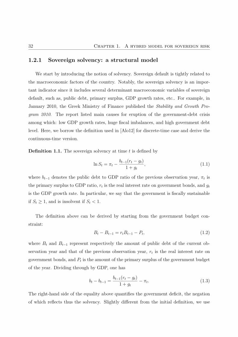
1.2.1 Sovereign solvency: a structural model
We start by introducing the notion of solvency. Sovereign default is tightly related tothe macroeconomic factors of the country. Notably, the sovereign solvency is an impor-tant indicator since it includes several determinant macroeconomic variables of sovereigndefault, such as, public debt, primary surplus, GDP growth rates, etc.. For example, inJanuary 2010, the Greek Ministry of Finance published the Stability and Growth Pro-gram 2010. The report listed main causes for eruption of the government-debt crisisamong which: low GDP growth rates, huge fiscal imbalances, and high government debtlevel. Here, we borrow the definition used in [Alo12] for discrete-time case and derive thecontinuous-time version.
Definition 1.1. The sovereign solvency at time t is defined by
lnSt = πt −bt−1(rt − gt)
1 + gt, (1.1)
where bt−1 denotes the public debt to GDP ratio of the previous observation year, πt isthe primary surplus to GDP ratio, rt is the real interest rate on government bonds, and gtis the GDP growth rate. In particular, we say that the government is fiscally sustainableif St ≥ 1, and is insolvent if St < 1.
The definition above can be derived by starting from the government budget con-straint:
Bt −Bt−1 = rtBt−1 − Pt, (1.2)
where Bt and Bt−1 represent respectively the amount of public debt of the current ob-servation year and that of the previous observation year, rt is the real interest rate ongovernment bonds, and Pt is the amount of the primary surplus of the government budgetof the year. Dividing through by GDP, one has
bt − bt−1 = bt−1(rt − gt)1 + gt
− πt. (1.3)
The right-hand side of the equality above quantifies the government deficit, the negationof which reflects thus the solvency. Slightly different from the initial definition, we use
1.2. Hybrid model of sovereign default time 33
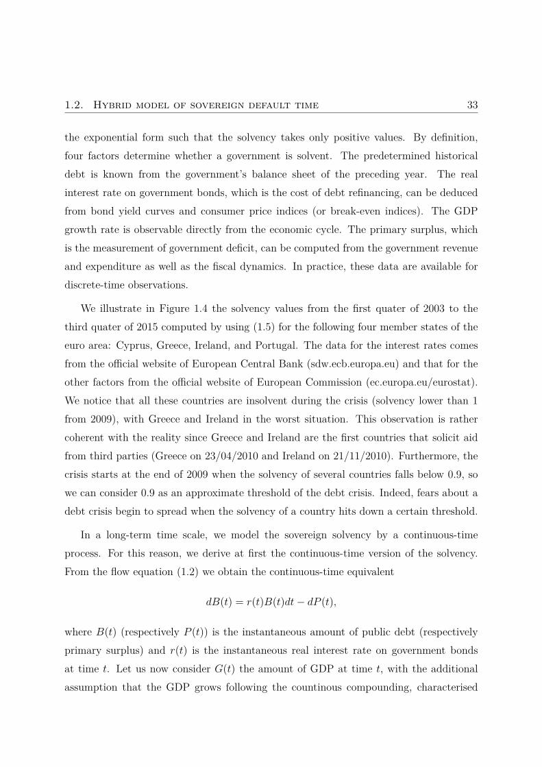
the exponential form such that the solvency takes only positive values. By definition,four factors determine whether a government is solvent. The predetermined historicaldebt is known from the government’s balance sheet of the preceding year. The realinterest rate on government bonds, which is the cost of debt refinancing, can be deducedfrom bond yield curves and consumer price indices (or break-even indices). The GDPgrowth rate is observable directly from the economic cycle. The primary surplus, whichis the measurement of government deficit, can be computed from the government revenueand expenditure as well as the fiscal dynamics. In practice, these data are available fordiscrete-time observations.
We illustrate in Figure 1.4 the solvency values from the first quater of 2003 to thethird quater of 2015 computed by using (1.5) for the following four member states of theeuro area: Cyprus, Greece, Ireland, and Portugal. The data for the interest rates comesfrom the official website of European Central Bank (sdw.ecb.europa.eu) and that for theother factors from the official website of European Commission (ec.europa.eu/eurostat).We notice that all these countries are insolvent during the crisis (solvency lower than 1from 2009), with Greece and Ireland in the worst situation. This observation is rathercoherent with the reality since Greece and Ireland are the first countries that solicit aidfrom third parties (Greece on 23/04/2010 and Ireland on 21/11/2010). Furthermore, thecrisis starts at the end of 2009 when the solvency of several countries falls below 0.9, sowe can consider 0.9 as an approximate threshold of the debt crisis. Indeed, fears about adebt crisis begin to spread when the solvency of a country hits down a certain threshold.
In a long-term time scale, we model the sovereign solvency by a continuous-timeprocess. For this reason, we derive at first the continuous-time version of the solvency.From the flow equation (1.2) we obtain the continuous-time equivalent
dB(t) = r(t)B(t)dt− dP (t),
where B(t) (respectively P (t)) is the instantaneous amount of public debt (respectivelyprimary surplus) and r(t) is the instantaneous real interest rate on government bondsat time t. Let us now consider G(t) the amount of GDP at time t, with the additionalassumption that the GDP grows following the countinous compounding, characterised

34 Chapter 1. A hybrid model for sovereign risk
Figure 1.4 – Solvency of four countries of euro area.
by the differential equation dG(t) = G(t)g(t)dt, where g(t) is the instantaneous GDPgrowth rate at time t. We assume that all the processes are continuous. Denoting by b(t)(respectively π(t)) the instantaneous debt-to-GDP (respectively surplus-to-GDP) ratio attime t, i.e., b(t) = B(t)/G(t) (respectively π(t) = P (t)/G(t)), one has
d
(B(t)G(t)
)= dB(t)
G(t) −B(t) dG(t)G2(t)
= r(t)B(t)− dP (t)G(t) − B(t)g(t) dt
G(t)
= (r(t)− g(t)) b(t) dt− d(P (t)G(t)
)− P (t)g(t) dt
G(t)
= [r(t)b(t)− g(t)b(t)− g(t)π(t)] dt− dπ(t).

1.2. Hybrid model of sovereign default time 35
Finally, the continuous-time version of (1.3) is written as
db(t) = [r(t)b(t)− g(t)b(t)− g(t)π(t)] dt− dπ(t). (1.4)
Similar to the discrete-time case, the negation of the right-hand side of the equality abovedefines the dynamic of the soveregn solvency, and we give the following definition beforethe modelling in a probability space.
Definition 1.2. The continuous-time sovereign solvency at time t is defined by
S(t) = S(0) + π(t)− π(0) +∫ t
0[g(s)π(s) + g(s)b(s)− r(s)b(s)] ds, (1.5)
where b(t) denotes the debt-to-GDP ratio, π(t) is the surplus-to-GDP ratio, r(t) is theinstantaneous real interest rate on government bonds, and g(t) is the instantaneous GDPgrowth rate.
Let (Ω,A,P) be a probability space equipped with a filtration F = (Ft)t≥0 satisfyingthe usual conditions, i.e., F0 contains all the P-null sets and F is right-continuous: Ft =Ft+ := ∩s>tFs. We recall the definitions of three types of stopping times in the AppendixA, Definition A.1–A.3 (see e.g. the book of Protter [Pro05, Chapter III.2] or the surveyof Nikeghbali [Nik06, Chapter 2.3] for details).
Let W = (Wt, t ≥ 0) be a standard Brownian motion which is F-adapted. For a givencountry, we assume that the solvency is governed by a process S = (St, t ≥ 0) satisfyingthe following diffusion:
dSt = µ(t, St)dt+ σ(t, St)dWt, S0 = x, (1.6)
where µ and σ are Lipschitz continuous functions such that∫ T
0|µ(t, St)|dt+
∫ T
0σ2(t, St)dt <∞
for any T > 0. Let L be a real positive constant with L < S0 which represents a thresholdof the debt crisis. More precisely, if S falls below L, we consider that the sovereignbecomes seriously insolvent, i.e., the risk of default is extremely high. Then, we define arandom time τ0 as the first hitting time of the barrier L by the solvency process S, i.e.,
τ0 = inft ≥ 0 : St < L, (1.7)

36 Chapter 1. A hybrid model for sovereign risk
with the convention inf ∅ =∞. Note that τ0 is a predictable F-stopping time. In general,the début (“entering time”) of a predictable random set is a predictable stopping time(Jacod and Shiryaev [JS13, Proposition 2.13]).
1.2.2 Critical political event
Generally speaking, when a sovereign becomes fiscally vulnerable, a political meetingwill be organised at which political decisions need to be made concerning the relevantsovereign country. In reality, a multitude of political events are involved during thesemeetings. In this section, we propose a simplified model to explore the political impact,while real situations tend to be more complicated and less transparent. For the concernedsovereign, the meeting date is a critical date and often comes shortly after the solvencybarrier hitting time τ0. In our model, we assume that the critical date coincides with thetime τ0. We also assume that the result of political decisions depends on some exogenousfactor, such as an economic or financial shock: if the shock has occurred before thecritical date, then the sovereign can possibly end up in default at τ0; otherwise, it receivesa financial aid package without immediate default at τ0. Indeed, the term financial aidpackage is perceived as any assistance from third parties with the aim of improving thesolvency of the country in debt crisis, including a bailout loan, a quantitative easing policy,etc., in return for which the beneficiary should take austerity measures to ameliorate itsfinancial situation. From an economic point of view, when the solvency is below thethreshold, an exogenous shock can make things worse so that the aids from third partieswill be too costly (for example, austerity policies can do harms to the economy and sopeople vote against it) and the political decisions are in favour of a sovereign default.
We model the exogenous shock by the jump of a Poisson process N = (Nt, t ≥ 0) withintensity λN > 0 which is independent of the filtration F. Then, the result of politicaldecisions depends on the value of N at the critical date τ0. More precisely, we define
ζ =
τ0, on Nτ0 ≥ 1,
∞, on Nτ0 = 0.(1.8)
The random time ζ takes into account both the sovereign solvency and the political

1.2. Hybrid model of sovereign default time 37
decisions. Obviously, ζ is not an F-stopping time. However, ζ is an honest time (e.g.Barlow [Bar78]), which by definition is Ft-measurable on ζ ≤ t. Definitely, the eventζ ≤ t implies τ0 ≤ t, then for any t ≥ 0,
1ζ≤tζ = 1ζ≤tτ0 = 1ζ≤t(t ∧ τ0),
where (t ∧ τ0) is Ft-measurable. We can make ζ a stopping time with respect to a largerfiltration: the progressive enlargement of F by ζ, namely the filtration Fζ = (F ζt )t≥0,where
F ζt := ∩s>t(σ(ζ ≤ u : u ≤ s) ∨ Ft), t ≥ 0.
We note thatPω : τ0(ω) = ζ(ω) <∞ = P(ζ <∞),
then ζ is an accessible stopping time with respect to Fζ .
1.2.3 Idiosyncratic credit risk: a Cox process model
In the book of Lando [Lan09], the author decomposes the structure of the intensity ofan individual firm into two independent components, one coming from a common factorand one being idiosyncratic. In our model, besides the macroeconomic and politicalimpacts, we also consider the credit risk related to the idiosyncratic financial circumstanceof the sovereign, and we adopt the widely-used Cox process model.
Let λ = (λt, t ≥ 0) be a nonnegative F-adapted process, and η be an A-measurableexponentially distributed random variable of unit parameter representing the idiosyncraticfactor, independent of both F∞ and the Poisson process N . In the literature on thecorporate credit risks, the default intensity can depend on the pre-default equity priceprocess. In our case, λ can depend on the solvency S, which in turn depends on commonfactors, i.e., the macroeconomic factors. For example, let λt = λ(t, St), where λ : R+ ×R+ → R+ is a function whose form differs from country to country. In general, theintensity λ is decreasing with respect to the solvency S and remains bounded when S
tends to +∞, which implies that in a healthy situation of solvency, the idiosyncraticdefault risk is limited. We call the process λ the idiosyncratic default intensity.

38 Chapter 1. A hybrid model for sovereign risk
We introduce the default hazard process Λ = (Λt, t ≥ 0) as Λt =∫ t
0 λs ds. Let ξ be thetime of default due to the idiosyncratic credit risk, given by a Cox process model, i.e.,
ξ := inf t ≥ 0 : Λt > η . (1.9)
By definition, for any t ≥ 0, one has ξ ≥ t = Λt ≤ η. As usual, the random time ξis a totally inaccessible stopping time with respect to the progressive enlargement of thefiltration F by ξ, namely the filtration Fξ = (F ξt )t≥0, where
F ξt = ∩s>t(σ(ξ ≤ u : u ≤ s) ∨ Ft), t ≥ 0.
1.2.4 Sovereign default time: a hybrid model
We now model the sovereign default by combining the economic and political influencesdescribed by ζ and the idiosyncratic credit risk described by ξ. We recall the partitiontheorem of any stopping time T . For any A-measurable set A, we denote by TA therestriction of T on A, defined by
TA(ω) =
T (ω), ω ∈A,
∞, ω /∈A.
Theorem 1.3 ([DM75],Theorem 81). Let T be an F-stopping time. There exists a unique(up to a P-null set) partition of the set T < ∞ into two sets A and B which belongto FT− such that TA is accessible and TB is totally inaccessible. The stopping time TA iscalled the accessible part of T while TB is called the totally inaccessible part of T .
Conversely, given two stopping times, one accessible, the other totally inaccessible,by taking the minimum, one can consider to construct a new stopping time (by makingprecise the filtration of course). In this way, let the sovereign default time be
τ := ζ ∧ ξ, (1.10)
which means that the sovereign default can result either from macroeconomic and politicalevents, or from its own idiosyncratic financial situations. This sovereign default modelhas a hybrid nature of both structural and reduced-form approaches.

1.2. Hybrid model of sovereign default time 39
We make some comparisons with the jump to default extended CEV credit risk model:
1. We note that the default time τ in our model is not bounded by its predictablecomponent τ0. In fact, on the set τ0 < ξ ∩ Nτ0 = 0, τ = ξ > τ0. If (St, t ≥ 0)follows a CEV diffusion, then the default time τ defined in (1.10) is an extensionof the jump to default extended CEV model in [CL06]. We refer the readers to[DL01b, DS02] for the background about the CEV process and we shall discuss theCEV case in detail in Section 1.3.3.2.
2. If the Poisson process intensity of the exogenous shock λN → 0, i.e., the externalenvironment of the sovereign is relatively stable, then the default never occursat τ0, and our model converges to a Cox process model. On the contrary, whenλN →∞, we have τ = τ0∧ξ. In this case, we recover the jump to default extendedCEV model for corporate credit risk.
1.2.5 Extension to re-adjusted solvency thresholds
In practice, if the debt and deficit situation of the sovereign is excessive and has no im-provement, the authorities may be less confident and consequently relax the requirementson the solvency barrier. For example, after the European Union and the InternationalMonetary Fund formally agreed a first bailout package for Greece, the European CentralBank has been forced to relax the lending rules by suspending the minimum credit ratingrequired on collateral, which lowers indirectly the requirements on the greek solvency,since the solvency is reflected by credit rating on the market. In this case, other criticalpolitical events may be gradually anticipated. This observation motivates us to extendthe hybrid model to the case of multiple critical dates where solvency thresholds can bere-adjusted.
Let n ∈ N, and L1, L2, . . . , Ln ∈ R+ such that S0 > L1 > L2 > . . . > Ln, representingdifferent levels of solvency requirements. We define a sequence of solvency barrier hitting

40 Chapter 1. A hybrid model for sovereign risk
times τini=1 as
τi = inft ≥ 0 : St < Li, i ∈ 1, . . . , n. (1.11)
The sequence τini=1 is increasing since the solvency requirements are decreasing. Whenthe solvency falls below a certain requirement Li, for i ∈ 1, . . . , n− 1, we assume that acritical political event is organised immediately at τi. If an exogenous shock has alreadyarrived before, then the sovereign can possibly default at τi and no more critical politicalevents will be planned; if no exogenous shock arrives before τi, the sovereign may obtaina financial aid to avoid an immediate default, which makes it possible to predetermineanother critical political event when the solvency falls below Li+1, and so on and so forth,until the requirements on the solvency are exhausted.
The exogenous factor is modelled by an inhomogeneous Poisson process N with inten-sity function λN(t), and we define a random time ζ∗ as
ζ∗ = τi, on Nτi−1 = 0 ∩ Nτi ≥ 1, i ∈ 1, . . . , n+ 1 (1.12)
with convention τ0 = 0 and τn+1 =∞. Note that for u ≥ 0, one has
1ζ∗>u =n+1∑i=1
1τi>u(1Nτi−1=0 − 1Nτi=0) =n+1∑i=1
1τi−1≤u<τi1Nτi−1=0. (1.13)
We can check that
P(∪ni=1ω : τi(ω) = ζ∗(ω) <∞) = P(ζ∗ <∞),
then ζ∗ is an accessible stopping time with respect to the progressive enlargement of F byζ∗, namely the filtration Fζ∗ = (F ζ
∗
t )t≥0, where
F ζ∗
t := ∩s>t(σ(ζ∗ ≤ u : u ≤ s) ∨ Fs), t ≥ 0.
Similar to the case of single critical date, the sovereign can be caused either by thesuccessive downgrade of solvency or by the idiosyncratic credit risk. Then, the sovereigndefault time is defined as
τ = ζ∗ ∧ ξ, (1.14)

1.2. Hybrid model of sovereign default time 41
where ξ is still given by (1.9). Let the global information structure be given as usual bythe progressive enlargement of the filtration F by the sovereign default time τ , denotedby G = (Gt)t≥0 and defined as
Gt =⋂s>t
(σ(τ ≤ u : u ≤ s) ∨ Fs
), t ≥ 0.
Then, τ is a G-stopping time. However, ζ∗ and ξ are not necessarily G-stopping time. Inorder to investigate the decomposition τ = ζ∗ ∧ ξ where all the three random times arestopping times, we need a still larger filtration. We denote by H = (H)t≥0 the progressiveenlargement of F by both ζ∗ and ξ. To be more precise, we set
Ht = ∩s>t(σ(ζ∗ ≤ u : u ≤ s) ∨ σ(ξ ≤ u : u ≤ s) ∨ Ft), t ≥ 0.
Obviously, Fζ∗ and Fξ are included in H.
Lemma 1.4. The following inclusion relations hold: F ( G ( H.
Proof: The first inclusion is obvious since τ is not an F-stopping time. For the secondinclusion, the σ-algebra
σ(τ ≤ s : s ≤ t) = σ(ζ∗ ≤ s ∪ ξ ≤ s : s ≤ t),
which is generated by the sets of the form ζ∗ ≤ s ∪ ξ ≤ s for any s ≤ t. On the onehand, one has G ⊆ H since
ζ∗ ≤ s ∪ ξ ≤ s ∈ σ(ζ∗ ≤ s : s ≤ t) ∨ σ(ξ ≤ s : s ≤ t);
on the other hand, the sets of the form ζ∗ ≤ s ∩ ξ ≤ s for any s ≤ t do not belong toσ(τ ≤ s : s ≤ t), which implies G 6= H. The lemma is thus proved.
The following proposition makes precise the unique partition of the set τ < ∞ onthe filtered probability space (Ω,A,H,P).
Proposition 1.5. Let τ be defined by (1.14) and let
A = ∪ni=1
(τi < ξ ∩ Nτi−1 = 0 ∩ Nτi ≥ 1
),
B = τ <∞/A.

42 Chapter 1. A hybrid model for sovereign risk
Then, A,B ∈ Hτ− and TA is accessible and TB is totally inaccessible, and τ = TA ∧ TB isthe unique decomposition a.s..
Proof: Firstly, the set τ < ∞ belongs to Hτ− since τ is measurable with respect toHτ−. Secondly, since τi is a predictable stopping time for any i = 1, . . . , n, by [Nik06,Theorem 2.23] one has
τi < ξ ∩ Nτi−1 = 0 ∩ Nτi ≥ 1 = τ = τi ∈ Hτ−,
which implies that A,B ∈ Hτ−. Furthermore, one can check that τA = ζ∗ and τB = ξ.Then, by Theorem 1.3, τ = τA ∧ τB is the unique decomposition up to a P-null set.
In this case, the stopping time τ is decomposed into an accessible part, which has npredictable components, and a totally inaccessible part.
1.2.6 Immersion property under minimum
In literature on the theory of enlargements of filtrations, we say that the couple (F,G)satisfies the immersion property or the so-called (H)-hypothesis (or F is immersed in G) ifany F-martingale remains a G-martingale. In the previous section, the sovereign defaulttime τ is defined as the minimum of two random times ζ∗ and ξ. In [Li12, Chapter6], the author has studied the problem of stability for the immersion property underminimum of two random times. More precisely, given two random times σi for i = 1, 2,if the immersion property holds between the reference filtration F and the respectiveprogressive enlargements of F by σi for i = 1, 2, the author gives conditions under whichthe immersion property is satisfied between F and the progressive enlargement of F byσ1 ∧ σ2. By using this result, we investigate separately the two parts of τ and prove,without computing explicitly the conditional probability distribution, that F is immersedin H and then by filtration shrinkage that (F,G) satisfies the immersion property.
It is well known (e.g., Bielecki and Rutkowski [BR02]) that if the random time ξis constructed by Cox process model, then the couple (F,Fξ) satisfies the immersionproperty. We prove that it is also the case for (F,Fζ∗).

1.2. Hybrid model of sovereign default time 43
Lemma 1.6. The immersion property holds for the couple (F,Fζ∗).
Proof: For any s, t ∈ R+ and s ≤ t, by (1.13) one has
P(ζ∗ ≤ s|F∞) = 1−n+1∑i=1
1τi−1≤s<τiP(Nτi−1 = 0|F∞).
The independence of the Poisson process and the filtration F implies that
P(Nτi−1 = 0|F∞) = P(Nτi−1 = 0|Ft)
on the set τi−1 ≤ s, which in turn implies
P(ζ∗ ≤ s|F∞) = P(ζ∗ ≤ s|Ft).
This last equality is (H5)-condition in Elliott, Jeanblanc and Yor [EJY00], which is equiv-alent to (H)-hypothesis.
Proposition 1.7. The filtration F is immersed in H.
Proof: For any c, k ∈ R+, by (1.13) one has
P(ζ∗ > c, ξ > k|F∞) =n+1∑i=1
1τi−1≤c<τiP(Nτi−1 = 0, ξ > k|F∞)
=n+1∑i=1
1τi−1≤c<τiP(Nτi−1 = 0, η > Λk|F∞).
Since both η and the Poisson process N are independent of F∞, we deduce that
P(Nτi−1 = 0, η > Λk|F∞) = P(Nτi−1 = 0, η > Λk|Ft)
on the set τi−1 ≤ c, which yields
P(ζ∗ > c, ξ > k|F∞) = P(ζ∗ > c, ξ > k|Ft).
By [Li12, Chapter 6, Lemma 6.2.4], the immersion property holds for the couple (F,H).
Since any F-martingale is G-adapted, Proposition 1.7 and [FP11, Theorem 2] implythat F is immersed in G (see also [Li12, Chapter 6, Lemma 6.2.3]).

44 Chapter 1. A hybrid model for sovereign risk
1.3 Probability of default on multiple critical dates
In this section, we are interested in the probability that the sovereign default occurson specific critical political dates. As we show, such default probabilities are nonzero inthe hybrid model, which implies singularities in the probability distribution of default.
1.3.1 Conditional default and survival probabilities
We consider the sovereign default given by the hybrid model (1.14). For any i ∈1, . . . , n, let the F-conditional probability that the sovereign default time τ coincideswith τi be denoted by pit := P(τ = τi|Ft), t ≥ 0.
Proposition 1.8. The process (pit, t ≥ 0) is an F-martingale stopped at τi and is given by
pit = E[(e−∫ τi−1
0 λN (s)ds − e−∫ τi
0 λN (s)ds)e−Λτi |Ft
], i = 1, . . . n, (1.15)
where we recall that λN is the time-dependent Poisson intensity.
Proof: The event τ = τi equals τi ≤ ξ,Nτi−1 = 0, Nτi ≥ 1. Since τi is an F-stoppingtime, the Poisson process N and the random variable η are mutually independent and inaddition independent of F, one has
P(τ = τi|F∞) = P(τi ≤ ξ,Nτi−1 = 0, Nτi ≥ 1|F∞)
= P(Λτi ≤ η,Nτi−1 = 0, Nτi ≥ 1|F∞)
= P(Λτi ≤ η|F∞)P(Nτi−1 = 0, Nτi ≥ 1|F∞)
= e−Λτi(e−∫ τi−1
0 λN (s)ds − e−∫ τi
0 λN (s)ds), (1.16)
which implies (1.15) and that pit is stopped at τi, i.e., pit∧τi = pit.
We notice from the above proposition that on the set τi ≤ t, pit does not dependon t, which means that the information concerning the impact of a political decision isneutralised after the event. In particular, we have
P(τ = τi) = pi0 = E[(e−∫ τi−1
0 λN (s)ds − e−∫ τi
0 λN (s)ds)e−Λτi
]. (1.17)

1.3. Probability of default on multiple critical dates 45
We now compute the F-conditional survival probability of the sovereign and re-visitthe immersion property.
Proposition 1.9. For all u, t ∈ R+, the F-conditional survival probability is given by
P(τ > u|Ft) = E[
exp(−
n∑i=1
1τi≤u∫ τi
τi−1λN(s)ds− Λu
)∣∣∣Ft]. (1.18)
Proof: For all u, t ∈ R+, by (1.13) one has
P(τ > u|Ft) = P(ζ∗ > u, ξ > u|Ft)
= E[( n+1∑
i=11τi−1≤u<τi1Nτi−1=0
)1ξ>u
∣∣∣∣Ft].If u ≤ t, then
P(τ > u|Ft) =n+1∑i=1
1τi−1≤u<τiE[1Nτi−1=01ξ>u
∣∣∣Ft]
=n+1∑i=1
1τi−1≤u<τiE[1Nτi−1=01η>Λu
∣∣∣Ft]
=( n+1∑i=1
1τi−1≤u<τie−∫ τi−1
0 λN (s)ds)e−Λu .
= exp(−
n+1∑i=1
1τi−1≤u<τi
∫ τi−1
0λN(s)ds
)e−Λu
= exp(−
n∑i=1
1τi≤u∫ τi
τi−1λN(s)ds− Λu
).
If u > t, we compute P(τ > u|Ft) as the Ft-conditional expectation of P(τ > u|Fu), whichimplies (1.18).
We can easily check that the couple (F,G) satisfies the immersion property. Definitely,by Proposition 1.9, when u ≤ t, the F-conditional probability does not depend on t, i.e.,
P(τ > u|Ft) = P(τ > u|Fu), u ≤ t.
This last equality is equivalent to (H)-hypothesis (see Elliott, Jeanblanc and Yor [EJY00]).
Corollary 1.10. For all t, T ∈ R+ such that t ≤ T , the G-conditional survival probabilityis given by
P(τ > T |Gt) = 1τ>tE[
exp(−
n∑i=1
1t<τi≤T∫ τi
τi−1λN(s)ds−
∫ T
tλs ds
)∣∣∣Ft]. (1.19)

46 Chapter 1. A hybrid model for sovereign risk
Proof: This is the direct result of the key lemma in Elliott, Jeanblanc and Yor (c.f.[EJY00, Lemma 3.1]). Precisely,
P(τ > T |Gt) = 1τ>tP(τ > T |Ft)P(τ > t|Ft)
= 1τ>t
E[e−∑n
i=1 1τi≤T∫ τiτi−1
λN (s)ds−∫ T
0 λs ds∣∣∣∣Ft]
e−∑n
i=1 1τi≤t∫ τiτi−1
λN (s)ds−∫ t
0 λs ds,
which finishes the proof.
1.3.2 Compensator process
The compensator and the intensity processes of default play an important role inthe reduced-form approach of credit risk modelling. In a hybrid model, however, thecompensator process of τ is in general discontinuous and the intensity does not necessarilyexist.
Recall that an increasing càdlàg F-predictable process ΛF is called F-compensatorprocess of a random time τ if the process (1τ≤t − ΛF
t∧τ , t ≥ 0) is a G-martingale. Theprocess ΛG = (ΛF
t∧τ , t ≥ 0) is called the G-compensator of τ . The general method forcomputing the compensator is given in [EJY00] (see also [JY78, Proposition 2]) by usingthe Doob-Meyer decomposition of the Azéma supermartingale. This theorem is recalledin Appendix A.
In the case where the immersion property holds, the Azéma supermartingale becomesa decreasing process and then A = 1 − G. In this case, G is the unique solution of thefollowing stochastic differential equation
dGt = −Gt−dΛFt , t > 0, G0 = 0.
The solution to the equation above is well-known: G = E(−ΛF), where E denotes theDoléan-Dade exponential ([Pro05, Chapter II, page 85]). More precisely,
Gt = E(−ΛF)t = exp(−ΛF
t −12[ΛF,ΛF]t
).
In the sovereign default model (1.14), the Azéma supermartingale has an explicit form

1.3. Probability of default on multiple critical dates 47
given by Proposition 1.9 as
Gt = P(τ > t|Ft) = exp(−∫ t
0λs ds−
n∑i=1
1τi≤t∫ τi
τi−1λN(s)ds
), t ∈ R+, (1.20)
which is a decreasing process. We can also compute the hazard process Γ ([BR02, Chapter5]) of the sovereign default time τ as
Γt = − lnGt =∫ t
0λs ds+
n∑i=1
1τi≤t∫ τi
τi−1λN(s)ds, t ∈ R+. (1.21)
By applying Ito’s formula for semimartingales to exp(−Γ), one has
e−Γt = −∫ t
0e−Γs−dΓs +
∑0<s≤t
(e−Γs − e−Γs− + e−Γs−)∆Γs,
where ∆Γt = Γt − Γt−. By consequence, we obtain
ΛFt = −
∫ t
0
dGs
Gs−= −
∫ t
0
de−Γs
e−Γs−= Γt +
∑0<s≤t
(1− e−∆Γs −∆Γs
),
which yields the following relationship between the processes ΛF and Γ
ΛFt = Γct +
∑0<s≤t
(1− e−∆Γs
), t ∈ R+,
where Γc is the continuous part of Γ. Thus, the F-compensator is
ΛFt =
∫ t
0λs ds+
n∑i=1
1τi≤t(
1− e−∫ τiτi−1
λN (s)ds), t ∈ R+, (1.22)
and the G-compensator is
ΛGt =
∫ t∧τ
0λs ds+
n∑i=1
1τi≤t∧τ(
1− e−∫ τiτi−1
λN (s)ds), t ∈ R+. (1.23)
We underline that the intensity process of sovereign default does not exist because of thediscontinuity of the compensator process at the F-stopping times (τi)ni=1. In literature,Gehmlich and Schmidt [GS16] provide a class of examples where the Azéma supermartin-gale contains jumps and propose a generalisation of this class with an additional stochasticintegral containing singularities at predictable stopping times.
We observe that the absolutely continuous part of ΛF and that of Γ are identical anddepend on the idiosyncratic default intensity λ, while their jump parts are different anddepend on the solvency (through the political critical dates) and the exogenous shock.When the external shock is small (λN(t) is small), we can approximate ΛF by Γ.

48 Chapter 1. A hybrid model for sovereign risk
Remark 1.11. It is known that if the compensator process is continuous, then so is thehazard process and the two processes coincide with each other ([BR02, Proposition 6.2.2]).Bélanger, Shreve and Wong ([BSW04]) has pointed out that when there are jumps in theAzéma supermartingale, the hazard process defined in their paper (which is technicallythe F-compensator) differs from the one defined in [BR02]. In the sovereign default modelpreviously mentionned in this section, we provide an example where the hazard processis not equal to the F-compensator.
1.3.3 Default probability in a Markovian setting
The general form of the sovereign default probability at critical dates pit, i = 1, . . . , n,is given by Proposition 1.8. We now consider several specific settings and provide ex-plicit formulae when the solvency process is a geometric Brownian motion or a ConstantElasiticity of Variance (CEV) process.
We first make some simplified assumptions. We assume that the equation (1.6) ishomogeneous and that the solvency process is given by
dSt = µ(St)dt+ σ(St)dWt, S0 = x,
where µ(·) : R+ → R and σ(·) : R+ → R+ satisfy regular enough conditions for theexistence and the pathwise uniqueness of a strong solution Sxt , t ≥ 0. Recall that theexistence and pathwise uniqueness holds in each of the following cases (see e.g. Oksendal[Oks03, Theorem 5.2.1] and Revuz and Yor [RY99, Theorem 3.5] for details):
(a) µ and σ are Lipschitz continuous, and for any x ∈ R+ there exists a constant Csuch that |µ(x)|+ |σ(x)| ≤ C(1 + |x|);
(b) µ is Lipschitz continuous, and for any x, y ∈ R+, |σ(x)− σ(y)|2 ≤ ϕ(|x− y|);(c) µ and σ are bounded, and for any x, y ∈ R+, |σ(x)−σ(y)|2 ≤ ϕ(|x−y|), σ ≥ ε > 0;(d) µ is bounded, and for any x, y ∈ R+, |σ(x) − σ(y)|2 ≤ |g(x) − g(y)| where the
function g : R+ → R is increasing and bounded, σ ≥ ε > 0.Let L denote the generator of S, i.e., for any function f ∈ C2 : R+ → R,
Lf(z) = µ(z)f ′(z) + 12σ
2(z)f ′′(z).

1.3. Probability of default on multiple critical dates 49
The technical hypotheses in [CL06] remain valid here with suitable financial interpre-tation. We specify the idiosyncratic intensity as a decreasing function of the solvency,i.e., λt = λ(St) with λ(·) : R+ → R+ being decreasing. When the solvency S → ∞, thesovereign has almost no chance to default, then λ should remain bounded. When S → 0,the solvency is bad enough to trigger a default, so that the idiosyncratic default intensitycan explode to infinity in this case.
Suppose in addition that the intensity of the exogenous shock is constant, so in theinhomogeneous Poisson process, the intensity function is λN(t) = λN > 0 for any t ≥0. Furthermore, we specify the idiosyncratic default intensity process λ as a decreasingfunction of the solvency λt = λ(St) with λ(·) : R+ → R+ being decreasing.
We consider the Laplace transform for the F-stopping time
ρx := inft ≥ 0 : Sxt ≤ L with Sx0 = x.
For any k ≥ 0, let
Q(x; k, L) := E[
exp(− kρx −
∫ ρx
0λ(Sxu) du
)]. (1.24)
Intuitively, if the process S starts from a higher level than x, then it takes on averagemore time to hit the threshold L, and so the function in (1.24) should be decreasing.However, this is not necessarily true when the process S is inhomogeneous.
Proposition 1.12. The parameterised function Q(·; k, L) defined in (1.24) is decreasing.
Proof: For any ω ∈ Ω, any x, x′ ∈ R+ such that x ≤ x′, define the F-stopping times
ρx′,x(ω) := inft ≥ 0 : Sx′t (ω) ≤ x and
ρx′(ω) := inft ≥ 0 : Sx′t (ω) ≤ L with Sx′
0 (ω) = x′.
The random time ρx is in distribution equal to ρx′ − ρx′,x, then by pathwise uniqueness

50 Chapter 1. A hybrid model for sovereign risk
and markovian properties one has
Q(x′; k, L) = E[exp
(− k(ρx′ − ρx′,x + ρx′,x)−
∫ ρx′
ρx′,x
λ(Sx′u )du−∫ ρx′,x
0λ(Sx′u )du
)]
≤ E[exp
(− k(ρx′ − ρx′,x)−
∫ ρx′
ρx′,x
λ(Sx′u )du)]
= E[exp
(− kρx −
∫ ρx
0λ(Sxu)du
)]= Q(x; k, L)
since kρx′,x +∫ ρx′,x0 λ(Sx′u )du ≥ 0. The proposition is thus proved.
It is difficult to compute directly the right-hand side of (1.24). However, one can provethat (1.24) is the representation of the solution to a differential equation. Then one cancompute the Laplace transform by solving an ODE.
Theorem 1.13. The right-hand side of (1.24) is the representation of the solution to thefollowing Dirichlet problem
Lu(z)− (λ(z) + k)u(z) = 0 on z > L;
u(L) = 1. (1.25)
Proof: Indeed, since ρx is a predictable stopping time, there exists an increasing se-quence of stopping times (ρm)m≥1 such that ρm < ρx and limm→∞ ρm = ρx P-a.s.. Let
βxt = exp(−∫ t
0(k + λ(Sxs ))ds
)for any t ≥ 0. By Ito’s formula, on the set t < ρx one has
d(βxt u(Sxt )) = −u(Sxt )βxt (k + λ(Sxt ))dt+ βxt Lu(Sxt )dt+ βxt u′(Sxt )σ(Sxt )dWt
= βxt u′(Sxt )σ(Sxt )dWt, (1.26)
where u is a solution to the Dirichlet problem (1.25). We then have
E[βxρmu(Sxρm)]− u(x) = E[∫ ρm
0βxs u
′(Sxs )σ(Sxs )dWs
],
where the right-hand side vanishes thanks to the boundedness of β, the smoothness of u.Thus, when m tends to +∞,
u(x) = E[βxρxu(L)] = E[exp
(−∫ ρx
0(λ(Sxs ) + k)ds
)].

1.3. Probability of default on multiple critical dates 51
The theorem is thus proved.
We refer the reader to Karatzas and Shreve [KS02, Chapter 5, Proposition 7.2] andTouzi [Tou13, Theorem 2.8] for a general representation of this kind of Dirichlet problem.
The probability that the sovereign bankruptcy occurs on a critical political date canbe derived from Q(·; k, L).
Proposition 1.14. The F-martingale (pit, t ≥ 0), i ∈ 1, . . . , n, is computed as
pit = e−∫ t∧τi
0 λ(Su)duQ(St∧τi−1 ;λN , Li−1)
·[e−λ
N (t∧τi−1)Q(S(t∧τi)∨τi−1 ; 0, Li)− e−λN (t∧τi)Q(S(t∧τi)∨τi−1 ;λN , Li)
], t ≥ 0,
(1.27)with L0 = S0 = x.
Proof: By Proposition 1.8 and the section assumptions, we have for any i ∈ 1, . . . , nand t ∈ R+ that
pit = E[(e−λN τi−1 − e−λN τi)e−
∫ τi0 λ(Su)du
∣∣∣Ft] .Since pi is a martingale stopped at τi, it suffices to compute pit on the set t < τi. Onthe set τi−1 ≤ t < τi, by the Markovian property of the process S, we obtain
pit = e−λN τi−1E
[e−∫ τi
0 λ(Su)du∣∣∣Ft]− E
[e−λ
N τi−∫ τi
0 λ(Su)du∣∣∣Ft]
= e−∫ t
0 λ(Su)du[e−λ
N τi−1Q(St; 0, Li)− e−λN tQ(St;λN , Li)
].
In particular, one has
piτi−1= e−λ
N τi−1−∫ τi−1
0 λ(Su)du[Q(Li−1; 0, Li)−Q(Li−1;λN , Li)
],
which yields that on the set t < τi−1,
pit = e−λN t−
∫ t0 λ(Su)duQ(St;λN , Li−1)
[Q(Li−1; 0, Li)−Q(Li−1;λN , Li)
].
Finally, we note that Q(Sτi−1 ; k, Li−1) = Q(Li−1; k, Li−1) = 1 for any k, which implies(1.27).
The proposition above shows that it is essential to compute the quantity Q(x; k, L) toobtain explicit form of the probabilities of default at critical political events. We presentbelow explicit formulae for two widely used cases.

52 Chapter 1. A hybrid model for sovereign risk
1.3.3.1 Case of geometric Brownian motion
Let the solvency process S be a geometric Brownian motion which is the solution to
dSt = St(µdt+ σdWt), t ≥ 0,
where W is a standard Brownian motion, µ, σ ∈ R with σ > 0 and S0 = x. Similar as in[CL06], we suppose that the idiosyncratic default intensity λ is a decreasing function ofthe solvency S:
λt = λ(St) = a
S2βt
+ b, (1.28)
where a > 0, b, β ≥ 0 represent respectively the scale parameter governing the sensitivityof λ to S, the constant lower bound and the elasticity parameter. Then, by (1.25),u(x) = Q(x; k, L) is the solution to the following Sturm-Liouville equation (see [Eve05]):
12σ
2x2u′′(x) + µxu′(x)− (ax−2β + b+ k)u(x) = 0 on (L,+∞);
u(L) = 1.(1.29)
Case β = 0: Let k = a+ b+ k. Then, the equation (1.29) becomes
12σ
2x2u′′(x) + µxu′(x)− ku(x) = 0, (L,+∞);
u(L) = 1,(1.30)
to which the fundamental solution has the form xγ, where γ ∈ R is a constant to beidentified. Then, one can compute that γ1,2 = −ν ±
√ν2 + 2k
σ2 , where ν = µ/σ2 − 1/2.The general solution to the equation (1.30) has the form
u(x) = A1xγ1 + A2x
γ2 ,
where A1, A2 ∈ R. Since u(x) is bounded when x→∞, we deduce that A1 = 0, and theboundary condition u(L) = 1 yields A2 = L−γ2 .
Apart from solving the equation (1.30), one can also compute directly the expectationE[e−kρx ]. Precisely,
St = xe(µ−σ22 )t+σWt = xeσWt , t ≥ 0,

1.3. Probability of default on multiple critical dates 53
where Wt = νσt+Wt, and the first hitting time ρx can be defined equivalently as
ρx = inft ≥ 0 : Wt ≤1σ
ln(L/x).
By Girsanov’s theorem, we can define a probability P under which W is a Brownianmotion. The Radon-Nikodym density of P with respect to P restricted on Ft is given by
dPdP
∣∣∣∣Ft
= eνσWt− 12ν
2σ2t, t ≥ 0.
Then, by a change of probability one has
E[e−kρx
]= E
[expνσWρx −
12ν
2σ2ρx − kρx]
=(L
x
)νE[exp
−(1
2ν2σ2 + k
)ρx
],
where E denotes the expectation under the probability P. Since the process(exp
−√ν2σ2 + 2kWt∧ρx − (ν2σ2/2 + k)(t ∧ ρx)
, t ≥ 0
)
is bounded by e−√ν2σ2+2k(lnL−lnx)/σ, it is a uniformly integrable P-martingale. Doob’s
optional sampling theorem (e.g. [Pro05, Theorem 16]) yields the same result (see c.f.[BS02, Part II, Chapter 9, 2.0.1])
Q(x; k, L) =(L
x
)√ν2+2k/σ2+ν.
Case β > 0: We let w(z) = u(z−1β )z−
νβ . Then, w satisfies the following Bessel equation
in a modified form (e.g. [Eve05, Chapter 17])
(zw′(z))′ − 1β2
(ν2 + 2(k + b)/σ2
)z−1w′(z) = 2az
β2σ2w(z), z ∈ (0, L−β). (1.31)
Let ψ = 1β
√ν2 + 2(k + b)/σ2, then the equation above admits two linearly independent
fundamental solutions Iψ(z√
2a/σβ) and Kψ(z√
2a/σβ), where I and K are modifiedBessel functions of the first and second kind, and are defined by
Iψ(x) :=∞∑i=0
(x/2)ψ+2i
i!Γ(ψ + i+ 1) ,
Kψ(x) := π
2I−ψ(x)− Iψ(x)
sin(ψπ) ,

54 Chapter 1. A hybrid model for sovereign risk
with Γ being the gamma function. Then, the general solution to the equation (1.31) hasthe form
w(z) = B1Iψ(z√
2a/σβ) +B2Kψ(z√
2a/σβ),
where B1, B2 ∈ R. The modified Bessel functions have the following asympthotic be-haviours when z → 0 (see e.g. [BS02, Appendix 2.4]):
Iψ(z) ' 1Γ(ψ)
(z
2
)ψ,
Kψ(z) ' Γ(ψ)2
(z
2
)−ψ, ψ > 0, K0(z) ' − ln z.
The boundedness of u(z−1β ) as z → 0 implies that B2 = 0 and the boundary condition
u(L) = 1 yields B1 = Lν/Iψ(√
2a/σβLβ). Thus, we have (see also [Ken78, Theorem 3.1]and [BS02, Part II, Chapter 9, 2.8.3])
Q(x; k, L) = w(x−β)xν
=(L
x
)ν Iψ(√
2a/σβxβ)Iψ(√
2a/σβLβ).
We can notice that, in the both cases, when the threshold L tends to 0, Q(x; k, L) → 0,which implies that the sovereign bankrupt occurs on a critical political date with zeroprobability. This is because the solvency process modelled by a geometric Brownianmotion never hits 0.
1.3.3.2 Case of the CEV process
In practice, for sovereigns in severe financial crise (e.g. Greece), the volatility of thesolvency fluctuates notably over time. We now consider another widely used process inthe financial industry, the CEV model in which the volatility is a monotonic function ofthe solvency. Let the solvency process be a CEV process driven by the following diffusion
dSt = µSt dt+ δSβ+1t dWt, S0 = x, (1.32)
where β ∈ R and δ > 0 are respectively the elasticity parameter and the scale parameterof the volatility. In particular, the process S is a geometric Brownian motion if β = 0.We distinguish two cases according to the sign of β. For β < 0, the volatility σ(S) = δSβ

1.3. Probability of default on multiple critical dates 55
is a decreasing function of S. From a financial point of view, when the solvency decreases,lower solvency (higher deficit) indicates higher level of government borrowing, leadingto lower growth rate, as well as smaller future expenditure to improve the budgetarysituation. All these add more uncertainty to the solvency. For β > 0, the volatility isan increasing function of S. Namely, when the solvency increases, besides higher growthrate, higher solvency (surplus) may imply higher fiscal revenue which the governmentis under pressure to disburse for social welfare, also making the solvency become moreuncertain. In other words, the volatility has the possibility to be either an increasing or adecreasing function of the solvency. We note in addition that when β > 0, the conditionsfor the existence and the pathwise uniqueness of a strong solution are not satisfied and theprocess S is a strictly local martingale (c.f. [EM82]) , which describes situations wherebubbles may exist on financial market. To remedy the situation, one needs to regularisethe process for large values (see Davydov and Linetsky [DL01b, Appendix C] for details).
Recall that the CEV diffusion has the following boundary characterisation. For β < 0,+∞ is a natural boundary and zero is reached almost surely. For −1/2 ≤ β < 0, zerois an absorbing boundary. For β < −1/2, zero is a reflecting boundary. For β = 0, theCEV process reduces to a geometric Brownian motion, and both zero and +∞ are naturalboundaries. For β > 0, zero is a natural boundary and +∞ is an entrance boundary.
The specification of the idiosyncratic default intensity λ(S) depends on the sign of theparameter β. More precisely, when β > 0 (respectively β < 0), λ(S) is an affine functionof 1
σ2(S) (respectively σ2(S)), i.e.,
λ(S) = a
S2|β| + b, a > 0, b ≥ 0, β ∈ R. (1.33)
Then, u(x) = Q(x; k, L) is the decreasing solution of the following equation:
12δ
2x2+2βu′′ + µxu′ − (ax−2|β| + b+ k)u = 0, on (L,+∞);
u(L) = 1.(1.34)
The fundamental solutions to this last equation are different according to the sign of β.
In the following, we consider separately the two cases according to the sign of β. Inliterature, the case β < 0 has been studied for the valuation of path-dependent options

56 Chapter 1. A hybrid model for sovereign risk
in [Lin04] and the jump to default CEV model in [MACL10, MAL11]. The case β > 0is more unusual. We shall use another similar equation, called CEV ordinary differentialequation (ODE), which has been studied in [DL01b] where the coefficient of u is a negativeconstant. We make use of the knowledge of the solutions to the CEV ODE to solve theequation (1.34).
Case β > 0: We let v(x) = u(x)eκx−2β , where κ = 12βδ2 (√µ2 + 2aδ2 − µ) > 0. Then, v
satisfies the following CEV ODE:
12δ
2x2+2βv′′ +√µ2 + 2aδ2xv′ −
(κβ(2β + 1)δ2 + b+ k
)v = 0, x ∈ (L,∞). (1.35)
The equation above corresponds to another CEV diffusion:
dxt = xt(√µ2 + 2aδ2 dt+ δxβt dWt), t ≥ 0,
for which +∞ is an entrance boundary. Then, the equation (1.35) admits two linearlyindependent fundamental solutions v+ and v−, respectively increasing and decreasing,satisfying the following boundary conditions at +∞ ([BS02, pages 18-19]):
limx→+∞
v+(x) = +∞, limx→+∞
v−(x) > 0,
and the generaly solution to the equation (1.35) has the form
v(x) = C1v+(x) + C2v−(x),
where C1, C2 ∈ R. Since u(x) is bounded as x → ∞, so is v(x), and we deduce thatC1 = 0, C2 = e−κ/L
2β/v−(L). The decreasing fundamental solution v− is given by [DL01b,
Proposition 5] as
v−(x) = xβ+ 12 e
√µ2+2aδ22βδ2
x−2βMn,m
(√µ2 + 2aδ2
βδ2 x−2β),
where n = 12+ 1
4β−κβ(2β+1)δ2+b+k
2β√µ2+2aσ2
= µ(2β+1)+2b+2k4β√µ2+2aδ2
,m = 14β andMn,m(z) := zm+1/2e−z/2F1(m−
n+ 1/2, 2m+ 1, z) is Whittaker function of the first kind with
F1(a, b, z) := 1 +∞∑j=1
a(a+ 1) . . . (a+ j − 1)zjb(b+ 1) . . . (b+ j − 1)j!

1.3. Probability of default on multiple critical dates 57
being Kummer confluent hypergeometric function of the first kind. This fundamentalsolution implies that
Q(x; k, L) = C2v−(x)e−κ/x2β =xβ+ 1
2 eµ
2βδ2x−2β
Mn,m
(√µ2+2aδ2
βδ2 x−2β)
Lβ+ 12 e
µ
2βδ2L−2β
Mn,m
(√µ2+2aδ2
βδ2 L−2β) ,
which is valid for any µ ∈ R.
Case β < 0: We let y(z) = u(z1γ )z
12−
12γ , where
γ =
√
1 + 8a/δ2, µ > 0,
−√
1 + 8a/δ2, µ ≤ 0.
If γ < −1, y is an increasing function on (0, Lγ) and limz→0+ y(z) = 0; if γ > 1, y isa decreasing function on (Lγ,+∞) and limz→+∞ y(z) = 0. Moreover, y satisfies anotherCEV ODE as follows:
12δ
2γ2z2+2βy′′ + µγzy′ −(b+ k + µγ − µ
2
)y = 0, (1.36)
where β = βγ, the sign of which depends on the sign of µ, and we note that b+k+ µγ−µ
2 > 0for any µ ∈ R. The equation above corresponds to another CEV diffusion:
dzt = γzt(µ dt+ δzβt dWt), t ≥ 0.
The equation (1.36) has two linearly independent solutions y+ (increasing) and y− (de-creasing), and the general solution is the linear combination of y+ and y−.
If β < 0 (namely µ > 0 and γ > 1), then +∞ is a natural boundary, and one has
limz→+∞
y−(z) = 0 and limz→+∞
y+(z) = +∞
and hence y is proportional to y−. If β > 0 (namely µ ≥ 0 and γ < −1), then 0 is anatural boundary, and one has
limz→0+
y−(z) = +∞ and limz→0+
y+(z) = 0
and hence y is proportional to y+. Therefore, by [DL01b, Proposition 5], when µ 6= 0there exists a constant D > 0 such that
y(z) = Dzβγ
+ 12 e
µ
2βδ2z−2β/γ
Wn′,m′
(− |µ|βδ2 z
−2β/γ),

58 Chapter 1. A hybrid model for sovereign risk
where n′ = sgn(µβ)(12 + γ
4β ) − 2b+2k+µγ−µ4|µβ| = 2b+2k−µ(2β+1)
4|µ|β , m′ = − |γ|4β = −√
1+8a/δ2
4β andthe function Wn,m(x) := xm+1/2e−x/2F2(m− n+ 1/2, 2m+ 1, x) is Whittaker function ofthe second kind with
F2(a, b, x) := Γ(1− b)Γ(1 + a− b)F1(a, b, x) + Γ(b− 1)
Γ(a) x1−bF1(1 + a− b, 2− b, x)
being Kummer confluent hypergeometric function of the second kind. One can computethe constant D by using the relation y(Lγ) = Lγ/2−1/2. If µ = 0 and thus γ < −1 andβ > 0, then
y(z) = Dy+(z) = D√zK2m′
(−z−β/γ
δβ
√2b+ 2k + µγ − µ
),
where Kψ(x) is modified Bessel function of the second kind, defined as
Kψ(x) := π
2 sin(ψπ) (I−ψ(x)− Iψ(x)) .
Therefore we obtain
Q(x; k, L) = y(xγ)x 12−
γ2 =
xβ+ 12 e
µ
2βδ2x−2β
Wn′,m′
(− |µ|βδ2
x−2β)
Lβ+ 12 e
µ
2βδ2L−2β
Wn′,m′
(− |µ|βδ2
L−2β) , µ 6= 0,
√xK2m′
(−x−βδβ
√2b+2k+µγ−µ
)√LK2m′
(−L−β
δβ
√2b+2k+µγ−µ
) , µ = 0.
1.3.4 Numerical illustrations
We now present numerical examples to illustrate the results obtained previously con-cerning the sovereign default probability and the defaultable bond yield. s
In the first example, we are interested in the default probability pi0 on a political criticaldate τi, (i = 1, 2, 3), given by (1.17). We assume that the solvency process S is modelled bya geometric Brownian motion as in Section 1.3.3.1, and we use the solvency data of Greeceduring the period from 2003 to 2013 to estimate the parameters and obtain S0 = 1.01,µ = −0.01 and σ = 0.14. Let the idiosyncratic default intensity process λ be specifiedby λ(S) = a
S2β + b as in (1.28) and the Poisson intensity be a constant λN . The solvencybarrier is re-adjustable with three values L1 = 0.9, L2 = 0.8 and L3 = 0.7. Figure 1.5
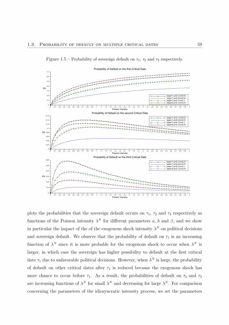
1.3. Probability of default on multiple critical dates 59
Figure 1.5 – Probability of sovereign default on τ1, τ2 and τ3 respectively.
plots the probabilities that the sovereign default occurs on τ1, τ2 and τ3 respectively asfunctions of the Poisson intensity λN for different parameters a, b and β, and we showin particular the impact of the of the exogenous shock intensity λN on political decisionsand sovereign default. We observe that the probability of default on τ1 is an increasingfunction of λN since it is more probable for the exogenous shock to occur when λN islarger, in which case the sovereign has higher possibility to default at the first criticaldate τ1 due to unfavorable political decisions. However, when λN is large, the probabilityof default on other critical dates after τ1 is reduced because the exogenous shock hasmore chance to occur before τ1. As a result, the probabilities of default on τ2 and τ3
are increasing functions of λN for small λN and decreasing for large λN . For comparisonconcerning the parameters of the idiosyncratic intensity process, we set the parameters

60 Chapter 1. A hybrid model for sovereign risk
a = 0.1, b = 0.01 and β = 1 and examine the impact of each parameter by consideringvalues a = 0.5, b = 0.1 and β = 4 respectively. Other things being equal, the probabilitiesof default on τ1, τ2 and τ3 are smaller for bigger a (respectively bigger b) because it ismore probable for the sovereign to default due to the idiosyncratic credit risk when λ(S)is bigger. The impact of the elasticity parameter β depends on the level of solvency, moreprecisely, λ(S) is decreasing (respectively increasing) when S ≥ 1 (respectively S < 1).Consequently, the probability of default on τ1 (respectively τ2, τ3) is smaller for smallerβ (respectively bigger β).
Figure 1.6 – Sovereign default probability.
In the second example, we consider the sovereign default probability P(τ ≤ T ), whichcan be computed by Proposition 1.9. The solvency process S is given as a geometricBrownian motion with the same parameters as in the previous example. We fix the valuesof a = 0.1, b = 0.01 and β = 1 for idiosyncratic default intensity. Figure 1.6 plotsthe probability of default from 1 to 30 years for different values λN = 0, 0.05 and 0.2

1.4. Hybrid model beyond immersion paradigm 61
respectively. We note that an exogenous shock with larger intensity value increases thesovereign default probability.
1.4 Hybrid model beyond immersion paradigm
The links between the market completeness and the immersion property have beenstudied in the credit risk literature (e.g. [JLC09a]). The advantage of the immersionis that the market risk premium takes into account the jump risk premium and so therisk-neutral probability does not need to be changed. However, it is usually impossibleto assume the immersion property in the cases of incomplete market, non-ordered multi-defaults, and correlation between different default times. For this reason, we tend toadapt our model to a more general level.
The discussions in Subsection 1.2.6 show that the immersion property of the couple(F,G) preserved by the model results principally from the independence between therandom barrier η and F∞ in the Cox process model when we define the totally inaccessiblepart of the default time. In order to obtain a model without immersion, similar to[EKJJZ14, Section 4.2], we relax the assumption that the random variable η is independentof F∞ by simply assuming that the F-conditional probability distribution of η is absolutelycontinuous. We make the following density hypothesis.
Assumption 1.15. We assume that η is a positive random variable whose conditionalprobability distribution with respect to F admits a density process, i.e., there exists anFt ⊗ B(R+)-measurable function βt(u) such that
P(η > θ|Ft) =∫ ∞θ
βt(u)du.
This assumption made on a random barrier is especially useful in studies on insidertrading (see e.g. [GP98]). By the fact that Λ is increasing and absolutely continuous
P(η > Λu|Ft) =∫ ∞
Λuβt(s)ds =
∫ ∞u
βt(Λs)λs ds.
One can re-compute the conditional default and survival probabilities in the new setting.

62 Chapter 1. A hybrid model for sovereign risk
On the set τi ≤ t, one has
P(τ = τi|Ft) = P(τi < ξ,Nτi−1 = 0, Nτi ≥ 1|Ft)
= P(Λτi < η,Nτi−1 = 0, Nτi ≥ 1|Ft)
= P(Λτi < η|Ft)P(Nτi−1 = 0, Nτi ≥ 1|Ft)
=(e−∫ τi−1
0 λN (s)ds − e−∫ τi
0 λN (s)ds) ∫ ∞
τiβt(Λs)λs ds,
and on τi > t, we compute P(τ = τi|Ft) as the Ft-conditional expectation of P(τ =τi|Fτi). Furthermore, if u ≤ t, then
P(τ > u|Ft) = E[( n+1∑
i=11τi−1≤u<τi1Nτi−1=0
)1ξ>u
∣∣∣∣Ft]
=n+1∑i=1
1τi−1≤u<τiE[1Nτi−1=01ξ>u
∣∣∣Ft]
=n+1∑i=1
1τi−1≤u<τiE[1Nτi−1=01η>Λu
∣∣∣Ft]
= exp(−
n+1∑i=1
1τi−1≤u<τi
∫ τi−1
0λN(s)ds
) ∫ ∞u
βt(Λs)λs ds
= exp(−
n∑i=1
1τi≤u∫ τi
τi−1λN(s)ds
) ∫ ∞u
βt(Λs)λs ds.
If u > t, we compute P(τ > u|Ft) as the Ft-conditional expectation of P(τ > u|Fu).
Let Zt =∫∞t βt(Λs)λs ds, which is an F-supermartingale. Then the Azéma super-
martingale of τ is
Gt = Zt exp(−
n∑i=1
1τi≤t∫ τi
τi−1λN(s)ds
).
It is much more difficult to compute the compensator process because the additive form ofthe Doob-Meyer decomposition of G is difficult to be performed when G has a multiplica-tive form. It is well known that a nonnegative càdlàg supermartingale can be uniquelyfactorised as a positive local martingale multiplied by a decreasing process (see e.g. Itoand Watanabe [IW65]). By [EKJJ10, Proposition 4.1], the Doob-Meyer decomposition ofZ is given by
Zt = 1 +Mt −∫ t
0βs(Λs)λs ds,

1.4. Hybrid model beyond immersion paradigm 63
where M is the càdlàg square integrable F-martingale defined by
Mt =∫ t
0λs[βs(Λs)− βt(Λs)]ds, a.s..
Let θ = inft ≥ 0 : Zt− = 0 and define γt = βt(Λt)λtZt−
on t < θ, then the factorisation ofZ is given by
Zt = Lt exp(−∫ t
0γs∧θds
),
where L is a positive F-local martingale solution to the SDE
dLt = e∫ t
0 γs∧θdsdMt, L0 = 1,
which implies the multiplicative decomposition of G:
Gt = Lt exp(−∫ t
0γs∧θds−
n∑i=1
1τi≤t∫ τi
τi−1λN(s)ds
). (1.37)
Again, we refer the readers to Gehmlich and Schmidt [GS16], where a class of examplesof Azéma supermartingale containing jumps are provided.
On the other hand, by [Jac79, Corollaire 6.35] and the uniqueness of the factorisationof G, one has
Gt = LtE(−ΛFt ) = Lte
−ΛF,ct
∏0<s≤t
(1−∆ΛFs ),
where ΛF,c is the continuous part of ΛF, and by comparison, we obtain the F-compensator
ΛFt =
∫ t
0γs∧θds+
n∑i=1
1τi≤t(
1− e−∫ τiτi−1
λN (s)ds), t ∈ R+, (1.38)
and the G-compensator
ΛGt =
∫ t∧τ
0γs∧θds+
n∑i=1
1τi≤t∧τ(
1− e−∫ τiτi−1
λN (s)ds), t ∈ R+. (1.39)
Since the Azéma supmartingale G is no more a decreasing process, the classic definitionof the hazard process Γ = − lnG loses its significance. Let us give the following newdefinition.
Definition 1.16. The hazard process of the default time τ , noted Γ, is the unique in-creasing F-predictable process such that G exp(Γ) is a positive F-local martingale.

64 Chapter 1. A hybrid model for sovereign risk
By Definition 1.16 and (1.37), the hazard process is
Γt = − ln(Gt
Lt
)=∫ t
0γs∧θds+
n∑i=1
1τi≤t∫ τi
τi−1λN(s)ds.
We note that in the case of generalised random barrier, the continuous part shared by thehazard process and the F-compensator has changed while the respective discontinuousparts and the link between the two processes remain unchanged.
In a generic manner, we work on a complete probability space (Ω,A,P) equippedwith a reference filtration F = (Ft)t≥0. Let (τi)ni=1 be a sequence of F-predictable stop-ping times, representing the dates on which political decisions are made concerning thesovereign default. Let the result of political decisions depend on an A-measurable event(set) Ei for any i = 1, . . . , n. More precisely,
— if the event Ei occurs (ω ∈ Ei), then the sovereign can possibly default at τi;
— otherwise, it goes without immediate default at τi (but the bankruptcy can stilloccur at another time).
Then, we define a random time ζ which coincides only with τi when it is finite. Precisely,
ζ = τi, if ω ∈ Ei, i ∈ 1, . . . , n, and ζ =∞, if ω ∈ Ω/(∪ni=1Ei).
Furthermore, let ξ be another possible default time, of which the conditional survivalprobability is denoted by Zt(u) = P(ξ > u|Ft), u, t ≥ 0, and in particular, the Azémasupermatingale of ξ is Zt := Zt(t). We assume that, for any i = 1, . . . , n, ξ and the eventsEi are independent. This assumption means that the occurrence of the events (Ei) haveno impact on the possible default time ξ. Let the sovereign default time be the minimumof ζ and ξ,
τ = ζ ∧ ξ.
Then, the default can occur either at (τi)ni=1 or at ξ.
We denote by Qi a càdlàg martingale such that Qit = P(Ei|Ft), t ∈ R+. Then, for any

1.4. Hybrid model beyond immersion paradigm 65
u, t ∈ R+, the F-conditional survival probability is given by
P(τ > u|Ft) =
Zt(u)∑n
i=1 1τi>uQiu, u ≤ t,
E[Zu∑ni=1 1τi>uQ
iu
∣∣∣∣Ft] , u > t.
which yields in particular the Azéma supermatingale of τ :
Gt = P(τ > t|Ft) = Ztn∑i=1
1τi>tQit, t ∈ R+.
Finally, for any i ∈ 1, . . . , n, the F-conditional probability that the sovereign defaulttime τ coincides with τi is computed as
pit = P(τ = τi|Ft) = 1τi≤tQitZt(τi) + 1τi>tE[Qi
τiZτi |Ft], t ∈ R+.
In the next chapter, we will extend this modelling to a more general framework wherewe are interested in the structure of the probability distribution of the random time.


Chapter 2
Generalised density approach for
sovereign risk
By studying certain hybrid models in literature on credit risks, in particular thesovereign default risk model in the previous chapter, we consider in the present chap-ter a type of random times whose probability distribution can have singularities, wherestandard intensity and density hypotheses in the enlargement of filtrations are not satis-fied. We propose a generalised density approach in order to deal with such random timesin the framework of progressive enlargement of filtrations, and we study classic problemssuch as the computation of the compensator process of the random time, the factorisationof the Azéma supermartingale, as well as the martingale characterisation and the semi-martingale decomposition in the enlarged filtration.
Keywords : Generalised density hypothesis, progressive enlargement of filtrations,martingale characterisation, semimartingale decomposition, sovereign default modelling.

68 Chapter 2. Generalised density approach for sovereign risk
2.1 Introduction
The theory of enlargement of filtrations has been developed since the 1970s by theFrench school of probability (see e.g. Barlow [Bar78], Jacod [Jac85], Jeulin [Jeu80], Jeulinand Yor [JY78] and Yor [Yor78]). There are two types of enlargement of filtrations: ini-tial enlargement and progressive enlargement. In the credit risk analysis, the progressiveenlargement of filtrations has been systematically adopted to model the default eventthat cannot be observed from the default-free market information flow, or mathematicallyspeaking, the default time is not modelled as a stopping time with respect to the referencefiltration (see also Mansuy and Yor [MY06], Protter [Pro05], Dellacherie, Maisonneuveand Meyer [DMM92], Yor [Yor12], Brémaud and Yor [BY78], Nikeghbali [Nik06], Ankirch-ner [Ank05], Song [Son87], Ankirchner, Dereich and Imkeller [ADI07], Yœurp [Yœu85]).In the work of Elliot, Jeanblanc and Yor [EJY00] and Bielecki and Rutkowski [BR02],the authors have proposed to use the progressive enlargement of filtrations to describethe market information which includes both the default-free information and the defaultinformation. Precisely, let (Ω,A,P) be a probability space equipped with a càdlàg ref-erence filtration F = (Ft)t≥0 representing the default-free market information, and let τbe a nonnegative random variable which represents the default time. Then, the globalmarket information is modelled by the filtration G = (Gt)t≥0, which is the smallest càdlàgfiltration containing F such that τ is a G-stopping time and G is called the progressiveenlargement of F by τ . In this framework, the reduced-form modelling approach hasbeen widely used, where one often assumes the existence of the G-intensity of τ , i.e. theG-adapted process (λt, t ≥ 0) such that the process(
1τ≤t −∫ τ∧t
0λsds, t ≥ 0
)is a G-martingale. The process λ, also called default intensity process, plays an importantrole in the default event modelling. The intuitive meaning of the intensity, interpreted byDuffie and Lando [DL01b], is that it gives a local default rate, in that
P(τ ∈ (t, t+ dt]|Gt) = λt1τ>t dt.
More recently, in order to study the impact of default events, a new approach has

2.1. Introduction 69
been developed by El Karoui, Jeanblanc and Jiao [EKJJ10, EKJJ15] where they assumethe density hypothesis: the F-conditional distribution of τ admits a density with respectto a non-atomic measure η, i.e., for all θ, t ≥ 0,
P(τ ∈ dθ|Ft) = αt(θ)η(dθ),
where αt(·) is an Ft⊗B(R+)-measurable function. The density hypothesis has been firstlyintroduced by Jacod [Jac85] in a theoretical setting of initial enlargement of filtrations andis essential to ensure that an F-semimartingale remains a semimartingale in the initiallyenlarged filtration. For this reason, the random time that satisfies the density hypothesisis called initial time in some literature (e.g., Jeanblanc and Le Cam [JLC09b]). Thereexist explicit links between the intensity and density processes of the default time τ , whichestablish a relationship between the two approaches of default modelling. In particular,the density approach allows us to analyse what happens after a default event, i.e., on theset τ ≤ t, and has interesting applications in the study of counterparty default risks.We note that, in both intensity and density approaches, the random time τ is a totallyinaccessible G-stopping time which usually avoids F-stopping times.
The stability of the class of semimartingales with respect to the enlargement of filtra-tions is an important subject, which is in particular useful for change of probabilities andimplies no-arbitrage conditions in several applications in finance. We say that the couple(F,G) satisfies the (H’)-hypothesis of Jacod (c.f. [Jac85]) if any F-semimartingale remainsa G-semimartingale, which, unfortunately, does not always hold. In the framework of theprogressive enlargement, no general theorem guarantees the (H’)-hypothesis, and it deeplydepends on the properties of the random time. Precisely, any F-semimartingale stoppedat τ is a G-semimartingale (e.g. [Yor78]), and the (H’)-hypothesis holds if τ is an honesttime, i.e., for any t ≥ 0, τ is equal to an Ft-measurable random variable τ ≤ t (e.g.,Barlow [Bar78]). It is also well known that the (H’)-hypothesis holds if the density hy-pothesis is satisfied, and any F-martingale X = (Xt)t≥0 admits a canonical decomposition([JLC09b, Theorem 3.1]):
Xt = Mt +∫
]0,t∧τ ]
d〈X,G〉u + Xpu
Gu−+∫
]t∧τ,t]
d〈X,α·(θ)〉uαu−(θ)
∣∣∣∣θ=τ
,

70 Chapter 2. Generalised density approach for sovereign risk
where M = (Mt)t≥0 is a G-martingale, G = (Gt)t≥0 is the Azéma supermartingale, theprocess Xp = (Xp
t )t≥0 is the dual F-predictable projection of the process (1τ≤t∆Xτ , t ≥0).
In this chapter, we consider a type of random times which can be either accessible ortotally inaccessible. The motivation comes from the recent European sovereign debt crisis.As pointed out in Chapter 1, compared with the classic corporate credit risk, the sovereigndefault is often influenced by political events. During the European sovereign debt crisis,the decisions and interventions of European Central Bank are crucial. For example, theeuro area members and IMF agree on a 110-billion-euro financial aid package for Greeceon 02/05/2010 and another financial aid program of 109-billion-euro on 21/07/2011 (seeChapter 1 for details). The eventuality of default-or-not of the Greek government dependson the decisions made at the political meetings held at these dates. From the point of viewof a market investor, there are important risks that the Greek government may defaultat such critical dates. Similar cases have inspired Gehmlich and Schmidt [GS16] wherea promised payment cannot be made, which leads to default at pre-specified times, suchas coupon dates, e.g., the recently missed coupon payment by Argentina as well as thedefault of Greece on the 1st of July regarding the failure of 1.5 Billon euros on a scheduleddebt repayment to the International Monetary Fund.
From a mathematical point of view, the existence of these political events and criticaldates means that the probability distribution of the random time τ admits singularities.Hence, the sovereign default time can coincide with some predetermined dates, modelledas predictable F-stopping times (see Chapter 1 for details). In this case, the classic defaultmodelling approaches, in particular, both intensity and density models are no longeradapted. To overcome this difficulty, we propose to generalise the density approach in[EKJJ10] to add singularities to the probability distribution of τ . More precisely, weassume that the F-conditional probability distribution of τ contains a discontinuous part,besides the absolutely continuous part which has a density. This generalised densityapproach allows us to consider a random time τ which has positive probability to meet afinite family of F-stopping times.

2.2. Generalised density hypothesis 71
There are related works in literature on credit risk modelling. In Bélanger, Shreveand Wong [BSW04], a general framework is proposed where reduced-form models, inparticular the widely-used Cox process model, can be extended to the case where defaultcan occur at specific dates. In Gehmlich and Schmidt [GS16], the authors consider modelswhere the Azéma supermartingale of τ , i.e., the process
(P(τ > t|Ft) , t ≥ 0)
contains jumps (so that the intensity process does not exist) and develop the associatedHJM credit term structures and no-arbitrage conditions. Chen and Filipović [CF05], Carrand Linetsky [CL06], and Campi et al. [CPS09] have studied the hybrid credit modelswhere the default time depends on both a first hitting time in the structural approach andan intensity-based random time in the reduced-form approach. The generalised densityapproach that we propose can also be viewed as such hybrid credit risk models and allthe hybrid models cited above belong to this generalised framework.
We shall investigate, under the generalised density hypothesis, some classic problemsin the enlargement of filtrations from a theoretical point of view. In particular, we deducethe compensator process of the random time τ , which can be discontinuous in this case.This means that the intensity process does not necessarily exist. We also characterise themartingale processes in the enlarged filtration G and obtain the canonical decompositionof an F-martingale as an G-semimartingale, which shows that in the generalised densitysetting, the (H’)-hypothesis of Jacod is satisfied. The main contribution of our work is tofocus on the impact of the discontinuous part of the F-conditional probability distributionof τ and study the impact of the critical dates on the random time.
2.2 Generalised density hypothesis
In this section, we introduce our key assumption, the generalised density hypothesis,and some basic properties. Let (Ω,A,F,P) be a filtered probability space, where F =(Ft)t≥0 is a reference filtration satisfying the usual conditions, namely the filtration F isright-continuous and F0 is a P-complete σ-algebra. We use the expressions O(F) and P(F)

72 Chapter 2. Generalised density approach for sovereign risk
to denote respectively the optional and predictable σ-algebra associated to the filtration F.Let τ be a random time on the probability space valued in [0,+∞]. Denote by G = (Gt)t≥0
the progressive enlargement of F by τ , defined as
Gt =⋂s>t
σ(τ ≤ u : u ≤ s) ∨ Ft, t ≥ 0.
Let (τi)ni=1 be a finite family of F-stopping times.
2.2.1 Key assumption
We assume that the F-conditional probability distribution of τ avoiding (τi)ni=1 has adensity with respect to a non-atomic σ-finite Borel measure η on R+. Namely, for anyt ≥ 0, there exists a positive Ft ⊗ B(R+)-measurable random variable
(ω, u) 7→ αt(ω, u)
such that, for any bounded Borel function h on R+, one has
E[1Hh(τ) | Ft] =∫R+h(u)αt(u) η(du) P-a.s., (2.1)
where H denotes the event
τ <∞ ∩n⋂i=1τ 6= τi.
The family αt(·) is called the F-density of τ avoiding the family (τi)ni=1 (generalised densityfor short). In particular, the case where the function h is constant and takes the value 1leads to the relation
P(τ <∞ ∩
n⋂i=1τ 6= τi
∣∣∣∣Ft)
=∫R+αt(u) η(du) P-a.s.
Furthermore, some of the F-stopping times can be deterministic and known, which wouldcall of an extension of this framework.
Remark 2.1. The assumption above implies that the random time τ avoids any F-stopping time σ such that P(σ = τi < ∞) = 0 for all i ∈ 1, · · · , n. Namely for such

2.2. Generalised density hypothesis 73
F-stopping time σ, one has P(τ = σ <∞) = 0. Indeed, for any T ∈ R+ such that σ ≤ T ,we have
P(τ = σ ∩
n⋂i=1τ 6= τi
)= E
[P(τ = σ ∩
n⋂i=1τ 6= τi
∣∣∣∣FT)]
= E[∫ ∞
01u=σαT (u)η(du)
]= 0,
which implies that P(τ = σ) = 0. However, the random time τ is allowed to coincide withsome of the stopping times in the family (τi)ni=1 with a nonzero probability. Moreover,without loss of generality, we may assume that the family (τi)ni=1 is increasing. In fact, ifwe denote by (τ (i))ni=1 the order statistics of (τi)ni=1, then
τ <∞ ∩n⋂i=1τ 6= τi = τ <∞ ∩
n⋂i=1τ 6= τ (i).
The following proposition shows that we can even assume that the family (τi)ni=1 is strictlyincreasing until reaching infinity.
Proposition 2.2. Let (τi)ni=1 be an increasing family of F-stopping times. Then, thereexists a family of F-stopping times (σi)ni=1 which verify the following conditions:
(a) For any ω ∈ Ω and i, j ∈ 1, · · · , n, i < j, if σi(ω) < ∞, then σi(ω) < σj(ω);otherwise, σj(ω) =∞.
(b) For any ω ∈ Ω, one has σ1(ω), · · · , σN(ω),∞ = τ1(ω), · · · , τN(ω),∞, whichimplies
τ <∞ ∩n⋂i=1τ 6= τi = τ <∞ ∩
n⋂i=1τ 6= σi.
Proof: The case where n = 1 is trivial. We prove the result by induction and assumen > 2. Let τn+1 =∞ by convention. For each k ∈ 2, · · · , n, let
Ek = τ1 = · · · = τk <∞.
Moreover, for k ∈ 2, . . . , n, we define
τ ′k = 1Eckτk +
n∑i=k
1Ei\Ei+1τi+1.

74 Chapter 2. Generalised density approach for sovereign risk
Note that for each i > k, the set Ei is Fτk-measurable. Therefore
∀ t ≥ 0, τ ′k ≤ t =(Eck ∩ τk ≤ t
)∪
n⋃i=k
((Ei \ Ei+1) ∩ τi+1 ≤ t
)∈ Ft,
so τ ′k is an F-stopping time. By definition one has τ1 ≤ τ ′2 ≤ · · · ≤ τ ′N ≤ τ ′n+1, whereτ ′n+1 =∞. One also has, for any ω,
τ1(ω), τ2(ω) · · · , τn+1(ω) = τ1(ω), τ ′2(ω), · · · , τ ′n+1(ω).
Moreover, the strict inequality τ1 < τ ′2 holds on τ1 < ∞. Then by the inductionhypothesis on (τ ′2, · · · , τ ′n+1), we obtain the required result.
For the purpose of the dynamic study of the random time τ , we need the followingresult which is analogous to [Jac85, Lemme 1.8].
Proposition 2.3. There exists a nonnegative O(F) ⊗ B(R+)-measurable function α(·)such that α(θ) is a càdlàg F-martingale for any θ ∈ R+ and that
E[1Hh(τ)|Ft] =∫R+h(u)αt(u) η(du) P-a.s. (2.2)
for any bounded Borel function h.
Proof: Let (αt(·))t>0 be a family of random functions such that the relation (2.1) holdsfor any t > 0. We fix a countable dense subset D in R+ such as the set of all non-negative rational numbers. If s and t are two elements in D, s < t, there exists a positiveFs ⊗ B(R+)-measurable function αt|s(·) such that
∀ θ ∈ R+, αt|s(θ) = E[αt(θ) | Fs] P-a.s..
Note that for any bounded Borel function h, one has
E[1Hh(τ)|Fs] = E[ ∫
R+h(u)αt(u) η(du)
∣∣∣∣∣Fs]
=∫R+h(u)αt|s(u) η(du) P-a.s..
Hence there exists an η-negligeable set Bt,s such that αs(u) = αt|s(u) P-a.s. for anyu ∈ R+ \Bt,s. Let B = ⋃
(s,t)∈D2,s<tBt,s and let αt(·) = 1B(·)αt(·) for any t ∈ D. We thenobtain that
αs(u) = E[αt(u)|Fs]

2.2. Generalised density hypothesis 75
for any u ∈ R+ and all elements s, t in D such that s < t. Moreover, since B is stillη-negligeable, for any t ∈ D,
E[1Hh(τ)|Ft] =∫R+h(u)αt(u) η(du) P-a.s.. (2.3)
By [DM80, Theorem VI.1.2], for any θ ∈ R+, there exists a P-negligeable subset Eθ of Ωsuch that, for any ω ∈ Ω \ Eθ, the following limits exist
αt+(ω, θ) := lims∈D, s↓t
αt(ω, θ),
αt−(ω, θ) := lims∈D, s↑t
αt(ω, θ).
Moreover, we define
αt(ω, θ) =
αt(ω, θ), if ω 6∈ Eθ,
0, if ω ∈ Eθ.
Then α(θ) is a càdlàg F-martingale, and therefore the random function α(·) is O(F) ⊗B(R+)-measurable. We then deduce the proposition from (2.3).
We summarise the generalised density hypothesis as below. In what follows, we alwaysassume this hypothesis.
Assumption 2.4. We assume that there exist a non-atomic σ-finite Borel measure η onR+, a finite family of F-stopping times (τi)ni=1, together with an O(F)⊗B(R+)-measurablefunction α(·) such that α(θ) is a càdlàg F-martingale for any θ ∈ R+ and that
E[1τ<∞h(τ)
n∏i=1
1τ 6=τi
∣∣∣∣∣Ft]
=∫R+h(u)αt(u) η(du) P-a.s.
for any bounded Borel function h.
Remark 2.5. 1) The condition P(τi = τj < ∞) = 0 is not assumed in Assumption2.4 because it is not essential. In fact, for an arbitrary finite family of F-stopping times(τi)ni=1, if we suppose that the random time τ has an F-density α(·) with respect to ηavoiding (τi)ni=1, then by Remark 2.1 and Proposition 2.2, we can always obtain anotherfamily of F-stopping times (σi)ni=1 such that P(σi = σj <∞) = 0 for i 6= j and that τ hasan F-density avoiding the family (σi)ni=1. Moreover, the F-density of τ avoiding (σi)ni=1

76 Chapter 2. Generalised density approach for sovereign risk
coincides with α(·).2) For each i ∈ 1, · · · , n, by Theorem 1.3, there exists a subset Ωi ∈ Fτi such that
τ ′i := τi1Ωi +∞1Ωci
is an accesible F-stopping time and
τ ′′i := τi1Ωci +∞1Ωi
is a totally inaccessible F-stopping time, and τi = τ ′i ∧ τ ′′i . Then, we have
τ 6= τi = τ 6= τ ′i ∩ τ 6= τ ′′i ,
which implies that τ also admits an F-density avoiding the family (τ ′i , τ ′′i )ni=1 and the F-density is still α(·). Therefore, without loss of generality, we may assume in addition thateach F-stopping time τi is either accessible or totally inaccessible.
We present a simple example as below, where Assumption 2.4 is satisfied and thegeneralised density can be explicitly computed.
Example 2.6. Let W = (Wt, t ≥ 0) be a standard Brownian motion and F be thecanonical Brownian filtration. Let N = (Nt, t ≥ 0) be a Poisson process with intensityλ > 0. We denote by τ1 the first hitting time of a negative level by the Brownian motion
τ1 = inft ≥ 0 : Wt = a < 0,
and ξ the first jump time of N
ξ = inft ≥ 0 : Nt ≥ 1,
with the convention inf ∅ =∞. Define a random time τ as the minimum of τ1 and ξ
τ = τ1 ∧ ξ. (2.4)
We compute firstly the F-conditional distribution of τ1. For any 0 ≤ t < θ, one has
P(τ1 > θ|Ft) = P(
min0≤s≤θ
Ws > a
∣∣∣∣Ft) = 1τ1>tP(
mint≤s≤θ
Ws > a
∣∣∣∣Wt
).

2.2. Generalised density hypothesis 77
By reflection principle (see c.f. [BS02, 1.2.4, page 126]),
P(
mint≤s≤θ
Ws > a
∣∣∣∣Wt = x)
= 1− Px(
min0≤s≤θ−t
Ws ≤ a)
= erf x− a√
2(θ − t)
,where erf(x) = 2√
π
∫ x0 e−v2
dv is the Gauss error function. Then,
P(τ1 > θ|Ft) = 1τ1>terf Wt − a√
2(θ − t)
, θ > t. (2.5)
Next, for any t ∈ R+,
P(τ = τ1|Ft) = P(τ1 ≤ ξ|Ft) = 1τ1≤te−λτ1 + 1τ1>tE[e−λτ1|Ft].
Recall that, for any l ∈ R+, the process
(e−lWt− 1
2 l2t, t ≥ 0
)is a martingale. For a < 0, the stopped martingale(
e−lWt∧τ1−l22 (t∧τ1), t ≥ 0
)
is uniformly integrable, bounded by e−la. Then, on the set τ1 > t, the optional samplingtheorem (see e.g. [Pro05, Theorem 16]) yields
E[e−lWτ1−
12 l
2τ1∣∣∣Ft] = e−lWt− 1
2 l2t,
which implies that
1τ1>tE[e−
12 l
2τ1∣∣∣Ft] = el(a−Wt)− 1
2 l2t.
Then, one has
P(τ = τ1|Ft) = 1τ1≤te−λτ1 + 1τ1>te
√2λ(a−Wt)−λt, t ≥ 0. (2.6)
Furthermore, τ satisfies Assumption 2.4 with generalised density
αt(θ) = λe−λθ
1θ≤t1τ1>θ + 1θ>t1τ1>terf Wt − a√
2(θ − t)
, t ≥ 0. (2.7)

78 Chapter 2. Generalised density approach for sovereign risk
Indeed, for any 0 ≤ θ ≤ u ≤ t,
P(τ ≤ u, τ 6= τ1|Ft) = P(ξ ≤ u, ξ ≤ τ1|Ft)
= P(ξ ≤ u ∧ τ1|Ft)
= 1− e−λ(u∧τ1)
=∫ u
0λe−λθ1θ<τ1dθ,
which implies that αt(θ) = λe−λθ1θ<τ1 if θ ≤ t. If θ > t, by martingale property and theequality (2.5), one has
αt(θ) = E[αθ(θ)|Ft] = λe−λθP(τ1 > θ|Ft) = λe−λθ1τ1>terf Wt − a√
2(θ − t)
.The following example is similar to the extension of Heath-Jarrow-Merton model (see
[GS16]), which gives the martingale representation of the generalised density process.
Example 2.7. Let W = (Wt, t ≥ 0) be a standard Brownian motion and F be thecanonical Brownian filtration, and τ a random time that is not an F-stopping time. Denoteby Gt(θ) the F-conditional probability distribution of τ , namely
Gt(θ) = P(τ > θ|Ft), t, θ ∈ R+,
It is clear that G(θ) is an F-martingale for any θ ≥ 0. By predictable representationtheorem, there exists a P(F)⊗ B(R+)-measurable function Z(·), satisfying Zt(0) = 0 forany t ≥ 0, such that
dGt(θ) = Zt(θ)dWt, t ∈ R+.
We assume that there exist O(F)⊗ B(R+)-measurable functions x(·) and y(·) such that
Zt(θ) =∫ θ
0[xt(u)η(du) + yt(u)δA(du)]
with the constraint∫∞
0 [xt(u)η(du) + yt(u)δA(du)] = 0, where A is the graph union ofa family of F-stopping times τini=1, namely A = ⋃n
i=1[[τi]], and δA is a Dirac measuredefined as
δA(u) =
1, u ∈ A,
0, otherwise.

2.2. Generalised density hypothesis 79
By Fubini theorem, one has
Gt(θ) = G0(θ) +∫ t
0Zs(θ)dWs
= G0(θ) +∫ t
0dWs
∫ θ
0[xs(u)η(du) + ys(u)δA(du)]
= G0(θ) +∫ θ
0
[η(du)
∫ t
0xs(u)dWs + δA(du)
∫ t
0ys(u)dWs
]= G0(θ)−
∫ ∞θ
[η(du)
∫ t
0xs(u)dWs + δA(du)
∫ t
0ys(u)dWs
].
If τ satisfies Assumption 2.4, we can deduce that the generalised density α(·) has thefollowing martingale representation
αt(u) = α0(θ)−∫ t
0xs(u)dWs, t ∈ R+.
For each i ∈ 1, · · · , n, let pi be a càdlàg version of the F-martingale(E[1τ=τi<∞|Ft], t ≥ 0
),
which is closed bypi∞ = E[1τ=τi<∞|F∞].
We also consider the case where τ may reach infinity and denote by p∞ a càdlàg versionof the F-martingale (
E[1τ=∞|Ft], t ≥ 0),
which is closed byp∞∞ = E[1τ=∞|F∞].
Note that Assumption 2.4 implies that, for any t ≥ 0,∫R+αt(u) η(du) +
n∑i=1
pit + p∞t = 1 P-a.s. (2.8)
We defineGt :=
∫ ∞t
αt(θ)η(dθ) +n∑i=1
1τi>tpit + p∞t . (2.9)
Note that Gt = P(τ > t|Ft), P-a.s. The process G is a càdlàg F-supermartingale and iscalled Azéma supermatingale of the random time τ . Moreover, for any bounded Borel

80 Chapter 2. Generalised density approach for sovereign risk
function h, one has
E[1τ=τi<∞h(τ)|Ft] = 1τi≤th(τi)E[1τ=τi|Ft] + 1τi>tE[1τi<∞h(τi)E[1τ=τi|Fτi ]
∣∣∣Ft] .= 1τi≤th(τi)pit + 1τi>tE
[1τi<∞h(τi)piτi |Ft
].
Then,
E[1τ<∞h(τ)|Ft] =∫R+h(u)αt(u)η(du) +
n∑i=1
E[1τi<∞h(τi)piτi∨t|Ft]. (2.10)
The following proposition shows that any Gt-conditional expectation can be computedin a decomposed form, which can be viewed as a direct extension to [EKJJ10, Theorem3.1].
Proposition 2.8. Let YT (·) be an FT ⊗ B(R+)-measurable random variable such that1) 1∩ni=1τi 6=θYT (θ)αT (θ) is integrable for any θ ∈ R+ and∫
R+
∣∣∣E[YT (θ)αT (θ)]∣∣∣η(dθ) < +∞,
2) 1τi<∞YT (τi)piτi∨T is integrable for any i ∈ 1, · · · , n.Then the random variable 1τ<∞YT (τ) is integrable, and for any t ≤ T ,
E[1τ<∞YT (τ)|Gt] = 1τ>tYt + 1τ≤tYt(τ) P-a.s. (2.11)
where
Yt = 1Gt>0
Gt
[ ∫ +∞
tE[YT (θ)αT (θ)|Ft]η(dθ) +
n∑i=1
1τi>tE[1τi<∞YT (τi)piτi∨T |Ft]]
(2.12)
and
Yt(θ) = 1∩ni=1θ 6=τi1αt(θ)>0
αt(θ)E[YT (θ)αT (θ)|Ft] +
n∑i=1
1θ=τi1pit>0
pitE[YT (τi)piT |Ft], θ ≤ t.
(2.13)
Proof: We may assume that YT (·) is non-negative without loss of generality so thatthe following proof works without discussing the integrability (as a byproduct, we canprove the case where YT (·) is non-negative without any integrability condition). Theintegrability of YT (τ) results from the finiteness of each term in the following formulae.
2.2. Generalised density hypothesis 81
The first term on the right-hand side of (2.11) is obtained as a consequence of the so-calledkey lemma in the progressive enlargement of filtrations ([EJY00, Lemma 3.1]):
1τ>tE[1τ<∞YT (τ)|Gt] = 1τ>t1Gt>0
Gt
E[1t<τ<∞YT (τ)|Ft].
Note that
E[1t<τ<∞YT (τ)|FT ] =∫ +∞
tYT (u)αT (u)η(du) +
n∑i=1
E[1t<τ=τi<∞YT (τi)|FT ]
=∫ +∞
tYT (u)αT (u)η(du) +
n∑i=1
E[1t<τi<∞YT (τi)piτi∨T |FT ]
which implies (2.12). For the second term in (2.11), we shall prove by verification. LetZt(·) be a bounded Ft ⊗ B(R+)-measurable random variable, one has
E[Yt(τ)Zt(τ)1τ≤t] = E[1H∩τ≤t
1αt(τ)>0
αt(τ) E[YT (θ)Zt(θ)αT (θ)|Ft]θ=τ]
+n∑i=1
E[1τ=τi≤t
1pit>0
pitE[YT (τi)Zt(θ)piT |Ft]θ=τ
].
Note that
E[1H∩τ≤t
1αt(τ)>0
αt(τ) E[YT (θ)Zt(θ)αT (θ)|Ft]θ=τ]
= E[ ∫ t
0E[YT (θ)Zt(θ)αT (θ)|Ft]η(dθ)
]
=∫ t
0E[YT (θ)Zt(θ)αT (θ)]η(dθ)
= E[1H∩τ≤tYT (τ)Zt(τ)
].
Moreover,
E[1τ=τi≤t
1pit>0
pitE[YT (τi)Zt(θ)piT |Ft]θ=τ
]= E[1τi≤tYT (τi)Zt(τi)piT ]
= E[1τ=τi≤tYT (τ)Zt(τ)].
Therefore we obtainE[1τ≤tYT (τ)|Gt] = 1τ≤tYt(τ) P-a.s.
since Yt(·) is Ft ⊗ B([0, t])-measurable. The proposition is thus proved.
Remark 2.9. (1) For any integrable GT -measurable random variable Z, one can alwaysfind an FT ⊗ B(R+)-measurable function YT (·) such that
1τ<∞Z = 1τ<∞YT (τ), P-a.s.

82 Chapter 2. Generalised density approach for sovereign risk
which verifies the conditions of integrability in the previous proposition. Withoutloss of generality, we can assume that Z is nonnegative. We begin with an arbitraryFT ⊗ B(R+)-measurable nonnegative random function ZT (·) such that
1τ<∞Z = 1τ<∞ZT (τ).
Then by Proposition 2.8 in the nonnegative case (where the integrability conditionsare not necessary), one has
∫ ∞0
E[ZT (θ)αT (θ)]η(dθ) <∞.
Therefore, the set K of θ ∈ R+ such that E[ZT (θ)αT (θ)] = +∞ is η-negligeable. Byreplacing ZT (·) by zero on the set
(Ω×K) ∩n⋂i=1(ω, θ) ∈ Ω× R+ | τi(ω) 6= θ,
we find another random function YT (·) such that YT (τ) = ZT (τ) P-a.s.. Moreover,YT (·) satisfies the integrability conditions as in the proposition.
(2) As a direct consequence, for any t ≤ T , one has
P(τ > T |Gt) = 1τ>t1Gt
[ ∫ ∞T
αt(θ)η(dθ) +n∑i=1
E[1τi>TpiT |Ft] + p∞t
]P-a.s. (2.14)
In the literature on progressive enlargement of filtrations, the following formula ([Jeu80],Lemme 4.4) has been widely used: for any G-predictable process Y G = (Y G
t , t ≥ 0), thereexist an F-predictable process Y F = (Y F
t , t ≥ 0) and a P(F)⊗B(R+)-measurable functionY (·) such that
Y Gt = 1τ≥tY
Ft + 1τ<tYt(τ), t ∈ R+. (2.15)
The equality (2.15) has been proved by monotone class theorem and is valid in general.An optional version of the formula (2.15) has also been used: for any G-optional processY G = (Y G
t , t ≥ 0), there exist an F-optional process Y F = (Y Ft , t ≥ 0) and a O(F)⊗B(R+)-
measurable function Y (·) such that
Y Gt = 1τ>tY
Ft + 1τ≤tYt(τ), t ∈ R+. (2.16)

2.2. Generalised density hypothesis 83
However, as pointed out by Barlow [Bar78] and later by Song [Son14], the equality(2.16) does not hold in general. We affirm that the formula (2.16) can be used undergeneralised density hypothesis without doubt. Indeed, for any bounded FT ⊗ B(R+)-measurable function h, Proposition 2.8 yields a decomposed form for the G-martingalehG = (E[h(τ)|Gt], t ≥ 0). The F-optional projections in (2.12) and (2.13) have right-continuous paths, and by taking right limit we prove that the martingale hG satisfies theequality (2.16). When we send T to +∞, by [Son14, Lemma 3.6], the equality (2.16) isvalid for any G-optional process.
2.2.2 Examples in literature
In literature on credit risk, there are other hybrid models such as the generalisedreduced-form model in [BSW04], the credit migration model in [CF05], the jump todefault CEV models in [CL06] and [CPS09], as well as the extension of the HJM-approachin [GS16]. In this section, we prove that these models can be included in the generaliseddensity framework. To avoid ambiguity, we keep the same notations as in the originalpapers.
To make it precise, in [BSW04], the reference filtration F is the standard augmentedBrownian filtration and the default time τ is defined by a generalised Cox process model
τ = inf0 ≤ t ≤ T : Γt ≥ Θ,
where the fixed positive number T is the horizon, and (Γt, 0 ≤ t ≤ T ) is a nondecreasingF-predictable process which satisfies Γ0 = 0 a.s., and Θ is a strictly positive randomvariable independent of FT . Denote F (·) the right-continuous cumulative distributionfunction of Θ, then for any 0 ≤ u ≤ t, the F-conditional survival probability is
Su := P(τ > u|Ft)
= 1− P(Θ ≤ Γu|Ft)
= 1− P(Θ ≤ x|x = Γu)
= 1− F (Γu),

84 Chapter 2. Generalised density approach for sovereign risk
where S is the survival process satisfying the stochastic differential equation
St = 1−∫
(0,t]Ss−dΓs, 0 ≤ t ≤ T ,
where Γ = (Γt, 0 ≤ t ≤ T ) is the F-compensator (the authors call it hazard process) withdiscontinuous part ∆Γt = Γt−Γt− and continuous part Γct = Γt−
∑0<u≤t ∆Γu. Then one
hasSt = 1−
∫ t
0Ss−dΓcs −
∑0<s≤t
Ss−∆Γs.
The probability that the default occurs at u, 0 ≤ u ≤ t, is
P(τ = u|Ft) = Su− − Su = Su−∆Γu. (2.17)
If we assume in addition that the continuous part of Γ is absolutely continuous, namely
Γct =∫ t
0λt dt,
and Γ has N jumps at (τi)ni=1, then, on the set τi ≤ t, the F-conditional probabilitythat τ coincides with τi is
pit := P(τ = τi|Ft) = Sτi−∆Γτi .
On the set τi > t, pit = E[piτi |Ft]. Furthermore, for any 0 ≤ u ≤ t,
E[1τ≤u
n∏i=1
1τ 6=τi
∣∣∣∣Ft]
= P(τ ≤ u|Ft)− E[1τ≤u
n∑i=1
1τ=τi
∣∣∣∣Ft]
= 1− Su −n∑i=1
1τi≤upit
= 1− Su −n∑i=1
1τi≤uSτi−∆Γτi
=∫ u
0Ss−λs ds,
which yields that the generalised density is αt(u) = Su−λu for any 0 ≤ u ≤ t. If u > t, bymartingale property we have αt(u) = E[αu(u)|Ft].
In [CF05], F represents the global filtration. To relate the results in this paper to ourframework, we let F∆ = (F∆
t )t≥0 be the filtration generated by the short rate process Y 1
2.2. Generalised density hypothesis 85
as well as the credit index Y 2. Then, F∆ is the reference filtration (F in our framework)and F is the enlarged filtration (G in our framework). The firm can default due tocredit downgradings at T∆, which is an F∆-stopping time, or an unpredictable jump of anassociated point process Y 3 at TJ . We denote by TD the default time and G = (Gt, t ≥ 0)the Azéma supermartingale associated to TD, namely Gt = P(TD > t|F∆
t ) for any t ∈ R+.We compute firstly the F-conditional survival probability of T∆. For any 0 ≤ t < u, by[CF05, Remark 2.1], one has
Ht(u) := P(T∆ > u|Ft) = E[1Yu 6=∆|Ft]
= eφ(u−t,0)+ψ1(u−t,0)Y 1t +ψ2(u−t,0)Y 2
t +ψ3(u−t,0)Y 3t
=∫ ∞u
gt(θ)dθ, (2.18)
where the functions φ = φ(t, v) and ψi = ψi(t, v), i = 1, 2, 3, solve the generalised Riccatiequations [CF05, (7)], and g(·) is an O(F) ⊗ B(R+)-measurable function such that, forany 0 ≤ t < θ
gt(θ) = −Ht(θ)(∂tφ(θ − t, 0) + ∂tψ1(θ − t, 0)Y 1t + ∂tψ2(θ − t, 0)Y 2
t + ∂tψ3(θ − t, 0)Y 3t ).
Let α∆t (θ) = E[gt(θ)|F∆
t ], then the F∆-conditional survival probability of T∆ is given by
P(T∆ > u|F∆t ) = E[P(T∆ > u|Ft)|F∆
t ] = E[∫ ∞u
gt(θ)dθ|F∆t
]=∫ ∞u
α∆t (θ)dθ, t ≤ u.
The default time coincides with T∆ if T∆ occurs before the first jump time of the pointprocess Y 3, then we have
1TD=T∆ = 1Y 3T∆
=0 = limk→∞
e−kY 3
T∆ .
Then, on the set T∆ > t, the F∆-conditional probability that TD coincides with T∆ is
p∆t := P(TD = T∆|F∆
t )
= E[P(TD = T∆|Ft)|F∆t ]
= E[E[ lim
k→∞exp(−kY 3
T )|Ft, T = T∆]∣∣∣∣F∆
t
]= E
[1TJ>te
φ(T∆−t,0)+ψ1(T∆−t,0)Y 1t +ψ2(T∆−t,0)Y 2
t
∣∣∣F∆t
].

86 Chapter 2. Generalised density approach for sovereign risk
Furthermore, by [CF05, (13)], for any 0 ≤ t < u, the F∆-conditional survival probabilityof TD is computed as
GDt (u) := P(TD > u|F∆t )
= E[P(TD > u|Ft)|F∆t ]
= Gteφ(u−t,0)+ψ1(u−t,0)Y 1
t +ψ2(u−t,0)Y 2t ,
where φ, ψ1 and ψ2 are solutions to generalised Riccati equations [CF05, (14)]. Define anO(F∆)⊗ B(R+)-measurable function αD(·) such that, for any 0 ≤ t < θ,
αDt (θ) = −GDt (θ)(∂tφ(θ − t, 0) + ∂tψ1(θ − t, 0)Y 1
t + ∂tψ2(θ − t, 0)Y 2t
).
Then, for any 0 ≤ t < u,
P(TD > u, TD 6= T∆|F∆t ) = P(TD > u|F∆
t )− P(TD > u, TD = T∆|F∆t
= P(TD > u|F∆t )− E[1TD>up∆
T∆|F∆
t ]
=∫ ∞u
(αDt (θ)− p∆
θ α∆t (θ)
)dθ,
which implies that the F∆-generalised density is αt(θ) := αDt (θ) − p∆θ α
∆t (θ) for any 0 ≤
t < θ. However, we cannot obtain the full knowledge of α(·) without specific conditions(e.g. under the immersion property).
In [CL06], default can occur either at T0 via equity price diffusion S to zero or prior toT0 via a jump to bankruptcy at ζ, intensity of which λ(S, t) is time-and-state-dependent.The reference filtration F is generated by S. The F-conditional probability that the defaulttime ξ coincides with T0 is
p0t := P(ξ = T0|Ft) = P(T0 < ζ|Ft) = E
[e−∫ T0
0 λ(Ss,s)ds∣∣∣∣Ft] .
Then, for any 0 ≤ u ≤ t,
P(ξ ≤ u, ξ 6= T0|Ft) = P(ξ ≤ u|Ft)− P(ξ ≤ u, ξ = T0|Ft)
= 1− P(ξ > u|Ft)− 1T0≤uP(ξ = T0|Ft)
= 1− 1T0>ue−∫ u
0 λ(Ss,s)ds − 1T0≤ue−∫ T0
0 λ(Ss,s)ds
= 1− e−∫ u∧T0
0 λ(Ss,s)ds
=∫ u
01θ≤T0λ(Sθ, θ)e−
∫ θ0 λ(Sθ,θ)dθ,

2.3. Compensator process 87
which implies that the generalised density is
αt(θ) = 1θ≤T0λ(Sθ, θ)e−∫ θ
0 λ(Sθ,θ)
for any 0 ≤ θ ≤ t. If θ > t, by martingale property we have αt(θ) = E[αθ(θ)|Ft].
In [CPS09], the default time is defined as the time of absorption at zero of a jumpdiffusion S, noted τ ∧ ξ, where τ is the jump time and ξ is the time of absorption at zerowithout jump. We denote by Fz the canonical Brownian filtration, which corresponds tothe reference filtration in our framework (our F). This model is similar to that in [CL06]with constant λ. Let ξc be the time of absorption at zero of the continuous part of S,which is an Fz-stopping time. Then, by similar computation as in the previous paragraph,the Fz-conditional probability that τ ∧ ξ coincides with ξc is
P(τ ∧ ξ = ξc|F zt ) = E[exp(−λξc)|F zt ],
where λ > 0 is the intensity of the Poisson jump, and the default time satisfies Assumption2.4 with the Fz-generalised density computed as
αt(θ) = λ exp(−λθ)P(ξc ≥ θ|F zt ), t ∈ R+
The Example [GS16, Example 2.1] is a particular case of the generalised reduced-formmodel in [BSW04], where the random time τ defined by a generalised Cox process modelsatisfies Assumption 2.4 with
αt(u) = E[λ(u)e−
∫ u0 λ(s)ds−
∑ui<u
λ′i
∣∣∣∣Ft] , t ∈ R+,
where λ = (λ(t), t ≥ 0) is a nonnegative process, 0 < u1 < . . . < uN are constants, andλ′1, . . . , λ
′N are positive random variables. Still, τ can coincide with the constants (ui)ni=1,
with
pit := P(τ = ui|Ft) = E[e−∫ ui
0 λ(s)ds−∑
λ′i−1(1− e−λ′i)|Ft].
2.3 Compensator process
As we have mentioned in the previous chapter, the compensator and the intensityprocesses of τ play an important role in the default event modelling. The general method

88 Chapter 2. Generalised density approach for sovereign risk
for computing the compensator is Theorem A.11. Particularly, the compensator in the Coxprocess model is just the stopped hazard process (
∫ t∧τ0 λs ds, t ≥ 0), where λ = (λt, t ≥ 0)
is the default intensity process. In [EKJJ10], an explicit result is obtained under thedensity hypothesis (see also [GJLR10] and [Li12])(∫ t
0
αu(u)du∫∞u αu(s)ds
, t ≥ 0),
where α(·) = (αt(·), t ≥ 0) is the density process, and the compensator is absolutelycontinuous, which implies the existence of the intensity process.
In this section, we focus on the compensator process under the generalised densityhypothesis, when the intensity process does not always exist because of the singularitiesin the probability distribution of τ . We introduce the following notations. For anyi ∈ 1, · · · , n, denote by Di the process (1τi≤t, t ≥ 0). We use the expression Λi todenote the F-compensator process of Di, that is, Λi is an increasing F-predictable processsuch that M i := Di−Λi is an F-martingale with M i
0 = 0. Note that, if τi is a predictableF-stopping time, then Λi = Di and M i = 0. The following result generalises [EKJJ10,Proposition 4.1(1)]. Here, the Azéma supermartingale G is a process with jumps andneeds to be treated with care.
Proposition 2.10. The Doob-Meyer decomposition of the Azéma supermartingale G isgiven by Gt = G0 +Mt − At, where A is an F-predictable increasing process given by
At =∫ t
0αθ(θ)η(dθ) +
n∑i=1
∫(0,t]
pis−dΛis +
n∑i=1〈M i, pi〉t. (2.19)
Proof: For any t ≥ 0, letCt =
∫ t
0αθ(θ)η(dθ).
The process C = (Ct, t ≥ 0) is F-adapted and increasing. It is moreover continuous sinceη is assumed to be non-atomic. Note that by (2.9),
Gt = E[ ∫ ∞
tαθ(θ)η(dθ)
∣∣∣∣∣Ft]
+n∑i=1
1τi>tpit + p∞t .
The process
Ct +∫ ∞t
αt(θ)η(dθ) = E[ ∫ ∞
0αθ(θ)η(dθ)
∣∣∣∣∣Ft], t ≥ 0

2.3. Compensator process 89
is a square integrable F-martingale since
E[( ∫ ∞
0αθ(θ)η(dθ)
)2]
= 2E[ ∫ ∞
0η(dθ)αθ(θ)
∫ ∞θ
η(du)αu(u)]
= 2E[ ∫ ∞
0αθ(θ)E[1H∩τ>θ|Fθ]η(dθ)
]
≤ 2.
Moreover, one has
1τi>tpit = 1τi>0p
i0 +
∫(0,t]
1τi≥sdpis −
∫(0,t]
pis−dDis − [Di, pi]t,
= 1τi>0pi0 +
∫(0,t]
1τi≥sdpis −
∫(0,t]
pis−dMis −
∫(0,t]
pis−dΛis − [Di, pi]t,
where[Di, pi]t =
∑0<s≤t
∆Dis∆pis = 1τi≤t∆piτi .
One can also rewrite [Di, pi] as
[Di, pi] = [Λi, pi] + [M i, pi]
= [Λi, pi] + ([M i, pi]− 〈M i, pi〉) + 〈M i, pi〉.
Note that [Λi, pi] is an F-martingale since Λi is F-predictible and pi is an F-martingale(see [DM80, VIII.19]). Moreover 〈M i, pi〉 is an F-predictable process such that [M i, pi]−〈M i, pi〉 is an F-martingale. Therefore we obtain that
At = Ct +∫
(0,t]pis−dΛi
s + 〈M i, pi〉t, t ≥ 0
is a predictable process, and G+ A is an F-martingale.
In the following, we denote by ΛF the process(ΛFt :=
∫(0,t]
1Gs−>0
Gs−dAs, t ≥ 0
)(2.20)
which is an F-predictable process. By Theorem A.11, the G-compensator of τ is
ΛG = (ΛGt , t ≥ 0) = (ΛF
τ∧t, t ≥ 0).

90 Chapter 2. Generalised density approach for sovereign risk
More precisely,
ΛGt =
∫ t∧τ
01Gs−>0
αs(s)η(ds)Gs−
+n∑i=1
∫(0,t∧τ ]
1Gs−>0pis−dΛi
s + d〈M i, pi〉sGs−
. (2.21)
We observe from (2.21) that the compensator ΛG is in general a discontinuous processand the intensity does not exist in this case. Remember that a general model where theAzéma supermartingale is discontinuous has also been studied in [BSW04, GS16].
We can deal with general F-stopping times (τi)ni=1(see Remark 2.5). On the one hand,if they are predictable F-stopping times, then Λi
t = 1τi≤t and M it = 0, so the last term
on the right-hand side of (2.19) vanishes and we obtain
ΛGt =
∫ t∧τ
01Gs−>0
αs(s)η(ds)Gs−
+n∑i=1
1τi≤t∧τ,Gτi−>0piτi−Gτi−
. (2.22)
On the other hand, if τiNi=1 are totally inaccessible F-stopping times, then τ is a totallyinaccessible G-stopping time. In this case, the compensator process of τ is continuous. Asimilar result can be found in Coculescu [Coc09].
Proposition 2.11. If (τi)ni=1 is a family of totally inaccessible F-stopping times, then τ
is a totally inaccessible G-stopping time.
Proof: Since τi is totally inaccessible, the F-compensator process Λi is continuous.Moreover, 〈M i, pi〉 is the compensator of the process
[Di, pi] =(1τi≤t∆piτi , t ≥ 0
)and hence is continuous (see [DM80, VI.78] and the second part of its proof for details).Therefore the process A in the Doob-Meyer decomposition of G is continuous since η isnon-atomic. This implies that the F-compensator ΛF is continuous. Thus the process
(1τ>t + ΛF
τ∧t, t ≥ 0)
is a uniformly integrable G-martingale, which is continuous outside the graph of τ , andhas jump of size 1 at τ . Still by [DM80, VI.78], τ is a totally inaccessible G-stoppingtime.

2.3. Compensator process 91
Recall that there exists a unique multiplicative decomposition of the Azéma super-martingale (e.g. [IW65]). In the following, we give the explicit multiplicative decomposi-tion under the generalised density hypothesis as a general case of [EKJJ10, Proposition4.1 (2)].
Proposition 2.12. Let ξ := inft > 0 : Gt = 0 and denote by ΛF,c the continuous partof ΛF. The multiplicative decomposition of the Azéma supermartingale G is given by
Gt = Lte−ΛF,c
t
∏0<u≤t
(1−∆ΛFu), t ≥ 0, (2.23)
where L is an F-martingale solution of the stochastic differential equation
Lt = 1 +∫
(0,t∧ξ]
Ls−(1−∆ΛF
s )Gs−dMs, t ≥ 0. (2.24)
Proof. For any processX on (Ω,A,P), we denote by oX and pX respectively the F-optionalprojection and F-predictable projection of X. We have the relations
∆A = o(1[[0,τ ]])− o(1[[0,τ [[)
and G− = p(1]]0,τ ]]) on the set 0 < τ < ∞ (Jeulin [Jeu80, page 63]). Since ∆ΛF isF-predictable, we have
∆ΛF = p(∆ΛF) = p
(∆AG−
)= p
(o(1[[0,τ ]])− o(1[[0,τ [[)
G−
)=
p(1[[τ ]])p(1[[0,τ ]])
≤ 1.
On the one hand, for any t ≥ 0, if there exists u ∈ (0, t] such that ∆ΛFu = 1, making
the right-hand side of (2.23) vanish, then we have p(1[[0,τ [[)u = 0, which implies thatGu = 0. It is a classic result that G is a nonnegative supermartingale which sticks at 0(c.f. [Pro05, page 379]), then Gt = 0. On the other hand, if ∆ΛF < 1, we denote by MF
the F-martingale defined as
dMFt = 1Gt−>0
Gt−dMt.
Let S = MF − ΛF. Then one has
Gt = G0 +∫
(0,t]Gu−dSu

92 Chapter 2. Generalised density approach for sovereign risk
for all t ∈ R+. By [Jac79, Corollaire 6.35], G = E(S) = LE(−ΛF), where L = E(MF) suchthat
dMFt = 10<t≤ξ
1−∆ΛFt
dMFt
(here we use the fact that ξ = inft > 0 : ∆St = −1 and −∆ΛF 6= −1 on ]]0, ξ]]). Then,L is the solution of
Lt = 1 +∫
(0,t]Ls−dM
Fs , t ≥ 0.
The proposition is thus proved.
2.4 Sovereign default model revisited
The generalised density approach provides a general setting for hybrid default models.In particular, the sovereign default model that we have developed in the previous chapteris also a special case which satisfies the generalised density hypothesis.
Proposition 2.13. The random time τ defined in (1.14) satisfies Assumption 2.4, andfor all u, t ∈ R+, the generalised F-density α(·) is given by
αt(u) = E[λu exp
(−∫ u
0λs ds−
n∑i=1
1τi<u∫ τi
τi−1λN(s)ds
)∣∣∣Ft]. (2.25)
The proof of the proposition above is given in Appendix B.
We can check that the compensator process satisfies (2.22), which gives the same resultas in (1.23).
By using the same argument, one can also prove that if the random threshold η in theCox process model (1.9) satisfies Assumption 1.15, the sovereign default time still satisfiesthe generalised density hypothesis, and for all u, t ∈ R+, the generalised F-density α(·) isgiven by
αt(u) =
λuβt(Λu)e
−∑n
i=1 1τi<u∫ τiτi−1
λN (s)ds, if u ≤ t,
E[λuβu(Λu)e
−∑n
i=1 1τi<u∫ τiτi−1
λN (s)ds∣∣∣∣Ft] , if u > t.
(2.26)
In this case, the compensator process also satisfies (2.22), which yields the same result asin (1.39).

2.5. Martingales and semimartingales in G 93
2.5 Martingales and semimartingales in G
In this section, we are interested in the G-martingales and semimartingales. We char-acterise firstly the G-martingales by using F-martingale conditions, as done in [EKJJ10,Proposition 5.6]. However, under the generalised density hypothesis, we shall distinguishthe necessary and sufficient conditions although they have similar forms at the first sight.As a matter of fact, the decomposition of a G-adapted process is not unique, and themartingale property can not hold true for all modifications. This makes the necessaryand sufficient conditions subtily different.
Proposition 2.14. Let Y G be a G-adapted process, which is written in the decomposedform Y G
t = 1τ>tYt + 1τ≤tYt(τ), t ≥ 0, P-a.s., where Y is an F-adapted process andY (·) is an F⊗B(R+)-adapted process. Then Y G is a G-(local) martingale if the followingconditions are verified:
(a) 1∩ni=1τi 6=θY (θ)α(θ) is an F-(local) martingale on [θ,∞) for any θ ∈ R+;
(b) Y (τi)pi is an F-(local) martingale on [[τi,∞[[ for any i ∈ 1, · · · , n;
(c) the process (YtGt +
∫ t
0Yu(u)αu(u)η(du) +
n∑i=1
1τi≤tYτi(τi)piτi , t ≥ 0)
is an F-(local) martingale.
Proof. We treat firstly the martingale case. By Proposition 2.8, the conditional expecta-tion E[Y G
T |Gt] can be written as the sum of
1τ>t1Gt>0
Gt
E[1τ>TYT + 1t<τ≤TYT (τ)|Ft] = 1τ>t1Gt>0
Gt
(E[YTGT |Ft]
+∫ T
tE[YT (u)αT (u)|Ft]η(du) +
n∑i=1
E[1t<τi≤TYT (τi)piT |Ft])
and
1τ≤t
(1∩ni=1τ 6=τi
1αt(τ)>0
αt(τ) E [YT (θ)αT (θ)|Ft]θ=τ +n∑i=1
1τ=τi1pit>0
pitE[YT (τi)piT |Ft]
).

94 Chapter 2. Generalised density approach for sovereign risk
Hence, E[Y GT |Gt]− Y G
t equals the sum of the following terms
1τ>t1Gt>0
Gt
(E [YTGT − YtGt|Ft] +
∫ T
tE [YT (u)αT (u)|Ft] η(du)
+n∑i=1
E[1t<τi≤TYT (τi)piT |Ft]) (2.27)
and
1τ≤t
(− Yt(τ) + 1∩ni=1τ 6=τi
1αt(τ)>0
αt(τ) E [YT (θ)αT (θ)|Ft]θ=τ
+n∑i=1
1τ=τi1pit>0
pitE[YT (τi)piT |Ft]
).
(2.28)
Since the measure η is non-atomic, one has∫ T
tE[YT (u)αT (u)|Ft]η(du) = E
[∫ T
t1∩ni=1τi 6=uYT (u)αT (u)η(du)
∣∣∣∣∣Ft].
By condition (a), it is equal to[∫ T
t1∩ni=1τi 6=uYu(u)αu(u)η(du)
∣∣∣∣∣Ft]
=[∫ T
tYu(u)αu(u)η(du)
∣∣∣∣∣Ft],
where we use again the fact that η is non-atomic. Therefore, by condition (b), one canrewrite the term (2.27) as
1τ>t1Gt>0
Gt
(E [YTGT − YtGt|Ft] + E
[∫ T
tYu(u)αu(u)η(du)
∣∣∣∣Ft]
+n∑i=1
E[1t<τi≤TYτi(τi)piτi |Ft]),
(2.29)
which vanishes thanks to condition (c). Moreover, by condition (a) and (b), we can rewrite(2.28) as
1τ≤t
(−Yt(τ) + 1∩ni=1τ 6=τi
1αt(τ)>0
αt(τ) Yt(τ)αt(τ) +n∑i=1
1τ=τi1pit>0
pitYt(τi)pit
),
which also vanishes.
In the following, we treat the local martingale case. Assume that the processes inconditions (a)-(c) are F-local martingales, then there exists a common sequence of F-stopping times which localises the processes (a)-(c) simultaneously. Thus, it remains toprove the following claim: assume that σ is an F-stopping time such that

2.5. Martingales and semimartingales in G 95
(1) 1∩ni=1τi 6=θ1σ>0Yσ(θ)ασ(θ) is an F-martingale on [θ,∞) for any θ ∈ R+,
(2) 1σ>0Yσ(τi)pi,σ is an F-martingale on [[τi,∞[[ for any i ∈ 1, · · · , n,
(3) the process 1σ>0(Y σt G
σt +
∫ t∧σ0 Yu(u)αu(u)η(du) + ∑n
i=1 1τi≤t∧σYτi(τi)piτi , t ≥ 0) isan F-martingale,
then the process 1σ>0YG,σ is a G-martingale.
Note that the process α(θ) and pi are all F-martingales for θ ∈ R+, i ∈ 1, . . . , n.Therefore, the conditions (1) and (2) imply the corresponding conditions if we replaceασ(θ) and pi,σ by α(θ) and pi respectively. We then deduce the following conditions
(1’) 1∩ni=1τi 6=θ1σ>0(1σ<θY σ + 1σ≥θY σ(θ)
)α(θ) is an F-martingale on [θ,∞) for any
θ ∈ R+,
(2’) 1σ>0(1σ<τiY
σ + 1σ≥τiYσ(τi)
)pi is an F-martingale on [[τi,∞[[ for any i ∈ 1, · · · , n,
(3’) the process
1σ>0
(Y σt G
σt +
∫ t∧σ
0(1σ<uY σ
u + 1σ≥uYσu (u))αu(u)η(du)
+n∑i=1
1τi≤t∧σ(1σ<τiY στi
+ 1σ≥τiYστi
(τi))piτi), t ≥ 0
is an F-martingale.
One has 1σ<θY σt = 1σ<θYσ on [θ,∞) and hence
(1σ<θY
σt + 1σ≥θY
σt (θ)
)αt(θ)− Y σ
t (θ)ασt (θ)
= 1σ<θ(Yσαt(θ)− Yσ(θ)ασ(θ)
)+ 1σ≥θYt∧σ(θ)
(αt(θ)− αt∧σ(θ)
)= 1σ<θ
(Yσαt(θ)− Yσ(θ)ασ(θ)
)+ 1σ≥θYσ(θ)
(αt(θ)− αt∧σ(θ)
), t ≥ θ
is an F-martingale, which implies that (1) leads to (1’). Similarly, one has 1τi>σYσt =
1τi>σYσ on [[τi,∞[[ and hence (2) leads to (2’). Finally, by (2.9) we obtain that theprocess (
Gt +∫ t
0αu(u)η(du) +
n∑i=1
1τi≤tpiτi, t ≥ 0
)is an F-martingale and hence the process
1σ>0Yσ
(Gt −Gσ
t +∫ t
t∧σαu(u)η(du) +
n∑i=1
1t∧σ<τi≤tpiτi
), t ≥ 0

96 Chapter 2. Generalised density approach for sovereign risk
is also an F-martingale. Hence the conditions (3) leads to (3’). By the martingale case ofthe proposition proved above, applied to the process
1σ>0YG,σt = 1τ>t1σ>0Y
σt + 1τ≤t1σ>0
(1τ>σY
σt + 1τ≤σY
σt (τ)
),
we obtain that 1σ>0YG,σ is a G-martingale. In fact, if we replace in the conditions
(a)-(c) the process Y by 1σ>0Yσ, and Yt(θ) by 1σ>0
(1σ<θY σ + 1σ≥θY σ(θ)
), then
the conditions (a)-(c) become (1’)-(3’). The proposition is thus proved.
In view of Proposition 2.14, it is natural to examine whether the converse is true.However, given a G-adapted process Y G, the decomposition Y G
t = 1τ>tYt + 1τ≤tYt(τ),P-a.s. is not unique. For example, if one modifies arbitrarily the value of Y (θ) on ⋂Ni=1τi 6=θ for θ in an η-negligiable set, the decomposition equality remains valid. However,the F-martingale property of 1∩ni=1τi 6=θY (θ)α(θ) cannot hold for all such modifications.In the following, we prove that, if Y G is a G-martingale, then one can find at leastone decomposition of Y G such that Y and Y (·) satisfy the F-martingale conditions inProposition 2.14.
Proposition 2.15. Let Y G be a G-martingale. There exist a càdlàg F-adapted process Yand an O(F)⊗ B(R+)-measurable processes Y (·) which verify the following conditions :
(a) 1∩ni=1τi 6=θY (θ)α(θ) is an F-martingale on [θ,∞[ for any θ ∈ R+;
(b) Y (τi)pi is an F-martingale on [[τi,∞[[ for any i ∈ 1, · · · , n;
(c) the process (YtGt +
∫ t
0Yu(u)αu(u)η(du) +
n∑i=1
1τi≤tYτi(τi)piτi , t ≥ 0)
is an F-martingale;
and such that, for any t ≥ 0, one has Y Gt = 1τ>tYt + 1τ≤tYt(τ), t ≥ 0, P-a.s..
Proof. The process Y G can be written in the following decomposition form
Y Gt = 1τ>tYt + 1τ≤tYt(τ), (2.30)

2.5. Martingales and semimartingales in G 97
where Y and Y (·) are respectively F-adpated and F ⊗ B(R+)-adapted processes. SinceY G is a G-martingale, for i ∈ 1, · · · , n and 0 ≤ t ≤ T , one has
E[Y GT 1τ=τi≤t|Ft] = E[Y G
t 1τ=τi≤t|Ft],
which implies1τi≤tE[YT (τi)piT |Ft] = 1τi≤tYt(τi)pit.
This equality shows that Y (τi)pi is an F-martingale on [[τi,∞[[. We take a càdlàg versionof this martingale and replace Y (τi) on [[τi,∞[[ by the càdlàg version of this martingalemultiplied by 1pi>0(pi)−1. This gives an O(F)⊗ B(R+)-measurable version of Y (·) andthe equality (2.30) remains true P-almost surely.
Similarly, for 0 ≤ t ≤ T , one has
E[Y GT 1τ≤t1∩ni=1τ 6=τi|Ft] = E[Y G
t 1τ≤t1∩ni=1τ 6=τi|Ft],
which implies ∫ t
0E[YT (θ)αT (θ)|Ft] η(dθ) =
∫ t
0Yt(θ)αt(θ)η(dθ). (2.31)
Let D be a countable dense subset of R+. For any θ ∈ R+ and all s, t ∈ D such thatθ ≤ s ≤ t, let
Yt|s(θ) = 1αs(θ)>0
αs(θ)E[Yt(θ)αt(θ)|Fs].
The equality (2.31) shows that there exists an η-negligeable Borel subset B of R+ suchthat Yt|s(θ)αs(θ) = E[Yt(θ)αt(θ)|Fs] provided that θ 6∈ B. By the same arguments as inthe proof of Proposition 2.3, we obtain a càdlàg F⊗B(R+)-adapted process Y (·) verifyingthe conditions (a) and (b), and such that Y G
t = 1τ>tYt + 1τ≤tYt(τ), P-a.s..
For the last condition (c), for any t ≥ 0, let
Y Ft = E[Y G
t |Ft] = YtGt +∫ t
0Yt(θ)αt(θ) η(dθ) +
n∑i=1
1τi≤tYt(τi)pit.
The process Y F is an F-martingale. Since the conditions (a) and (b) hold for Y (·), weobtain that the process
YtGt +∫ t
0Yθ(θ)αθ(θ) η(dθ) +
n∑i=1
1τi≤tYτi(τi)piτi , t ≥ 0

98 Chapter 2. Generalised density approach for sovereign risk
is also an F-martingale. Let Z be a càdlàg version of this F-martingale and let
Yt = 1Gt>0
Gt
(Zt −
∫ t
0Yθ(θ)αθ(θ) η(dθ)−
n∑i=1
1τi≤tYτi(τi)piτi
), t ≥ 0
which is a càdlàg version of the process Y . The equality Y Gt = 1τ>tYt + 1τ≤tYt(τ),
P-a.s. still holds. The result is thus proved.
In the theory of enlargement of filtrations, it is a classic problem to study whetheran F-martingale remains a G-semimartingale. The standard assumption under whichthis assertion holds true is the density hypothesis (c.f. [Jac85, Section 2] in the initialenlargement of filtrations and [EKJJ10, Proposition 5.9] and [JLC09b, Theorem 3.1] in theprogressive enlargement of filtrations). Aksamit, Choulli and Jeanblanc [ACJ16, Theorem3.5] proves this stability in a general framework. We now give an affirmative answer underthe generalised density hypothesis, which provides a weaker condition.
Proposition 2.16. Any F-local martingale UF is a G-semimartingale which has the fol-lowing decomposition:
UFt = UG
t +∫
(0,t∧τ ]
d〈UF, M〉sGs−
+ 1∩ni=1τ 6=τi
∫(τ,t∨τ ]
d〈UF, α(u)〉sαs−(u)
∣∣∣∣u=τ
+n∑i=1
1τ=τi
∫(τ,t∨τ ]
d〈UF, pi〉spis−
, (2.32)
where UG is a G-local martingale and M is an F-martingale defined as
Mt = E[∫ ∞
0αu(u)η(du)
∣∣∣∣Ft]+n∑i=1
pit∧τi + p∞t , t ≥ 0. (2.33)
Proof. LetAt =
∫ t
0αu(u)η(u) +
n∑i=1
1τi≤tpiτi.
One has G = M − A. We denote by
Kt =∫
(0,t]
d〈UF, M〉sGs−
and for θ ≤ t,
Kt(θ) = 1∩ni=1θ 6=τi
∫(θ,t]
d〈UF, α(θ)〉sαs−(θ) +
n∑i=1
1θ=τi∫
(θ,t]
d〈UF, pi〉spis−
.

2.5. Martingales and semimartingales in G 99
We define the process UG as
UGt = 1τ>t
(UFt −Kt
)+ 1τ≤t
(UFt −Kτ −Kt(τ)
)= 1τ>tUt + 1τ≤tUt(τ),
where Ut = UFt − Kt and Ut(θ) = UF
t − Kθ − Kt(θ). We check firstly that U and U(·)verify the condition (c) in Proposition 2.14. Let Z = (Zt, t ≥ 0) be a process defined as
Zt = UtGt +∫ t
0Uu(u)dAu, t ≥ 0.
Then
dZt = d(UtGt) + Ut(t)dAt
= d(UFt Gt)− d(KtGt) + (UF
t −Kt)dAt
= UFt−dGt +Gt−dU
Ft + d[UF, G]t −KtdGt −Gt−dKt + UF
t−dAt −KtdAt + d[UF, A]t
= (UFt− −Kt)dMt +Gt−dU
Ft + d[UF, M ]t − d〈UF, M〉t.
Therefore Z is an F-local martingale.
We check now the conditions (a) and (b) in Proposition 2.14. On the set
αt(θ) > 0 ∩n⋂i=1θ 6= τi
one has
d(Ut(θ)αt(θ)
)=(UFt− −Kθ −Kt(θ)
)dαt(θ)+αt−(θ)dUF
t +d[UF, α(θ)]t−d〈UF, α(θ)〉t, θ ≤ t
and on the set τi ≤ t ∩ pit > 0 for all i ∈ 1, . . . , n,
d(Ut(τi)pit
)=(UFt− −Kτi −Kt(τi)
)dpit + pit−dU
Ft + d[UF, pi]t − d〈UF, pi〉t.
Therefore the process 1∩ni=1θ 6=τiU(θ)α(θ) is an F-local martingale on [θ,∞), and theprocess U(τi)pi is an F-local martingale on [[τi,∞[[ for all i ∈ 1, . . . , n. By Proposition2.14, we obtain that UG is a G-local martingale.
Remark 2.17. We note that the decomposition G = M − A in the proof of the aboveproposition is different from the Doob-Meyer decomposition of G since A is an F-optionalprocess. However, if F is quasi left continuous, this decomposition coincides with theDoob-Meyer decomposition.


Chapter 3
Applications of sovereign default risk
models in finance
As applications of the generalised density approach, we discuss about the sufficientcondition for the immersion property in the generalised density framework, which is widelyadopted in the credit risk models, and study a two-name default model with simultaneousdefaults. Finally we apply the hybrid model and the generalised density to the valuationof sovereign default claims and explain the significant jumps in the long-term governmentbond yield during the sovereign crisis.
Keywords : Immersion property, simultaneous defaults, long-term government bond.
102 Chapter 3. Applications of sovereign default risk models in finance
3.1 Introduction
In this chapter, we apply the results of the previous chapters to the valuation andhedgeing of credit risks. We first discuss about the immersion property (H-hypothesis)which is widely adopted in the credit risk models in the framework of the progressiveenlargement of filtrations to guarantee the no-arbitrage conditions while we valuate somedefaultable claims by using a risk-neutral probability measure. Elliott, Jeanblanc andYor [EJY00] survey classic sufficient and necessary conditions for immersion property,which is satisfied by, among others, the Cox process model. El Karoui, Jeanblanc andJiao [EKJJ10] propose another equivalent condition for immersion property in the densityframework, which postulates that the immersion property holds if and only if the densityprocess α(·) satisfies the condition αt(θ) = αθ(θ) for any t > θ. We extend this lastcondition to the generalised density framework and underline the converse is not ture ingeneral.
The financial justification of the links between the immersion property and no-arbitrageconditions has been studied by Jeanblanc and Le Cam [JLC09b] and Coculescu, Jean-blanc and Nikeghbali [CJN12]. Precisely, if the immersion property is satisfied under therisk-neutral probability measure, then the market model is arbitrage-free. In [JLC09b],the credit event is modelled by a random time satisfying the density hypothesis, whichinsures that the semimartingales in the reference filtration remain semimartingales in theenlarged filtration, which opens a door to a change of probability measure by using Gir-sanov theorem. In [CJN12], the authors have also pointed out how the immersion propertyis modified under an equivalent change of probability measure. In the generalised densityframework studied in Chapter 2, we prove that the generalised density hypothesis holdsunder an equivalent change of probability measure, and that we can always find an equiv-alent probability measure under which the immersion property holds true, which meansthat the generalised density hypothesis implies no-arbitrage conditions.
As soon as the no-arbitrage condition and the change of probability are clear in thegeneralised density framework, we apply the sovereign default model and the generaliseddensity approach to the valuation of defaultable claims and particularly sovereign zero-

3.2. Valuation of defaultable claims 103
coupon bonds and credit default swaps. The pre-default value of a defaultable zero-couponbond is composed of two parts: one related to the face value promised at maturity andthe other related to the recovery payment. We show that the bond yield deduced in themodel can have large jumps at the critical dates, which allows to explain the significantmovements of the sovereign bond yield during the sovereign debt crisis.
Since the sovereign debt crisis is contagious, we also study extremal risks such assimultaneous defaults whose occurrence is rare but will have significant impact on financialmarket.
Finally, we study an portofolio maximisation problem under a hybrid model.
3.2 Valuation of defaultable claims
In this section, we apply the sovereign default model in Chapter 1 and results ofthe generalised density approach in Chapter 2 to sovereign defaultable claims such assovereign bonds and sovereign credit default swaps. We are particularly interested in thebehaviour of long-term bond yield during the sovereign debt crisis and we show that thehybrid model provides an explanation to the jump behaviours of the bond yield aroundcritical political event dates.
3.2.1 Sovereign bond and credit spread
We consider a defaultable sovereign zero-coupon bond of maturity T ∈ R+ with facevalue 1. The recovery payment at default is represented by an F-predictable process Rvalued in [0, 1) if the sovereign default occurs prior to the maturity. The default time τ isdefined by the hybrid sovereign default model (1.14), where we recall that the immersionproperty and the generalised density hypothesis are satisfied (see Subsection 1.2.6). Ina financial market with credit risk, when the immersion property holds, the risk-neutralprobability in F is also a risk-neutral probability in G (c.f. Coculescu, Jeanblanc andNikeghbali [CJN12]). By Proposition 3.5, the generalised density hypothesis remains valid

104 Chapter 3. Applications of sovereign default risk models in finance
under an equivalent probability change. For this reason, let Q be a risk-neutral probabilityand we assume for the moment that all the dynamics of the sovereign default model aredefined under Q. We will see in the next subsection how a change of probability happenswhen the sovereign default model is not defined under Q. We denote by r = (rt, t ≥ 0)the default-free interest rate process and by D(t, T ) the value at t < T of the zero-couponbond.
Proposition 3.1. The value of the defaultable zero-coupon bond is given by
D(t, T ) = D0(t, T ) +D1(t, T ), (3.1)
where D0 is the pre-default price related to the payment at maturity, computed as
D0(t, T ) = 1τ>tEQ
[exp
(−∫ T
t(rs + λs)ds−
n∑i=1
1t<τi≤T∫ τi
τi−1λN(s)ds
)∣∣∣Ft], (3.2)
and D1 is related to the recovery payment, given by
D1(t, T ) = 1τ>tGt
EQ
[ ∫ T
te−∫ utrs dsRuαu(u)du+
n∑i=1
1t<τi≤Te−∫ τitrs dsRτip
iτi
∣∣∣Ft], (3.3)
where Gt = Q(τ > t|Ft).
Proof: The pre-default value of the bond is given by
D(t, T ) = EQ[e−∫ Ttrs ds1τ>T|Gt
]+ EQ
[e∫ τtrs ds1t<τ≤TRτ |Gt
]=: D0(t, T ) +D1(t, T ).
The first termD0(t, T ) is obtained by using the key-lemma of the enlargement of filtration:
D0(t, T ) = 1τ>tEQ
[GT
Gt
e−∫ Ttrs ds
∣∣∣∣Ft]
together with (2.9), and the second term results from [BR02, Proposition 5.1.1] as
D1(t, T ) = 1τ>tGt
EQ
[EQ
[1t<τ≤T exp(−
∫ τ
trs ds)Rτ |FT
]∣∣∣∣Ft]= 1τ>t
Gt
EQ
[ ∫ T
te−∫ utrs dsRuαT (u)du+
n∑i=1
1t<τi≤Te−∫ τitrs dsRτip
iT
∣∣∣∣Ft].

3.2. Valuation of defaultable claims 105
We complete the proof by using the equality (2.9) and the following properties:
αT (u) = αu(u) for t ≤ u ≤ T onn⋂i=1τi 6= u,
piT = piτi on t < τi ≤ T for any i ∈ 1, · · · , n
(see Remark 3.4).
We are interested in the bond prices on the political critical dates (τi)ni=1 and inparticular the jump behavior. Let
∆D(t, T ) := D(t, T )−D(t−, T ), t ≤ T,
which is the sum of∆D0(t, T ) := D0(t, T )−D0(t−, T )
and∆D1(t, T ) := D1(t, T )−D1(t−, T )
that we compute respectively in the following. In order to determine the jumps ∆D0(t, T )and ∆D1(t, T ), we assume that the filtration F only supports continuous martingales. Onthe one hand,
D0(t, T ) = 1τ>tEQ
[exp
(−∫ T
0(rs + λs) ds−
n∑i=1
1τi≤T∫ τi
τi−1λN(s) ds
) ∣∣∣∣Ft]
· exp( ∫ t
0(rs + λs) ds+
n∑i=1
1τi≤t∫ τi
τi−1λN(s) ds
), t ≤ T,
where the conditional expectation term on the right-hand side is a continuous process ont ∈ [0, T ] due to the above assumption. Hence
∆D0(t, T ) = D0(t, T )n∑i=1
1τi=t(
1− e−∫ τiτi−1
λN (s) ds), on τ > t. (3.4)
On the other hand, for the similar reason, we deduce from (3.3) the following formula
∆D1(t, T ) = ∆(G−1t )EQ
[ ∫ T
te−∫ utrsdsRuαT (u)du+
n∑i=1
1t<τi≤Te−∫ τitrs dsRτip
iτi
∣∣∣∣Ft]
− 1Gt−
n∑i=1
1τi=tRτipiτi, on τ > t.

106 Chapter 3. Applications of sovereign default risk models in finance
Moreover, by (2.9) one has
∆(G−1t ) = 1
Gt
n∑i=1
1τi=t(
1− e−∫ τiτi−1
λN (s) ds).
We then deduce
∆D1(t, T ) = D1(t, T )n∑i=1
1τi=t(
1− e−∫ τiτi−1
λN (s) ds)− 1Gt−
n∑i=1
1τi=tRτipiτi
on τ > t,
(3.5)
which implies, combining (3.4) and (3.5), that
∆D(t, T ) =n∑i=1
1τi=tD(τi, T )(
1− e−∫ τiτi−1
λN (s) ds)−
n∑i=1
1τi=t1
Gτi−Rτip
iτi
on τ > t.
By using the relationpiτiGτi−
= 1− e−∫ τiτi−1
λN (s) ds,
we obtain finally
∆D(t, T ) =n∑i=1
1τi=t(D(τi, T )−Rτi
)(1− e−
∫ τiτi−1
λN (s) ds), (3.6)
and in particular,
∆D(τi, T ) =(D(τi, T )−Rτi
)(1− e−
∫ τiτi−1
λN (s) ds)
on τi ≤ T. (3.7)
Let the pre-default yield to maturity of the defaultable bond on t < τ be
Y d(t, T ) = − lnD(t, T )T − t
. (3.8)
Similarly, the yield to maturity of a classic default-free zero coupon bond is given as
Y (t, T ) = − lnB(t, T )T − t
.
where B(t, T ) = EQ[e−∫ Ttrs ds|Ft] denotes the price at t ≤ T of the default-free zero-
coupon bond of maturity T . Let the pre-default credit spread, noted S(t, T ), be definedas the difference between the two yields to maturity, i.e.,
S(t, T ) := Y d(t, T )− Y (t, T ) = − 1T − t
ln D(t, T )B(t, T ) .

3.2. Valuation of defaultable claims 107
Then,
∆S(t, T ) = S(t, T )− S(t−, T ) = −∆ lnD(t, T )T − t
= − 1T − t
ln(
1 + ∆D(t, T )D(t−, T )
). (3.9)
which implies by (3.7) that the jump of the bond yield at a critical date τi is negative ifand only if ∆D(τi, T ) is positive. More precisely, ∆S(τi, T ) < 0 on τi < T ∧ τ if andonly if
D(τi, T ) > Rτi a.s.. (3.10)
In practice, the recovery rate is often assumed to be of expectation 0.48 according toMoody’s service. Since the bond price is in general higher than this value, the inequality(3.10) is often satisfied, which means that at critical dates, the credit spread is likely tohave negative jumps. In particular, if R ≡ 0, one has D1 = 0 and
∆ lnD0(t, T ) =n∑i=1
1τi=t∫ τi
τi−1λN(s)ds.
Then, we can compute explicitly the jump in the credit spread at τi as
∆S(τi, T ) = −1τi<T∆ lnD0(τi, T )
T − τi= −1τi<T
∫ τiτi−1
λN(s)dsT − τi
. (3.11)
We notice that whether the jump of sovereign bond yield at a critical date τi is negativeor not depends on the intensity of the exogenous shock, the elapsed time between τi−1
and τi (the solvency indirectly), and the value of the recovery payment at τi. When therecovery payment is small enough, the condition in (3.10) can be satisfied. Moreover, ifno recovery payment is made, the size of the jumps only depends on the solvency and theexogenous shock.
3.2.2 Sovereign CDS
We can also apply the sovereign default model to the credit default swap (CDS). Letκ be the spread of the CDS, which is payed by the protection buyer throughout the lifeof CDS until T ∧ τ . The value at t < T ∧ τ of the cash flow received by the protectionbuyer is given by
Ot = EQ[1τ≤Te−∫ τtrs ds(1−Rτ )|Gt]

108 Chapter 3. Applications of sovereign default risk models in finance
and that payed is given by
It(κ) = EQ[∫ T∧τ
tκe−
∫ utrs dsdu|Gt].
Then, the pre-default value of the CDS is given by
Ct(κ) = Ot − It(κ),
where O and I are respectively computed as
Ot = 1τ>tG−1t EQ
[∫ T
te−∫ utrs ds(1−Ru)αu(u)du+
n∑i=1
1t<τi≤Te−∫ τitrs ds(1−Rτi)qiτi
∣∣∣∣Ft],
andIt(κ) = 1τ>tG
−1t EQ
[κ∫ T
te−∫ utrs dsGu du
∣∣∣Ft].
The value of the CDS spread is obtained such that C0(κ) = 0 and is given by
κ =EQ
[∫ T0 e−
∫ u0 rs ds(1−Ru)αu(u)du+∑n
i=1 10<τi≤Te−∫ τi
0 rs ds(1−Rτi)qiτi]
EQ
[∫ T0
αu(u)λu
exp(−∫ u0 rs ds−
∑ni=1 1u=τi
∫ τiτi−1
λN(s)ds)du] ,
where we use the relationship αt(t) = λtGt−, t ≥ 0, implied by (1.22) and (2.20).
3.2.3 Example of indifference pricing in a hybrid model
In the previous subsection, the valuation of defaultable claim has been done in a com-plete market model. When the market is incomplete, the indifference pricing approachis often used. The indifference price is the price at which an agent would have the sameexpected utility level by exercising a financial transaction as by not doing so. Hodgesand Neuberger [HN89] were the first to introduce utility indifference pricing in incom-plete markets (see Henderson and Hobson [HH04] for a general survey of literature onthis topic). As emphasised by El Karoui and Rouge [REK00], prices should depend onthe wealth of the underlying firm. So, we consider here a corporate instead of a sovereigncountry, because it is difficult to value the total wealth of a country. The fundamental el-ement of finding the indifference price lies in solving two portfolio optimisation problems,and the standard methods are dynamic programming, martingale methods and backward

3.2. Valuation of defaultable claims 109
stochastic differential equation (BSDE) approach (see, e.g., Pham [Pha09] for Browniandiffusions and Øksendal and Sulem [ØS05] for jump diffusions). In the context of optimi-sation and pricing under default risk, see the research paper of Bielecki, Jeanblanc andRutkowski [BJR04a] and the thesis of Sigloch [Sig09] for an overview, as well as Pham[Pha10] in the case of multi-defaults. Besides, Lim and Quenez [LQ11] uses a BSDEapproach in which the default time has an intensity and the immersion property holds,and Jiao and Pham [JP11] decompose a default-sensitive equity trading problem into twooptimisation problems according to the default regime under density hypothesis, which isgeneralised in the case of multi-defaults under density hypothesis in Jiao, Kharroubi andPham [JKP13]. Recently, Kharroubi, Lim and Ngoupeyou [KLN13] study a problem ofmean-variance hedging with BSDE approach where the horizon is uncertain because of apossible jump of the asset price process, and the jump time admits an intensity.
We introduce an example of indifference pricing of defaultable claim under a hybridmodel without density or intensity. We fix a constant horizon T > 0 and start with acomplete probability space (Ω,A,P) equipped with a Brownian motion W = (Wt)0≤t≤T
and an exponentially distributed random variable η of unit parameter independent ofW . We denote by F = (Ft)0≤t≤T the canonical filtration of W , which represents all theinformation accessible to the investors.
We consider a defaultable stock whose pre-default price dynamic follows a Jump toDefault extended Constant Elasticity of Variance (JDCEV) diffusion
dPt = [µ(t) + λ(t, Pt)]Pt dt+ δ(t)P β+1t dWt, P0 = p, (3.12)
where µ(t) is the bounded R-valued time-dependent return rate function, δ(t) > 0 isthe bounded time-dependent volatility scale function, β < 0 is the volatility elasticityparameter, and λ(t, P ) ≥ 0 is the default intensity of the firm, which can depend onboth the time and the pre-default stock price process P . We assume that λ(t, P ) remainsuniformly bounded as P → +∞ and explodes to +∞ when P → 0. For example, as in[CL06], we can let
λt = λ(t, Pt) = aδ2(t)P 2βt + b(t), (3.13)
where a ≥ 0 is a positive constant parameter governing the sensitivity of λ to the local

110 Chapter 3. Applications of sovereign default risk models in finance
volatility, and b(t) ≥ 0 is a nonnegative deterministic function of t, in which case λ(t, P )tends to infinity when P → 0.
We assume that the firm goes bankrupt when the stock price hits zero, and the priceprocess is killed at the first hitting time of zero τ0 = inft ≥ 0 : Pt = 0 with theconvention that τ0 = 0 if the price does not hit zero. Besides, the bankruptcy of the firmcan also be triggered by an unexpected jump to default at time ξ, modelled by the firstjump time of a Cox process with intensity process λ, precisely,
ξ = inft ≥ 0 :
∫ t
0λs ds > η
. (3.14)
We assume that the stock price P is killed from a positive value when a jump to defaulthappens, so the stock process is actually (Pt1ξ>t, 0 ≤ t ≤ T ). Denote by D = (Dt)0≤t≤T
the indicator process associated to ξ, namely Dt = 1ξ≤t. Since D is a process of purejump, one has
[P,D]t =∑u≤t
∆Pu∆Du = 1ξ≤t∆Pξ.
Then, the dynamic of the stock process is
d(Pt1ξ>t) = 1ξ≥tPt[(µ(t) + λ(t, Pt))dt+ δ(t)P β
t dWt
]− Pt dDt.
The default of the firm in this model can occur either at time τ0 via diffusion to zeroor at time ξ via a jump to default, whichever comes first. The time of default is thendecomposed into a predictable part and a totally inaccessible part. We define the time ofdefault τ as
τ = minτ0, ξ. (3.15)
We note that τ0 is an F-stopping time but it is not the case for ξ. Let G = (Gt)0≤t≤T bethe progressive enlargement of F by τ , defined as
Gt =⋂s>t
(σ(τ ≤ u : u ≤ s) ∨ Fs
), t ∈ [0, T ],
representing the global information available for the investors over [0, T ].
Consider now an investor who trades continuously the stock on the financial marketby holding a positive total wealth at any time. The current account interest rate is

3.2. Valuation of defaultable claims 111
set to 0 for simplicity. We denote by X = (Xt)0≤t≤T the wealth of the investor. Thetrading strategy of the investor is a G-predictable process ϕ = (ϕt)t∈[0,T ] representing theproportion of wealth invested in the stock. The stock disappears after the bankruptcyof the firm and so the investor’s position on the stock becomes worthless. Then, for anyt ∈ [0, T ], ϕt = 1τ≥tϕt, where ϕ is an F-predictable process, and the dynamic of thewealth process on t < τ is
dXt = Xtϕt[(µ(t) + λ(t, Pt))dt+ δ(t)P β
t dWt
], X0 = x, (3.16)
where X = (Xt)0≤t≤T is an F-adapted process. We denote by X the G-adapted wealthprocess. If the default occurs before t, the investor loses the wealth invested in the stockat the moment of the default τ and holds the current account till t, i.e.,
1τ≤tXt = 1τ≤tXτ = 1τ≤tXτ−(1− ϕτ ).
Then, X has the following decomposed form
Xt = 1τ>tXt + 1τ≤tXτ−(1− ϕτ ).
The preference of the investor is described by a utility function U : (0,∞)→ R whichis strictly increasing, strictly concave, C1 on (0,∞) with U(0) = 0, and satisfies the usualInada conditions: U ′(0+) := limx→0 U
′(x) = ∞, U ′(∞) := limx→∞ U′(x) = 0. The aim
of the investor is to maximize the expectation of the utility over the finite horizon T .We denote by A the set of admissible trading strategies. Then, the value function of theoptimal investment problem is
v(x) = supϕ∈A
E[U(Xx,ϕ
T )]. (3.17)
By law of iterated conditional expectations, one has
E[U(XT )
]= E
[1τ>TU(XT ) + 1τ≤TU(Xτ )
]= E
[E[1τ>TU(XT )|FT ] + E[1τ≤TU
(Xτ−(1− ϕτ )
)|FT ]
].
Furthermore, for all 0 < u ≤ T ,
P(τ > u|FT ) = 1τ0>uP(ξ > u|FT ) = 1τ0>u exp(−∫ u
0λ(s, Ps)ds
),

112 Chapter 3. Applications of sovereign default risk models in finance
and let FT (u) = P(τ ≤ u|FT ). Then,
E[U(XT )
]= E
[U(XT )P(τ > T |FT ) +
∫(0,T ]
U(Xu(1− ϕu)
)dFT (u)
]
= E[∫ T∧τ0
0e−∫ u
0 λ(s,Ps)dsλ(u, Pu)U(Xu(1− ϕu)
)du
+ 1τ0>Te−∫ T
0 λ(s,Ps)dsU(XT )].
Let f : [0, T ]× R+ × R+ × R be a function defined as
f : (t, x, p, ϕ) 7→ λ(t, p)U(x(1− ϕ)).
For all (t, x, p) ∈ [0, T ]×R+×R+, we denote by A(t, x, p) the subset of the controls ϕ inA such that
E[∫ T
t
∣∣∣f(s,X t,xs , P t,p
s , ϕs)∣∣∣ ds] <∞, (3.18)
and we assume that A(t, x, p) is not empty for all (t, x, p) ∈ [0, T ]× R+ × R+.
Let τt = infs ∈ [t,+∞) : Ps = 0, γ(t, s) = exp(−∫ st λ(r, Pr)dr), and define the gain
function as
J(t, x, p, ϕ) = E[∫ T∧τt
tγ(t, s)f(s,X t,x
s , P t,ps , ϕs)ds+ 1τt>Tγ(t, T )U(X t,x
T )]
(3.19)
for all (t, x, p) ∈ [0, T ] × R+ × R+ and all ϕ ∈ A(t, x, p). To maximize over controlprocesses the gain function J , we introduce the associated value function
v(t, x, p) = supϕ∈A(t,x,p)
J(t, x, p, ϕ). (3.20)
The gain function (3.19) has a finite horizon with terminal payoff depending on a stop-ping regime. We formulate the dynamic programming principle in the following theorem,the proof of which is given in Appendix B.
Theorem 3.2. For any (t, x, p) ∈ [0, T ]×R+ ×R+ and any F-stopping time θ valued in[t, T ], the value function (3.20) is
v(t, x, p) = supϕ∈A(t,x,p)
E[∫ θ∧τt
tγ(t, s)f(s,X t,x
s , P t,ps , ϕs)ds
+ 1θ≤τtγ(t, θ)v(θ,X t,xθ , P t,p
θ )].
(3.21)

3.2. Valuation of defaultable claims 113
The Hamilton-Jacobi-Bellman (HJB) equation describes the infinitesimal behaviour ofthe value function (3.21) when the stopping time θ tends to t. We assume that the valuefunction v is smooth enough, then v satisfies the following HJB equation with Cauchyand Dirichlet conditions:
−∂v∂t
+ λ(t, p)v − supφ∈A
[Lφv + f(t, x, p, φ)
]= 0, (t, x, p) ∈ [0, T )× R+ × (0,+∞),
v(T, x, p) = U(x),
v(t, x, 0) = 0,(3.22)
where Lφ is the infinitesimal generator associated to the diffusions (3.12) and (3.16) forthe constant control φ, defined by
Lφv = [µ(t) + λ(t, p)](xφ∂v
∂x+ p
∂v
∂p
)+ 1
2δ2(t)p2β
(x2φ2 ∂
2v
∂x2 + p2∂2v
∂p2
).
Let us consider a defaultable zero-coupon bond issued by the firm, whose price processis a G-adapted process, noted (Ht, 0 ≤ t ≤ T ), where H0 = h. The payoff of the zero-coupon bond is
HT = 1τ>T + 1τ≤TR(τ),
where R(·) is a [0, 1)-valued function. In order to compute the initial price h, we consideranother agent investing in this defaultable claim besides the stock with the same initialendowment x. Then, the second investor is in face of the following optimal investmentproblem:
ν(x− h) = supϕ∈A
E[U(Xx−h,ϕ
T +HT )]. (3.23)
By indifference pricing principle, the value functions of the two investors should be equalif the price h is fair, i.e., v(x) = ν(x − h). If we write the dynamic version of the valuefunction above as ν(t, x, p), then ν satisfies the following HJB equation with Cauchy andDirichlet conditions:
−∂ν∂t
+ λ(t, p)ν − supφ∈A
[Lφν + g(t, x, p, φ)
]= 0, (t, x, p) ∈ [0, T )× R+ × (0,+∞),
ν(T, x, p) = U(x+ 1),
ν(t, x, 0) = 0,(3.24)

114 Chapter 3. Applications of sovereign default risk models in finance
where g(t, x, p, φ) = λ(t, p)U(x(1− φ) +R(t)).
3.2.4 Numerical illustrations
We now present numerical examples to illustrate the results obtained previously con-cerning the defaultable bond yield. We use the solvency data of Greece during the periodfrom 2003 to 2013 to estimate the parameters.
Figure 3.1 – Jump at a critical date in the sovereign defaultable bond yield (with the corre-
sponding solvency sample path): λN = 0, 0.05 and 0.2 respectively.
In the first example, we illustrate the bond yield and its jump at a critical date fora sovereign defaultable bond of maturity 5 years. The solvency is described by a CEVprocess as in (1.32) and we set the parameters to be S0 = 1.01, µ = −0.01, δ = 0.03 and

3.2. Valuation of defaultable claims 115
β = 1. The idiosyncratic default intensity process λ is specified by λ(S) = aS2|β| + b as in
(3.13) with coefficients a = 0.005 and b = 0.01. We assume that there is only one criticaldate with the solvency barrier L = 0.9 and that the risk-free interest rate is 0. Figure 3.1plots the time-varying bond yield (3.8) of a defaultable zero-coupon bond without recoverypayment, as well as the corresponding simulation scenario of the solvency process. Wepresent two different exogenous shock intensities: λN = 0.005 and λN = 0.02. Note thatin this test, when the solvency hits 0.9, the bond yield has a negative jump, the size ofwhich depends on the value of λN . A larger λN results in a larger jump.
In the second example, we consider the long term Greece government bond yield ofmaturity 10 years. The solvency of Greece is described by a CEV process. We estimatethe parameters by using the solvency data as in Figure 1.4 where δ and β are jointlycalibrated (c.f. [CEMY93] and [YYC01]) and obtain S0 = 1.01, µ = −0.01, δ = 0.03and β = −4.92. The coefficients of the idiosyncratic default intensity (as in (3.13)) area = 0.013 and b = 0.035, estimated from the 3-month Greek bond yield. The solvencybarrier is re-adjustable with three values L1 = 0.9, L2 = 0.8 and L3 = 0.7.
We suppose that the exogenous shock intensity of the inhomogeneous Poisson processis a piecewise constant function which change its value at each critical date. By Figure 1.2,given the sizes of the three jumps, we let λN(t) = 0.07 for t ∈ [0, τ1], λN(t) = 0.16 fort ∈ (τ1, τ2] and λN(t) = 3.15 for t ∈ (τ2, τ3], which are computed using (3.11). Figure3.2 plots the time-varying bond yield of a 10-year Greek government zero-coupon bond,as well as a sample path of the solvency of Greece which corresponds to the period of2003-2013. We observe that the solvency of Greece tends to fall gradually through time.The bond yield has three negative jumps at the barrier hitting times: there is a largenegative jump when the solvency falls below 0.7 since the exogenous shock intensity is ata high level; while the first two are relatively small. This looks like the full view of thehistorical data in Figure 1.2 where the three jumps correspond respectively to T1, T2 andT3 in Figure 1.3.

116 Chapter 3. Applications of sovereign default risk models in finance
Figure 3.2 – Simulated 10-year Greek government bond yield with re-adjustable Poisson inten-
sity and the corresponding solvency sample path.
3.2.5 Pricing credit risk in generalised density framework
In this section, we provide a general framework for pricing credit risk. Recall that in thetheory of the enlargement of filtrations, given two filtrations F and G such that F ⊂ G, thepair of filtrations (F,G) is said to verify the immersion property (or H-hypothesis) if anyF-martingale is a G-martingale. In the context of credit risk, F represents the default-free market information and G is the global market information obtained through theprogressive enlargement of F by the default time τ . In the literature of default modelling,the immersion property is often assumed for the pricing of credit derivatives before defaultsince the immersion property under a risk-neutral probability seems to be a suitable no-arbitrage condition (see e.g. [JLC09a, CJN12]), and the risk-neutral probability in F is

3.2. Valuation of defaultable claims 117
also that in G. We give below a criterion under the generalised density hypothesis for theimmersion property to hold true. In this section, we assume that Assumption 2.4 holdsfor τ .
Proposition 3.3. The immersion property holds for (F,G) if the following conditionsare satisfied:
(a) αt(θ) = αθ(θ) for 0 ≤ θ ≤ t on ⋂ni=1τi 6= θ;
(b) pit = piτi∧t for any i ∈ 1, · · · , n,
where pi is a càdlàg version of the F-martingale E[τ = τi <∞|Ft].
Proof. Let Y be an F-martingale. It can be considered as a G-adapted process and admitsthe following decomposition
Yt = 1τ>tYt + 1τ≤tYt, t ≥ 0.
We intend to prove that Y is a G-martingale by using the characterisation in Proposi-tion 2.14. The condition (a) implies that the process 1∩ni=1τi 6=θα(θ)Y is an F-martingaleon [θ,∞) for any θ ≥ 0. The condition (b) implies that Y pi is an F-martingale on [[τi,∞[[for any i ∈ 1, · · · , n. For the last condition in Proposition 2.14, we have
YtGt +∫ t
0Yuαu(u)η(du) +
n∑i=1
1τi≤tYτipiτi
= Yt
∫ ∞0
αt(u)η(du) +n∑i=1
Yτi∧tpiτi∧t + Ytp
∞t
= Yt
(∫ ∞0
αt(u)η(du) +n∑i=1
pit + p∞t
)+
n∑i=1
(Yτi∧t − Yt)piτi∧t
= Yt +n∑i=1
(Yτi∧t − Yt)piτi∧t,
where the second equality comes from the fact piτi∧t = pit and the third equality comesfrom (2.8). Since Y is an F-martingale,
((Yτi∧t − Yt)piτi∧t, t ≥ 0
)is an F-martingale for
any i ∈ 1, · · · , n. Hence we obtain the result.
Remark 3.4. We note that in the sovereign default model (1.14), the following equalitiesare satisfied: αt(u) = αu(u) for 0 ≤ u ≤ t on ⋂ni=1τi 6= u (see Proposition 2.13) and

118 Chapter 3. Applications of sovereign default risk models in finance
pit = piτi∧t for any i ∈ 1, · · · , n (see Proposition 1.8), which implies the immersionproperty. This implication is coherent with our analysis in Chapter 1. By the sameobservation, among the examples in literature cited in Chapter 2, the immersion propertyholds in the hybrid models [BSW04, CL06, CPS09, GS16].
Conversely, if the immersion property holds, then
(a’) we can choose suitable conditional density process α(·) such that αt(θ) = αθ(θ) for0 ≤ θ ≤ t on ⋂ni=1τi 6= θ
(b’) for any i ∈ 1, . . . , n, the F-martingale pi is stopped at τi.
However, the condition (a’) may not hold in general since we are allowed to change thevalue of αt(θ) for θ on an η-negligible set without changing the F-conditional probabilitydistribution of τ .
The immersion property depends strongly on the probability measure that we havechosen and is in general not preserved under a change of probability measure. For thisreason, the reduced-form models are usually given under a risk-neutral probability. In thefollowing propositions, we study the change of probability measures based on the resultsof the G-martingale characterisation in Chapter 2. Firstly, we prove that the generaliseddensity hypothesis still holds after a change of probability measure and we deduce relevantprocesses under the new probability measure. Secondly, we show that by starting froman arbitrary probability measure (under which the immersion is not necessarily satisfied),we can always find a change of probability which is invariant on F, and the immersionproperty holds under the new probability measure.
Proposition 3.5. Let Y G be a positive G-martingale of expectation 1, which is writtenin the decomposed form as Y G
t = 1τ>tYt + 1τ≤tYt(τ) where Y and Y (·) are positiveprocesses which are respectively F-adapted and F⊗B(R+)-adapted. Let Q be the probabilitymeasure such that dQ/dP = Y G
t on Gt for any t ≥ 0. Then the random time τ satisfiesAssumption 2.4 under the probability Q, and the (F,Q)-conditional density avoiding (τi)ni=1
and the (F,Q)-conditional probability of τ = τi < ∞ can be written in the followingform
αQt (θ) = 1θ≤t
Yt(θ)Y Ft
αt(θ) + 1θ>tE[Yθ(θ)αθ(θ)|Ft]
Y Ft
, pi,Qt = Yt(τi)pitY Ft
(3.25)

3.2. Valuation of defaultable claims 119
whereY Ft := E[Y G
t |Ft] = GtYt +∫ t
0Yt(θ)αt(θ) η(dθ) +
n∑i=1
1τi≤tYt(τi)pit.
Proof. Let Y G be a G-martingale defined as Y Gt = 1τ>tYt + 1τ≤tYt(τ), t ≥ 0. Let h be
a bounded Borel function, then
EQ[1τ<∞h(τ)|Ft] = limm→+∞
EQ[1τ≤mh(τ)|Ft] = limm→+∞
E[1τ≤mY Gτ∨th(τ)|Ft]
E[Y Gt |Ft]
(3.26)
where we use the optional stopping theorem of Doob for the second equality. Note that
E[Y Gt |Ft] = GtYt +
∫ t
0Yt(θ)αt(θ) η(dθ) +
n∑i=1
1τi≤tYt(τi)pit
and for any m ∈ N,
E[1τ≤mY Gτ∨th(τ)|Ft] =
∫ m
0
(1θ≤tYt(θ)αt(θ) + 1θ>tE[Yθ(θ)αθ(θ)|Ft]
)h(θ) η(dθ)
+n∑i=1
(1τi≤t∧mYt(τi)pith(τi) + 1τi>tE[Yτi(τi)piτih(τi)1τi≤m|Ft]
).
Hence
limm→+∞
E[1τ≤mY Gτ∨th(τ)|Ft] =
∫ ∞0
(1θ≤tYt(θ)αt(θ) + 1θ>tE[Yθ(θ)αθ(θ)|Ft]
)h(θ) η(dθ)
+n∑i=1
(1τi≤tYt(τi)pith(τi) + 1τi>tE[Yτi(τi)piτih(τi)1τi<∞|Ft]
),
which implies the required result together with (3.26).
Proposition 3.6. We assume that the processes α(·) and pi, i ∈ 1, · · · , n, are positive.Let Y and Y (·) be respectively F-adapted and F⊗ B(R+)-adapted processes such that
Yt = 1Gt
(1−
∫ t
0αθ(θ) η(dθ)−
n∑i=1
1τi≤tpiτi
), (3.27)
Yt(θ) = 1∩ni=1τi 6=θαθ(θ)αt(θ)
+n∑i=1
1τi=θpiθpit, 0 ≤ θ ≤ t. (3.28)
Then, the G-adapted process Y G defined by Y Gt = 1τ>tYt + 1τ≤tYt(τ) is a positive G-
martingale with expectation 1. Moreover, if we denote by Q the probability measure suchthat dQ/dP = Y G
t on Gt, then the restriction of Q on F∞ coincides with P and (F,G)verifies the immersion property under the probability Q. Moreover, one has αQ
θ (θ) = αθ(θ)on ⋂ni=1τi 6= θ and pi,Qτi = piτi.

120 Chapter 3. Applications of sovereign default risk models in finance
Proof. The assertion that Y G is a G-martingale results from Proposition 2.14. Moreover,one has
E[Y Gt |Ft] = GtYt +
∫ t
0Yt(θ)αt(θ)η(dθ) +
n∑i=1
1τi≤tYt(τi)pit = 1.
Therefore the expectation of Y Gt is 1, and the restriction of Q to F∞ coincides with P. It
remains to verify that (F,G) satisfies the immersion property under the probability Q andthe invariance of the values of αθ(θ) and piτi . By the previous proposition, on ⋂ni=1τi 6= θone has
αQt (θ) = 1θ≤tYt(θ)αt(θ) + 1θ>tE[Yθ(θ)αθ(θ)|Ft]
= 1θ≤tαθ(θ) + 1θ>tE[αθ(θ)|Ft]
andpi,Qt = Yt(τi)pit = piτi on τi ≤ t.
In particular, one has αQθ (θ) = αθ(θ) on ⋂ni=1τi 6= θ and pi,Qτi = piτi . By Proposition 3.3,
we obtain that (F,G) satisfies the immersion property under the probability Q. The resultis thus proved.
We fix a constant horizon T <∞ and start with a complete probability space (Ω,A,P),equipped with an n-dimensional standard Brownian motion W = (W 1, . . . ,W n)′. Wedenote by F = (Ft)0≤t≤T the usual augmented Brownian filtration: Ft := σ(Ws, s ≤t) ∨ A0 where A0 is the collection of all P-null sets. F represents the default-free marketinformation. We consider a market model which consists of one riskless asset (moneymarket instrument or short-rate bond) and n continuously-traded risky assets. The priceper unit of the riskless asset S0 is governed by the equation
dS0t = S0
t rt dt, t ≥ 0,
where r = (rt, 0 ≤ t ≤ T ) is a nonnegative predictable process representing the short-rate, and the price process for one share of i-th risky asset Si is modelled by the linearstochastic differential equation
dSit = Sit
µitdt+n∑j=1
σi,jt dWjt
, t ∈ (0, T ],

3.2. Valuation of defaultable claims 121
where µ = (µ1, . . . , µn)′ is an Rn-valued F-predictable vector process, σ = (σi,j)1≤i,j≤n isan F-predictable n×n matrix with full rank a.s.. We assume that there exists a boundedRn-valued F-predictable risk premium process θ = (θ1, . . . , θn)′ such that
µt − rt1 = σtθt, dP⊗ dt a.s., (3.29)
where 1 is a n-dimensional vector each component of which is 1.
Let us consider furthermore a defaultable claim (T, F, C, τ, R), where T is the maturity,F is an FT -measurable random variable representing the nominal (face) value due at thematurity, C = (Ct, 0 ≤ t ≤ T ) is an nonnegative F-predictable process of finite variationwith C0 = 0 representing the accrued interest payment (coupon) 1, τ is a nonnegativerandom variable valued on [0,∞] representing the date when the counterpart of the claimdefaults, and R is an [0, 1)-valued F-predictable process representing the recovery paymentat τ if a default occurs prior to or at the maturity. We assume that P(τ > t) > 0 for anyt ∈ [0, T ]. The filtration G = (Gt)0≤t≤T , defined as Gt = ∩s>tσ(τ ≤ u : u ≤ s) ∨ Ft,represents the global market information. Let Assumption 2.4 hold for τ under Lebesguemeasure. Since the augmented Brownian filtration is quasi left continuous, the F-stoppingtimes τ1, . . ., τn are predictable.
By predictable representation theorem, there exists an Rn-valued P(F) ⊗ B(R+)-measurable process ϕ such that
E[∫ T
0|ϕs(θ)|2ds
]<∞ and αt(θ) = α0(θ) +
∫ t
0αt(θ)ϕs(θ)dWs, t ∈ [0, T ], θ ∈ R+,
and there exists a family of Rn-valued F-predictable processes ψini=1 such that
E[∫ T
0|ψis|2ds
]<∞ and pit =
∫ t
0pitψ
isdWs, t ∈ [0, T ], i ∈ 1, . . . , n.
The following lemma gives the canonical decomposition of the F-Brownian motion as aG-martingale.
1. Depending on the type of claim, the coupon rate can be fixed at the very beginning or readjustedevery 3 months at the beginning of each 3-month period. So, we consider C to be an F-predictableprocess.

122 Chapter 3. Applications of sovereign default risk models in finance
Lemma 3.7. The Brownian motion W is a continuous G-semimartingale, which can bedecomposed in the following form:
Wt = Wt +∫ t
0ds
[1τ≥s
Φs
Gs−+ 1τ<s
(n∑i=1
1τ=τiψis +
n∏i=1
1τ 6=τiϕs(τ))]
, t ∈ [0, T ],
(3.30)where W is an n-dimensional G-Brownian motion, and Φ is an Rn-valued F-predictableprocess given by
Φt = −∫ t
0αt(u)ϕt(u)du−
n∑i=1
1τi<tpitψ
it.
Proof: By Proposition 2.16, the n-dimensional Brownian motionW admits the followingdecomposition:
Wt = Wt +∫ t∧τ
0
d〈W, M〉sGs−
+n∑i=1
1τ=τi
∫ t∨τ
τ
d〈W, pi〉spis
+n∏i=1
1τ 6=τi∫ t∨τ
τ
d〈W,α(u)〉sαs(u)
∣∣∣∣u=τ
,
where M is the BMO martingale defined as
Mt = E[∫ ∞
0αu(u)du
∣∣∣∣Ft]+n∑i=1
pit∧τi , t ∈ [0, T ].
The quasi left continuous filtration F makes M coincide with the martingale part of theAzéma supermartingale in the Doob-Meyer decomposition. Then, one has
Mt = 1 +∫ t
0(αu(u)− αt(u))du+
n∑i=1
1τi≤t(piτi − pit)
= 1−∫ t
0du∫ t
uαs(u)ϕs(u)dWs −
n∑i=1
∫ t
t∧τipisψ
isdWs
= 1−∫ t
0dWs
∫ s
0αs(u)ϕs(u)du−
n∑i=1
∫ t
01τi<sp
itψ
isdWs,
and 〈W, M〉 is n-dimensional with
d〈W, M〉t = −(∫ t
0αt(u)ϕt(u)du+
n∑i=1
1τi<tpitψ
it
)dt.
Similarly, 〈W, pi〉 and 〈W,α(u)〉 are n-dimensional with
d〈W, pi〉t = pitψit dt, d〈W,α(u)〉t = αt(u)ϕt(u)dt.
The lemma is thus proved.

3.2. Valuation of defaultable claims 123
By Lemma 3.7, the F-Brownian motion can be written asWt = Wt+∫ t
0 bs ds, t ∈ [0, T ],where b = (bt, 0 ≤ t ≤ T ) is an Rn-valued G-predictable process given by
bt = 1τ≥tΦt
Gt−+ 1τ<t
(n∑i=1
1τ=τiψit +
n∏i=1
1τ 6=τiϕt(τ)), t ∈ [0, T ].
Then the dynamics of the prices of the risky assets S = (S1, . . . , Sn)′ can be rewritten interms of the G-Brownian motion W as:
dSt = St[(µt + σtbt)dt+ σtdWt], (3.31)
The condition (3.29) implies that
µt + σtbt − rt1 = σt(θt + bt), dP⊗ dt a.s..
Then, by Girsanov theorem, there exists an equivalent martingale measure Q ∼ P suchthat
dQdP
∣∣∣∣Gt
= exp(−∫ t
0(θs + bs)dWs −
12
∫ t
0|θs + bs|2ds
),
and that S is a (Q,G)-martingale. In particular, if the immersion property holds, thenwe have b ≡ 0, W = W , and Q is the risk-neutral probability in F. By Proposition 3.5,the default time τ still satisfies Assumption 2.4 under the probability Q, and the (F,Q)-conditional density avoiding (τi)ni=1 and the (F,Q)-conditional probability of τ = τi <∞are noted αQ(·) and pi,Q, computed by Proposition 3.5.
Recall that the F-compensator is given by
ΛFt =
∫ t
0
αQs (s)η(ds)Gs−
+n∑i=1
1τi≤tpi,Qτi−Gτi−
.
Let λt = αQt (t)Gt−
for any t ∈ [0, T ]. Then, by Proposition 2.12, the Azéma supermartingaleG can be factorised as
Gt = Lte−∫ t
0 λu dun∏i=1
(1− 1τi≤t
pi,Qτi−Gτi−
), 0 ≤ t ≤ T,
where L is a positive F-martingale of expectation 1, solution to the following stochasticdifferential equation
dLt = G−1t− (1−∆ΛF
t )−1dMt, t ∈ [0, T ],

124 Chapter 3. Applications of sovereign default risk models in finance
where Mt =∫ t
0(αQu (u)−αQ
t (u))du+∑ni=1(pi,Qt∧τi − p
i,Qt ). By Girsanov theorem, there exists
a probability Q∗ on (Ω,A,F) equivalent of Q such that
dQ∗
dQ
∣∣∣∣FT
= LT = exp(∫ T
0
dMs
Gs−(1−∆ΛFs )− 1
2
∫ T
0
d〈M,M〉sG2s−(1−∆ΛF
s )2
).
Let Bt = exp(∫ t
0 rs ds) denote the current account value at t, then the discount factorbetween t and T is given by BtB
−1T . The pre-default value of the claim at a certain date
t ≤ τ ∧ T is the conditional expectation of the discounted value of all the future cashflows between t and T given Gt:
V (t, T ) = EQ
[BtB
−1T
(1τ>TF +
∫]t,T ]
1τ>uB−1u BTdCu + 1t<τ≤TB
−1τ BTRτ
) ∣∣∣∣Gt]
= BtEQ
[1τ>TB
−1T F +
∫]t∧τ,T∧τ ]
B−1u dCu + 1t<τ≤TB
−1τ Rτ
∣∣∣∣Gt]
= BtEQ
[1τ>T
(B−1T F +
∫]t,T ]
B−1u dCu
)+ 1t<τ≤T
(B−1τ Rτ +
∫]t,τ ]
B−1u dCu
) ∣∣∣∣Gt].
We note X(t, θ) =∫
(t,θ] B−1u dCu and
I(t, T ) = BtEQ
[1τ>TB
−1T F
∣∣∣Gt] ,J(t, T ) = BtEQ
[1τ>TX(t, T ) + 1t<τ≤TX(t, τ)
∣∣∣∣Gt] ,K(t, T ) = BtEQ
[1t<τ≤TB
−1τ Rτ
∣∣∣∣Gt] .Then, V (t, T ) = I(t, T ) + J(t, T ) +K(t, T ). By using classic properties of enlargement offiltrations, we get
I(t, T ) = 1τ>tBtG−1t EQ
[B−1T FGT
∣∣∣Ft] ,J(t, T ) = 1τ>tBtG
−1t EQ
[∫(t,T ]
B−1u Gu−dCu
∣∣∣∣Ft],
K(t, T ) = 1τ>tBtG−1t EQ
[∫ T
tB−1u Ruα
Qu (u)du+
n∑i=1
1t<τi≤TB−1τiRτip
i,Qτi
∣∣∣∣∣Ft].
Furthermore, we have
I(t, T ) = 1τ>tBtEQ
[LTLtFB−1
T e−∫ Ttλu du
n∏i=1
(1− 1t<τi≤T
pi,Qτi−Gτi−
) ∣∣∣∣Ft]
= 1τ>tEQ∗
[Fe−
∫ Tt
(ru+λu)dun∏i=1
(1− 1t<τi≤T
pi,Qτi−Gτi−
) ∣∣∣∣Ft].

3.3. A two-name model with simultaneous defaults 125
3.3 A two-name model with simultaneous defaults
In the literature of multi-default modelling, one often supposes that there are nosimultaneous defaults, notably in the classic intensity and density models. For example,if we suppose that the conditional joint F-density exists for two default times, then theprobability that the two defaults coincide equals to zero (see [EKJJ15]). Only few papersconsider explicit models of double defaults (e.g. Bielecki et al. [BCCH12], Giesecke[Gie03]). During the crisis, it is important to study extremal risks such as simultaneousdefaults whose occurrence is rare but will have significant impact on financial market. Thegeneralised density approach provides mathematical tools to study multi-default modelswith simultaneous defaults. The idea consists of using a recurrence method.
In the following, we consider two random times σ1 and σ2 defined on the probabilityspace (Ω,A,F,P) and we assume that
P(σ1 ∈ dθ1, σ2 ∈ dθ2|Ft) = βt(θ1, θ2)dθ1dθ2 + ∆∗(qt(θ)dθ), (3.32)
where β(·) and q(·) are respectively càdlàg F ⊗ B(R2+) and F ⊗ B(R+)-adapted process,
and ∆ : R+ → R2+ denotes the diagonal embedding which sends x ∈ R+ to (x, x) ∈ R2,
and ∆∗(qt(θ)dθ) is the direct image of the Borel measure qt(θ)dθ by the map ∆, namelyfor any bounded Borel function h(·) on R2
+, one has
E[h(σ1, σ2)|Ft] =∫R2
+
βt(θ1, θ2)h(θ1, θ2)dθ1dθ2 +∫R+qt(θ)h(θ, θ)dθ.
In particularP[σ1 = σ2|Ft] =
∫R+qt(θ) dθ.
We shall apply the results obtained in the previous sections to this two-name model. Moreprecisely, let F1 be the progressive enlargement of F by the random time σ1. Then σ1 isan F1-stopping time. The filtration F1 will play the role of the reference filtration in theprevious sections.
Proposition 3.8. The random time σ2 satisfies the generalized density hypothesis withrespect to the filtration F1 with the F1-conditional density of σ2 exceeding σ1 given as
α2|1t (θ) = 1σ1>t
∫∞t βt(s, θ)ds
G1t
+ 1σ1≤tβt(σ1, θ)α1t (σ1) , t ≥ 0 (3.33)

126 Chapter 3. Applications of sovereign default risk models in finance
and
pt := P(σ2 = σ1|F1t ) = 1σ1>t
∫∞t qt(θ)dθG1t
+ 1σ1≤tqt(σ1)α1t (σ1) . (3.34)
Proof. The hypothesis (3.32) implies that
P(σ1 ∈ dθ|Ft) =(∫
R+βt(θ, θ2)dθ2 + qt(θ)
)dθ.
So the random time σ1 admits an F-conditional density which is given by
α1t (θ) :=
∫R+βt(θ, θ2)dθ2 + qt(θ). (3.35)
Let G1t = P(σ1 > t|Ft) =
∫∞t α1
t (θ)dθ. Direct computations yield
P(σ2 = σ1|F1t ) = 1σ1>t
∫∞t qt(θ)dθG1t
+ 1σ1≤tqt(σ1)α1t (σ1) .
In fact, the term on the set σ1 > t is classic. For the term on the set σ1 ≤ t, considera bounded test function Yt(·) which is Ft ⊗ B(R+)-measurable, by (3.32) one has
E[1σ1=σ2≤tYt(σ1)] =∫ t
0E[qt(θ)Yt(θ)]dθ.
Since
E[1σ1≤t
qt(σ1)α1t (σ1)Yt(σ1)
]=∫ t
0E[qt(θ)α1t (θ)
Yt(θ)α1t (θ)
]dθ =
∫ t
0E[qt(θ)Yt(θ)]dθ,
then
1σ1≤tP(σ2 = σ1|F1t ) = 1σ1≤t
qt(σ1)α1t (σ1) .
In a similar way, we obtain (3.33).
Since the random time σ1 admits an F-density, it is a totally inaccessible F1-stoppingtime. We are interested in the compensator process of σ2 in the filtration G = (Gt)t≥0
which is the progressive enlargement of F1 by the random time σ2, i.e. Gt = ⋂s>t
(σ(σ1 ≤
u, σ2 ≤ u : u ≤ s)∨Ft). By Proposition 2.11, we know that σ2 is a totally inaccessible
G-stopping time and the intensity exists.

3.3. A two-name model with simultaneous defaults 127
Proposition 3.9. The random time σ2 has a G-intensity given by
λ2,Gt = 1σ2>t
(1σ1>t
∫∞t βt(θ1, t)dθ1 + qt(t)∫∞
t
∫∞t βt(θ1, θ2)dθ1dθ2 +
∫∞t qt(θ)dθ
+ 1σ1≤tβt(σ1, t)∫+∞
t βt(σ1, θ)dθ
).
Similarly, the G-intensity of σ1 is given by
λ1,Gt = 1σ1>t
(1σ2>t
∫∞t βt(t, θ2)dθ2 + qt(t)∫∞
t
∫∞t βt(θ1, θ2)dθ1dθ2 +
∫∞t qt(θ)dθ
+ 1σ2≤tβt(t, σ2)∫+∞
t βt(θ, σ2)dθ
).
Proof. By the symmetry between σ1 and σ2, it suffices to prove the first assertion. By[EKJJ10, Proposition 4.4], we obtain from (3.35) that the F1-compensator of the process(1τ1≤t)t≥0 is
Λ1t :=
∫ σ1∧t
0
α1s(s)G1s
ds, t ≥ 0.
By Lemma 2.10, the compensator of the F1-conditional survival process of σ2 is −A2|1
withA
2|1t =
∫ t
0α
2|1θ (θ)dθ +
∫ t
0ps−dΛ1
s + 〈M1, p〉t, t ≥ 0,
where M1t = 1τ1≤t − Λ1
t . Note that 〈M1, p〉 is the compensator of the process
1σ1≤t∆pσ1 = 1σ1≤t
(qσ1(σ1)α1σ1(σ1) −
∫∞σ1qσ1(θ)dθG1σ1
), t ≥ 0,
which is ∫ σ1∧t
0
α1s(s)Hs
G1s
ds, t ≥ 0
by [EKJJ10, Corollary 4.6], where
Ht = qt(t)α1t (t)−∫∞t qt(θ)dθG1t
.
Hence we obtain thatA
2|1t =
∫ t
0α2|1s (s)ds+
∫ σ1∧t
0
qs(s)G1s
ds.
Let
G2|1t = P(σ2 > t|F1
t ) = 1σ1>t
G1t
(∫ ∞t
∫ ∞t
βt(s, θ)dsdθ+∫ ∞t
qt(θ)dθ)
+1σ1≤t
α1t (σ1)
∫ +∞
tβt(σ1, θ)dθ.
By Proposition 2.10, the G-compensator of (1σ2≤t)t≥0 is then
Λ2,Gt =
∫ τ2∧t
0
dA2|1s
G2|1s
, t ≥ 0.

128 Chapter 3. Applications of sovereign default risk models in finance
Therefore, the random time σ2 has a G-intensity
λ2,Gt = 1σ2>t
(1σ1>t
∫∞t βt(θ1, t)dθ1 + qt(t)∫∞
t
∫∞t βt(θ1, θ2)dθ1dθ2 +
∫∞t qt(θ)dθ
+ 1σ1≤tβt(σ1, t)∫+∞
t βt(σ1, θ)dθ
).
Remark 3.10. The relation
P(σ1 ∧ σ2 > t|Ft) =∫ ∞t
∫ ∞t
βt(θ1, θ2)dθ1dθ2 +∫ +∞
tqt(θ)dθ
shows that F-intensity process of σ1 ∧ σ2 is
λmint :=
∫∞t βt(θ, t) + βt(t, θ)dθ + qt(t)∫∞
t
∫∞t βt(θ, θ2)dθ1dθ2 +
∫∞t qt(θ)dθ
.
Note that the relation
1σ1∧σ2>tλmin = 1σ1∧σ2>t(λ
1,Gt + λ2,G
t )
does not hold in general.
In the model that we study, the default time σ2 satisfies the generalised density hy-pothesis and can coincide with another default time σ1, which is a stopping time in thereference filtration. Different from other examples, σ1 is totally inaccessible, which impliesthat σ2 is also totally inaccessible.

Appendix A
Some classic results
Definition A.1. A stopping time T is predictable if there exists an increasing sequenceof stopping times (Tn)n≥1 such that Tn < T on T > 0 for all n and limn→∞ Tn = T a.s..Such a sequence (Tn) is said to announce T .
Definition A.2. A stopping time T is accessible if there exists a sequence of predictablestopping times (Tn)n≥1 such that
P(⋃n
ω : Tn(ω) = T (ω) <∞)
= P(T <∞).
Definition A.3. A stopping time T is totally inaccessible if for every predictable stoppingtime T ,
Pω : T (ω) = T (ω) <∞
= 0.
Definition A.4. The optional σ-algebra O is the σ-algebra, defined on R+×Ω, generatedby all adapted processes with càdlàg paths.
Definition A.5. The predictable σ-algebra P is the σ-algebra, defined on R+ × Ω, gen-erated by all adapted processes with left-continuous paths on (0,∞).
Theorem A.6. Let X be a measurable process either positive or bounded. There exists aunique (up to indistinguishability) optional oX such that
E[Xσ1σ<∞|Fσ] = oXσ1σ<∞ a.s.
for any stopping time σ. The process oX is called the optional projection of X.

130 Appendix A. Some classic results
Theorem A.7. Let X be a measurable process either positive or bounded. There exists aunique (up to indistinguishability) predictable pX such that
E[Xσ1σ<∞|Fσ−] = pXσ1σ<∞ a.s.
for any predictable stopping time σ. The process pX is called the predictable projection ofX.
Definition A.8. Let (At) be an integrable submartingale. We call dual optional projec-tion of A the optional increasing process (Aot ) defined by
E[∫
[0,∞)Xs dA
os
]= E
[∫[0,∞)
oXs dAs
],
for any bounded measurable process X. We call dual predictable projection of A thepredictable increasing process (Apt ) defined by
E[∫
[0,∞)Xs dA
ps
]= E
[∫[0,∞)
pXs dAs
],
for any bounded measurable process X.
Theorem A.9 (Doob-Meyer decomposition). An adapted càdlàg process S is a submartin-gale of class (D) null at 0 if and only if S may be written as
S = M + A
where M is a uniformly integrable martingale null at 0 and A a predictable integrableincreasing process null at 0. Moreover, the decomposition above is unique.
Theorem A.10 (Ito and Watanabe, [IW65]). Let (Zt) be a nonnegative càdlàg super-martingale such that Z0 > 0 a.s. Then, Z can be factorised as
Zt = NtDt
where N is a positive local martingale and B is a decreasing process. The factorisationabove is unique on the random interval t ≥ 0 : Zt(ω) > 0.

131
Theorem A.11 (Jeulin and Yor, [JY78]). Let G the progressive enlargement of filtrationF by τ . Then, the process(
1τ≤t −∫
(0,t∧τ ]1Gs−>0
dAsGs−
, t ≥ 0)
is a G-martingale, where the process G is the Azéma supermartingale Gt = P(τ > t|Ft)and the process A is the F-dual predictable projection of the submartingale (1τ≤t, t ≥ 0),or in other words, the predictable increasing process in the Doob-Meyer decomposition of1−G.
Theorem A.12 (Ito’s forumla). Let X be a semimartingale and f be a C2 function.Then,
f(Xt) = f(X0)+∫ t
0f ′(Xs−)dXs+
12
∫ t
0f ′′(Xs)d〈Xc, Xc〉s+
∑0<s≤t
[f(Xs)−f(Xs−)−f ′(Xs−)∆Xs],
where Xc is the continuous part of X and ∆X = X −X−.
Let F be the reference filtration and τ a random time. Let G be the progressive en-largement of F by τ . Denote by Z the Azéma supermartingale of τ . The supermartingaleZ can be decomposed as Z = U −A where U is a BMO martingale and A is an optionalincreasing process.
Theorem A.13. Every F-martingale M stopped at τ is a G-semimartingale with canon-ical decomposition
Mt∧τ = Mt +∫
0t∧τ
d〈M,U〉sZs−
,
where M is a G-local martingale.
Definition A.14. A random time τ is honest if τ is equal to an Ft-measurable randomvariable on τ < t.
Theorem A.15. Let τ be an honest time. We assume that τ avoids stopping times.Then, evey F-local martingale M is a G-semimartingale with canonical decomposition
Mt∧τ = Mt +∫
0t∧τ
d〈M,U〉sZs−
−∫ t∨τ
τ
d〈M,U〉s1− Zs−
,
where M is a G-local martingale.


Appendix B
Some proofs
B.1 Proof of Proposition 2.13
Proof: When u ≤ t, we only need to verify that, for any w ≤ t,
J(w) := P(τ ≤ w|Ft) =∫ w
0αt(u)du+
n∑i=1
1τi≤wpit
where we recall that pit = P(τ = τi|Ft) are given by Proposition 1.8 as
pit =(e−∫ τi−1
0 λN (s)ds − e−∫ τi
0 λN (s)ds)e−∫ τi
0 λs ds, on τi ≤ t, i ∈ 1, . . . , n.
Indeed, for any w ≤ t,
Jt(w) =∫ w
0λue
−∫ u
0 λs ds−∑n
i=1 1τi<u∫ τiτi−1
λN (s)dsdu+
n∑i=1
1τi≤wpit
= −∫ w
0e−∑n
i=1 1τi<u∫ τiτi−1
λN (s)dsd(e−
∫ u0 λs ds) +
n∑i=1
1τi≤wpit
= −∫ w
0
( n+1∑i=1
1τi−1<u≤τie−∫ τi−1
0 λN (s)ds)d(e−
∫ u0 λs ds) +
n∑i=1
1τi≤wpit
= −n+1∑i=1
e−∫ τi−1
0 λN (s)ds∫ w
01τi−1<u≤τid(e−
∫ u0 λs ds) +
n∑i=1
1τi≤wpit
= −n+1∑i=1
1τi−1≤we−∫ τi−1
0 λN (s)ds(e−∫ w∧τi
0 λs ds − e−∫ τi−1
0 λs ds)
+n∑i=1
1τi≤wpit.

134 Appendix B. Some proofs
By rewriting explicitly pi, one has
Jt(w) = 1−n+1∑i=1
1τi−1≤we−∫ τi−1
0 λN (s)ds−∫ w∧τi
0 λs ds +n∑i=1
1τi≤we−∫ τi−1
0 λN (s)ds−∫ τi
0 λs ds
= 1−n+1∑i=1
1τi−1≤w<τie−∫ w
0 λs ds−∫ τi−1
0 λN (s)ds
= 1− e−∫ w
0 λs ds−∑n
i=1 1τi≤w∫ τiτi−1
λN (s)ds
= 1− P(τ > w|Ft)
= P(τ ≤ w|Ft).
When u > t, we have by martingale property αt(u) = E[αu(u)|Ft], which finishes theproof.
B.2 Proof of Theorem 3.2
Proof: 1. By pathwise uniqueness of the solution to the stochastic differential equation(3.16), one has
J(t, x, p, ϕ) = E[∫ θ∧τt
tγ(t, s)f(s,X t,x
s , P t,ps , ϕs)ds+ γ(t, θ ∧ τt)J(θ ∧ τt, X t,x
θ∧τt , Pt,pθ∧τt , ϕ)
]
= E[∫ θ∧τt
tγ(t, s)f(s,X t,x
s , P t,ps , ϕs)ds+ 1θ≤τtγ(t, θ)J(θ,X t,x
θ , P t,pθ , ϕ)
].
Since J(θ,Xθ, Pθ, ϕ) ≤ v(θ,Xθ, Pθ), we have proved the inequality
v(t, x, p) ≤ supϕ∈A(t,x,p)
E[∫ θ∧τt
tγ(t, s)f(s,X t,x
s , P t,ps , ϕs)ds
+ 1θ≤τtγ(t, θ)v(t,X t,xθ , P t,p
θ )]. (B.1)
2. We fix some arbitrary control ϕ ∈ A(t, x, p) and θ valued in [t, T ]. By definition of thevalue function, for any ε > 0 and ω ∈ Ω, there exists ϕε(ω) ∈ A(θ(ω), X t,x
θ(ω)(ω), P t,pθ(ω)(ω)),
which is an ε-optimal control for the problem v(θ(ω), X t,xθ(ω)(ω), P t,p
θ(ω)(ω)), i.e.,
v(θ(ω), X t,xθ(ω)(ω), P t,p
θ(ω)(ω))− ε ≤ J(θ(ω), X t,xθ(ω)(ω), P t,p
θ(ω)(ω), ϕε(ω)).

B.2. Proof of Theorem 3.2 135
Define the process
ϕs(ω) =
ϕs(ω), s ∈ [t, θ(ω)],
ϕεs(ω), s ∈ [θ(ω), T ].
By measurable selection theorem, the process ϕ = (ϕt)0≤t≤T is progressively measurableand lies in A(t, x, p). Then we have
J(t, x, p, ϕ) = E[∫ θ∧τt
tγ(t, s)f(s,X t,x
s , P t,ps , ϕs)ds+ 1θ≤τtγ(t, θ)J(θ,X t,x
θ , P t,pθ , ϕε)
]
≥ E[∫ θ∧τt
tγ(s, t)f(s,X t,x
s , P t,ps , ϕs)ds
+ 1θ≤τtγ(t, θ)v(θ,X t,xθ , P t,p
θ )]− εE[1θ≤τtγ(t, θ)]
≥ E[∫ θ∧τt
tγ(s, t)f(s,X t,x
s , P t,ps , ϕs)ds+ 1θ≤τtγ(t, θ)v(θ,X t,x
θ , P t,pθ )
]− ε.
By arbitrariness of ϕ ∈ A(t, x, p) and ε > 0, we get the inequality
v(t, x, p) ≥ supϕ∈A(t,x,p)
E[∫ θ∧τt
tγ(t, s)f(s,X t,x
s , P t,ps , ϕs)ds
+ 1θ≤τtγ(t, θ)v(t,X t,xθ , P t,p
θ )]. (B.2)
The theorem is thus proved by combining the two inequalities (B.1) and (B.2).


List of Figures
1.1 Historical interest rates on 10-year government bonds before 2012 . . . . . 26
1.2 Historical 10-year Greek bond yield from 2003 to 2013 . . . . . . . . . . . 28
1.3 Greek bond yield around critical dates T1, T2 and T3 (extracted from Figure1.2) . . . . . . . . . . . . . . . . . . . . . . . . . . . . . . . . . . . . . . . . 29
1.4 Solvency of four countries of euro area. . . . . . . . . . . . . . . . . . . . . . 34
1.5 Probability of sovereign default on τ1, τ2 and τ3 respectively. . . . . . . . . . . 59
1.6 Sovereign default probability. . . . . . . . . . . . . . . . . . . . . . . . . . . 60
3.1 Jump at a critical date in the sovereign defaultable bond yield (with the corre-
sponding solvency sample path): λN = 0, 0.05 and 0.2 respectively. . . . . . . . 114
3.2 Simulated 10-year Greek government bond yield with re-adjustable Poisson in-
tensity and the corresponding solvency sample path. . . . . . . . . . . . . . . . 116


Bibliography
[ACJ16] A. Aksamit, T. Choulli et M. Jeanblanc : Classification of random timesand applications. arXiv preprint arXiv:1605.03905, 2016.
[ADI07] S. Ankirchner, S. Dereich et P. Imkeller : Enlargement of filtrationsand continuous girsanov-type embeddings. In Séminaire de probabilités XL,pages 389–410. Springer, 2007.
[Alo12] G. Alogoskoufis : Greece’s sovereign debt crisis: retrospect and prospect.GreeSE paper, 54, 2012.
[And03] J. Andreasen : Dynamite dynamics. In J. Gregory, éditeur : CreditDerivatives, the Definite Guide, Application networks, pages 371–385. RiskBooks, 2003.
[Ank05] S. Ankirchner : Information and semimartingales. Thèse de doctorat,Humboldt-Universität zu Berlin, 2005.
[Bar78] M. T. Barlow : Study of a filtration expanded to include an honest time.Zeitschrift für Wahrscheinlichkeitstheorie und Verwandte Gebiete, 44(4):307–323, 1978.
[BC76] F. Black et J. C. Cox : Valuing corporate securities: Some effects of bondindenture provisions. The Journal of Finance, 31(2):351–367, 1976.
[BC10] D. Brigo et A. Capponi : Bilateral counterparty risk with application tocdss. Risk, 23(3):85, 2010.
[BCCH12] T. Bielecki, A. Cousin, S. Crépey et A. Herbertsson : A bottom-updynamic model of portfolio credit risk. part i: Markov copula perspective.

140 Bibliography
In Recent Advances in Financial Engineering. World Scientific Press, 2012.forthcoming.
[BCCH14] T. R. Bielecki, A. Cousin, S. Crépey et A. Herbertsson : Dynamichedging of portfolio credit risk in a markov copula model. Journal of Opti-mization Theory and Applications, 161(1):90–102, 2014.
[BJR04a] T. R. Bielecki, M. Jeanblanc et M. Rutkowski : Indifference pricingand hedging of defaultable claims. Research paper, Department of appliedmathematics, Illinois institute of technology, Chicago, 2004.
[BJR04b] T. R. Bielecki, M. Jeanblanc et M.Rutkowski : Modeling and valuationof credit risk. In Stochastic methods in finance, pages 27–126. Springer, 2004.
[BR02] T. R. Bielecki et M. Rutkowski : Credit risk: modelling, valuation andhedging. Springer Finance. Springer-Verlag, Berlin, 2002.
[BS73] F. Black et M. Scholes : The pricing of options and corporate liabilities.The journal of political economy, pages 637–654, 1973.
[BS02] A. N. Borodin et P. Salminen : Handbook of Brownian motion: facts andformulae. Birkhäuser, Basel, Boston, Berlin, 2nd édition, 2002.
[BSW04] A. Bélanger, E. Shreve et D. Wong : A general framework for pricingcredit risk. Mathematical Finance, 14(3):317–350, 2004.
[BY78] P. Brémaud et M. Yor : Changes of filtrations and of probability measures.Zeitschrift für Wahrscheinlichkeitstheorie und verwandte Gebiete, 45(4):269–295, 1978.
[Cal88] G. A. Calvo : Servicing the public debt: The role of expectations. TheAmerican Economic Review, 78(4):647–661, 1988.
[CEMY93] M. Chesney, R. J. Elliott, D. Madan et H. Yang : Diffusion coeffi-cient estimation and asset pricing when risk premia and sensitivities are timevarying. Mathematical Finance, 3(2):85–99, 1993.
[CF05] L. Chen et D. Filipović : A simple model for credit migration and spreadcurves. Finance and Stochastics, 9(2):211–231, 2005.

Bibliography 141
[CJN12] D. Coculescu, M. Jeanblanc et A. Nikeghbali : Default times, no-arbitrage conditions and changes of probability measures. Finance andStochastics, 16(3):513–535, 2012.
[CL06] P. Carr et V. Linetsky : A jump to default extended CEV model: Anapplication of Bessel processes. Finance and Stochastics, 10(3):303–330, 2006.
[Coc09] D. Coculescu : From the decompositions of a stopping time to risk premiumdecompositions. preprint, arXiv:0912.4312, 2009.
[CPS09] L. Campi, S. Polbennikov et A. Sbuelz : Systematic equity-based creditrisk: A CEV model with jump to default. Journal of Economic Dynamicsand Control, 33(1):93–101, 2009.
[CS14] S. Crépey et S. Song : Counterparty risk and funding: Immersion andbeyond. preprint, https://hal.archives-ouvertes.fr/hal-00989062, 2014.
[Del72] C. Dellacherie : Capacités et processus stochastiques. Springer-Verlag,Berlin, 1972. Ergebnisse der Mathematik und ihrer Grenzgebiete, Band 67.
[DL01a] D. Davydov et V. Linetsky : Pricing and hedging path-dependent optionsunder the CEV process. Management Science, 47(7):949–965, 2001.
[DL01b] D. Duffie et D. Lando : Term structures of credit spreads with incompleteaccounting information. Econometrica, pages 633–664, 2001.
[DM75] C. Dellacherie et P.-A. Meyer : Probabilités et Potentiel. Chapitres I àIV, volume I. Hermann, Paris, 1975.
[DM80] C. Dellacherie et P.-A. Meyer : Probabilités et potentiel. Chapitres V àVIII, volume II. Hermann, Paris, 1980. Théorie des martingales. [Martingaletheory].
[DMM92] C. Dellacherie, B. Maisonneuve et P.-A. Meyer : Probabilités et po-tentiel, chapitre xvii à xxiv: Processus de markov (fin); complément de calculstochastique, 1992.
[DS99] D. Duffie et K. J. Singleton : Modeling term structures of defaultablebonds. Review of Financial studies, 12(4):687–720, 1999.

142 Bibliography
[DS02] F. Delbaen et H. Shirakawa : A note on option pricing for constantelasticity of variance model. Asia-Pacific Financ. Mark., 9:85–99, 2002.
[DS03] D. Duffie et K. J. Singleton : Credit Risk: Pricing, Measurement, andManagement. Princeton Series in Finance. Princeton University Press, Prince-ton, 2003.
[EJY00] R. J. Elliott, M. Jeanblanc et M. Yor : On models of default risk.Mathematical Finance, 10(2):179–195, 2000.
[EKJJ10] N. El Karoui, M. Jeanblanc et Y. Jiao : What happens after a default:the conditional density approach. Stochastic Processes and their Applications,120(7):1011–1032, 2010.
[EKJJ15] N. El Karoui, M. Jeanblanc et Y. Jiao : Density approach in modelingsuccessive defaults. SIAM Journal on Financial Mathematics, 6(1):1–21, 2015.
[EKJJZ14] N.El Karoui, M. Jeanblanc, Y. Jiao et B. Zargari : Conditional defaultprobability and density. In Inspired by Finance, pages 201–219. Springer,2014.
[EM82] D. C.Emanuel et J. D.MacBeth : Further results on the constant elasticityof variance call option pricing model. Journal of Financial and QuantitativeAnalysis, 17:533–554, 1982.
[Eve05] W. N. Everitt : A catalogue of Sturm-Liouville differential equations. InSturm-Liouville Theory, pages 271–331. Birkhäuser, Basel, 2005.
[FP11] H. Föllmer et P. Protter : Local martingales and filtration shrinkage.ESAIM: Probability and Statistics, 15:25–38, 2011.
[FS16] C. Fontana et T. Schmidt : General dynamic term structures under defaultrisk. arXiv preprint arXiv:1603.03198, 2016.
[Gie03] K. Giesecke : A simple exponential model for dependent defaults. Journalof Fixed Income, 13(3):74–83, 2003.
[Gie06] K. Giesecke : Default and information. Journal of economic dynamics andcontrol, 30(11):2281–2303, 2006.

Bibliography 143
[GJLR10] P. V. Gapeev, M. Jeanblanc, L. Li et M. Rutkowski : Constructing ran-dom times with given survival processes and applications to valuation of creditderivatives. In Contemporary quantitative finance, pages 255–280. Springer,Berlin, 2010.
[GP98] A. Grorud et M. Pontier : Insider trading in a continuous time marketmodel. International Journal of Theoretical and Applied Finance, 1(03):331–347, 1998.
[GS16] F.Gehmlich et T. Schmidt : Dynamic defaultable term structure modellingbeyond the intensity paradigm. Forthcoming publication in MathematicalFinance, arXiv:1411.4851, 2016.
[HH04] V. Henderson et D. Hobson : Utility indifference pricing-an overview.Volume on Indifference Pricing, 2004.
[HN89] S. D. Hodges et A. Neuberger : Optimal replication of contingent claimsunder transaction costs. Review of futures markets, 8(2):222–239, 1989.
[IW65] K. Ito et S. Watanabe : Transformation of markov processes by multiplica-tive functionals. In Annales de l’institut Fourier, volume 15, pages 13–30,1965.
[Jac79] J. Jacod : Calcul stochastique et problèmes de martingales, volume 714 deLecture Notes in Mathematics. Springer, Berlin, 1979.
[Jac85] J. Jacod : Grossissement initial, hypothèse (H’) et théorème de Girsanov.In Grossissements de filtrations: exemples et applications, volume 1118 deLecture Notes in Mathematics, pages 15–35. Springer-Verlag, Berlin, 1985.
[Jeu80] T. Jeulin : Semi-martingales et grossissement d’une filtration, volume 833de Lecture Notes in Mathematics. Springer, Berlin, 1980.
[JKP13] Y. Jiao, I. Kharroubi et H. Pham : Optimal investment under multipledefaults risk: a bsde-decomposition approach. The Annals of Applied Proba-bility, 23(2):455–491, 2013.

144 Bibliography
[JLC09a] M. Jeanblanc et Y. Le Cam : Immersion property and credit risk mod-elling. In Optimality and Risk-Modern Trends in Mathematical Finance, pages99–132. Springer, 2009.
[JLC09b] M. Jeanblanc et Y. Le Cam : Progressive enlargement of filtrations withinitial times. Stochastic Processes and their Applications, 119(8):2523–2543,2009.
[JP04] R. A. Jarrow et P. Protter : Structural versus reduced form models:a new information based perspective. Journal of Investment management,2(2):1–10, 2004.
[JP11] Y. Jiao et H. Pham : Optimal investment with counterparty risk: a default-density model approach. Finance and Stochastics, 15(4):725–753, 2011.
[JS13] J. Jacod et A. Shiryaev : Limit theorems for stochastic processes. Springer-Verlag, Berlin, Heidelberg, 2013.
[JT92] R. A. Jarrow et S. M. Turnbull : Credit risk: Drawing the analogy. RiskMagazine, 5(9):63–70, 1992.
[JT95] R. A. Jarrow et S. M.Turnbull : Pricing derivatives on financial securitiessubject to credit risk. The journal of finance, 50(1):53–85, 1995.
[JY78] T. Jeulin et M. Yor : Grossissement d’une filtration et semi-martingales:formules explicites. In Séminaire de Probabilités, XII (Univ. Strasbourg, Stras-bourg, 1976/1977), volume 649 de Lecture Notes in Mathematics, pages 78–97.Springer, Berlin, 1978.
[Ken78] J. Kent : Some probabilistic properties of bessel functions. The Annals ofProbability, 6(5):760–770, 1978.
[KLN13] I. Kharroubi, T. Lim et A. Ngoupeyou : Mean-variance hedging onuncertain time horizon in a market with a jump. Applied Mathematics &Optimization, 68(3):413–444, 2013.
[KS02] I. Karatzas et S. E. Shreve : Brownian Motion and Stochastic Calculus.Springer-Verlag, New York, Berlin, Heidelberg, London, Paris, Tokyo, 2002.

Bibliography 145
[Lan98] D. Lando : On cox processes and credit risky securities. Review of Derivativesresearch, 2(2-3):99–120, 1998.
[Lan09] D. Lando : Credit risk modeling: theory and applications. Princeton Univer-sity Press, Princeton, Oxford, 2009.
[Li12] L. Li : Random Times and Enlargements of Filtrations. Thèse de doctorat,University of Sydney, 2012.
[Lin04] V. Linetsky : Lookback options and diffusion hitting times: A spectralexpansion approach. Finance and Stochastics, 8(3):373–398, 2004.
[LQ11] T. Lim et M.-C.Quenez : Exponential utility maximization in an incompletemarket with defaults. Electronic Journal of Probability, 16(53):1434–1464,2011.
[MACL10] R. Mendoza-Arriaga, P. Carr et V. Linetsky : Time-changed Markovprocesses in unified credit-equity modeling. Mathematical Finance, 20(4):527–569, 2010.
[MAL11] R.Mendoza-Arriaga et V. Linetsky : Pricing equity default swaps underthe jump-to-default extended CEV model. Finance and Stochastics, 15(3):513–540, 2011.
[Mat06] M. Matsumura : Impact of macro shocks on sovereign default probabilities.working paper, SSRN 954561, 2006.
[Mer74] R. C. Merton : On the pricing of corporate debt: The risk structure ofinterest rates. The Journal of finance, 29(2):449–470, 1974.
[MY06] R. Mansuy et M. Yor : Random times and enlargements of filtrations in aBrownian setting. Springer, 2006.
[Nik06] A. Nikeghbali : An essay on the general theory of stochastic processes.Probability Surveys, 3:345–412, 2006.
[Oks03] B. Oksendal : Stochastic differential equations: an introduction with appli-cations. Springer-Verlag, Berlin, Heidelberg, New York, 2003. Sixth edition.
[ØS05] B. K. Øksendal et A. Sulem : Applied stochastic control of jump diffusions,volume 498. Springer, 2005.

146 Bibliography
[Pha09] H. Pham : Continuous-time stochastic control and optimization with financialapplications, volume 61. Springer Science & Business Media, 2009.
[Pha10] H. Pham : Stochastic control under progressive enlargement of filtrationsand applications to multiple defaults risk management. Stochastic Processesand their applications, 120(9):1795–1820, 2010.
[Pro05] P. Protter : Stochastic integration and differential equations, volume 21.Springer-Verlag, Berlin, 2005. Second edition. Version 2.1.
[REK00] R. Rouge et N. El Karoui : Pricing via utility maximization and entropy.Mathematical Finance, 10(2):259–276, 2000.
[RY99] D. Revuz et M. Yor : Continuous Martingales and Browinian Motion.Springer-Verlag, Berlin, Heidelberg, New York, 1999. Third edition.
[Sch03] P. J. Schönbucher : Credit derivatives pricing models: models, pricing andimplementation. John Wiley & Sons, 2003.
[Sig09] G. Sigloch : Utility Indifference Pricing of Credit Instruments. Thèse dedoctorat, University of Toronto, 2009.
[Son87] S. Song : Grossissements de filtrations et problèmes connexes. Thèse dedoctorat, Université Pierre et Marie Curie, 1987.
[Son14] S. Song : Optional splitting formula in a progressively enlarged filtration.ESAIM. Probability and Statistics, 18:829, 2014.
[SS03] T. Schmidt et W. Stute : Credit risk-a survey. Contemporary Mathematics,336:75–118, 2003.
[Tou13] N. Touzi : Optimal Stochastic Control, Stochastic Target Problems, andBackward SDE. Springer-Verlag, New York, Heidelberg, Dordrecht, London,2013.
[Yœu85] C.Yœurp : Théorème de girsanov généralisé et grossissement d’une filtration.In Grossissements de filtrations: exemples et applications, pages 172–196.Springer, 1985.
[Yor78] Marc Yor : Grossissement d’une filtration et semi-martingales: théoremesgénéraux. In Séminaire de Probabilités XII, pages 61–69. Springer, 1978.

Bibliography 147
[Yor12] Marc Yor : Some Aspects of Brownian Motion: Part II: Some Recent Mar-tingale Problems. Birkhäuser, 2012.
[YYC01] K. C. Yuen, H. Yang et K. L. Chu : Estimation in the constant elasticityof variance model. British Actuarial Journal, 7(2):275–292, 2001.
