M-QUANTILE MODELS FOR SMALL AREA ESTIMATION

RAY CHAMBERS, NIKOS TZAVIDIS

ABSTRACT

Small area estimation techniques are employed when sample data are insufficient for

acceptably precise direct estimation in domains of interest. These techniques typically rely on

regression models that use both covariates and random effects to explain variation between

domains. However, such models also depend on strong distributional assumptions, require a

formal specification of the random part of the model and do not easily allow for outlier robust

inference. We describe a new approach to small area estimation that is based on modelling

quantile-like parameters of the conditional distribution of the target variable given the

covariates. This avoids the problems associated with specification of random effects, allowing

inter-domain differences to be characterized by the variation of area-specific M-quantile

coefficients. The proposed approach is easily made robust against outlying data values and

can be adapted for estimation of a wide range of area specific parameters, including that of

the quantiles of the distribution of the target variable in the different small areas. Results from

two simulation studies comparing the performance of the M-quantile modelling approach

with more traditional mixed model approaches are also provided.

Southampton Statistical Sciences Research Institute Methodology Working Paper M05/07

1

M-Quantile Models for Small Area Estimation

Ray Chambers

Southampton Statistical Sciences Research Institute, University of Southampton, Highfield,

Southampton, SO17 1BJ, UK

rc6@soton.ac.uk

Nikos Tzavidis

Southampton Statistical Sciences Research Institute, University of Southampton, Highfield,

Southampton, SO17 1BJ, UK

ntzav@socsci.soton.ac.uk

SUMMARY

Small area estimation techniques are employed when sample data are insufficient for

acceptably precise direct estimation in domains of interest. These techniques typically rely on

regression models that use both covariates and random effects to explain variation between

domains. However, such models also depend on strong distributional assumptions, require a

formal specification of the random part of the model and do not easily allow for outlier robust

inference. We describe a new approach to small area estimation that is based on modelling

quantile-like parameters of the conditional distribution of the target variable given the

covariates. This avoids the problems associated with specification of random effects, allowing

inter-domain differences to be characterized by the variation of area-specific M-quantile

coefficients. The proposed approach is easily made robust against outlying data values and

can be adapted for estimation of a wide range of area specific parameters, including that of the

quantiles of the distribution of the target variable in the different small areas. Results from

2

two simulation studies comparing the performance of the M-quantile modelling approach with

more traditional mixed model approaches are also provided.

Keywords: Influence functions; Multilevel models; Robust inference; Weighted least squares;

Median estimation; Quantile regression.

1. Introduction

Sample surveys provide a cost effective way of obtaining estimates for characteristics of

interest at both population and sub-population (domain) level. Such domains are typically

defined in terms of geographic areas or by socio-demographic groups (Rao, 2003). An

estimator of a domain characteristic is called direct if it is based only on data from sample

units in the domain. A domain is large if the sample size within the domain is large enough to

produce direct estimates of acceptable precision. In most practical applications, however,

domain sample sizes are not large enough to allow direct estimation. The term “small areas”

is typically used to describe such domains.

When direct estimation is not possible, one has to rely upon alternative methods for

producing small area estimates. Such methods depend on the availability of population level

auxiliary information related to the variable of interest and are commonly referred to as

indirect or model-based methods. Model-based methods can be classified into two categories

(a) methods based on fixed effects models, i.e. models that explain between area variation in

the target variable using only the auxiliary information and (b) methods based on mixed

(random) effects models that include area specific random effects to account for between area

variation beyond that explained by the auxiliary information.

Mixed effects models are widely used in small area estimation (Fay and Herriot, 1979;

Battese et. al., 1988). However, such models depend on parametric and distributional

3

assumptions. They also require specification of the random part of the model, which is

typically not straightforward. Furthermore, robust inference under these models is not

straightforward.

In this paper we propose a new approach to small area estimation based on modelling

quantile-like coefficients of the conditional distribution of the target variable given the

covariates. Random effects are avoided. Instead, inter-domain variation is characterised by

variation in area-specific values of these quantile-like coefficients. These new models are

computationally straightforward to fit and have a number of practical advantages, including

easy non-parametric specification and straightforward incorporation of survey weights.

Outlier robust inference is also straightforward, as is estimation of other small area

characteristics, e.g. medians and percentiles.

The structure of the paper is as follows: In Section 2 we summarise issues in small area

estimation based on linear mixed effects models. In Section 3 we describe how quantile

regression, and more generally M-quantile regression, can be used to model a conditional

distribution. In Section 4 we apply M-quantile regression to small area estimation. In Section

5 we discuss the differences between M-quantile and mixed effect models, highlighting the

advantages of the M-quantile approach. In Section 6 we present results from two simulation

studies comparing these alternative approaches when estimating small area means and

medians. Finally, in Section 7 we summarise our main findings and give directions for further

research.

2. Linear Mixed Effects Models for Small Area Estimation

In what follows we assume that a vector of p auxiliary variables xij is known for each

population unit i in small area j and that information for the variable of interest y is

available for units in the sample. The aim is to use these data is to estimate various area

4

specific quantities, including (but not only) the small area mean yj of y . However, the small

area sample sizes are not large enough for reliable direct estimates, and one needs to use

alternative methods of estimation that effectively “borrow strength” from all the small areas in

order to produce an estimate for a particular small area. The most popular of these methods

uses linear mixed effects models for this purpose. In the general case a linear mixed effects

model has the following form

yij = xijTβ + z ij

T γ j + εij , i = 1, …, n, j = 1, …, d (1)

where γ j denotes a vector of random effects and zij denotes a vector of auxiliary variables

whose values are known for all units in the population. In addition, we usually assume that the

random effects satisfy γ j ~ NID(0,Σ) , εij ~ NID(0,ω2 ) and γ j ⊥εij , where NID denotes

“independently normally distributed”. Estimation of the model parameters in (1) can be

performed using Maximum Likelihood (ML) or Restricted Maximum Likelihood (REML)

applied to the entire sample. Using the estimated fixed and random effects and the available

auxiliary information we can then form domain specific estimates. For example, if we know

the population size N j of small area j then the mean yj can be estimated by

y j = N j−1 yij

i∈s j∑ + xij

T β + z ijT γ j

i∈rj∑

⎛

⎝⎜

⎞

⎠⎟ . (2)

where a “hat” denotes an estimated quantity. This estimator is the more commonly known as

Empirical Best Linear Unbiased Predictor (EBLUP) of yj (Henderson, 1953; Kackar and

Harville, 1981; Rao, 2003). Two special cases of this estimator may be noted. The first is

where zij consists of a set of indicators for the small areas, in which case the γ j are scalar

small area effects. We refer to (2) in this case as the “random intercepts” estimator. The

second is the more general situation where the zij include small area indicators as well as

other covariates (which can be unit or area specific). We refer to (2) as the “random slopes”

5

estimator in this case. In either case we note that the role of the random effects in the model is

to characterise differences in the conditional distribution of y given x between the small areas.

However, random effects modelling is not the only way we can develop such a

characterisation. In the following section we describe quantile regression and related methods

for modelling conditional distributions and in section 4 we use these methods to define an

alternative approach to small area estimation.

3. Modelling Quantiles

The classical theory of linear statistical models is fundamentally a theory of conditional

expectations. That is, a regression model summarises the behaviour of the mean of y at each

point in a set of x’s (Mosteller and Tukey, 1977). Unfortunately, this summary provides a

rather incomplete picture, in much the same way as the mean gives an incomplete picture of a

distribution. It is usually much better to fit a family of regression models, each one

summarising the behaviour of a different percentage point (quantile) of y at each point in this

set of x’s. Such a modelling exercise is usually referred to as quantile regression.

3.1 Quantile Regression

The idea of modelling the quantiles of the conditional distribution of y given x has a long

history in statistics. However the seminal paper by Koenker and Bassett (1978) is usually

regarded as the first detailed development of this idea. In the linear case, quantile regression

leads to a family (or “ensemble”) of planes indexed by the value of the corresponding

percentile coefficient q ∈(0,1) . For each value of q, the corresponding model shows how

Qq (x) , the qth quantile of the conditional distribution of y given x, varies with x. For example,

when q = 0.5 the quantile regression line shows how the median of this conditional

distribution changes with x. Similarly, when q = 0.1 this regression line separates the top 90%

6

of the conditional distribution from the lower 10%. A linear model for the qth conditional

quantile of y given a vector of covariates x is Qq (x) = xTβq . The vector βq is estimated by

minimising yi − xiTb (1− q)I yi − xi

Tb ≤ 0( ) + qI yi − xiTb > 0( ){ }

i=1

n

∑ with respect to b .

Solutions to this minimisation problem are usually obtained using linear programming

methods (Koenker and D’Orey, 1987) and functions for fitting quantile regression now exist

in standard statistical software, e.g. the. R statistical package (R Development Core Team,

2004).

Quantile regression is particularly useful when we have asymmetric data and the mean and

median fits are different. A classic example of asymmetric data is Engel’s (1857) analysis of

the relationship between household food expenditure and household income. By plotting the

different estimated quantile regression lines defined by Engel’s data, Koenker and Hallock

(2001) conclude that the dispersion of food expenditure increases with level of food

expenditure as household income increases. Furthermore, the spacing of the estimated

quantile regression lines show that the conditional distribution of food expenditure is skewed

to the left in these data.

3.2 M-Quantile Regression

Quantile regression can be viewed as a generalisation of median regression. In the same way,

expectile regression (Newey and Powell, 1987) is a “quantile-like” generalisation of mean

(i.e. standard) regression. M-quantile regression (Breckling and Chambers, 1988) integrates

these concepts within a common framework defined by a “quantile-like” generalisation of

regression based on influence functions (M-regression). Since much of the development in

this paper is based on the application of linear M-quantile regression, we now give a brief

definition of this concept.

7

The M-quantile of order q for the conditional density of y given x is defined as the solution

Qq (x;ψ ) of the estimating equation ψ q (y −Q) f (y | x)dy∫ = 0 , where ψ denotes the influence

function associated with the M-quantile. A linear M-quantile regression model is one where

we assume that Qq (x;ψ ) = xTβψ (q) . That is, we allow a different set of regression parameters

for each value of q. For specified q and ψ , estimates of these regression parameters can be

obtained by solving the estimating equations

ψ q (riqψ )xii=1

n

∑ = 0 (3)

where riqψ = yi − xiTβψ (q) , ψ q (riqψ ) = 2ψ (s

−1riqψ ) qI(riqψ > 0) + (1− q)I(riqψ ≤ 0){ } and s is a

suitable robust estimate of scale, e.g. the MAD estimate s = median riqψ / 0.6745 . We assume

a Huber Proposal 2 influence function, ψ (u) = uI(−c ≤ u ≤ c) + csgn(u) . Provided c is

bounded away from zero, straightforward modification of widely available iteratively

reweighted least squares software for fitting robust regression models (e.g. rlm in R, see

Venables and Ripley, 2002) then leads to a solution of (3).

Why use M-quantile regression when “standard” quantile regression models can be fitted

using standard statistical software? The answer is basically practical. Algorithms for fitting

quantile regression models are based on linear programming methods and do not necessarily

guarantee convergence and a unique solution. In contrast, the simple IRLS algorithm used to

fit an M-quantile regression is guaranteed to converge to a unique solution (Kokic et. al.,

1997) when a continuous monotone influence function (e.g. Huber Proposal 2 with c > 0) is

used. A further advantage of M-quantile regression is that it allows for more flexibility in

modelling. For example, the tuning constant c can be used to trade robustness for efficiency in

the M-quantile regression fit, with increasing robustness/decreasing efficiency as c ↓ 0 and

8

we move towards quantile regression and decreasing robustness/increasing efficiency as

c ↑ ∞ and we move towards expectile regression.

A common problem for all “quantile-type” fitted regression planes is that they can cross

over for different values of q. This lack of monotonicity is essentially a finite sample problem

and is typically due to a combination of regression model misspecification, collinearity and

highly influential data values. There is a large literature on “monotonizing” fitted quantile

regression planes (e.g. Koneker, 1984; He, 1997). A simple method for scalar x is described in

Chambers (2005b), while Aragon et. al. (2005) describe a number of methods for monotonic

nonparametric M-quantile regression for general x. In order to not detract from the

interpretability of the M-quantile regression-based small area estimation approach described

in the next section, we will not specifically address this issue in this paper.

4. Using M-Quantile Regression to Measure Area Effects

4.1 Estimation of Small Area Characteristics

Mixed effects models assume that variability associated with the conditional distribution of y

given x can be at least partially explained by a pre-specified hierarchical structure, e.g. the

small areas of interest. However, as we saw in the previous section, an alternative approach to

modelling the variability in this conditional distribution is via M-quantile regression, which

does not depend on a hierarchical structure. Consequently we index population units only by i

in what follows and, following Kokic et. al. (1997) and Aragon et. al. (2005), characterise

conditional variability across the population of interest by the M-quantile coefficients of the

population units. For unit i with values yi and xi , this coefficient is the value qi such that

Qqi(xi;ψ ) = yi . Note that these M-quantile coefficients are determined at population level.

Consequently, if a hierarchical structure does explain part of the variability in the population

9

data, then we expect units within clusters defined by this hierarchy to have similar M-quantile

coefficients. By definition,

yj = N j−1 yi

i∈s j∑ + xi

Tβψ (qi )i∈rj∑

⎛

⎝⎜

⎞

⎠⎟

= N j−1 yi

i∈s j∑ + xi

Tβψ (qj )i∈rj∑

⎛

⎝⎜

⎞

⎠⎟ + N j

−1 xiT βψ (qi ) − ββψ (qj )⎡⎣ ⎤⎦

i∈rj∑

when the conditional M-quantiles follow a linear model. Here qj = N j−1 qi

i∈j∑ is the average

value of the M-quantile coefficients of the units in area j and s j , rj respectively denote the

sampled and non-sampled units in area j. Typically the first term on the right hand side of the

above expression will dominate, suggesting a predictor of yj of the form

y j = N j−1 yi

i∈s j∑ + xi

T βψ (q j )i∈rj∑

⎛

⎝⎜

⎞

⎠⎟ (4)

where a “hat” represents an estimate of an unknown quantity. Note that alternative definitions

of qj , and hence estimators of this quantity, are possible, e.g. the area j median of the unit M-

quantile coefficients. However, we do not explore them in this paper. We refer to qj as the

M-quantile coefficient of area j in what follows.

Irrespective of how the M-quantile coefficient qj for area j is defined, (4) is equivalent to

using xiTβψ (qj ) to predict the unobserved value yi for population unit i ∈rj . This suggests

that predicted values for other small area characteristics can be also calculated using these

unit level predictions. For example, the corresponding estimator of the finite population

distribution function defined by y-values in area j is

Fj (t) = N j−1 I(yi

i∈s j∑ ≤ t) + I xi

T βψ (q j ) ≤ t( )i∈rj∑

⎛

⎝⎜

⎞

⎠⎟ . (5)

10

Estimates of the quantiles of the distribution of y within area j are easily derived from (5).

Thus, the estimated median of the y-values in area j is the median value of the set

yi;i ∈s j{ }∪ xiT βψ (q j );i ∈rj{ } , with other estimated quantiles defined similarly.

In order to calculate any of (4) and (5) we need the estimated M-quantile coefficient for

area j, i.e. q j . Such an estimate will depend on the sample M-quantile coefficients, which we

denote by {qis;i ∈s} , and which characterise the variation in the conditional distribution of y

given x in the sample in exactly the same way as the qi characterise this distribution in the

population. In order to calculate the qis , we define a fine grid on the (0,1) interval, and use the

sample data to fit M-quantile regression lines at each value q on this grid. The required qis

values are then obtained by linear interpolation over this grid.

Provided the sampling method is non-informative given x, q j can be calculated as the

mean of the qis values in area j. This is appropriate if qj is defined as the mean value of the

population qi values in area j. If a more robust definition of qj is employed, say the median

of these population values, then q j can be calculated as the median of the qis values in area j.

Alternatively, if a more complex method of sampling has been employed, and so the sample

units are differentially weighted, then q j can be calculated as the corresponding weighted

mean (or median) of the qis values in area j. Note that a “pseudo-likelihood” approach, where

sample inclusion probabilities are used to inversely weight the estimating equations (3), is not

appropriate here because the sample “components” of the population level version of these

equations actually depend on the entire population vector of y-values, and so asymptotically

consistent estimation of the left hand side of the population version of (3) is impossible.

11

4.2 M-Quantile Sample Weighting

For fixed q , the estimator of the M-quantile regression coefficient βψ (q) is

βψ (q) = (XsTWs (q)Xs )

−1XsTWs (q)ys , where Xs denotes the n × p matrix of sample covariate

values and ys is the n-vector of sample y-values. The diagonal matrix Ws (q) contains the

final set of weights produced by the iteratively reweighted least squares algorithm (see section

3.2) used to compute βψ (q) . It immediately follows that (4) can be equivalently expressed as

y j = N j−1 wij yi

i∈s∑ , where

w j = (wij ) = 1sj +Ws (q j )Xs (XsTWs (q j )Xs )

−1t rj . (6)

Here 1sj is the n-vector with ith component equal to one whenever the corresponding sample

unit is in area j and is zero otherwise, and t rj is the sum of the non-sample covariate values in

area j.

Note that ′Xsw j = t j , where t j denotes the p-vector of population totals of the components

of x in area j. That is, the weights defined by (6) are calibrated on the totals of the covariates

in x within area j. An immediate consequence is that they sum to the population count N j in

area j whenever x contains an intercept term.

Provided that weights are purely a function of covariates, calibration on covariates is

equivalent to unbiasedness under a population level linear model defined by these covariates

(see Chambers, 2005a). The weights defined by (6) depend on the sample y-values and so this

condition technically does not hold. If we treat these weights as fixed, then weighting via (6)

leads to estimators that are approximately unbiased for yj under the model E(yi | xi ) = ′xiβ .

However, this does not mean that (6) (or equivalently (4)) leads to an estimator that is

unbiased within area j (i.e. is conditionally unbiased). For example, suppose

E(yi | xi ,i ∈ j) = Ec (yi | xi ) = ′xiβ j , then

12

Ec N j−1 wij yi

i∈s∑ − yj

⎛⎝⎜

⎞⎠⎟≈ N j

−1 wij ′xiβki∈sk∑

k∑ − ′xiβ j

i∈j∑

⎛

⎝⎜⎞

⎠⎟≠ 0 (7)

where the summation over k on the right hand side above is over the set of areas represented

in the sample.

4.3 Estimation of Mean Squared Error

We use the fact that the M-quantile estimator of βψ (q) is linear in the sample values of y to

develop a “plug-in” estimator of the mean squared error of (4). Estimation of the mean

squared error of the distribution function estimator (5) is more complex and will be discussed

elsewhere. Note that our “plug-in” approach assumes q j is constant, which leads to a first

order approximation to the actual mean squared error of (4).

Mean squared error estimation of y j can be carried out using standard methods for robust

estimation of the mean squared error of unbiased weighted linear estimators (Royall and

Cumberland, 1978). That is, the prediction variance of (4) can be approximated by

Var yj − yj( ) ≈ N j−2 uij

2Var(yi )i∈s∑ + Var(yi )

i∈rj∑

⎛

⎝⎜

⎞

⎠⎟

where we treat the weights (6) as fixed. Here u j = (uij ) =Ws (q j )Xs (XsTWs (q j )

−1Xs )−1t rj . The

basic problem then becomes one of interpreting Var(yi ) in this approximation. Following

Chambers (2005a), we can be conservative and take this variance to be unconditional (i.e. not

specific to the area from which yi is drawn) and hence replace Var(yi ) in the first (sample)

term on the right hand side above by (yi − xiT βψ (0.5))

2 and the second term by

N j − njnj −1

(yi − xiT βψ (0.5))

2

i∈s j∑ . We refer to this approach as the population level residuals

approach. Alternatively, we can interpret Var(yi ) conditionally (i.e. specific to the area k from

13

which yi is drawn) and hence replace Var(yi ) in the first (sample) term on the right hand side

above by (yi − xiT βψ (qk ))

2 and the second term by N j − njnj −1

(yi − xiT βψ (q j ))

2

i∈s j∑ . We refer to

this approach as the area level residuals approach. Our estimator of the prediction variance of

(4) is therefore either

Vj = θij (yi − xiT βψ (0.5))

2

i∈s∑ (8a)

or

Vj = θij (yi − xiT βψ (qk ))

2

i∈sk∑

k∑ (8b)

where θij = N j−2 uij

2 + I(i ∈ j)(N j − nj ) / (nj −1)( ) . In order to estimate the mean squared error

of this estimator we add an estimate of the squared conditional bias of (4) to (8). This bias

estimate follows from (7) and is given by

Bj = N j−1 wij ′xi β(qk )

i∈sk∑

k∑ − ′xi β(q j )

i∈j∑

⎛

⎝⎜⎞

⎠⎟. (9)

Our final estimator of the mean squared error of (4) is therefore obtained by adding the square

of (9) to (8):

M j = Vj + Bj2. (10)

5. M-Quantile Models vs. Mixed Effects Models for Small Area Estimation

What are the advantages (and disadvantages) of adopting an M-quantile modelling approach

compared with a mixed effects modelling approach to small area estimation? A linear mixed

effects model consists of a fixed part, defined by a linear model for E(y | x) , whose

specification is the same for all small areas and a random part that is specific to a particular

area. The random part of the model effectively accounts for residual between-area variation

14

beyond that explained by x (i.e. it corrects for misspecification of E(y | x) ). In contrast, the

M-quantile modelling approach captures this residual between-area variation by the deviation

of the area specific M-quantile regression coefficient βψ (q j ) from the “median” M-quantile

coefficient βψ (0.5) . This allows us to write the M-quantile regression model in a form that

mimics the mixed effects form, via the identity

yij = xiTβψ (0.5) + xi

T βψ (qj ) − ββψ (0.5)( ) + yij − xiTβψ (qj )( ) . (11)

The middle term on the right hand side of (11) can be interpreted as a pseudo-random effect

for area j, while the third term represents the within area residual. From this point of view, M-

quantile modelling will work provided this pseudo-random effect actually captures area

effects.

It is tempting to use (11) to argue that M-quantile modelling for small areas is essentially a

distribution free version of random slopes modelling. However, this is not true. The reality is

that M-quantile model fit to an area can look “like” the corresponding random intercepts or

the random slopes fit for the area depending on the correlations between the actual random

effects in the data. To see this, we note that the individual M-quantile coefficients qi are

independent of the corresponding xi provided the model for y given x is properly specified.

They are also computed without reference to an area classification. Imposing such a

classification may therefore induce a relationship between the sample qi values and their xi

values, where the form of this relationship will depend on the characteristics of the mixed

model. Thus, if there is a medium to strong correlation (positive or negative) between the

underlying random effects in the data (e.g. between the intercept and slope coefficients), then

we would expect to see a corresponding relationship between the qi and xi values in each

area and hence an M-quantile fit within the areas that looks like the corresponding random

slopes fit. Conversely, if this correlation is weak then the relationship between the qi and the

15

xi values in each area will also be weak and the M-quantile fit to the different areas will look

like the corresponding random intercepts fit in these areas. That is, although one can interpret

the presence of slope variation in the M-quantile fit to the different areas as indicative of

random slopes in the data, one cannot interpret the lack of slope variation in the M-quantile fit

as indicative of a random intercepts specification.

Using M-quantile models for small area estimation has a number of advantages over the

use of mixed models. To start, M-quantile models are free of strong distributional

assumptions. In contrast, mixed models typically impose Gaussian assumptions on the

random effects. Although the use of normality assumptions is mathematically convenient,

there is no reason to assume that random effects are normally distributed.

A second advantage is ease of model specification. An important step in mixed effects

modelling is the specification of the random part of the model. This depends on the judicious

use of diagnostic tests such as likelihood ratio tests. Although model selection for the random

intercepts model is relatively straightforward, the same cannot be said when we are fitting a

random slopes model, particularly when there are a large number of explanatory variables.

Model specification for M-quantile models, on the other hand, only requires application of

standard modelling methods to identify x.

The third advantage is that M-quantile models allow for outlier robust inference using

widely available M-estimation software. Although outlier robust estimation methods for

mixed models have been developed (Richardson and Welsh, 1996), software implementing

this methodology is not widely available.

Finally, we note that nonparametric specification of the relationship between y and x is

easily accommodated within the M-quantile modelling approach (see Aragon et. al., 2005).

We are not aware of similar nonparametric approaches to fitting mixed models.

16

However, M-quantile modelling has its drawbacks as well. Chief among these is that it

requires data where the M-quantile Qq (x;ψ ) for the conditional distribution of y given x is

well defined. This is true where y is continuous or at least ordinal, but is more problematic

where y is nominal. Mixed models, on the other hand, are easily generalised (e.g. via

generalised linear mixed models) to this case. Further work needs to be done on extending the

M-quantile concept to allow modelling the conditional distribution of y given x when y is

nominal. Another area where problems arise is where the response variable is multivariate.

Since there is no unique way of ordering multivariate data, some agreed way of defining a

direction for ordering in two or more dimensions is needed before one can define the M-

quantiles of the conditional distribution of a multivariate y given x. Breckling and Chambers

(1988) describe such a multivariate generalisation, but its regression properties are unknown.

Finally, it should be recognised that M-quantile modelling will never be as efficient as mixed

modelling when the assumptions of the latter approach are in fact true. In our opinion, the

primary role of M-quantile models is to provide a robust alternative to mixed models when

one has reservations about the assumptions inherent in the latter.

6. Simulation Studies

In this section we present results from two simulation studies that were used to compare the

M-quantile and mixed model approaches to small area estimation. The first was a model-

based simulation in which small area population and sample data were simulated based on a

two level hierarchical linear model. The second was a design-based simulation in which a

fixed population containing a number of small areas was repeatedly sampled, holding the

sample size in each small area fixed. Four different methods of small area estimation were

applied to the sample data obtained in the simulations, based on fitting linear models under (a)

a random intercepts specification, (b) a random slopes specification, (c) a M-quantile

17

approach with c = 1.345 (referred to as “M-Quantile” below), and (d) a M-quantile approach

with c = 2×105 (referred to as “Expectile” below). Both (a) and (b) were based on fitting a

linear mixed model to the sample data using the default settings of the lme function (Bates

and Pinheiro, 1998) in R. Similarly, the M-quantile regression fits underpinning (c) and (d)

were obtained using a straightforward modification of the rlm function (Venables and Ripley,

2002) in R. Mean estimates were then calculated using (2) and (4), while median estimates

under the mixed effects model (1) were calculated using

medianMM (y j )� = median yi;i ∈s j{ }∪ xi

T β + ziT γ j ;i ∈rj{ }⎡

⎣⎤⎦ . (12)

Median estimates under the M-quantile approach were calculated similarly, using

medianMQ (y j )� = median yi;i ∈s j{ }∪ xi

T βψ (q j );i ∈rj{ }⎡⎣

⎤⎦ . (13)

6.1 Model-Based Simulations

In each simulation we generated N = 232,500 population values of x and y in H = 30 small

areas with Nh = 500h in area h. For each area h we took a simple random sample (without

replacement) of size nh = 30 , leading to an overall sample size of n = 900. The sample values

of y and the population values of x were then used to estimate the mean and the median of y

for each area and the resulting estimation errors computed. This process was repeated 1000

times. The population mean µh of the x-values in small area h was chosen at random and

without replacement from the integers between 40 and 200, and was held fixed over all

simulations. Individual x-values within area h were drawn independently at each simulation as

N(µh ,µh2 / 36) , with y-values calculated similarly as yi = 5 + xi +10γ 0h +θγ 1hxi + 40ei , where

the ei were drawn independently from a N(0,1) distribution. The small area effects γ 0h and

γ 1h were independently drawn from a bivariate standard normal distribution with

18

cor(γ 0h ,γ 1h ) = ρ . Four scenarios were simulated, defined by (θ,ρ) = (0,0), (1,0), (1,0.8) and

(1,-0.8).

Biases and mean squared errors over these simulations, averaged over the 30 areas, are set

out in Table 1. These show that in this situation, where the random effects model (1)

underpinning the random intercepts and random slopes approaches (a) and (b) respectively are

in fact true, then these methods are, unsurprisingly, most efficient. However, the M-quantile

and Expectile methods (c) and (d) are almost equally efficient in the case of estimation of the

small area means, and, in the case of estimation of small area medians, the Expectile method

(d) was again almost as efficient, with the M-quantile method performing equivalently in

terms of bias, but less efficiently in terms of MSE. This can be explained by the normality of

the simulated within area data in our experiments (ensuring similarity of means and medians)

and the fact that under normality the robust M-quantile regression method (c) is less efficient

than the non-robust Expectile method (d). In addition, these experiments show relative

differences in performance of the four methods that seem almost invariant to the structure of

the particular mixed model underpinning the population Y-values.

6.2 Design-Based Simulations

The data on which these simulations were based were the same as used in Chambers

(2005a) and were obtained from a sample of 1652 broadacre farms spread across 29 regions

(Region) of Australia, with the y-variable of interest equal to the Total Cash Costs (TCC) of

the farm business in the reference year. Auxiliary information available for each farm

included the total area of the farm in hectares (FarmArea) and the climatic zone in which the

farm is situated. This information was used to classify the farms into six SizeZone strata (1 =

pastoral zone and a farm area of 50000 hectares or less, 2 = pastoral zone and a farm area of

more than 50000 hectares, 3 = wheat-sheep zone and a farm area of 1500 hectares or less, 4 =

19

wheat-sheep zone and a farm area of more than 1500 hectares, 5 = high rainfall zone and a

farm area of 750 hectares or less, 6 = high rainfall zone and a farm area of more than 750

hectares). Individual (farm) level values for FarmArea, SizeZone and Region were assumed

known at the population level.

The aim of this simulation study was to compare estimation of regional means and medians

of TCC under repeated sampling using both mixed effects models and M-quantile models.

The study itself was implemented as follows:

• The same population of 81982 farms described in Chambers (2005a) was used.

This was obtained by “bootstrapping” the original sample of 1652 farms by

sampling with replacement and with probability proportional to a farm’s sample

weight within each of the 29 regions. Scatterplots of the distribution of y and x in

this population are set out in Chambers (2005a) and show that this population is

highly heteroskedastic, with many outlying values.

• 500 independently stratified random samples of the same size as the original

sample were selected from this simulated population. These were the same

samples as used in Chambers (2005a). Stratum (i.e. region) sample sizes were

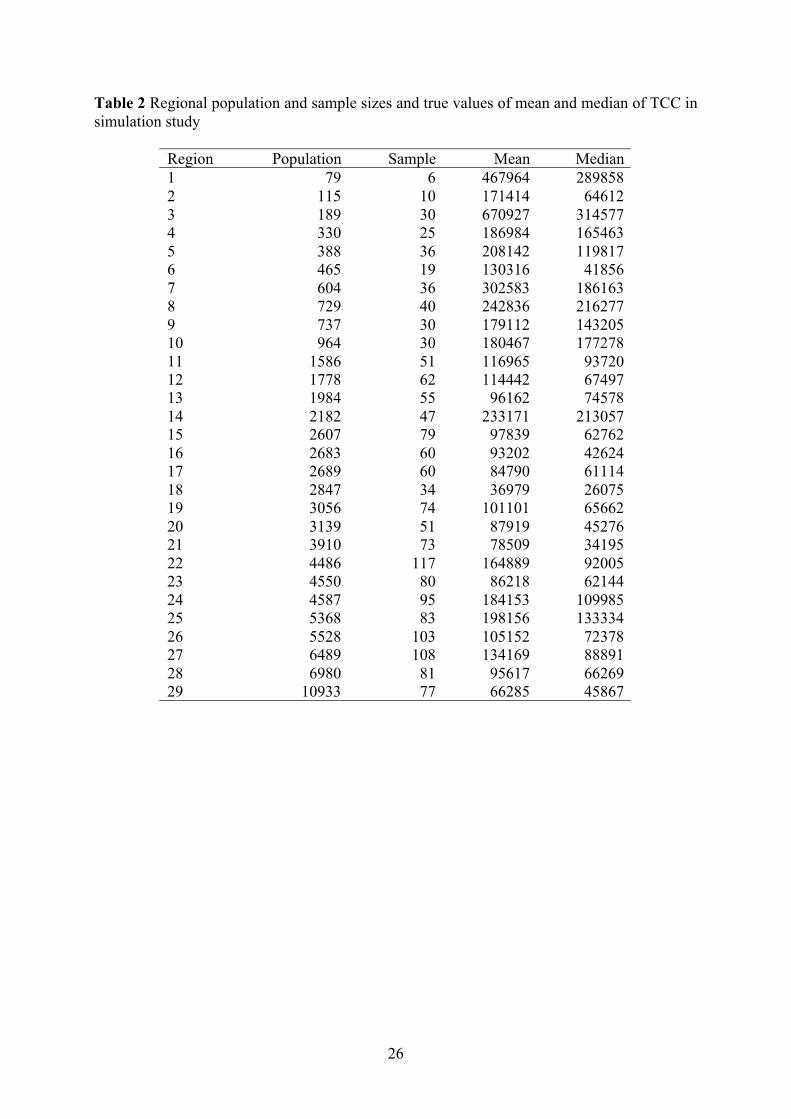
fixed to be the same as in the original sample. Table 2 shows the population and

sample size, as well as the mean and median of TCC within each region.

The same second order fixed effects specification was used by all estimation methods, defined

by the main effects and interactions for the Farmarea and SizeZone variables, with a random

slopes specification implemented by assuming a random slope for Farmarea.

The results set out in Tables 3 and 4 focus on estimation of regional means. These show that

estimation via mixed models typically leads to smaller relative biases (Table 3). However,

these smaller biases come at a cost of significantly higher variability. Consequently when we

compare relative root mean squared errors (Table 4) we see that all four methods are

20

essentially the same. The larger bias of the M-quantile approach is due to the presence of

outlying values in the dataset. Essentially, such outlying values receive small weights under

the M-quantile approach and so bias is introduced when the target of inference is the small

area mean. In contrast the smaller variation in weights under the less robust Expectile

approach means that this bias is reduced.

A very different picture emerges when we turn to estimation of regional medians, however.

Now we see that both M-quantile methods exhibit much smaller relative bias (Table 5) as well

as relative median bias (Table 6) than the methods based on application of mixed models.

Furthermore, these lower biases are accompanied by lower variances, leading to relative root

mean squared errors (Table 7) for the M-quantile methods that are around a half of those

observed for the mixed model-based methods.

Finally, in Table 8 we show the coverage performances of confidence intervals for the

regional means based on M-quantile and Expectile estimates and the MSE estimator (10).

Here we see that the larger design-biases of the M-quantile method (see Table 3) lead to

poorer coverage than the Expectile method. As expected, using the population residual-based

variance estimator (8a) in (10) leads to conservative estimates of MSE. However, this

conservatism persists when we use the area residual-based variance estimator (8b) in (10),

which is somewhat surprising. Overall, provided the M-quantile method used is itself not very

biased, it seems clear that the MSE estimator (10) is generally conservative, indicating that

further research is required to identify a more accurate method of MSE estimation under M-

quantile sample weighting.

7. Concluding Remarks

In this paper we introduce M-quantile models for small area estimation. These models offer

a natural way of modeling between area variability in data without imposing prior

21

assumptions about the source of this variability. In particular, with M-quantile models there is

no need to explicitly specify the random components of the model, with inter-area differences

captured via area-specific M-quantile coefficients instead. As a consequence, the M-quantile

approach reduces the need for parametric assumptions and provides great flexibility in model

selection. In addition, estimation and outlier robust inference under these models is

straightforward. The proposed approach appears to be suitable for estimating a wide range of

parameters and our simulation results show that it is a reasonable alternative to mixed effects

models for small area estimation.

The M-quantile approach also opens new areas for research in the practical use of mixed

models. For example, the existence of hierarchical effects of a particular type may be checked

using diagnostic tests based on the M-quantile coefficients associated with this hierarchy.

Alternatively, tests for the significance or otherwise of the coefficients of the M-quantile

model may be useful in deciding on an appropriate formulation for the random part of a

mixed effects model.

An important problem in small area estimation is the impact of changing small area

geographies on the estimates. This is difficult to resolve using mixed effects models since the

random effects in these models are geography dependent, and so a change in the geography

requires new random effects to be estimated. Such problems do not arise with M-quantile

models since M-quantile coefficients are associated with individual population units and so do

not change when a new geography is introduced. This allows the corresponding M-quantile

coefficients for the new geography to be obtained by simply re-aggregating these fixed unit

level M-quantile coefficients.

As in any branch of statistics, it is important for the data analyst involved in small area

estimation to decide on an appropriate target of inference. For example, with highly skewed

distributions one might assume that the median is a more appropriate measure of central

22

tendency than the mean. In such a case, a robust approach like the M-quantile one will

outperform the mixed effects approach. If however the mean is chosen as the target of

inference, then our simulation results indicate that although in general an estimator based on a

mixed effects model will have lower bias, all approaches are close in mean squared error

terms. Nevertheless, low bias is typically a desirable property, and further research is ongoing

to modify the M-quantile approach in such situations to decrease its bias. This research will

be reported elsewhere.

Acknowledgements

The research described in this paper was carried out under grant H333250030 of the

Economic and Social Research Council.

References

Aragon, Y., et. al. (2005). Conditional ordering using nonparametric expectiles. Working

Paper M05/01, Southampton Statistical Sciences Research Institute.

Bates, D.M. and Pinheiro, J.C. (1998). Computational methods for multilevel models.

Available in PostScript or PDF formats at http://franz.stat.wisc.edu/pub/NLME/

Battese, G.E., et. al. (1988). An error component model for prediction of county crop areas

using survey and satellite data. Journal of the American Statistical Association 83, 28-36.

Breckling, J. and Chambers, R. (1988). M-quantiles. Biometrika 75, 761-71.

Chambers, R.L. (2005a). Calibrated weighting for small area estimation. Working Paper

M05/04, Southampton Statistical Sciences Research Institute.

Chambers, R.L. (2005b). What if …. Robust prediction intervals for unbalanced samples.

Working Paper M05/05, Southampton Statistical Sciences Research Institute.

23

Engel, E. (1857). Die Produktions- und Konsumverhältnisse des Königreichs Sachsen.

Zeitschrift des Statistischen Büros des Königlich Sächsischen Ministeriums des Inneren, 8,

1-54.

Fay, R.E. and Herriot, R.A. (1979). Estimation of income from small places: An application

of James-Stein procedures to census data. Journal of the American Statistical Association

74, 269-77.

He, X. (1997). Quantile curves without crossing. The American Statistician, 51, 186-92.

Henderson, C.R. (1953). Estimation of variance and covariance components, Biometrics, 9,

226-52.

Kackar, R.N. and Harville, D.A. (1981). Unbiasedness of two-stage estimation and prediction

procedures for mixed linear models. Communications in Statistics, Series A, 10, 1249-61.

Koenker, R. and Bassett, G. (1978). Regression quantiles. Econometrica, 46, 33-50.

Koneker, R. (1984). A note on L-estimators for linear models. Statistics and Probability

Letters, 2, 323-25

Koenker R. and D’Orey, V. (1987). Computing regression quantiles, Applied Statistics, 36,

383-93.

Koenker, R. and Hallock, K.F. (2001). Quantile regression: An introduction, Journal of

Economic Perspectives, 51, 143-56.

Kokic, P. et. al. (1997). A measure of production performance, Journal of Business and

Economic Statistics, 15, 445-51.

Mosteller, F. and Tukey, J.W. (1977). Data Analysis and Regression. A Secondary Course in

Statistics, Reading, MA: Addison-Wesley.

Newey, W.K. and Powell, J.L. (1987). Asymmetric least squares estimation and testing,

Econometrica, 55, 819-47.

24

R Development Core Team (2004). R: A language and environment for statistical computing.

R Foundation for Statistical Computing, Vienna, Austria. URL: http://www.R-project.org.

Rao, J.N.K. (2003). Small Area Estimation. New York: Wiley.

Richardson, A.M. and Welsh, A.H. (1996). Covariate screening in mixed linear models,

Journal of Multivariate Analysis, 58, 27-54.

Royall, R.M. and Cumberland, W.G. (1978). Variance estimation in finite population

sampling. Journal of the American Statistical Association, 73, 351 - 58.

Venables, W.N. and Ripley, B.D. (2002). Modern Applied Statistics with S. New York:

Springer.

25

Table 1 Simulation results for two level linear populations, averaged over 30 small areas.

(θ,ρ)(0,0) (1,0) (1,0.8) (1,-0.8)

Target Small area means

True Values 311.55 306.59 303.33 309.01

Bias Random Intercept -0.0146 -0.0235 0.0531 0.0383

Random Slope -0.0153 -0.0216 0.0517 0.0378

M-quantile -0.0099 -0.0262 0.0434 0.0313

Expectile -0.0144 -0.0191 0.0496 0.0344

MSE Random Intercept 36.6642 37.0088 37.0627 36.8944

Random Slope 37.4859 37.8589 37.8553 37.7638

M-quantile 38.3347 38.7716 38.7370 38.6626

Expectile 38.9502 39.3084 39.3792 39.2130

Target Small area medians

True Values 304.91 268.01 273.27 271.37

Bias Random Intercept -0.0198 -0.0586 0.0566 0.0441

Random Slope -0.0185 -0.0575 0.0576 0.0442

M-quantile -0.0104 0.0008 0.0584 0.0582

Expectile -0.0172 -0.0459 0.0495 0.0489

MSE Random Intercept 37.8152 38.1643 37.6615 38.4915

Random Slope 38.5907 39.0929 38.4932 39.3696

M-quantile 78.8197 79.3346 79.1432 78.8080

Expectile 40.3005 40.1914 39.7312 40.3368

26

Table 2 Regional population and sample sizes and true values of mean and median of TCC in

simulation study

Region Population Sample Mean Median

1 79 6 467964 289858

2 115 10 171414 64612

3 189 30 670927 314577

4 330 25 186984 165463

5 388 36 208142 119817

6 465 19 130316 41856

7 604 36 302583 186163

8 729 40 242836 216277

9 737 30 179112 143205

10 964 30 180467 177278

11 1586 51 116965 93720

12 1778 62 114442 67497

13 1984 55 96162 74578

14 2182 47 233171 213057

15 2607 79 97839 62762

16 2683 60 93202 42624

17 2689 60 84790 61114

18 2847 34 36979 26075

19 3056 74 101101 65662

20 3139 51 87919 45276

21 3910 73 78509 34195

22 4486 117 164889 92005

23 4550 80 86218 62144

24 4587 95 184153 109985

25 5368 83 198156 133334

26 5528 103 105152 72378

27 6489 108 134169 88891

28 6980 81 95617 66269

29 10933 77 66285 45867

27

Table 3 Relative biases of estimates of regional means of TCC in simulation study. Regions

ordered by increasing population size.

Region Random

Intercept

Random

Slope

M-quantile Expectile

1 3.57 -6.99 -14.12 -0.14

2 12.12 15.50 -22.20 -12.16

3 -4.77 0.64 -29.13 -14.65

4 30.66 10.21 6.81 15.91

5 9.15 5.70 -12.90 -0.20

6 50.54 22.81 -21.31 0.73

7 1.94 -2.69 -10.71 2.95

8 -10.51 -7.72 -16.61 -15.85

9 -7.10 4.93 -22.90 -21.38

10 -4.59 -2.45 -14.20 -10.95

11 15.36 14.36 2.84 12.30

12 -7.87 -8.72 -31.51 -24.87

13 7.08 8.19 -12.27 -5.31

14 1.08 2.45 -10.06 -3.77

15 2.10 0.09 -14.56 -7.18

16 -6.21 -7.02 -30.97 -25.09

17 4.83 5.40 -14.89 -8.70

18 25.62 32.44 10.87 18.93

19 -2.55 -2.54 -21.29 -14.96

20 12.35 12.77 -4.43 12.35

21 -10.49 -8.67 -26.39 -20.14

22 4.55 1.00 -15.87 -3.06

23 6.26 6.34 -8.20 -1.59

24 -7.78 -5.44 -31.29 -25.13

25 -6.33 -3.01 -29.46 -24.31

26 2.44 3.53 -15.17 -9.10

27 -2.72 -4.25 -23.76 -18.50

28 -0.07 0.65 -16.18 -9.12

29 -1.60 -2.20 -19.05 -13.48

Mean 4.04 2.94 -16.17 -7.81

Median 1.94 0.65 -15.87 -9.10

28

Table 4 Relative root mean squared errors of estimates of regional means of TCC in

simulation study. Regions ordered by increasing population size.

Region Random

Intercept

Random

Slope

M-quantile Expectile

1 19.63 31.41 24.32 24.36

2 22.13 41.71 31.89 25.64

3 21.52 28.72 30.88 23.48

4 36.66 20.71 15.51 20.98

5 17.43 15.03 14.81 10.04

6 98.51 57.86 37.38 40.10

7 17.84 26.41 13.05 16.10

8 14.21 12.41 17.67 16.86

9 14.43 16.43 23.92 24.09

10 10.37 10.04 15.88 13.72

11 21.21 21.78 7.02 13.74

12 15.24 14.40 31.90 25.39

13 15.51 16.16 13.19 7.60

14 11.45 19.56 13.74 11.43

15 18.07 17.18 15.44 9.33

16 11.27 11.93 31.23 25.43

17 16.24 16.15 15.56 10.51

18 34.91 43.88 14.21 21.58

19 7.72 8.27 21.78 15.74

20 20.55 21.99 12.65 18.27

21 29.85 28.47 26.74 21.35

22 12.20 9.59 17.18 12.12

23 17.54 17.68 9.11 4.75

24 17.05 18.49 31.50 25.43

25 11.13 9.81 29.62 24.54

26 11.65 11.79 15.58 9.83

27 8.98 11.28 24.07 19.05

28 7.68 7.42 16.81 10.32

29 7.46 7.02 19.41 14.04

Mean 19.60 19.78 20.41 17.79

Median 16.24 16.43 17.18 16.86

29

Table 5 Relative biases of estimates of regional medians of TCC in simulation study. Regions

ordered by increasing population size.

Region Random

Intercept

Random

Slope

M-quantile Expectile

1 44.54 33.01 35.17 37.87

2 168.74 180.47 10.67 -0.81

3 51.74 54.59 7.91 12.00

4 35.02 18.64 -10.48 -11.78

5 -9.05 9.27 -11.01 -20.95

6 -4.16 36.28 -0.27 -0.67

7 5.06 12.61 8.38 5.83

8 -3.73 -4.30 -5.88 -3.96

9 10.89 11.15 -12.21 -14.21

10 -14.56 -14.19 -22.31 -17.61

11 71.73 62.21 39.27 40.21

12 35.05 22.09 6.48 6.42

13 15.18 18.79 -12.48 -13.63

14 7.99 7.23 1.11 1.59

15 4.32 4.51 -3.92 -4.77

16 58.15 50.72 6.36 5.01

17 28.28 29.52 -0.51 -0.62

18 17.82 34.61 -15.52 -16.91

19 30.91 29.72 6.69 8.10

20 68.38 77.64 59.60 60.68

21 55.26 67.53 10.40 11.59

22 94.74 86.35 53.58 52.79

23 7.06 15.12 -9.14 -10.16

24 28.40 23.99 -3.50 -6.83

25 29.56 25.51 7.59 2.51

26 30.50 31.67 13.29 10.68

27 15.47 9.65 -11.11 -11.77

28 8.01 7.08 -1.64 -2.74

29 6.56 6.37 -10.53 -11.15

Mean 30.96 32.68 4.69 3.68

Median 28.30 24.00 -0.27 -0.67

30

Table 6 Relative median biases of estimates of regional medians of TCC in simulation study.

Regions ordered by increasing population size.

Region Random

Intercept

Random

Slope

M-quantile Expectile

1 44.78 29.46 10.68 11.92

2 166.14 183.77 -7.63 -30.63

3 50.76 50.38 0.13 8.18

4 33.63 16.03 -17.37 -17.53

5 -5.74 7.96 -13.78 -24.66

6 3.79 28.73 -0.51 0.26

7 3.53 8.90 8.05 3.55

8 -3.31 -4.26 -6.78 -5.53

9 9.38 9.54 -8.46 -12.04

10 -15.41 -14.94 -21.61 -18.77

11 72.19 56.07 35.84 34.91

12 32.86 21.65 4.79 3.70

13 9.99 14.30 -12.38 -12.93

14 9.65 7.56 0.66 -1.32

15 -4.62 -2.04 -3.80 -5.06

16 56.15 48.25 3.89 4.03

17 21.93 24.33 0.02 0.02

18 16.83 33.17 -13.85 -15.64

19 30.42 29.17 5.10 6.91

20 65.96 76.38 54.86 54.78

21 38.13 52.32 8.94 9.81

22 104.76 84.31 54.32 53.32

23 0.49 8.25 -9.70 -11.52

24 24.47 17.88 -4.08 -7.01

25 29.24 25.80 7.46 2.42

26 27.33 28.89 13.82 11.66

27 13.34 8.48 -12.51 -13.99

28 7.02 6.47 -1.42 -2.46

29 5.55 5.30 -11.11 -11.61

Mean 29.28 29.73 2.19 0.51

Median 21.90 21.60 -0.51 -1.32

31

Table 7 Relative root mean squared errors of estimates of regional medians of TCC in

simulation study. Regions ordered by increasing population size.

Region Random

Intercept

Random

Slope

M-quantile Expectile

1 52.16 54.11 75.28 75.19

2 182.04 209.03 68.38 76.09

3 56.07 62.07 19.53 21.49

4 43.16 28.77 24.66 27.89

5 27.30 19.25 19.26 27.05

6 58.83 59.45 5.24 7.10

7 24.30 24.03 11.28 12.78

8 10.88 10.93 12.65 12.27

9 17.87 17.10 20.87 22.86

10 17.68 17.70 25.97 21.42

11 76.12 67.71 44.13 46.27

12 40.16 27.27 17.48 16.54

13 25.70 27.09 15.17 16.25

14 13.90 13.67 15.20 14.60

15 34.73 32.65 11.57 12.00

16 61.45 53.76 15.61 13.97

17 37.90 38.22 6.70 7.85

18 37.97 53.96 23.36 24.26

19 33.09 31.76 11.42 13.16

20 80.66 85.74 67.38 68.66

21 92.25 96.63 17.12 18.34

22 104.68 90.06 56.77 59.34

23 31.01 31.70 12.70 14.03

24 36.82 35.90 8.46 11.56

25 33.30 28.18 11.60 10.59

26 35.50 36.00 14.95 13.78

27 21.48 19.42 12.46 13.44

28 13.78 12.24 5.60 6.09

29 11.96 10.29 11.72 12.18

Mean 45.27 44.65 22.85 24.04

Median 35.50 31.76 15.20 14.60

32

Table 8 Coverage rates of “2 sigma” confidence intervals for regional population means of

TCC. Intervals are defined by the M-quantile and Expectile estimates plus or minus twice

their corresponding standard errors using either (8a) (“Population Residuals”) or (8b) (“Area

Residuals”) in (10). Regions ordered by increasing population size.

Area Residuals Population ResidualsRegion

M-quantile Expectile M-quantile Expectile

1 0.56 0.84 0.55 0.88

2 1.00 0.97 1.00 0.98

3 0.46 0.79 0.40 0.78

4 0.98 1.00 0.99 1.00

5 0.93 1.00 0.96 1.00

6 0.94 0.99 0.95 1.00

7 0.82 0.99 0.75 0.99

8 0.99 1.00 0.99 1.00

9 0.47 1.00 0.58 1.00

10 0.99 1.00 0.99 1.00

11 1.00 1.00 1.00 1.00

12 0.21 0.65 0.17 0.67

13 1.00 1.00 1.00 1.00

14 0.96 1.00 0.94 1.00

15 0.60 0.94 0.56 0.96

16 0.03 0.56 0.03 0.78

17 0.52 1.00 0.63 1.00

18 1.00 1.00 1.00 1.00

19 1.00 1.00 1.00 1.00

20 1.00 1.00 1.00 1.00

21 0.96 1.00 0.99 1.00

22 1.00 1.00 1.00 1.00

23 1.00 1.00 1.00 1.00

24 0.06 0.59 0.06 0.76

25 0.26 0.98 0.19 0.99

26 0.99 1.00 1.00 1.00

27 0.77 1.00 0.68 0.99

28 1.00 1.00 1.00 1.00

29 1.00 1.00 1.00 1.00

Mean 0.77 0.94 0.77 0.96

Median 0.94 1.00 0.99 1.00