source activity correlation effects on lcmv beamformers in a

Hindawi Publishing CorporationComputational and Mathematical Methods in MedicineVolume 2012, Article ID 190513, 8 pagesdoi:10.1155/2012/190513

Research Article

Source Activity Correlation Effects on LCMV Beamformers ina Realistic Measurement Environment

Paolo Belardinelli,1 Erick Ortiz,1 and Christoph Braun1, 2, 3

1 MEG Center, University of Tubingen, Otfried Mueller Street 47, 72076 Tubingen, Germany2 CIMeC, Center of Mind/Brain Sciences, University of Trento, Via Delle Regole 101, 38123 Mattarello, Italy3 DiSCoF, Department of Cognitive and Educational Sciences, University of Trento, Corso Bettini no. 31,38068 Rovereto, Italy

Correspondence should be addressed to Paolo Belardinelli, [email protected]

Received 17 November 2011; Revised 1 February 2012; Accepted 9 February 2012

Academic Editor: Luca Faes

Copyright © 2012 Paolo Belardinelli et al. This is an open access article distributed under the Creative Commons AttributionLicense, which permits unrestricted use, distribution, and reproduction in any medium, provided the original work is properlycited.

In EEG and MEG studies on brain functional connectivity and source interactions can be performed at sensor or source level.Beamformers are well-established source-localization tools for MEG/EEG signals, being employed in source connectivity studiesboth in time and frequency domain. However, it has been demonstrated that beamformers suffer from a localization bias due tocorrelation between source time courses. This phenomenon has been ascertained by means of theoretical proofs and simulations.Nonetheless, the impact of correlated sources on localization outputs with real data has been disputed for a long time. In thispaper, by means of a phantom, we address the correlation issue in a realistic MEG environment. Localization performances in thepresence of simultaneously active sources are studied as a function of correlation degree and distance between sources. A linearconstrained minimum variance (LCMV) beamformer is applied to the oscillating signals generated by the current dipoles withinthe phantom. Results show that high correlation affects mostly dipoles placed at small distances (1, 5 centimeters). In this case thesources merge. If the dipoles lie 3 centimeters apart, the beamformer localization detects attenuated power amplitudes and blurredsources as the correlation level raises.

1. Introduction

MEG and EEG provide noninvasive imaging over thewhole brain with an excellent temporal resolution. Thehigh temporal resolution qualifies these methods for thestudy of functional connectivity based on correlated activity.Over the last three decades, several algorithms have beendeveloped for brain source localization [1]. Besides recentBayesian approaches which employ iterative (and there-fore computationally demanding) inversion schemes [2–4],beamformers [5, 6] still hold as one of the most reliableinversion schemes for source localization both in time andfrequency domain [7–15]. Beamformers are data-dependentspatial filters. In order to pass from sensor signals to brainsource activity, they employ filters which rely on the signalcovariance (time domain) or the cross-spectrum densitymatrix (frequency domain). Moreover, beamformers assume

uncorrelated source timecourses. The covariance estimationis therefore forced to be diagonal. This may induce a biasboth on location and intensity of the detected sources [16].Some findings have shown that this assumption produces noevident bias with certain data sets. On the other hand, otherstudies have demonstrated that it may induce relevant biaseswhen the level of correlation between sources and the signal-to-noise Ratio are high [17, 18]. A dual-core beamformerthat takes into account the correlation effects between twosources has been implemented by Brookes et al. [19]. How-ever, this modified beamformer implies the use of a prioriinformation which is not always available. The correlationeffects are particularly disruptive when analyzing brain-induced or spontaneous activity in the frequency domain. Infact, some possible remedies for modeling correlation effectshave been proposed for the study of evoked potential in thetime domain [20, 21]. However, these approaches based on

2 Computational and Mathematical Methods in Medicine

Bayesian theory call for a strong assumption about what is“signal” and what is “noise/spontaneous activity” within thetime span of our data. This is clearly not possible in presenceof data generated by spontaneous or induced brain activity.

In this paper, we have set true current dipoles withina phantom and measured the MEG signals generated bysources with various levels of mutual correlation locatedat different depths and mutual distances. The goal of thepaper was to elucidate how correlation affects beamformerresults in a realistic measurement environment. For thisaim, we have localized the oscillating sources both in timeand frequency domain by means of a linear constrainedminimum variance (LCMV) beamformer. Since the local-ization results appeared extremely similar, we focused onthe frequency domain which is a power implementation ofdynamic imaging of coherent sources (DICS) [10].

2. Materials and Methods

2.1. Forward Solution

2.1.1. Phantom Description. In this experiment the CTFphantom model PN900-0017 was employed. This phantomconsists of a 65 mm acrylic sphere, filled with saline water at0.8% concentration, and based on an empty vertical acrylictube. This tool emulates the brain volume conductor and theconductive medium around it. The brain current dipoles aresimulated by a twisted pair of isolated wires, with open ends,encased in a glass tube. These tubes enter the sphere from theinferior part through a grid of holes that allows the dipoles tobe located at different positions on the horizontal plane.

2.1.2. Head Coordinate System. To define the head coordi-nate system, three coils are vertically located at standardpositions on the surface of the phantom sphere. The threelocations loosely correspond to the fiducial points commonlyused with human subjects: nasion (NAS), left periauricularpoint (LPA), and right periauricular point (RPA). The originis considered the midpoint between RPA and LPA. All ofthe three points lie on the central horizontal plane of thesphere. The X axis points directly to NAS, and the Y axis isorthogonal to it, pointing approximately towards LPA. The Zaxis is orthogonal to the XY plane, pointing at the top of thesphere.

In order to define the head localization, the three smallcoils (NAS, LPA, and RPA) generate a magnetic dipolesignal. The center of the magnetic dipole coil is 50 mmabove the plane containing the center of all three headlocalization coils. The dipole coil is an 11-turn single-layerair core solenoid wound on a 1.6 mm diameter mandrill.The magnetic field generated by a coil is different from themagnetic field generated by a current dipole. As a result,a different localization calculation is used for the magneticdipole phantom.

2.1.3. Dipole Locations. Two different dipole configurationswere considered: one with two parallel dipoles (#1 and #2)

placed on the same coronal plane in the two different hemi-spheres (Figure 1). The dipoles had different distances fromthe surface (2 and 3 cm, resp.). The distance between thedipoles was 3 centimeters. In the second configuration thetwo dipoles (#1 and #3) were placed in the left hemisphere ata slightly height (2 and 0.5 cm from the surface, resp.), withdipole #3 more external with respect to #1. Their distance inthis case was 1.5 centimeters.

2.1.4. Simulated Electric Signals. The dipoles’ electric signalswere divided into 200 epochs (100 epochs with oscillatingdipoles, 100 with inactive ones) with a length of 0.8seconds. The time courses were generated synthetically froma frequency distribution centered at 10 Hz, controlled for thedesired correlation levels, and then commuted into electricsignals by means of a digital to analog converter (DAC).

A computer with a DAC board Adlink ACL-6126 wasused, with one independent channel per dipole, with alter-nating current output in a range of ± 5 μA. Since we placedone dipole (#3, Figure 1) on a location which can be roughlyassociated to the sensorimotor region, a typical range ofelectrical activity for somatosensory responses was used [22].Our DAC sampling rate was 200 Hz, the MEG sampling ratewas 293 Hz. The DAC board employed for our experimenthas bipolar outputs, with a common ground. Thus, while thevoltage output was bipolar, the pair was not allowed to float.

Under the conditions mentioned above, the ideal dipolecurrent drivers are optically isolated current sources; how-ever, in the absence of this option, the best solution was(1) to use a DAC with differential outputs (range: ±5 V)with a 1 Mohm resistor attached to both the positive andnegative outputs, and (2) to ensure adequate separation(1.5 or 3 cm) between the dipole pairs, compared to thedipole length (3 mm). Part (1) of the solution ensures aknown and matched value for the current in each cableof the dipole pair, and part (2) keeps the current betweenthe pairs one order of magnitude lower than in eachdipole.

2.1.5. Synthetic Time-Course Generation. For each time sam-ple, an instantaneous frequency was drawn from a Gaussiandistribution centered on a 10 Hz frequency: N(10 Hz, 3 Hz).The final time course consisted of the cumulative sum of suchinstantaneous frequencies, with a random initial phase. Thedipole time courses were controlled either for low (0.15 ±0.05) medium (0.55± 0.05) or high (0.95± 0.05) correlation(Figure 2).

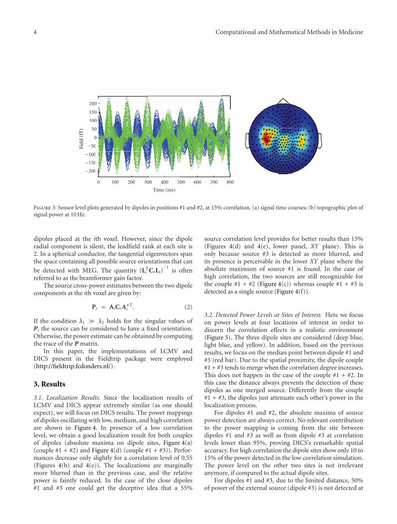
In Figure 3 we show a plot of sensor data in the timedomain and a sensor-power plot of Fourier transformed dataat the frequency of interest of 10 Hz.

2.2. Spatial Filters. Since the focus of our work is to quantifythe influence of correlation in the localization accuracy ofdipoles with known locations, the choice of source mappingstrategy was a voxel-wise spatial filter, named beamformer.Parameters for these spatial filters depend both on theforward model chosen (source distribution and a volumeconductor model) and the data.

Computational and Mathematical Methods in Medicine 3

Figure 1: Setting of the three dipoles within the coverless phantom.Squares have a 5 mm side. In the left upper corner, the completesetup is shown.

2.2.1. Forward Model. A three-dimensional grid with 5 mmstep was employed for source analysis, bounded by asphere of 65 mm radius centered at the origin. At eachgrid point (voxel), the full rank-3 leadfield is calculated,and subsequently reduced to rank-2, since in a sphericalconductor model the radial component is zero [23]. Thevolume conductor model is a sphere with a radius of 7 cm.

2.2.2. Linear Constrained Minimum Variance (LCMV) Beam-former. Linear Constrained Minimum Variance beamform-ers are widely employed both in time and frequency domain[9, 10]. As a first step, the 100 active epochs and the 100inactive ones are Fourier transformed and then averaged.DICS source power mapping procedure was applied to thedata to both averages. Then, the output of the silent averagewas used as a baseline. The active average was contrasted tothe baseline.

LCMV and DICS consist in the following procedure: afilter matrix A is employed in a linear transformation fromthe sensor level to the brain space. A filters the source activity(in a given frequency band or time window) at the ith voxel(grid point) with unit gain while suppressing contributionfrom the other voxels. The filter depends on the data bymeans of the covariance C(t) (LCMV, time domain) or thecross spectral density (CSD) C(f ) (DICS, frequency domain).Since the two domains are dual, we will define both matricesas C in the following description of the filtering procedure.The minimization problem which yields A has the followingsolution:

Ai =(

LTi CrLi

)−1LTi C−1

r , (1)

where Cr = C + αI and α is a regularization parameter.In our case α = 15%, the time window of interest t wasthe entire epoch and f = 10 ± 3 Hz so that most ofthe signal information content was considered. L is theleadfield matrix. The columns of L contain the solutionof the forward problem for three orthogonal unit current

0 200 400 600 800−1

−0.5

0

0.5

1Corr. coef. = 0.15

Time (ms)

Nor

mal

ized

am

plit

ude

(a)

Nor

mal

ized

am

plit

ude

0 200 400 600 800−1

−0.5

0

0.5

1Corr. coef. = 0.55

Time (ms)

(b)

Nor

mal

ized

am

plit

ude

0 200 400 600 800 −1

−0.5

0

0.5

1Corr. coef. = 0.95

Time (ms)

(c)

Figure 2: Time-courses for three different levels of correlation.Dashed and solid curves represent the dipole activities on the twosource locations. Due to the addition of Gaussian noise, the signalsdiverge slightly from sine waves. Their phase synchrony grows ascorrelation increases.


0 100 200 300 400 500 600 700 800

−200

−150

−100

−50

0 100 200 30

0

−200

50

100

150

200

Time (ms)

Fiel

d (f

T)

00 600 700

−150

−100

−50

0

50

100

150

200

Fiel

d (f

T)

800

Figure 3: Sensor level plots generated by dipoles in positions #1 and #2, at 15% correlation. (a) signal time courses; (b) topographic plot ofsignal power at 10 Hz.

dipoles placed at the ith voxel. However, since the dipoleradial component is silent, the leadfield rank at each site is2. In a spherical conductor, the tangential eigenvectors spanthe space containing all possible source orientations that can

be detected with MEG. The quantity (LTi CrLi)

−1is often

referred to as the beamformer gain factor.The source cross-power estimates between the two dipole

components at the ith voxel are given by:

Pi = AiCrA∗Ti . (2)

If the condition λ1 � λ2 holds for the singular values ofP, the source can be considered to have a fixed orientation.Otherwise, the power estimate can be obtained by computingthe trace of the P matrix.

In this paper, the implementations of LCMV andDICS present in the Fieldtrip package were employed(http://fieldtrip.fcdonders.nl/).

3. Results

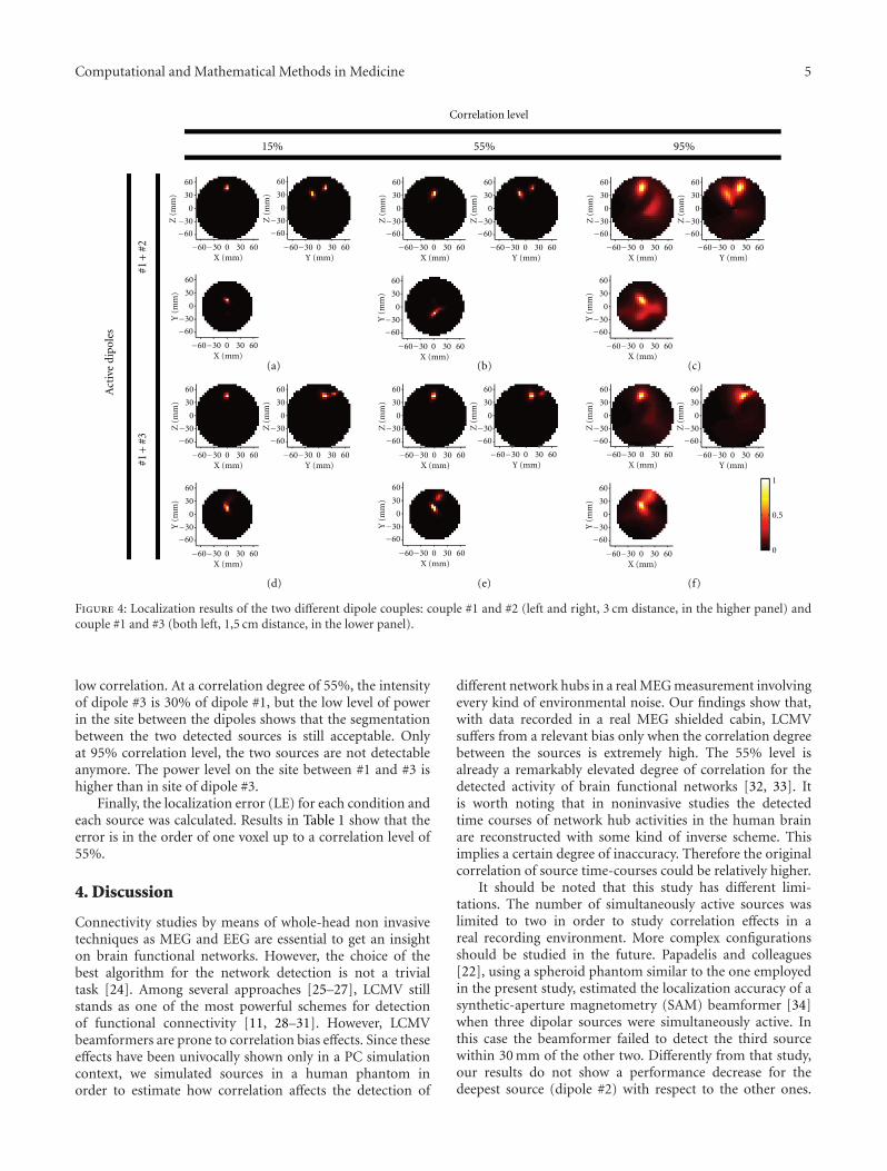
3.1. Localization Results. Since the localization results ofLCMV and DICS appear extremely similar (as one shouldexpect), we will focus on DICS results. The power mappingsof dipoles oscillating with low, medium, and high correlationare shown in Figure 4. In presence of a low correlationlevel, we obtain a good localization result for both couplesof dipoles (absolute maxima on dipole sites, Figure 4(a)(couple #1 + #2) and Figure 4(d) (couple #1 + #3)). Perfor-mances decrease only slightly for a correlation level of 0.55(Figures 4(b) and 4(e)). The localizations are marginallymore blurred than in the previous case, and the relativepower is faintly reduced. In the case of the close dipoles#1 and #3 one could get the deceptive idea that a 55%

source correlation level provides for better results than 15%(Figures 4(d) and 4(e), lower panel, XY plane). This isonly because source #3 is detected as more blurred, andits presence is perceivable in the lower XY plane where theabsolute maximum of source #1 is found. In the case ofhigh correlation, the two sources are still recognizable forthe couple #1 + #2 (Figure 4(c)) whereas couple #1 + #3 isdetected as a single source (Figure 4(f)).

3.2. Detected Power Levels at Sites of Interest. Here we focuson power levels at four locations of interest in order todiscern the correlation effects in a realistic environment(Figure 5). The three dipole sites are considered (deep blue,light blue, and yellow). In addition, based on the previousresults, we focus on the median point between dipole #1 and#3 (red bar). Due to the spatial proximity, the dipole couple#1 + #3 tends to merge when the correlation degree increases.This does not happen in the case of the couple #1 + #2. Inthis case the distance always prevents the detection of thesedipoles as one merged source. Differently from the couple#1 + #3, the dipoles just attenuate each other’s power in thelocalization process.

For dipoles #1 and #2, the absolute maxima of sourcepower detection are always correct. No relevant contributionto the power mapping is coming from the site betweendipoles #1 and #3 as well as from dipole #3 at correlationlevels lower than 95%, proving DICS’s remarkable spatialaccuracy. For high correlation the dipole sites show only 10 to15% of the power detected in the low correlation simulation.The power level on the other two sites is not irrelevantanymore, if compared to the actual dipole sites.

For dipoles #1 and #3, due to the limited distance, 50%of power of the external source (dipole #3) is not detected at


60

60

30

30

0

0

−30

−30

−60

−60

X (mm)

Z (

mm

)

60

60

30

30

0

0

−30

−30

−60

−60

Y (mm)Z

(m

m)

60

60

30

30

0

0

−30

−30

−60

−60

X (mm)

Y (

mm

)

60

60

30

30

0

0

−30

−30

−60

−60

X (mm)

Y (

mm

)

60

60

30

30

0

0

−30

−30

−60

−60

X (mm)

Z (

mm

)

60

60

30

30

0

0

−30

−30

−60

−60

Y (mm)

Z (

mm

)

60

60

30

30

0

0

−30

−30

−60

−60

X (mm)

Z (

mm

)

60

60

30

30

0

0

−30

−30

−60

−60

Y (mm)

Z (

mm

)

60

60

30

30

0

0

−30

−30

−60

−60

X (mm)

Y (

mm

)

60

60

30

30

0

0

−30

−30

−60

−60

Y (mm)

Z (

mm

)

60

60

30

30

0

0

−30

−30

−60

−60

X (mm)

Z (

mm

)

60

60

30

30

0

0

−30

−30

−60

−60

Y (mm)Z

(m

m)

60

60

30

30

0

0

−30

−30

−60

−60

X (mm)

Z (

mm

)

60

60

30

30

0

0

−30

−30

−60

−60

Y (mm)

Z (

mm

)

60

60

30

30

0

0

−30

−30

−60

−60

X (mm)

Z (

mm

)

60

60

30

30

0

0

−30

−30

−60

−60

X (mm)

Y (

mm

)

60

60

30

30

0

0

−30

−30

−60

−60

X (mm)

Y (

mm

)

1

0.5

0

60

6030

30

0

0

−30

−30

−60

−60

X (mm)

Y (

mm

)

Act

ive

dipo

les

#1+

#3#1

+#2

Correlation level

15% 55% 95%

(a) (b) (c)

(f)(e)(d)

Figure 4: Localization results of the two different dipole couples: couple #1 and #2 (left and right, 3 cm distance, in the higher panel) andcouple #1 and #3 (both left, 1,5 cm distance, in the lower panel).

low correlation. At a correlation degree of 55%, the intensityof dipole #3 is 30% of dipole #1, but the low level of powerin the site between the dipoles shows that the segmentationbetween the two detected sources is still acceptable. Onlyat 95% correlation level, the two sources are not detectableanymore. The power level on the site between #1 and #3 ishigher than in site of dipole #3.

Finally, the localization error (LE) for each condition andeach source was calculated. Results in Table 1 show that theerror is in the order of one voxel up to a correlation level of55%.

4. Discussion

Connectivity studies by means of whole-head non invasivetechniques as MEG and EEG are essential to get an insighton brain functional networks. However, the choice of thebest algorithm for the network detection is not a trivialtask [24]. Among several approaches [25–27], LCMV stillstands as one of the most powerful schemes for detectionof functional connectivity [11, 28–31]. However, LCMVbeamformers are prone to correlation bias effects. Since theseeffects have been univocally shown only in a PC simulationcontext, we simulated sources in a human phantom inorder to estimate how correlation affects the detection of

different network hubs in a real MEG measurement involvingevery kind of environmental noise. Our findings show that,with data recorded in a real MEG shielded cabin, LCMVsuffers from a relevant bias only when the correlation degreebetween the sources is extremely high. The 55% level isalready a remarkably elevated degree of correlation for thedetected activity of brain functional networks [32, 33]. Itis worth noting that in noninvasive studies the detectedtime courses of network hub activities in the human brainare reconstructed with some kind of inverse scheme. Thisimplies a certain degree of inaccuracy. Therefore the originalcorrelation of source time-courses could be relatively higher.

It should be noted that this study has different limi-tations. The number of simultaneously active sources waslimited to two in order to study correlation effects in areal recording environment. More complex configurationsshould be studied in the future. Papadelis and colleagues[22], using a spheroid phantom similar to the one employedin the present study, estimated the localization accuracy of asynthetic-aperture magnetometry (SAM) beamformer [34]when three dipolar sources were simultaneously active. Inthis case the beamformer failed to detect the third sourcewithin 30 mm of the other two. Differently from that study,our results do not show a performance decrease for thedeepest source (dipole #2) with respect to the other ones.


15 55 950

0.2

0.4

0.6

0.8

1

1.2

1.4

1.6

1.8

2

Correlation level (%)

Rel

ativ

e po

wer

Dipoles: bilateral, far (#1+#2)

Dipole #1: left

Dipole #2: right

Dipole #3: left

Mid−#1#3

Location

×108

(a)

15 55 950

0.5

1

1.5

2

2.5

3

Correlation level (%)

Rel

ativ

e po

wer

Dipoles: left side, near (#1+#3)

Dipole #1: left

Dipole #2: right

Dipole #3: left

Mid−#1#3

Location

×108

(b)

Figure 5: Plots of relative power normalized to the baseline obtained by means of DICS at four sites of interest: location of dipole #1 (deepblue), dipole #2 (light blue), and dipole #3 (yellow) and the median point between dipole #1 and #3 (red). The high relative values are asymptom of the good performance of the spatial filter.

Table 1: Localization errors (LEs) in the LCMV outputs. Results are acceptable up until a 55% level of correlation. To our surprise, results forsource #1 and source #3 (nearby sources) at 55% were slightly better than findings on the same couple of sources with 15% correlation as wellas with far sources #1 and #2 simultaneously active at same correlation level (55%). Differences were always in the order of 1 voxel (5 mm).For high correlation between sources (95%), a more relevant error is detectable for nearby sources whereas only a single local maximum isretrievable in the area between the two sources for the far ones.

Correlation level LE source #1- source #2 (mm) LE source #1- source #3 (mm)

15% S1, 5; S2, 5 S1, 5; S3, 10

55% S1, 11; S2, 9 S1, 5; S3, 7

95% S1, 15; S2, 12 Single peaks not detectable

Our data suggest that MEG should be able to localize 3 cmdeep sources under the condition of a sufficient numberof trials (i.e., sufficiently high SNR). Furthermore, the useof a spheroid phantom is not optimal for a realistic MEGsimulation. A more realistic approach should consider dif-ferent dipole orientations and time shifts of sources as well asdifferent time-course envelopes. A possible further step in thedirection of realistic conditions would be the construction ofa human-shaped phantom with different compartments for

brain, cerebrospinal fluid (CSF), skull, and scalp. This couldpotentially yield an increase in the accuracy as shown by theMEG results in [35]. The significance of precise conductivityvalues for MEG, where only one volume conductor isused, has been downplayed by several studies [35–38];the shape of the volume conductor plays a more relevantrole. The simplest, first-order head model is a sphere; ahigher-order model could potentially map more subtletiesof the head anatomy. Leahy and colleagues show that with


a realistic skull phantom and a corresponding BEM headmodel, the MEG localization errors are comparable withthe potential registration errors. Furthermore, they foundout that the localization errors induced by a locally fittedsphere are slightly larger than those generated by a BEMmodel (3.03 mm versus 3.47 mm in the localization error;6.8◦ versus 7.7◦ in the tangential component error). Thesefindings suggest that, while generating a subject-specificvolume conductor is probably adding excessive complexity,a standard BEM model scaled to the subject (i.e., a globalrescaling transformation with 7 parameters: 6 parameters forrotation and translation and 1 for scaling) could be a faircompromise. This information can be extracted just fromthe fiducial points of the subject. We performed a briefcomparison between a spherical and a “Nolte” model [36].For the sphere, only rank-2 leadfields were used, for thereasons mentioned in the methods section; this does notnecessarily apply to the “Nolte” model. The 7-parametertransformation was then applied to a boundary elementmethod (BEM) model generated from the MRI image ofa subject’s head, and the ratio between rank-3 and rank-2 leadfields was calculated for each position on a regulargrid with 5 mm resolution. The median ratio resulted smallerthan 0.1%, indicating that most information input in themodel is nondescriptive. Only 3.7% of the sites (435 outof 11654) had a ratio larger than 1%, and less than 0.2%(20 sites) crossed a 5% threshold. This finding suggests thatthe use of a realistic phantom and a corresponding accuratemodel appears necessary only in particularly elaboratedsimulations.

The approach with real current dipoles employed in thisstudy can be further extended in the future to investigatehuman brain functional networks (resting state, acoustic,sensorimotor, etc.) comparing real and simulated (non-synthetic) data with the limitations described above. Acomparison between human networks and simulated ones atdifferent correlation levels can provide new insights both onthe physiological meaning of such human networks and onbeamformer limitations as a detection tool for connectivitystudies. In fact, the LCMV beamformer can be employed intwo simple ways in order to access brain connectivity: 1. Inthe time domain in order to reconstruct the source time-courses from different areas and in a second step to studytheir connectivity by means of different algorithms [11, 39–41]. Another possible extension of the present study is the useof DICS not just for power but also for coherence mapping.In this last case, instead of calculating the source powerestimates at the ith voxel by means of (2), the cross spectrumand coherence estimates between the tangential dipoles at thevoxels placed at r1 and r2 can be estimated for every brainvoxel [10].

Acknowledgment

The present work is supported by an award from the Centerfor Integrated Neuroscience (CIN) of Tubingen (Germany)(Pool Project no. 2010-17).

References

[1] S. Baillet, J. C. Mosher, and R. M. Leahy, “Electromagneticbrain mapping,” IEEE Signal Processing Magazine, vol. 18, no.6, pp. 14–30, 2001.

[2] K. Friston, L. Harrison, J. Daunizeau et al., “Multiple sparsepriors for the M/EEG inverse problem,” NeuroImage, vol. 39,no. 3, pp. 1104–1120, 2008.

[3] M. A. Sato, T. Yoshioka, S. Kajihara et al., “HierarchicalBayesian estimation for MEG inverse problem,” NeuroImage,vol. 23, no. 3, pp. 806–826, 2004.

[4] D. P. Wipf, J. P. Owen, H. T. Attias, K. Sekihara, and S.S. Nagarajan, “Robust Bayesian estimation of the location,orientation, and time course of multiple correlated neuralsources using MEG,” NeuroImage, vol. 49, no. 1, pp. 641–655,2010.

[5] M. D. Zoltowski, “On the performance analysis of the MVDRbeamformer in the presence of correlated interference,” IEEETransactions on Acoustics, Speech, and Signal Processing, vol. 36,no. 6, pp. 945–947, 1988.

[6] B. D. Van Veen, W. Van Drongelen, M. Yuchtman, and A.Suzuki, “Localization of brain electrical activity via linearlyconstrained minimum variance spatial filtering,” IEEE Trans-actions on Biomedical Engineering, vol. 44, no. 9, pp. 867–880,1997.

[7] G. R. Barnes and A. Hillebrand, “Statistical flattening of MEGbeamformer images,” Human Brain Mapping, vol. 18, no. 1,pp. 1–12, 2003.

[8] P. Belardinelli, L. Ciancetta, M. Staudt et al., “Cerebro-muscular and cerebro-cerebral coherence in patients with pre-and perinatally acquired unilateral brain lesions,” NeuroImage,vol. 37, no. 4, pp. 1301–1314, 2007.

[9] D. Cheyne, A. C. Bostan, W. Gaetz, and E. W. Pang,“Event-related beamforming: a robust method for presurgicalfunctional mapping using MEG,” Clinical Neurophysiology,vol. 118, no. 8, pp. 1691–1704, 2007.

[10] J. Gross, J. Kujala, M. Hamalainen, L. Timmermann, A.Schnitzler, and R. Salmelin, “Dynamic imaging of coherentsources: studying neural interactions in the human brain,”Proceedings of the National Academy of Sciences of the UnitedStates of America, vol. 98, no. 2, pp. 694–699, 2001.

[11] J. Gross, L. Timmermann, J. Kujala et al., “The neural basisof intermittent motor control in humans,” Proceedings of theNational Academy of Sciences of the United States of America,vol. 99, no. 4, pp. 2299–2302, 2002.

[12] S. D. Hall, I. E. Holliday, A. Hillebrand et al., “The missinglink: analogous human and primate cortical gamma oscilla-tions,” NeuroImage, vol. 26, no. 1, pp. 13–17, 2005.

[13] N. Hoogenboom, J. M. Schoffelen, R. Oostenveld, L. M.Parkes, and P. Fries, “Localizing human visual gamma-bandactivity in frequency, time and space,” NeuroImage, vol. 29, no.3, pp. 764–773, 2006.

[14] H. B. Hui, D. Pantazis, S. L. Bressler, and R. M. Leahy,“Identifying true cortical interactions in MEG using thenulling beamformer,” NeuroImage, vol. 49, no. 4, pp. 3161–3174, 2010.

[15] V. Litvak, A. Eusebio, A. Jha et al., “Optimized beamformingfor simultaneous MEG and intracranial local field potentialrecordings in deep brain stimulation patients,” NeuroImage,vol. 50, no. 4, pp. 1578–1588, 2010.

[16] K. Sekihara, S. S. Nagarajan, D. Poeppel, and A. Marantz,“Performance of an MEG adaptive-beamformer technique inthe presence of correlated neural activities: effects on signalintensity and time-course estimates,” IEEE Transactions onBiomedical Engineering, vol. 49, no. 12, pp. 1534–1546, 2002.


[17] K. Sekihara, S. S. Nagarajan, D. Poeppel, and A. Marantz,“Performance of an MEG adaptive-beamformer source recon-struction technique in the presence of additive low-rankinterference,” IEEE Transactions on Biomedical Engineering,vol. 51, no. 1, pp. 90–99, 2004.

[18] D. Wipf and S. Nagarajan, “Beamforming using the relevancevector machine,” in Proceedings of the 24th InternationalConference on Machine Learning (ICML ’07), pp. 1023–1030,June 2007.

[19] M. J. Brookes, C. M. Stevenson, G. R. Barnes et al., “Beam-former reconstruction of correlated sources using a modifiedsource model,” NeuroImage, vol. 34, no. 4, pp. 1454–1465,2007.

[20] J. M. Zumer, H. T. Attias, K. Sekihara, and S. S. Nagarajan,“A probabilistic algorithm integrating source localization andnoise suppression for MEG and EEG data,” NeuroImage, vol.37, no. 1, pp. 102–115, 2007.

[21] A. Dogandzic and A. Nehorai, “Estimating evoked dipoleresponses in unknown spatially correlated noise withEEG/MEG arrays,” IEEE Transactions on Signal Processing, vol.48, no. 1, pp. 13–25, 2000.

[22] C. Papadelis, V. Poghosyan, P. B. C. Fenwick, and A. A.Ioannides, “MEG’s ability to localise accurately weak transientneural sources,” Clinical Neurophysiology, vol. 120, no. 11, pp.1958–1970, 2009.

[23] J. Sarvas, “Basic mathematical and electromagnetic conceptsof the biomagnetic inverse problem,” Physics in Medicine andBiology, vol. 32, no. 1, article 11, 1987.

[24] J. M. Schoffelen and J. Gross, “Source connectivity analysiswith MEG and EEG,” Human Brain Mapping, vol. 30, no. 6,pp. 1857–1865, 2009.

[25] K. J. Friston, L. Harrison, and W. Penny, “Dynamic causalmodelling,” NeuroImage, vol. 19, no. 4, pp. 1273–1302, 2003.

[26] K. Jerbi, J. P. Lachaux, K. N’Diaye et al., “Coherent neuralrepresentation of hand speed in humans revealed by MEGimaging,” Proceedings of the National Academy of Sciences ofthe United States of America, vol. 104, no. 18, pp. 7676–7681,2007.

[27] G. Nolte, O. Bai, L. Wheaton, Z. Mari, S. Vorbach, and M. Hal-lett, “Identifying true brain interaction from EEG data usingthe imaginary part of coherency,” Clinical Neurophysiology,vol. 115, no. 10, pp. 2292–2307, 2004.

[28] P. Fries, “A mechanism for cognitive dynamics: neuronal com-munication through neuronal coherence,” Trends in CognitiveSciences, vol. 9, no. 10, pp. 474–480, 2005.

[29] M. Liljestrom, J. Kujala, O. Jensen, and R. Salmelin, “Neuro-magnetic localization of rhythmic activity in the human brain:a comparison of three methods,” NeuroImage, vol. 25, no. 3,pp. 734–745, 2005.

[30] A. Schnitzler and J. Gross, “Normal and pathological oscil-latory communication in the brain,” Nature Reviews Neuro-science, vol. 6, no. 4, pp. 285–296, 2005.

[31] J. M. Schoffelen, R. Oostenveld, and P. Fries, “Neuronal coher-ence as a mechanism of effective corticospinal interaction,”Science, vol. 308, no. 5718, pp. 111–113, 2005.

[32] F. De Pasquale, S. Della Penna, A. Z. Snyder et al., “Temporaldynamics of spontaneous MEG activity in brain networks,”Proceedings of the National Academy of Sciences of the UnitedStates of America, vol. 107, no. 13, pp. 6040–6045, 2010.

[33] D. Mantini, M. G. Perrucci, C. Del Gratta, G. L. Romani, andM. Corbetta, “Electrophysiological signatures of resting statenetworks in the human brain,” Proceedings of the NationalAcademy of Sciences of the United States of America, vol. 104,no. 32, pp. 13170–13175, 2007.

[34] S. E. Robinson and J. Vrba, “Functional neuroimaging bysynthetic aperture magnetometry (SAM),” in Proceedings ofthe 11th International Conference on Biomagnetism (Biomag’98), pp. 302–305, Sendai, Japan, August 1998.

[35] R. M. Leahy, J. C. Mosher, M. E. Spencer, M. X. Huang, and J.D. Lewine, “A study of dipole localization accuracy for MEGand EEG using a human skull phantom,” Electroencephalogra-phy and Clinical Neurophysiology, vol. 107, no. 2, pp. 159–173,1998.

[36] G. Nolte, “The magnetic lead field theorem in the quasi-staticapproximation and its use for magnetoenchephalographyforward calculation in realistic volume conductors,” Physics inMedicine and Biology, vol. 48, no. 22, pp. 3637–3652, 2003.

[37] A. M. Dale and M. I. Sereno, “Improved localization of corticalactivity by combining EEG and MEG with MRI corticalsurface reconstruction: a linear approach,” Journal of CognitiveNeuroscience, vol. 5, no. 2, pp. 162–176, 1993.

[38] M. Hamalainen, R. Hari, R. J. Ilmoniemi, J. Knuutila,and O. V. Lounasmaa, “Magnetoencephalography—theory,instrumentation, and applications to noninvasive studies ofthe working human brain,” Reviews of Modern Physics, vol. 65,no. 2, pp. 413–497, 1993.

[39] E. Florin, J. Gross, J. Pfeifer, G. R. Fink, and L. Timmermann,“The effect of filtering on Granger causality based multivariatecausality measures,” NeuroImage, vol. 50, no. 2, pp. 577–588,2010.

[40] J. P. Lachaux, E. Rodriguez, M. Le Van Quyen, A. Lutz, J.Martinerie, and F. J. Varela, “Studying single-trials of phasesynchronous activity in the brain,” International Journal ofBifurcation and Chaos in Applied Sciences and Engineering, vol.10, no. 10, pp. 2429–2439, 2000.

[41] M. G. Rosenblum, A. S. Pikovsky, and J. Kurths, “Phasesynchronization of chaotic oscillators,” Physical Review Letters,vol. 76, no. 11, pp. 1804–1807, 1996.

Submit your manuscripts athttp://www.hindawi.com

Stem CellsInternational

Hindawi Publishing Corporationhttp://www.hindawi.com Volume 2014


MEDIATORSINFLAMMATION

of


Behavioural Neurology

EndocrinologyInternational Journal of



Disease Markers


BioMed Research International

OncologyJournal of



Oxidative Medicine and Cellular Longevity


PPAR Research

The Scientific World JournalHindawi Publishing Corporation http://www.hindawi.com Volume 2014

Immunology ResearchHindawi Publishing Corporationhttp://www.hindawi.com Volume 2014

Journal of

ObesityJournal of



Computational and Mathematical Methods in Medicine

OphthalmologyJournal of


Diabetes ResearchJournal of



Research and TreatmentAIDS


Gastroenterology Research and Practice


Parkinson’s Disease

Evidence-Based Complementary and Alternative Medicine

Volume 2014Hindawi Publishing Corporationhttp://www.hindawi.com

source activity correlation effects on lcmv beamformers in a

Documents