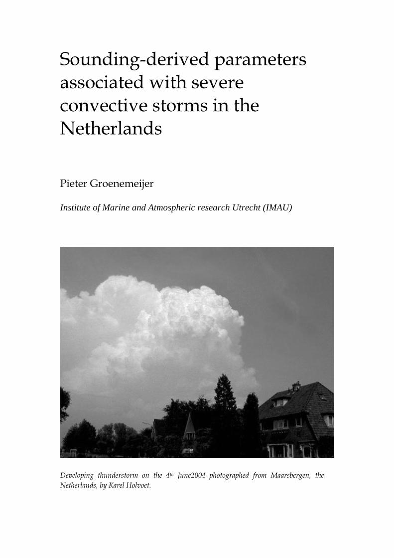
Sounding-derived parameters associated with severe convective storms in the Netherlands

Pieter Groenemeijer

Institute of Marine and Atmospheric research Utrecht (IMAU)

Developing thunderstorm on the 4th June2004 photographed from Maarsbergen, the Netherlands, by Karel Holvoet.

2

Abstract A study is presented focusing on the potential value of parameters derived from radiosonde data or data from numerical atmospheric models for the forecasting of severe weather associated with convective storms. In this study, parameters have been derived from proximity soundings to large hail, tornadoes (including waterspouts), severe convective wind events and thunderstorms in the Netherlands. 66365 radiosonde soundings from six stations in and around the Netherlands between 1 Dec 1976 to 31 Aug 2003 have been classified as being or not being associated with the severe weather types using observational data from voluntary observers, the Dutch National Meteorological Institute (KNMI) and lightning data from the U.K. Met. Office. Among the results were the following findings: Firstly, instability as measured by the Lifted Index or CAPE, the 0–1 km A.G.L. average mixing ratio and 0–6 km wind shear independently have considerable skill in distinguishing environments of large hail and of non-hail-producing thunderstorms. Secondly, for most severe wind gusts, the downward transport of high horizontal wind speeds to the surface, typically from an altitude of 2 km A.G.L., is the dominant process creating them, while a minority of events is primarily caused by strong downward vertical wind speeds developing in convective storms. Finally, for tornadoes, the major results are that the amount of CAPE released below 3 km A.G.L., is found to be high near waterspouts and weak tornadoes, while low-level shear is strong in environments of strong tornadoes and increases with increasing F-scale.

3

Contents

Abstract .................................................................................................... 2

Contents ................................................................................................... 3

1. Introduction ................................................................................... 5 1.1 The use of forecast parameters .............................................................. 5 1.2 This study.................................................................................................. 5

2. Theory of convective storms........................................................ 8 2.1 Ingredients for (severe) deep, moist convection ................................. 8 2.2 Latent instability and parcel theory ...................................................... 9

2.2.1 The choice of the parcel ......................................................................... 13 2.2.2 Limitations of parcel theory.................................................................. 15 2.2.3 Measures of instability ......................................................................... 16

2.3 Upward motion and convective initiation ......................................... 17 2.4 Wind shear and convective modes...................................................... 18

2.4.1 Single-cell storms ................................................................................. 18 2.4.2 Multicell line storms or squall-lines .................................................... 19 2.4.3 Supercells ............................................................................................. 20

2.5 Large hail ................................................................................................ 24 2.6 Wind gusts and downdrafts................................................................. 26

2.6.1 The pressure perturbation terms .......................................................... 26 2.6.2 Thermal buoyancy................................................................................ 27 2.6.3 Condensate loading .............................................................................. 28 2.6.4 Downdraft speed................................................................................... 28

2.7 Tornadoes ............................................................................................... 29 2.7.1 Mesocyclonic tornadoes (type 1) .......................................................... 30 2.7.2 Non-mesocyclonic tornadoes (type 2) .................................................. 31

3. Datasets and methodology ........................................................ 33 3.1 Severe convective weather events ....................................................... 33 3.2 Radiosonde data..................................................................................... 36 3.3 Lightning data ........................................................................................ 38 3.4 The definition of proximity .................................................................. 38 3.5 Categorization of the soundings.......................................................... 43

4

3.6 Climatological aspects of the severe weather events........................ 44 3.6.1 Large hail.............................................................................................. 45 3.6.2 Severe winds......................................................................................... 46 3.6.3 Tornadoes (and waterspouts) ............................................................... 47

4. Results and discussion................................................................ 49 4.1 Predictors for large hail......................................................................... 49

4.1.1 Instability ............................................................................................. 49 4.1.2 Deep-layer shear ................................................................................... 52 4.1.3 Low-level moisture and the wet-bulb zero level ................................... 54 4.1.4 Other parameters.................................................................................. 56

4.2 Predictors for severe winds .................................................................. 57 4.3 Predictors for tornadoes........................................................................ 61

4.3.1 Instability and Level of Free Convection.............................................. 62 4.3.2 Lifted Condensation Level .................................................................... 63 4.3.3 Wind shear ........................................................................................... 64

4.4 Average profiles for each severe weather type ................................. 68

5. Conclusions .................................................................................. 71 5.1 Summary of findings............................................................................. 71

5.1.1 Characterization of severe weather environments................................ 71 5.1.2 Implications of the results for forecasting ............................................ 73 5.1.3 Improving forecasting .......................................................................... 73

5.2 Suggestions for further research.......................................................... 74 5.2.1 Severe weather observations................................................................. 74 5.2.2 Climate change and the frequency of convective severe weather.......... 74 5.2.3 Use of better or more radiosonde data .................................................. 75

Acknowledgements.............................................................................. 76

References .............................................................................................. 77

Appendix A: Values of constants ....................................................... 82

Appendix B: Climatology of some parameters ................................ 82

Appendix C: Distribution diagrams of some parameters .............. 84

Appendix D: Tornado events in this study ...................................... 86

5

1. Introduction

1.1 The use of forecast parameters

Weather forecasters use various techniques to predict the occurrence of convective storms that produce thunder and lightning or thunderstorms. Hereby, parameters deduced from radiosonde data and numerical model data often play an important role. Examples of such parameters are the lifted index (Galway, 1956), the K-index (George, 1960) and the Boyden index (Boyden, 1963). These parameters are generally defined in terms of temperature and moisture variables at different altitudes in the troposphere and can be calculated using either observational data or forecast data from numerical atmospheric models.

The skill of various forecast parameters as predictors of thunderstorms in the Netherlands has recently been studied by Haklander (2002) and Haklander and van Delden (2003) (hereafter HVD). Their results have shown that the forecast skill varies greatly among the parameters when applied in the Netherlands.

Other forecast parameters that have been developed do not address the likelihood of thunderstorms, but merely the overall threat of severe weather associated with convective storms. Examples are the SWEAT index (Miller, 1972) and the index commonly referred to as the Craven Significant Severe index (Craven et al., 2002a). There are also parameters that address the threat of large hail, severe winds or tornadoes specifically. For example, the Energy-Helicity Index (EHI) (Davies and Johns, 1993) and the Significant Tornado Parameter (STP) (Thompson et al., 2002a, 2002b) were developed to be predictors of tornadoes. Forecast parameters for convectively-driven severe winds have been developed for example by Miller (1972) and McCann (1994) in the United States, and in the Netherlands by Ivens (1987).

1.2 This study

In this study, which is a follow-up of the HVD study, the following problem is addressed:

6

How can radiosonde-derived data be used to forecast some of the potentially hazardous phenomena that may accompany convective storms: severe wind gusts, large hail and tornadoes.

A slightly different approach is chosen compared with HVD as we have not tested the forecast skill of a large set of existing parameters. Instead a number of parameters has been selected that represents a single aspect of the atmospheric conditions. So, for example, instead of testing the quality of the Significant Tornado Parameter (Thompson et al., 2002), we have considered the various building blocks of this parameter, which in this case includes parameters like wind shear, instability and the lifted condensation level. It is thought that this approach will prevent to blur the view on the processes responsible for the severe weather phenomena. A number of studies using data from the United States have addressed approximately the same research question as that considered herein. These include the studies of Rasmussen and Blanchard (2002), Rasmussen (2003), Thompson et al. (2002a), Craven et al. (2002a), and Brooks and Craven (2002). In selecting the studied parameters, we have been influenced by those studies.

One may ask the question what the goal of the present study is, as it seems reasonable to assume that the results of the earlier studies have validity across the globe. Obviously, the laws of physics that determine the development of storms do not vary from place to place. The answer is that while parameters derived at a certain location may have some universal forecast skill, the same parameters are not necessarily everywhere the best discriminators between severe weather events and non-events. Typical weather conditions in the Netherlands, for example, make up only a small part of the data used in studies performed in the United States. To give an example, situations with high convective available potential energy (CAPE, see next section), are much more common in the United States. If results from the U.S. studies show a strong relation between some type of severe weather –tornadoes for example– and high values of CAPE, this may not be a useful result for forecasters in the Netherlands because high values of CAPE are only very rare in the Netherlands. The occasions on which the event occurs with low CAPE, that could be relatively rare in the United States, may be more typical of a Dutch tornado event. Other parameters than CAPE may then have a higher skill to discriminate between events and non-events in the Netherlands. It is most easily determined by using data from that area, which those parameters are.

We do however not imply that every single region of the globe needs its own detailed study, but merely that the forecast parameters have to be tested and –if necessary– calibrated for different climatological regions. In this study the

7

differences between the results obtained in the U.S. and in the Netherlands are discussed and an effort is made to try to explain them.

8

2. Theory of convective storms

2.1 Ingredients for (severe) deep, moist convection

The subject of this study is the occurrence of severe weather in association with convective storms that may or may not be accompanied by thunder. Convective storms are a manifestation of the overturning of the entire troposphere or a large part thereof, whereby condensation of water vapor occurs in updrafts. We will call this process deep, moist convection (DMC).

DMC can be regarded as an instability: a flow perturbation that initially grows by means of positive feedback on itself. It occurs only under the specific meteorological conditions that allow for its formation. DMC is often regarded as a process that converts convective available potential energy (CAPE) into kinetic energy. We will call the presence of CAPE latent instability1 following Normand (1938) and Galway (1956). Latent instability is not a real instability, but a situation that requires a forcing (that may need to be of a finite magnitude) to create a true instability: DMC.

The notion of latent instability and CAPE are based on the concept of a parcel of air that originates from some low atmospheric level and is lifted upward while it expands adiabatically. If it becomes less dense than its environment due to the release of latent heat, it will automatically accelerate upward, creating a real instability.

Above, we have identified two requirements for the occurrence of DMC:

• the presence of CAPE

• the presence of a forcing sufficiently large to release the CAPE.

1 Some use the term conditional instability to refer to situations having

CAPE. The term conditional instability is more frequently used to indicate the situation in which a layer of air has a lapse rates between wet-adiabatic and dry-adiabatic lapse rates.

9

In some cases however, very little or no CAPE is present near convective storms. Cases of squall lines occurring with no CAPE have for example been described in detail by Carbone et al. (1982, 1983) and Forbes (1985), occurring in California and the Netherlands respectively. The cases occurred in strong vertical wind shear and both produced a tornadoes. Dynamic instabilities may have played more important roles in these convective storms than the release of CAPE.

2.2 Latent instability and parcel theory

To find out if CAPE is present with a given vertical temperature and moisture profile, one should look if a parcel of air originating from some atmospheric level can acquire positive buoyancy when lifted by some process. The quantity buoyancy arises in the vertical momentum equation when it is written in terms of perturbations on a hydrostatically balanced base state. The vertical momentum equation in an ideal fluid can most elementarily be written as

g1dd

−∂∂

−=zp

tw

ρ. (1)

Herein, t is time, z is height, w is the vertical velocity, p is pressure, ρ is density and g the acceleration of gravity. We may decompose pressure and density in hydrostatically balanced components and deviations from hydrostatic equilibrium (denoted with primes), i.e. ρ = ρ0 + ρ' and p = p0 + p', where dp0/dz = – ρ0g. In case ρ' << ρ and p' << p, we can write:

g''1dd

ρρ

ρ−

∂∂

−=zp

tw

. (2)

The first term on the right-hand side is the pressure perturbation term and the second term is thermal buoyancy. The first term can be decomposed into dynamically induced pressure perturbations and buoyancy induced pressure perturbations p' = p'd + p'b, yielding

g''1'1

dd

ρρ

ρρ−

∂∂

−+∂

∂−=

zp

zp

tw bd . (3)

In this equation, the combination of underlined terms should be called buoyancy (B) according to Doswell and Markowski (2003). In the one-

10

dimensional context of parcel theory, pressure perturbations cannot be calculated. We therefore neglect dynamic pressure perturbations for now and consider buoyancy to be equal to thermal buoyancy (BT) as is traditionally done in parcel theory. In an ideal gas, at speeds much smaller than the speed of sound, a parcel's thermal buoyancy is dependent on its virtual temperature perturbation only (Emanuel, 1994). Virtual temperature is equal to temperature except for a small term that incorporates the effect of water vapor content on the density of the air. Virtual temperature, Tv, is given by

rrTTV +

+=

1ε1

, (4)

where r is the mixing ratio of water vapor air, and ε is the constant Rd/Rv = 0.6220. Rd is the gas constant for dry air and Rv the gas constant of water vapor. The thermal buoyancy BT of a parcel is given by

g'

v

vT T

TB = , (5)

where Tv' is the virtual temperature difference between the parcel and its environment, vT is the average virtual temperature (we assume Tv' << vT . Note that we assume here that a parcel contains only air and water vapor, but no liquid or solid water (see section 2.2.2).

We make the assumption here that no exchange of heat or mass takes place between a lifted parcel and its environment. In case no condensation of water vapor takes place during the ascent of a parcel, its potential temperature θ is conserved, which is defined as

pd

d

cR

0⎟⎟⎠

⎞⎜⎜⎝

⎛=

pp

Tθ , (6)

where p0 is some standard pressure level, usually chosen to be 1000 hPa, and cpd is the heat capacity of dry air at constant pressure. If water vapor condenses to liquid water during ascent, its equivalent potential temperature θe is conserved. It is often assumed that at least part of the condensed water falls out of the parcel, so that we cannot speak of adiabatic ascent, since it implies that an exchange of mass and heat takes place. If we assume that all water falls out of the parcel, we have a process called pseudo-adiabatic ascent. During pseudo-adiabatic ascent

11

the so-called pseudo-equivalent potential temperature θep of the parcel is conserved. The difference between θep and θe is usually small. An analytical expression for θep cannot be given, but an accurate approximation has been developed by Bolton (1980):

( )

( ) ⎟⎟⎠

⎞⎜⎜⎝

⎛⎟⎠⎞

⎜⎝⎛ −+⎟⎟

⎠

⎞⎜⎜⎝

⎛=

−

54.233760.811exphPa1000*

28.012854.0

Trr

pT

r

epθ (7)

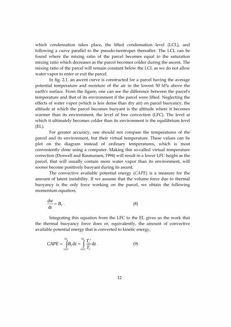
Fig. 2.1. Skew-T log p thermodynamic diagram, on which temperature and dew point temperature data from a radiosonde ascent are plotted. The diagram shows isobars, isotherms, lines of equal potential temperature θ (isentropes), lines of equal pseudo-equivalent potential temperature θep (pseudo-isentropes), lines of equal mixing ration r (isohumes). An ascent curve T(p) of a parcel having the averaged temperature and mixing ratio of the lowest 50 hPa has been constructed.

Using a thermodynamic diagram that shows lines of equal θ (isentropes), θep (pseudo-isentropes) and of equal saturation mixing ratio rs, it is relatively straightforward to draw the curve T(p) that a parcel would follow during ascent. Fig. 2.1 is a so-called skew-T, log-p thermodynamic diagram. Starting from the position of the parcel in the diagram, the T(p)-curve of the parcel can be constructed by following a curve parallel to the isentropes up to the level at

12

which condensation takes place, the lifted condensation level (LCL), and following a curve parallel to the pseudo-isentropes thereafter. The LCL can be found where the mixing ratio of the parcel becomes equal to the saturation mixing ratio which decreases as the parcel becomes colder during the ascent. The mixing ratio of the parcel will remain constant below the LCL as we do not allow water vapor to enter or exit the parcel.

In fig. 2.1. an ascent curve is constructed for a parcel having the average potential temperature and moisture of the air in the lowest 50 hPa above the earth's surface. From the figure, one can see the difference between the parcel's temperature and that of its environment if the parcel were lifted. Neglecting the effects of water vapor (which is less dense than dry air) on parcel buoyancy, the altitude at which the parcel becomes buoyant is the altitude where it becomes warmer than its environment, the level of free convection (LFC). The level at which it ultimately becomes colder than its environment is the equilibrium level (EL).

For greater accuracy, one should not compare the temperatures of the parcel and its environment, but their virtual temperature. These values can be plot on the diagram instead of ordinary temperatures, which is most conveniently done using a computer. Making this so-called virtual temperature correction (Doswell and Rasmussen, 1994) will result in a lower LFC height as the parcel, that will usually contain more water vapor than its environment, will sooner become positively buoyant during its ascent.

The convective available potential energy (CAPE) is a measure for the amount of latent instability. If we assume that the volume force due to thermal buoyancy is the only force working on the parcel, we obtain the following momentum equation,

TBtw

=dd

. (8)

Integrating this equation from the LFC to the EL gives us the work that the thermal buoyancy force does or, equivalently, the amount of convective available potential energy that is converted to kinetic energy,

∫∫ ==EL

LFC

EL

LFC

d'd zTTzBCAPE

v

vT . (9)

13

When virtual temperature is approximated by temperature, the amount of CAPE is proportional to the area between the parcel ascent curve and the environmental temperature curve in a skew-T, log-p diagram like fig. 2.1.

CAPE is released when a parcel exceeds its LFC. For this to occur the rising parcel often has to overcome an amount of negative energy. This energy is called convective inhibition (CIN) and is represented by the area between the parcel's and the environmental temperature curves just below the LFC.

∫∫ ==EL

level source

LFC

level source

d'd zTTzBCIN

v

vT (10)

For air parcels to be able to reach their LFC, CIN has to be reduced to low values, so that it can be overcome by upward momentum the parcel may initially have.

2.2.1 The choice of the parcel When assessing what amount of CAPE can theoretically be released in convective storms, an important issue is to find the most appropriate parcel to lift. It is preferred that the parcel is representative of the air that enters convective updraft. In typical storms that form after a day of abundant sunshine, one can expect that the air flowing into a storm's updraft originates from a layer of air just above the earth's surface, as this is commonly the air that can become most buoyant when lifted (i.e. having the highest equivalent potential temperature, θep). An important question is what the thickness of the source layer is. The answer to this question determines which θep should be chosen to be the θep of the theoretical lifted parcel.

It is important to realize that many convective storm situations are characterized by a strong decrease with height of temperature and moisture content just above the earth's surface, indicative of turbulent transport of heat and moisture. As a consequence θep values decrease rapidly with height as well. This means that CAPE becomes very sensitive to the depth of the mixed layer that the parcel represents.

Craven et al. (2002b) have calculated LCL heights using temperature and moisture values at standard 2 meters above the surface and the LCL heights calculated using a mixing ratio and potential temperature averaged over the lowest 100 hectopascals for a large number of soundings. These were verified with cloud base heights observed by ceilometers, that should correspond with the LCL heights. Their results show that over the Central Plains of the United States,

14

the median surface-based CAPE was more than twice the median of the 100 hPa mixed-layer CAPE and that surface based parcels often had too low LCL heights, while the mixed-layer parcel LCL heights were generally in reasonable agreement with the ceilometer observations. This suggests that the air flowing into convective updrafts is more likely to be a mixture of air at various heights in the boundary layer than to originate from 2 m altitude above the earth's surface. Thereby it seems that it is better to use the mixed layer for CAPE calculations.

In some circumstances, DMC is not sustained from a layer above the earth's surface, but from a layer at a higher altitude. This often occurs at night when a radiative inversion is present just above the surface, or, for example, on the cold side of a surface warm front. In such cases of elevated convection one may wish to consider instead the parcel that has the highest θep and thereby the highest CAPE. The CAPE value calculated using this parcel's properties is called the most-unstable CAPE (m.u.-CAPE). In this study, the most-unstable parcel has been defined as the parcel having the highest θep within the layer between the surface and 3000 m A.G.L. We will use the prefix m.u.- for all variables calculated with the most-unstable parcel and the prefix 50-m.l.- for all variables calculated using the 50 hPa A.G.L. mean-layer parcel.

50-m.l.-CAPE / m.u.-CAPE values exceeded... ( J/kg )

once per week

once per month

once per season

once in the dataset (maximum)

DJF 11 / 153 59 / 328 122 / 413 548 / 730

MAM 42 / 343 183 / 905 520 / 1661 2466 / 2992

JJA 154 / 747 612 / 1631 1145 / 2285 3309 / 4535

SON 53 / 342 184 / 824 348 / 1198 1239 / 2360

Table 1. Typical return periods of 50-m.l.-CAPE and m.u.-CAPE values.

From some climatological values derived from the De Bilt soundings between 1 January 1976 and 31 December 2002 at 12 UTC, we can see that their magnitudes differ quite strongly. The highest values of 50-m.l.-CAPE and m.u.-CAPE that have been measured during the entire period are 3309 and 4535 J/kg respectively, differing approximately a factor 1.4. Looking at wintry and more common, lower values the relative difference between the two variants of CAPE becomes even bigger. For example, in winter the value corresponding with a return period of one month is 59 J/kg for 50-m.l.-CAPE and 328 J/kg for m.u.-CAPE, i.e. differing almost by a factor 6. It should therefore be stressed that the two should never be confused.

15

2.2.2 Limitations of parcel theory The severity of convective storms is to some extent related to the vertical speed within its updraft(s). For a storm to produce large hail stones, a prerequisite is a strong upward airflow that can keep large hail stones aloft while they grow to a considerable size. Obviously, in tornadoes strong upward velocities play an important role as well.

It is however not trivial to estimate a storm's updraft speed. A very simple estimate can be obtained by assuming all CAPE available to a parcel that enters the updraft is converted to kinetic energy. In this case. the maximum upward speed would be reached at the equilibrium level where all CAPE has been released. The maximum upward speed would then be

CAPEw 2EL = (11)

Unfortunately this estimate is not likely to be very accurate as a number of fundamental imperfections to parcel theory have been ignored. Firstly, we have assumed that entrainment of environmental air into the parcel does not occur. This is quite unrealistic as it can be shown using similarity theory that entrainment of environmental air occurs in both thermals and thermal plumes (see Emanuel, 1994, chapter 2). The effects of entrainment include a transport of less upward vertical momentum into the parcel and a reduction of the parcel's buoyancy. Secondly, we have neglected pressure perturbations.

Dynamic pressure perturbations p'd can seriously affect the flow. In an isolated updraft in a non-sheared environment the dynamic pressure gradient will counteract the upward buoyancy force working on a parcel. In a sheared flow it can also be directed upward and add to the updrafts' strength. Pressure perturbations related to buoyancy p'b have been neglected as well. Thirdly, in parcel theory the effects of liquid and solid water on buoyancy have been neglected. The buoyancy of a parcel can become significantly smaller as a result of water loading or even negative with respect to the unperturbed environment. In fact, it is thought that water loading is a major factor in the creation of convective downdrafts (e.g. Byers and Braham, 1954). Finally, any radiational exchange of heat is ignored in parcel theory.

All this is reason not to use the magnitude of latent instability only to assess the maximum updraft speed in a storm. Though a velocity can certainly be calculated from a CAPE value by the relationship CAPEw 2EL = , it generally is not an accurate way to predict vertical motion in storms (Doswell and Rasmussen, 1994).

16

2.2.3 Measures of instability In this study a few other measures of instability besides CAPE have been used for several reasons. Firstly, the Lifted Index LI (Galway, 1956) is defined as the parcel's (virtual) temperature excess at the 500 hPa level:

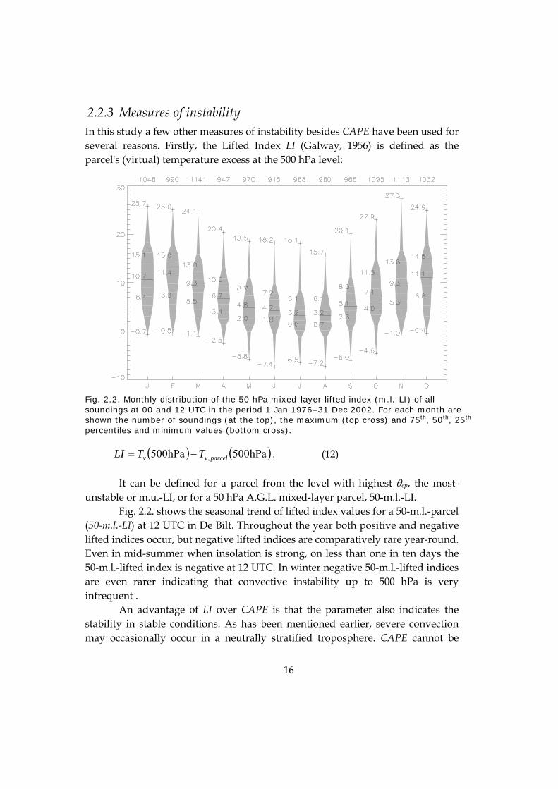
Fig. 2.2. Monthly distribution of the 50 hPa mixed-layer lifted index (m.l.-LI) of all soundings at 00 and 12 UTC in the period 1 Jan 1976–31 Dec 2002. For each month are shown the number of soundings (at the top), the maximum (top cross) and 75th, 50th, 25th percentiles and minimum values (bottom cross).

( ) ( )hPa500hPa500 , parcelvv TTLI −= . (12)

It can be defined for a parcel from the level with highest θep, the most-unstable or m.u.-LI, or for a 50 hPa A.G.L. mixed-layer parcel, 50-m.l.-LI.

Fig. 2.2. shows the seasonal trend of lifted index values for a 50-m.l.-parcel (50-m.l.-LI) at 12 UTC in De Bilt. Throughout the year both positive and negative lifted indices occur, but negative lifted indices are comparatively rare year-round. Even in mid-summer when insolation is strong, on less than one in ten days the 50-m.l.-lifted index is negative at 12 UTC. In winter negative 50-m.l.-lifted indices are even rarer indicating that convective instability up to 500 hPa is very infrequent .

An advantage of LI over CAPE is that the parameter also indicates the stability in stable conditions. As has been mentioned earlier, severe convection may occasionally occur in a neutrally stratified troposphere. CAPE cannot be

17

used to distinguish between neutral and very stable conditions, while the LI can do that, which is convenient in statistical calculations.

A drawback of the LI is that conditions at exactly 500 hPa may for some reason not be representative of the rest of the mid-troposphere. This may be the case when, for example, a shallow relatively warm layer is present at that level. Additionally, in some cases when the Lifted Index is positive indicating negative parcel buoyancy at 500 hPa, latent instability may be present below this level which may give an incorrect assessment of instability.

A measure of the amount of instability present nearby the earth's surface is the amount of CAPE that is released below 3 km A.G.L. (Rasmussen, 2003), which will herein be referred to as CAPE3km. This parameter has been considered in this study as well and can be calculated both for a mixed-layer parcel and the most-unstable parcel.

∫∫ ==AGL km 3

LFC

AGL km 3

LFC

d'

d3 zTT

zBkmCAPEv

vT (13)

2.3 Upward motion and convective initiation

As was argued before, convective storms form in areas where not only CAPE is present, but also a forcing that is sufficiently large to release the CAPE. According to parcel theory, the forcing should help the parcel to overcome convective inhibition (CIN). A broad range of processes on the synoptic scale to the scale of the convection itself can play a role in initiating convection. Convective initiation is often accomplished through rising motions.

Both rising motions on the scale of hundreds of kilometers of as well as on the scale of thermals can be interpreted in the context of parcel theory. Large- or mesoscale rising motions can cool the warm layer that inhibits the deep convection by adiabatic ascent until CIN has disappeared and convective storms can initiate. Rising motions in the boundary layer on the scale of thermals contain the kinetic energy for an air parcel (i.e. the thermal) needed to overcome the convective inhibition, while the reference state remains unchanged.

Reality is more complicated as parcels and reference states are only simplifications of reality. Convective initiation is often associated with rising motions on various scales and may for example be related to frontal circulations, thermals, orographic lifting, convergence lines or horizontal convective rolls. Single-site radiosonde observations that form the basis of this study however, do

18

not reveal the presence of rising motion, so that initiation was not an issue in this study. Another follow-up study of HVD by van Zomeren (2005) and van Zomeren and van Delden (2005) addresses this subject.

2.4 Wind shear and convective modes

Wind shear or vertical wind shear is the derivative of the wind field with height. It is often expressed as the magnitude of the vector difference between the horizontal winds at two specified altitudes, or bulk shear.

Fig. 2.3. Life cycle of a single cell storm. The contours denote radar reflectivity (* 10 dBz). The bottom figure shows the reflectivity of a pulse storm. Adapted from Chisholm and Renick (1972).

We will do so in this study, although strictly speaking it is incorrect. Wind shear has an important influence on deep convection as it can cause separation of up- and downdrafts, which usually increases the longevity of convective storms and causes dynamic pressure perturbations that have a strong influence on their organization.

2.4.1 Single-cell storms When low shear is present, single cells or ordinary cells can be expected to form, storms that have relatively short lifetimes. Fig. 2.3. shows the life cycle of an ordinary cell. In its initial stage a convective bubble forms as a quantity of air has

19

reached its LFC. This subsequently rises upward until it reaches the level where its buoyancy vanishes. Neglecting water loading, entrainment, pressure perturbations and radiational heat exchange, this level corresponds to the equilibrium level (EL) predicted by parcel theory.

Gradually, precipitation forms within the cloud, which negatively impacts the air's buoyancy. When the precipitation falls down, its evaporation cools the unsaturated sub-cloud layer, which further reduces buoyancy. A mass of cold air, frequently referred to as a cold pool, forms beneath the convective updraft as a result. As it spreads out over the earth’s surface, it cuts off the inflow of warm air flowing into the updraft. The remaining precipitation falls out and smaller water droplets and ice particles evaporate. This life cycle takes typically 30 to 50 minutes. Single cells rarely produce severe weather. When they do, it is often in environments of extreme latent instability. These storms have very high tops and are sometimes called pulse storms. Single cells are often the building blocks of larger convective systems.

2.4.2 Multicell line storms or squall-lines When shear is larger, multicell storms are likely to form. These are storms consisting of multiple convective updrafts and downdrafts. The key to the genesis of a multicell storm is the development of new convective cells along the boundary of the cold pool originating from an older cell. Such a boundary is often called an outflow boundary or gust front. The initiation of new cells is most likely to happen on the downshear side of the convective complex (i.e. the direction from which the low-level wind blows in a storm-relative reference frame) and is caused by rising motions that result from interaction of the cold pool boundary and the environmental –latently unstable– air. During the ascent of this air, new air parcels reach their level of free convection and develop into new convective cells. As a result, multicell complexes are clusters of convective cells in various stages of their life cycles.

Compared to single cell storms, multicell clusters have a higher probability of producing severe weather including damaging winds, large hail and occasionally weak tornadoes.

A distinction can be made between multicell clusters and multicell lines, the latter also being referred to as squall lines. Squall lines form when convection is triggered by upward motions along some type of boundary, for example a cold front or a convergence line so that the deep convection that ensues will also be linearly organized. Storms can also become linearly organized due to the merging

20

of their outflows and the resulting formation of one single outflow boundary along which new convective cells are triggered.

In environments of high wind shear, the leading edge of squall-lines may exhibit vortices caused by the tilting of environmental horizontal vorticity (Weisman and Davis, 1998), similar to the tilting mechanism at work in supercells (see next paragraph). These should not be confused with the larger vortices that may form on their extreme ends (book-end vortices). If the along-line vortices are strong, one may speak of embedded supercells (see next section), that may produce tornadoes (e.g. Carbone, 1983).

2.4.3 Supercells When vertical wind shear is large, supercell storms may form. Supercells have a longer lifetime than multicells and single cells. A supercell is a thunderstorm having a deep and persistent rotating updraft (Burgess and Doswell, 1993). Supercells are known for their capability to produce various types of severe weather. An important reason for this is that supercells may contain very high vertical velocities within both updrafts and downdrafts that may significantly exceed the vertical velocities predicted by parcel theory. Weisman and Klemp (1984) have shown that in supercells effects of dynamically induced vertical pressure gradients on the vertical speed in the updraft may be as important as the effects of buoyancy. These vertical pressure gradients form as a result of the interaction of the updraft within a strongly sheared flow.

In a study using proximity soundings, Doswell and Evans (2003) found that the median value of surface to 6 km A.G.L. shear near supercells was slightly above 20 m/s.

21

Fig. 2.4. As in fig 2. except for the magnitude of the wind vector difference between 10m and 6 km A.G.L. in m/s of all soundings at 12 UTC in the period 1 Jan 1976 – 31 Dec 2002.

From fig. 2.4. it can be seen that 0–6 km wind shear values of around 20 ms–1 or more are considerably above the climatological median values in summer in De Bilt, when high CAPE values that can sustain strong convection are most likely. In winter strong shear is more common, but high CAPE values are rare.

dvdz

v-c

vortex lines

peak

storm-relativemean flow

Fig. 2.5. The creation of vertical vorticity in an updraft in a sheared flow (see text for explanation). v is the low-level wind vector, c the storm motion vector, ω the vorticity vector. Based on a figure from Davies-Jones (1984).

Davies-Jones (1984) has provided a physical model to understand how a rotating updraft, also known as a mesocyclone, can develop. He has shown that

22

upward vertical motion is correlated with positive vertical vorticity in certain vertical wind profiles. In a mathematical derivation he establishes an expression for their correlation coefficient.

The theory can be interpreted as follows. An isentropic or pseudo-isentropic surface (depending on whether we consider unsaturated or saturated air) is considered near a convective updraft (see fig. 2.5). Because (equivalent) potential temperature is a conserved scalar2, vertical motions deform this surface. This is consistent with the observation that since the isentropic surfaces are material surfaces, the flow must follow them. This also implies that a initiating convective updraft is associated with an upward deformation of the surface. Another consequence is that any storm-relative horizontal flow in this surface will be upward on the upwind side of the displacement peak and downward on its downwind side.

Whenever there is vertical wind shear, there will be vortex lines that are horizontally oriented initially. Because (equivalent)potential vorticity, θ∇⋅ω (where vorticity vω ×∇≡ ) is conserved, it can be inferred that a vortex line that lies in an isentropic surface initially (i.e. zero potential vorticity) must remain within that surface. The vortex lines may have a component parallel to the storm relative wind as in fig. 2.5 which is called streamwise vorticity. If this is the case, the vortex lines must be tilted into the vertical near the displacement peak. This results in vertical vorticity (positive and negative) at the up- and downwind sides of the displacement peak viewed in a reference frame moving with the storm at speedc . It is important to note that the largest vertical motions are not associated with the location of the largest displacement of the surface if horizontal storm-relative winds are present, but upstream of the peak. This implies there is a positive correlation of upward vertical motion and cyclonic vorticity.

Vorticity in the environment of the storm that is streamwise with respect to the storm's inflow in this example of a storm moving at horizontal speed c can be written as

ωcvcvω ⋅

−−

=streamwise . (14)

2 By good approximation in the case of equivalent potential temperature.

23

Multiplying this with the speed at which the flow enters the updraft region, cv − , gives the rate at which streamwise vorticity flows enters the updraft

region. This quantity is storm relative helicity (SRH*),

ωcv ⋅−= )(*SRH , (15)

which is usually integrated over the entire layer that constitutes the inflow to the storm, often from the earth's surface to 1, 2 or 3 kilometers A.G.L.. From here on we will only refer to the integrated version of storm-relative helicity (SRH). This gives

( ) zSRH d ωcv ⋅−= ∫ . (16)

which, neglecting vertical velocity components away from the storm, equals

( )∫ −×∂

∂= z

zSRH h

h dcvv

. (17)

SRH integrated from the earth's surface to 3 km A.G.L. has been found to be high in supercell environments (Rasmussen and Blanchard, 1992). SRH integrated up to 1 km A.G.L. is a relatively good discriminator between tornadic and nontornadic supercells (Rasmussen, 2003).

The value of SRH depends strongly on the storm motion vector c. For supercell storms, this motion is to the right of the lower tropospheric mean wind vector. When calculating SRH without knowing the motion vectors of storms in that environment, the storm-motion must be estimated. We have here made the empirical assumption that the storm motion was equal to that which is given by the Internal Dynamics (ID) method (Bunkers et al., 2000):

( )⎟⎟⎠

⎞⎜⎜⎝

⎛

−×−

⋅+=

∫

∫m 10km 6

m 10km 6km 6

m 10

km 6

m 10 k̂

d

d

vvvv

vc D

z

zh

(18)

where v6 km and v6 km are the horizontal winds at 6 km and 10 m A.G.L. respectively, D is a constant of 7.5 m/s and k̂ is the upward unit vector. This formula has been demonstrated to work well for supercells that move right of the

24

main wind, which are the most frequent. For more information about the this formula, please refer to Bunkers et al (2000).

2.5 Large hail

Fig. 2.6. Large hailstone that fell in Elburg, the Netherlands, on the 6th of June, 1998. Photograph by John Kambeel.

Important for the formation of hailstones is the fact that within convective updrafts, water vapor condenses to cloud droplets (Knight and Knight, 2001). As they are advected above the level at which the wet-bulb temperature drops below zero, they will get a temperature below 0 ºC or supercooled. Cloud droplets can become as cool as -40 ºC before they freeze.

Hailstone growth occurs within storm updrafts as a piece of ice, the forming hailstone, whose fall velocity with respect to air is approximately compensated by the updraft velocity, collides with lighter supercooled liquid water droplets that are carried upward. Upon collision the droplets freeze and add to the size of the hailstone.

An important issue that has been addressed by many researchers, is how the initial ice particle –the hail-embryo that is typically a few millimeters in diameter– may end up in the storm's updraft. It cannot be formed within the same region in the updraft as processes to form millimeter-sized particles take about 20 to 30 minutes. This would imply that these small particles would have left the updraft, that is strong enough to sustain the larger hailstones, before further growth can begin. Many ways how hail-embryo's can enter a strong updraft have been discovered including

• ingestion of embryos from nearby storms or large cumulus clouds,

25

• the freezing of drops that originate from other hailstones having a water coating,

• the formation of embryos in an early (weak) stage of the updraft and others (see Knight and Knight (2001) for more information).

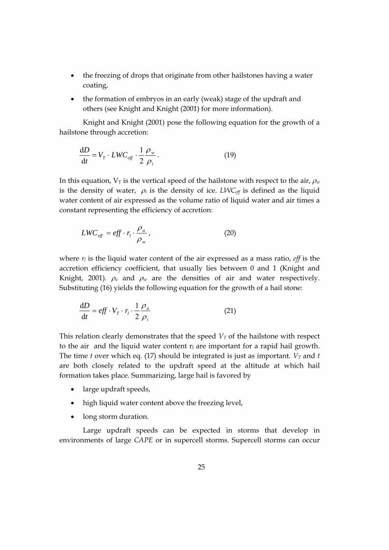
Knight and Knight (2001) pose the following equation for the growth of a hailstone through accretion:

i

weffT LWCV

tD

ρρ

21

dd

⋅⋅= . (19)

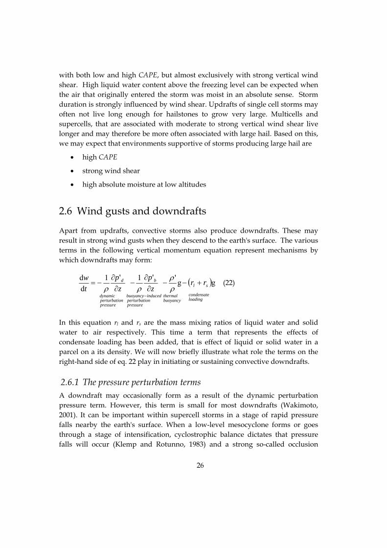
In this equation, VT is the vertical speed of the hailstone with respect to the air, ρw is the density of water, ρi is the density of ice. LWCeff is defined as the liquid water content of air expressed as the volume ratio of liquid water and air times a constant representing the efficiency of accretion:

w

aleff reffLWC

ρρ

⋅⋅= , (20)

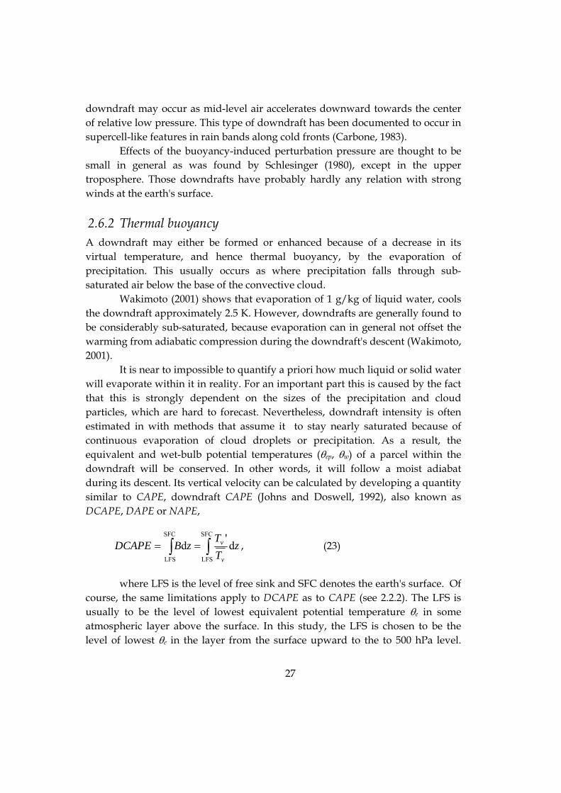
where rl is the liquid water content of the air expressed as a mass ratio, eff is the accretion efficiency coefficient, that usually lies between 0 and 1 (Knight and Knight, 2001). ρa and ρw are the densities of air and water respectively. Substituting (16) yields the following equation for the growth of a hail stone:

i

alT rVeff

tD

ρρ

21

dd

⋅⋅⋅= (21)

This relation clearly demonstrates that the speed VT of the hailstone with respect to the air and the liquid water content rl are important for a rapid hail growth. The time t over which eq. (17) should be integrated is just as important. VT and t are both closely related to the updraft speed at the altitude at which hail formation takes place. Summarizing, large hail is favored by

• large updraft speeds,

• high liquid water content above the freezing level,

• long storm duration.

Large updraft speeds can be expected in storms that develop in environments of large CAPE or in supercell storms. Supercell storms can occur

26

with both low and high CAPE, but almost exclusively with strong vertical wind shear. High liquid water content above the freezing level can be expected when the air that originally entered the storm was moist in an absolute sense. Storm duration is strongly influenced by wind shear. Updrafts of single cell storms may often not live long enough for hailstones to grow very large. Multicells and supercells, that are associated with moderate to strong vertical wind shear live longer and may therefore be more often associated with large hail. Based on this, we may expect that environments supportive of storms producing large hail are

• high CAPE

• strong wind shear

• high absolute moisture at low altitudes

2.6 Wind gusts and downdrafts

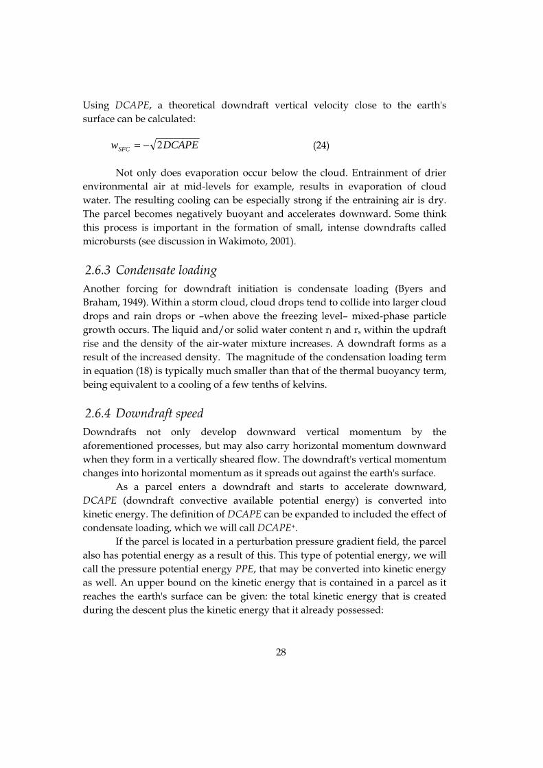
Apart from updrafts, convective storms also produce downdrafts. These may result in strong wind gusts when they descend to the earth's surface. The various terms in the following vertical momentum equation represent mechanisms by which downdrafts may form:

( )loadingcondensate

sl

buoyancythermal

pressureonperturbatiinducedbuoyancy

b

pressureonperturbati

dynamic

d rrz

pz

ptw gg'

'1'1dd

+−−∂

∂−

∂∂

−=

−ρρ

ρρ (22)

In this equation rl and rs are the mass mixing ratios of liquid water and solid water to air respectively. This time a term that represents the effects of condensate loading has been added, that is effect of liquid or solid water in a parcel on a its density. We will now briefly illustrate what role the terms on the right-hand side of eq. 22 play in initiating or sustaining convective downdrafts.

2.6.1 The pressure perturbation terms A downdraft may occasionally form as a result of the dynamic perturbation pressure term. However, this term is small for most downdrafts (Wakimoto, 2001). It can be important within supercell storms in a stage of rapid pressure falls nearby the earth's surface. When a low-level mesocyclone forms or goes through a stage of intensification, cyclostrophic balance dictates that pressure falls will occur (Klemp and Rotunno, 1983) and a strong so-called occlusion

27

downdraft may occur as mid-level air accelerates downward towards the center of relative low pressure. This type of downdraft has been documented to occur in supercell-like features in rain bands along cold fronts (Carbone, 1983).

Effects of the buoyancy-induced perturbation pressure are thought to be small in general as was found by Schlesinger (1980), except in the upper troposphere. Those downdrafts have probably hardly any relation with strong winds at the earth's surface.

2.6.2 Thermal buoyancy A downdraft may either be formed or enhanced because of a decrease in its virtual temperature, and hence thermal buoyancy, by the evaporation of precipitation. This usually occurs as where precipitation falls through sub-saturated air below the base of the convective cloud.

Wakimoto (2001) shows that evaporation of 1 g/kg of liquid water, cools the downdraft approximately 2.5 K. However, downdrafts are generally found to be considerably sub-saturated, because evaporation can in general not offset the warming from adiabatic compression during the downdraft's descent (Wakimoto, 2001).

It is near to impossible to quantify a priori how much liquid or solid water will evaporate within it in reality. For an important part this is caused by the fact that this is strongly dependent on the sizes of the precipitation and cloud particles, which are hard to forecast. Nevertheless, downdraft intensity is often estimated in with methods that assume it to stay nearly saturated because of continuous evaporation of cloud droplets or precipitation. As a result, the equivalent and wet-bulb potential temperatures (θep, θw) of a parcel within the downdraft will be conserved. In other words, it will follow a moist adiabat during its descent. Its vertical velocity can be calculated by developing a quantity similar to CAPE, downdraft CAPE (Johns and Doswell, 1992), also known as DCAPE, DAPE or NAPE,

∫∫ ==SFC

LFS

SFC

LFS

d'

d zTT

zBDCAPEv

v , (23)

where LFS is the level of free sink and SFC denotes the earth's surface. Of course, the same limitations apply to DCAPE as to CAPE (see 2.2.2). The LFS is usually to be the level of lowest equivalent potential temperature θe in some atmospheric layer above the surface. In this study, the LFS is chosen to be the level of lowest θe in the layer from the surface upward to the to 500 hPa level.

28

Using DCAPE, a theoretical downdraft vertical velocity close to the earth's surface can be calculated:

DCAPEwSFC 2−= (24)

Not only does evaporation occur below the cloud. Entrainment of drier environmental air at mid-levels for example, results in evaporation of cloud water. The resulting cooling can be especially strong if the entraining air is dry. The parcel becomes negatively buoyant and accelerates downward. Some think this process is important in the formation of small, intense downdrafts called microbursts (see discussion in Wakimoto, 2001).

2.6.3 Condensate loading Another forcing for downdraft initiation is condensate loading (Byers and Braham, 1949). Within a storm cloud, cloud drops tend to collide into larger cloud drops and rain drops or –when above the freezing level– mixed-phase particle growth occurs. The liquid and/or solid water content rl and rs within the updraft rise and the density of the air-water mixture increases. A downdraft forms as a result of the increased density. The magnitude of the condensation loading term in equation (18) is typically much smaller than that of the thermal buoyancy term, being equivalent to a cooling of a few tenths of kelvins.

2.6.4 Downdraft speed Downdrafts not only develop downward vertical momentum by the aforementioned processes, but may also carry horizontal momentum downward when they form in a vertically sheared flow. The downdraft's vertical momentum changes into horizontal momentum as it spreads out against the earth's surface.

As a parcel enters a downdraft and starts to accelerate downward, DCAPE (downdraft convective available potential energy) is converted into kinetic energy. The definition of DCAPE can be expanded to included the effect of condensate loading, which we will call DCAPE+.

If the parcel is located in a perturbation pressure gradient field, the parcel also has potential energy as a result of this. This type of potential energy, we will call the pressure potential energy PPE, that may be converted into kinetic energy as well. An upper bound on the kinetic energy that is contained in a parcel as it reaches the earth's surface can be given: the total kinetic energy that is created during the descent plus the kinetic energy that it already possessed:

29

horkinsfckin EPPEDCAPEE ,, ++≤ + (25)

Likely, dissipation will lead to lower kinetic energy in reality. According to the model described here, strong wind gusts can be expected when

• horizontal wind speed at the altitude where the downdraft originates is strong, to allow for the transport of horizontal momentum;

• DCAPE is high, as this enhances the downdraft's downward velocity;

• and to a lesser extent when...

• conditions are favorable for mesocyclonic storms (i.e. supercells), as they may allow for occlusion downdrafts;

• the mixing ratio of the air entering the updraft is large, so that liquid water content in updrafts may become large, allowing for downburst intensification because of high water loading.

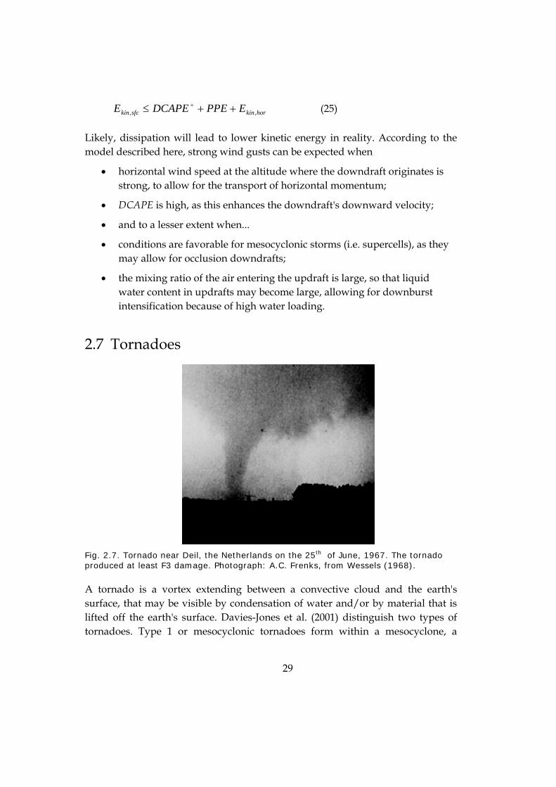
2.7 Tornadoes

Fig. 2.7. Tornado near Deil, the Netherlands on the 25th of June, 1967. The tornado produced at least F3 damage. Photograph: A.C. Frenks, from Wessels (1968).

A tornado is a vortex extending between a convective cloud and the earth's surface, that may be visible by condensation of water and/or by material that is lifted off the earth's surface. Davies-Jones et al. (2001) distinguish two types of tornadoes. Type 1 or mesocyclonic tornadoes form within a mesocyclone, a

30

larger-scale parent circulation. Type 2 or non-mesocyclonic tornadoes are not associated with a mesocyclonic circulation. They are thought to form often by the rolling-up of a vortex sheet along a wind-shift line into individual vortices. Type 2 tornadoes are generally weak.

2.7.1 Mesocyclonic tornadoes (type 1) Mesocyclonic tornadoes occur both with isolated supercell storms and supercells embedded within larger convective systems. Although the formation of mesocyclonic tornadoes is not completely understood, it has been observed with Doppler radar that they form under mesocyclones that are strong at low altitudes above the surface, although this is not a guarantee that a tornado will form (e.g. Trapp, 1999). Nevertheless, an important question is how a strong low-level mesocyclone can form. Rotunno and Klemp (1985) have identified two sources for updraft rotation:

• tilting of streamwise horizontal vorticity originating from the storm's environment

• tilting of streamwise horizontal vorticity created by the storm itself by baroclinic processes

They found that rotation at mid-levels is primarily associated with the tilting of environmental vorticity, while low-level rotation is caused by tilting of the streamwise horizontal vorticity created by the storm itself.

Recent studies have indicated that tornadic environments are often characterized by strong wind shear in the 0–1 km layer, which implies the presence of large horizontal vorticity (Brooks and Craven, 2002; Craven et al 2002a; Monteverdi et al., 2001). Other evidence of this includes the study by Rasmussen (2003) showing that storm-relative helicity (SRH, eq. 16, 17) integrated up to 1 km A.G.L. -observed with radiosondes in the environment of the storm- is a good discriminated rather well between tornadic and non-tornadic supercells. This suggests that the tilting of environmental horizontal vorticity may be important for the formation of tornadoes, despite Rotunno and Klemp's study that suggested the generation of vorticity within the storm itself to lead to low-level rotation. It is possible, too, that the low-level shear is important for tornadogenesis because of another reason than simply the tilting of the associated vorticity.

A strong association has been found between tornadoes and low LFC heights (Davies, 2004). Low LFC heights imply that rising air gets a positive thermal buoyancy at a low height above the earth's surface. Upward acceleration

31

may be expected to start at low altitudes as well. This implies that strong vortex stretching can be expected near the surface, so that there is a strong amplification of vertical vorticity and a positive effect on tornadogenesis.

Researchers have also found that strong tornadoes are generally associated with low lifted condensation levels (Brooks and Craven, 2002; Craven et al 2002a; Rasmussen and Blanchard, 1992). The interpretation of this result is less straightforward. Davies (2004) argues that there is a relation between the height of the LCL and the height of the LFC: when LFC heights are low, LCL heights must be low as well since the LCL is located below the LFC. The opposite, however, is not true: a low LCL height does not imply the LFC height is low as well. Nevertheless, part of the relation between low LCL heights and tornado occurrence may be the same as that for low LFC heights.

Another theory that explains why LCL height could be of importance for tornado formation is the following. Air parcels that enter a tornado have been found to pass through a downdraft commonly found at the rear flank of a supercell storm. Markowski et al. (2002) have found that the more buoyant (i.e. warmer) the rear-flank downdraft (RFD) is, the larger the chance of tornadoes. Additionally, they observed that the RFDs temperature is generally lower as the dew-point depression (the temperature minus the dew-point temperature) increases. This is probably a result of the fact that more precipitation within the RFD evaporates as the lower atmosphere is drier, leading to stronger cooling of the RFD. This all means that tornadoes would be more likely in environments with lower surface dew point depressions, which are associated with low LCL heights.

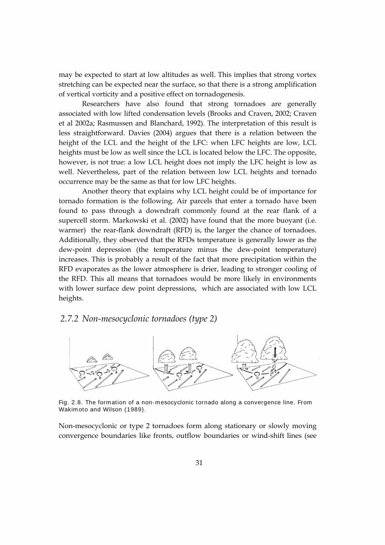
2.7.2 Non-mesocyclonic tornadoes (type 2)

Fig. 2.8. The formation of a non-mesocyclonic tornado along a convergence line. From Wakimoto and Wilson (1989).

Non-mesocyclonic or type 2 tornadoes form along stationary or slowly moving convergence boundaries like fronts, outflow boundaries or wind-shift lines (see

32

fig. 2.8.). Along these boundaries, a quasi-vertical vortex sheet may exist that may break up into individual vortices as a result of a horizontal shearing instability (Wakimoto and Wilson, 1989). The vortices can be stretched by convective updrafts located over the boundary and subsequently develop into tornadoes. Additionally, tilting of environmental horizontal vorticity may also play a role in generating vertical vorticity as it does in mesocyclonic tornadoes (Davies-Jones et al, 2001).

33

3. Datasets and methodology The goal of this study is to identify which values sounding-derived atmospheric parameters have in the neighborhood of severe convective weather events and thereby identify which physical processes are important for their formation.

In order to do that, it is necessary that we use measurements of these parameters very nearby both in space and time to reports of severe convective weather events. In other words, we need data from radiosondes released in the proximity of severe convective weather events. How to define the proximity of an event is a difficult issue that is addressed in section 3.4. Firstly, we will describe the data sets that were used in this study.

3.1 Severe convective weather events

The following severe convective weather events have been considered in this study...

• wind gusts having a speed of 25 m/s or more,

• tornadoes, including waterspouts (i.e. tornadoes over water)

• hail having a diameter of 2.0 cm or more in its longest direction

Unfortunately, a digital database of these types of events does not exist in the Netherlands, although the Dutch Meteorological Institute (KNMI) has archived data from the period of 1879 to 1965 (KNMI, 1879–1881, 1882–1887, 1888–1895, 1896–1965). Most of this data was too old to use in this study as radiosonde data was only available back to 1957. Considering that the frequency of radiosonde observations of stations in and around the Netherlands as well as the number of observations of severe weather has increased after 1975, we have decided to focus on that period.

The KNMI has kindly provided archived wind gust data of each station of the Dutch national operational measurement network. This data includes the maximum gust at each of the stations of the network and the hour at which this gust has occurred. A problem is that it is hard to find our which gusts were associated with convective storms. All gusts reported at stations located at least three kilometers from any coastline have been included in the analysis.

34

Additional data on both wind gusts and other severe weather types was obtained from the monthly magazine Weerspiegel of weather amateur organization VWK (Vereniging voor Weerkunde en Klimatologie). Data from this source was available to us since December 1975, the year in which Dutch weather enthusiasts established the VWK, then called "Werkgroep Weerkunde. The magazine Weerspiegel has been the primary source of data for this study. The time period considered in this study is 1-12-1975 to 31-08-2003 or 27 years and 10 months.

A few comments need to be made about the way amateur reports from Weerspiegel were incorporated in the data set used for this study, as some questions may arise about the quality of these reports. Firstly, wind measurements by weather amateurs will probably in general not reach the high level of quality of a professional measuring network. Most amateurs will likely not have a 10 m-long pole on which the sensor is mounted as is required by the World Meteorological Organization guidelines. The use of less expensive equipment will likely have a negative impact on the quality of the measurements as well. Nevertheless we have chosen to include amateur measurements to find instances on which the wind speed exceeded 25 m/s. When wind speeds of this force are occurring we reason that the local variability of the maximum wind speed (on a 100's of meters to kilometers scale) is probably of the same order of magnitude as the error of measurement, so that we would introduce only a small error by allowing for inclusion of measurements of somewhat poorer quality.

F-scale Damage description

F0 Some damage to chimneys; branches broken off trees; shallow-rooted trees pushed over; sign boards

F1 Peels surface off roofs; mobile homes pushed off foundations or overturned; moving autos blown off roads.

F2 Roofs torn off frame houses; mobile homes demolished; boxcars overturned; large trees snapped or uprooted; light-object missiles generated; cars lifted off ground.

F3 Roofs and some walls torn off well-constructed houses; trains overturned; most trees in forest uprooted; heavy cars lifted off the ground and thrown.

Table 3.1. The F-scale for tornado intensity (Fujita, 1971).

35

Fig. 3.1. Scheme depicting the guidelines that have been used for the categorization of tornado and wind events reported by weather amateurs.

Tornado observations of weather amateurs are another issue. It is possible that some observations by amateurs have been influenced by the wish of seeing a tornado rather than actual observations. Therefore we have been very critical with any mentioning of a tornado in the texts. Often, more details are provided by the observer than only the fact that a tornado was observed. Based on this contextual information we have made an assessment of its credibility. Of course this introduces quite some subjectivity. To reduce the subjectivity somewhat, a decision tree (fig. 3.1) has been used to determine whether the report should be listed as a tornado or not. It is possible that a few reports that are identified here as tornado reports are in fact shallow vortices along gust fronts, often referred to

36

as gustnadoes. We have made a distinction between tornadoes that occurred over land and over a water surface. We will call the latter waterspouts.

The F-scale classification (Fujita, 1971) has been done rather crudely. In some cases, the section in Weerspiegel provided F-scale assessments. We have followed these in most cases where available. In a few cases, the written damage description or photo material did not match the F-scale estimate. After a discussion with one of the current editors of the tornado section a handful of cases were reclassified. Nevertheless, the classification was likely not always correct. In assessing the F-scale classification, differences –noted by e.g. Dotzek (2000)– in structural strength between well-built houses in the United States and brick houses common in the Netherlands has been taken into account.

event type number of events

wind gusts >= 25 m/s 4056

hail (2.0-2.9 cm diameter) 78

hail (>2.9 cm diameter) 65

waterspouts 56

F0 tornadoes 36

F1 tornadoes 53

F2 tornadoes 7 F1 or stronger tornadoes

F3 tornadoes

61

1

Table 3-A. Severe weather events used in the analysis.

For this study it was important that both the time and location of the event were known with reasonable accuracy. Unfortunately this was not the case with all reports, which reduced the number of reports somewhat. Table 3-A shows the set of events that remained were used.

3.2 Radiosonde data

For this study we have used temperature, moisture and wind data from six stations in and around the Netherlands. In the table below the radiosonde data that were used are listed.

37

WMO-ID and name of station

period synoptic hours (GMT)

number number used*

06210 Valkenburg 01-07-2002 – 20–11-2002 402 375

06260 De Bilt 01-12-1975 – 27-04-1985 00, 12 32532 31372 28-04-1985 – 30-06-2002 00, 06, 12, 18 21-11-2002 – 31-08-2003

06447 Uccle 01-01-1990 – 31-08-2003 00, 12 9832 9675

10200 Emden 01-07-1997 – 31-08-2003 00, 12 4403 4377

10304 Meppen 02-01-1990 – 27-06-2003 occasionally at 12 1201 1185

10410 Essen 01-12-1975 – 31-08-2003 00, 12 19446 19381

total 67816 66365

Table 3-B. Overview of soundings used in the study. *see text.

The data sets contained data on temperature, mixing ratio, wind speed and wind direction at the standard pressure levels of 1000, 925, 850, 700, 500, 400, 300, 250, 200, 150, 125 and 100 hPa and at so-called significant levels between the standard levels, as well as at the earth's surface. Significant levels are extra levels with temperature and humidity and/or wind data so that the measured vertical profile of these variables can be reconstructed reasonably accurately by linearly interpolating between them. It is possible that some errors have been introduced by having data only at these selected levels. Better data were unfortunately not available.

For all soundings, all the studied parameters have been calculated. The first step was to interpolate (linearly with respect to height) the available data of temperature, mixing ratio, and u and v wind components at pressure levels spaced 1 hPa between the surface pressure and 100 hPa. Height data were interpolated assuming the hydrostatic equilibrium. Then, various shear-related parameters could directly be computed. Two parcel ascent curves Tp(p) were computed, namely that of

• a parcel having the average potential temperature and mixing ratio of the lowest 50 hPa's above the earth's surface (the 50 hPa mean parcel)

• the parcel having the highest θep in the lowest 500 hPa (most unstable or m.u.-parcel)

Additionally, the descent curve of the parcel having the lowest θep below the 500 hPa level was computed. The virtual temperature correction was applied to both the ascent and decent temperature curves and the environmental temperature

38

(Doswell and Rasmussen, 1994) to obtain a more accurate estimate of the parcel's thermal buoyancy.

Unphysical values for certain parameters occasionally resulted from the calculations as well as missing values. Missing values for parameters are the result of not all data being available to calculate them. It was not possible to inspect all the respective soundings individually to determine the causes of the unphysical values as a result of the large size of the dataset. A few soundings have however been inspected and the cause of the erroneous value was determined. In some cases, the original data was clearly incorrect while in a few cases an error in the calculation algorithm was discovered. In a few iterations the necessary corrections were made to the calculation program after reprocessing the entire set of soundings. After the last round of calculations 1451 soundings still contained unphysical values for at least one parameter. Those soundings were discarded from the analysis. The remaining numbers of soundings are given in the right column of table 3. These soundings include those for which not all parameters could be calculated.

3.3 Lightning data

In order to be able to classify soundings as thundery, data on the occurrence of lightning has been used that originated from the U.K. Met Office's Arrival-Time Difference System (Lee, 1986; Holt et al., 2001). This system makes use of the fact that lightning strikes produce radio waves called spherics, that move outward from the source at nearly the speed of light in all directions. The system consists of seven stations located in the UK, Gibraltar and Cyprus that precisely record the time at which spheric signals reach the station. By comparing the difference in time that spherics were recorded their sources can be fixed to an accuracy of less than 10 kilometers over West-central Europe. For this study, lightning recordings from 1 January 1990 to 31 December 1999 were available.

3.4 The definition of proximity

A difficult question in any study that uses proximity soundings, is to define what can be considered to be the "proximity" of a certain meteorological event. This problem has been addressed among others by Darkow(1969), Brooks et al. (1994), Rasmussen and Blanchard (1998).

39

If the criterion of proximity is very strict, the sample set will consist of soundings that represent the event's environment rather well, but in low numbers. If the criterion is chosen to be loose, a large sample set will result, that contains soundings some of which may not represent the storm's environment very well. The trick is to find some optimum in between. Definitions of proximity employed by the various authors differ strongly.

Darkow (1969), for example, required the sounding to be within 80 kilometers of the event and released within the time frame 45 minutes before to 60 minutes after the event. A somewhat subjective extra requirement that the sounding had sampled the same air-mass as that which entered the storm's inflow was additionally applied.

On the other extreme, Rasmussen and Blanchard (1998) allowed the sounding to be released within 400 kilometers of the event and in a time frame of three hours before to six hours after the event. An additional requirement was that soundings were located within a 150-degree-wide sector directed upstream of the event considering the boundary-layer mean wind. Other studies, like that of Thompson et al. (2002a) have employed numerical mesoscale models to get data that is believed to better resemble the proximity of a severe convective weather event than the closest available proximity sounding.

The number of severe weather reports used in the current study was rather small, so that the proximity criterion was not chosen to be very strict in order to retain a reasonable number of soundings associated with each particular type of severe weather. A maximum distance of 100 km from the sounding was thought to be a reasonable balance between the number of soundings and their representativity.

40

Fig. 3.2. Illustration of the proximity criterion: a sounding is a proximity sounding of an event if the event occurs within the 100 km radius circle around the point x(t0–4h) at time to–4h, or within the circle around the point x(t0–3h) at time to–3h, etc... x(t0) is the location where the sounding was released. Time t=t0 is 30 minutes before the official sounding time (see text).

To ascertain that the same air-mass that was sampled closely resembled that in which the event took place without having to inspect every sounding individually a proximity criterion was developed defined with respect to the moving air that was sampled by the radiosonde. This has been based upon the assumption that the rate of change of thermodynamic variables following an air parcel is smaller than the local rate of change of those variables. A complication is that air usually does not flow in the same direction and at the same speed at all altitudes in the atmosphere. Nevertheless, it was assumed that a proximity criterion defined with respect to a (virtual) moving parcel would be better than one defined with respect to the fixed location where the radiosonde was released. The following criterion was used:

41

A sounding is considered to be associated with an event when the event occurred within 100 km of a point advected with the mean wind from the sounding location at to.

where t0 is 30 minutes before the official time of the sounding, because the balloons are usually released some time before the official time in order to be completed at this time. So, for a 12 GMT sounding, t0 = 11:30 GMT. This criterion is illustrated in fig. 3.2.

The movement vector to choose for the parcel is related to the wind at different altitudes, but different movement vectors are chosen. It was investigated which movement vector resulted in the best proximity criterion. This quality of a proximity criterion was assessed by investigating the variance of a thunderstorm predictor among samples of soundings that were associated with thunderstorms when selecting them using that criterion. The best proximity criterion is that of which the set of selected soundings has the lowest variance of the predictor. This is because the set would only include soundings that have thundery values of the predictor associated with them. Where a less-than-optimal proximity criterion is used, soundings would be selected that were taken in environments non-supportive of thunderstorms, and were possibly associated with non-thundery values of the predictors. In that case the variance of the predictor values would be higher.

The 50-m.l.-Lifted Index was found to be a good predictor of thunderstorms in the HVD study and has been used for this purpose. The following criteria have been tested:

A sounding is considered to be associated with a thunder when at least one lightning strike was detected that occurred within 100 km of a point advected with the movement vector from the sounding location at t0 (see above).

where the movement vector was defined as

• the zero vector (no wind)

• the surface wind vector

• the 0–1 km A.G.L. density-weighted mean wind vector

• the 0–2 km A.G.L. density-weighted mean wind vector

• the 0–3 km A.G.L. density-weighted mean wind vector

• the 0–4 km A.G.L. density-weighted mean wind vector

• the 0–6 km A.G.L. density-weighted mean wind vector

42

X 0 1 2 3 4 6X 0 1 2 3 4 6 X 0 1 2 3 4 6 X 0 1 2 3 4 6 X 0 1 2 3 4 6 X 0 1 2 3 4 6

Fig. 3.3. Variance of the 50-hPa Lifted Index for the ensemble of soundings that were associated with thunderstorms according the criterion that at least one lightning strike was detected within 100 km of a point advected with the wind vector* from the sounding location. The wind vector* is the zero vector for the plots labeled with an X, the surface wind vector for those labeled with a 0, and the 0–1, 0–2, 0–3, 0–4, and 0–6 km A.G.L. mean wind vectors for those labeled respectively with a 1, 2, 3, 4 and 6. The whiskers show the 5% confidence interval. The six groups are for these cases in which we allowed for up to 1, 2, 3, 4, 5, and 6 hours absolute time difference between the sounding release and the detected lightning flash(es).

The results are shown in fig. 3.3 for the cases in which we allowed for 1, 2, 3, 4, 5 and 6 hours absolute time difference between the sounding release and the detection of lightning. It can be seen that the criterion using the zero wind vector is associated with a relatively high variance of the lifted index as is the criterion using the surface wind, especially as we allow for the absolute time difference to become larger. These are obviously not the best criteria. The 0–1 km, 0–2 km, 0–3 km, 0–4 km and 0–6 km mean wind vector criteria perform significantly better, especially when the time difference becomes larger. Of those five groups, the 0–3 km mean wind is perhaps slightly better than the other four criteria, although this is not statistically significant. We have therefore selected the 0–3 km wind criterion to be used in this study. We have also decided to consider only cases where the time of a severe weather event and a sounding release did not differ more than four hours (both before and after). Hence, the resulting criterion for proximity to a severe weather event that is as follows:

43

A sounding is considered to be associated with an event when the event occurred within 100 km of a point advected with the 0–3 km density-weighted mean wind from the sounding location (at t0).

This criterion is obviously not perfect. It does not ascertain that the same air-mass was sampled by the sounding as that in which the event took place. It is also likely that some of the soundings were released within convective updrafts or in nearby compensating downdrafts. Additionally, air at low altitudes may in some cases have originated from convective outflows. These effects have likely altered the calculated parameters significantly and negatively affected the representativity of the soundings relative to the unperturbed environment.

3.5 Categorization of the soundings

In order to test the value of parameters as predictors of severe convective weather and to be able to draw conclusions about the physical processes at work, we employed the following methodology.

All soundings have been put in one or more of the categories listed below based on whether they were proximity soundings of severe weather events as defined in the previous section. We have studied differences of the distributions of parameters between the various categories.

44

description abbreviation number of events

number of associated soundings

not associated with thunder or severe convective weather

NONE n/a 61168

associated with

thunder THUNDER n/a 2045

gusts ≥ 25 m/s WIND 4056 440

hail 2.0–2.9 cm * HAIL<3cm 78 52

hail > 2.9 cm * HAIL>=3cm 65 48

waterspouts WATER- SPOUT

56 35

an F0 tornado F0 36 25

an F1 tornado F1 53 39

an F2 tornado F2 8 6

an F1 or an F2 tornado** F1+ 61 45

not associated with severe weather and no lightning detection available. Not used in analysis

n/a n/a 4159

Table 3-C. The categorization of the soundings.

* This is the diameter of the largest hailstone that fell during a hail storm. Where it was reported that the hailstones were not round, the diameter considered was that in the stone's longest direction.

** Because of the very low number of the F2 tornado soundings (6), the

groups of F1 and F2 tornado soundings have been treated as one group (labeled F1+), except where parameter values differed significantly (at the 5% confidence level) between the two categories.

3.6 Climatological aspects of the severe weather events

Climatology is a reference state that forecasters need to keep in mind. Although not the primary goal of this study, we will briefly present some climatological data on severe convective events in the Netherlands.

45

3.6.1 Large hail

Fig. 3.4. The seasonal distribution of hail events.

The geographical distribution of the hail events is not very useful to study as many of the hail reports depicted occurred on the same days and the distribution over the country will probably be strongly biased towards those days. Therefore, it cannot be used to identify areas of higher or lower hail occurrence in a climatological sense.

Fig. 3.4 shows the distribution of hail events and the magnitude of hailstones over the year. It is seen that hail smaller than 3 cm occurs year-round, while larger hail seems to be a phenomenon exclusive to the summer season. Mind that some hail events, such as the three largest in June, have been reported on the same day (in this case June 6th, 1998).

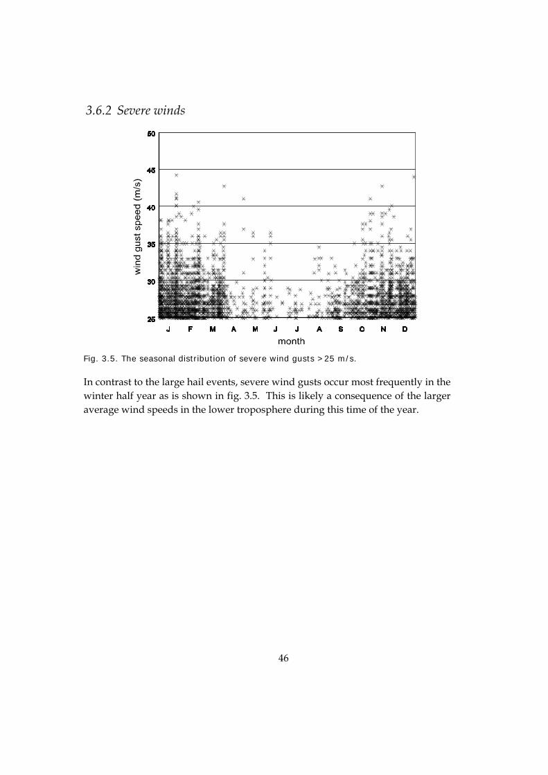
46

3.6.2 Severe winds

Fig. 3.5. The seasonal distribution of severe wind gusts >25 m/s.

In contrast to the large hail events, severe wind gusts occur most frequently in the winter half year as is shown in fig. 3.5. This is likely a consequence of the larger average wind speeds in the lower troposphere during this time of the year.

47

3.6.3 Tornadoes (and waterspouts)

Fig. 3.6. The geographical distribution of tornado events.

Fig. 3.7. The seasonal distribution of tornado events (including waterspouts).

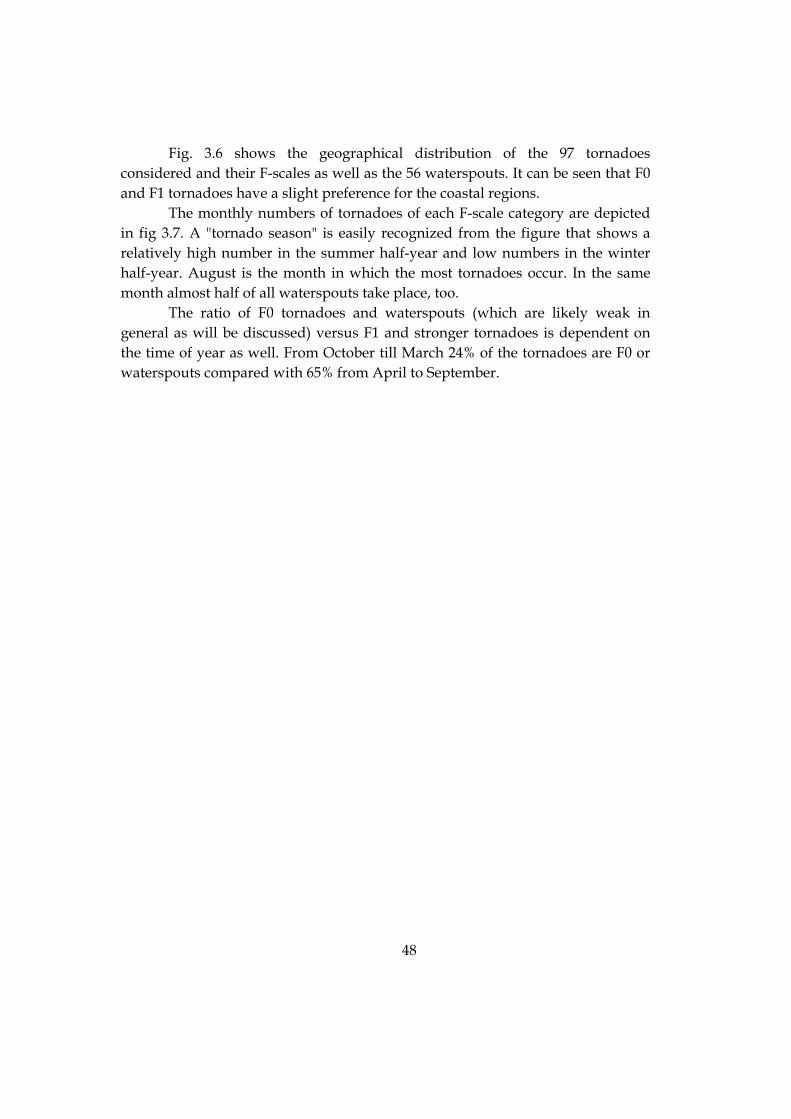
48

Fig. 3.6 shows the geographical distribution of the 97 tornadoes considered and their F-scales as well as the 56 waterspouts. It can be seen that F0 and F1 tornadoes have a slight preference for the coastal regions.

The monthly numbers of tornadoes of each F-scale category are depicted in fig 3.7. A "tornado season" is easily recognized from the figure that shows a relatively high number in the summer half-year and low numbers in the winter half-year. August is the month in which the most tornadoes occur. In the same month almost half of all waterspouts take place, too.

The ratio of F0 tornadoes and waterspouts (which are likely weak in general as will be discussed) versus F1 and stronger tornadoes is dependent on the time of year as well. From October till March 24% of the tornadoes are F0 or waterspouts compared with 65% from April to September.

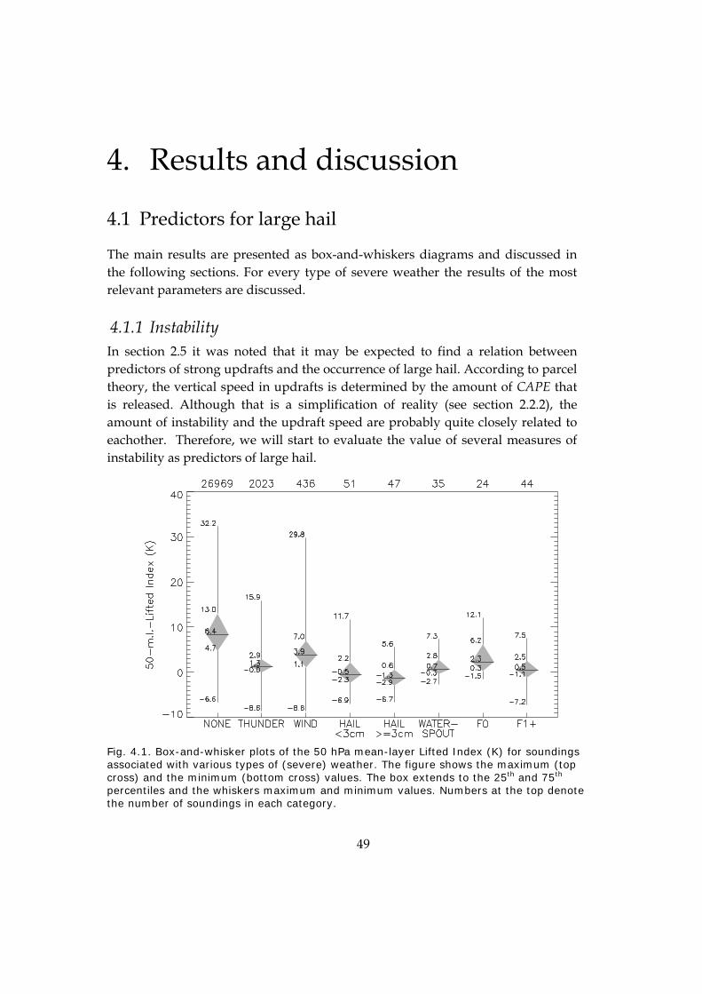
49

4. Results and discussion

4.1 Predictors for large hail

The main results are presented as box-and-whiskers diagrams and discussed in the following sections. For every type of severe weather the results of the most relevant parameters are discussed.

4.1.1 Instability In section 2.5 it was noted that it may be expected to find a relation between predictors of strong updrafts and the occurrence of large hail. According to parcel theory, the vertical speed in updrafts is determined by the amount of CAPE that is released. Although that is a simplification of reality (see section 2.2.2), the amount of instability and the updraft speed are probably quite closely related to eachother. Therefore, we will start to evaluate the value of several measures of instability as predictors of large hail.

Fig. 4.1. Box-and-whisker plots of the 50 hPa mean-layer Lifted Index (K) for soundings associated with various types of (severe) weather. The figure shows the maximum (top cross) and the minimum (bottom cross) values. The box extends to the 25th and 75th percentiles and the whiskers maximum and minimum values. Numbers at the top denote the number of soundings in each category.

50

Fig. 4.2. Box-and-whiskers plot of the most-unstable Lifted Index (K). Also see the explanation of fig. 4.1.

Fig. 4.3. Box-and-whiskers plot of the 50 hPa mean-layer CAPE (J/kg). Values very close to 0 J/kg are not shown. Also see the explanation of fig. 4.1.

51

Fig. 4.4. Box-and-whiskers plot of the most-unstable CAPE (J/kg). Values very close to 0 J/kg are not shown. Also see the explanation of fig. 4.1.

m.u-LI 50-m.l.-LI 50-m.l.-CAPE

m.u.-CAPE

hail (< 3.0 cm) vs. thunder

sig. at 1% sig. at 1% sig. at 1% sig. at 1%

hail (3.0 or larger) vs. thunder

sig. at 1% sig. at 1% sig. at 1% sig. at 1%

hail (< 3.0 cm) vs. hail (3.0 or larger)

sig. at 1% sig at 5% not sig sig. at 1%

Table 4-A. Significance of the difference of means of several parameters as determined with Student’s T-test with unequal variances assumed (Student, 1908; Research Systems Inc., 2004).

Figs. 4.1 to 4.4 show that both the Lifted Index of the most-unstable parcel and that of the 50 hPa mean-layer parcel are considerably lower and the respective amounts of CAPE larger with large hail events than with ordinary thunderstorms. Table 4-A shows that the means of all these parameters are significantly different between the groups of soundings associated with < 3.0 cm diameter hail and 3.0 cm or larger diameter on one hand and non-hail producing thunderstorms on the other hand (at the 1% confidence level). This is likely a result of the fact that updraft speeds need to be stronger to sustain large hailstones than the speeds required for sufficient charge-separation to cause lightning and thunder.

52

The figures show that the instability as measured with the CAPE and Lifted Index of the most-unstable parcel is larger with the category of hail > 3.0 cm than with hail of 2.0–2.9 cm diameter. The difference between the parameters calculated with the mean-layer parcel have a somewhat lower statistical significance (see Table 4-A) . Nevertheless, one can safely say that environments in which large hail take place are generally characterized by strong instability and that larger hail is on average associated with larger instability.

From figurs 4.1–4.4 it can be seen that the parameters based on the mixed-layer parcel qualitatively exhibit qualitatively the same differences between categories as do the most-unstable values. As the most-unstable parcel discriminates better between the < 3.0 cm hail and ≥ 3.0 cm hail categories, from here on only the most-unstable parcels will be considered.

4.1.2 Deep-layer shear Strong vertical wind shear generally enhances the degree of organization of storms. More organized storms tend to have longer lifetimes and allow hailstones to grow larger while particularly high shear over a deep layer enhances the chance of supercells (see also section 2.5.1). It may therefore be expected that the chance of large hail increases with increasing shear.

Fig. 4.5. Box-and-whiskers plot of the 0–6 km shear (m/s), here defined as the magnitude of the vector difference of the horizontal wind at 0 and 6 km. Also see the explanation of fig. 4.1.

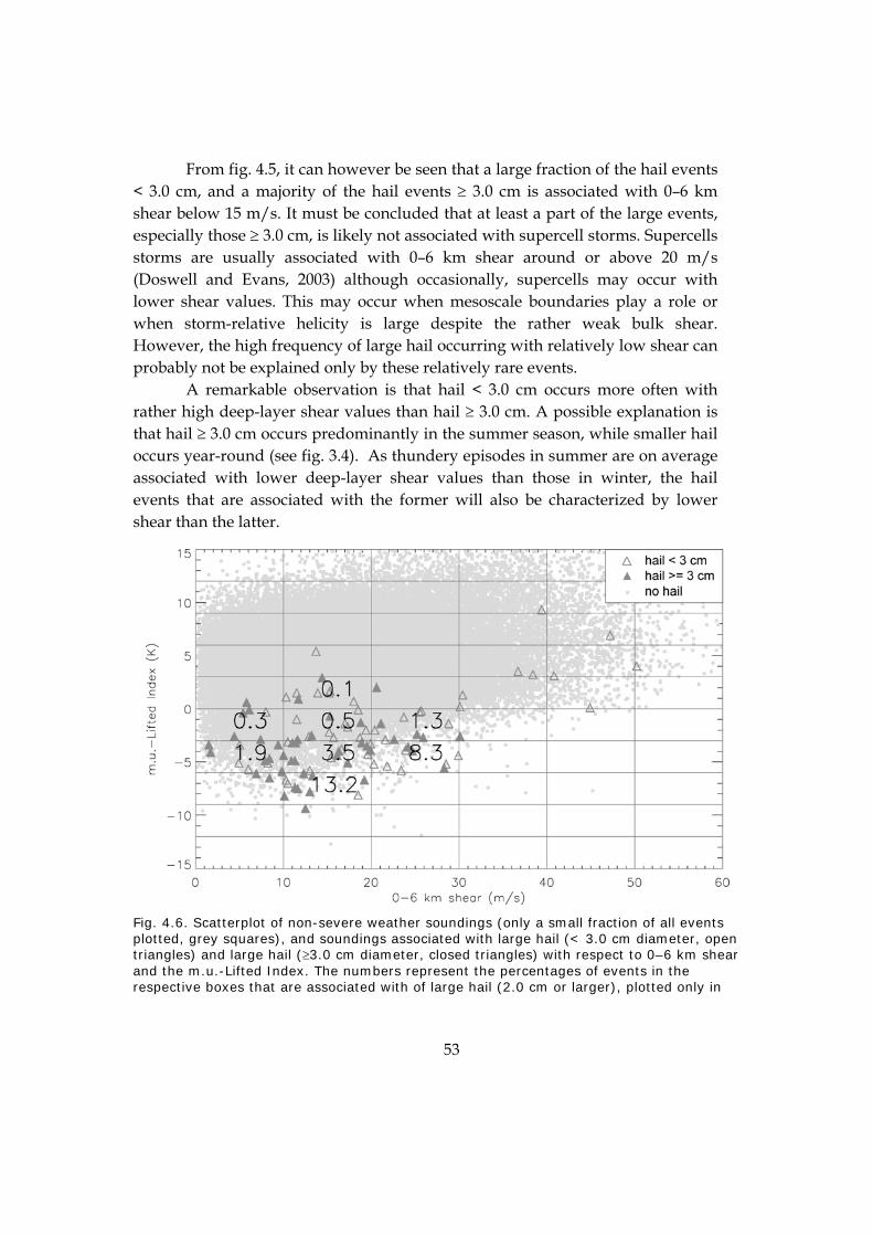
53

From fig. 4.5, it can however be seen that a large fraction of the hail events < 3.0 cm, and a majority of the hail events ≥ 3.0 cm is associated with 0–6 km shear below 15 m/s. It must be concluded that at least a part of the large events, especially those ≥ 3.0 cm, is likely not associated with supercell storms. Supercells storms are usually associated with 0–6 km shear around or above 20 m/s (Doswell and Evans, 2003) although occasionally, supercells may occur with lower shear values. This may occur when mesoscale boundaries play a role or when storm-relative helicity is large despite the rather weak bulk shear. However, the high frequency of large hail occurring with relatively low shear can probably not be explained only by these relatively rare events.

A remarkable observation is that hail < 3.0 cm occurs more often with rather high deep-layer shear values than hail ≥ 3.0 cm. A possible explanation is that hail ≥ 3.0 cm occurs predominantly in the summer season, while smaller hail occurs year-round (see fig. 3.4). As thundery episodes in summer are on average associated with lower deep-layer shear values than those in winter, the hail events that are associated with the former will also be characterized by lower shear than the latter.

Fig. 4.6. Scatterplot of non-severe weather soundings (only a small fraction of all events plotted, grey squares), and soundings associated with large hail (< 3.0 cm diameter, open triangles) and large hail (≥3.0 cm diameter, closed triangles) with respect to 0–6 km shear and the m.u.-Lifted Index. The numbers represent the percentages of events in the respective boxes that are associated with of large hail (2.0 cm or larger), plotted only in

54

boxes containing more than 5 hail events. Note that only a fraction of large hail events that occurred have been reported.

One may ask if the finding that the events of very large hailstones on average occur in rather weakly sheared environments is in contradiction with the idea that large hail is favored by strong deep layer shear. This is not the case. The rarity of large hail events is merely caused by the fact large shear combined with large instability is very rare in the Netherlands. When the density of the large hail events in shear/instability space is normalized by the density of all events, we get a different picture. Fig 4.6 shows the percentage of the total number of events (i.e. thundery and non-thundery) per box that were associated with hail. Especially the boxes bounded by the –3 and –6 K lines of m.u.-Lifted Index show a strong increase of the hail occurrence with increasing shear, so that the relative frequency of large hail does in fact strongly increase with increasing shear.

It is important to realize that fig 4.6 probably does not show the true ratio of hail events versus all events as the occurrence of large hail was (possibly strongly) underestimated, i.e. not all large hail that occurred was reported. Hence, the numbers in the figure should be interpreted in a qualitative sense: the true percentages could be several times higher.

4.1.3 Low-level moisture and the wet-bulb zero level Not all thunderstorms that occur in environments of large instability produce large hail. In addition to instability and shear there are a number of other parameters that have skill in distinguishing hail soundings from thundery soundings.

55

Fig. 4.7. As fig. 4.6, but now for the most-unstable Lifted Index and the 0–1 km average mixing ratio.

The relation between low-level moisture and large hail occurrence is illustrated by fig. 4.7. It follows that a higher absolute moisture content of the air in the 0–1 km A.G.L. layer is associated with an increase of the chance of large hail at the same level of instability. The most likely explanation is given by the faster accretion of hailstones in an updraft containing large quantities of liquid water, which only occurs when the water vapor content of the air entering the updraft is large.

In the United States, the height at which the wet-bulb temperature (Tw) is 0 °C is occasionally used as a hail predictor. However, Edwards and Thompson (1998) note that this quantity has little skill in estimating hail size. Thereby, it may not be a useful predictor of large hail in general. Still, we have explored if this parameter has any predicting value.

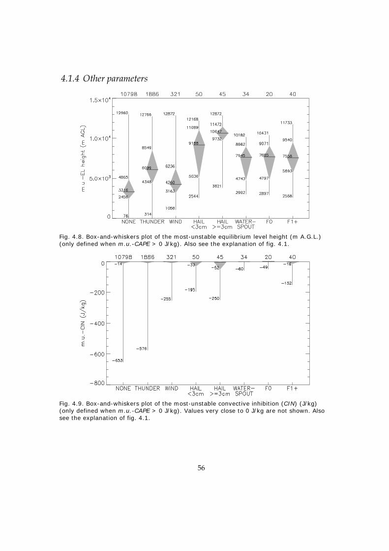
56

4.1.4 Other parameters

Fig. 4.8. Box-and-whiskers plot of the most-unstable equilibrium level height (m A.G.L.) (only defined when m.u.-CAPE > 0 J/kg). Also see the explanation of fig. 4.1.

Fig. 4.9. Box-and-whiskers plot of the most-unstable convective inhibition (CIN) (J/kg) (only defined when m.u.-CAPE > 0 J/kg). Values very close to 0 J/kg are not shown. Also see the explanation of fig. 4.1.

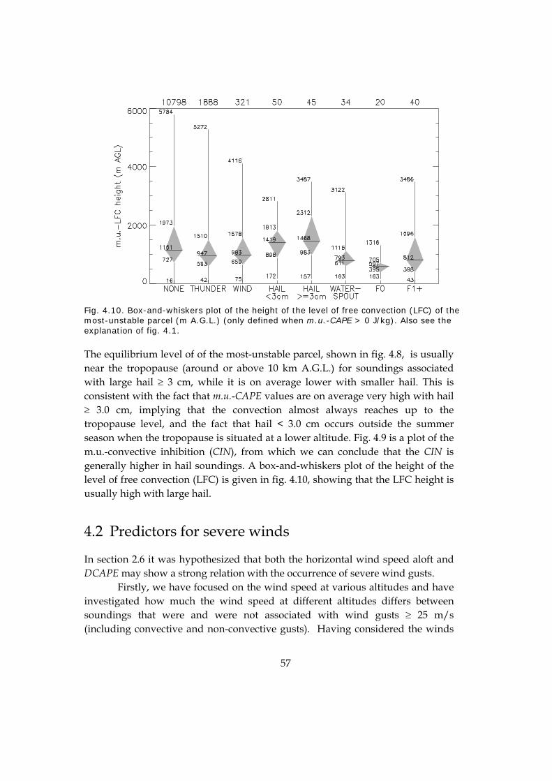
57

Fig. 4.10. Box-and-whiskers plot of the height of the level of free convection (LFC) of the most-unstable parcel (m A.G.L.) (only defined when m.u.-CAPE > 0 J/kg). Also see the explanation of fig. 4.1.

The equilibrium level of of the most-unstable parcel, shown in fig. 4.8, is usually near the tropopause (around or above 10 km A.G.L.) for soundings associated with large hail ≥ 3 cm, while it is on average lower with smaller hail. This is consistent with the fact that m.u.-CAPE values are on average very high with hail ≥ 3.0 cm, implying that the convection almost always reaches up to the tropopause level, and the fact that hail < 3.0 cm occurs outside the summer season when the tropopause is situated at a lower altitude. Fig. 4.9 is a plot of the m.u.-convective inhibition (CIN), from which we can conclude that the CIN is generally higher in hail soundings. A box-and-whiskers plot of the height of the level of free convection (LFC) is given in fig. 4.10, showing that the LFC height is usually high with large hail.

4.2 Predictors for severe winds

In section 2.6 it was hypothesized that both the horizontal wind speed aloft and DCAPE may show a strong relation with the occurrence of severe wind gusts.

Firstly, we have focused on the wind speed at various altitudes and have investigated how much the wind speed at different altitudes differs between soundings that were and were not associated with wind gusts ≥ 25 m/s (including convective and non-convective gusts). Having considered the winds

58

at the surface (i.e. 10 m), 500 m, 1 km, 1.5 km, 2 km, 3 km, 4 km, 5 km and 6 km A.G.L., this difference was most significant for the 2 km wind.

wind at wind speed

from soundings near severe wind gusts

wind speed from soundings not near severe wind gusts

t-test statistic for independent samples with sample size 436

10 m 8.1 3.7 26.5

500 m 19.6 9.0 28.7

1 km 23.9 10.0 31.9

1.5 km 25.2 10.4 33.7

2 km 25.5 10.9 34.6

3 km 26.9 12.3 34.2

4 km 29.1 14.0 31.5

5 km 31.6 15.9 28.0

6 km 35.0 18.1 25.3

Table 4-B. Test results of Student's t-test for the difference between the means of thw winds among the groups of soundings that were associated and not associated with severe wind gusts. The higher the test statistic, the higher the significance of the difference (all values in the table are highly significant).

Table 4-B shows the results of this analysis that was done using Students' t-test for independent samples not assuming equal variances. The higher the t-test statistic, the more significant the difference. It turns out that the wind at 2 km altitude is more strongly related to the occurrence of severe wind gusts ≥ 25 m/s than the wind at higher and at lower altitudes.

59

Fig. 4.11. Scatterplot of all wind events (V's) and all other soundings (squares) with respect to DCAPE and 2 km A.G.L. wind speed. Numbers denote the percentage of soundings associated with a wind event in each box.

If downward transport of horizontal momentum were not important, one would expect the wind at 10 m A.G.L. –where the gusts are measured– to be the most strongly related to the occurrence of strong gusts. That fact that not the 10 m A.G.L. wind, but the wind at 2 km A.G.L. is the strongest related suggests that this process is probably important.

Secondly, the value of DCAPE as a predictor of severe wind gusts has been assessed. A scatterplot of all events with respect to the 2 km A.G.L. wind and DCAPE has been constructed in fig. 4.11. It can be seen that indeed most wind events are associated with a high 2 km wind. Some wind events, however, occurred with much lower shear.

It can be seen that the likelihood of severe gusts increases rapidly where the 2 km wind exceeds 30 m/s. With weaker 2 km winds, the chance of severe gusts increases as DCAPE becomes very high (note the percentages in the 10-20 m/s column, that increase with increasing DCAPE). These events are probably associated with thunderstorms that produce strong outflows. This explains why the likelihood of severe gusts does not increase as strongly with increasing DCAPE as with increasing 2 km winds: the gusts primarily forced by DCAPE require thunderstorms, that may not occur even though DCAPE large (e.g.

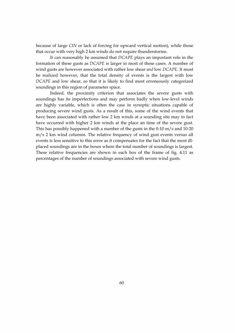
60

because of large CIN or lack of forcing for upward vertical motion), while those that occur with very high 2 km winds do not require thunderstorms.

It can reasonably be assumed that DCAPE plays an important role in the formation of these gusts as DCAPE is larger in most of these cases. A number of wind gusts are however associated with rather low shear and low DCAPE. It must be realized however, that the total density of events is the largest with low DCAPE and low shear, so that it is likely to find most erroneously categorized soundings in this region of parameter space.

Indeed, the proximity criterion that associates the severe gusts with soundings has its imperfections and may perform badly when low-level winds are highly variable, which is often the case in synoptic situations capable of producing severe wind gusts. As a result of this, some of the wind events that have been associated with rather low 2 km winds at a sounding site may in fact have occurred with higher 2 km winds at the place an time of the severe gust. This has possibly happened with a number of the gusts in the 0-10 m/s and 10-20 m/s 2 km wind columns. The relative frequency of wind gust events versus all events is less sensitive to this error as it compensates for the fact that the most ill-placed soundings are in the boxes where the total number of soundings is largest. These relative frequencies are shown in each box of the frame of fig. 4.11 as percentages of the number of soundings associated with severe wind gusts.

61

Fig. 4.12. Scatterplot of all wind events (v's) and all other soundings (squares) with respect to m.u.-CAPE (quadratic scale) and 2 km A.G.L. wind speed. Numbers denote the percentage of soundings associated with a wind event in each box.

It has now been found that DCAPE indeed has some values as a predictor of severe gusts in situations of weak low-level winds. DCAPE is closely correlated with CAPE, although it does not depend on low-level moisture like CAPE and, unlike CAPE, depends on mid-level moisture (i.e. at the level where downdrafts originate). It has been investigated whether it is possible to determine any added value of DCAPE over CAPE in predicting convective wind gusts.

A look at fig. 4.12, which is similar to fig 4.11. but with m.u.-CAPE along the vertical axis, reveals that wind events are very similarly distributed compared with DCAPE. Looking at the events with weak to moderate lower tropospheric winds (wind at 2 km < 20 m/s), it does not become clear that DCAPE is better than m.u.-CAPE.

4.3 Predictors for tornadoes

Now parameters will be discussed that potentially have skill to distinguish tornadic environments from non-tornadic environments.

62

4.3.1 Instability and Level of Free Convection

Fig. 4.13. Box-and-whiskers plot of 0–3 km CAPE (J/kg). Also see the explanation of fig. 4.1.

Firstly the results of parameters measuring instability are discussed. From figs. 4.1–4.4 it follows that the distribution of LI and CAPE with waterspouts, weak (F0), and stronger (F1+) tornadoes is quite similar to the distribution with thunderstorms in general. Those parameters are therefore not very useful for forecasting tornadoes in environments supportive of thunderstorms.

The Lifted Index in particular may give a misleading signal about the available instability. As the equilibrium level is occasionally located below the 500 hPa level (see fig. 4.8) –the level at which the Lifted Index evaluates the parcel’s thermal buoyancy– it is sometimes positive while the parcel does in fact have positive thermal buoyancy below this level.

Alternatively, the m.u.-CAPE released below 3 km (Davies, 2002) seems to be a more valuable parameter for tornado forecasting. This low-level CAPE parameter is significantly higher with waterspouts and weak tornadoes compared with thunderstorms. With stronger F1+ tornadoes, the distribution is quite similar to that associated with thunderstorms on average. Low-level CAPE is probably associated with strong upward accelerations within updrafts close to the earth's surface that amplifies vertical vorticity by stretching. The same effect may be reflected in the tendency of tornadoes to occur with low LFC heights, which is shown in fig. 4.10.

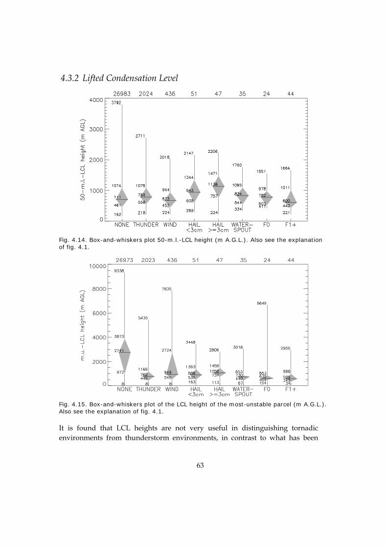
63

4.3.2 Lifted Condensation Level

Fig. 4.14. Box-and-whiskers plot 50-m.l.-LCL height (m A.G.L.). Also see the explanation of fig. 4.1.

Fig. 4.15. Box-and-whiskers plot of the LCL height of the most-unstable parcel (m A.G.L.). Also see the explanation of fig. 4.1.

It is found that LCL heights are not very useful in distinguishing tornadic environments from thunderstorm environments, in contrast to what has been

64

found in various U.S.-based studies (Craven et al., 2002a; Brooks and Craven, 2002). Figs 4.14 and 4.15 show that the 50-m.l.-LCL heights are rather low with tornadoes: significantly lower than the situations of large hail, but there is no significant difference of 50-m.l.-LCL heights between the categories of waterspouts or weak tornadoes on one hand and thunderstorms on the other hand. Only the difference in LCL height between F1+ tornadoes and thunderstorms is statistically significant at the 1% confidence level. Nevertheless, the interquartile ranges between those categories show a very large overlap and the thunderstorm category is much larger. This means that in a given operational forecast situation the difference is of little value. It seems that in contrast to much of the United States, the majority of thunderstorm events in the Netherlands occur with low LCL heights, so that LCL height is in general not as much a limiting factor for the development of tornadoes in the Netherlands as it is in much of the U.S.A.

Some very high LCL heights above 5000 m A.G.L. are shown in fig. 4.15. These are no errors, but due to the fact that the parcel with the highest equivalent potential temperature θe in the lowest 3000 m A.G.L. –the level of origin of the most-unstable parcel according to the definition used in this study– was located in a dry and warm subsidence inversion and not in the convective layer.

4.3.3 Wind shear

Fig. 4.16. Box-and-whiskers plot of the 0–1 km A.G.L. shear (m A.G.L.). Also see the explanation of fig. 4.1.

65

Wind shear appears to be rather promising parameter for tornado forecasting. An important observation visible in fig 4.16 is that the 0–1 km wind shear with of F1 and F2 tornadoes is stronger than with F0 tornadoes and thunderstorms. With F0 tornadoes, the wind shear is lower than on average with thunderstorms. This suggests that the process responsible for their formation, the rolling up of vortex-sheets, may be inhibited by strong low-level wind shear. It is possible that strong turbulence in the boundary layer that is associated with the strong wind shear either disrupts the formation of well-defined vortex sheets or disrupts the rolling-up into separate vortices.

In contrast to most likely non-mesocyclonic F0 tornadoes, the F1 and F2 tornadoes that supposedly are partly mesocyclonic, require strong wind shear to form. It is striking to see that low-level shear strongly increases with the intensity of the tornadoes.

Considering the shear distribution of the waterspout events, it seems that this category –of which no intensity estimates exist– consists mostly of the weaker, non-mesocyclonic tornadoes, while a few events are associated with shear values more typical of the stronger, possible mesocyclonic tornadoes.

Fig 4.17. Scatterplot of non-severe weather events (only a small fraction of all events plotted, grey squares), and events of waterspouts (closed grey triangles) and F0 (open black triangles) and stronger tornadoes (closed black triangles) with respect to 0–1 km shear (m/s) and the m.u.-Lifted Index (K).

66

Fig. 4.17 shows the various event types as a scatterplot with respect to the 0–1 km shear and the m.u.-Lifted Index. The figure illustrates well the aforementioned observation of stronger tornadoes occurring with stronger 0–1 km shear. More precisely, it seems that a line drawn at 7 m/s separates the F1+ tornadoes from the F0 tornadoes quite well. Most waterspouts fall on the low shear side of the line. The figure shows the high lifted indicesthat are occasionally associated with F0 tornadoes in cases of shallow instability.

The 0–6 km, or deep-layer shear (fig. 4.5) –that strongly influences the process of storms organizing into multicells or supercells– has a much less clear distinction between the F0 and F1 tornadoes. However, F2 tornadoes are associated with significantly (at the 1% confidence level) stronger shear than the F0 and F1.

Fig. 4.18. Box-and-whiskers plot of the 0–3 km storm-relative helicity (m2/s2). Also see the explanation of fig. 4.1.

67

Fig. 4.19. Box-and-whiskers plot of the 0–1 km storm-relative helicity (m2/s2). Also see the explanation of fig. 4.1.

In addition to the 0–1 km and 0–6 km bulk shear, storm-relative helicity was tested as a possible predictor for tornadoes. Box-and-whiskers plots of the storm-relative helicity in the 0–1 km and 0–3 km A.G.L. layers are presented in figs. 4.18 and 4.19. The figures show that both helicity values are high in environments of strong wind gusts and with F1 and –especially– with F2 tornadoes. For F0 tornadoes or hail, the distributions are centered just above 0 m2/s2 and category and are not significantly different from the NONE and THUNDER categories. The fact that high SRH values are observed with F2 tornadoes appears to be promising, but must however be recognized that the WIND category consist of many more events than the F2 category. This means that if one would decide always to forecast tornadoes when, for example, 0-1 km SRH in excess of 196 m2/s2 is observed (which is the median value for F2 tornadoes), this would result in a very high false alarm ratio.

68

4.4 Average profiles for each severe weather type

a. THUNDER b. SMALL HAIL

c. LARGE HAIL d. F1+

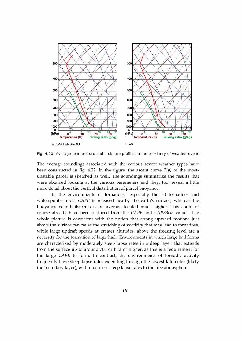
69

e. WATERSPOUT f. F0

Fig. 4.20. Average temperature and moisture profiles in the proximity of weather events.

The average soundings associated with the various severe weather types have been constructed in fig. 4.22. In the figure, the ascent curve T(p) of the most-unstable parcel is sketched as well. The soundings summarize the results that were obtained looking at the various parameters and they, too, reveal a little more detail about the vertical distribution of parcel buoyancy.

In the environments of tornadoes –especially the F0 tornadoes and waterspouts– most CAPE is released nearby the earth's surface, whereas the buoyancy near hailstorms is on average located much higher. This could of course already have been deduced from the CAPE and CAPE3km values. The whole picture is consistent with the notion that strong upward motions just above the surface can cause the stretching of vorticity that may lead to tornadoes, while large updraft speeds at greater altitudes, above the freezing level are a necessity for the formation of large hail. Environments in which large hail forms are characterized by moderately steep lapse rates in a deep layer, that extends from the surface up to around 700 or hPa or higher, as this is a requirement for the large CAPE to form. In contrast, the environments of tornadic activity frequently have steep lapse rates extending through the lowest kilometer (likely the boundary layer), with much less steep lapse rates in the free atmosphere.

70

Another observation is that with F1+ tornadoes the CAPE is not very high and the sounding looks not too exceptional at all, although F1+ tornadoes are quite rare. Probably the kinematics of the wind field –which are not shown in 4.22– are a more important factor for the formation of these tornadoes than the thermodynamics. This finding is illustrated by the identification of 0-1 km shear being a better predictor of F1+ tornadoes than any thermodynamic parameter.

71

5. Conclusions

5.1 Summary of findings

5.1.1 Characterization of severe weather environments

LARGE HAIL Large hail occurs year-round, but is more frequent in summer. Hailstones of 3.0 cm diameter or larger occur exclusively in the summer half-year.

Hail occurrence is closely related to the amount of CAPE that is present. The Lifted Index can be used as a proxy for CAPE. Hail with a diameter of ≥ 3.0 cm occurs typically with around 1000 J/kg m.u.-CAPE and a m.u.-LI of –4. Smaller hailstones are occasionally associated with much lower instability.

Wind shear in the 0-6 km layer is much higher with the smaller hail events (18.5 m/s) than with the larger hail events (12.3 m/s). The main reason is thought to be that a fraction of the smaller hail events occurs in the winter half-year in which the deep-layer wind shear is stronger on average. The typical storm type occurring with high deep-layer shear and low instability, that is still able to produce very strong updrafts to allow for hail formation is the low-topped or mini-supercell. This is likely the storm type responsible for many of the smaller-hail events, especially those that occur with relatively small CAPE. In contrast, most of the cases of hail ≥ 3.0 cm are probably associated with multicell convection as 12.3 m/s 0–6 km shear is generally not sufficient to sustain supercells. Strong vertical motion is however possible in those storms because of the large amounts of CAPE. It was found that, although the majority of events of hail ≥ 3.0 cm occcurred with shear values typical for multicells, the chance of large hail strongly increases with increasing 0–6 km shear.

Consistent with what was discussed above, the m.u.-equilibrium level –a proxy for the height of the storm tops– was found to be typically in the 9–13 km range for the very large (> 3.0 cm) hail cases, while it was often lower for smaller hail.

Another important factor for the formation of hail ≥ 3.0 is likely the availability of large amounts of moisture. It was found that with equal amounts of instability, the chance of large hail increases when the 0–1 km average mixing

72

ratio increases. Typically the average 0–1 km average mixing ration exceeds 8.0 g/kg for cases of hail ≥ 3.0 cm.

WIND GUSTS ≥ 25.0 m/s Wind gusts ≥ 25.0 are most frequent in the winter half-year. They occur often with strong winds in the lower troposphere (but not necessarily at the surface), suggesting the downward transport of strong horizontal winds speeds to the surface is an important process for the formation of severe gusts. In most cases, DCAPE is low, which suggests that the vertical momentum developing in downdrafts is of lesser importance for the final wind gust speed than the horizontal momentum the decending air already contained.

Occasionally, however, strong gusts occur with low 2 km winds. This is often in combination with high DCAPE and CAPE values, suggesting that downdrafts produced by strong deep convection sometimes produces strong gusts in absence of strong horizontal winds. It was surprisingly not found that DCAPE was a better predictor of this type of gusts than m.u.-CAPE.

TORNADOES Weak tornadoes occur most frequently from May to September and near the coast. Weak (F0) tornadoes occur with lower than average low level (0-1 km) shear (average: 7.0 m/s, average F0: 4.4 m/s), while stronger tornadoes occur with much higher than average low-level shear (average F1: 9.0 m/s , F2: 20.3 m/s). 0-6 km shear increases only, albeit strongly, when going from the F1 to the F2 categories (increasing from 15 to 27 m/s). All this suggests that the weaker tornadoes are probably non-mesocyclonic, as the development of mesocyclones is associated with strong vertical wind shear. However, the stronger (F1 and F2) tornadoes do probably include mesocyclone-related tornadoes. Most waterspouts fit well into the category of F0 tornadoes and are probably of the same (non-mesocyclonic) type.

On average m.u.-CAPE in tornadic cases is similar to that in any thunderstorm case, so that it is not an important parameter for forecasting tornadoes. The weak (F0) tornadoes are associated with with high m.u.-CAPE released below 3 km, typically 100–300 J/kg. This is not as much the case for stronger tornadoes that often have CAPE3km values around 100 J/kg, which is typical of any convective situation.

73

All tornadic (weak or strong) environments are typically characterized by having no CIN and low LFC and LCL heights. The low LFC height differs most significantly between the categories of thunderstorms and F0 tornadoes, while the low LCL height is differs most significantly between thunderstorms and F1+ tornadoes. LFC and LCL heights probably have limited value for forecasting tornadoes.

The equilibrium level (and by approximation storm tops) are usually found around 7.5 km A.G.L. with F1 and F2 tornadoes, but occasionally (much) lower especially with F0 tornadoes and waterspouts.

5.1.2 Implications of the results for forecasting The relation between certain parameters and types of severe weather has only be established in a qualitative sense. The fact that only a low fraction of all severe events that occurred were reported in the period that was studied has prevented us form making an quantitative estimate of the probability of a severe weather event occurring in association with a sounding in a certain area of parameter space. Instead only qualitative statements have been given above like "the chance of hail increases with increasing shear" without stating how large the chance of hail really is with a certain amount of shear. Similarly, it has not been possible, for example, to define an area in parameter space in which the chance of tornadoes is so large that a warning for tornadoes should immediately be given. Forecasters should use these results accordingly and use them in combination with other available information when making forecasts and nowcasts. The best way of using the above results is probably to monitor whether parameters are in the range supportive of a certain event type or are extreme in the context of climatology. This should create the awareness that certain types of severe weather may occur, without directly warranting a warning. For example, when m.u.-CAPE of 2000 J/kg has been observed and 0–6 km shear is in excess of 10 m/s this should make forecasters aware of the fact that large hail may occur within the next hours, even though it is more likely that this will not be the case. Depending on whether storms are indeed forecast to develop and other factors a forecaster needs to consider, it can be decided if a warning for large hail is indeed warranted.

5.1.3 Improving forecasting The likelihood of severe weather is influenced by factors that cannot be assessed using radiosonde soundings. These include, most importantly, processes that initiate thunderstorms (rising motions on various scales). The synoptic context

74

can give additional information to forecasters in this respect. Additionally, radar data can give information on which storm types are occurring and can give a clue which storm types will affect the area of interest in the near future. Insight in the physical processes at work on the scale of storms and storm systems are of considerable value to forecasters. More work, possibly in the form of conceptual models, case-studies and other educational material focused on convective storms will probably be beneficial for severe storm forecasting in the Netherlands.

5.2 Suggestions for further research

5.2.1 Severe weather observations Future studies that use data of more severe weather observations may allow us to make quantitative estimates of severe weather probabilities instead of qualitative. But it is crucial that more of the severe weather that occurs is reported. A more structural way of collecting and storing reports than that of an amateur meteorological organization, how valuable though is has proven to be, is necessary. Reports of amateurs will however remain of high importance as conventional measuring networks do not have the resolution, nor are designed for the observation of tornadoes, large hail and very local wind gusts. It is preferred to use an international approach in order to get large quantities of observational data and international cooperation between experts that can validate the reports so that the data has a high level of quality. An initiative in this direction in Europe is currently being initiated under the name European Severe Weather Database (ESWD) (Groenemeijer et al, 2004). National meteorological services (NMS's) will validate reports for their country, while the network is pan-European. It makes use of the possibilities of the internet to share the information internationally and receive reports from weather amateurs, that may be organized in national or regional networks.

5.2.2 Climate change and the frequency of convective severe weather If qualitative estimates of the chance of various types of severe weather in parameter space can be obtained, this can help to answer the frequently-asked question: "What will be the effects of climate change on the frequency of severe weather events.", at least with respect to convective weather events. Using data from numerical climate simulation models one can study of parameters will more or less frequently have values associated with a high chance of a certain type of

75

severe weather. To be more concrete three questions will probably be most important

• Which parameters are of relevant to the severe weather events? (this question was addressed in this study)

• What is the probability of a particular severe weather event occurring with each area of parameter space? (i.e. a question considered in this study, but then to be answered quantitatively)

• What are the systematic errors of the climate model in predicting the parameters?

• When correcting for these systematic errors, what does the climate model predict to be the probability of each parameter to have a particular value?

• How does this translate to the frequency of severe weather events considering the answers to question 2?

5.2.3 Use of better or more radiosonde data Numerical models can probably not only be of use in assessing the effects of climate change but also in answering questions 1 and 2 (above). Operational numerical models of high resolution can probably come in useful when trying to find the values of the relevant parameters in the immediate proximity of severe weather events, as has been done already by Thompson et al. (2002a, 2003) . This may help to increase the size of the data set as operational mesoscale model data is usually available of all times since the development of the model and of all locations in its domain, while an actual radiosonde sounding may not be available. An alternative, that has not been used herein, that is less good but does not require the use of a mesoscale model is to adjust the low-level part of each sounding using information from nearby surface data before calculating the parameters.

76

Acknowledgements I would like to thank several people who have contributed to this study. Firstly, Aarnout van Delden has supervised me during this M.S. thesis and I would like to thank him for this.

Additionally, thanks should go to Marc Allaart of the Dutch Meteorological Institute (KNMI) who has kindly helped providing radiosonde data for the Dutch stations from the KNMI archive. Archived data from the Dutch operational measurement network was kindly provided, too, by the KNMI. The Deutscher Wetterdienst (DWD) and the Royal Meteorological Institute of Belgium (RMI) have provided radiosonde data used in this study as well. The U.K. Meteorological Office have provided the SFLOC lightning data that were used. I want to thank the Dutch Meteorological and Climatological Association (VWK), its observers and especially the editors of the sections on thunderstorms and on tornadoes in the magazine Weerspiegel since 1976, as most severe weather data originated from their articles.

Alwin Haklander has indirectly assisted me in writing this thesis with writing an inspiring M.S. thesis himself that was often consulted while writing this report. I have had some nice discussions about the study with Oscar van der Velde (CNRM, Toulouse), Jeroen van Zomeren (IMAU, Utrecht) and Nick Verge. With John Teunissen and Bernard Hulshof I have had some discussion about the F-rating of certain tornado cases. To conclude, thanks to Karel Holvoet and John Kambeel for allowing me to use photo material. Thank you all!

Pieter Groenemeijer, Utrecht, February 8th, 2005.

77

References Bolton, D., 1980: The computation of equivalent potential temperature. Mon. Wea.

Rev., 108, 1046–1053.

Boyden, C. J., 1963: A simple instability index for use as a synoptic parameter. Meteor. Mag., 92, 198–210.

Brooks, H. E., and J. P. Craven, 2002: A database of proximity soundings for significant severe thunderstorms, 1957–1993. Preprints, 21st Conference on Severe Local Storms, San Antonio, Texas, American Meteorological Society, 639–642.

Bunkers, M. J., B. A. Klimowski, J. W. Zeitler, R. L. Thompson, M. L. Weisman, 2000: Predicting supercell motion using a new hodograph technique. Wea. Forecasting, 15, 61–79.

Byers, H. R. and R. R. Braham Jr., 1949: The Thunderstorm. U.S Government Printing Office, Washington D.C., 287 p.p.

Carbone, R. E., 1982: A severe frontal rainband. Part I: stormwide hydrodynamic structure. J. Atmos. Sci., 39, 258–279.

Carbone, R. E., 1983: A severe frontal rainband. Part II: Tornado Parent Vortex Circulation. J. Atmos. Sci., 40, 2639–2654.

Craven, J. P., H. E. Brooks, and J. A. Hart, 2002a: Baseline climatology of sounding derived parameters associated with deep, moist convection. Preprints, 21st Conference on Severe Local Storms, San Antonio, Texas, American Meteorological Society, 643–646.

Craven, J. P., R. E. Jewell, and H. E. Brooks, 2002b: Comparison between observed convective cloud-base heights and lifting condensation level for two different lifted parcels. Wea. Forecasting, 17, 885–890.

Darkow, G. L., 1969: An analysis of over sixty tornado proximity soundings. Preprints, 6th Conf. Severe Local Storms (Chicago, IL), Amer. Met. Soc, 218–222.

78

Davies-Jones, R., 1984: Streamwise vorticity: the origin of updraft rotation in supercell storms. J. Atm. Sci., 41, No. 20, 2991–3006.

Davies-Jones, R., R. J. Trapp and H.B. Bluestein, 2001: Tornadoes and tornadic storms. In Severe Convective Storms, C. A. Doswell III (ed.), AMS Monograph Vol. 28 No. 50., 167–254.

Davies, J. M., and R. H. Johns, 1993: Some wind and instability parameters associated with strong and violent tornadoes. Part I: Wind shear and helicity. In The Tornado: Its Structure, Dynamics, Prediction and Hazards (C. Church et al., eds.), Geophys. Monogr., 79, Amer. Geophys. Union, 573–582.

Davies, J. M., 2002: On low-level thermodynamic parameters associated with tornadic and nontornadic supercells. Preprints, 21st Conf. on severe local storms, Kananaskis Park, Alberta, Canada, Amer. Meteor. Soc., 558–592.

Davies, J. M., 2004: Estimations of CIN and LFC Associated with Tornadic and Nontornadic Supercells. Wea. Forecasting, 19, 714–726.

Doswell, C. A. III, and E. N. Rasmussen, 1994: The effect of neglecting the virtual temperature correction on CAPE calculations. Wea. Forecasting, 9, 619–623.

Doswell, C. A. III, and J. S. Evans, 2003: Proximity sounding analysis for derechos and supercells: An assessment of similarities and differences. Atmos. Res., 67-68, 117–133.

Dotzek, N., G. Berz, E. Rauch, R. E. Peterson, 2000: Die Bedeutung von Johannes P. Letzmanns "Richtlinien zur Erforschung von Tromben, Tornados, Wasserhosen und Kleintromben" für die heutige Tornadoforschung. Meteor. Z., 9, 165-174.

Edwards, R., and R. L. Thompson, 1998: Nationwide Comparisons of Hail Size with WSR-88D Vertically Integrated Liquid Water (VIL) and Derived Thermodynamic Sounding Data. Wea. Forecasting, 13, 277–285.

Emanuel, K. A., 1994: Atmospheric Convection. Oxford University Press, New York, 580 pp.

Fawbush, E. J., and R. C. Miller, 1953: A method of forecasting hailstone size at the earth's surface. Bull. Am. Meteor. Soc., 35, 235–244.

79

Forbes, G. S., 1985: Tornadic vortex along the cold front of a baroclinic mesocyclone in the Netherlands, not accompanied by thunderstorms. Preprints, 14th Conference on Severe local Storms, AMS, Indianapolis, IN, p. 212–215.

Fujita, T. T., 1971: Proposed Characterization of Tornadoes and Hurricanes by Area and Intensity, SMRP Research Paper No. 91, University of Chicago.

Galway, J. G., 1956: The lifted index as a predictor of latent instability. Bull. Amer. Meteor. Soc., 37, 528–529.

George, J. J., 1960: Weather Forecasting for Aeronautics. Academic Press, 673 pp.

Groenemeijer, P. H., N. Dotzek, F. Stel, H. E. Brooks, C. A. Doswell, D. M. Elsom, D. B. Giaiotti, A. Gilbert, A. M. Holzer, G. T. Meaden, M. Salek, and J. Teittinen, 2004: A data format for severe weather events to be used in Europe. 3rd European Conference on Severe Storms, León, Spain, 9–12 Nov, 2004.

Haklander, A., 2002: Thunderstorm predictors and their forecast skill for the Netherlands. M.Sc. thesis, Institute of Marine and Atmospheric research Utrecht (IMAU), The Netherlands.

Haklander, A. and A. J. van Delden, 2003: Thunderstorm predictors and their forecast skill for the Netherlands. Atmos. Res., 67–68, 273–299.

Holt, M. A. , P. J. Hardaker and G. P. McLelland, 2001: A lightning climatology for Europe and the UK, 1990–1999. Weather, 56, 290–296.

Ivens, A. A. M., 1987: Forecasting the maximum wind velocity in squalls. Proc. Symp. Mesoscale Analysis & Forecasting, Vancouver, Canada, 17-19 August 1987, ESA, 685–686.

Johns, R. H. and C. A. Doswell III, 1992: Severe local storms forecasting. Wea. Forecasting, 7, 588–612.

Knight, C. A. and N. C. Knight, 2001: Hailstorms. In Severe Convective Storms, C. A. Doswell III (ed.), AMS Monograph Vol. 28 No. 50., 223–254.

KNMI, 1879–1881: Onweders in Nederland, waargenomen in 1879–1881. Publ. 54 I, II, De Bilt, The Netherlands.

80

KNMI, 1882–1887: Waarnemingen van onweders in Nederland. Publ. 57, III–VIII, De Bilt, The Netherlands.

KNMI, 1888–1895: Onweders in Nederland naar vrijwillige waarnemingen. Publ. 69, IX–XVI, De Bilt, The Netherlands.

KNMI, 1896–1965: Onweders, optische verschijnselen, enz. in Nederland. Publ. 81, XVII–LXXXI, De Bilt, The Netherlands.

Lee, A. C. L., 1986: An experimental study of the remote location of lightning flashes using a VLF arrival time difference technique. Quart. J. Roy. Meteor. Soc. , 112, 203–229.

Markowski, P. M., J. M. Straka and E. N. Rasmussen, 2002: Direct surface thermodynamic observations within the rear-flank downdrafts of nontornadic and tornadic supercells. Mon. Wea. Rev., 130, 1692–1721.

McCann, D. W. , 1994: Windex - a new index for forecasting microburst potential. Wea. Forecasting, 9, 532–541.

Miller, R. C., 1972: Notes on analysis and severe storm forecasting procedures of the Air Force Global Weather Central. Tech. Rept. 200(R), Headquarters, Air Weather Service, USAF, 190 pp.

Monteverdi, J. P., C. A. Doswell and G. S. Lipari, 2000: Shear Parameter Thresholds for Forecasting tornadic Thunderstorms in northern and central California. Preprints, 20th AMS Conf. on Severe Local Storms, Orlando, Florida.

Normand, C. W. B., 1938: On instability from water vapour. Quart. J. Roy. Meteor. Soc., 64, 47–69.

Rasmussen, E. N., and D. O. Blanchard, 1998: A Baseline climatology of Sounding-Derived Supercell and Tornado Forecast parameters. Wea. Forecasting, 13, 1148–1164.

Rasmussen, E. N., 2003: Refined supercell and tornado forecast parameters. Wea. Forecasting, 18, 530–535.

Research Systems Inc., 2004: IDL Online Guide, as shipped with IDL 6.1.

81

Rotunno, R. and J. Klemp, 1985: On the rotation and propagation of simulated supercell thunderstorms. J. Atm. Sci., 42, 271–292.

Student, 1908: The Probable Error of a Mean. Biometrika 6, 1–25.

Thompson, R. L., R. Edwards and J.A. Hart, 2002a: An Assessment of Supercell and Tornado Forecast Parameters with RUC-2 Model Close Proximity Soundings. Preprints, 21st Conf. Severe Local Storms, San Antonio.

Thompson, R. L., R. Edwards and J. A. Hart, 2002b: Evaluation and Interpretation of the Supercell Composite and Significant Tornado Parameters at the Storm Prediction Center. Preprints, 21st Conf. Severe Local Storms, San Antonio.

Thompson, R. L., R. Edwards, J. A. Hart, K. L. Elmore, P. Markowski, 2003: Close proximity soundings within supercell environments obtained from the rapid update cycle. Wea. Forecasting, 18, 1243-1261.

Trapp, R. J., 1999: Observations of non-tornadic low-level mesocyclones and attendant tornadogenesis failureduring VORTEX. Mon. Wea. Rev., 127, 1693–1705.

Wessels, H. R. A., 1968: De zware windhozen van 25 juni 1967. Hemel en Dampkring, 66, 155–178.

Van Zomeren, J. C. and A. van Delden, 2005: Vertically Integrated Moisture Flux Convergence as a thunderstorm predictor. submitted to Atmos. Res.

Van Zomeren, J. C., 2005: Vertically Integrated Moisture Flux Convergence as a thunderstorm predictor. M.Sc. Thesis, Institute of Marine and Atmospheric Research Utrecht (IMAU), University of Utrecht.

Wakimoto, R., 2001: Convectivelyt driven high wind events. In Severe Convective Storms, C. A. Doswell III (ed.), AMS Monograph Vol. 28 No. 50., 255–297.

Wakimoto, R., and J.W. Wilson, 1989: Non-supercell tornadoes. Mon. Wea. Rev., 117, 1113-1140.

82

Appendix A: Values of constants Rd 287.04 J kg–1 K-1 gas constant for dry air Rv 461.50 J kg–1 K-1 gas constant for water vapor ε 0.6220 Rd/ Rv cpd 1005.7 J kg–1 K-1 specific heat of dry air at constant pressure g 9.81 kg m s-2 acceleration of gravity

Appendix B: Climatology of some parameters Here we will briefly present some climatological characteristics of parameters in De Bilt, the Netherlands, that are believed to play an important role in the formation of several types of severe convective weather events.

Fig. B.1. Distribution of the height of the lifted condensation level (LCL) of all soundings at 12 UTC in the period 1 Jan 1976 – 31 Dec 2002. Numbers from bottom to top are the minimum values, the 25th, 50th and 75th percentiles, the maximum value and at the top, the number of soundings.

83

Fig. B.2. As in fig 4. except for the height of the equilibrium level (EL) of all soundings at 12 UTC in the period 1 Jan 1976 - 31 Dec 2002.

Fig. B.3. As in fig 4. except for the magnitude of the wind vector difference between 10m and 1 km A.G.L. in m/s of all soundings at 12 UTC in the period 1 Jan 1976 – 31 Dec 2002.

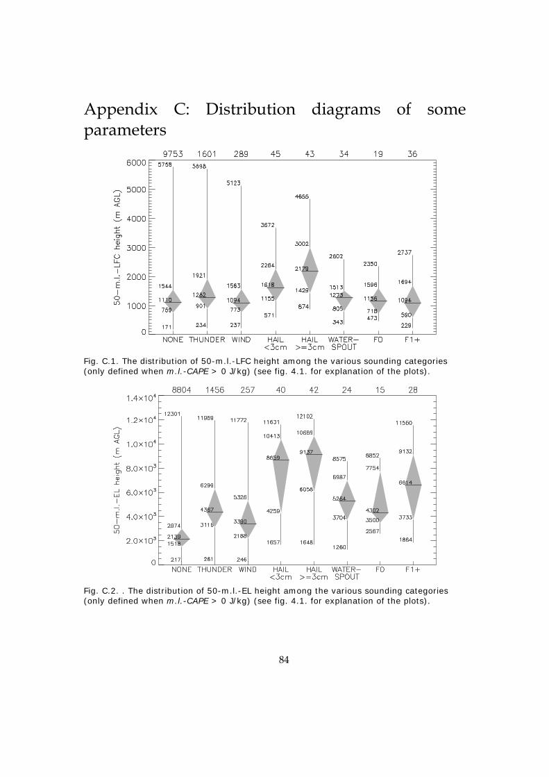
84

Appendix C: Distribution diagrams of some parameters

Fig. C.1. The distribution of 50-m.l.-LFC height among the various sounding categories (only defined when m.l.-CAPE > 0 J/kg) (see fig. 4.1. for explanation of the plots).

Fig. C.2. . The distribution of 50-m.l.-EL height among the various sounding categories (only defined when m.l.-CAPE > 0 J/kg) (see fig. 4.1. for explanation of the plots).

85

Fig. C.3. Fig. C.2. . The distribution of 50-m.l.-CIN among the various sounding categories (only defined when m.l.-CAPE > 0 J/kg) (see fig. 4.1. for explanation of the plots).

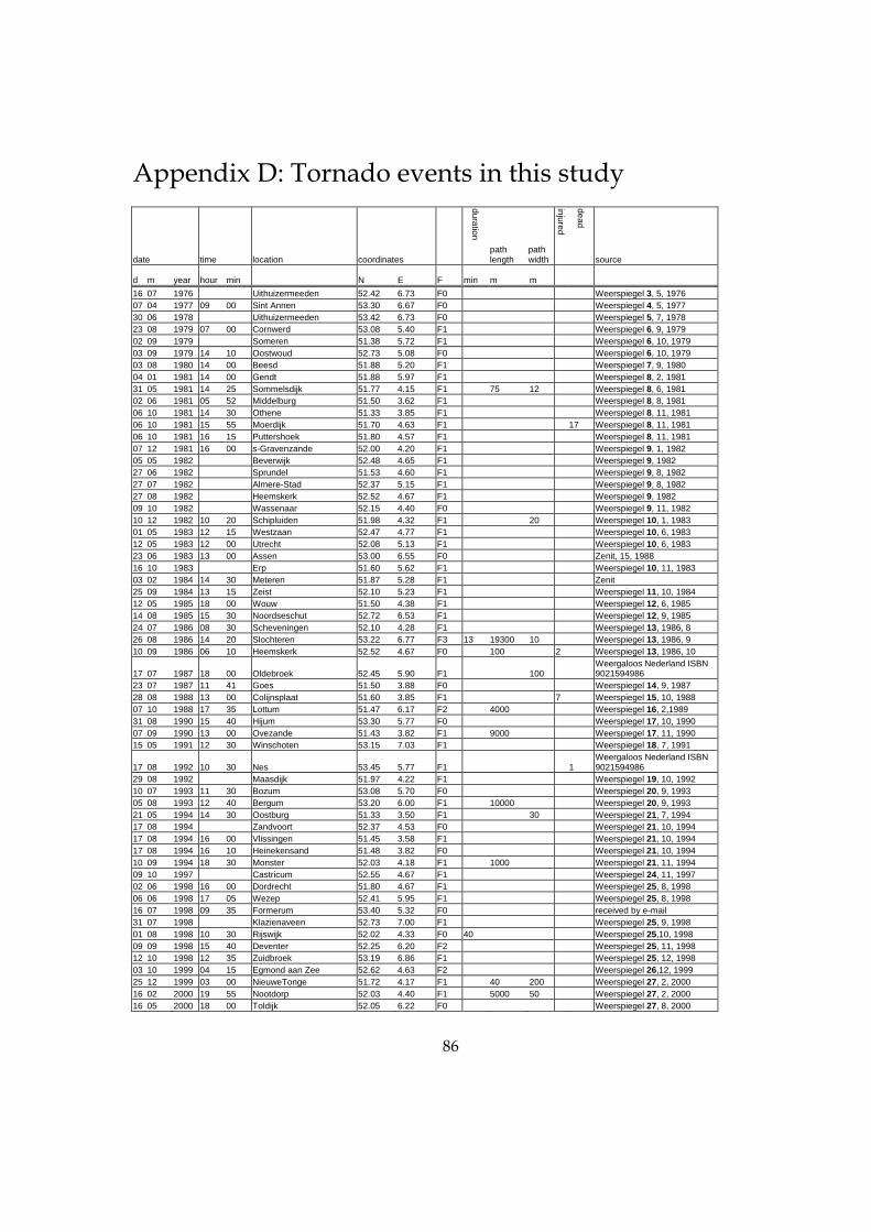
86

Appendix D: Tornado events in this study

date time location coordinates

duration

path length

path width

injured

dead

source

d m year hour min N E F min m m 16 07 1976 Uithuizermeeden 52.42 6.73 F0 Weerspiegel 3, 5, 1976 07 04 1977 09 00 Sint Annen 53.30 6.67 F0 Weerspiegel 4, 5, 1977 30 06 1978 Uithuizermeeden 53.42 6.73 F0 Weerspiegel 5, 7, 1978 23 08 1979 07 00 Cornwerd 53.08 5.40 F1 Weerspiegel 6, 9, 1979 02 09 1979 Someren 51.38 5.72 F1 Weerspiegel 6, 10, 1979 03 09 1979 14 10 Oostwoud 52.73 5.08 F0 Weerspiegel 6, 10, 1979 03 08 1980 14 00 Beesd 51.88 5.20 F1 Weerspiegel 7, 9, 1980 04 01 1981 14 00 Gendt 51.88 5.97 F1 Weerspiegel 8, 2, 1981 31 05 1981 14 25 Sommelsdijk 51.77 4.15 F1 75 12 Weerspiegel 8, 6, 1981 02 06 1981 05 52 Middelburg 51.50 3.62 F1 Weerspiegel 8, 8, 1981 06 10 1981 14 30 Othene 51.33 3.85 F1 Weerspiegel 8, 11, 1981 06 10 1981 15 55 Moerdijk 51.70 4.63 F1 17 Weerspiegel 8, 11, 1981 06 10 1981 16 15 Puttershoek 51.80 4.57 F1 Weerspiegel 8, 11, 1981 07 12 1981 16 00 s-Gravenzande 52.00 4.20 F1 Weerspiegel 9, 1, 1982 05 05 1982 Beverwijk 52.48 4.65 F1 Weerspiegel 9, 1982 27 06 1982 Sprundel 51.53 4.60 F1 Weerspiegel 9, 8, 1982 27 07 1982 Almere-Stad 52.37 5.15 F1 Weerspiegel 9, 8, 1982 27 08 1982 Heemskerk 52.52 4.67 F1 Weerspiegel 9, 1982 09 10 1982 Wassenaar 52.15 4.40 F0 Weerspiegel 9, 11, 1982 10 12 1982 10 20 Schipluiden 51.98 4.32 F1 20 Weerspiegel 10, 1, 1983 01 05 1983 12 15 Westzaan 52.47 4.77 F1 Weerspiegel 10, 6, 1983 12 05 1983 12 00 Utrecht 52.08 5.13 F1 Weerspiegel 10, 6, 1983 23 06 1983 13 00 Assen 53.00 6.55 F0 Zenit, 15, 1988 16 10 1983 Erp 51.60 5.62 F1 Weerspiegel 10, 11, 1983 03 02 1984 14 30 Meteren 51.87 5.28 F1 Zenit 25 09 1984 13 15 Zeist 52.10 5.23 F1 Weerspiegel 11, 10, 1984 12 05 1985 18 00 Wouw 51.50 4.38 F1 Weerspiegel 12, 6, 1985 14 08 1985 15 30 Noordseschut 52.72 6.53 F1 Weerspiegel 12, 9, 1985 24 07 1986 08 30 Scheveningen 52.10 4.28 F1 Weerspiegel 13, 1986, 8 26 08 1986 14 20 Slochteren 53.22 6.77 F3 13 19300 10 Weerspiegel 13, 1986, 9 10 09 1986 06 10 Heemskerk 52.52 4.67 F0 100 2 Weerspiegel 13, 1986, 10

17 07 1987 18 00 Oldebroek 52.45 5.90 F1 100 Weergaloos Nederland ISBN 9021594986

23 07 1987 11 41 Goes 51.50 3.88 F0 Weerspiegel 14, 9, 1987 28 08 1988 13 00 Colijnsplaat 51.60 3.85 F1 7 Weerspiegel 15, 10, 1988 07 10 1988 17 35 Lottum 51.47 6.17 F2 4000 Weerspiegel 16, 2,1989 31 08 1990 15 40 Hijum 53.30 5.77 F0 Weerspiegel 17, 10, 1990 07 09 1990 13 00 Ovezande 51.43 3.82 F1 9000 Weerspiegel 17, 11, 1990 15 05 1991 12 30 Winschoten 53.15 7.03 F1 Weerspiegel 18, 7, 1991

17 08 1992 10 30 Nes 53.45 5.77 F1 1 Weergaloos Nederland ISBN 9021594986

29 08 1992 Maasdijk 51.97 4.22 F1 Weerspiegel 19, 10, 1992 10 07 1993 11 30 Bozum 53.08 5.70 F0 Weerspiegel 20, 9, 1993 05 08 1993 12 40 Bergum 53.20 6.00 F1 10000 Weerspiegel 20, 9, 1993 21 05 1994 14 30 Oostburg 51.33 3.50 F1 30 Weerspiegel 21, 7, 1994 17 08 1994 Zandvoort 52.37 4.53 F0 Weerspiegel 21, 10, 1994 17 08 1994 16 00 Vlissingen 51.45 3.58 F1 Weerspiegel 21, 10, 1994 17 08 1994 16 10 Heinekensand 51.48 3.82 F0 Weerspiegel 21, 10, 1994 10 09 1994 18 30 Monster 52.03 4.18 F1 1000 Weerspiegel 21, 11, 1994 09 10 1997 Castricum 52.55 4.67 F1 Weerspiegel 24, 11, 1997 02 06 1998 16 00 Dordrecht 51.80 4.67 F1 Weerspiegel 25, 8, 1998 06 06 1998 17 05 Wezep 52.41 5.95 F1 Weerspiegel 25, 8, 1998 16 07 1998 09 35 Formerum 53.40 5.32 F0 received by e-mail 31 07 1998 Klazienaveen 52.73 7.00 F1 Weerspiegel 25, 9, 1998 01 08 1998 10 30 Rijswijk 52.02 4.33 F0 40 Weerspiegel 25,10, 1998 09 09 1998 15 40 Deventer 52.25 6.20 F2 Weerspiegel 25, 11, 1998 12 10 1998 12 35 Zuidbroek 53.19 6.86 F1 Weerspiegel 25, 12, 1998 03 10 1999 04 15 Egmond aan Zee 52.62 4.63 F2 Weerspiegel 26,12, 1999 25 12 1999 03 00 NieuweTonge 51.72 4.17 F1 40 200 Weerspiegel 27, 2, 2000 16 02 2000 19 55 Nootdorp 52.03 4.40 F1 5000 50 Weerspiegel 27, 2, 2000 16 05 2000 18 00 Toldijk 52.05 6.22 F0 Weerspiegel 27, 8, 2000

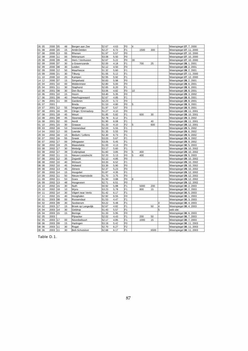
87

26 05 2000 05 48 Bergen aan Zee 52.67 4.63 F0 4 Weerspiegel 27, 7, 2000 01 08 2000 20 15 Ambt-Delden 52.27 6.72 F1 1500 300 Weerspiegel 27, 11, 2000 07 08 2000 13 55 Rhenen 51.97 5.57 F0 Weerspiegel 27, 10, 2000 22 08 2000 11 00 Witmarsum 53.08 5.50 F0 Weerspiegel 27, 10, 2000 29 08 2000 09 40 Hem / Venhuizen 52.67 5.22 F0 30 Weerspiegel 27, 10, 2000 02 09 2000 07 30 s-Gravenzande 52.00 4.18 F1 700 25 Weerspiegel 28, 1, 2001 02 09 2000 08 30 Leiden 52.12 4.50 F0 Weerspiegel 28, 2, 2001 02 09 2000 12 50 Maarheeze 51.32 5.60 F1 Weerspiegel 28, 2, 2001 15 09 2000 21 30 Tilburg 51.55 5.12 F1 Weerspiegel 27, 11, 2000 11 10 2000 10 20 Kampen 52.55 5.92 F1 Weerspiegel 27, 12, 2000 14 12 2000 07 15 Simpelveld 50.83 5.98 F0 Weerspiegel 28, 2, 2001 20 04 2001 10 00 Middenmeer 52.80 5.00 F0 Weerspiegel 28, 6, 2001 25 04 2001 11 30 Staphorst 52.65 6.20 F1 Weerspiegel 28, 6, 2001 10 06 2001 08 30 Den Burg 53.06 4.82 F0 10 Weerspiegel 28, 8, 2001 10 06 2001 10 15 Hoorn 53.40 5.35 F0 Weerspiegel 29, 3, 2002 17 06 2001 09 40 Heerhugowaard 52.67 4.85 F1 Weerspiegel 28, 8, 2001 17 06 2001 11 00 Garderen 52.23 5.72 F0 Weerspiegel 28, 8, 2001 05 07 2001 Breda 51.53 4.80 F0 5 Weerspiegel 28, 9, 2001 19 07 2001 12 55 Wageningen 51.97 5.67 F0 Weerspiegel 28, 9, 2001 07 08 2001 16 00 Clinge / Emmadorp 51.27 4.10 F0 Weerspiegel 28, 11, 2001 07 08 2001 18 45 Weurt 51.85 5.82 F1 600 30 Weerspiegel 28, 10, 2001 10 08 2001 09 45 Steenwijk 52.78 6.12 F1 Weerspiegel 29, 3, 2002 16 08 2001 02 00 Aerdt 51.90 6.08 F1 40 Weerspiegel 28, 11, 2001 01 10 2001 15 30 Graauw 51.33 4.10 F2 5 600 Weerspiegel 28, 12, 2001 09 03 2002 16 53 Veenendaal 52.03 5.55 F1 Weerspiegel 29, 5, 2002 14 04 2002 12 00 Leende 51.35 5.55 F0 Weerspiegel 29, 6, 2002 29 04 2002 16 15 Bedum / Lellens 52.30 6.73 F1 Weerspiegel 29, 6, 2002 30 07 2002 16 55 Sneek 53.03 5.67 F1 Weerspiegel 29, 9, 2002 30 07 2002 17 00 Allingawier 53.05 5.45 F1 Weerspiegel 29, 9, 2002 02 08 2002 19 25 Maasvlakte 51.93 4.13 F0 Weerspiegel 30, 5, 2003 03 08 2002 17 30 Welsrijp 53.17 5.60 F1 Weerspiegel 29, 10, 2002 03 08 2002 17 39 Colijnsplaat 51.60 3.85 F0 5 400 Weerspiegel 29, 10, 2002 07 08 2002 11 15 Nieuw-Loosdrecht 52.20 5.13 F0 5 400 Weerspiegel 29, 5, 2003 07 08 2002 12 35 Zegveld 52.12 4.85 F0 Weerspiegel 29, 10, 2002 08 08 2002 10 40 Winsum 53.33 6.52 F1 Weerspiegel 29, 10, 2002 08 08 2002 10 45 Holwerd 53.39 5.90 F0 Weerspiegel 29, 10, 2002 09 08 2002 13 45 Almere 52.37 5.23 F0 Weerspiegel 29, 10, 2002 07 09 2002 14 15 Hoogvliet 51.87 4.35 F1 Weerspiegel 29, 12, 2002 10 09 2002 11 50 Nieuw-Haamstede 51.70 3.75 F0 Weerspiegel 29, 12, 2002 11 09 2002 11 53 Goes 51.50 3.88 F0 8 Weerspiegel 29, 12, 2002 26 09 2002 13 48 Hoogeveen 52.71 6.51 F0 Weerspiegel 29, 12, 2002 16 10 2002 15 30 Nuth 50.92 5.88 F1 5000 200 Weerspiegel 30, 2, 2003 25 10 2002 18 10 Wyns 53.23 5.78 F1 800 15 Weerspiegel 30, 2, 2003 04 11 2002 14 30 Vilgert near Venlo 51.42 6.17 F1 Weerspiegel 30, 5, 2003 17 11 2002 15 40 Hooghalen 52.92 6.55 F0 Weerspiegel 30, 1, 2003 30 01 2003 08 00 Roosendaal 51.53 4.47 F1 Weerspiegel 30, 3, 2003 04 02 2003 09 30 Sexbierum 53.22 5.48 F1 4 Weerspiegel 30, 4, 2003 04 02 2003 17 15 Broek op Langedijk 52.67 4.82 F1 50 4 Weerspiegel 30, 4, 2003 26 04 2003 14 30 Geldrop 51.43 5.57 F1 5 web site 26 04 2003 15 15 Beringe 51.33 5.95 F0 Weerspiegel 30, 6, 2003 02 05 2003 Pijnacker 52.02 4.43 F1 200 50 Weerspiegel 30, 7, 2003 02 05 2003 17 00 Noordsebuurt 52.17 4.85 F1 1000 15 Weerspiegel 30, 7, 2003 08 06 2003 09 15 Harlingen 53.18 5.42 F0 Weerspiegel 30, 11, 2003 08 06 2003 11 30 Rogat 52.70 6.27 F2 Weerspiegel 30, 11, 2003 08 06 2003 11 30 Belt-Schutsloot 52.68 6.17 F1 6500 Weerspiegel 30, 11, 2003

Table D.1.