16th Australasian Fluid Mechanics ConferenceCrown Plaza, Gold Coast, Australia2-7 December 2007

Sound emission on bubble coalescence: imaging, acoustic and numerical experiments

R. Manasseh 1, G. Riboux 2, A. Bui 1 and F. Risso 2

1Thermal & Fluid Dynamics, CSIROPO Box 56, Highett, Melbourne, VIC 3190 AUSTRALIA

2Institut de Mecanique des Fluides de ToulouseUMR 5502 CNRS-INP-UPS, Allee Camille Soula, Toulouse 31400, FRANCE

Abstract

Laboratory and numerical experiments are presented on theemission of sound on bubble coalescence. The aim was tobetter understand the fluid-dynamical mechanisms leading tosound emission. Bubbles were formed from a needle. Coor-dinated high-speed video and acoustic measurements demon-strated that the emission of high-amplitude sound coincidedwith the coalescence of a primary bubble with a smaller sec-ondary. A numerical simulation was performed using a com-pressible level-set front-capturing code, in which a compress-ible gas and nearly compressible liquid are modelled by a sin-gle set of the Navier-Stokes equations with a generic equationof state for both phases. In the simulations, the spherical pri-mary and secondary bubbles initially at acoustic equilibriumwere brought into contact. The numerical calculations predictedthe frequency of emitted sound and the bubble coalescence dy-namics very well. The results suggest that the equalization ofLaplace pressures could be the mechanism leading to soundemission.

Introduction

The natural frequency emitted by bubbles oscillating volumetri-cally with small amplitude has been theoretically predicted andexperimentally confirmed for nearly a century [36, 28, 38, 20,25]. For millimetre-sized bubbles, an excellent approximationto the natural frequencyf0 is given by Minnaert’s equation [28],

f0 =12π

√3γP0

ρ.

1R0, (1)

whereγ is the ratio of specific heats of gas inside the bubble,P0is the absolute liquid pressure,ρ is the liquid density andR0 isthe equilibrium bubble radius. However, it is more challengingto explain the mechanism with which bubble sound emissionsare initiated. Thus, unlike the frequency, the amplitude of bub-ble sound emissions is difficult to predict. Passive emission ofsmall-amplitude sound by bubbles is common in many practicalindustrial flows [10, 3, 24] or environmental flows [27, 6, 22].The difficulty in predicting the amplitude is one problem in theinterpretation of the signals from such sources [3, 24], leadingto complex signal-processing approaches [1, 22]. Numericalsimulations of compressible multiphase flows, while advancingin quality [e.g. 31, 11, 23, 4] and offering many insights [33] re-quire careful comparison with matching laboratory experimentsin order to elucidate the actual excitation mechanism.

Longuet-Higgins [19] proposed three general mechanisms bywhich the energy giving an initial acoustic perturbation could beimparted to the bubble: (i) a difference in instantaneous Laplacepressure at the instant the bubble is formed; (ii) the radial inrushof liquid as the pinch-off occurs; and (iii) an excitation of thevolumetric or ‘breathing’ mode of the bubble by nonlinear inter-actions of shape modes [17, 18]. It is likely that some of thesemechanisms might apply in some situations, but not in others[12].

Bubbles can emit sound when they pinched off from a parentbody of gas. In this case, the excitation mechanism may be avariant of (ii): it has been observed [12] that a high-speed liquidjet penetrates the bubble on the breaking of the neck that joinsit to its parent body of gas, and may be responsible for com-pressing the trapped gas [26]. This phenomenon remains toorapid for experimental quantification, although new ultra-highspeed cameras may soon permit pinch-off physics to be studied.Longuet-Higgins [20] also proposed that orifice-formed bubblescould make sound by mechanism (iii).

Bubbles can also emit sound when created by the entrapmentof air from a free surface. This might occur in contexts such asraindrop impact [e.g. 35, 34], a plunging jet [e.g. 9, 5] or wave-breaking [e.g. 27, 16, 6, 22]. At the instant the surface closes,pinching off the bubble, there must be a sudden transition froma cavity at atmospheric pressure to a closed bubble in which thepressure exceeds atmospheric by the Laplace pressure due tosurface tension, plus the hydrostatic pressure that must now besupported. Thus, in this second class of phenomena, mechanism(i) is a possible explanation as well as (ii) and (iii). Pumphrey& Elmore [35] created bubbles from drop impacts in the labo-ratory. The amplitude predicted by the Laplace-pressure theorywas only about 25% of the experimental values, and the trendwith bubble size was not predicted. However, statistical confi-dence is hard to obtain in drop-impact experiments unless par-ticular experimental procedures are adopted [e.g. 15], becausethere is considerable variation from drop to drop owing to thenatural variation in impact conditions.

The present paper reports experiments and numerical simula-tions in which bubbles emit sound on coalescence. These bub-bles are formed by pinch-off from an orifice but create theirloudest sounds on coalescence. Unlike earlier acoustic dropimpact studies, repeatability is excellent. Depending on the airflow rate, zero, one, or several coalescences might occur. Allmechanisms (i), (ii) and (iii) are conceivable in this case.

Experimental Method

The general experimental set-up is shown in Figure 1. The testsection was a glass tank 1,000 mm high with a square cross-section of 150 mm. The tank was filled with filtered tap waterat a temperature between 16 and 17◦C. Air bubbles of 1.6 mmdiameter were injected at 85 mm from the bottom of the tank bya needle with an internal diameter of 0.1 mm and a length of 100mm. The rate of bubble production was controlled by adjustingthe pressure in the tank to which the needle is connected.

A high-speed digital video camera (Photron Ultima APX) wasused to film the bubble detachment from the tip of the nee-dle at a frame rate of 20,000 Hz and with an exposure time of1/87,600 s. The region imaged was 1.113 mm high and 2.226mm wide with a resolution 128×256 pixels. Images of the bub-bles were processed to extract their equivalent spherical radiusand location as a function of time [7] .

167

(a)

(b)

Figure 1: Schematic of the experimental set-up. (a) Tank andair supply. (b) Bubble formation and hydrophone.

A Bruel & Kjaer type 8103 hydrophone was used to transducethe acoustic signal. In the relevant 1-10 kHz band, this hy-drophone type has an essentially spherical directivity field, en-suring sounds from any direction are equally transduced, andthere is a linear conversion from transduced voltage to pressurebased on the hydrophone’s individual calibration. The locationof the hydrophone relative to the needle was measured with anaccuracy of±0.1 mm by taking images in two orthogonal direc-tions. Distances were calculated from the true acoustic centreof the 9.5 mm diameter hydrophone. In the present experimentsthe distance from the acoustic centre to the bubble centre was19.1± 0.1 mm. The hydrophone’s presence caused no distur-bance to the bubble formation and rise dynamics.

In a series of initial tests, the hydrophone was traversed in thehorizontal and vertical. This was to check that the sound fieldfell off approximately as 1/r, wherer is the distance from thebubble centre, rather than being significantly affected by soundwave modes or reverberations. Tests were also carried out inlarger tanks to confirm that the 150 mm cross-section of theactual tank did not cause any distortion or modification to theacoustic signal created by bubbles formed from the needle. It

is known that as the tank in which bubbles are formed is madesmaller, there will eventually be an effect on the acoustic signal[30], although this problem is most marked with tanks of circu-lar rather than square cross-section. For the bubbles created inthe present experiments, the tank used was confirmed to be anappropriate size and shape to preclude wall or tank-size effects.

The hydrophone signal was pre-amplified by a Bruel & Kjaertype 2635 charge amplifier set to the individual calibration ofthe hydrophone. The signal was then fed through a purpose-built high-pass 5-pole Bessel filter with a 500 Hz cut-off andan amplitude gain of 10. The high-pass filtering eliminatedany low-frequency pressure fluctuations due to bubble motionwhile preserving completely the bubble-acoustic signals whichwere all above 3 kHz. The filtered signal was digitized by aNational Instruments Data Acquisition Card type 6024E usinghigh-speed data logging software built on the National Instru-ments LabView platform. Considering the typical level of back-ground noise, the random error in transduction of the acousticpressure was less than 10%. This could be improved if neces-sary with low-pass filtering, but for the present paper this accu-racy was sufficient.

The gate signal from the camera was logged on one channelof the datalogging card and the high-pass filtered acoustic sig-nal was logged on a second channel. A nominal logging rateof 120 kHz was used for both channels. However, since a pre-cise comparison of the video and acoustic signals was required,it was noted that no card will in fact digitize data at exactlythe requested rate but at a marginally different rate dependenton the card’s internal arithmetic; in the present experimentsthis marginal difference is sufficient to cause a noticeable mis-alignment of acoustic and video records for the lowest bubble-production rates. The actual logging rate was extracted fromlow-level routines and was found to be 119,760.48 Hz; its useensured a comprehensively precise comparison of acoustic andvideo records.

A digital oscilloscope (Tektronics TDS210) enabled a measure-ment of the rate of production of primary bubbles, by measuringthe interval between pulses. Typically, this could be done withan accuracy of±0.1 s−1 or less; however, as noted below, forthe highest bubble production rates the bubble formation be-came less regular, giving a bubble-production rate estimationaccuracy of±0.5 s−1.

The acoustic pressures measured at the hydrophone were con-verted to the acoustic pressures that would be present at themonitoring point P1 in the numerical simulation (Figure 5), as-suming the acoustic field was monopolar. This can be justifiedby the initial checks that showed the sound pressure amplitudetrending approximately as 1/r with distance.

Acoustic time series and photo-montages of the high-speedvideo frames were generated over the same time window sothat acoustic and visual events could be clearly correlated. Theoriginal size of the frames, which can be seen in Fig. 3, was 128pixels wide by 256 pixels high. Given the desired time windowand the number of frames available within that time, the widthwas calculated of a vertical ‘strip’ of the centre of each frame.For example, to fit 100 frames into a montaged image 400 pixelswide, a vertical strip with the central 4 pixels of each 128 pixelimage was inserted into the montaged image at its correspond-ing time. Since most of the interesting variations occur on thecentreline of the bubble image, this technique preserved muchof the relevant information content of the high-speed video. Inthe extreme, a montage of strips each only 1 pixel wide wouldbe a ‘time-space diagram’ [e.g. 8] showing the rate at whichevents move along the centreline.

168

Numerical methods

The numerical model was based on: i) the level-set method totrack the interfaces; and (ii) an explicit flow solver for com-pressible and nearly incompressible multiphase flows. The gasand liquid are treated as a single continuum fluid with propertiesvarying continuously from gas to liquid states. Coupled witha high-resolution advection scheme, this modelling approachwould allow the description of the movement of gas and fluidand the deformation of the interface separating them on a fixedcomputational mesh [4].

The compressible-nearly incompressible flow solver was basedon the solution of an additional differential equation for pres-sure which was derived from the laws of mass and energy con-servation,

∂p∂t

+~u∇p =−ρc2∇~u, (2)

wherec is the sound speed defined as

c2 = γ(

p+ p∞ρ

),

wherep∞ is a stiffness parameter which is zero for the gas.

A generic equation of state of the form

ρe=p+ γp∞

γ−1, (3)

was used, wheree is the internal energy. The parameterγ hasthe usual meaning of the ratio of specific heats for the gas, butis used in conjunction withp∞ to define the compressibility ofthe liquid.

To track the evolution of the interface, an equation was em-ployed that describes the convection of a level function. Thisfunction is chosen as a signed distance function with the zerolevel set defining the interface location [32], and has the form

φt +(~u·∇)φ = 0. (4)

Using the level function, the steep changes of fluid propertiesacross the interface were smoothed out to minimize numeri-cal oscillations in the solution of Navier-Stokes equations. Thelevel function was also used to calculate interfacial geometri-cal properties, such as the normal vector,~n, and the interfacialcurvature,κ, as follows:

~n =∇φ|∇φ|

, κ = ∇ ·~n,

which in turn define the surface tension.

The system of differential equations describing the fluid and in-terface motions was solved using a projection method. Thiscomprised a prediction and a correction steps (see [40]).The high-resolution numerical schemes ENO (Essentially-Non-Oscillatory) or WENO (Weighted ENO) was used for the con-vective flux calculation.

Experimental Results

At very low bubble production ratesfb less than 3.5 s−1, a se-ries of single bubbles was formed. High-speed imaging con-firmed that there was no coalescence. A very faint signal wasdetectable on amplification of the hydrophone signal, barelyabove the background noise, corresponding to the pinch-off ofeach bubble. In passive-acoustic pinch-off experiments reportedearlier [24, 23], the pinch-off process generated sounds audibleto the naked ear. The bubbles of the present experiment are

approximately 1.6 mm in diameter, whereas bubbles producedin passive-acoustic pinch-off experiments reported earlier [24]ranged from about 4 to 8 mm in diameter. Hence the presentbubbles were one to two orders of magnitude smaller in vol-ume, and thus had much less energy stored on compression andavailable for acoustic emission.

Once the air flow rate is increased such that the bubbling ratefb is above 3.6± 0.1 s−1, occasional loud clicks are audi-ble and corresponding sharp spikes appear on an oscilloscopetrace. These spikes have an order of magnitude greater ampli-tude than the sound created on pinch-off. The frequency was4.15±0.5 kHz which is the Minnaert frequency for a bubble of1.6 mm diameter. Above an air flow rate of 3.8±0.1 s−1, loudclicks are produced regularly and the spikes are spaced regularlyat the bubble production rate. The 3.8±0.1 s−1 threshold forthis phenomenon was quite repeatable in separate experimentsperformed over several different days.

Figure 2: Timeseries of acoustic data over a time of 300 ms,with pressures transformed to values expected at the numericalsimulation monitoring point P1 (see Figure 5). Bubble produc-tion rate 3.82± 0.03 s−1. Series triggered on a pulse at timet = 0.

The acoustic record over a time window of 300 ms is shownin Fig. 2. Acoustic pressures shown have been transformed as-suming a 1/r dependence to the pressures expected at the nu-merical simulation monitoring point P1. Bubbles were formedfrom the needle at 3.8 s−1, which is about 260 ms apart. Theacoustic emissions were a series of sound pulses, an order ofmagnitude amplitude higher than the background. Each pulsewas audible as a single ‘tap’ or ‘knock’ like an individual mu-sical note being struck. These emissions were thus just likeany individual bubble-acoustic pulse reported in the literature[e.g. 28, 39, 14, 24]. Close observation of the high-speed video(Fig. 3) shows that a smaller secondary bubble formed imme-diately after the primary has detached, and soon thereafter co-alesced with it. The details of this phenomenon including thesize of the bubbles had excellent repeatability. The secondarybubble was much smaller, about a sixth the diameter of the pri-mary. It coalesced with the primary before it had detached it-self, thus temporarily re-attaching the primary to the air supply.About 0.1 ms later, it detached itself and was absorbed into theprimary. Loud sound emission under circumstances of bubblecoalescence has been noted before [13].

The circumstances leading to in-line pairing and subsequent co-alescence of orifice-formed bubbles have been studied before,particularly in the chemical engineering literature [29, 2, 37,21]. However, most detailed coalescence studies are for thepairing and coalescence of equal-sized bubbles.

Thus, each of the “3.8 bubbles per second” is really a pri-mary that has coalesced with a secondary immediately follow-

169

first detachmentprimary bubbleformation of

secondary bubbleformation of

final bubblesecondary detachmentt=0 mst=!0.15 ms t=0.05 ms t=0.10 ms t=2.05 ms

t=!3.04 ms t=!1.05 mst=!3.95 mst=!15.15 mst=!0.244 s

sound emissioncoalescence and

Figure 3: Bubble formation sequence. Bubble production ratefb is 3.8 s−1, bubble diameter 1.6 mm, as in Figure 2.

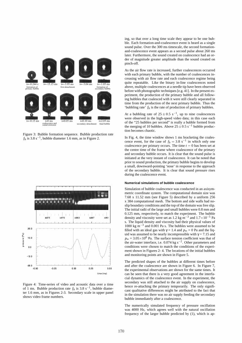
Figure 4: Time-series of video and acoustic data over a timeof 1 ms. Bubble production ratefb is 3.8 s−1, bubble diame-ter 1.6 mm, as in Figures 2-3. Secondary scale in upper panelshows video frame numbers.

ing, so that over a long time scale they appear to be one bub-ble. Each formation-and-coalescence event is heard as a singlesound pulse. Over the 300 ms timescale, the second formation-and-coalescence event appears as a second pulse about 260 mslater. Furthermore, the sound created on coalescence had an or-der of magnitude greater amplitude than the sound created onpinch-off.

As the air flow rate is increased, further coalescences occurredwith each primary bubble, with the number of coalescences in-creasing with air flow rate and each coalescence regime beingquite repeatable. Like the binary in-line coalescences notedabove, multiple coalescences at a needle tip have been observedbefore with photographic techniques [e.g. 41]. In the present ex-periment, the production of the primary bubble and all follow-ing bubbles that coalesced with it were still clearly separated intime from the production of the next primary bubble. Thus the‘bubbling rate’ fb is the rate of production of primary bubbles.

At a bubbling rate of 25± 0.5 s−1, up to nine coalescenceswere observed in the high-speed video data; in this case eachof the “25 bubbles per second” is really a bubble formed fromthe merging of 10 bubbles. Above 25±0.5 s−1 bubble produc-tion becomes chaotic.

In Fig. 4, the time window shows 1 ms bracketing the coales-cence event, for the case offb = 3.8 s−1 in which only onecoalescence per primary occurs. The timet = 0 has been set atthe centre time of the frame where coalescence of the primaryand secondary bubble occurs. It is clear that the sound pulse isinitiated at the very instant of coalescence. It can be noted thatprior to sound production, the primary bubble begins to developa small, downward-pointing ‘nose’ in response to the approachof the secondary bubble. It is clear that sound pressure risesduring the coalescence event.

Numerical simulations of bubble coalescence

Simulation of bubble coalescence was conducted in an axisym-metric coordinate system. The computational domain size was7.68 x 11.52 mm (see Figure 5) described by a uniform 256x 384 computational mesh. The bottom and side walls had no-slip boundary conditions and the top of the domain was free slip.The initial radii of the large and small bubbles were 0.8 mm and0.125 mm, respectively, to match the experiment. The bubbledensity and viscosity were set as 1.2 kg m−3 and 1.7×10−5 Pas. The liquid density and viscosity had their physical values of1000 kg m−3 and 0.001 Pa s. The bubbles were assumed to befilled with an ideal gas withγ = 1.4 andp∞ = 0 Pa and the liq-uid was assumed to be nearly incompressible withγ = 7.15 andp∞ = 3.05×108 Pa. The surface tension coefficient was that ofthe air-water interface, i.e. 0.074 kg s−2. Other parameters andconditions were chosen to match the conditions of the experi-ment shown in Figures 2- 4. The locations of the initial bubblesand monitoring points are shown in Figure 5.

The predicted shapes of the bubbles at different times beforeand after the coalescence are shown in Figure 6. In Figure 7,the experimental observations are shown for the same times. Itcan be seen that there is a very good agreement in the interfa-cial dynamics of the coalescence event. In the experiment, thesecondary was still attached to the air supply on coalescence,hence re-attaching the primary temporarily. The only signifi-cant qualitative differences might be attributed to the fact thatin the simulation there was no air supply feeding the secondarybubble immediately after a coalescence.

The numerically simulated frequency of pressure oscillationwas 4000 Hz, which agrees well with the natural oscillationfrequency of the larger bubble predicted by (1), which is ap-

170

Figure 5: Computational domain with initial bubbles and mon-itoring points P1 and P2.

proximately 4077 Hz. Furthermore, the numerically simulatedfrequency is within about 5% of the experimentally measuredfrequency of about 4150 Hz. The peak pressure at point P1is about 13 Pa, whereas the experimental data, transformed topoint P1, corresponds to about 20 Pa.

Conclusions

A system in which bubbles coalesced on formation generatedloud bubble-acoustic emissions at the instant of coalescence ofsecondary bubbles with the primary bubble. A compressible-flow numerical model based on the level-set method was able to

t = -0.15 t = -0.1 t = -0.05

t = 0. t = 0.05 t = 0.1

Figure 6: Numerical simulation of the bubble coalescence. Unitfor the relative time is ms.

accurately predict both the kinematics of the bubble coalescenceevent and the frequency of the sound emission. The simulationcorrectly predicted the sound pressure amplitude rising at theinstand of coalescence. The numerical model also obtained anestimate of the sound amplitude in the same order as the exper-iment.

The numerical domain was over an order of magnitude smallerthan the experimental domain and so one would not expect thetime series of pressure oscillations to be the same. Nonetheless,the acoustic oscillation frequency of the bubble was predictedto within 5%. The amplitude was less well predicted, being afactor of 1.5-2.0 lower than what would be expected from theexperimental data.

The amplitude of the emitted sound was up to an order of mag-nitude greater than the sound created on pinch-off of the pri-mary bubble. The sound frequency was at the Minnaert fre-quency of the large bubble. As the air flow rate increased, thesize and number of secondary bubbles increased, and the soundamplitude also increased. On coalescence, the sound pressurewas found to always rise initially.

The experiments and the numerical simulations agreed that inthe present coalescence phenomenon there was no jet penetrat-ing the bubble, as found in experiments on sound generationon pinch-off [12, 26]. Hence, mechanism (ii) seems unlikely.The experiments and the numerical simulations also agreed thatsound was emitted at the very instant of bubble coalescence. Atthe time of sound emission, shape-mode distortions have notyet begun to relax, a process that might generate sound emis-sions by mechanism (iii). Mechanism (i), the Laplace-pressureequalization phenomenon, appears to have survived this roughelimination. However, more detailed numerical experimentsand matching laboratory work would have to be performed totest the Laplace-pressure hypothesis.

Future numerical experiments should attempt to examine theLaplace pressure mechanism (i) versus the shape-mode mech-

t = -0.15 t = -0.1 t = -0.05

t = 0. t = 0.05 t = 0.1

Figure 7: Experimental data for the same times as Figure 6.Unit for the relative time is ms.

171

Figure 8: Variation of the pressure.

anism (iii). Laboratory experiments should be conducted inwhich the size of the secondary bubble could be systematicallyvaried, and in which the added complication of re-attachmentcould be avoided.

Acknowledgments

We are grateful to Sebastien Cazin at IMFT for technical helpwith the instrumentation and John Davy at CSIRO for valuablediscussions.

*

References

[1] Al-Masry, W. A., Ali, E. M. and Aqeel, Y. M., Determina-tion of bubble characteristics in bubble columns using sta-tistical analysis of acoustic sound measurements,Chem.Eng. Res. Design, 83(A10), 2005, 1196–1207.

[2] Bhaga, D. and Weber, M. E., In-line interaction of a pairof bubbles in a viscous liquid,Chem. Eng. Sci., 35, 1980,2467–2474.

[3] Boyd, J. W. R. and Varley, J., The uses of passive mea-surement of acoustic emissions from chemical engineer-ing processes,Chem. Eng. Sci., 56, 2001, 1749–1767.

[4] Bui, A. and Manasseh, R., ACFD study of the bubble de-formation during detachment, Fifth International Confer-ence on CFD in the Process Industries, Melbourne, Aus-tralia, 13–15 December 2006, 2006, Paper 053, Paper 053.

[5] Chanson, H. and Manasseh, R., Air entrainment processesof a circular plunging jet: void-fraction and coustic mea-surements,J. of Fluids Eng., 125(5), 2003, 910–921.

[6] Ding, L. and Farmer, D. M., Observations of breaking sur-face wave statistics,J. Phys. Oceanogr., 24, 1994, 1368–1387.

[7] Ellingsen, K. and Risso, F., On the rise of an ellipsoidalbubble in water: oscillatory paths and liquid-induced ve-locity, J. Fluid Mech., 440, 2001, 235–268.

[8] Goharzadeh, A. and Mutabazi, I., Experimental character-ization of intermittency regimes in the couette-taylor sys-tem,Eur. Phys. J. B, 19, 2001, 157–162.

[9] Hahn, T. R., Berger, T. K. and Buckingham, M. J., Acous-tic resonances in the bubble plume formed by a plungingwater jet,Proc. R. Soc. Lond. A, 459, 2003, 1751–1782.

[10] Hsi, R., Tay, M., Bukur, D., Tatterson, G. B. and Morrison,G., Sound spectra of gas dispersion in an agitated tank,Chem. Eng. J., 31, 1985, 153–161.

[11] Hu, Y. Y. and Khoo, B. C., An interface interactionmethod for compressible multifluids,J. Comput. Phys.,198, 2004, 35–64.

[12] Leighton, T. G.,The Acoustic Bubble, Academic Press,London, 1994.

[13] Leighton, T. G., Fagan, K. J. and Field, J. E., Acoustic andphotographic studies of injected bubbles,Eur. J. Phys., 12,1991, 77–85.

[14] Leighton, T. G. and Walton, A. J., An experimental studyof the sound emitted by gas bubbles in a liquid,Eur. J.Phys., 8, 1987, 98–104.

[15] Liow, J. L., Splash formation by spherical drops,J. FluidMech., 427, 2001, 73–105.

[16] Loewen, M. R. and Melville, W. K., Microwave backscat-ter and acoustic radiation from breaking waves,J. FluidMech., 224, 1991, 601–623.

[17] Longuet-Higgins, M. S., Monopole emission of sound byasymmetric bubble oscillations. part 1. normal modes,J.Fluid Mech., 201, 1989, 525–541.

[18] Longuet-Higgins, M. S., Monopole emission of soundby asymmetric bubble oscillations. part 2. an initial-valueproblem,J. Fluid Mech., 201, 1989, 543–565.

[19] Longuet-Higgins, M. S., An analytic model of sound pro-duction by raindrops,J. Fluid Mech., 214, 1990, 395–410.

[20] Longuet-Higgins, M. S., Kerman, B. R. and Lunde, K.,The release of air bubbles from an underwater nozzle,J.Fluid Mech., 230, 1991, 365–390.

[21] Manasseh, R., Bubble-pairing phenomena in spargingfrom vertical-axis nozzles, 24th Australian & NZ Chem-ical Engineering Conference, Sydney, 30 Sep - 2 Oct,1996, volume 5, 27–32, 27–32.

[22] Manasseh, R., A.Babanin, Forbes, C., Rickards, K.,Bobevski, I. and Ooi, A., Passive acoustic determinationof wave-breaking events and their severity across the spec-trum,J. Atmos. Ocean Tech., 23(4), 2006, 599–618.

[23] Manasseh, R., Bui, A., Sanderkot, J. and Ooi, A., Soundemission processes on bubble detachment, 14th Aus-tralasian Fluid Mechanics Conference, Adelaide Univer-sity, Adelaide, Australia, 10-14 December 2001, 2001.

[24] Manasseh, R., LaFontaine, R. F., Davy, J., Shepherd, I. C.and Zhu, Y., Passive acoustic bubble sizing in sparged sys-tems,Exp. Fluids, 30(6), 2001, 672–682.

[25] Manasseh, R., Nikolovska, A., Ooi, A. and Yoshida, S.,Anisotropy in the sound field generated by a bubble chain,J. Sound Vibration, 278 (4-5), 2004, 807–823.

[26] Manasseh, R., Yoshida, S. and Rudman, M., Bubble for-mation processes and bubble acoustic signals, Third Inter-national Conference on Multiphase Flow, Lyon, France,8-12 June, 1998.

172

[27] Melville, W. K., Loewen, M., Felizardo, F., Jessup, A.and Buckingham, M., Acoustic and microwave signaturesof breaking waves.,Nature, 336, 1988, 54–56.

[28] Minnaert, M., On musical air bubbles and the sound ofrunning water,Phil. Mag., 16, 1933, 235–248.

[29] Nevers, N. D. and Wu, J.-L., Bubble coalescence in vis-cous fluids,Am. Inst. Chem. Eng. J., 17, 1971, 182–186.

[30] Nikolovska, A.,Passive acoustic transmission and soundchannelling along bubbly chains, Department of Mechan-ical and Manufacturing Engineering, University of Mel-boune, Australia, 2005.

[31] Oguz, H. and Prosperetti, A., Numerical calculation oftheunderwater noise of rain,J. Fluid Mech., 228, 1993,417–442.

[32] Osher, S. and Sethian, J., Fronts propagating withcurvature-dependent speed: algorithms based onhamilton-jacobi formulations,J. Comp. Phys., 79, 1988,12–49.

[33] Prosperetti, A. and Oguz, H., The impact of drops on liq-uid surfaces and the underwater noise of rain,Ann. Rev.Fluid Mech., 25, 1993, 577–602.

[34] Pumphrey, H. C. and Crum, L. A., Free oscillations ofnear-surface bubbles as a source of the underwater noiseof rain,J. Acous. Soc. Am., 87, 1990, 142–148.

[35] Pumphrey, H. C. and Elmore, P. A., The entrainment ofbubbles by drop impacts,J. Fluid Mech., 220, 1990, 539–567.

[36] Rayleigh, On the pressure developed in a liquid during thecollapse of a spherical cavity,Phil. Mag., 34, 1917, 94–98.

[37] Stewart, C. W., Bubble interaction in low-viscosity liq-uids,Int. J. Multiphase Flow, 21(6), 1995, 1037–1046.

[38] Strasberg, M., The pulsation frequency of nonsphericalgas bubbles in liquid,J. Acoustical Soc. of America, 25(3),1953, 536–537.

[39] Strasberg, M., Gas bubbles as sources of sound in liquid,J. Acoustical Soc. of America, 28(1), 1956, 20–26.

[40] Yoon, S. and Yabe, T., The unified simulation for incom-pressible and compressible flow by the predictor-correctorscheme based on the cip method,Computer Phys. Com-munications, 119, 1999, 149–158.

[41] Yoshida, S., Manasseh, R. and Kajio, N., The structure ofbubble trajectories under continuous sparging conditions,3rd International Conference on Multiphase Flow, Lyon,France, June 1998, 1998, 426 1–8, 426 1–8.

173