sorr1e aspects of many-body problem - progress of theoretical
TRANSCRIPT

Supplement of the Progress of Theoretical Physics, No. 15, 1960
Sorr1e Aspects of Many-Body Problem
Nobuyuki FUKUDA* and Yasushi W ADA**
*Department of Physics, Tokyo University of Education, Tokyo
**Department of Physics, Tokyo University, Tolcyo
. (Received September 26, 1960)
Introduction
Most of the dynamical systems which are treated in quantum mechanics or in quantum field theory consist of many particles interacting with each other, so it may seem at first sight quite peculiar to treat the many body problem as a special topic. But there are some reasons for this as explained in the following.
The atoms which were the first object to be dealt with in quantum mechanics are now among the typical examples of many body systems, and have been investigated in great detail so far. The shell structure of atoms were explained in the following way. Since the Coulomb forces between the orbital electrons are very weak compared with those due to the nucleus, each electron is supposed to move in a common field, i.e. the nuclear Coulomb field and the average field of the other electrons. This average field is called the Hartree field, and its mathematical formulation the Hartree or the Hartree-Fock approximation. The effects of electron correlation were then treated as a perturbation, and led to a detailed explanation of experiments. Similar situations also occur both in the metal and in the nucleus. In the metal, many valence electrons are moving around in a lattice formed by the core atoms, interacting through the Coulomb forces between them. It is known, however, that the free electron model of Sommerfeld and Bloch1
) in which each electron is supposed to move independently in a periodic field can remarkably well explain a huge amount of experimental facts of the metal. In the theory of nucleus, we have the shell model due to Mayer and Jensen, which, to our great surprise, appeared as late as in 1948.2
) In addition, the optical potential and the spin-orbit force between an incident neutron and the nucleus explain the scattering experiment very nicely.
Along with such single particle aspects of some kinds of many body systems, the effects of essential dynamical correlations have been noticed for a long time. The first is the saturation. property of the nucleus. Nuclear force is pretty well known from scattering and other experiments, and the
Dow
nloaded from https://academ
ic.oup.com/ptps/article-abstract/doi/10.1143/PTPS.15.61/1844820 by guest on 15 April 2019

62 N. Fukuda and Y. Wada
"Serber Force" which acts only in even states of angular momenta and vanishes in odd states is likely to be true.3
) But a simple Hartree-Fock approximation violates the saturation condition, because of a small percentage of its exchange part. Next, the free electron model does never give a cohesive energy of the metal and, moreover, the Hartree-Fock correction leads to a wrong dependence on temperature of the electronic specific heat, i. e. T /log T instead of T at low temperatures.4
) Collective aspects of many-body systems deduced from experiments, such as the plasma oscillation of an electron gas, the energy gap for excitations in superconductors, phonon and roton spectrum for excitations in liquid He4 , and various collective motions in nuclei, are far from single particle pictures of the system. Those facts clearly show the importance of dynamical as well as statistical correlation effects of the respective many-body systems, and are our main concern in the following review articles.
We want to point out here some difficulties which we encounter in dealing with the actual many body systems. First of all, in most cases except for the metal, the potentials acting between two particles are of such singular characters at short distances, i.e. stronger than 1/r, that
their Fourier transforms · are divergent. The hard core in nuclear forces is a typical example. Then the ordinary perturbation theory in which the kinetic energy part is taken as a free Hamiltonian is not applicable, since. the corrections to the energy and the wave function become infinite in each order. The Hartree approximation also gives rise to divergence. We call the dynamical correlations resulting from this strong singularity the
short range correlations. The famous Brueckner theory (1954) 5) was
primarily intended to treat these correlations and has been applied with great success to various many body systems. Since the singular short
range forces act only when the two particles come close to each other, one may treat these two particles separately, the dynamical effects of the other particles being neglected so long as the density of the system is not too
high. This is the essential standpoint of Brueckner and is justified by the exact theory of Huang-Yang-Lee (1957) 61 in the low density limit. The second difficulty we want to point out is the so-called long range correlations
which give rise to the plasma oscillation of an electron gas and the phonon excitation of the liquid helium. In this case, many particles interact with each other at one time through the long range Coulomb forces or thanks 'to the Bose condensation. Higher order terms in the perturbation expansions are again divergent, and we are forced to have recourse to some intricate techniques in order to get over this difficulty. Following the pioneer work of Tomonaga (one-dimensional model, 1950) 7
) and Bohm and Pines (1953) ,8) a great progress has been done by Gell-Mann, Brueckner, Sawada et al. (1957) ,9)-
12) in treating the long range correlation of an
Dow
nloaded from https://academ
ic.oup.com/ptps/article-abstract/doi/10.1143/PTPS.15.61/1844820 by guest on 15 April 2019

Some Aspects of Many-Body Problem 63
electron gas, the method of which was applied to the collective motions of the nucleus by Takagi et al. (1959) .13
) . It is shown that the "bubble terms" in the Fermi sea, i.e. the creations and annihilations of a pair of electron and hole, play an essential role in giving rise to the plasma oscillation. The phonon spectrum of the liquid helium was first explained by Bogoliubov (1947) ,141 who applied the method of canonical transformation mixing linearly the creation and annihilation operators. The particle described by the new operators is called the quasiparticle. Then the Hamiltonian is diagonalized leaving out the scattering terms between quasiparticles. It is interesting to notice that the phonon spectrum thus obtained becomes identical with the plasma frequency if the potential is of the Coulomb type, though the origin of correlations is not the same.
One of the recent most remarkable progresses in the many body problems is the theory of superconductivity due to Bardeen, Cooper and Schrieffer (1957) 15
) and to Bogoliubov (1958) .16) It is known for a long
time that an energy gap for excitation spectra is necessary and sufficient for explaining the physical properties of superconductors. Froehlich (1950) 17
)
noticed that the electron-phonon interaction is responsible for the superconductivity in view of the isotope effect of the critical temperature, and that the Fermi surface will .be drastically changed by the effective interaction between electrons resulting from the electron-phonon interaction. Cooper (1956) 18
) then showed that a pair of electrons near the Fermi surface forms a bound state, however weak the coupling may be, on account of the Pauli principle, so long as this coupling is attractive. Following this, Bardeen et al.15
) took an idealized system in which the attractive interaction acts only between a pair of electrons with opposite momenta and spins, and applied a skillful variational method to derive the superconducting state and the energy gap for excitations. The essential feature of this .method is the Hartree approximation taking into account the peculiar statistics of the assembly of electron pairs. The wave function for this system obeys the Bose statistics in which it is symmetric with respect to the interchange· of momenta and spins of two pairs, but satisfies the exclusion principle, i.e. vanishes if any two of the momenta and spins are identical. Therefore, one may say that they are Bose-Fermions or Fermi-Bosons. It is shown by Wada, Takano and Fukuda (1958) 19
) that the operators representing those particles are expressed in terms of the Pauli spin operators, and that the BCS Hamiltonian of the system is equivalent to that of an interacting spin system in an external magnetic field. There had been some doubts about the energy gap obtained by BCS, since the constant terms with respect to the total number might not properly be treated in their variational method, but their results were confirmed in the strong coupling limit by WTF. We would like to note
Dow
nloaded from https://academ
ic.oup.com/ptps/article-abstract/doi/10.1143/PTPS.15.61/1844820 by guest on 15 April 2019

64 N. Fukuda and Y. Wada
that each term of the perturbation expansion in this case is of the order of 1/ N, and is vanishingly small, but is again divergent. Bogoliubov (1958) / 6
) on the other hand, applied his favorite method of canonical transformation to the BCS Hamiltonian and obtained the same result. He then extended this method so as to treat the electron-phonon interaction directly, thus having succeeded in giving a firm basis to the BCS theory;
Those investigations mentioned above revealed a common fact that the perturbation expansions are always divergent and that the solutions have in fact some kind of singularities, e. g., branch point, logarithmic or essential singularity, at the origin of the coupling constant.
It is, however, possible in some cases to obtain the appropriate solutions by partially summing up particular terms of the perturbation expansions up to infinite order. In order to avoid the divergence which may appear in each order, one will apply the adiabatic process, replace, if necessary, a singular potential by the soft one, and make the adiabatic parameter tend to zero, recovering the original potential, after the summation has been done. One of the typical examples for this is Gell-Mann and Brueckner's calculation of the correlation energy of an electron gas at high density.91
Brueckner's theory of reaction matrix is another one which is exact in the low density limit.51 The BCS theory of superconductivity is an exceptional case where the perturbation theory is completely misleading. As a matter of fact, one can exactly sum up all the terms arising from the BCS Hamiltonian, but encounters the difficulty that the energy becomes complex if the potential is attractive. This is probably because the Fermi surface is drastically changed and so the adiabatic theorem does not hold. In spite of a huge amount of recent investigations and great successes in understanding the characteristic features of the respective dynamical systems, we are still pretty far from answering the actual problems in a quantitative way. Even in cases we can get good numerical results, the approximation methods are not well justified since many discarded terms are not properly
estimated. Many problems are solved exactly in the low and high density limit, or in the weak and strong coupling limit, and the future problem is how . to generalize the solutions in these limiting cases so as to treat the actual dynamical systems. One may hope here that the limiting solutions will serve as the zeroth order approximation, so long as they already represent the characteristic correlations of the systems. For instance, the
solutions of an electron gas at high density which include the plasma oscillation and screening effect of the Coulomb interaction will be taken as the starting point in discussing the problem at normal density. Very few investigations have been done along this line, but in· the following articles we will refer to a recent work of Fukuda and Gotos concerning the electron gas.2o)
Dow
nloaded from https://academ
ic.oup.com/ptps/article-abstract/doi/10.1143/PTPS.15.61/1844820 by guest on 15 April 2019

Some Aspects of Many-Body Problem 65
In this article, the structure of perturbation expansions both in timedependent and in time-independent theory is given. The main points are to examine the volume and density dependence of various terms and to eliminate unlinked clusters which otherwise give rise to a terrible divergence. The time-dependent theory is based on the adiabatic theorem whose simple proof was given by Gell-Mann and Low (1951) ,21
) and is expressed in terms of Feynman-Dyson's diagrams. 22
) Unlinked clusters correspond to disconnected "loop" diagrams in this case. The second quantized form is convenient and explained in § 1. For the Fermion system, the Fermi distribution is considered as the vacuum just as in the positron theory. We encounter, however, a difficulty in the Boson system on account of the fact that most of the particles are degenerate in the state of momentum zero. Diagram method is not directly applicable, and unlinked clusters are not simply eliminated. In order that the field theoretic approach may be possible, one has to eliminate the operators referring to momentum zero from the Hamiltonian, which is actually done by Sawada (1959) 23
) and by Hugenholtz and Pines (1959) 24
). In § 2, the ordinary time-dependent and time-independent theories are developed, and their identity is proved by the method of Fukuda and Zemach (1957) .25
) In § 3, the method of Van Hove and Hugenholtz (1957) is explained.26
) The ordinary time-dependent theory is simple in structure, but has a flaw that it is based on the adiabatic theorem not proved in a general way. The time-independent theory, on the other hand, is not based on this theorem, but complicated in structure. The above method lies between these theories and retains both advantages. In § 4, neutral pair theory of scalar meson is discussed which is an example of soluble problems in field theory. It was first considered by Wentzel,27
J who had however, missed an important phenomenon-plasmon. It will be considered from various standpoints in this article. This discussion must be significant as a preparation for the investigation of the theory of electron gas. In §5, the theory of an electron gas by Gell-Mann and Brueckner is given.9
) We have used here a method which employs scattering matrix instead of the auxiliary function introduced by Gell-Mann and Brueckner. In § 6, the theories by Sawada10
) and WentzeP2) are discussed,
which would give the foundation for investigating against the system at intermediate density. The consideration for the anomaly of the specific heat is also presented in this section. Finally in § 7, a new approach to the system of the intermediate density is given. It stands on the expectation that the results of discussions in the low or high density limit may afford a firm basis for further applications once the characteristic difficulties such as short or long range correlations in the system are eliminated.
Dow
nloaded from https://academ
ic.oup.com/ptps/article-abstract/doi/10.1143/PTPS.15.61/1844820 by guest on 15 April 2019

66 N. Fukuda and Y. Wada
§ 1. Formulation of many-body problems
Let us consider an N identical particle system interacting with each
other through a potential V, and put the. total Hamiltonian H as follows:
H=Ho+ V (1•1)
where H 0 is the free Hamiltonian (kinetic energy) which has the following
form for the usual non-relativistic system,
Ho= (1·2)
The unit Pi, 1 is adopted. If one is concerned only with two-body forces,
the potential V is written as
(1•3)
but it may happen that many-body forces will play a role in some cases.
The potential V(n) due .to n-body forces is written as
(1·4)
where v is symmetric with respect to the argument. If the forces origi
nate from field theory as it should be in principle, then the n-body
potential is derived as a result of exchange of (n-1) field particles
(mesons, photons, etc.) between the n particles, which is obviously of
higher orders with respect to the coupling constant. We will restrict
ourselves only to the two-body forces in the following considerations, but
the results can be easily extended to general case.
The state function ?Jf obeys the Schroedinger equation
which is uniquely solved by the initial condition ?Jf(t0)
?Jf(t) = U(t)?Jfo,
U(t) =exp{-iH(t-to)}.
) f
?Jfo as
(1·5)
(1•6)
For the Fermion system ?Jf is anti-symmetric under the interchange of the
coordinates, while for the Boson system it is symmetric, and the symmetric
character is compatible with the Schroedinger equation. In the Heisenberg
representaion, the state function is kept constant, while the operators,
Ail's, describing the system are considered to follow the equation of motion
Dow
nloaded from https://academ
ic.oup.com/ptps/article-abstract/doi/10.1143/PTPS.15.61/1844820 by guest on 15 April 2019

Some Aspects of Afany-Body Problem 67
(1•7)
The operator AH is connected with the operator A in the Schroedinger representation by the unitary transformation, such that
A.F1(t) U- 1(t)AU(t), (1•8)
provided that the both representations are identical at time to. It is very convenient in many cases to formulate the theory according
to the second quantization. Here the field quantity t'(r) and its hermitian conjugate o/*(r) are introduced which are continuous functions of space with components associated with the internal degrees of freedom of the particle. The latter variables may be included in r's. The t' and t'* obey the commutation relations
[ t ( r) , 't ( r') ] ± 0, [ 't ( r) , 't* ( r') ] :±.· a ( r- r') , ( 1• 9)
where the anti-commutator or the commutator appears according as the system is an assembly of Fermion.s or Bosons. Then the density operator p (r) is defined by
p(r) 'o/*(r)'o/(r), (1•10)
which is hermitian and positive definite. The total number operator N is given by
and is easily shown to have eigenvalues, 0, 1, 2, . . . . A complete set of eigenvectors {an} of p(r) are given by
(1·12)
where >o means the "vacuum" state .defined by
(1•13)
Then one can show by making use of the commutation relations (1•9) that
1 V'n {B(r---r1)an-1Cr2, ... , rn)
+eB(r--r2)an-1Cr1, rs, ... , rn)
(1·14)
Dow
nloaded from https://academ
ic.oup.com/ptps/article-abstract/doi/10.1143/PTPS.15.61/1844820 by guest on 15 April 2019

68 N. Fukuda and Y. Wada
where e is equal to 1 for the Fermion and ·+ 1 for the Boson system,
and that 11
p ( r) ltn ( r 1 ' ... ' r n) b a ( r r i) an ( r 1 ' ... ' r n) ' i=l
(1·15)
From (1•15) one sees that an(r1, ... , rn) represents the state of n-particle
system with each particle located at r 1 , r2, · · ·, rn, respectively. Eq. (1•14)
allows us to interpret the operator t'* (r) or t' (r) as creating or annihi
lating a particle at the space point r. Our next task is to express the Hamiltonian in terms of t' and t'*
such that it becomes identical in the coordinate representation with (1•1).
The answer is
Ho 2~ ~d3rf7t'*l7t',
V= ~ ~d3rd3r't'*(r)t'*(r')v(r,r')t(r')t'(r), (1•16)
for the n-body potential, one chooses
vcn) =- !~, r. d3r 1 ... d3r nt'* (rl) ... 'fr* (rn) v (rl' ... 'rn) t (rn) ... + (rl). n. j
(1·17)
As is easily shown, the total number operator N commutes with the total
Hamiltonian H, so is a constant of motion. That is, any state vector in
a subspace spanned by an (with n fixed) for different r's will always
remain within the same subspace though it . changes according to. the
Schroedinger equation. It is sufficient therefore to consider only the sub
space spanned by aN, when one treats an N-particle system. Then the
state vector 'l' is expanded as
'l'= ~?JT(r1, ... , rN)aNCr1, ... , rN)dr1· .. drN, (1·18)
where ?JT(r1 , ... , rN) is a complex function which is shown to be identical
with the state function that we considered in (1• 5). The symmetry
character of this follows from that of aN. Since we have
\d3r(£7t'*Po/)aN(r1, ... , rN) ~L.1iaN(r1, ... , rN),
~ ~d3rd3r'1jr*(r)1r*(r')v(r, r')t'(r')o/(r)aN(rl, ... , rN)
1 2 -tijv(ri, rj)a::NCr1, ... , rN), (1·19)
Dow
nloaded from https://academ
ic.oup.com/ptps/article-abstract/doi/10.1143/PTPS.15.61/1844820 by guest on 15 April 2019

Some Aspects of Many-Body Problem 69
we easily obtain
(1· 20)
where H(r1 , ···, rN) is the same as given in (1•1). By equating the coefficients of aN on both sides of the Schroedinger equation in the abstract Hilbert space, we finally get Eq. (1• 5) which is to be proved.
From Eq. (1•19), one sees that an is an eigenvector for the potential energy with an eigenvalue equal to lts ordinary expression in configuration space. ·This can directly be shown by transforming the potential energy as
V =- ~- ~d3rd3r' p (r) p(r') v (r, r')- --~ Nv (0), (1•21)
with v(O) v(r, r). The second term just cancels the self energy effects (i =j) included in the first term. In order to make the kinetic energy term H 0 diagonal, which is essential for the perturbation theory, one .must introduce the momentum representation as follows. If we expand '1/r(r) in Fourier series as
(1•22)
where Q is the normalization volume, ck and c~ satisfy the commutation relations
(1·23)
The algebraic arguments concerning ,Y.(r) and '1/r*(r) hold true for Ck and C~. The total number operator is expressed by
(1•24)
but C~Ck now means the number of particles with momentum k. Then the kinetic and potential energy are written as
(1·25)
with
V(k k · k k) .}2~\dsrdsr'e-iCk,~k4)r-iCk2-ks)r'v(r, r') 1' 2' 4' 3 "'~ J
which is reduced to
Dow
nloaded from https://academ
ic.oup.com/ptps/article-abstract/doi/10.1143/PTPS.15.61/1844820 by guest on 15 April 2019

70 N. Fukuda and Y. Wada
(1·26)
if v(r, r') is a function of (r-r'), where
(1· 27)
The eigenvectors of nk C~Ck are given by
(1·28)
n
with the eigenvalues 'b O'kk; and H 0 becomes diagonal in this representation. i=l
For the N-particle system it is sufficient as before to consider only the
subspace spanned by ~N·
We would like to note here the equation of motion in the Heisenberg
representation to be satisfied by -t and 'o/'*. Following Eq. (1•7), we have
i-~Y]f~,_t) [H, 'o/'R(r, t)]
fm Ll'o/'z:r(r, t) + ~d3r'pz:r(r't)v(r', r)'t]{(r, t), (1· 29)
which is identical in form to the one-body Schroedinger equation with the
Hamiltonian
H1 = -2~LI+ ~d3r'pz:r(r', t)v(r', r),
PR(r,t) 'ti(r,t)t'H(r,t). (1•30)
The last term expresses the self-interaction which has a natural form for
the system where the sources are distributed continuously. The only
difference is that V'H is not a c-number but an operator satisfying the
commutation relations (1• 9).
Let us now consider a free Fermion assembly contained in a large
box Q. Its ground state is given by such configuration that each state·
with momentum I pI , where kB' is the Fermi momentum defined by
'b 1 N, is occupied by one particle and all the other states are unoc-IPI :o.kF
cupied. The energy eigenvalue Eji' in this state is, according to (1• 25),
equal to
(1•31)
and the eigenvector ~<ol is, according to (1·28), given by
Dow
nloaded from https://academ
ic.oup.com/ptps/article-abstract/doi/10.1143/PTPS.15.61/1844820 by guest on 15 April 2019

Some Aspects of Many-Body Problem 71
(1·32)
In the presence of interaction V, some of the particles under the Fermi surface will jump out and collide with each other again and again, thus the Fermi distribution may be drastically changed. In order to treat such interactions, it is sometimes convenient to perform a canonical transformation in which the role of creation and annihilation of a particle under the Fermi surface is reversed just as in the original theory of positrons. That is, we will put
cp ap , for I pI >kll,
Cp bi, c; bp, for I pI l I (1·33)
and interpret bP and b: as the annihilation and creation operator of a "hole" with momentum p. This canonical transformation necessarily transforms the free ground state (1• 32) into a new "vacuum" defined by
(1·34)
i.e. the state with no particles and no holes. Then we have, for instance,
(1·35)
and the potential V is decomposed into complicated elementary processes. We would like to note that the Feynman-Dyson techniques in field theory can be easily applied to the many body problem only in the present formalism.
Next we will consider a free Boson system. In its ground state, all the particles are degenerate in the state with momentum zero. The total energy is therefore zero and its eigenvector is given by
(1·36)
On account of interactions between the particles, this state may be greatly modified as in the case of Fermi distribution. It is again convenient to adopt a formalism in which the free ground state can be treated as "vacuum". First of all, let us consider a Hilbert space spanned by a set of orthogonal vectors
I Np> = n ~7'! ..... ~··· cc;)NP >o' Cp>o 0, (p=fO)' P'ft0y Np!
b Np<N, P*O
(1·37)
Dow
nloaded from https://academ
ic.oup.com/ptps/article-abstract/doi/10.1143/PTPS.15.61/1844820 by guest on 15 April 2019

72 N. Fukuda and Y. Wada
which has clearly one-to-one correspondence to the Hilbert space describing our system, i. e. spanned by
I No, Np>=~;N~=' (Ct)No 1! v1' cc:)NP>o' V , P cO p,
No+~ Nt> N. (1•38) po;~O
Especially, the "vacuum" state in the former space >o corresponds to the ground state f91P in the latter. Next, we will build up a Hamiltonian in the former space, including no Co, in such a way that all the matrix elements between the corresponding states are identical. To this end, let us separate the terms containing Co from the Hamiltonian as follows:
~~-J~c;cp+ }vCO)CtCtCoCo+v(O)~'C~Cp+ ~'v(q)C:c~cqco
+ ~'v(q)C:c;_qCpCo+h. c.+ ~'v(q)C:c-:CoCo+h. c.
(1·39)
where the prime means that the summation is to be carried out over all momenta attached to C's not equal to zero. We notice that
CtCo N ~ ~~c;cp N ~ ~' Np,
CtCtCoCo (N- ~'Np) (N- ~'Np-1).
Next, one can show making use of Eq. (1 • 14) that
(1·40)
<N~, N~ I c:c;_.qcpco I No, Nq> ,; No-Ol'i~J No-l<Nqr I c:c:-qcp I Nq>,
<N~, N~ I c:c:qCoCo I No' Nq> vNo(No iY ON~ 'No-2<N~ I c:c:q I Nq>, (1·41)
where one may omit the delta symbol owing to No+ ~'Np N. Therefore, our aim can be attained both by Eq. (1 e40) and by the replacement
c:cp_:cpco
c:c-:coCo
c:cp-~Cp (N- ~' Np) 112,
c:C-!(N- ~'Np) 11 2 (N- ~'Np 1) 112• (1·42)
Our effective Hamiltonian is non-linear but is very much simplified in the case where the total number of excited particles ~' NP can be neglected compared to N. Then we have
(1•43)
Dow
nloaded from https://academ
ic.oup.com/ptps/article-abstract/doi/10.1143/PTPS.15.61/1844820 by guest on 15 April 2019

Some Aspects of Many-Body Problem 73
§ 2. Conventional perturbation theory
The time-independent Schroedinger equation for the many-particle system is given by
(Ho+ V)W EW (2•1)
which is reduced, in the absence of interaction, to
(2·2)
We will assume that
lim \ft cp, lim (2·3) v...,.o v...,.o
The normalization conditions of '¥ and <I> are, for the sake of convenience, taken as
(2·4)
Introducing an operator ] and the energy shift JE defined by
JE=E--E0 , (2·5)
one can easily obtain from Eqs. (2 •1) and (2 G 2) a set of equations to determine f and JE as
(E0 H 0)]= V]-JE]
JE=<(vl V]I<P> <VJ>. } (2•6)
If we can expand J and JE in the power series of the coupling constant as
= = ]=b](n), JE=bJE<nl, JE<nl=<VJ<n-ll>, (2·7)
n=O n=l
we get the following recurrence formula, noticing the normalization conditions (2•4):
J<ol=1, (2·8)
where 1 1 p
(2·9)
P being the projection operator to the state <I>. Eqs. (2• 7) and (2•8) are called the time-independent Rayleigh . .Schroedinger perturbation theory.
If we neglect the second term on the right-hand side of Eq. (2·8), the
Dow
nloaded from https://academ
ic.oup.com/ptps/article-abstract/doi/10.1143/PTPS.15.61/1844820 by guest on 15 April 2019

74 N. Fukuda and Y. Wada
n-th order term J<nl has a simple form
](n)~~~ v_l_ ... _1-_ V with n V's. a a a
(2·10)
We will examine, as an illustration, the SJ or N dependence of LJE<n)
< V]<n-1)>· There are two types of contributions, one in which all the
particles (and holes) appearing in the intermediate states interact directly
or indirectly and the other which consists of a product of the first type
contributions. The former is called the linked terms and the latter the
"unlinked terms". The SJ-dependence of a linked term is simply evaluated
by taking into account the momentum conservation at each vertex. V is
inversely proportional to SJ as is seen from (1•26) and the n V's give rise
to a factor 1/ SJn. The number of independent momenta of all the inter
mediate states are equal to n + 1 for the Fermion system on account of
momentum conservation and the sum over them gives a factor SJn+l, thus
any linked term is proportional to Q or N. The result is true also for
the Boson system. This is quite reasonable since the energy per particle
is finite as it should be. However, the unlinked terms lead to higher
powers of SJ which is obviously an absurd result. In order to overcome
this difficulty, one has to show that the contributions arising from the
second term on the right-hand side of Eq. (2·8) actually cancel the
unlinked terms. The direct prqof up to fourth order was given by
Brueckner,28) but is difficult to extend it to the general case. For this
purpose, we had better take recourse either to the time-dependent pertur
bation theory or to the method due to Van Hove and Hugenholtz. Especially,
the latter method shows that in order to get the correct answer one has
only to discard all the unlinked terms appearing in (2 •10), disregarding
the Pauli principle in the intermediate states.
Let us consider the Schroedinger equation in the interaction represen
tation given by
. 8'}t(t) Z---~--
8t v (t) \ff (t)' )
l (2·11)
where a is an adiabatic parameter which is to tend to zero after the
calculation. The transformation function U is defined by
W(t) = U(t, to)'I"(to),
i au~f}_o)_ V(t) U(t, to), U(to, to) 1, (2·12)
and is given in the perturbation theory by
Dow
nloaded from https://academ
ic.oup.com/ptps/article-abstract/doi/10.1143/PTPS.15.61/1844820 by guest on 15 April 2019

Some Aspects of Many-Body Problem 75
U(t, to) (2•13)
The function 'I' satisfying (2•1) and (2·4) is given by
'It lim- U(O, __ c::) <I>-. -aH•O<cf>l U(O, oo) I <I>>'
(2·14)
One can formally extend this adiabatic theorem to any eigenstate other
than the ground state, but the two solutions corresponding to oo may
be different for the excited states. We will show that the denominator in
(2•14) just cancels the contributions from closed loop diagrams or the
unlinked clusters appearing in the numerator. If one decomposes U into normal products, each term consists of an
S product times closed loop contributions. Denoting the S product multi
plied by contractions of the operators which do not involve any closed loop
contributions by the symbol : ...... ; , one has
U(O, oo) 2: Un(O, oo),
Un(O, oo)
(-i)n n n! ~0 =-·-----2J-- . -- dt1 .. ·dtm<TCV(t1)"· V(tm,))>o
n! m=O (m-n) Jm! -oo
X ~~~tm+l"·dtn ; T( V(tm+1) •" V(tn)) :
n
=2:<Un.(O, -oo)>o: Un.-m(O, oo) : . ' (2·15) m=O
from which follows the relation co n
U(O, -oo)=2J 2J<Um(O, -oo)>o: Un-m(O, oo); tz=O m=O
= = 2J<Um(O, oo)>o2J: Un-m(O, -oo) : m=O n=m
<U(O, oo)>o: U(O, oo) : . ' (2•16)
where the expectation value with respect to the ground state of Ho, i.e. <f>0 , is
denoted by < .. · >o. Thus one sees that the unlinked clusters are factorized
in the numerator of (2•14) which are exactly canceled by the denominator.
We will show next that the connected contribution : ; U ( 0, - oo) : is
just equal to J introduced in Eq. (2•5). To this end let us put
U n ( 0, - oo) = u~ , Un(O, -oo): =Un. (2·17)
Then one obtains from (2•13)
(2·18)
Dow
nloaded from https://academ
ic.oup.com/ptps/article-abstract/doi/10.1143/PTPS.15.61/1844820 by guest on 15 April 2019

76 N. Fukuda andY. Wada
and from (2•15) n
U~ "'b<u:r.>un-m , m=O } (2·19)
In order to prove that the Un's satisfy the same equations as (2•8) we first assume that this is true for Uk's up to k<n and then show this is also true for Un. Introducing the identity
1v if"' 1v ··· Um-1 'cJ:' = Um-1 q) + am a
into the equation for Uk , one has
1 Un= Vun-1 an
From Eqs. (2•18) and (2·19), one easily obtains
Un=~ Vu~-1- ~<u:r.>un-rn. an m=l
Substituting (2·19) for u~-1 and making use of
1 1
one has
Now one makes use of
1 Vun-l)· an
(2•20)
(2•21)
(2•22)
(2·23)
(2·24)
(2•25)
in the third term on the right side of (2•24), and Eq. (2•21) in the second term, then one obtains after some rearrangements.
which is further reduced, by substituting (2•25) for <u!m> in the second
Dow
nloaded from https://academ
ic.oup.com/ptps/article-abstract/doi/10.1143/PTPS.15.61/1844820 by guest on 15 April 2019

Some Aspects of Many-Body Problem 77
term and by using (2 • 21) for (1/ an-m) V Un-m-1 in the third term, to
1 n- 2 1 1 Un= Vun-1 + ····, ····-< Vu~-1>··· an zma an--m
n-m-2
b < Vur>Un-m-r-1 r=O
n-1 1 1 { 1 -'b <Vum-1> Un-m+
m=l an an--m
n-m-2
b <Vur>Un-m-r-1+ r=O
With the use of (2•19) and (2•23), one gets
n-m-2
Vu.:n-1> < Vur>Un.-m-r-1
It is easy to show that the third and the fourth terms cancel and one finally has
Un (2•26)
where use has been made of the identity
1 1 +-·-··-·---.. ·- 1 0.
Eq. (2·26) is nothing but Eq. (2•21) for k n, which is to be proved.
We would like to point out here an ambiguity appearing in the calculation of excited states which is connected with the operator 1-P introduced in Eq. (2• 9). This operator is well defined either in the ground state or in the case when the system is enclosed in a finite box, but is not for the infinite medium. As a matter of fact, the above-mentioned proof does hold also for the solution ; U(O, oo) ; which is in general different from : U(O, - oo) : . One must therefore be extremely careful for treating the excited states, and not simply replace 1-P by the principal value. This point was first discussed by Fukuda and Newton in a simple example.29
)
For the ground state, however, one may put a. equal to zero in Eq. (2•18)
Dow
nloaded from https://academ
ic.oup.com/ptps/article-abstract/doi/10.1143/PTPS.15.61/1844820 by guest on 15 April 2019

78 N. Fukuda andY. Wada
since 1/am does not give rise to any ambiguity and obtains a simple expression for U(O, -oo)<P as
U(O, 00 )<P= b ~~- v <P. . = ( 1 )n 11=0 a
(2·27)
One has to take only the linked diagrams in order to derive ; U(O,-oo): <P from this:
'l'= : U(O . ' oo) ; <P=Lb ~-- V <P. ,
00
. ( 1 )n 11=0 a
(2·28)
The version of linked diagrams in the time-independent theory will be given in the next section.
In the actual calculation, we are interested in the average values of various physical quantities, Q's, with respect to; say, the ground state, i.e.
(2·29)
Q is in general a function of "Y' and "/P* containing the same number of them like the kinetic and the potential energy. The two-body density function is defined by
<Wip(r)p(r') p(r)a(r r') IW> ---- -~ ---~ -~~-<w r w>-------~----~------· (2·30)
where the factor is chosen such that the integral over r and r' becomes unity. For the ground state, one may choose 'l' in Eq. (2•29) as follows. For the left 'l', one uses 'l'= U(O,oo)<P and for the right 'l', W= U(O, -oo)<P. Then on account of
U(O, oo) = U*( oo, 0),
one obtains.
where
<<~>I U(oo,O)QU(O, -oo) I<P> -<::<l)TVC oo, 6Y 0 C cC - o;;rl <~> >-
-<<~>I T(QS) I<~>> - <<~>IS I<~>> -
S= U(oo, O) U(O, oo) U(oo, --oo)
(2·31)
(2·32)
(2· 33)
is the S-matrix and T(QS) means that the T product is taken for the product of Q and the integrand of S under the assumption that the time attached to Q is zero. In this expression the time integrals run from - oo
Dow
nloaded from https://academ
ic.oup.com/ptps/article-abstract/doi/10.1143/PTPS.15.61/1844820 by guest on 15 April 2019

Some Aspects of Many-Body Problem 79
to oo which makes the actual calculation very easy. The denominator in
(2•32) just cancels the unlinked clusters, that is, all the diagrams which
are not connected with t"'s or 't*'s in Q, and one may write
(2·34)
For the energy shift, one has from (2•6)
JE=<V: U(O, oo) : >, (2·35)
but one can give another expression in the form of (2· 34). To this end,
one considers the coupling constant as a variable parameter, and notices
the relation
V=gV'. (2•36)
Since E(O) is equal to the free kinetic energy of the system, one gets, on
integrating this equation,
(2•37)
where
Therefore the Feynman-Dyson technique for calculating the S-matrix is
directly applicable. The adiabatic theorem may not hold for the excited states on account
of degeneracy but may hold in some cases, and it might happen that the
two solutions turn out to be identical neglecting the phase. Then one has
JEex= ~:dg-}- «~~rot~!~ , <Wero I VI 'l!ero> -·· <w~roTw-;~> __ _
= ( i)1• \"' ~ n! J_~tl .. ·dtn+l< ci>ex I T(V(tl) .. · V(tn+l)) I ci>ew>a(tn+l)
--- --~_( nPn ~~~tl~·~dtn< cl>ew I T( V(tl) ... V(tn)) I cl>ew>
(2· 39)
The Feynman diagrams appearing in the numerator can be classified into
the following two types.
Dow
nloaded from https://academ
ic.oup.com/ptps/article-abstract/doi/10.1143/PTPS.15.61/1844820 by guest on 15 April 2019

80 N. Fukuda and Y. Wada
A) The yertex tn+l is connected at least with one external line, as in Fig. 1.
B) The vertex tn+1 is in the closed loop, not connected with any of the external lines as in Fig. 2.
.pl Pz
t3
p1 Pz
Fig. 1. An example of the diagrams which belong to type A, in which the vertex t·riJ+l is connected with the external line.
P1 Pz
Fig. 2. An example of the diagrams which belong to type B, in which the vertex f·riJ+t is not connected with the external line.
As is easily shown, the contribution from all the diagrams of type B divided by the denominator is identical with (2• 38) and leads to the energy shift of the ground state L1E0 • On the other hand, the contribution from all the closed loops in the type A is canceled by the same type of contribution in the denominator. Thus one has, as the shift of the excitation energy,
~g 1
L1Eex= dg--F(g), 0 g
where L means that only those diagrams connected with the external lines are to be taken.
As an example of the perturbation theory, we will consider a model proposed by Bardeen, Cooper and Schrieffer in connection with the theory of superconductivity.15
) They considered a system of metal electrons with the Hamiltonian
(2·41)
where the second summation runs over a layer with thickness 2w (w being the average phonon energy) around the Fermi surface and
Dow
nloaded from https://academ
ic.oup.com/ptps/article-abstract/doi/10.1143/PTPS.15.61/1844820 by guest on 15 April 2019

Some Aspects of Many-Body Problem 81
(2·42)
(J)k is the Bloch energy and m specifies the spin. In the hole formalism, (2•41) can be written as
H=Ep-gN(O)(J)+ b (J)knk b (J)knk+ : V:, (2·43) k>kF k:;;kF
where N(O) is the density of states with definite spins at the Fermi surface. (J)k for kP2k>kmin is equal to the Bloch energy minus g, the latter being neglected because g is of the order of Q- 1• We will introduce the interaction representation where the last term of (2•43) is taken as the interaction Hamiltonian. Then one has
: V: -- : V(t) : : ¢>*(t)rj>(t) . ' where
This interaction has a particular form such that a pair of particles, ( k, ~ ) and (k, t ) , always behave as a unit and, once excited, will never be broken up. A typical diagram of a pair break-up given in Fig. 3 gives always a contribution of the order of 1/ Q which is to be neglected.
Let us introduce here the propagator of the pair defined by
D(t t') <T(¢>(t) if>* (t')) >o LJ(IL) 1 b······· .. ..
k>kF 2(J)~c- A- ia
The integral (2 • 38) is simply evaluated as
(2•44)
(2·45)
Fig. 3. A typical diagram of a pair break-up in the Bardeen - Cooper - Schrieffer's model. Fourth order.
(2·46)
(2•47)
The corresponding Feynman diagram is given in Fig. 4. Since LJ(A) vanishes with 1/IL2 as ~L--eo, the path for the integration may be closed with a large semi-circle on the upper half plane. Then the first term of the last expression in (2•47) gives gN(O)(J), and the second term is equal to the sum of residues of the integrand on the upper half plane. The poles of
Dow
nloaded from https://academ
ic.oup.com/ptps/article-abstract/doi/10.1143/PTPS.15.61/1844820 by guest on 15 April 2019

82 N. Fukuda and Y. Wada
this integrand are given by the roots Ak of a secular equation
1 gJ(A). (2•48)
It is easy to show that the Ak's are the
excitation energy of a pair. For a>O, the
Ak's for kE:;;:;:~_k';c:_kmin have positive imaginary
parts, while the Ak's for kmax"?:.k>kF have
negative ones, so one finally obtains
£1E'=gN(O)(J)+ b (2(J)k-.1k). (2·49) kF>k
The true energy shift is obtained by adding
this the term -gN(O)(J) in (2•43):
£1E = b (2(J)k- Ak). kF2k
Fig. 4. An example of the
diagrams corresponding to
(2•47) in which pairs are
never broken up. Fourth
order.
(2•50)
It is not difficult to solve the secular equation (2•46) analytically for large
!2, but we do not enter into this here and content ourselves with its
graphical representation in Fig. 5. In the case of the repulsive interaction,
Fig. 5. Function L1 (A.), abscissa of each black point gives the value of each A.k.
In the case of the repulsive interaction g<O all A.k's are real, meanwhile
in the case of the attractive interaction we have always a pair of the
complex A.k in the limit n-Hx>,
all the Ak's are real and (2•50) gives a reasonable result. The Amin, how
ever, has an essential singularity at g=O like exp(1/gN(O)) and the
perturbation expansion is divergent. In the case of the attractive inter
action (g>O) of the BCS theory, Akp and the next root are real only for
a sufficiently small volume Q and in the limit Q--;..oo, one has
2(}) Ak F 2(}) f i ~- .. _.,=c;==:::T:=c=·==··""·'- (2•51)
Dow
nloaded from https://academ
ic.oup.com/ptps/article-abstract/doi/10.1143/PTPS.15.61/1844820 by guest on 15 April 2019

Some Aspects of Many-Body Problem 83
which shows that the adiabatic theorem is not applicable.
§ 3. The method of Van Hove and Hugenholtz
Let us first introduce the transformation function in the Schroedinger representation defined by
U(t) e-tilotU(t, 0), (3•1)
which satisfies
.dU HU z--~~- = dt '
U(O) =1. (3•2)
According to the adiabatic theorem, the eigenstates of the system are determined by lim U(t), but we consider here a related operator, the resol-
t-'J>=
vent R(z), which is a function of a complex variable z defined by
1 R(z) = -·----·······-. H-z (3•3)
There exists a simple relation between U(t) ·and R(z)
(3•4)
where the path of integration is a contour around the real axis of the z plane as shown in Fig. 6. The perturbation expansion of R(z) is given by
We will show in the following that the behavior of our dynamical system can be completely determined by the matrix elements of R(z). We consider here the Fermion system for simplicity, but the method is equally applicable to the Boson system.
(3•5)
real axis
Fig. 6. Path of the integration in the integral in (3•4).
On account of anticommutativity of Ck's the interaction Hamiltonian may be written as
(3·6)
where
Dow
nloaded from https://academ
ic.oup.com/ptps/article-abstract/doi/10.1143/PTPS.15.61/1844820 by guest on 15 April 2019

84 N. Fukuda and Y. Wada
which is always zero for k 3 k4. We do not introduce the creation and
annihilation operators for particles and holes explicitly, but instead distin
guish them by the symbols of momenta, that is, we use k's for momenta
greater than kF) and m's for those smaller than k]i'. Therefore the creation
operators for the particle and the hole are represented by C~ and Cm,
respectively. With this understanding, we consider, as an example, the
second order matrix element
<13IR(2l(z) la>=<m; k3k2jR<2l(z) lk1;>
1 I6t•Pn's(l1121 V 11314) Cn1n2J VI ll3D4)
x(<PoiC;ck3CkzH1- C~CtCbC14H. J ~c:1c:zcn3Cn4H .. ~L.c~li<Po),
0 z 0 z 0 z (3·8)
where a is an one particle state with the momentum k1 and [3 is composed
of two particles k2, k3 and one hole m. The summations are extended over
all momenta, both inside and outside the Fermi surface. In this way,
any matrix element is reduced to the "vacuum" expectation value of a
function of operators, which is different from zero only if one can associate
C~ or Cm on the right side with Ck or C! on the left side. Such an
association may be performed in different ways. Putting, for instance,
l1 k2, 12 k3, 13 n2 k4, 14 n1 k5, n3 m, n4 k1, one has
···1·~6······ ~ Ck2k3l v I k4k5) Ck5k41 v I mk1) k4k5
x(<Po I c; CkaChH. )- C~2C~3Ck4Cks H. )- CIZsC~CmCkcH~_! -· Ck~ I <Po). 0 -Z o-Z o-Z
(3·9)
Any term of Eq. (3•8) can be conveniently represented by a diagram due
to Hugenholtz as follows. 26) The v's in the matrix element correspond to
vertices in the diagram. They occur in the same order from right to left
and the four lines joining in a vertex correspond to the C' s and C*' s in
a vertex in the following way:
{ ck •--E--annihilation operator
c; _ __,_
{ c~ --E--•
creation opera tor Cm __,_.
The diagram corresponding to Eq. (3·9) is shown in Fig. 7. The values
of the denominators can be easily calculated from the diagram. If one
interchanges the role of the two C*'s or C's in the same v, one gets the
identical contribution, hence a factor 4 must be added to each v, which
Dow
nloaded from https://academ
ic.oup.com/ptps/article-abstract/doi/10.1143/PTPS.15.61/1844820 by guest on 15 April 2019

Some Aspects of Many-Body Problem 85
gives 16 in our example. However, in doing so, each pair of equivalent lines, i.e. lines between the same two points and with the same direction, is counted twice, so that a factor 1/2 must be added for such a pair. In our example, the lines k4 and k 5 are equivalent. Thus the contribution of Fig. 7 is equal to
Fig. 7. The second order diagram corresponding to Eq. (3•9).
1 ~ Ck2k3l v I k4k5) (k5k41 v I mk1) ~2--~s( E~,~ 2~ ~-:!~-~~~~=-~)( E~~~-2k~_ + ;£~~~~ z }~E~,~-;~-- ;) .
(3·10)
On account of the momentum conservation at each vertex, Eq. (3•10) has a o-factor ok2+ks-m-k 1 , that is, in any matrix element of R(z) the total momentum is always conserved. For large !2, (3·10) becomes independent of !2 disregarding this o-factor.
We would like to make an important remark about the Pauli principle in the intermediate states. In the summation of (3 •10), the terms with k4 = k 5 should be omitted on account of this principle, but one may include them, since they automatically vanish due to (3·7). This holds quite generally. The errors that one makes if one does not take into account the Pauli principle in the intermediate states with particles or holes of equal momenta and spins are canceled exactly by considering a corresponding diagram which is obtained from the former by interchanging the starting vertices of these two lines. If the two lines have the same momenta, the two give the same magnitude with opposite signs. Thus one may completely disregard the Pauli principle in the intermediate states so long as all kinds of diagrams are taken into account.
Diagrams that can be divided into two or more parts without cutting lines are called "disconnected", and all others "connected". The connected parts constituting a disconnected diagram are the components of the diagram. Diagrams without external lines are called ground state diagrams. All the connected diagrams, as we have seen, give !2-independent contributions with a o-factor, while the contribution of a connected ground state diagram is proportional to !2 for large !2, if one considers the matrix elements of R(EF+z) in order to eliminate the !2-dependence of EF in the denominators. On the other hand, a disconnected diagram containing n ground state components is proportional to !Jn·; so, as a result, all matrix elements of R(EF+z) contain terms with arbitrary high powers of !2. Our next task is to show how this difficulty does not appear in the calculation
Dow
nloaded from https://academ
ic.oup.com/ptps/article-abstract/doi/10.1143/PTPS.15.61/1844820 by guest on 15 April 2019

86 N. Fukuda and Y. Wada
of physical quantities. For this purpose, one first introduces the idea of
convolution which enables one to calculate the matrix element correspond
ing to a diagram from its components. If f(z) and g(z) ·are two functions,
which are regular for non-real z and which vanish like 1/ I z I for I z I ~oo,
one defines the convolution of both functions by
f(z)*g(z) =- _L.-~dCf(z-C)g(t;,). 2nz 'j1
(3•11)
The path of integration is a contour encircling all singular points of the
integrand on the real axis, but not encircling the singular points situated
on the straight line through z parallel to the real axis. It is to be described
counter-clockwise. Under the above conditions, one has by deforming the
contour
f(z)*g(z) g(z)*f(z). (3•12)
Now let us consider two diagrams A and B and denote their contri
butions to R(z) by <a'IA(z) Ia> and <f9'1B(z) !f9>· These two diagrams
can be combined in various ways to form a composite diagram which
contributes to <f9' a' I R(z) I af9>. These composite diagrams only differ by
the order in which the vertices of B occur with respect to the vertices of
A. An example is shown in Fig. 8. Denoting the sum of all these contri
butions by <f9'a'\C(z) \af9>, one can show that
<e'a'IC(EF+z) laf9> <a'\A(EF+z) la>*<f9'\B(EJ)'+z) lf9>. (3·13)
---~---·
a h c
Fig. 8. The three ways in which two diagrams of the first and second order
A and B can be combined to form a diagram of order three.
As an illustration for this proof, one takes the above example and denotes
the energies of the initial, intermediate and final states (compared to E]i')
of B by b1 , b2 and b3 , respectively. Denoting the energies of the initial
and final states of A by a1 and a2, one has
1 1 ·------~-~·············· *--·-----····----··-~
····----·-------
(a1-z)(a2-z) Cb1 z)Cb2--z)Cbs z)
= - --2~{ ~ dt: (a~-= ,f-c a~-=-er· -(-bl-_ z+-t;)(lh _::::?z; + t;)(b-; ··---z···· ·+··-·--:_--:;--·-
Dow
nloaded from https://academ
ic.oup.com/ptps/article-abstract/doi/10.1143/PTPS.15.61/1844820 by guest on 15 April 2019
Some Aspects of Many-Body Problem 87
which, by making use of
is reduced to
Proceeding in the same way, one gets three terms, each with four factors 1/(ai bn-z), which are exactly the products of energy denominators of the three composite diagrams a, b and c of Fig. 8. If we denote the corresponding matrix elements of U(t) of Eq. (3·4) by UA(t), Un(t) and Ua(t) respectively, we have a simple relation
(3·14)
which is familiar in the Feynman diagrams. As we show later on, the energy and the wave function of the ground
state are determined by <a I R(z) I <Po>· Introducing a function D 0 (z) by
(3•15)
one has
(3 ·16)
where the first factor on the right side expresses the contribution from all diagrams without ground state components. If we denote the contribution from all connected ground state diagrams by B0 (z), we easily obtain
1 1 Do(Ell+z) =- z +Bo(z) + 2 Bo(Z)*Bo(z)
+-frBo(Z)*Bo(Z)*Bo(Z) + ···. (3 ·17)
By definition
1 --~·-~---Go (z) z2 ,
(3·18) with
Go(Z) (3·19)
It can be shown in each order term of this expansion that G0 (z) has a
Dow
nloaded from https://academ
ic.oup.com/ptps/article-abstract/doi/10.1143/PTPS.15.61/1844820 by guest on 15 April 2019

88 N. Fukuda and Y. Wada
finite discontinuity at all points x of the positive real axis for SJ~oo, and
that not only G0 (z) but also d/dzGo(z) have well-defined values for z~o.
Putting
(3·20)
one can write
(3·21)
and obtain
1 + __ 0JQ) + -~·-··· _Q_()_(O)_ *_Go_(Ql + .. ·] z z2 2 z2 z2
*--~~2-. 1 + .. ·]. (3 ·22)
The first factor on the right side is simply evaluated to give
_ _l_ + _QoiQ2 _ Qg_(Q): + ... = ___ 1 __ _ z Z 2 z3 z+ G0 (0) ·
(3·23)
If one denotes the second factor by H(z), H(z) has a form
A H(z) =--z--+l(z), (3·24)
where l(z) is finite even at z 0 and
(3·25)
In order to prove (3s24), one makes use of the following lemma: If
/1Cz) and /2(z) are of the form
(3·26)
where a1 , a2 are real, and g 1(z), g 2 (z) are finite even for real z, then
(3·27)
with g(z) being finite for real z. From this lemma one can further
conclude that D0(EP+z) has a pole at z G0 (0) with residue e-c~<ol.
Putting (3•28)
(3 ·29)
Dow
nloaded from https://academ
ic.oup.com/ptps/article-abstract/doi/10.1143/PTPS.15.61/1844820 by guest on 15 April 2019

Some Aspects of Many-Body Problem 89
one sees that the pole of D0 (z) is simply proportional to JJ but the residue, No, exponentially depends on Q. As will be shown next, the energy
shift of the ground state is given by
(3·30)
It is now easy to show that the ground state energy is Eo and the wave function is given by
'Po=C lim(Eo- z)R(z)<I>0 , (3•31) z_,.Eo
where R(z) has a pole at z=Eo since <aiR(EF+z) I<I>o> has a pole at z 0 and D0 (Ez,,+z) at z G0 (0). As a matter of fact, by putting H-Eo H-z+z-E0 , one has
which tends to zero as z_,. Eo. Thus one obtains
(H- Eo)'l!o =0. (3•32)
From the identity
(3•33)
one gets
(3•34)
and, using (3•31) again,
<ct>oi'Vo> c Iim(Eo--z)<<PoiR(z) j<lJo> cNo. z_,.Eo ' (3. 35)
One obtains therefore
lei =No112 for (3·36) and
for (3•37)
If one puts
R(z)<Po =R(z) i!>o*Do (z)
and makes use of the above lemma, one obtains
(3•38)
where the subscript L indicates that only the diagrams without ground
Dow
nloaded from https://academ
ic.oup.com/ptps/article-abstract/doi/10.1143/PTPS.15.61/1844820 by guest on 15 April 2019

90 N. Fukuda and Y. Wada
state components (the so-called linked diagrams) are to be considered. Eq. (3·38) tells us that the probability for finding the free ground state <I>o in the true one is equal to No which is vanishingly small.
Most of the linked diagrams are still disconnected. If one uses the subscript LC for the connected linked diagrams in (3·38), one can show that
(3. 39)
Now we proceed to treat the excited states, in particular the single particle state. For this purpose, let us consider <aiR(z) jk;>, which is written as
1\
b <a"JR(EF+z) Jk;>*<a'JR(EF+z) I<I>o>, rt/rJ,/1 =C't
(3·40) 1\
where <a" I R(z) I k; > is defined as the sum of the contributions of con-nected diagrams only and given by
<a"lR(EF+z) lk;>=<a"i[l----__1~--- V+···] lk;>-~! ___ , H 0 EP Z o Sk Z
(3·41)
where ek k2/2m. If one denotes the diagonal contribution by Dk(z)o(k- k') defined by
Dk(Z)o(k- k')
<;k'j --=-----:=---z-- V-n;·=-kp:- z + ... ] a I k; >' (3·42)
one obtains
-=::::------=1,_--z--- V + · .. ]~ I k; > · Dk C z),
where the prime means that the state I k; > should be excluded from any of intermediate states. The diagrams contributing to Dk (z) may themselves be composed of several diagonal parts as shown in Fig. 9. The total contribution
(3•43)
Fig. 9. A diagram contributing to Dk(z) which is composed of two diagonal parts.
to (3•42) of all irreducible diagonal parts is equal to
Dow
nloaded from https://academ
ic.oup.com/ptps/article-abstract/doi/10.1143/PTPS.15.61/1844820 by guest on 15 April 2019

Some Aspects of Many-Body Problem 91
where
Gk(z)~(k-k') <;k'i[-V+V · 1 . V-·- .. ·]'!k;>, (3•44) Ho-EF-Z a
and one obtains
1 (3·45)
We will now make the assumptions that the function Dk(Z) has a pole (l)k on the real axis with a residue - Nk and that the first factor on the right-hand side of (3•43) has a well-defined value at z (l)k. Then we can show exactly as in the ground state that the wave function of the excited state is given by
'l"k=C lim (Eo (l)k-z)R(z) lk>, (3•46) z->Eo+(t)k
with the eigenvalue Eo+mk with C=N0112Nk. 112• If one expresses the
state Ia> as
Ia> ~cii>o,
one obtains from (3·40)
where
since
Applying the previous lemma to (3•46) and (3•48), one gets 1\
'l"k=Nk112 [ residue of A(EF+z) at (l)k] •No112
X [ residue of R(z) at Eo] <Po ok 'l"o'
where
on account of (3•43).
(3·47)
(3·48)
(3·49)
(3·50)
(3·51)
Let us discuss the assumption that Dk(z) has a pole on the real axis.
Dow
nloaded from https://academ
ic.oup.com/ptps/article-abstract/doi/10.1143/PTPS.15.61/1844820 by guest on 15 April 2019

92 N. Fukuda and Y. Wada
Since R(z) is holomorphic for non-real z, the pole of Dk(z), if any, should
be on the real axis, but Dk(z) has, in general, no poles. From R*(z)
R(z*), one has
(3·52)
Let us write
(3·53)
and look for a root of the equation
(3·54)
In many cases, this has a real solution x =(l)k which is an increasing
function of I k j. The lowest value (l)k for k = kl!' is called the Fermi
energy (l)p. It has been shown that ]k (x) >O for x>kl!' and that ]k (x)
decreases as (x- (l)p) 2 as x tends to (l)p. (l)k is not therefore a pole of
Dk(Z). If x is close to (l)k, one can write
or
where
Dk(x i0)-1 ek-x Kk(x) -i]k(x)
=- i]k ((l)k) + ((l)k- x) (1 + K£((l)k) + if~((l)k)),
Nk.1 = 1 + KU(l)k),
rk : Nk]k C(l)k). 1 f
(3·55)
(3·56)
(3•57)
For x close to (l)p, rk is very small and one may consider as if Dk(z)
has a pole at z=-=(l)k· Under the circumstances, the wave function Wk
derived above represents a metastable state with a lifetime r1;/:
(3·58)
One can also make the same analysis for states with a hole in the
Fermi sea. For m close to kl!', there exists a metastable state with an
approximate energy Eo (l)m, where (l)m can be regarded as the energy of a
particle with momentum rn in the Fermi sea. Thus one may conclude
that a single particle state is well defined for momentum close to kl!'.
In particular, a state with one additional particle at the Fermi sea is
exactly stationary with the energy Eo+(l)Jl·, from which one obtains
Since Q is fixed, one may rewrite this as
Dow
nloaded from https://academ
ic.oup.com/ptps/article-abstract/doi/10.1143/PTPS.15.61/1844820 by guest on 15 April 2019

Some Aspects of Many-Body Problem
{J N Q
93
(3 ·59)
In the case of a Fermi liquid like a nuclear matter, the second term vanishes and one has
(3·60)
As an application of the method of Van Hove and Hugenholtz, we would like to derive the energy of the Fermion and Boson systems in the low density limit. The energy shift of ground state is given by (3•30). For the Fermion system, the momenta ki of the internal particle lines are to be integrated over I ki I >kF, whereas all the hole momenta ffii over I ffii I <kF. If the density p is very small, then kF is also small and each integration over a hole line in this case leads to a factor kij;,, i. e. a factor p. The main contributions in the low density limit come, therefore, from diagrams with the smallest possible number of hole lines. The general diagram of that type is shown in Fig. 10. They exhibit a repeated scattering of two
Fig. 10. A diagram giving the main contribution to the ground state energy in the case of extreme low density.
particle lines and their contribution is proportional to p2t2 = pN. The energy shift per particle is thus proportional to p, while the unperturbed energy is to p213 • We note here that for the system of particles with spin 1/2 one has
(3•61)
(3•62)
From (3•30) one has in this approximation
+ ) b Cm1m2l vI k1k2) Ck2k1l vI m2m1) + .... 4 m1m2 C:m1 C:m2 Sk1 ~ C:k2
(3·63) klk2
Proceeding in a similar manner for Gk(Z) and Gm(z), one finds
Dow
nloaded from https://academ
ic.oup.com/ptps/article-abstract/doi/10.1143/PTPS.15.61/1844820 by guest on 15 April 2019

94 N. Fukuda and Y. Wada
m1
Gm(z)~(m'-m) =:bCmm1lvl m1m')
+ 1 :b .iJ.!l:!!l:~L~ I k1k?) Ck?!:~J~J.!!l:~J11') + .... m1k1k2 Sm1 + 2e:m Sk1 Sk + Z
If one defines a function k(z) by an integral equation
Cl1l2l k(z) 11314) = 01l2l v 11314)
1 :b _Citl_iliJJ k1k21_Ck2k1 I k Cz) 11314) k1k2 Z- Sk1- Sk2
one obtains
The single particle energy is determined by
(JJk = Sk- Kk ((f)k) : Sk- Kk (e:k)'
(3·64)
(3·65)
(3·66)
(3•67)
in the low density limit. For holes, Gm(z) is holomorphic for z= -em,
since the integrand in (3·65) is not singular for Z=em1 +em. Thus one
sees that holes are stationary in this approximation and the energy of a
particle under the Fermi sea has a well-defined meaning for all momenta
m. The energy shift V m for such a particle is equal to Gm (- sm), so one
finds (3•68)
m1
which, together with (3· 66), leads to
(3·69)
The total energy of the system is given by
and one can easily show that the identity (3·59) does actually hold in
the low density limit.
Dow
nloaded from https://academ
ic.oup.com/ptps/article-abstract/doi/10.1143/PTPS.15.61/1844820 by guest on 15 April 2019

Some Aspects of Many-Body Problem 95
In order to examine the structure of k(z), let us first recall the two-particle scattering problem. The Schroedinger equation for the system is (n=1)
(3•70)
which can be separated into equations for the center-of-mass and relative coordinates as
{- --~ L1r+v(r)} ~(r) =--!2
~(r),
1 K 2
--.im---.dRX(R) -- 4mx(R),
where
and
An incident plane wave is represented by
where
k
The T-matrix is defined by
where
(l1l2l T Jlsl4) = <?P'i~i2 1 VI ?P'Isl4> = 0K1K (k' I T I k),
(k'ITik) <~~ilvl~k>,
which leads to an integral equation for T as
Cl1l2l T I lsl4) = CLI21 v 11314) + 1-... ~ (1~12 I v I :l\: 1~2) __ (~~t_L[J}s1_4~- , 2 k1k2 eh eJ4 ek1- ek2
and
(3•71)
(3·72)
(3•73)
(3•74)
(3·75)
(3•76)
(3•77)
(3•78)
(3·79)
(3•80)
Dow
nloaded from https://academ
ic.oup.com/ptps/article-abstract/doi/10.1143/PTPS.15.61/1844820 by guest on 15 April 2019

96 N. Fukuda and Y. Wada
(k' 1 T 1 k) (k' 1 v 1 k) + 1 b _ik' I vJ:t(~) Ck' I T I k) _ k" sk-sktl
(k' I v lk) =v(k- k') +v(k+k').
Comp·arison of (3·80) and (3•65) shows that
(11l2l T I lsl~) (11l2l k (s~s + s1J I lsl4),
(3•81)
(3·82)
if one replaces V by (1 P) V, P being the projection operator into
inside the Fermi sea. One may extend, in the low density limit, the sum over k 1 , k2 in
(3•65) to the momenta smaller than kF in arbitrary ways. One way is a
direct extension and to take the principal value at the poles. Another
extension is to replace v by ( 1 .,,~ 2P) v which amounts to taking into account
the hole-hole scatterings. Finally, one has an extension which is accessible
to a simple physical interpretation but will not be discussed here. In the
low density limit one may put
(3·83)
where a is the scattering length and one obtains from (3 • 66) •
(LlEo)I d it = N(N_=J}c 8rca ow ens y 2 mJJ (3•84)
We would like to note that in the nuclear many-body problem a factor
3/4 x 1/2=3/8 is to be multiplied, which expresses the a priori probability
for two nucleons to approach each other in even orbital states.
Now we turn to the Boson system.30l Taking the effective Hamiltonian
(1• 43), one easily finds that the density dependent contribution comes
from terms including N or N 112 factors. Therefore the main contributions
in the low density limit are obtained by the diagrams shown in Fig. 11,
and one gets
L1Eo= N2 {<OOiviOO>+ ~ ~~2, ~oo~~~~~~<~k~~~~)o> ,, + .. ·}
N2 =-4,-<oo I TIOO>, (3·85)
where the first term corresponds to the second term of (1• 43). <k1k2 ·lvlk3k 4> is defined by (3•7) in which the negative sign of the second
term is changed to positive. From this one obtains
L1E= 2nea eN m '
(3·86)
which is called the Lenz formula.
Dow
nloaded from https://academ
ic.oup.com/ptps/article-abstract/doi/10.1143/PTPS.15.61/1844820 by guest on 15 April 2019

Some Aspects of Many-Body Problem 97
The above approximation has an important advantage that even the singular potential which has no Fourier transform can be treated. One can improve this approximation by replacing v by k(z) in any diagram one considers, thus avoiding the divergence difficulty. Another improvement will be achieved by replacing 1/ (ek z) by Dk(z) and putting
1
Fig. 11. Diagram contributing to L1 Eo in the low density Boson system. The excited particles are indicated by solid lines, and the unexcited particles by broken lines.
(3•87)
Then one has an self-consistant problem to get Wk.
§ 4. Meson pair theory
Let us consider an example of many particle systems which can be exactly solved and enables one to understand the various methods to be applied to the actual many body problem. That is the neutral scalar meson pair theory first discussed by W entzevm The total Hamiltonian of the system is given by
H=Ho+ V,
Ho = --} ~ (n(x) 2 + (17 <P(X)) 2 + tt2<P(X) 2 )d3X,
V= ~ g(~p(x)<P(x)d3x y, ( 4·1)
where <P(x) is the meson field, n(x) its canonical conjugate, tt the meson mass, and p the source function which depends only on r I x j. Expanding <P and n as
<P(X)
n(x)
(4·2) one has
Dow
nloaded from https://academ
ic.oup.com/ptps/article-abstract/doi/10.1143/PTPS.15.61/1844820 by guest on 15 April 2019

98 N. Fukuda and Y. Wada
=- b~-==-~(ak+ak) , V g ( v(k) * )2
2JJ k Y2Wk
v(k) ~p(r)eikxd3x.
In the interaction representation defined by
qJ(X)_,..qJ(X, t) eiHotqJ(x)e-iHot,
the interaction Hamiltonian takes the form
V(t) = ~ '[r(t) 2,
'[r(t) = ~p(r)qJ(X, t)d3x
_-i/ltf ~ ;}~~; -(ake-iw~t + a:eiw~t).
(4•3)
(4•4)
We will first calculate the level shift of the ground state according to
Eqs. (2•37) and (2•38). Substituting (4•4) in (2•38), one obtains
<']to I Vi ']to> <'l'o I ']to::>-
= ( i)ngn+1 roo · .~ 2n+ln! J_~t1·' ·dtn+1L< T( 'fr(t1) 2 • • ·'fr(tn+1) 2) >o8(tn+1).
(4·5)
If one defines the propagator of a meson ·by
one can easily calculate (4•5) following Wick's method, and noticing
(2•37), one has
oo ( _ i)ngn+1 ~oo ilEo b -
2(·-............... -.. _l) dt1· "dln-1-1iJF(tn+1- t1)iJF(t1 t2) "•iJF(ln- tn+1)8(tn+l)
11=o n+ -= •
oo ( _ i)n-1 gn ~""' = b ··· dt1"•dtniJF(t1)iJF(t2) ... JF(tn)8(tl + t2 +'"+in)
11=l 2n -=
=~ ( 2n-lgn\oodJ.(R(A))n= 4i _ _\oodJ.log(l+igR(J.)), (4•7)
11,.1 rcn J-= rc J-= where
(4·8)
The integrand of (4•7) is regular for the complex values of J. different
Dow
nloaded from https://academ
ic.oup.com/ptps/article-abstract/doi/10.1143/PTPS.15.61/1844820 by guest on 15 April 2019

Some Aspects of Many-Body Problem 99
from the zeros of the argument of logarithm satisfying
(4· 9)
Since all these zeros are located just below the positive real axis and just above the negative real axis, and the integrand of (4•7) behaves like 1/ I A 1 2 for I A j-)-oo, one can transform the path into that from - ioo to +ioo, thus obtaining
LIE0 =-I\"" du log[1 + _ _g __ b v2(/{)_;_J. ( 4•10)
4n J_"" tJ k wk+u
We will next calculate the excitation energy according to (2•39). Substitution of (4•4) into F(g) of (2•40) gives for the numerator
~ ( -i) 2gn+l v2(k):_ \'""' dt1···dtn+1B(tn+1)
n =0 Wk~a J- oo
X {LIF(t1- t2)LIF(t2- ts), .. LJF(tn- tn+l) (eiwk<tl-tn+ll +eiwk(tn+1-tll)
1 n-1
+ 2~ ~ LIJi•(tl t2) • .. LJJr(ti- tn+l)L/Ji•(tn+l- ti+l) "•L/JI(tn-1 tn)
X (ei(J)k(tl-tn) +ei(J)k(tn-ttl)} = ~ (- i)ngn+1 v(k) 2
(n + 1)R(wk)n, n=O 2WktJ
and for the denominator
( 4•11)
where T is the time of the whole world. One obtains therefore from (2·40)
There exists a relation between T and tJ as
p(w)Liw p(k)4nk2Lik
T p(w) = 2n-' p(k)
and one can rewrite (4•13) as
(2n) 3 '
Llwk = i- _"!___ log_! _ _ j ~fiC!EiL, __ (j_g k /2n) v_CI!-_2~ kwktJ 1+tgR(wk)
~ tan-c _ _$ t1k --kwktJ 1 + g ak '
(4•13)
(4•14)
(4•15)
Dow
nloaded from https://academ
ic.oup.com/ptps/article-abstract/doi/10.1143/PTPS.15.61/1844820 by guest on 15 April 2019

100 N. Fukuda and Y. Wada
where
( 4•16)
A state with a definite momentum is not an eigenstate of our system, since the total momentum is not conserved, and it is sometimes convenient to expand q; and rc in terms of spherical waves instead of plane waves, containing the system in a large sphere with radius R. Then one sees that only the S-wave meson can interact with the nucleon and the energy shift Limf is given by
( 4•17)
This can also be derived from ( 4·13) by noticing the fact that T is related to R as T = (2mk/ k) R in this case.
We will present an alternative method, the method of normal mode, which has recently been exploited by Bogoliubov for the discussion of phonon excitations and so forth. 14
)'16
) The Hamiltonian ( 4• 3) should be brought into a normal form by a canonical transformation
where
ak-:;..Ak b (akk'ak' + i3kk'a~,), kl
aa* fl/3* 1,
(4•18)
(4·19)
a being the transposed matrix of a. The necessary and sufficient condition for A's being the normal coordinates is given by
(4·20)
where Qk is the energy of the normal mode k. Once the true ground state 'l'0 (Ak'l'o=O) is found, all excited states are obtained by operating a product of A*'s on ':1!0 , e. g. a one-meson state is given by
Substituting (4•3) and (4•18) 1n (4•20), one obtains
with
v(k')
V2wk'
from which a secular equation for Qk is derived:
(4·21)
(4•22)
(4·23)
Dow
nloaded from https://academ
ic.oup.com/ptps/article-abstract/doi/10.1143/PTPS.15.61/1844820 by guest on 15 April 2019

Some Aspects of Many-Body Problem 101
(4•24)
This is identical with Eq. (4•9) by putting A .Qk and a 0. The first · condition of ( 4 •19) determines the constant Nk, which, as is shown by
differentiating ( 4·24) by g, is given by
(4·25)
The energy shift of the ground state should be given by a sum of all the shifts of zero point energies:
(4•26)
which can be written as
(4·27)
where the path is a closed curve which includes all .Qk's and {1),/s but excludes ( = 0. Introducing a function ¢1 ( () defined by
if1 c t:) 1 -~-· ~- ~ ~.~~;- I[ c t: Q~) 1 n c t:- {1)v, (4•28)
one obtains
(4•29)
= -iJ--1!~ ~~ -~ log-~~±~~~~ =_1.~ \oodk~ tan- 1 g{3k •
2n Jo {1)k 1 + g ak (4·29)
It is easy to deform the contour of the first expression of ( 4 • 29) into that of (4•10). If one introduces (4•15) or (4•17) into (4•26) one can directly derive the result ( 4•29). In the former case one has to replace
(4•30)
and in the latter case,
(4•31)
We will next treat the problem by the new Tamm-Dancoff method
Dow
nloaded from https://academ
ic.oup.com/ptps/article-abstract/doi/10.1143/PTPS.15.61/1844820 by guest on 15 April 2019

102 N. Fukuda and Y. Wada
developed by Dyson.31) Let us denote an arbitrary eigenstate by 'I':
(E-H)W=O, (4·32)
Then one can derive
0 <WI (E-H)aki'I'o> (E-Eo)<WiakiWo>+<WI [ak, H] IWo>
= (E-- Eo+ (J)k) <w I ak I 'I' a>+ ~g_'lj_~~}=~ ~~-1!(k')_~-<w I ak' +a~ I W0> s:r.;2(J)k k' JJv2(J)k' '
from which one obtains
Unless the second factor vanishes, one has
Fig .. 12. Function _??"_ ~ v (p L~ .n P oo2-oop2 ,
the abscissa of each black point gives the frequency of each normal mode !J.k • The largest one !J.pl corresponds to the plasmon mode, and the others to the scattering modes.
1 (4·34)
which is identical with (4·24). In this case 'I'' s are automatically restricted to one meson states, since the energy of a many-meson state cannot satisfy ( 4·34). The ·eigenvalues, A= E- E0 , are solved graphically as in Fig. 12. All solutions tend to (J)k as .Q~oo, but if v(k) =0 for k >kmax , there appears another solution .!Jp1 which is greater than (J)max with a finite interval even for .Q~ oo. The former are call~d the scattering solutions and the latter the plasma one. In order to solve the scattering states for .Q~oo, let us put, following Chew, Low and Wick,
(4·35)
Substituting this in (4·29), one obtains
x<~l = -E~+;~! ___ i~-.rl{- ~- ~~~3~'f, v1~~' (ak' +a~,) Jw o.
(4•36)
One has an identity
Dow
nloaded from https://academ
ic.oup.com/ptps/article-abstract/doi/10.1143/PTPS.15.61/1844820 by guest on 15 April 2019

Some Aspects of Many-Body Problem 103
O=akW0 -1 [-~- v(k) :2: y(k') (akr+a~r)]Wo, (4•37)
Eo (J)k -- H JJ ,! 2(J)k k' ,!2(J)k'
which is easily derived from 0 ak(Eo H)W0 • Adding (4•35) and (4•37), one obtains
-qt<~) = (ak+ a~)Wo + [ -;~-+-A=..E~--+ -Jj;~-+ (J)~I ie-1-l]
(4•38)
from which is derived the equation
(4•39)
If one denotes the normalized wave function of the plasma state by W pi
which satisfies
1!~ [ 1 + JJ ~ _:q ~z~_:_ {~~-+~-Eo --.E~+-~~-!-n± i~} Jw pl o,
one obtains
:2:---'l!_(k) (ak+a:)Wo k ,;z(J)k
[ 1 +-~-- ~-v~:~:- {-;~-+iJ- E~- +Eo (J)k 1
H ±ie} J-1
X b:(k')_-qt(~;+CplWpl, (4·40) k' 2(J)k
where
(4•41)
to be calculated later on. If W o is normalized, then
(4•42)
as was proved by Wick, and by noticing (4•40) one obtains
-~~~r~!?- 2~ F, 1 1 ~-~ _!) ~=; :_ ------+ ~ !Cpd 2
Dow
nloaded from https://academ
ic.oup.com/ptps/article-abstract/doi/10.1143/PTPS.15.61/1844820 by guest on 15 April 2019

104 N. Fukuda and Y. Wada
(4·43)
from which one arrives at
LIEo=_!_\gdg/Cpr/ 2 +-~\<>0_dkk tan- 1 -~}~--. 2Q ~o 2n Jo (J)k 1 + g ttk
(4·44)
This is identical with the last expression of ( 4 • 29) except for the first term. It will be shown that if there is a plasma state the transformation of the first expression to the last in ( 4 • 29) is not allowed and that one should treat the finite contributipn from the plasma state separately in ( 4 • 26) . The plasma wave function, 'l' pi , is obtained from ( 4 • 21) by taking Qk as the plasma solution tJp1, i. e.
'l' pi Atr'l' o ,
Ar, = ~ ~~~?-c JJ.,N·~, ak' + ~ .;7~7/,; a;,N_·~,; · a:•,
Np1 = jg /-{~1 -- , (4·45)
and cpl is 'calculated as
=~; Npr=/Q ~il_, (4•46)
where use has been made of (4•23). Thus the first term of (4•44) is rewritten as
(4•47)
as was expected. We will show next that Eq. (4·10) resulting from the perturbation
theory or the first expression of Eq. ( 4 • 29) in Wentzel's theory is also correct, including the plasma contribution. If one defines a complex function f(z) by
(4•48)
from ( 4•43) one obtains
Dow
nloaded from https://academ
ic.oup.com/ptps/article-abstract/doi/10.1143/PTPS.15.61/1844820 by guest on 15 April 2019

Some Aspects of .Many-Body Problem
which is rewritten as
8L1Eo f)g
fJ!Jpl 1 \(J)max /(w + ie) 8g 2n:g·-Im.\.t daJ 1+/(w+ie)
=-L. fJ!Jpr + _ __!_ _ _\ dz __ _j_(z) __ 2 f) g 4n:ig Ja1 1 + f(z) '
on account. of the relation
105
(4·49)
(4·50)
(4·51)
The contour C1 in ( 4·50) is Fig. 13, which can be deformed into C2 , C3 and c4 since the singularity of the integrand of ( 4·50) exists at z Noticing that
_§/I ) Nprl 2 =- g1 :!JgQ! __ , 1 + /(!Jpr) =0, f)z z=Qpl !J u (4·52)
. and that f(z) tends to zero like 1/ I z 12 for I z 1-?oo, one sees that the integral along c4 vanishes and
_1_\ dz f(z) = _ _!__ fJ!Jp1 4n:ig Ja3 1+/(z) 2 f)g '
which cancels the first term of (4•50). After putting z iu, the integral along C 2 leads to
Fig. 13. Paths for the integrations in (4·50.). The integration along C1 is replaced by those along c2' c3 and c4 .
Dow
nloaded from https://academ
ic.oup.com/ptps/article-abstract/doi/10.1143/PTPS.15.61/1844820 by guest on 15 April 2019

106 N. Fukuda and Y. Wada
which is identical with (4•10). Now we will solve the secular equation (4•24). First of all, let us consider
the scattering solution .Qk and put .Qk = Wk + Llwk. Introducing this into
(4•24), and noticing that
(4·53)
one has
(4·54)
where the term (Llwk) 2 in the denominater has been omitted. On account
of WkLIWk kLlk, (4•54) is reduced to
(4•55)
Since the quantities in the bracket become very large at p~k, one may
replace v(p) 2P2 by v(k) 2k2• Noticing
p-k= (n-no) i , and introducing the notation
RLik a=--
one obtains
2:R ~kv(p) 2P2 { k2 ~p2 - k2 -P2~2kL1k} 1 1
Then ( 4 • 55) can be transformed into
1+gak g{3k cotna=O,
from which one has
(4·56)
(4·57)
(4·59)
Dow
nloaded from https://academ
ic.oup.com/ptps/article-abstract/doi/10.1143/PTPS.15.61/1844820 by guest on 15 April 2019

Some Aspects of Many-Body Problem 107
(4·60)
This is identical with (4•17) as it should be. If one adopts the energy shift with a definite momentum, one would obtain the result (4•15).
In order to express tJp1 in terms of f ( z), let us consider the scattering matrix. The S-matrix is defined by
(4·61)
from which the T-matrix is derived as
(4•62)
From (4•38), (4•42) and (4•40) one easily obtains
(k'l T lk) =<W~-; 1 j ;(k) ~-~~!>_2 (ap+a~) IWo> Q 2(l)k p v 2(l)p
. v(k') v(k) ___ {1+f((l)k' ie)}-1. (4•63) Q v2(l)k' -.12(l)k
If one introduces (4•35) in the first expression of (4•63) and makes use of (4•37), one has the Chew-Low-Wick equation:
x v(k) ~ v(p) Q -.12(1);·· p -.12(l)p
<Wol Q ;~~~=-~~~~::--(ap a;) v(k) v(k')
t2 -:;?2;-~-"-· V2;~~
X g v(k') v(p) · * -ti V2~;~--~v2(l);c.·(ap+ap) I Wo>
= __g_ v Ck )_ _ _ES}') + _s:: . v Ck)~- _!!__(!{) __ __ ~!!PJ_ _8tJpl Q v2(l)k- v2(l)k 1 Q -.12m -.12~~-;- (l)Jf'- Q~l a g
(k" I T I k) * (k" I T I k') :. (k" I T I k') * (k" I T I k') - ~ --------------~------------+ b --------------------~. -- -··- . ( 4. 64) k" (l)k 1 + (l)k" k" (l)k1 - aJk" + Ze
Here the second term in the last expression is the contribution from the intermediate plasma state. The contributions from many-meson intermediate states vanish on account of the equation just above (4·34); the
Dow
nloaded from https://academ
ic.oup.com/ptps/article-abstract/doi/10.1143/PTPS.15.61/1844820 by guest on 15 April 2019

108 N. Fukuda andY. Wada
meson production does not occur in the meson pair theory. On account
of (4•63), the T-matrix off the energy shell is related to that on the energy shell as
(k" I T I k') = __El~)~- I~(J)k" (k" I T I k')s v(k ) V (J)k'
(k" I T I k')s= ( k"l T I k' J1-~; 1 1._ ), ) (4•65)
and (4•64) can be transformed to
(k' I T/k)s= SJ _1!.~:~~~+ SJ _!!_~:~2
---;;;~!-!Jf; ~i~ ~ ~~~f~;~~;
(4·66)
Introducing ( 4• 63) into this, multiplying 2(J)k/ g and summing over k, one
has an explicit expression for 8SJ~~J8g which, upon integrating with respect
to g, leads to
SJ~1 =(J)~ax + 2~3- ~:dg ~~ dk 11 +~C~~l2
z~)j2 {2Ref((J)k+ie) + if((J)k+ie) /2},
(4·67)
where use has been made of the secular equation (4·24). We will next obtain the scattering phase shifts. According to Lippman
and Schwinger,32) the eigenvalues of the T-matrix are given by
(4·68)
which shows, as already noticed, that the S-wave can only scatter. From
( 4 • 68) one obtains the phase shift (]s ( k) as
tan(]s(k) = ~Too(P) 1-zrcToo(P)
(4•69)
Comparing this with ( 4·17) one has the following important relation
between the phase shift and the energy shift:
or
1 k -----B(k), R (J)k
1 L1k=-=·-7l(J(k).
(4·70)
Dow
nloaded from https://academ
ic.oup.com/ptps/article-abstract/doi/10.1143/PTPS.15.61/1844820 by guest on 15 April 2019
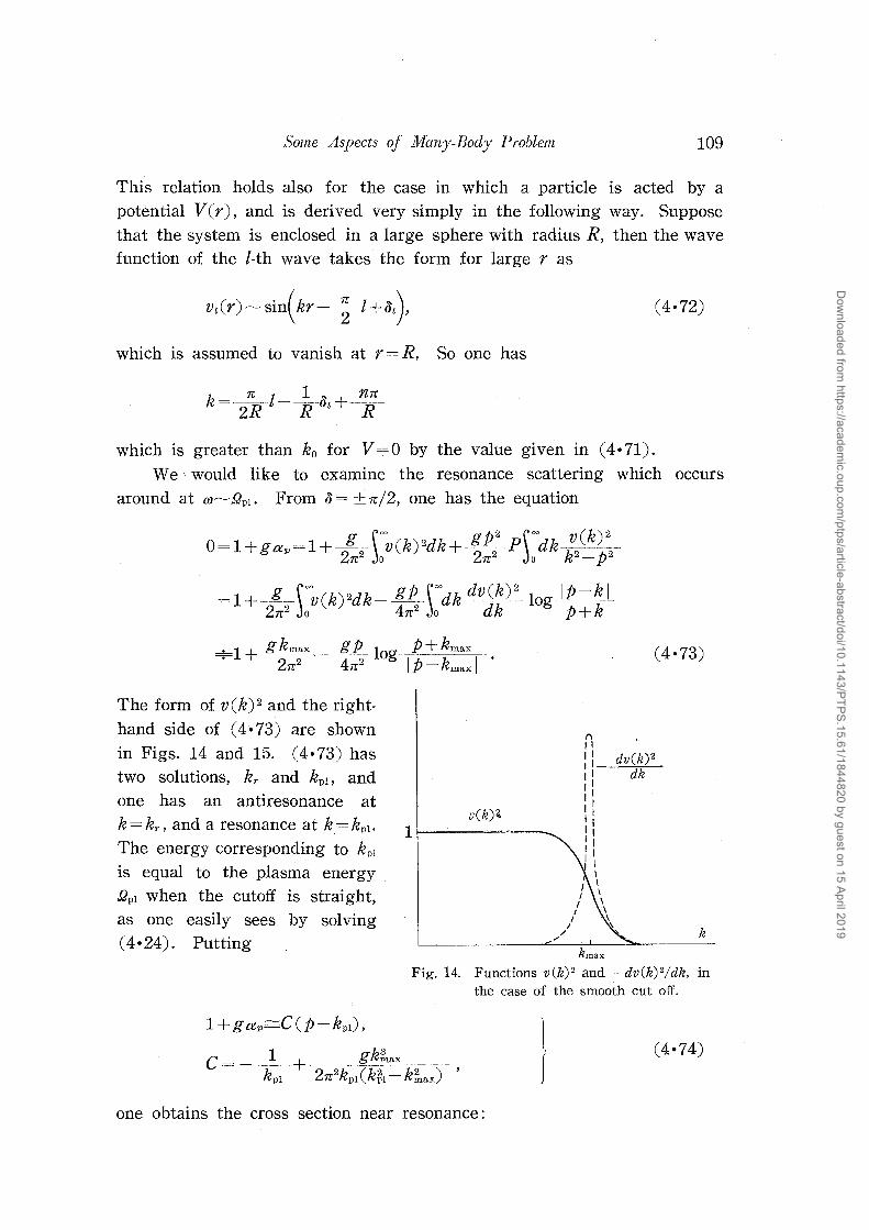
Some Aspects of Many-Body Problem 109
This relation holds also for the case in which a particle is acted by a potential V(r), and is derived very simply in the following way. Suppose that the system is enclosed in a large sphere with radius R, then the wave function of the l-th wave takes the form for large r as
(4·72)
which is assumed to vanish at r = R. So one has
k = ___ !£_ l - _1 __ 8t + __ f/,!E_ 2R R R
which is greater than ko for 0 by the value given in (4•71). We would like to examine the resonance scattering which occurs
around at (l)~QPl· From 8 = + n:/2, one has the equation
1 _g __ .\~v(k) 2dk gpJ=dk dv(k) 2- logJt__j?_L
2n:2 Jo 4rr2 Jo dk P+ k
+-g-~~;~ -{~-log ~~-±Z::~~--.
('\
II
(4•73)
The form of v(k) 2 and the righthand side of ( 4 • 73) are shown in Figs. 14 and 15. ( 4•73) has two solutions, kr and kpr, and one has an antiresonance at k=kr, and a resonance at k=kp1•
The energy corresponding to kp1
is equal to the plasma energy QPI when the cutoff is straight, as one easily sees by solving ( 4 • 24) . Putting
I: dv(k) 2
,, dk
c
v(k)'4
,, ,, I I II II I I I I I\
I I I I \ \
kmax
~
k
Fig. 14. Functions v(k) 2 and -dv(k) 2/dk, in the case of the smooth cut off.
I f
(4·74)
one obtains the cross section near resonance:
Dow
nloaded from https://academ
ic.oup.com/ptps/article-abstract/doi/10.1143/PTPS.15.61/1844820 by guest on 15 April 2019

110
1+ gkmax 27!'2
l
N. Fukuda and Y. Wada
I I I I I
---:-----------1
I I
k
Fig. 15. The right hand side of (4•73) as a function of k. kr gives the wave
number of an antiresonance and kpl gives that of a resonance.
~ 4n: g 2fi~l ------ C2k~1· • ·c:;p- JJpl) 2 + g-2[3-glj C2 . (4·75)
The resonance half-width is given by
(4·76)
and tends .to zero as the cutoff becomes sharper. For a straight cutoff one has a plasma state instead of resonance scattering.
One will now look for the unitary operator U for ( 4•18) 33\ i.e.
satisfying
Let us introduce a matrix S defined by
[t)=S T ' Ak1 ak1 . . . . . .
and matrices r; and r:;, of the form
(
1 : 0 r; •. : . ..•.. J '
0: -1.
Then the conditions ( 4•19) give
S=[ ~ .. : .. ~. J, 75* • ""* P :a
(4·77)
(4·78)
(4·79) '
Dow
nloaded from https://academ
ic.oup.com/ptps/article-abstract/doi/10.1143/PTPS.15.61/1844820 by guest on 15 April 2019

Some Aspects of Many-Body Problem 111
r;Sr;S* 1. (4•80)
Multiplying S- 1r; from the left and r;S from the right, one obtains
r;S*r;S = 1,
From the form of S in (4·78) it follows that
t:S= S*C:, t:S* sc:, t:S* sc:. Introducing the matrix K defined by
S=eK , one has
K* -r;Kr;, r;K* Kr; 0
(4•81)
(4•82)
(4•83)
(4·84) '
on account of (4•81), which means that r;K is antihermitian. From (4•82) and ( 4•84) follow
C:KC: -r;Kr;, r;K= -C:KC:r;. (4·85)
If one defines a column "vector" b and a row vector b* by
(4•86)
one has the following commutation relations:
[b;, bn1] = -r;nn', (4·87)
where
~ ( .. ~ ... = .. ~ l· -1:o
(4·88)
Eq. (4·87) leads, for an arbitrary c-number vector X, to
[b*, (X*b)] X*r;, [b, (X*b)] ~X. (4·89)
Let us show that
(4·90)
is a desired unitary operator, i.e.
(4•91)
To this end, one makes use of an identity
Dow
nloaded from https://academ
ic.oup.com/ptps/article-abstract/doi/10.1143/PTPS.15.61/1844820 by guest on 15 April 2019

112 N. Fukuda and Y. Wada
(4·92)
which can be proved by the mathematical induction. For n = 0, one has
[b*r;Kb, X*b] b*r;K~X- X*r;YJKb
b*(KX-X*Kb bKX-X*Kb 2X*Kb,
where one has used some identities derived above and
(4·93)
In terms of the unitary operator U, a complete set of eigenfunctions are given by
(4·94)
It is difficult, however, to obtain an explicit formula for U. Let us now instead introduce an operator V such that V contains only creation operators and satisfies
where c is a constant. One assumes that V has a form
and notices that
0= (aa+[3a*) Vzt>0 = (aa+[3a*)exp(a*Ga*)<Po.
On account of
exp( a*Ga*) • (aa) •exp(a*Ga*)
=aa- [_(a*Ga*), aa] =aa+2aGa*,
one obtains from ( 4 • 97) an equation to determine G:
[3+2aG 0,
(4·95)
(4·96)
(4·97)
(4·98)
(4·99)
It is to be noted that c V is also obtained by decompositing U into normal products and retaining those terms which include no annihilation operators. A complete set of eigenfunctions are given by
(4•100)
Eq. ( 4·99) is a typical Wiener-Hop£ equation and can be solved analy
tically.
Dow
nloaded from https://academ
ic.oup.com/ptps/article-abstract/doi/10.1143/PTPS.15.61/1844820 by guest on 15 April 2019

Some Aspects of Many-Body .Problem
Introducing (4•22) into (4·99), one obtains
which, for a fixed I, is of the form
v(l) V2;;~ '
113
(4•101)
(4·102)
with unknown {Xm'}. It can be shown at the end of this paper that
Gkl v(k )v (l) 1 (mk +aJv) (mz +mv) (4•103)
2Q -v4-;~M=-II~··--········-·---·----~-·····-·-·--
mk + mz p (mk +SJp) (mz +SJp)
v(k)v(l) 1 (J)k + mmax mz -~-··~·--·--·-.. --.. -~~~-·--·-"·--· ~
2Q -v4;~;~-- (J)k + mz (J)k + SJpl (J)z +SJpl
§ 5. Theory of an electron gas (1)
As already pointed out in the Introduction, the electrons in a metal are capable of displaying both individual and collective behaviors, and the key to this dualism is the understanding of correlation effects resulting from the interaction between the electrons. The quantum mechanical approach to the plasma oscillation was first developed by Bohm and Pines,8
)
and was applied to the electron theory of metals with great success. We will not go into this theory, but rather explain the recent theory of GellMann, Brueckner, Sawada and others,9
),lO) which is exact at high density and is suggestive from the viewpoint of many-body problem.
The electron-phonon interaction is quite weak, and can be neglected in the first approximation. Electrons in a periodic lattice lead to the effective mass and to the band structure, but we will adopt throughout this section a simplified model for a metal in which we replace the effect of the ionic fields by a uniform background of positive charge. Deviation from this model should be taken into account later on. If we neglect the Coulomb interaction, the energy of an electron with momentum k is given by mk k 2 /2m. The electronic specific heat is determined by the level density at the Fermi surface and is proportional to T at low temperature in the free electron model. This is in good agreement with experiments. However the cohesive energy per electron becomes positive as given by
(5·1)
where E1!' is the Fermi energy per electron and in the Rydberg unit
Dow
nloaded from https://academ
ic.oup.com/ptps/article-abstract/doi/10.1143/PTPS.15.61/1844820 by guest on 15 April 2019

114 N. Fukuda and Y. W ada
2 2.21 . ---- ---.-----
5a2r~ r~
a (4/9n) 113, rs r0 /a, (5•2)
where ro is the radius of the spherical volume occupied by an electron which is defined by
N -~-~=p=
Q k~· _ (····4n )-l -s - 3 ro ' (5·3)
and a is the Bohr radius (1/me2). Cion is a constant which is the difference between the binding energy of the lattice for the most tightly bound conduction electron and the ionization energy of the free atom, and can easily be calculated.
If we take into account the Coulomb interaction in the Hartree approximation according to the method of Wigner and Seitz/4
) we have an extra term 1.2/rs in (5•1):
su= so+ 1.2/rs. (5·4)
In an approximation which takes into account the exchange effect, the energy of an electron having a momentum k is given by
(J)(k) (5·5)
and the cohesive energy becomes
eull eu 0•916/rs, (5•6)
which is negative and closer to experimental value. However, the exchange term in (5•5) profoundly alters the predictions of the independent electron model, since the density of states at the Fermi surface vanishes. For instance, the temperature dependence of the specific heat is changed from a linear relation to one of the form T /logT.4
)
We would like to note here that the cohesive energy obtained above should give the upper bound for the true value e, because it is the result obtained by the variational method using the plane wave trial functions. The difference between s and eull is called the correlation energy. Any improved approximation should give a negative correlation energy. It is easy, on the other hand, to calculate the lower bound of the correlation energy. Since E1'' is the lowest bound of the kinetic energy of an electron gas, we can obtain the lower bound of the total energy if we know the lowest bound for the Coulomb energy. The latter leads to an extra term in ( 5 • 4) which was calculated by Winger: 35
)
Dow
nloaded from https://academ
ic.oup.com/ptps/article-abstract/doi/10.1143/PTPS.15.61/1844820 by guest on 15 April 2019

Some Aspects of Many-Body Problem
1.8 ew=eH- ----. rs
So the correlation . energy is
0.88 rs
115
(5·7)
(5•8)
This is exact in the low density limit rs-?oo and is extrapolated to medium density as
1.8 ew' = e~u-- --- · · . rs+7.8 (5·9)
In Table 1, we show those calculated values and experimental results for the alkali metals.3
6)
Table 1. Cohesive energy of the alkali metals.
Metal m*/m rs cion CH CHF eexp
Li 1. 45 4.5 87.2 74.4 17.0 -36.5
Na 0.98 3.8 -71.3 67.6 -6.8 -26.0
K 0.93 4.4 -51.6 56.1 -4.3 -22.6
Rb 0.89 4.5 -47.6 53.4 -3.4 -18.9
Cs 0.83 4.3 -43.9 49.9 -2.9 -18.8
Let us now formulate the theory of an electron gas in a uniform positive background. The Hamiltonian of the system is given by
where H0 is conventional kinetic energy and
Hr ---~- ~d3xd3x''fr* (x)o/* (x')v (x- x')o/(x')o/(x),
Hex ~d3Xo/* (x) o/(x)Vex(X),
Hp= ~2
~d3xd3x'v(x-x'),
v(x)
(5·10)
(5·11)
Hr is the Coulomb energy of the electrons, Hex the interaction energy between the electrons and the positive background, and Hp the self-energy
Dow
nloaded from https://academ
ic.oup.com/ptps/article-abstract/doi/10.1143/PTPS.15.61/1844820 by guest on 15 April 2019

116 N. Fukuda and Y. Wada
of the latter. In the hole theory formulation, the function o/(x) is expan:ded as
and the total Hamiltonian is decomposed into normal products as
where
H 1=-}- ~d3Xd3x' :o/*(x)o/*(x')v(x-x')o/(x')'t(x):,
H 2 = ~d3xd3x'D_(x x')v(x x'):o/*(x)o/(x'):,
U=EF- ~d3xd3x'v(x-x')D:.(x x'),
1 ~ e-ik(x-x')s-kl Ucra'•
!J k<kF
(5·12)
(5·13)
(5·14)
In the last expression, a and a' denote the spin indices of 't(x) and o/*(x'),
respectively, and the sum over k is carried out only on momenta. The
ordinary Coulomb energy is exactly canceled, and one easily obtains
H 2 = ~ Llwka: ak-~ Llwkb~bk , k>kF k~kF
-~-~-F~[ 1 + ~lkk:2
log I Z±Z;T J · (5·15)
The first term of U gives 2.21/r~ and the second -0.916/rs per electron. From the dimensional analysis, one finds that the correlation energy
ec per electron is, in the Rydberg unit, a function of rs alone. Since rs is
proportional to e2, the second order term is proportional to rg, the third to
rs, and so on. It may seem, therefore, that in the high density limit, rs---'»0,
it is sufficient to calculate only the second order term. As a matter of
fact, the exchange second order term (e12)) is constant and gives
(5•16)
while the ordinary second order term efP is logarithmically divergent for
low momentum transfer q as
e~2 ) =0.12441im logqmin +const. (5•17) qmiu->0
Dow
nloaded from https://academ
ic.oup.com/ptps/article-abstract/doi/10.1143/PTPS.15.61/1844820 by guest on 15 April 2019

Some Aspects of Many-Body Problem 117
The coefficient of rs in the third order term is quadratically divergent like 1/ q'tnin , and in a· similar way one has
ec 0.046+ (log. divergence) +rs(quadratic div.)
rHquartic div.) (5·18)
According to Bohm and Pines,Bl the Coulomb potential is screened and
qmin ~ (con st.) r¥2 +higher orders in r s • (5·19)
If this were true, one might anticipate that
ec 0.046+0.0622logrs+C, (5·20)
in the high density limit, where C is a constant to be calculated from all the most divergent higher order diagrams.
In order to identify the most divergent diagrams, let us introduce the interaction representation by
Then, according to (2•37) the correlation energy is given as
Denoting the denominator as <S>o, one obtains
= -iTxthe numerator of (5•22),
where T is the time of the whole world, and
(5·21)
(5·23)
(5·24)
Now <S>o can be reduced to the sum of contributions from the linked diagrams only. Let us denote those from the r-th order linked diagrams by <S>tr:
Dow
nloaded from https://academ
ic.oup.com/ptps/article-abstract/doi/10.1143/PTPS.15.61/1844820 by guest on 15 April 2019

118 N. Fukuda andY. Wada
00
<S>t= ~<S>&r, (5·25) r~o
and consider an n-th order diagram of <S>o in which there are n2 linked diagrams of second order, ... , ni linked diagrams of i-th order, and so on. Then the number of ways to divide n vertices into the groups, which contain (2n2), • • ·, (ini), .. · vertices respectively, is equal to
and the number of ways to divide int vertices into ni groups each of which contains i vertices is
These are all equivalent diagrams, and one obtains in this way
X {L<T(Hi(tt)Hi(t2))>o} ... {L<T(Hi(t2n2-t)Hi(t2n2))>o}
X {L<T(Hi(f2n2+t)Hi(t2n2+2)Hi(t2n2+s))>o} ...
= 1 = ~ ~ {<S>82}nz, .. {<S>Bi}nt,,.
n=O :Sin1=n n2 '' 'Jiti i
from which it follows that
(5·26)
(5·27)
We are now in a position to analyze the degree of divergence for any of the linked diagrams. The propagator of a free electron is defined by
J 1/(ko-mk+ie);
ll/(ko-mk-ie);
(5•28)
(5·29)
Dow
nloaded from https://academ
ic.oup.com/ptps/article-abstract/doi/10.1143/PTPS.15.61/1844820 by guest on 15 April 2019

Some Aspects of Many-Body Problem 119
In calculating the contribution from a Feynman diagram in momentum space, the following rules are to be applied.37
)
1) Associate i/ (2rc) 4 • iJcrcr'S(kfJ.) to each electron line. 2) Associate (2rc) 5e2/ q2 or (2rc) 4L1(l)k to each vertex according to H 1
or H 2, where q is the momentum transfer. 3) Give positive or negative sign according to the even or odd permu
tation of t' and t'* in (5 • 25). 4) Take trace with respect to spin variables and integrate over all
independent momenta and energies. 5) Multiply QT / (2rc) 4 corresponding to the total energy and momen
tum conservation.
As an example, Feynman diagrams corresponding to second order terms in H 1 are shown in Fig. 16. For the exchange diagram one has
.,.(2) <;;./)
which gives (5•16) in the Rydberg unit. Suppose that we have an
n-th order Feynman diagram in which all interactions are of H 1 type. It consists of 2n real lines expressing elect- k1 + q
rons or holes and n broken kz-Q
lines denoting the interaction. At each vertex one has ,the conservation of energy and momentum, but one of them
Fig. 16. Second order diagrams for the ground state energy. The left diagram gives e~2 l
and the right e~2 ).
simply gives the over all conservation. Therefore the total number of independent energy-momenta is 3n- (2n -1) = n + 1. Let us assume that there are m real closed curves in the diagram, and assign an energymomentum ki to one line in the i-th closed curve. The remaining independent (n+1-m) energy-momenta, Q1, Q2, ... , Qn+l-m, are assigned to some of the broken lines by taking into account the energy-momentum conservation. Since the integrations over the energies are easily performed, one may consider only the momentum integrations. The result is identical with that of Hugenholtz and Van Hove. There are two elements in the integrals, one that strengthens the infrared divergence and the other that suppresses it. The former comes from: 1) 1/q2 terms associated with the broken lines. Evidently, this does not
exceed an order (2n). 2) The denominators which vanish when some momentum transfer q is
Dow
nloaded from https://academ
ic.oup.com/ptps/article-abstract/doi/10.1143/PTPS.15.61/1844820 by guest on 15 April 2019

120 N. Fukuda andY. Wada
put to zero. Since the intermediate states that make the energy denomi
nator vanish are restricted to those in which the excitation energy of
each pair involved can be made infinitesimal for zero momentum transfer,
all the momentum transfers appearing in those intermediate states should
have the same value q. If the number of such states contained in a
diagram is s, then the order of singularity leading to the infrared diver
gence is at most 2n +s.
Time
ks-H St----~------------_,~-----------
----
1~---~---+-r------------------------k2
ql
Fig. 17. An example of a diagram which makes the degree of divergence higher
in s order due to the energy denominators.
The elements which suppress this divergence are:
1) The integrals over d3ki. The domain for each of these integrals which
are connected with the above mentioned s energy denominators is pro
portional to q, and the order of divergence is reduced by the order of
s+l. 2) The integrals over d3qi. These are 3(n+1-m)-fold.
Therefore the degree of divergence is not higher than
(2n+s) -- (s+1) -3(n+l-m) =--= -n+3m-4. (5•31)
Since m<n, the maximum value of this is
2n- 4 which corresponds to a diagram as
shown in Fig. 18.
We have considered so far only the
contributions from H 1• If there are p inter
actions of H 2 type in an n-th order diagram,
the total number of real and broken
lines is 3n-2p, the number of effective
energy-momentum conservations 2n- p l,
that of independent energy-momenta n-p + 1
and that of independent momentum
-------------------0 -------
Fig. 18. An example of the most divergent diagram (fourth order).
Dow
nloaded from https://academ
ic.oup.com/ptps/article-abstract/doi/10.1143/PTPS.15.61/1844820 by guest on 15 April 2019
Some Aspects of Many-Body Problem 121
transfers n -- p 1 m, m being the number of the real closed curves.
Therefore the order of singularity is 2(n---p) coming from 1/q2 plus (s+P) from the energy denominators. The order of suppression is (s + 1) due to dkt integrals plus 3(n-P+1 m) due to dqt integrals. Thus the degree of divergence is at most
2(n-p) + (s+P) (s+1) 3(n-P+1 m) n 2P 4 3m. (5•32)
Since m<n-p, the maximum value for this is (2n-p-4) and the most divergent diagrams correspond to P=O, that is, include no H 2 type interactions.
Keeping these considerations in mind, one can sum up the contributions from all the most divergent diagrams up to infinite order as follows. Let us first define the Fourier transform pq of the density operator as
pq = ~d3xo/* (x)o/(x)e-iqk
= ::E {a:ap+q +bpap+q +a:b:+q +bpb:+q}. p
Then, from (5•14) one has
(5•33)
(5•34)
Since the most divergent diagrams consist of the processes in which a pair of electron and hole is created and annihilated, one can consider pq as a field operator describing the behavior of the pair. Defining the propagator of this operator by
where
Dq(t-t')oqq'=<<Po I T(:pq(t): :p_q,(t') :) I <l)o>
a ,_!_\00
d;.D ().)e-iA.tt -t') qq 2ni j_"" q '
___ 1 __ ---:--- + 1 U>p+q- lOp-).- U>p;-q- lOp+).-
(5·35)
(5•36)
one applies the Wick theorem to the S-matrix,37) thus obtaining the contri
butions from the most divergent diagrams as
Dow
nloaded from https://academ
ic.oup.com/ptps/article-abstract/doi/10.1143/PTPS.15.61/1844820 by guest on 15 April 2019

122 N. Fukuda andY. Wada
_i -b \00 d;.[ 4n:e2~ Dq (A) 4n:N q J -oo !Jq
It is to be noticed here that the operator pq (t) is treated as a whole and should not be broken into a and b's in the high den-sity limit. Since the integrand of (5·37) vanishes as 1/ I J.l 2
as I J.l goes to infinity, the path for ). integration can be closed with a large semi-circle on the lower half complex plane as shown in Fig. 19. Let us call this path C. Then the first
X X X X X
(5·37)
i.-plane
X X X X X
c
term of (5 • 37) gives, by calculating the residues of the poles in the lower half plane,
Fig. 19. Path for A. integration in (5•37) and the locations of singularities of the integ· rand.
(5•38)
Denoting the roots of the equation
by !Jj;l(q) and !Jk+)(q) which are on the upper and lower half plane respectively, one has
).-const•II
P J.+wp+q-wP-Ip+ql>kF p~kF
Therefore the second term in (5•37) becomes
which leads, together with (5•38), to the correlation energy
ec 2}v ~ {!J~+l (q) -wp+q +wp
[p+q>kpf p~kF
_ 8n:e:_ } + eb(2)
!Jq2 ' (5·41)
Dow
nloaded from https://academ
ic.oup.com/ptps/article-abstract/doi/10.1143/PTPS.15.61/1844820 by guest on 15 April 2019

Some Aspects of Many-Body Problem 123
where the summation over spin variables is already taken. Since Dq (A) has no poles in the upper-right and lower-left planes, one
can transform the path of J. integration in (5•37) to the imaginary axis,
thus obtaining
ec-e~2l= --1--~\"' d;.~J:-(~ 4rce: -Dq(i;.))n, (5•42) 4rcN q ~-"" n=z n t2q
where
(5·43)
In the high density limit, one gets from (5·42)
~ (1-ln2) (1n-4ar~_ 7C2 7C
1.051) 0.0508.9) (5•44)
It is to be noted that the contribution from plasma states to the correlation energy is explicitly seen in the form of (5•41), but not in (5•42).
§ 6. Theory of an electron gas (2)
The theory by Gell-Mann and Brueckner discussed in the previous
section does not seem to give any satisfactory result when applied to a low
density system as the actual metal. However, it has succeeded in showing
the fact that the difficulty of the infra-red divergence can be overcome if
the Coulomb interactions between the electrons are correctly taken into account, the interactions being effectively screened. Meanwhile, Bohm and
Pines had considered the screening of the interactions to be due to collective motions of the electrons, plasma oscillations. s) When an electron
impinges upon the metal the other electrons tend to recede. Thus the
surroundings of the electron are charged up positively, screening its Coulomb
field. This receding motion of the electrons is to be interpreted in terms
of the plasma oscillation. As we have not explicitly used the notation "plasma oscillation" so
far, it is important to consider whether the screening of the Coulomb
interaction given by Gell-Mann and Brueckner is due to the electronic collective motions or not. Sawada et al,lol,ll) and WentzeP2) have made
clear discussions on this point. A simple review for their theory will
be first given here. Sawada considered to transform the restrictions upon diagrams to the most divergent ones into the conditions for the Hamiltonian. The terms in the interaction energy which give rise to the most divergent diagrams are those that create or annihilate two pairs of
electron and ho1e simultaneously and those that make a pair scatter jnto
Dow
nloaded from https://academ
ic.oup.com/ptps/article-abstract/doi/10.1143/PTPS.15.61/1844820 by guest on 15 April 2019

124 N. Fukuda andY. Wada
another. Such terms in 1/1 will be denoted by He which takes the form
(6•1)
He involves something unnecessary yet. For instance, it involves the exchange interaction between electron and hole in which we are not interested except for the second order. In most divergent diagrams one considers only those intermediate states which involve the pairs with common momentum transfer. In such cases the operator a;+qb; behaves just as an creation operator of a pair with momentum transfer q. Those with different q commute with each other, and one has
(6•2)
The parentheses on the right hand side may be replaced by unity, since the system with repulsive interaction is expected to have a particle distribution which is not so drastically different from that of degenerate Fermi gas. The correction for this approximation can be estimated by means of the spin description of the system.19
) Now the operator
satisfies the commutation relations of Bose particles
[ cp c q), c;, c q') J ::--= app'aqq' ,
[Cp(q), cp,(q')J =O.
And (6•1) can be rewritten in terms of them as
(6·3)
(6•4)
- :~~~~~~~~~~~- b ~[b {C; ( q) + C_P ( -q)} b {CP' (q) + C:P' ( q)} J Q q q p P'
4ne2 1 Q
(6·5)
The kinetic energy is now found to be391
(6•6)
Although it may seem that we have counted every term of Ho in (5•14) many times in (6~•6), it is not true since those with different q's operate on different states of the system. Thus the Hamiltonian is reduced to that of a Bose system
Dow
nloaded from https://academ
ic.oup.com/ptps/article-abstract/doi/10.1143/PTPS.15.61/1844820 by guest on 15 April 2019

Some Aspects of Many-Body Problem 125
U+Nd2 )+Ho+Hc, (6•7)
which was derived by W entzeP2) and to which the second order exchange
energy Ne62) is to be added. (6•7) can be exactly diagonalized just as the
neutral pair theory discussed in section 4, and gives the ground state energy identical with that derived by Gell-Mann and Brueckner. We have now one plasmon mode for each momentum transfer q. As ( 4·18), a creation operator for each normal mode can be written
(6·8)
in which app'(q) and £jppr(q) take the forms,
tXppr(q) Np(q) !Jp ( q~) + Wpt + q _:-;;; •
(6·9)
!Jp (q) is the frequency of the normal mode p, q which is given by the root of the equation
(6·10)
and N P ( q) takes the form
N (q) = 1~8-;(l~jQ~;(-q)- (6•11) P V t2q2 8e 2 •
Let us first consider ( 6 • 8) for a scattering normal mode. As JJp ( q) is close to one of the energies of one pair states wp'- wp' -q, some app' ( q) 's make a large contribution to ( 6 • 8). Therefore, it is natural to regard this mode as an one pair excitation mode rather than a collective excitation of the electrons. In fact, the excitation energy of the scattering mode can be correctly obtained by introducing the interaction into the free one pair state as was shown in the example of the neutral pair theory. Meanwhile, in the case of the plasmon mode, fJp1(q) is larger than the energy spectrum of any of the one pair states. So there is no special app' (q) which makes a large contribution to (6•8), one plasmon state being the superposition of various pair states. Thus this mode may be considered to be an excitation of some collective motion of the electrons. In this way it becomes evident that Gell-Mann and Brueckner theory involves the collective motion of the electrons considered first by Bohm and Pines. Strictly speaking, the collective motion is slightly different from that of density fluctuation, since a and e's in (6·9) depend on p'. The plasmon with long wave length asymptotically tends to the density fluctuation.
As we have the Hamiltonian (6•7) which is regarded as exact in the high density limit, it may seem that we can obtain a correct result not
Dow
nloaded from https://academ
ic.oup.com/ptps/article-abstract/doi/10.1143/PTPS.15.61/1844820 by guest on 15 April 2019

126 N. Fukuda andY. Wada
only for the. ground state but also for the excited states. However, this is not the case. The energy shift of the scattering mode is inversely proportional to the normalization volume which can be derived as in section 4. Therefore, the energy spectrum coincides with that of the free system when the system becomes large. Meanwhile, if the interaction is taken into account by means of the perturbation theory, one obtains a finite energy shift Ll(J)p Ll(J)p-q even in the lowest order term. This suggests the fact that Sawada-Wentzel's Hamiltonian has missed important terms for the excited state. And these terms must have an essential effect for the low temperature specific heat of the system. Well, then, what are the most effective terms for the excitation energy of the system? Gell-Mann40
)
has first discussed this question. The energies of excited states would be estimated by introducing adiabatically the interactions into the freelyexcited states. Excited particles and holes interact with the medium and with each other. In the case of low excitation the former makes the predominant contribution, since the number of excited particles is negligibly small in comparison with that of unexcited ones. We may merely take into account such diagrams that involve only the so-called self energy parts as illustrated in Fig. 20. Meanwhile, the Hamiltonian derived by Sawada and Wentzel (6•7) takes into account only the contributions of those diagrams illustrated in Fig. 21, since their Hamiltonian has been constructed so as to consider the effect of the most divergent diagrams. As these diagrams do not belong to desired ones, the contribution to the frequency correction has vanished when the normalization volume becomes large. Now the energy of the system can be written
Fig. 20. An example of the diagrams which make predominant contribution for the excitation energy. P1 electron line involves the second order self energy part.
(6•12)
PtP2
v _____ o rr ___ _ Pt P2
Fig. 21. An example of diagrams which give the excitation energy calculated from Sawada-Wentzel's Hamiltonian.
* The symbols (a) and (b) will be used to designate the particle and hole states, respectively.
Dow
nloaded from https://academ
ic.oup.com/ptps/article-abstract/doi/10.1143/PTPS.15.61/1844820 by guest on 15 April 2019

Some Aspects of Many-Body Problem 127
where Eo the ground state energy, and pjal(pjb)) are the momenta of the particles (holes) excited in the free system. Then the specific heat per electron (at constant volume) takes the form41
)
(6·13)
where k is the Boltzmann constant, T temperature and e the energy of a particle in the Rydberg unit.
As e(p) is the energy of a particle (hole) in the medium of N e]ectrons, it is to be obtained by means of the analytical properties of the so-called "one particle Green's function". It is defined by
S~(x-x', t-t')=<Wol T('o/H(x,t)'o/l;(x',t') IWo>, (6•14)
where 'tT:l:(x, t) and 'o/l;(x', t') are the operators for the electron field in the Heisenberg representation. The space-time dependence of the field quantity can be made explicit in terms of the Hamiltonian H and the momentum p as follows:
'o/H(X, t) = e-ipx+iHt1frH(O, O)e-iHt+ipx.
A complete set of eigenstates is denoted by 'I'n which satisfies
The Fourier transform of (6•14) now takes the form
S' (kP.) 7- ~e-ikx+ikotS~(x, t)dxdt
where p~ and p~ are defined by
p~
Q
(6·15)
(6·16)
(6·17)
(6•18)
(6•17) and (6•18) show that the poles of S'(kp.) under the real axis give the energies of one particle ( + pairs) states, while those above the real axis give the energies of one hole ( pairs) states with inverse sign.
As is well known, the one particle Green's function satisfies an integral equation. If (6•14) is calculated by making use of the adiabatic theorem, it is to be obtained in a series of "proper self energy parts". Proper self energy part is the self energy part, which cannot be separated into the sum of two self energy parts and is denoted by .:E ( y y', t t'). One
Dow
nloaded from https://academ
ic.oup.com/ptps/article-abstract/doi/10.1143/PTPS.15.61/1844820 by guest on 15 April 2019

128 N. Fukuda andY. Wada
particle Green's function now satisfies the equation
SJr(x x', t t') sli'(x-x', t t') + ~dy'dy"ds'ds"SF(x-y', t s')
x :::S (y'- y", s'- s") SJr (y" x', s" t'), (6·19)
which can be rewritten as an equation among the Fourier transforms,
Here :::8 (k/).) is defined to be
:::8 (kM) = i~dxdte·- ikx-1-ikot:::S (x, t).
(6•20) gives
(6·20)
(6·21)
(6•22)
Thus the single particle energy s(k) =Ek-Eo is obtained as the solution
of the equation,
(6·23)
for the unknown ko. :::S (kM) may be computed in the form of the power
series in rs in the high density limit. Then the power series for e(k)
will be derived by the iterated solution of (5•30).
(6•24)
DuBois42) has made use of this formula to discuss the correction for specific
heat in detail. He has derived it up to the order rg. However we will
here consider only up to order r;s 1, since we are mainly concerned with
the anomalous effect of the exchange term. Then (6·24) is sufficiently
well approximated by the first two terms, and :::S (k,J needs to be calculated
up to 1/rs order. Among the various proper self energy parts, which one
will make the contribution of order 1/rs? It can be seen by repeating the
similar analysis with those applied for the correlation energy in section 5
that the desired proper self energy parts are such as illustrated in Fig.
22. As these diagrams involve one less closed loops than the corresponding
most divergent diagrams for the correlation energy (Fig. 18), the degree
of divergence is higher by one order, that is, the n-th order term of the
perturbation series diverges in 2n- 3 order. If the cut-off for the momen
tum transfer is assumed to be Qmin~rS/2, the contributions for e(k) is of
the order of magnitude r;s11 2• Meanwhile, the contribution from the first
order term of the perturbation series is of the order of magnitude r:S 1•
Dow
nloaded from https://academ
ic.oup.com/ptps/article-abstract/doi/10.1143/PTPS.15.61/1844820 by guest on 15 April 2019

Some Aspects of Many-Body Problem 129
Thus it may seem that the contributions from the higher order terms are too small to compensate that of the first order and the anomaly of the low temperature specific heat remains unex-plained. However, the required quantity is the level density at .the Fermi surface as indicated in (6•13). The differentiation of the excitation energy by the momentum may not change the rs dependence if the former is a convergent quantity. Since it is a divergent quantity, the order of the divergence is increased by one order. In this way, the most divergent diagrams will give r:S 1 order contributions for the level density.
Now we will calculate ::S (kM) given by the most divergent diagrams. ::S (x, t) now takes the form
::S (x, t) e2
i --1 ·x-
1
-- D _ ( x) ~ ( t)
---------- ------0
Fig. 22. Most divergent dia· gram for the proper self energy part. Example of the fourth order.
(6·25)
in terms of the notations in ( 5 •14) and ( 5 • 35). The first term on the right hand side is the contribution of the first order term of the perturbation series, and the second term is the sum of those of the diagrams illustrated in Fig. 22. The Fourier transform of (6•25) is calculated according to (6•21), and is derived to be
(kM) LiaJk -(2~)-4 ~dqdqoS(k q, ko Qo) 4
ne2
• r£~ft;~~~~~~!(~o), (6•26)
by means of (5·15), (5•28) and (5·35). The path for q0 integration may be closed with a large semi-circle on the lower half plane, since the contribution along the semi-circle is evidently negligible. If the integrand is rewritten in the form,
( 4ne2 / Qq 2) Dq (qo) ·1 +-r4~e2/.f2q 2)Dq(qo)
1 1 1 + (4ne2/tJq2)Dq (q0 ) '
the first term on the right hand side just compensates LiaJk in (6•26). The path for the integration of the second term may be taken to c given
Dow
nloaded from https://academ
ic.oup.com/ptps/article-abstract/doi/10.1143/PTPS.15.61/1844820 by guest on 15 April 2019

130 N. Fukuda and Y. Wada
in Fig. 23 that is along the imaginary axis and the large semi-circle on the right half of the q0 plane. Then the singularities of Dq (q0 ) make no contributions to the integral as seen from Fig. 19. The pole of S(k-q, ko-qo) makes a contribution only when k0 -m~a2q>O or k0 -m~b2q<O. So b (k"") can be rewritten
ko- (o~a_::q + ic: X
X
ko-oJ~"}_q -ic
Fig. 23. The path for qo integration in (6•27).
b (kM) = -T2~) 4 ~dq ~c dqoS(k -q, ko -qo)-~;~:~. -r+ -c;4;e2 11(]25.0~ (l]~5 + .. (2~) 3 ~ dq~'!jf:_ h-+ ( 4~ef;~~i) n~+~o -=~~2-;)
fJ(mi:'2q·····ko) } ... ···-··· 2----2-~--~---- -(b) ..... '
1 + ( 4ne I Qq ) Dq (ko -mk-q)
where fJ(x) is defined by
f 1 if x20 fJ(x) l o: if x<o.
( 6 • 27) may be transformed to
(6•27)
(6•28)
b (kM) =- --(2~)4·-~dq j:~~2
-~~~qv (ko komk::)i+ q5 i -+·C~i~e2 I ~q2) Dq (iqo)
2(f"n) 3 -~ dq 4;;
2
+second term on the right hand side of ( 6 • 27).
(6·29) This is the proper self energy part composed of the most divergent diagrams. The single particle energy given by the first two terms of (6•24) is now found to be
Dow
nloaded from https://academ
ic.oup.com/ptps/article-abstract/doi/10.1143/PTPS.15.61/1844820 by guest on 15 April 2019

Some Aspects of Many-Body Problem 131
e(k) = a~~~+ ~r~~s[~dq ~ ~~~A(q2~L~i~~~;4q2,12 •f-1=-~~r~~~q25Q~(~) -~ ~dq-:2 +n ~ ~~ {1+ ::qs2 ~ dp(q2 +(:.p -k)-+(q•:+k))
k> II{-q l>l I p+q 1>1 P<l
+i arfj__ r dpo(q2 + (q•p-k))} (6·30) nq2 j
Jp+qJ>l P<l
in Rydberg unit where the relation between Dq(iq0 ) and Qq (5·43) is used. The angular integrals in the first two terms can be performed, and give the result,
which may be rewritten, by making use of the relation,
in the form,
- _21!li ~: dq[~~~A log-~~+ ;~}:!4J2 {-r+-c~-~~~-2l]2)Q~(J:5 1}
+2n(2k-q)o( k--~--) J
(6·32)
-~k- ~: dq~~~J log-~~-+-~~}~+J~: {1 +T~Y.~/:2q2)Qq(X) 1} 2n2k.
(6·33)
As we are interested in the terms up to the order r:S\ the integrand in (6·33) may be expanded in the power series of q and the integration can be taken from q=O to q'""l. In such a case Qq(A) can be replaced by
Qq(A)::::::::.4nR(A) 4n [1 ,1 arctanr 1],
as was done by Gell-Mann and Brueckner. The first term in (6·33) is now written as
2ar s \"" dJ --· R (A) log 1 ± __ (i0C?'s~ n:) f?:(J) J-= +k2 (4ars/n)R(A) '
(6·34)
Dow
nloaded from https://academ
ic.oup.com/ptps/article-abstract/doi/10.1143/PTPS.15.61/1844820 by guest on 15 April 2019

132 N. Fukuda and Y. Wada
which is evidently of higher order in rs and can be neglected. The remaining terms in (6•30) are transformed by means of the relations
=2n[ 1 + ~k--loglflqf~ IJ,
\ dp 1 . ::::=.2nrll- qq~--log[l !1_-j:q_kq~-IJ' J (q•p+k) !p+ql>I
P<l
~ dpo(q2 + (q•p-k)) =2n :~-, jp+ql>l P<l
and (6•30) is found to be
(6·35)
(6·36)
(6·37)
which can be rewritten after changing the variable from q top q + k and making use of the notation x pk/Pk in the form
+ 2 i ar s--_--;==£.~~~"±--~~c~=="-= } -l.
kv P2 +k2 +2pkx (6·39)
Substitution of (6·39) into (6•13) gives the low temperature specific heat. Taking into account the terms only up to r:S 1 order, it gives
... ~e(k) ____ ,~ fJk k=l
2 + 1 \1
dx{1+x arsn arsn J-1
drs
(6·40)
Thus the specific heat of the free electrons Cit is modified at low tempera-
Dow
nloaded from https://academ
ic.oup.com/ptps/article-abstract/doi/10.1143/PTPS.15.61/1844820 by guest on 15 April 2019

Some Aspects of Many-Body Problem 133
ture by the Coulomb interactions into
5_~·· = [1 +_f!-rs ( -logrs+ log_!!.._ -2) +- .. ·J-1
CF 2n a
[1 +0.083rs( -logrs 0.203) + .. ·] -1• (6•41)
This result is identical with that derived by Gell-Mann.40) The above dis
cussion can be further refined so as to include the corrections of the order rg as done by DuBois.42
) However, the discussions are extremely complicated. We must first consider the second term of the right hand side of (6 5 24). Moreover, it is not sufficient to consider only the diagrams illustrated in Fig. 22, that is, some other diagrams lower in the degree of divergence must also be taken into account. DuBois made these calculations and obtained the following result,
CF/C 1 0.083rslogrs(1+0.798rs+O(r~))
-0.017rs(1 1.12rs+O(r~)) +0.0070(rslogrs) 2 +0(r~). (6·42)
(6•42) is larger than unity when rs<0.8, that is, the specific heat is decreased by the interactions. On the other hand, it is increased when rs~0.8. We may infer the limit of validity of rs expansion by means of the result (6·42) as follows. The development will be sufficiently accurate if rs<1, while it may involve 50% errors at 1 <rs<2 where it would overestimate the increment of the specific heat. An almost accurate fact is that the metals with the highest density (rs::::::::::2) will have larger specific heat at low temperature than that of the free electron systems.
§ 7. A new approach to many body problem, in particular to the theory of electron gas
In spite of a huge amount of recent investigations and great successes in understanding the characteristic features of the respective dynamical systems, we are still pretty far from answering the actual problems in quantitative way. Even in the cases where we get good numerical results, the approximation methods are not well justified, since many discarded terms are not properly estimated. Many problems are exactly solved in low and high density limits or .in weak and strong coupling limit, and future problem is how to generalize the solutions in these limiting cases so as to treat· the actual dynamical systems. One may hope here that the limiting solutions will serve as the zeroth order approximation, so long as they already represent the characteristic correlations of the systems.
Fqr instance, the solutions of an electron gas at high density, which
Dow
nloaded from https://academ
ic.oup.com/ptps/article-abstract/doi/10.1143/PTPS.15.61/1844820 by guest on 15 April 2019

134 N. Fukuda andY. Wada
take into account the correlations leading to the plasma oscillation and the
screening of the Coulomb interaction, will be taken as the starting point
for generalizing the GBS theory.9),lO) If we can find a complete set of
eigenfunctions {Wn} at high density, we would better expand a true eigen
functions \f! as
(7·1)
rather than in terms of plane waves. Since it is not easy to obtain a
"free Hamiltonian" associated with Wn at normal density, we would like
to propose a variational method in order to determine Cn's by taking a
few terms in Eq. (7 •1). For this purpose, we should calculate the matrix
elements
(7•2)
The forms of normal modes are given by (6•8), and their inverse equa
tions are
Cp(q) = :b (ap'p(q)Ap, (q)- [3p'p(q)A_;,( -q), l>'
where we notice that
tX-p'.-p( -q) lXpl,p(q), f3-p',-p( q) [3p',p(q),
!J_p( -q) =!Jp(q).
(7·3)
(7· 4)
The ground state wave function, corresponding to Eq. (4·95), is given by
'\(to=C V<Po,
V=exp{:b c;(q)Kpp'(q)C;,( q)}, ppfq
(7•5)
where
(7·6)
For later convenience, we note that
V- 1bp V =bp-2:b Kp,,p(q)a;_qa;'+qb;,. p', q
(7·7)
As an illustration of the calculation of matrix elements, we first
evaluate the average number of particles with momentum and spin p as
follows:
Dow
nloaded from https://academ
ic.oup.com/ptps/article-abstract/doi/10.1143/PTPS.15.61/1844820 by guest on 15 April 2019

Some Aspects of Many-Body Problem
np =<\11o I a:ap I '!i'o> =c<\lto I a~ VV- 1ap VI {t>o>
=2~ KP'.p+q (q)<\[l'o I a~b:Jqa~'+qb~, I '-Ito> p', q
= b /3p"-(p-i-q)(q)pp".-cp+q)(q) = ~ Dp+q [f3*(q)f3(q)J , p#q q jp+ql<kp
135
(7•8)
where DP [Q] means the diagonal element QPP. Therefore, we need not solve Eq. (7 • 6) to obtain np. Just in the same way we can calculate any matrix elements of Eq. (7•2). For instance, let us consider
(7·9)
which is necessary to calculate the scattering correction to the GBS result. Then we have
Q =c<Wo I a~+qap~-qap' vv- 1ap VI <Po>
= c ~ 2Kp". p+q' ( q') <w o I a:+qa:r -qap'b~+q'a:, +q'b:, VI tt>o> pllql
= -2b KP'-q',p+q'(q')<Wo I a~+qa:'-qb~+q'b:'-q' I Wo> q'
4 ~ Kp".p+q'(q')kp"'.p'+q"(q") P"P"'q'q"
(7•10)
Now we associate a pair of a*b* to make C* such that
<wo I a:+qa~'-qbt-~-q'b~'-q' I Wo>
= -<WoiC;J-q(q-q')C:'-q(-q+q') IWo>
+ ~8mm'<Wo I c:'-q (p'-p-q-q')Ct+q(p-p' +q +q') I Wo>, (7 ·11) mm!
where m and m' denote the spins specified by p and p', respectively. The second term corresponds to the exchange interaction, and can be calculated in the same way. If we restrict ourselves, for simplicity to the ordinary scatterings, from Eq. (7 •10) we obtain
Qord 2~ Kp--q 1 ,ptq1 (q') <wo I c~+q(q -q')C;Lq ( -q +q') I Wo> q'
X <w 0 I c:+q (q -- q')C~'-q (-q- q") c~, (q')Ct,, (q") I '1! o>· (7 •12)
Dow
nloaded from https://academ
ic.oup.com/ptps/article-abstract/doi/10.1143/PTPS.15.61/1844820 by guest on 15 April 2019

136 N. Fukuda and Y. Wada
Proceeding in the same way as for np , we find that Eq. (7 •12) can be
written in terms· of a polynomial of a's and [is, no inverse appearing in
the final result. This conclusion holds generally for any matrix elements
of Eq. (7e2). Thus our program can be put forth, though we have not
yet obtained the numerical results.
Appendix. Solution of Eq. ( 4•101)
Eq. ( 4•101) is written as
v(k') 1 :;72~;;~~c Qk + (I) k f
(A•1)
which, for a fixed k', is a set of linear equations. Defining two functions
H(a) and K(a) for complex a by
H(a) 1 v(k') 1 2 Vl2~k;, a+ (l)k' +zs '
K(a) g v(p)~2
1 ~ 2~R-~ ~ (a- (!);~~)(a+ (l)p +is) (A•2)
we find from Eq. (4•28) that K(a) has simple zeros at fiv=SJp+is and
simple poles at av=uJp+is in the upper half-plane, where
I a1 I < I fi1 I < I a2l < I fi2l < · · ·.
The function K(a) is regular and non-zero in the strip defined by I Ima I <s,
and written in the form,
K(a) =K+(a) + :::Eav{-~~-:1._· a-av
+ __ _!__~}, av
g ~ v2(p)p:~ 4~1?_ OLp
(A•3)
where K+ (a) is regular for Ima>-o. The function H(a) is regular for
Im a>-0'. Then; the Wiener-Hop£ problem is to find F_(a) (regular for
Im a<o) and G+(a) (regular for Im a> o) such that
(A·4)
is satisfied in the strip. It is easily shown43) that
(A•5)
from which one obtains
Dow
nloaded from https://academ
ic.oup.com/ptps/article-abstract/doi/10.1143/PTPS.15.61/1844820 by guest on 15 April 2019

Some Aspects of Many-Body Problem 137
.J:L~~l-Gkk' =akG+(ak) =- _ _!L ~-_!!_2 (k),~~- G+(mk + ie), ,! 2mk .Q 2 ( mk + te)
Gkk'= -~~- -!}~';~-c-G+(mk), e~O. (A·6)
The function K(a) can be written as
K(a) (A·7)
where
(A·8)
Then from Eq. (A•4) we obtain
(A·9)
and putting
we have
(A·10)
The function M+(a), which is regular for Im a>-·e, can be given by
M+(a) =-2~T~~:~c~cf!-;-~ :J~~f,~- -{: +-~~' + io te te
Co>c>O, Ima>--c)
1 1 v(k') mk'+mk+ie - ·····:·.·:· ;:·::--ll ... ..... . . ... . .. .. '
a+ mk' + ie 2 ,! 2mk' k mk' + .Qk + ie (A·11)
and one obtains
mk+mk'' 1 v(k') -- . -·····
0)11 + (J)k' k" (J)k' + .Qk" (J)k + .Qk" 2 :;7.2~/ ' (A•12)
and
G g _'l!_{~)_v__(k') ___ _1 ---n .. C_mk+_m ___ k'_'_) kk' = 2!2 ..;,:f;k;~' mk + mk' k" (mk + .Qk")
(mk' +mk") -- -- ... ----
(mk' + .Qk") (A·l3)
Since we have, for tJ~oo,
(A·14)
Dow
nloaded from https://academ
ic.oup.com/ptps/article-abstract/doi/10.1143/PTPS.15.61/1844820 by guest on 15 April 2019

138 N. Fukuda and Y. Wada
we may rewrite Eq. (A·13) as
Gkk' g~ v(k)v(k') 1 (J)k +(})max
2!2 ~~:.14;~~~~-- (J)k + (J)k' (J)k + !Jpl (J)k'
_ g v(k)v(k') 1 - ~-~2-il-- ~4~7~~; '- (J)k + (J)k'
(J)k +(})max (J)k' +(})max - -- . ---- --- . --- . ---- -- -----
(J)k + !Jpl (J)k' + !Jpl
(A•15)
References
1) A. Sommerfeld and H. Bethe, Handbuch der Physik, (Verlag Von Julius Springer Berlin,
1933) 2 Au:flage, 24/2, Kap. 3. F. Bloch, Z. Physik, 52 (1928), 555.
2) M. G. Mayer, Phys. Rev. 74 (1948), 235; 78 (1950), 16.
0. Haxel, ]. H. D. Jensen and H. E. Suess, Phys. Rev. 75 (1949), 1766.
3) R. Serber, Phys. Rev. 72 (1947), 1114.
4) J. Bardeen, Phys. Rev. 50 (1936), 1098.
5) Brueckner, Levinson and Mahmond, Phys. Rev. 95 (1954), 219 and many other papers.
L. C. Gomes, ]. D. Walecka and V. F. Weisskopf, Ann. of Phys. 3 (1958), 241.
6) K. Huang and C. N. Yang, Phys. Rev. 105 (1957), 767.
Lee, Huang and Yang, Phys. Rev. 106 (1957), 1135.
7) S. Tomonaga, Prog. Theor. Phys. 5 (1950), 544.
8) D. Bohm and D. Pines, Phys. Rev. 92 (1953), 609.
D. Pines, Phys. Rev. 92 (1953), 626.
9) M. Gell-Mann and K. A. Brueckner, Phys. Rev. 106 (1957), 364.
10) K. Sawada, Phys. Rev. 106 (1957), 372.
11) Sawada, Brueckner, Fukuda and Brout, Phys. Rev. 108 (1957), 507.
12) G. Wentzel, Phys. Rev. 108 (1957), 1593.
13) S. Takagi, Prog. Theor. Phys. 21 (1959), 17 4.
14) N. N. Bogoliubov, J. Phys. U.S.S.R. 11 (1947), 23.
15) Bardeen, Cooper and Schrieffer, Phys. Rev. 108 (1957), 1175.
16) N. N. Bogoliubov, J. Exp. Theor. Phys. U.S.S.R. 34 (1958), 58.
17) H. Frohlich, Phys. Rev. 79 (1950), 845.
18) L. N. Cooper, Phys. Rev. 104 (1956), 1189.
19) Wada, Takano and Fukuda, Prog. Theor. Phys. 19 (1958), 597.
Y. Wada and N. Fukuda, Prog. Theor. Phys. 22 (1959), 775.
20) N. Fukuda, T. Goto and S. Goto, Report at the Utrecht Conference on the Many-Body
Problem, 1960. 21) M. Gell-Mann and F. Low, Phys. Rev. 84 (1951), 350.
22) R. P. Feynman, Phys. Rev. 76 (1949), 749, 769.
F. J. Dyson, Phys. Rev. 75 (1949), 486, 1736.
23) IC Sawada, Phys. Rev, U6 (1959), 1344,
Dow
nloaded from https://academ
ic.oup.com/ptps/article-abstract/doi/10.1143/PTPS.15.61/1844820 by guest on 15 April 2019

Some Aspects of Many-Body Problem 139
24) N. M. Hugenholtz and D. Pines, Phys. Rev. 116 (1959), 489.
25) unpublished. 26) L. Van Hove, Physica 21 (1955), 901; 22 (1956), 343.
N. M. Hugenholtz, Physica 23 (1957), 481, 533. 27) G. Wentzel, Helv. Phys. Acta 15 (1942), 111.
28) K. A. Brueckner, Phys. Rev. 100 (1955), 36.
29) N. Fukuda and R. G. Newton, Phys. Rev. 103 (1956), 1558.
30) R. Abe, Prog. Theor. Phys. 20 (1958), 785.
31) F. J, Dyson, Phys. Rev. 91 (1953), 1543.
32) B. A. Lippman and J. Schwinger, Phys. Rev. 79 (1950), 469.
33) The following discussions are first given by S. Tomonaga in the lecture at the Tokyo
University of Education in 1957. 34) E. Wigner and F. Seitz, Phys. Rev. 43 (1934), 804; 46 (1934), 509.
F. Seitz, Phys. Rev. 47 (1935), 400. 35) E. P. Wigner, Phys. Rev. 46 (1934), 1002; Trans. Faraday Soc. 34 (1938), 678, see also
reference 36). 36) This table is taken from D. Pines, Solid State Physics 1 (1955), 367, Table 1.
37) G. C. Wick, Phys. Rev. 80 (1950), 268. F. ]. Dyson, Phys. Rev. 75 (1949), 486.
38) This function was used by Gell-Mann and Brueckner. See reference 9).
39) See reference 19). We have not considered here the kinetic energy terms of the normal
modes (bp-q tap 1' bp-q -1- apt) /V2, since these are not influenced by the interactions.
40) M. Gell-Mann, Phys. Rev. 106 (1957), 369.
41) F. Seitz, The Modern Theory of Solids (McGraw-Hill, New York, 1940).
42) D. F. DuBois, Ann. of Phys. 7 (1959), 174; 8 (1959), 24.
43) B. Noble, Methods based on the Wiener-Hop£ Technique for the solution of partial
differential equations. Pergamon Press 1958, particularly page 174.
Dow
nloaded from https://academ
ic.oup.com/ptps/article-abstract/doi/10.1143/PTPS.15.61/1844820 by guest on 15 April 2019