sonar systems and underwater signal processing: classic...

9

SONAR Systems and Underwater Signal Processing: Classic

and Modern Approaches

Hossein Peyvandi1, Mehdi Farrokhrooz2, Hossein Roufarshbaf2 and Sung-Joon Park3

1Scientific Applied College of Telecommunication, Tehran, 2Electrical and Computer Engineering Dept., George Mason University,

3Department of Electrical Engineering, Gangneung-Wonju National University, 1 Iran 2USA

3South Korea

1. Introduction

Although SONAR systems have been in practical use since the turn of the 20th century, the Titanic tragedy in Apr. 1912 has become an inflection point for SONAR system and development of its derivations in which SONAR system can be considered as one of the most developed engineering systems. SONAR systems development during especially World War II is undeniable in terms of applications of SONAR systems, SONAR signal processing either in active or in passive systems, however, signal processing in the new area of underwater wireless networks are mainly based on academic research around the world. The main research subjects have concerned with detection/ classification, tracking and telecommunication tasks. In this chapter, we discuss research in signal processing for SONAR systems and underwater wireless networks including classic and modern approaches based on intelligent methods. Each method has been briefly discussed as more details can be found through the references at the end. Detection/Classification task of SONAR signals, especially in the passive SONAR system, is one of the most challenging areas in this field. In passive SONAR system, received noises with SNR as low as -15dB are very common at the receiver (Urick 1983). Added reverberation and scattering, which are similar to phenomena as clutter in RADAR are responsible for complexity in this task of a SONAR system. There are differences between RADAR and SONAR signal processing. The challenge of SONAR signal processing is to detect/classify targets with very weak noises whereas the challenge of RADAR signal processing is to discriminate Target-of-Interest (ToI) among many uninteresting tracks. In signal processing literature, SONAR signal can be classified to wide range of applications according to the SONAR mode, i.e. active or passive SONAR system, and the nature of received signal, i.e. radiated acoustic noise of marine vessels, received active SONAR ping’s echo from ships, bats’ echo or marine mammals’ sound, and so on. The passive SONAR

Sonar Systems

174

plays an important role in the modern naval battles. In addition to the long range detection, this mode of SONAR systems works covertly so the underwater surveillance systems utilize these two advantages of passive SONAR to stealthily monitor the surface and sub-surface marine vessels. The “class” of marine vessels is defined according to the application of surveillance system for example surface and sub. For decades, the trained people classified and recognized the class of marine vessels by listening to their radiated noise. Substituting these people with intelligent systems for classifying marine vessels based on their acoustic radiated noise is one of the hot topics in signal processing and artificial intelligence. In this chapter, we will present a brief introduction on radiated and background noise in the sea. In addition, we present a literature review and some case studies. One of the best techniques in the classic era was Matched-Field Processing (MFP), which was originally developed for SONAR signal processing but has subsequently been transitioned to the RADAR applications. Another method based on Hidden Markov Model (HMM), inspired from speech processing (Becchetti 1999) researches, was exploited to recognize the noises of desired targets. The main idea was determining similarity among detected signals, which were enhanced during processing and recoded noises of desired targets as data. Approaches using the classic methods were eligible to cooperate with human experts to detect/ classify the targets. The well-known classic methods are explained in this chapter. Nevertheless, we show that the classic methods did not have capability of consistency especially when the new techniques to silence targets were exploited as used for atomic submarines. On the other hand, Artificial Neural Networks (ANN) attracted several interests again in academic/industrial areas around the world after landmark article of Hopfield (Hopfield 1982), and Rumelhart and McClelland book on Parallel Distributed Processing (Rumelhart 1987). In the decade of 90th, research on intelligent processing of SONAR signals has been increasingly grown. We will discuss research headlines on intelligent processing of SONAR signals in the past two decades, which we named as modern methods. We considered two different types of neural networks and their expansions for SONAR signal processing. Although intelligent methods outperformed classic methods in SONAR signal processing using the same data, they need to large amount of real data for learning the artificial neural networks, thus a considerable number of research papers are based on simulations of SONAR signals and environments. In addition, new trends on mixing classic and modern methods have been introduced. In fact, mixed methods strengthen advantages of each approach and reduce their disadvantages. For instance, the hybrid method of HMM/ANN models has produced significant results in SONAR signal processing in which considerable research papers have been published in this area. We will also explain some robust similarity measure named Hausdorff Similarity Measure (HSM), which can be exploited in both classic and modern methods for detection/ classification task. Target tracking as another important part of SONAR systems will be discussed. In a target tracking problem, the tracker sequentially estimates the target parameters of interest based on the sensor observations. The application of target tracking is in variety of scientific and engineering including SONAR, RADAR, biomedical imaging, computer vision, etc. In an active SONAR system, a transmitter sends signals, or pings, in the surveillance region, and receivers look for the return signals. In a passive SONAR system, the receiver collects the incoming signals with power greater than a preset threshold. In both active and passive

SONAR Systems and Underwater Signal Processing: Classic and Modern Approaches

175

SONAR systems, the measured signals, known as contacts, are reflected either from targets or from other undesired sources. In the latter case, the measured signal is known as a false alarm or clutter as mentioned before. In a SONAR target tracking system, the existence of clutter measures, nonlinear relation between the observation signal and the target parameters, and low detectable target signals add more uncertainty in the tracking system and must be addressed by the tracker. Finally, in the last section of the chapter, one application of signal processing methods for underwater wireless networks including wireless telecommunication networks have been explained. Since, enhanced Digital Signal Processor (DSP) hardware modules are needed for modems of underwater wireless networks, fast, robust and reliable methods have been exploited to implement such hardware. The new area of security in underwater wireless networks will be discussed at the end of the chapter.

1.1 The literature review Some studies on this special topic of SONAR systems use real data of passive SONAR to evaluate the performance of their suggested system while the SONAR data acquisition is a time and money consuming project, so most of works use the simulated data. The selection of discriminating features and classifiers are two important issues, as well. Implementation issues for HMM can be find in (Becchetti 1999) which implementation issues of Markov Chains have been also considered. To develop a sensor-adaptive Autonomous Underwater Vehicle (AUV) technology specifically directed toward rapid environmental assessment and mine countermeasures in coastal environments a low-frequency SONAR system has been introduced in Generic Ocean Array Technology Sonar (GOATS) joint research program at MIT (Eickstedt 2003). The discriminating features introduced in (Lourens 1988) are the locations of poles of the second order Autoregressive (AR) model. These are used for classifying the noises of three propulsion systems (High speed diesel, Low speed diesel and Turbine). The authors in (Rajagopal 1990) defined four classes of marine vessels. These classes can be recognized by the vessels speed, the blade rate of propeller, the location of tonal components of machinery, the gear noise, the injector noise and the low frequency radiation from hull of marine vessels. All of these features could be extracted from Power Spectral Density (PSD) (Stoica 2005) of radiated noise. The algorithm suggested in (Li 1995) uses six parameters extracted from power spectrum. In this method, a standard feature vector is obtained for each category of ships. Then, the weighted distance between each standard vector and the extracted feature vector from test data is calculated. This distance determines the category to which the test data belongs. There are nine unknown parameters in the feature extraction process and the weighted distance calculation that their values must be selected. Nothing is suggested about selection of these parameters in (Li 1995). So, the implementation of this method is difficult or even impossible. The discriminating features suggested in (Soares-Filho 2000) are based on power spectral density of radiated noise of four different classes of ships. In this paper the background noise has been estimated using Two-Pass Split-Window (TPSW) (Nielsen 1991) and the tonal components were extracted by subtracting the ambient noise from total power spectral density.

Sonar Systems

176

The neural network is the suggested classifier in this paper. The suggested method in (Ward 2000) is based on the Short Time Fourier Transform (STFT) as features and Finite Impulse Response Neural Network (FIRNN) as classifier. For performance evaluation, the authors have utilized the recorded data by Defense Research Establishment Atlantic using underwater sonobuoys in the Bedford Basin off Nova Scotia, Canada. The authors of (Farrokhrooz 2005) represented the acoustic radiated noise of ships by an AR model with appropriate order and coefficients of this model are used for classification of ships. A Probabilistic Neural Network (PNN) (Duda 2000) is used as the classifier and the AR model coefficients are used as the feature vector to this classifier. The performance of this method is examined by using a bank of real data files. The authors of (Xi-ying 2010) have analyzed the advantages and disadvantages between discriminating features extracted from power spectral density and higher order spectrum, and then combined the power spectrum density estimation and higher order spectrum to extract the distinguishable characteristics synthetically. The proposed classifier is a kind of Back Propagation (BP) neural network (Duda 2000) with some modifications. Two sets of discriminating features proposed in (Farrokhrooz 2011). The first set of features is extracted from AR model of radiated noise and the other is directly extracted from power spectral density of radiated noise. The proposed classifier is the modified probabilistic neural network, which is referred to Multi-Spread PNN (MS-PNN) and a method for estimating the parameters of classifier. Advanced technologies in SONAR systems have been thoroughly presented in (Silva 2009), the underwater wireless telecommunication networks challenges, signal processing techniques and current studies have been discussed in (Stojanovic 2006, Stojanovic 2008), State-of-the-Art in underwater acoustic sensor networks have been studied in (Akyildiz 2006) and a survey on underwater networks can be found in (Peterson 2006). In addition, hardware issues have been considered in (Benson 2008) as pioneer works of underwater acoustic networks researches and developments. A secure technique for underwater wireless networks has been recently introduced by (Peyvandi 2010).

2. Classic approaches

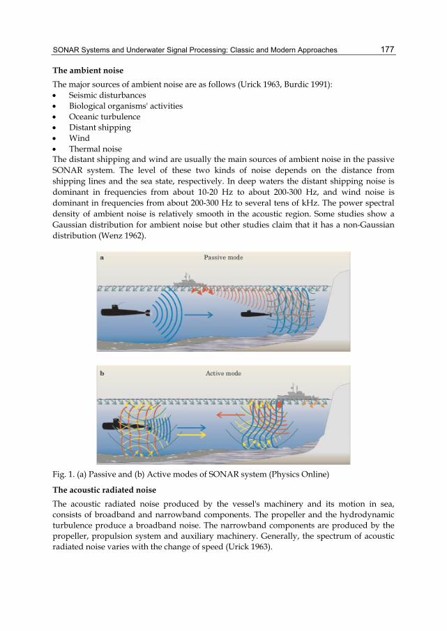
2.1. Basic Concepts SONAR systems are divided into two main categories – active and passive. Passive SONAR system (figure 1: (a)) provides monitoring the undersea environment without sending energy through the water. On the other hand, active SONAR system can act same as RADAR using responses from signals sent towards targets. Underwater signals obtained from passive SONAR contain valuable clues for source identification even in high noisy environments. Attempts on detection/classification of acoustic signals based on spectral characteristics have met little success in early era of SONAR system development (Urick 1963). In addition, finding the rules to classify objects in underwater is more difficult than those for surface vessels. Understanding the nature and characteristics of ambient noise and the acoustic radiated noise of vessels is of great importance in selecting the discriminating features and the classification algorithms. Therefore, we present a brief explanation about sources of ambient and radiated noises and their spectral characteristics.


177

The ambient noise

The major sources of ambient noise are as follows (Urick 1963, Burdic 1991): Seismic disturbances Biological organisms' activities Oceanic turbulence Distant shipping Wind Thermal noise The distant shipping and wind are usually the main sources of ambient noise in the passive SONAR system. The level of these two kinds of noise depends on the distance from shipping lines and the sea state, respectively. In deep waters the distant shipping noise is dominant in frequencies from about 10-20 Hz to about 200-300 Hz, and wind noise is dominant in frequencies from about 200-300 Hz to several tens of kHz. The power spectral density of ambient noise is relatively smooth in the acoustic region. Some studies show a Gaussian distribution for ambient noise but other studies claim that it has a non-Gaussian distribution (Wenz 1962).

Fig. 1. (a) Passive and (b) Active modes of SONAR system (Physics Online)

The acoustic radiated noise

The acoustic radiated noise produced by the vessel's machinery and its motion in sea, consists of broadband and narrowband components. The propeller and the hydrodynamic turbulence produce a broadband noise. The narrowband components are produced by the propeller, propulsion system and auxiliary machinery. Generally, the spectrum of acoustic radiated noise varies with the change of speed (Urick 1963).

Sonar Systems

178

Indeed, two main reasons for making the research in this area, challenging back to the nature of acoustic radiated noises which have: Rapid changes of characteristics over the time in both frequency and time Variations in Signal to Noise ratio (SNR) due to multipath propagation

2.2 Hidden markov model The Hidden Markov Model (HMM) approach to classify the SONAR signals is a promising technique, which has proven capability of detection/classification as well as applications in speech recognition (Rabiner 1989). In fact, the HMM is a stochastic model for speech applications as classifier of spoken words. Most current speech recognition algorithms are mainly based on HMM. In these models, speech signals are modeled as sequences of states with probabilities assigned to state transitions. Probability densities are associated with the observation of acoustic parameters. These parameters are considered from spectra or cepstra corresponding to the states or state transitions. The states are identified with the phonemes. A left-to-right HMM topology is mainly used for speech recognition. Nevertheless, a fully connected HMM topology which the transition from any state to other states is possible, can be more useful in our application of SONAR signal detection/classification. The left-to-right topology of HMM is known as Bakis model and the fully connected topology is known as Ergodic, as well. Exploiting the HMM approach to classify the signals consists of two main problems: Feature extraction of signals for training the models Preparing each model with training to classify the signals

Feature extraction

AR and cepstral coefficients are sensitive to the SNR of signals but the spectra components are more robust to variation of signals over time. However, AR model parameters can be used in stationery conditions, or even in short period SONAR signal processing. Therefore, they are preferred spectral features as input data to train the models. Using the spectra features, derived algorithms based on HMM are often robust. For an example, a typical spectrum of a diesel submarine noise is illustrated in figure 2.

Fig. 2. A typical spectrum of a diesel submarine


179

Though the SONAR signal received from such targets may be varied in time with respect to their SNR, interferences or even reverberation, but the spectrum features are mainly remained unchanged in which they can be used as main input data for training of HMM models. However, in severe conditions of ambient noise, detecting the main features is not so easy and may produce wrong amplitude or positions of main features.

HMM Training

Considering a first order, N-state Markov model (Rabiner 1989) in which state sequence Q is a realization of Markov model with probability:

(1)

where;

(2)

As a property of HMM, states of model cannot be directly observed, but can be estimated through a sequence of observations. In our purpose, it should be considered observations with continuous probability density. Thereafter, observation density vector will be:

(3)

where; specifies an HMM, completely.

By a number of observations of SONAR signals, we are able to train an HMM as optimal model. A density function of O is given by:

(4)

By using above formula we can compute density function of any observation and discriminate among related classes. The procedure of above-mentioned description is: Given a set of acoustic training data that is phonetically labeled (possibly with errors);

train an estimator to generate the data density for any hypothesized state: i.e. train an estimator for the emission probability density.

Given a probability estimator for the data likelihood of each state, use the dynamic programming to find the most likely sequence through the states in all possible sequences. This step is sometimes called forced Viterbi algorithm (Viterbi 1967).

Sonar Systems

180

The latter procedure can be proved that converges to a local optimum, however, in practice the stopping criterion can be modified by a threshold level. Thereafter, when an O of unknown class is given, we compute:

(5)

where; p* is optimal model and Q* is optimal state sequence and we can classify the source signal as belonging to the class p*. For instance, we considered simulated data of SONAR and applied previously mentioned model to evaluate the capability of HMM in detection/classification of SONAR signals. However, lack of real data has prevented to evaluate the different models. We considered two classes of submarines and simulated their noises. Figure 3 illustrates two examples of related spectra. We used feature vectors extracted from spectra for training two HMMs, nevertheless above vectors might be noisy in real SONAR systems. As simulation stage, we produced data with different SNR ranged from -20dB to 20dB in order to check robustness of algorithm. Therefore, we had at least two HMMs with optimal number of states.

(a) (b)

Fig. 3. Two spectra of simulated noises in frequency band of [10Hz, 1000Hz]: (a) Spectrum of simulated data in class#1, (b) Spectrum of simulated data in class#2

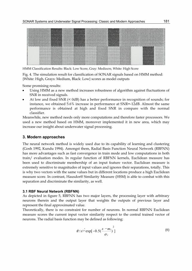
Now, for evaluation of method we consider another set of simulated data in order to provide test data. This procedure is iteratively continued until statistical results are provided. These statistical results are shown in figure 4. In this figure, all 24 results of classification scores have been graphically illustrated. The scores have been converted to grayscales, i.e., bright color means high score of classification. As shown in this figure, the class two has higher scores (brighter parts) then, as per majority vote to make a decision for received data over time, class #2 will be selected. In the first image, we considered simulated data from class #1. After preparing model (both stages of training test have been completed), a procedure similar to the test stage (named: evaluation stage) is iterated for 12 times. Therefore, we have 24 probability scores, which have been finally produced by two HMMs. The argument of the highest score determines class of input data.


181

HMM Classification Results: Black: Low Score, Gray: Mediocre, White: High Score

Fig. 4. The simulation result for classification of SONAR signals based on HMM method: {White: High, Grays: Medium, Black: Low} scores as model outputs

Some promising results: Using HMM as a new method increases robustness of algorithm against fluctuations of

SNR in received signals. At low and fixed SNR (< 0dB) has a better performance in recognition of sounds; for

instance, we obtained 5.6% increase in performance at SNR=-12dB. Almost the same performance is obtained at high and fixed SNR in compare with the normal classifier.

Meanwhile, new method needs only more computations and therefore faster processors. We used a new method based on HMM, moreover implemented it in new area, which may increase our insight about underwater signal processing.

3. Modern approaches

The neural network method is widely used due to its capability of learning and clustering (Gosh 1992, Kundu 1994). Amongst them, Radial Basis Function Neural Network (RBFNN) has more advantages such as fast convergence in train mode and low computations in both train/ evaluation modes. In regular function of RBFNN kernels, Euclidean measure has been used to discriminate membership of an input feature vector. Euclidean measure is extremely sensitive to magnitudes of input values and ignores their separations, totally. This is why two vectors with the same values but in different locations produce a high Euclidean measure score. In contrast, Hausdorff Similarity Measure (HSM) is able to combat with this separation and discriminate the similarity, as well.

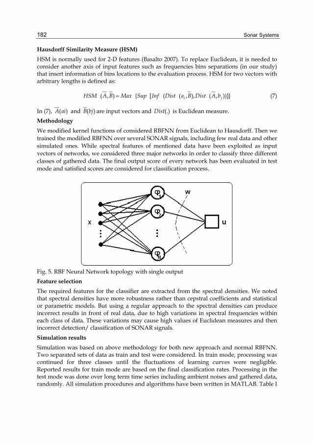
3.1 RBF Neural Network (RBFNN) As depicted in figure 5, RBFNN has two major layers, the processing layer with arbitrary neurons therein and the output layer that weights the outputs of previous layer and represent the final approximated value. Theoretically, there is no constraint for number of neurons. In normal RBFNN Euclidean measure scores the current input vector similarity respect to the central trained vector of neurons. The radial basis function may be defined as following:

])(5.0exp[

2)(

i

imxxi

(6)

Sonar Systems

182

Hausdorff Similarity Measure (HSM)

HSM is normally used for 2-D features (Basalto 2007). To replace Euclidean, it is needed to consider another axis of input features such as frequencies bins separations (in our study) that insert information of bins locations to the evaluation process. HSM for two vectors with arbitrary lengths is defined as:

( , ) { [ ( ( , ), ( , ))]}i jHSM A B Max Sup Inf Dist a B Dist A b (7)

In (7), ( )A ai and ( )B bj are input vectors and (.)Dist is Euclidean measure.

Methodology

We modified kernel functions of considered RBFNN from Euclidean to Hausdorff. Then we trained the modified RBFNN over several SONAR signals, including few real data and other simulated ones. While spectral features of mentioned data have been exploited as input vectors of networks, we considered three major networks in order to classify three different classes of gathered data. The final output score of every network has been evaluated in test mode and satisfied scores are considered for classification process.

Fig. 5. RBF Neural Network topology with single output

Feature selection

The required features for the classifier are extracted from the spectral densities. We noted that spectral densities have more robustness rather than cepstral coefficients and statistical or parametric models. But using a regular approach to the spectral densities can produce incorrect results in front of real data, due to high variations in spectral frequencies within each class of data. These variations may cause high values of Euclidean measures and then incorrect detection/ classification of SONAR signals.

Simulation results

Simulation was based on above methodology for both new approach and normal RBFNN. Two separated sets of data as train and test were considered. In train mode, processing was continued for three classes until the fluctuations of learning curves were negligible. Reported results for train mode are based on the final classification rates. Processing in the test mode was done over long term time series including ambient noises and gathered data, randomly. All simulation procedures and algorithms have been written in MATLAB. Table I


183

represents a comparison result between two RBFNN classifier with normal and modified kernels in both train/ test modes.

Method RBFNN (NORMAL)

RBFNN (HSM)

Class No. TRAIN (%) TEST (%) TRAIN

(%) TEST

(%) #1 93 87.4 95 92.5

#2 90 83.6 93 90.4 #3 88 74.0 88 83.7

Table 1. Classification Results

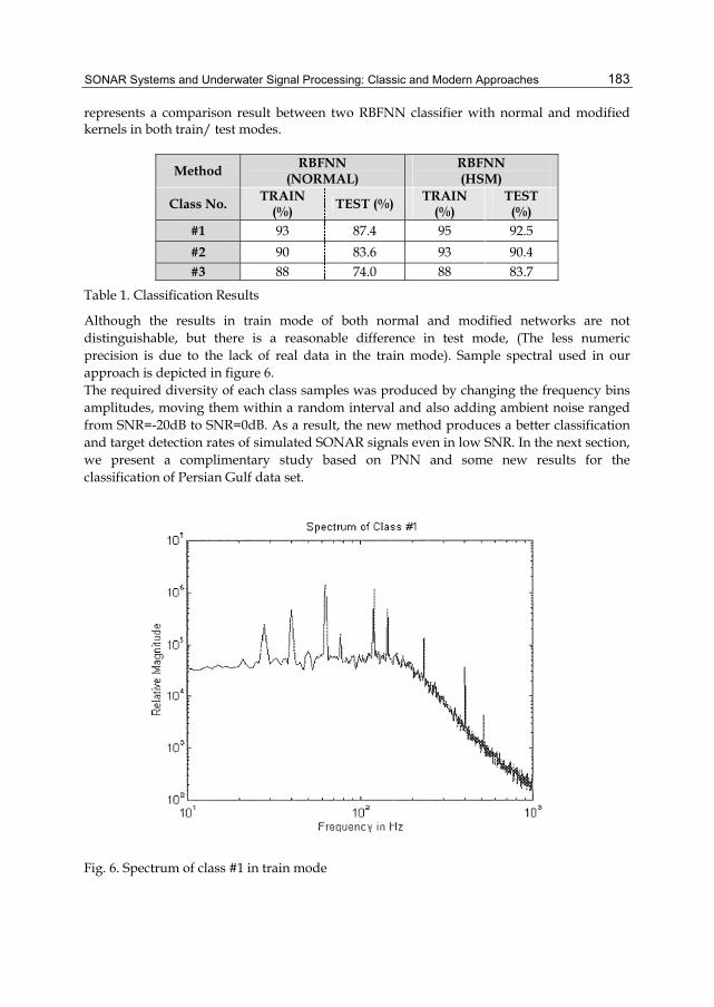
Although the results in train mode of both normal and modified networks are not distinguishable, but there is a reasonable difference in test mode, (The less numeric precision is due to the lack of real data in the train mode). Sample spectral used in our approach is depicted in figure 6. The required diversity of each class samples was produced by changing the frequency bins amplitudes, moving them within a random interval and also adding ambient noise ranged from SNR=-20dB to SNR=0dB. As a result, the new method produces a better classification and target detection rates of simulated SONAR signals even in low SNR. In the next section, we present a complimentary study based on PNN and some new results for the classification of Persian Gulf data set.

Fig. 6. Spectrum of class #1 in train mode

Sonar Systems

184

3.2 Probabilistic Neural Network (PNN) There are three layers in a PNN structure including: input, hidden and output layers. The length of feature vectors determines dimension of input layer. If we use d discriminating features for classification, the input layer dimension will be d. The hidden and the output layers consist of n patterns and c classes, respectively. Number of patterns n is chosen such that the convergence is guaranteed. Each pattern is d-dimensional and the output of the PNN is chosen from the set of classes 1 2, ,..., c . PNN is based on the Bayes decision rule, i.e. a trained PNN will decide i if:

( | ) ( ) ( | ) ( ) ; 1,..., i i j jp P p P j c and j i x x (8)

Where, 1 2{ , , ... , }dx x xx is the 1 d feature vector, and ( | )ip x and ( )iP are the d-dimensional conditional Probability Density Function (PDF) and prior probability obtained from the training data for i-th class, respectively. ( )iP is estimated by:

( ) ; 1,... , i

number of training data for i'th classP i c

total number of training data (9)

( | )ip x is estimated using Parzen windows. The Parzen (or Kernel) method is a non-parametric approach for PDF estimation. In this method, a symmetric d-dimensional window, which is usually a Gaussian window, is centered on each training sample. The windows corresponding to i-th class are superposed and appropriately normalized to give (x| )ip . The normalization is such that:

1... (x| ) ... 1 i dp dx dx

(10)

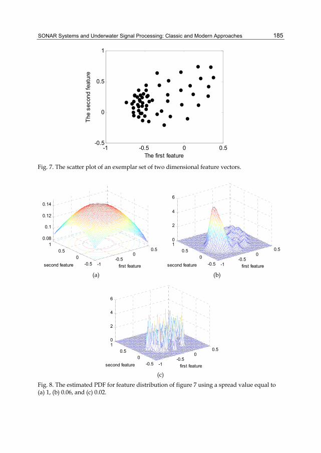
The conventional PNN needs an input parameter which is called the spread parameter. This parameter must be chosen by the user. The standard deviation of the Gaussian Parzen window is proportional to the spread parameter and it is identical for all samples in all classes. The most important disadvantage of the conventional PNN is the difficulty in selecting an appropriate spread value. The classification performance depends significantly on selecting an appropriate spread value. Too small spread values give very spiky PDF's and, too large spread values smooth out the details. To show this disadvantage of conventional PNN, consider a distribution of two dimensional feature vectors as shown in figure 7. The estimated PDF for set of points shown in figure 7 will be different for different values of spread parameter (the standard deviation of Gaussian windows). For example, using 1, 0.06 and 0.02 as values of the spread parameter, the estimated PDFs will be as shown in figures 8(a)-8(c), respectively. Although there are some approaches such as cross-validation for estimating an appropriate spread value, but they need a large number of data and high processing time. Thus, we determined the spread parameter by the trail and error. Another disadvantage of the conventional PNN is using the same spread parameter for all classes, which decreases the degree of freedom of the PDF estimator.


185

-1 -0.5 0 0.5-0.5

0

0.5

1

The first feature

The

sec

ond

feat

ure

Fig. 7. The scatter plot of an exemplar set of two dimensional feature vectors.

-1-0.5

00.5

-0.50

0.51

0.08

0.1

0.12

0.14

first featuresecond feature

-1-0.5

00.5

-0.5

00.5

10

2

4

6


(a) (b)

-1-0.5

00.5

-0.50

0.510

2

4

6


(c)

Fig. 8. The estimated PDF for feature distribution of figure 7 using a spread value equal to (a) 1, (b) 0.06, and (c) 0.02.

Sonar Systems

186

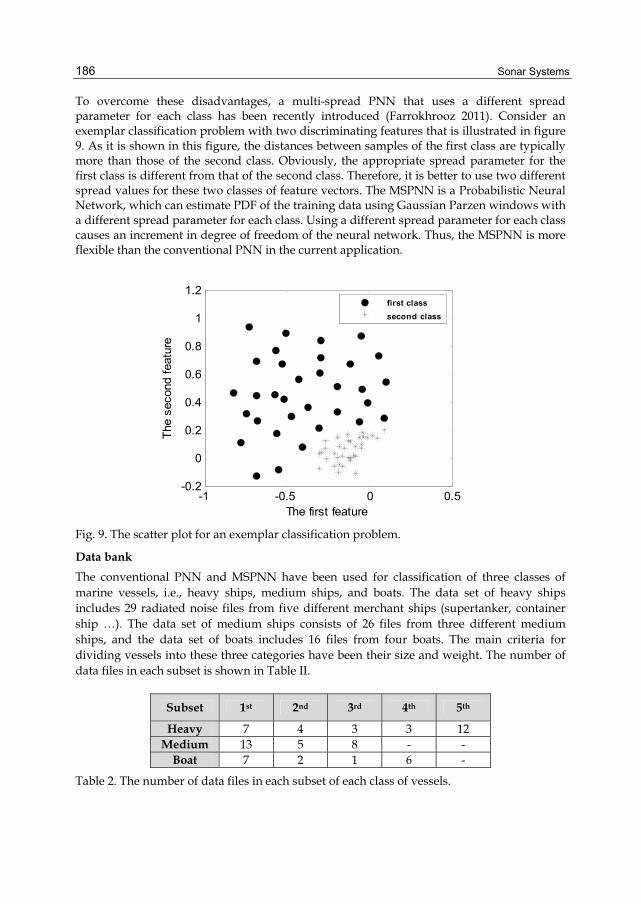
To overcome these disadvantages, a multi-spread PNN that uses a different spread parameter for each class has been recently introduced (Farrokhrooz 2011). Consider an exemplar classification problem with two discriminating features that is illustrated in figure 9. As it is shown in this figure, the distances between samples of the first class are typically more than those of the second class. Obviously, the appropriate spread parameter for the first class is different from that of the second class. Therefore, it is better to use two different spread values for these two classes of feature vectors. The MSPNN is a Probabilistic Neural Network, which can estimate PDF of the training data using Gaussian Parzen windows with a different spread parameter for each class. Using a different spread parameter for each class causes an increment in degree of freedom of the neural network. Thus, the MSPNN is more flexible than the conventional PNN in the current application.

-1 -0.5 0 0.5-0.2

0

0.2

0.4

0.6

0.8

1

1.2

The first feature

The

sec

ond

feat

ure

first class

second class

Fig. 9. The scatter plot for an exemplar classification problem.

Data bank

The conventional PNN and MSPNN have been used for classification of three classes of marine vessels, i.e., heavy ships, medium ships, and boats. The data set of heavy ships includes 29 radiated noise files from five different merchant ships (supertanker, container ship …). The data set of medium ships consists of 26 files from three different medium ships, and the data set of boats includes 16 files from four boats. The main criteria for dividing vessels into these three categories have been their size and weight. The number of data files in each subset is shown in Table II.

Subset 1st 2nd 3rd 4th 5th

Heavy 7 4 3 3 12 Medium 13 5 8 - -

Boat 7 2 1 6 -

Table 2. The number of data files in each subset of each class of vessels.


187

Each subset of files corresponds to one vessel. All files have been recorded in the Persian Gulf at low sea states. The time length of each file is five seconds and the recording sampling frequency equals 2560 samples/second. All data files have contents only in the 125-500Hz frequency band.

Feature selection

The set of selected features for classifying the radiated noises of ships can be divided into two categories: the features extracted from AR model of signals and the features directly extracted from the estimated PSD of signals. The first category contains the coefficients of AR model of signals with AR order 15 or 13, and the poles of AR model with order 2. The second category of discriminating features includes 6 features directly extracted from PSD of signals.

Performance evaluation

In this section, we evaluate the classification performance of conventional PNN and MSPNN with the method in (Farrokhrooz 2011) for spread estimation by applying them to the bank of real acoustic radiated noises of marine vessels. We define the performance of a classifier for a class as the probability of correct decision for the data of that class. In order to evaluate the performance of the classifiers, we divided the data bank into two parts, the training data set and the test data set. After feature extraction, the extracted features of training data set are used for classifier training and the features of test data set are used for evaluating the performance of the classifier. We used a training data set as introduced in Table III. In each of the performance evaluations in this section, this data set of Table III is used for training and the rest of data bank files are used as the test data set. In each performance evaluation, the performance of conventional PNN will be shown versus spread parameter values and the performance of MSPNN will be demonstrated versus the multiplier x.

Subset used for training

heavy ship file medium ship

file boat file

Training data set

7 randomly selected files

from all subsets


from all subsets


from all subsets

Table 3. The number of data files in each subset of each class of vessels

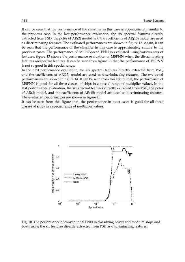
In this subsection the performance of conventional PNN is evaluated using various sets of features. Figure 10 shows the performance evaluation of conventional PNN when the discriminating features are spectral features. As shown in this figure, selecting a proper spread value causes high probability of correct decision for heavy and medium ships. However, the probability of correct decision for boats is not high in these cases. In the next performance evaluation, the six spectral features directly extracted from PSD, and the coefficients of AR(15) model are used as discriminating features. The evaluated performances are shown in figure 11.

Sonar Systems

188

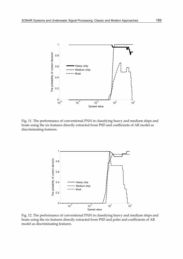
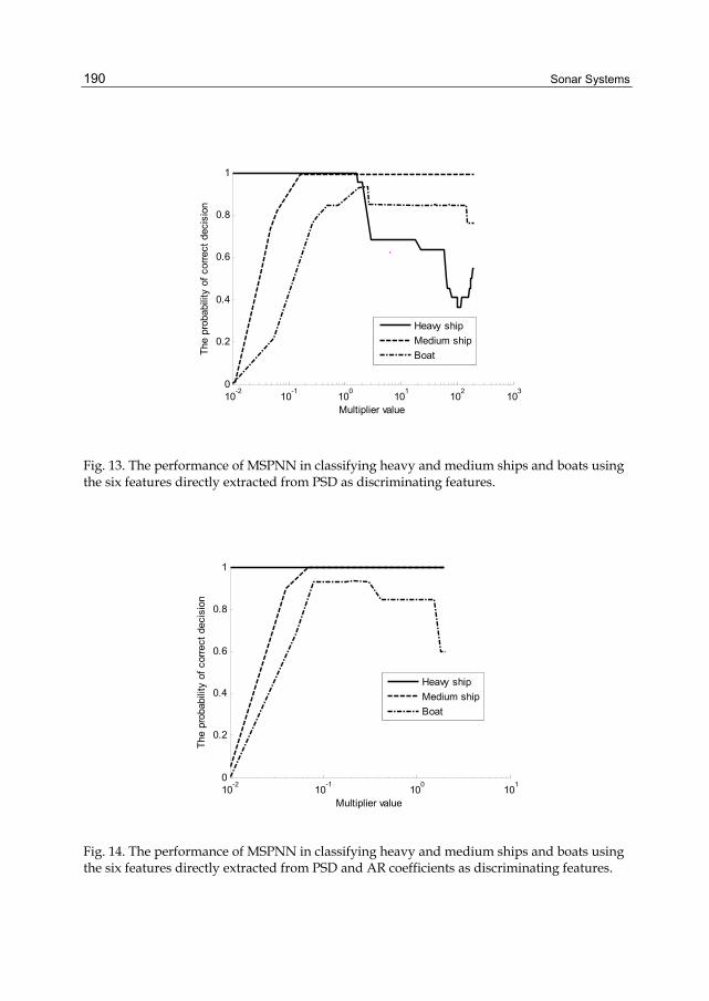
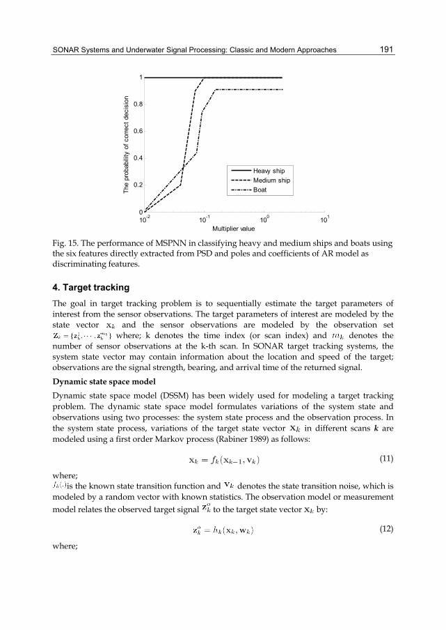
It can be seen that the performance of the classifier in this case is approximately similar to the previous case. In the last performance evaluation, the six spectral features directly extracted from PSD, the poles of AR(2) model, and the coefficients of AR(15) model are used as discriminating features. The evaluated performances are shown in figure 12. Again, it can be seen that the performance of the classifier in this case is approximately similar to the previous cases. The performance of Multi-Spread PNN is evaluated using various sets of features. figure 13 shows the performance evaluation of MSPNN when the discriminating features arespectral features. It can be seen from figure 13 that the performance of MSPNN is not so good in this special range. In the next performance evaluation, the six spectral features directly extracted from PSD, and the coefficients of AR(15) model are used as discriminating features. The evaluated performances are shown in figure 14. It can be seen from this figure that, the performance of MSPNN is good for all three classes of ships in a special range of multiplier values. In the last performance evaluation, the six spectral features directly extracted from PSD, the poles of AR(2) model, and the coefficients of AR(15) model are used as discriminating features. The evaluated performances are shown in figure 15. It can be seen from this figure that, the performance in most cases is good for all three classes of ships in a special range of multiplier values.

10-6

10-4

10-2

100

102

0

0.2

0.4

0.6

0.8

1

Spread value

The

pro

babi

lity

of c

orre

ct d

ecis

ion

Heavy ship

Medium ship

Boat

Fig. 10. The performance of conventional PNN in classifying heavy and medium ships and boats using the six features directly extracted from PSD as discriminating features.


189

10-6

10-4

10-2

100

102

0

0.2

0.4

0.6

0.8

1

Spread value

The

pro

babi

lity

of c

orre

ct d

ecis

ion

Heavy ship

Medium ship

Boat

Fig. 11. The performance of conventional PNN in classifying heavy and medium ships and boats using the six features directly extracted from PSD and coefficients of AR model as discriminating features.

10-4

10-2

100

102

0

0.2

0.4

0.6

0.8

1

Spread value

The

pro

babi

lity

of c

orre

ct d

ecis

ion

Heavy ship

Medium shipBoat

Fig. 12. The performance of conventional PNN in classifying heavy and medium ships and boats using the six features directly extracted from PSD and poles and coefficients of AR model as discriminating features.

Sonar Systems

190

10-2

10-1

100

101

102

103

0

0.2

0.4

0.6

0.8

1

Multiplier value

The

pro

babi

lity

of c

orre

ct d

ecis

ion

Heavy ship

Medium ship

Boat

Fig. 13. The performance of MSPNN in classifying heavy and medium ships and boats using the six features directly extracted from PSD as discriminating features.

10-2

10-1

100

101

0

0.2

0.4

0.6

0.8

1

Multiplier value

The

pro

babi

lity

of c

orre

ct d

ecis

ion

Heavy ship

Medium ship

Boat

Fig. 14. The performance of MSPNN in classifying heavy and medium ships and boats using the six features directly extracted from PSD and AR coefficients as discriminating features.


191

10-2

10-1

100

101

0

0.2

0.4

0.6

0.8

1

Multiplier value

The

pro

babi

lity

of c

orre

ct d

ecis

ion

Heavy ship

Medium ship

Boat

Fig. 15. The performance of MSPNN in classifying heavy and medium ships and boats using the six features directly extracted from PSD and poles and coefficients of AR model as discriminating features.

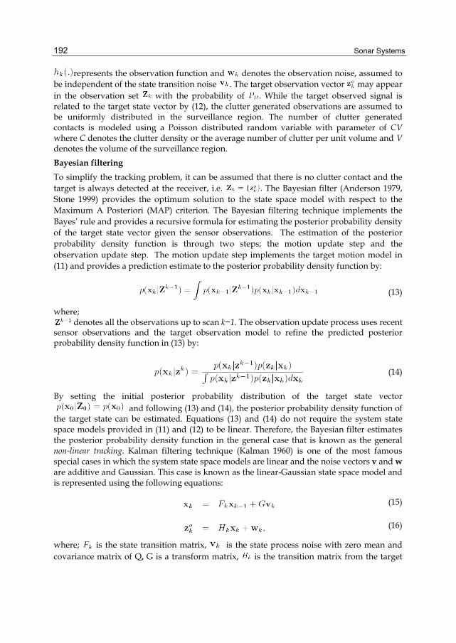
4. Target tracking

The goal in target tracking problem is to sequentially estimate the target parameters of interest from the sensor observations. The target parameters of interest are modeled by the state vector and the sensor observations are modeled by the observation set

where; k denotes the time index (or scan index) and denotes the number of sensor observations at the k-th scan. In SONAR target tracking systems, the system state vector may contain information about the location and speed of the target; observations are the signal strength, bearing, and arrival time of the returned signal.

Dynamic state space model

Dynamic state space model (DSSM) has been widely used for modeling a target tracking problem. The dynamic state space model formulates variations of the system state and observations using two processes: the system state process and the observation process. In the system state process, variations of the target state vector in different scans k are modeled using a first order Markov process (Rabiner 1989) as follows:

(11)

where; is the known state transition function and denotes the state transition noise, which is

modeled by a random vector with known statistics. The observation model or measurement model relates the observed target signal to the target state vector by:

(12)

where;

Sonar Systems

192

represents the observation function and denotes the observation noise, assumed to be independent of the state transition noise . The target observation vector may appear in the observation set with the probability of . While the target observed signal is related to the target state vector by (12), the clutter generated observations are assumed to be uniformly distributed in the surveillance region. The number of clutter generated contacts is modeled using a Poisson distributed random variable with parameter of CV where C denotes the clutter density or the average number of clutter per unit volume and V denotes the volume of the surveillance region.

Bayesian filtering

To simplify the tracking problem, it can be assumed that there is no clutter contact and the target is always detected at the receiver, i.e. . The Bayesian filter (Anderson 1979, Stone 1999) provides the optimum solution to the state space model with respect to the Maximum A Posteriori (MAP) criterion. The Bayesian filtering technique implements the Bayes’ rule and provides a recursive formula for estimating the posterior probability density of the target state vector given the sensor observations. The estimation of the posterior probability density function is through two steps; the motion update step and the observation update step. The motion update step implements the target motion model in (11) and provides a prediction estimate to the posterior probability density function by:

(13)

where; denotes all the observations up to scan k−1. The observation update process uses recent

sensor observations and the target observation model to refine the predicted posterior probability density function in (13) by:

(14)

By setting the initial posterior probability distribution of the target state vector and following (13) and (14), the posterior probability density function of

the target state can be estimated. Equations (13) and (14) do not require the system state space models provided in (11) and (12) to be linear. Therefore, the Bayesian filter estimates the posterior probability density function in the general case that is known as the general non-linear tracking. Kalman filtering technique (Kalman 1960) is one of the most famous special cases in which the system state space models are linear and the noise vectors v and w are additive and Gaussian. This case is known as the linear-Gaussian state space model and is represented using the following equations:

(15)

(16)

where; is the state transition matrix, is the state process noise with zero mean and covariance matrix of Q, G is a transform matrix, is the transition matrix from the target


193

state space to the observation space, and is the Gaussian additive observation noise with zero mean and covariance matrix of R. Using the linear-Gaussian model, the target state vector is the linear combination of the Gaussian distributed vector v then is Gaussian. This is the Key assumption in deriving the Kalman filter equations. The estimation of the target state vector, denoted by is computed as follows:

(17)

(18)

(19)

(20)

where;

(21)

is the covariance matrix of and,

(22)

is known as the Kalman gain. The Kalman filter provides the expected value and the covariance matrix of the posterior probability density function . In a linear-Gaussian state space model, Kalman filter is the optimum solution in the senses of the Minimum Mean Square Error (MMSE), Maximum Likelihood (ML), and Maximum A Posteriori (MAP) criteria (Anderson 1979, Kalman 1960). Because of the efficiency and simple implementation of the Kalman filter, many approaches have been developed that focus on linearization of state space model and applying Kalman filtering to the linear model. The most popular approach in this group is the well known extended Kalman filter (EKF) (Bar-Shalom 1988, Kailath 2000) which makes the state space model linear using Taylor series expansions of the nonlinear functions. While the EKF performs well under mild nonlinearity, it suffers from performance loss under sever nonlinearities. Another approach to linearization of state space model, presented in (Norgaard 2000), implements the polynomial approximation of a nonlinear function. This technique, known in the literatures as the central-difference Kalman filter (CDKF), can replace the EKF in some practical applications in which linearization using Taylor series is not so accurate. For both EKF and CDKF techniques, there is an implicit Gaussian prior assumption on the posterior density function due to applying the Kalman filter. Another group of proposed techniques assumes an explicit prior form (normally Gaussian) for the posterior density function. Perhaps the most famous approach in this group is the unscented Kalman filter (UKF) (Julier 2000, Julier 2004) which uses a novel nonlinear transformation of the mean and covariance matrices. In this approach, the mean and covariance matrices of the assumed Gaussian posterior density are parameterized by a set of samples, and these samples are updated through processing by a nonlinear filter. In the Quadrature Kalman filter (QKF) (Ito 2000, Arasaratnam 2007) the assumed Gaussian posterior density is parameterized through

Sonar Systems

194

a set of Gauss-Hermite quadrature points, and the nonlinear process and observation functions are linear using statistical linear regression (SLR). The Cubature Kalman Filter (CKF) (Cubature 2009) uses a spherical-radial cubature rule for numerical computation of the multivariate moment integrals that appear in the Bayesian filter formulation. The Gaussian posterior density function is the key assumption in this numerical computation. Some existing approaches do not have explicit assumptions on the posterior distribution. Instead, they estimated a discrete set of parameters and used them to approximate the posterior density function. The Gaussian mixture filter (Alspach 1972), for example, estimates a set of discrete weight parameters and implements these weights to approximate the posterior density function using a weighted sum of Gaussian density functions. It is shown in (Sorenson 1971) that any practical density function can be represented by a weighted sum of Gaussian density functions and as the number of Gaussian densities increases, the approximation will converge uniformly to the desired density function. Recently, particle filtering (PF) (Djuric 2003) has become popular in many applications of statistical signal processing. In particle filtering, a desired posterior density function is estimated through a set of particles and associated weights. At each time update, new particles are generated via sampling from an importance function, and the weight associated with each particle is updated. With fast development of powerful computational systems, the numerical approach to solve the Bayesian inference equation that was first introduced in (Bucy 1971) has renewed its attraction through the point mass approach (Simandl 2006). In the point mass approach, a regular grid discretizes the system state, and the Bayesian filter is evaluated numerically on the discrete points. The tree search target tracking technique, introduced in (Nelson 2009, Roufarshbaf 2009) approximates the Bayesian filtering recursions by generating a tree of possible target state variations and finding the solution by navigating the search tree using the Stack algorithm.

Data association techniques

Thus far, we assumed that there are no clutter observations at the receiver and the target is detected in each scan. When clutter observations appear at the receiver, the above techniques cannot be performed directly for tracking the target and the observation contacts must be associated to either the target(s) or clutter. In this section, we discuss the most famous techniques for data association. We also consider the cases in which the target contact is not detected at the receiver. The early work on target tracking that addresses the challenge of data association was introduced in (Sittler 1964). The approach splits a track whenever more than one measurement is present. Then it calculates the likelihood function for each track and the tracks with likelihoods less than a predefined threshold are deleted. In the nearest neighbor Kalman filter (NNKF) approach (Singer 1971, Sea 1971, Singer 1973), the contact that has the smallest statistical distance to the predicted target track is considered as a true target observation and the others are considered as clutter. The probabilistic data association filter (PDAF) introduced in (Bar-Shalom 1975), provides a suboptimal Bayesian approach for data association in the single target tracking problem. In this approach, the target track is updated using the weighted sum of all possible track updates from each data association hypothesis of the current scan. When a single target is present, the optimal Bayesian approach for data association considers all possible association hypotheses from the target initiation time index to the current time and updates the target track using sum of the all possible track updates weighted by evaluated


195

association probabilities (Bar-Shalom 1988). Since the optimal Bayesian method is computationally intractable, suboptimal approaches have been suggested. The joint probabilistic data association filter (JPDAF) (Fortmann 1983) is an extension to the PDAF algorithm for multiple target tracking. In this approach, all possible association hypotheses of the current time are evaluated for all targets, and the tracks are updated by a weighted sum of all possible track updates from the data association hypotheses. Other data association algorithms implements either MAP or ML approaches to find the best sequence of measurements that can be associated to each target. The Viterbi algorithm (Viterbi 1967, Wolf 1989) and the Expectation Maximization (EM) algorithm (Gauvrit 1997) have been widely used for this purposed. Multi-hypothesis tracking (MHT) (Blackman 2004) is a MAP estimator in which at each scan, instead of combining the hypotheses like JPDAF or selecting the best hypothesis like nearest neighbor (NN), the algorithm makes a tree of possible association hypotheses and decides based on the future observations through a MAP estimator. All of the data association approaches discussed above is combined with a tracking technique such as EKF, to estimate the target track within the clutter observations. As an example, we discuss the details of the PDAF algorithm which is one of the most common approaches in SONAR target tracking. In the PDAF technique, the data association probabilities and j = are defined for each scan as the probability that the jth observation of the scan is generated by the target and others are related to the clutter. The special case is defined as the probability that all the observations are generated by clutter and the target generated observation is not detected. Using the data association probabilities in the Kalman filter, it is sufficient to change the equations (19) and (20) as follows:

(23)

(24)

where;

(25)

(26)

(27)

The association probabilities have been calculated in literatures and the results are as following:

(28)

(29)

Sonar Systems

196

where;

(30)

and M denotes the dimension of the observation vector .

Recent techniques

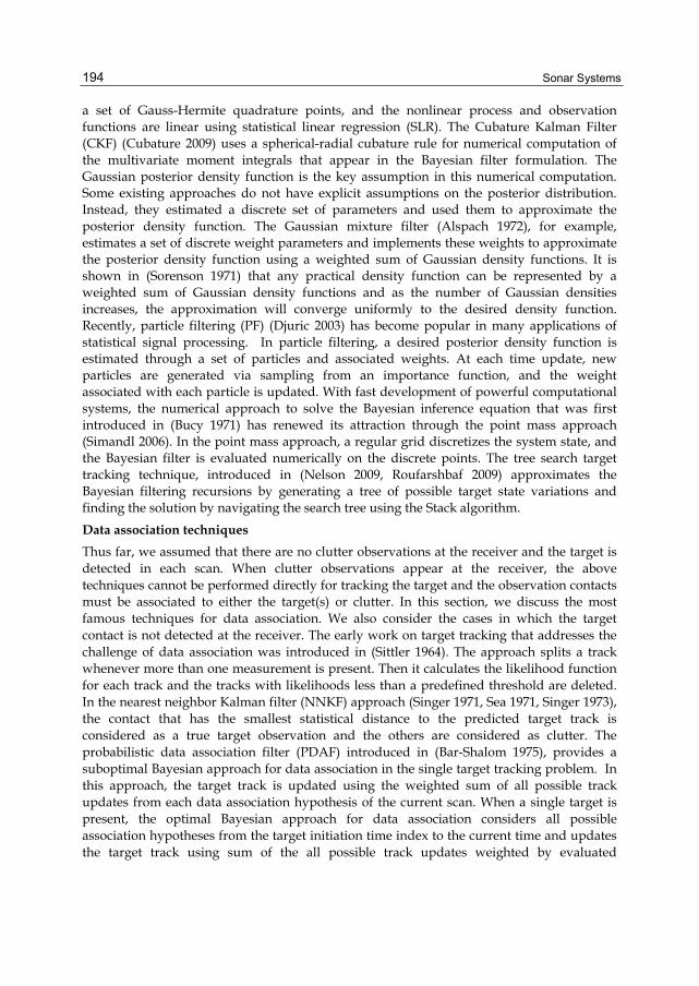
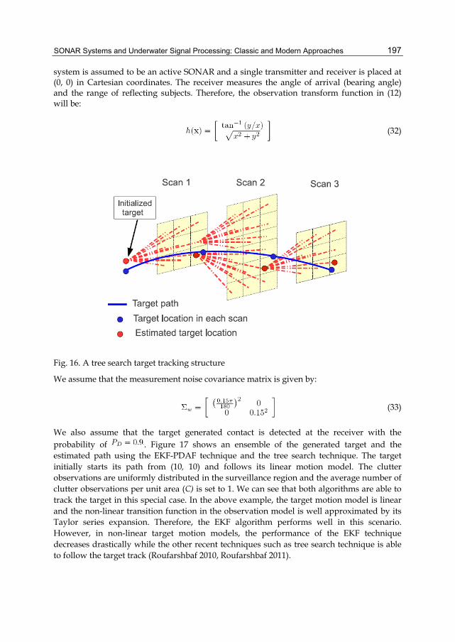
Some recent techniques in target tracking including sequential Monte Carlo techniques and the tree search techniques combine the data association problem and the target tracking problem as a unified problem. Sequential Monte Carlo approaches (Hue 2002) have been introduced in target tracking problems for both track estimation and data association. In the approach presented in (Hue 2002), Gibbs sampling is implemented to solve the data association problem, and particle filtering is used for target track estimation. The algorithm is developed for the cases of single target, multiple targets, single receiver, and multiple receiver systems for both fixed and variable number of targets (Hue 2002, Arulampalam 2002). Recently the stack-based tree search algorithm (Roufarshbaf 2011, Nelson 2009, Roufarshbaf 2009), has been developed for tracking the targets in non-linear environments with high clutter density. The approach is classified as a sub-optimum Bayesian approach for both track estimation and data association and is implemented for linear/non-linear state space models as well as Gaussian/non-Gaussian additive noise. The stack algorithm was originally developed as a sequential method for decoding error-correcting convolutional codes in digital communications (Jelinek 1969). It has more recently been suggested as a lower-complexity alternative to trellis-based techniques, e.g. the Viterbi algorithm (Viterbi 1967), for ML sequence detection of data transmitted over a dispersive channel (Xiong 1990, Nelson 2006). In target tracking applications, the stack algorithm navigates a tree in search of the target path with the largest likelihood, or metric. A set of possible paths and their associated metrics are stored in a list (or stack), and at each iteration, the algorithm extends the path with the largest metric. A simple example of the stack algorithm for target tracking is given in figure 16. The algorithm starts from an initial target estimate and makes a search tree of possible target movements from its currently approximated locations. At the end of the observation, the target path that has the highest probability among the extended paths of the search tree is selected as the estimated target track. As a single example, consider a target that follows a linear motion model. The target state vector is defined by , where; (x, y) denotes the position of the target in Cartesian coordinates, and (x˙, y˙) denotes the target velocity in Cartesian coordinates. The parameters of the target motion model (15) are set as follows:

(31)

where; is the time between scans. In this model, the state transition noise vector determines the acceleration (in the x and y directions) over the time interval and the covariance matrix of is set to where I denotes the identity matrix. The


197

system is assumed to be an active SONAR and a single transmitter and receiver is placed at (0, 0) in Cartesian coordinates. The receiver measures the angle of arrival (bearing angle) and the range of reflecting subjects. Therefore, the observation transform function in (12) will be:

(32)

Fig. 16. A tree search target tracking structure

We assume that the measurement noise covariance matrix is given by:

(33)

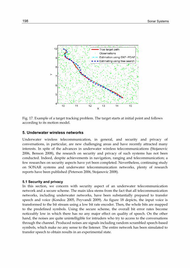
We also assume that the target generated contact is detected at the receiver with the probability of . Figure 17 shows an ensemble of the generated target and the estimated path using the EKF-PDAF technique and the tree search technique. The target initially starts its path from (10, 10) and follows its linear motion model. The clutter observations are uniformly distributed in the surveillance region and the average number of clutter observations per unit area (C) is set to 1. We can see that both algorithms are able to track the target in this special case. In the above example, the target motion model is linear and the non-linear transition function in the observation model is well approximated by its Taylor series expansion. Therefore, the EKF algorithm performs well in this scenario. However, in non-linear target motion models, the performance of the EKF technique decreases drastically while the other recent techniques such as tree search technique is able to follow the target track (Roufarshbaf 2010, Roufarshbaf 2011).

Sonar Systems

198

Fig. 17. Example of a target tracking problem. The target starts at initial point and follows according to its motion model.

5. Underwater wireless networks

Underwater wireless telecommunication, in general, and security and privacy of conversations, in particular, are new challenging areas and have recently attracted many interests. In spite of the advances in underwater wireless telecommunications (Stojanovic 2006, Benson 2008), the research on security and privacy of such systems has not been conducted. Indeed, despite achievements in navigation, ranging and telecommunication; a few researches on security aspects have yet been completed. Nevertheless, continuing study on SONAR systems and underwater telecommunication networks, plenty of research reports have been published (Peterson 2006, Stojanovic 2008).

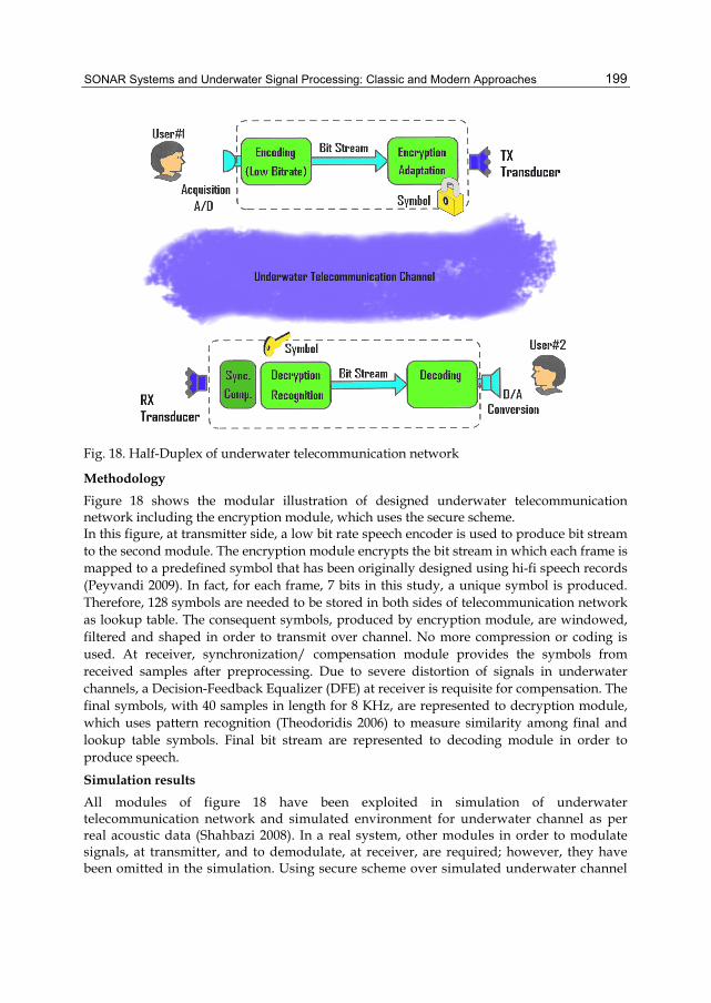
5.1 Security and privacy In this section, we concern with security aspect of an underwater telecommunication network and a secure scheme. The main idea stems from the fact that all telecommunication networks, including underwater networks, have been substantially prepared to transfer speech and voice (Kondoz 2005, Peyvandi 2009). As figure 18 depicts, the input voice is transformed to the bit stream using a low bit rate encoder. Then, the whole bits are mapped to the predefined symbols. Using the secure scheme, the overall bit error rates become noticeably low in which there has no any major effect on quality of speech. On the other hand, the noises are quite unintelligible for intruders who try to access to the conversations through the channel. Produced noises are signals including random scrambled speech-based symbols, which make no any sense to the listener. The entire network has been simulated to transfer speech to obtain results in an experimental state.


199

Fig. 18. Half-Duplex of underwater telecommunication network

Methodology

Figure 18 shows the modular illustration of designed underwater telecommunication network including the encryption module, which uses the secure scheme. In this figure, at transmitter side, a low bit rate speech encoder is used to produce bit stream to the second module. The encryption module encrypts the bit stream in which each frame is mapped to a predefined symbol that has been originally designed using hi-fi speech records (Peyvandi 2009). In fact, for each frame, 7 bits in this study, a unique symbol is produced. Therefore, 128 symbols are needed to be stored in both sides of telecommunication network as lookup table. The consequent symbols, produced by encryption module, are windowed, filtered and shaped in order to transmit over channel. No more compression or coding is used. At receiver, synchronization/ compensation module provides the symbols from received samples after preprocessing. Due to severe distortion of signals in underwater channels, a Decision-Feedback Equalizer (DFE) at receiver is requisite for compensation. The final symbols, with 40 samples in length for 8 KHz, are represented to decryption module, which uses pattern recognition (Theodoridis 2006) to measure similarity among final and lookup table symbols. Final bit stream are represented to decoding module in order to produce speech.

Simulation results

All modules of figure 18 have been exploited in simulation of underwater telecommunication network and simulated environment for underwater channel as per real acoustic data (Shahbazi 2008). In a real system, other modules in order to modulate signals, at transmitter, and to demodulate, at receiver, are required; however, they have been omitted in the simulation. Using secure scheme over simulated underwater channel

Sonar Systems

200

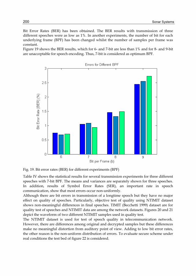
Bit Error Rates (BER) has been obtained. The BER results with transmission of three different speeches were as low as 1%. In another experiments, the number of bit for each underlying frame (BPF) has been changed whilst the number of samples per frame was constant. Figure 19 shows the BER results, which for 6- and 7-bit are less than 1% and for 8- and 9-bit are unacceptable for speech encoding. Thus, 7-bit is considered as optimum BPF.

Fig. 19. Bit error rates (BER) for different experiments (BPF)

Table IV shows the statistical results for several transmission experiments for three different speeches with 7-bit BPF. The means and variances are separately shown for three speeches. In addition, results of Symbol Error Rates (SER), an important rate in speech communication, show that most errors occur non-uniformly. Although there are bit errors in transmission of a longtime speech but they have no major effect on quality of speeches. Particularly, objective test of quality using NTIMIT dataset shows non-meaningful differences in final speeches. TIMIT (Becchetti 1999) dataset are for quality test of speeches and NTIMIT data are among the network datasets. Figures 20 and 21 depict the waveform of two different NTIMIT samples used in quality test. The NTIMIT dataset is used for test of speech quality in telecommunication network. However, there are differences among original and decrypted samples but these differences make no meaningful distortion from auditory point of view. Adding to low bit error rates, the other reason is the non-uniform distribution of errors. To evaluate secure scheme under real conditions the test bed of figure 22 is considered.


201

Exp. No. BER (%) SER (%)

Mean Variance Mean Variance

#1 0.96 0.05 0.55 0.09

#2 1.07 0.07 0.60 0.12

#3 0.93 0.06 0.52 0.10

Table 4. Simulation Results

Fig. 20. NTIMIT dataset sample I (a) Original (b) After decoding

Fig. 21. NTIMIT dataset sample II (a) Original (b) After decoding

Sonar Systems

202

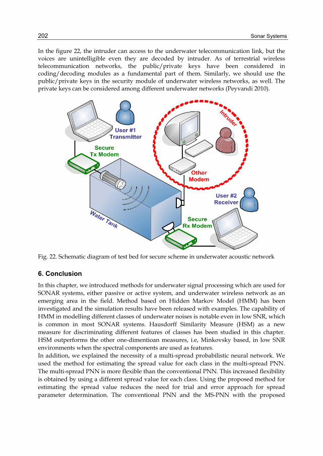
In the figure 22, the intruder can access to the underwater telecommunication link, but the voices are unintelligible even they are decoded by intruder. As of terrestrial wireless telecommunication networks, the public/private keys have been considered in coding/decoding modules as a fundamental part of them. Similarly, we should use the public/private keys in the security module of underwater wireless networks, as well. The private keys can be considered among different underwater networks (Peyvandi 2010).

Fig. 22. Schematic diagram of test bed for secure scheme in underwater acoustic network

6. Conclusion

In this chapter, we introduced methods for underwater signal processing which are used for SONAR systems, either passive or active system, and underwater wireless network as an emerging area in the field. Method based on Hidden Markov Model (HMM) has been investigated and the simulation results have been released with examples. The capability of HMM in modelling different classes of underwater noises is notable even in low SNR, which is common in most SONAR systems. Hausdorff Similarity Measure (HSM) as a new measure for discriminating different features of classes has been studied in this chapter. HSM outperforms the other one-dimentioan measures, i.e, Minkovsky based, in low SNR environments when the spectral components are used as features. In addition, we explained the necessity of a multi-spread probabilistic neural network. We used the method for estimating the spread value for each class in the multi-spread PNN. The multi-spread PNN is more flexible than the conventional PNN. This increased flexibility is obtained by using a different spread value for each class. Using the proposed method for estimating the spread value reduces the need for trial and error approach for spread parameter determination. The conventional PNN and the MS-PNN with the proposed


203

method for estimating the spread parameter were applied to the radiated ship noise classification problem. A bank of real radiated noise data were used to evaluate the performance of the conventional and MS-PNN. In all performance evaluations, which is used for conventional PNN as the classifier, selecting a proper spread value caused high probability of correct decision for heavy and medium ships. In all performance evaluations, which is used for the MS-PNN as the classifier, there is a relatively wide range of multipliers in which the best performance occurs. We also considered target tracking problem in sonar systems. A target tracking problem was modeled using the conventional DSSM. Then, we reviewed the classic Bayesian target tracking techniques and its closed form Kalman filtering approach that is optimum for linear-Gaussian models. Then, we studied tracking of low observable targets through clutter contacts and we reviewed the recent approaches in target tracking that are more efficient in non-linear scenarios. Through an example, we show how a classic EKF technique and a recent tree search technique are able to track a single target through clutter contacts. In the last section in this chapter, we have proposed a new scheme for providing secure conversation in underwater telecommunication systems. Although, there are bit errors in near all communications, low bit errors with non-uniform distribution have unintelligible effect on quality of speeches. The quality test has been provided using NTIMIT dataset samples. The results showed that the proposed scheme for underwater wireless telecommunication systems is reliable in an experimental state. The environmental test of proposed scheme is ongoing.

7. Acknowledgment

We would like to acknowledge people who have commented and made suggestions on this work. Without their help, there would be fewer results and the existing descriptions would be more difficult to read. In particular, we would like to express our thanks to Dr. M. Karimi for his valuable advices, Dr. A. Ebrahimi for discussion on early version of section 5, Dr. M. Dianati for helpful discussion and Mr A. Maleki, H. Kamalpour for their help to provide additional analysis in datasets. At finally yet importantly, the first author would like to thank Dr. Hassan Peyvandi for his support and help during tough time in the last year.

8. References

Abrahat, R. J.; Kneale, P. E & See, L. M. (2004). Neural Networks for Hydrological Modelling, A. A. Balkema Publishers, London.

Alspach, D. L. & Sorenson, H. W. (1972). “Nonlinear Bayesian estimation using Gaussian sum approximations," IEEE Trans. On Automatic Control, vol. 17, no. 4, pp. 439-448.

Anderson, B. D. O. & Moore, J. B. (1979). Optimal Filtering. Dover Publications. Arasaratnam, I. & Haykin, S. (2007). ”Discrete-time nonlinear filtering algorithms using

Gauss-Hermite quadrature," Proceedings of the IEEE, vol. 95, no. 5, pp. 953-977. Arasaratnam, I. & Haykin, S. (2009). “Cubature Kalman Filter (CKF)," IEEE Trans. on

Automatic Control, vol. 54, pp. 1254-1269. Arulampalam, S.; Maskell, S.; Gordon, N. & Clapp, T. (2002). “A tutorial on particle filters

for online non-linear/non- Gaussian Bayesian tracking," IEEE Trans. on Signal Processing, vol. 50, no. 2, pp. 174-188.

Sonar Systems

204

Bar-Shalom, Y. & Tse, E. (1975). “Tracking in a cluttered environment with probabilistic data association," Automatica, vol. 11, pp. 451-460.

Bar-Shalom, Y. & Fortmann, T. E. (1988). Tracking and Data Association. Academic Press, Inc. Basalto, N.; et al, (2007). “Hausdorff Clustering of Financial Time Series,” Physica A, 379, pp.

636-644. Becchetti, C. & Ricotti, L. P. (1999). Speech Recognition, John Wiley, ISBN: 0-471-97730-6. Blackman, S. (2004). ”Multiple hypothesis tracking for multiple target tracking," IEEE

Aerospace and Electronic Systems Magazine, vol. 19, no. 1, pp. 5-18. Jelinek,F. (1969), “Fast sequential decoding algorithm using a stack,” IBM journal of research

and development, vol. 13, no. 6, pp. 675–685 Bucy, R. & Senne, K. (1971). “Digital synthesis of nonlinear filters," Automatica, vol. 7, pp.

287-298. Burdic, W. S. (1991). Underwater Acoustic System Analysis, ISBN: 0139476075, Prentice-Hall,

2nd edition. Djuric, P. M.; Kotecha, J. H.; Zhang, J.; Huang, Y.; Ghirmai, T.; Bugallo, M. F. & Miguez, J.

(2003). “Particle filtering," IEEE Signal Processing Magazine, vol. 20, pp. 19-38. Duda, R. O.; Hart, P. E. & Stork, D. G. (2000). Pattern Classification, ISBN: 0471056693, John

Wiley & Sons, Inc., 2nd edition. Eickstedt, D. P. & Schmidt, H. (2003). “A low-frequency SONAR for sensor-adaptive, multi-

static, detection and classification of underwater targets with AUVs”, IEEE Oceans Conference, USA.

Farrokhrooz, M. & Karimi, M. (2005). “Ship noise classification using Probabilistic Neural Network and AR model coefficients”, IEEE OCEANS 2005 Europe.

Farrokhrooz, M. & Karimi M. (2011). “Marine Vessels Acoustic Radiated Noise Classification in Passive SONAR using Probabilistic Neural Network and Special Features”, J .Intelligent Automation and Soft Computing, Vol. 17, NO. 4.

Fortmann, Y. B.-S. T.E. & Scheffe, M. (1983). “Sonar tracking of multiple targets using joint probabilistic data association," IEEE Journal of Oceanic Engineering, vol. OE-8, pp. 173-184.

Gauvrit, H.; Cadre, J. P. L. & Jau_ret, C. (1997). ”A formulation of multitarget tracking as an incomplete data problem," IEEE transactions on Aerospace and Electronic Systems, vol. 33, no. 4, pp. 1242-1257.

Ghosh, J.; Deuser, L. M. & Beck S. D. (1992). “A Neural Network Based Hybrid System for Detection, Characterization and Classification of Short-Duration Oceanic Signals,” IEEE J. Ocean Eng., vol. 17, no. 4.

Hopfiled, J. (1982). “Neural networks and physical systems with emergent collective computational abilities”, PNAS April,vol. 79 no. 8 2554-2558.

Hue, C.; LeCadre, J. P. & Perez, P. (2002). “Sequential Monte Carlo methods for multiple target tracking and data fusion," IEEE Transactions on Signal Processing, vol. 50, pp. 309-325.

Ito, K. & Xiong, K. (2000).“Gaussian filters for nonlinear filtering problems," IEEE Trans. on Aut. Control, vol. 45, pp. 910-927.

Julier, S. J. & Uhlmann, J. K. (2004). “Unscented filtering and nonlinear estimation," Proc. of the IEEE, vol. 92, pp. 401-422.


205

Julier, S. J.; Uhlmann, J. K. & Durrant-Whyte, H. F. (2000). “A new method for the nonlinear transformation of means and covariances in filters and estimators," IEEE Trans. on Automatic Control, vol. 45, pp. 477-482.

Kalman, R. E. (1960). “A new approach to linear filtering and prediction problems," Trans. ASME, vol. 82, pp. 34-45.

Kondoz, A.; Katugampala, N. N.; Al-Naimi, K. T.; Villette, S. (2008). “Data Transmission”, US Patent 2008/0165885 A1.

Kundu, A.; Chen, G. C. and Persons, C. E. (1994). “Transient SONAR Signal Classification using Hidden Markov Models and Neural Nets,” IEEE J. Ocean. Eng., vol. 19, no. 1.

Li, Q. H. & Wei, W. (1995). “An application of expert system in recognition of radiated noise of underwater targets”Proceedings of OCEANS’95 Conference, vol. 1, pp. 404-408.

Lourens, J. G. (1988). “Classification of ships using underwater radiated noise”, Proc. of COMSIG 88 Conference, pp. 130-134.

Nelson, J. K. & Roufarshbaf, H. (2009). “A tree search approach to target tracking in clutter", Proceedings of the 12th International Conference on Information Fusion (FUSION).

Nelson, J. K. & Singer, A. C. (2006). “Bayesian ML sequence detection for ISI channels," Proc. of the IEEE Conf. on Info. Sciences and Systems, pp. 693-698.

Nielsen, R. O. (1991). SONAR Signal Analysis, ISBN: 0890064539, Boston, MA: Artech House. Norgaard, M.; Poulsen, N. K. & Ravn, O. (2000). "New developments in state estimation of

nonlinear systems", Automatica, vol. 36, p.1627. Peyvandi, H.; Park, S.-J. & Lucas, C. (2010). “An Efficient Technique for Secure

Communication in Underwater Wireless Networks”, 5th ACM Wireless UnderWater Networks (WUWNet’10), USA.

Peyvandi, H. (2009). “A Novel Approach for Data Transmission over Voice Dedicated Channel of Worldwide Wireless Telecommunication Networks”, 8th IEEE Wireless Telecommunication Symposium (WTS’09), Czech Rep.

Physics Today, Online, http://misclab.umeoce.maine.edu. Rabiner, L. R. (1989). “A tutorial on hidden Markov models and selected applications in

speech recognition”, Proceedings of the IEEE. pp. 257-286. Rajagopal, R.; Sankaranarayanan, B. & Rao, R. R. (1990). “Target classification in a passive

SONAR an expert system approach”, Proceedings of IEEE ICASSP Conference. Ross, D. (1976). Mechanics of underwater noise, ISBN: 0-932-14616-3, Pergamon press. Roufarshbaf, H. (2011). “A tree search approach to detection and estimation with application

to communications and tracking,” PhD Thesis, George Mason University. Roufarshbaf, H. & Nelson, J. K. (2009). “Target tracking via a sampling stack-based

approach", Proceedings of the 2009 Asilomar Conference on Signals, Systems, and Computers.

Roufarshbaf, H. & Nelson, J. K. (2010). “Evaluation of multistatic tree-search based tracking on the SEABAR dataset," in Proceedings of the 13th International Conference on Information Fusion (FUSION).

Rumelhart, & McClealan, (1987). Parallel Distributed Processing, ISBN-10: 0-262-68053-X, MIT Press, Vol. I, II.

Sea, R. G. (1971). “An efficient suboptimal decision procedure for associating sensor data with stored tracks in real-time surveillance systems," in Proceedings of the IEEE Conference on Decision and Control.

Sonar Systems

206

Shahbazi, H. & Karimifard, M. (2008). "Design and analysis of low frequency communication system in Persian Gulf", MTS/IEEE Oceans Conference, Canada.

Silva, S. R. editor (2009). Advances in SONAR Technology, InTech Publishing Inc., ISBN 978-3-902613-48-6, Vienna, Austria.

Simandl, M.; Kralovec, J. & Soderstrom, T. (2006). “Advanced point-mass method for nonlinear state estimation," Automatica, vol. 42, pp. 1133-1145.

Sittler, R. W. (1964). “An optimal data association problem in surveillance theory,"IEEE Trans. on Military Electronics, vol. 8.

Singer, R. A. & Stein, J. J. (1971). ”An optimal tracking filter for processing sensor data of imprecisely determined origin in surveillance systems," in Proceedings of the IEEE Conference on Decision and Control, pp. 171-175.

Singer, R. A. & Sea, R. G. (1973). “New results in optimizing surveillance system tracking and data correlation performance in dense multitarget environments,"IEEE Transactions on Automatic Control, vol. 18, pp. 571-581.

Soares-Filho, W.; Seixas, J. M. & Caloba L. P. (2000). ”Averaging spectra to improve the classification of the noise radiated by ships using neural networks”, Proceedings of Sixth Brazilian Symposium on Neural Networks.

Sorenson, H. W. & Alspach, D. L. (1971). “Recursive Bayesian estimation using Gaussian sums," Automatica, vol. 7, pp. 465- 479.

Stoica, P. & Moses, R. (2005). Spectral Analysis of signals, ISBN: 0131139568, Pearson Education, Prentice Hall.

Stone, L.; Corwin, T. & Barlow, C. (1999). Bayesian Multiple Target Tracking. Artech House. Theodoridis; S & Kourtroumbas, K. (2006). Pattern Recognition, 3rd. Ed., ISBN: 0-12-369531-7,

Academic Press. Urick, R. J. (1983). "Principles of Underwater Sound", 3rd Ed., ISBN 0-932146-62-7, McGraw-

Hill. Viterbi, A. (1967). “Error bounds for convolutional codes and an asymptotically optimum

decoding algorithm”, IEEE Trans. Information Theory, PP. 260 – 269. Ward, M. K. & M. Stevenson (2000). “SONAR signal detection and classification using

artificial neural networks”, Canadian Conference on Electrical and Computer Engineering.

Wenz, G. M. (1962). “Acoustic Ambient Noise in the Ocean: Spectra and Sources,” J. Acoustical Society of America, Vol. 34, pp. 1936-1956.

Wolf, J. K.; Viterbi, A. J. & Dixon, G. S. (1989). “Finding the best set of K paths through a trellis with applications to multitarget tracking," IEEE transactions on Aerospace and Electronic Systems, vol. AES-25, no. 2, pp. 287-296.

Xi-ying, H.; Jin-fang, C.; Guang-jin, H. & Nan L. (2010). “Application of BP neural network and higher order spectrum for ship-radiated noise classification”, International Conference on Future Computer and Communication (ICFCC).

Xiong, F.; Zerik, A. & Shwedyk, E. (1990). “Sequential sequence estimation for channels with intersymbol interference of finite or infinite length," IEEE Trans. on Communication magazine, vol. 38, no. 6, pp. 795-804.

sonar systems and underwater signal processing: classic...

Documents