some observations of highway traffic in long queues

1

Some Observations Of Highway Traffic In Long Queues

Karen R. Smilowitz, Carlos F. Daganzo, Michael J. Cassidy and Robert L. Bertini

416 McLaughlin HallDepartment of Civil and Environmental Engineering, andInstitute of Transportation StudiesUniversity of California, Berkeley, CA 94720, USA

ABSTRACT

The arrival times of vehicles traveling southbound along a two-lane, bi-directionalhighway were recorded at eight neighboring locations upstream of a bottleneck caused byan oversaturated traffic signal. Cumulative curves constructed from these observationsdescribe completely and in great detail the evolution of the resulting long queues. Thesequeues formed directly upstream of the signal when the signal’s service rate fell below thesouthbound arrival rates, and never formed away from the bottleneck. The predictabilityof bottlenecks like the one studied here can be exploited to manage traffic moreeffectively.

The behavior of vehicles within the queue, however, was rather interesting. Whilethe flow oscillations generated by the traffic signal were damped-out within one-half mileof the bottleneck, it was found that other oscillations arose within the queue fartherupstream, at varied locations, and then grew in amplitude as they propagated in theupstream direction. Thus, the queue appeared to be stable close to the bottleneck andunstable far away. Oscillations never propagated beyond the upstream end of the queue,however; i.e., the unusual phenomena always arose after the onset of queuing andremained confined within the queue.

Some of these findings run contrary to current theories of traffic flow. As the dataset collected in this study is unprecedented in scope and detail, and so that it may be of useto other researchers, it has been posted on the internet and is fully described here.

KEY WORDS

Bottleneck Observation; Car Following; Jam Development; Queueing; Traffic Instability

2

1. INTRODUCTION

A better understanding of how queues form and propagate can lead to improvedmethods of managing highway traffic. Queue lengths and traffic spill-overs, for example,depend upon the spacing that drivers select in dense traffic and this points to the importantrole that car following theories can play in devising queue containment strategies.Although a number of such theories exist, the empirical evidence is scarce. Consequently,uncertainty surrounds even the most fundamental of issues. Especially telling in thisregard is the lack of consensus as to why congestion (i.e., queues) arise (1); this is notablein that schemes for managing queues should stem from an understanding of their causes.

The study described here is part of an ongoing effort to identify the important andreproducible features of evolving traffic. The data collected to this end have been postedon the World Wide Web. They describe queues that formed immediately upstream of atraffic signal, propagated several miles further upstream and eventually began to dissipatetoward the end of the rush. Analysis reveals that the bottleneck pulses were damped outbefore propagating through the entire queue and that other disturbances arosespontaneously at locations within the queue further upstream. These disturbances neverpropagated beyond the upstream end of the queue.

The findings augment the observations of a few previous studies. Some of theseearlier works, along with an overview of the present study, are summarized in thefollowing section. The experiment and the resulting data are described in sections 3 and 4,respectively. Section 5 presents the main findings from the analysis and their rationale.The sixth and final section presents some conclusions and suggestions for further work.

2. BACKGROUNDSome of the earliest car following studies took place on test tracks (2,3).

Although these efforts produced a wealth of very detailed observations, their realism issomewhat questionable since one cannot be sure that test track data really describe thebehavior of drivers in highway traffic.

As an extension of these earlier efforts, researchers have more recently selectedvehicles at random in real traffic and followed them in instrumented cars (4). Theseexperiments, however, were not double-blind in that the subject drivers knew they werepart of an experiment. Thus, it seems to us that these studies are also inconclusive.

Data taken in real traffic settings, when drivers are unaware of their participation inan experiment, can complement the above studies and shed additional light on the issues.Limited amounts of such data have been collected in past studies. In one widely-citedexample, researchers constructed time-space vehicle trajectories by comparing vehiclepositions on consecutive aerial photographs (5). These trajectories revealed much detail,but the data were limited both in the observation duration and the length of roadwayexamined. Video imaging methods have also been used as a (less laborious) means ofextracting trajectories for longer periods of time (6). These methods, however, are stillonly capable of tracking vehicles over short distances.

In other studies, researchers have traced propagating disturbances over longsections of freeway using vehicle speeds and flows measured by loop detectors (7). Thisapproach can yield much useful information, but it does not identify vehicles or their

3

accumulation between detectors. Without these critical data, the results can be open tovarying interpretation (1).

Fortunately, it has been recently demonstrated (8) that by working with cumulativecurves of vehicle arrival number versus time, N-curves, it is possible to extract individualvehicle information from loop detector data, provided that the road segments have simplegeometries. The special insights derived from N-curves have been known to thetransportation profession for years (9). Unfortunately, loop detectors are often locatednear freeway entrance and exit ramps, which makes it difficult to separate the effects oflane changing, merging and diverging that occur at these access points from the pure carfollowing behavior that determines the lengths of queues.

Our approach was to find a location without the above-mentioned complexitiesand use the best available data collection techniques for the chosen location. The highwaysegment selected (a very simple two-lane, bi-directional highway) was ideally suited forour purposes because it had a downstream traffic signal that generated a bottleneck whenvehicle arrival rates rose during the morning rush and because there was very little vehicleovertaking and almost no side traffic.

Since the site chosen was not instrumented with loop detectors, human observersequipped with laptop computers were deployed to record the arrival times (and classes) ofall southbound vehicles at eight observation points on two separate mornings. The N-curves constructed from these data show the evolution of very long queues in a singletraffic stream, without the complications that arise from vehicle lane changing, mergingand/or diverging. In particular, it was possible to track the disturbances that propagatedwithin these queues over their entire lives, to their final dissipations. The relatively smallmeasurement errors incurred by using human observers are described in a later section.From our experience with experimental data, we believe our procedure of manual datacollection to be comparable in accuracy with loop detectors.

3. THE EXPERIMENTThis section presents a thorough description of the site chosen for the study and of

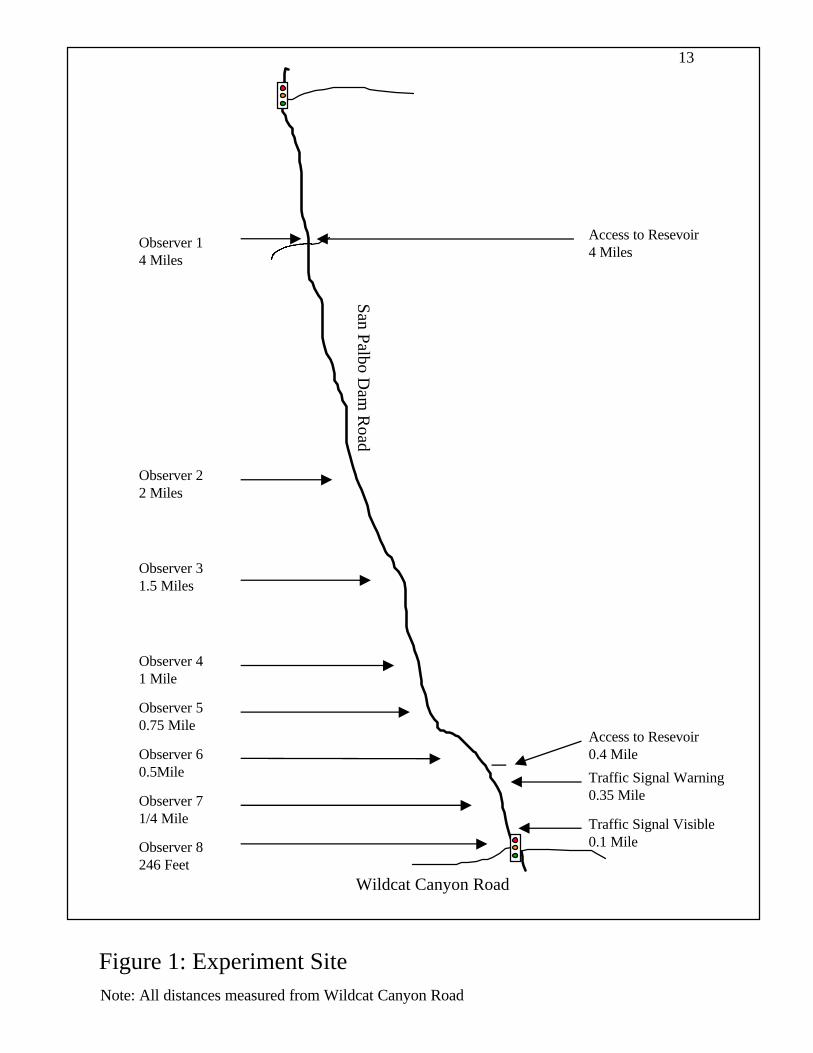
the methods used to extract the data. As regards the former, the data were collected onthe four-mile segment of southbound San Pablo Dam Road shown in Figure 1. The site,located immediately north of the intersection with Wildcat Canyon Road, is a two-lanerural highway connecting the cities of Richmond and Orinda, California. The highwayserves as a commuter alternative to a congested regional freeway. It has a posted speedlimit of 50 mph (commensurate with its design standards), some gentle horizontal andvertical curves, and a slight uphill grade (for southbound traffic) near the intersection withWildcat Canyon Road. Adequate shoulders exist throughout the segment.

The near-absence of access and egress points and the minimal overtakingmaneuvers at the site mean that vehicles maintained (approximately) their relativepositions in the traffic stream; the amount of traffic that used the two access points at theSan Pablo Dam reservoir was negligible and only a few vehicles, usually motorcycles,bypassed queues by driving on the shoulder. The downstream intersection at WildcatCanyon Road is controlled by a vehicle-actuated traffic signal, which causes a queue ofsouthbound vehicles to grow steadily during much of the morning rush.

4

To collect the data, the eight observers were stationed along the site, as shown inFigure 1. While obscured from the view of drivers, these observers used laptop computersto record the arrival times of individual vehicles at their respective observation points.The laptop computers' internal clocks were synchronized prior to the first day ofobservation and a computer program was coded to append time values to keystrokes. Theobservers recorded each vehicle's arrival time and the vehicle class by pressing a specifiedkey (i.e., "A" for automobile and "T" for commercial truck). The data format is explainedin the following section.

Figure 1 shows that at the downstream end of the site, the observers werestationed in close proximity to one another. This arrangement yielded a highermeasurement resolution for viewing disturbances shortly after they emanated from thetraffic signal where we expected them to be growing. To ensure a complete study of thequeue, the upstream-most observer was stationed four miles from the signal since it wasestimated that the effects of the queue would not be felt beyond this location. Alldistances shown in Figure 1 were carefully identified with a measuring wheel.

A pilot car, which was easily distinguished from other vehicles (in that it had abicycle mounted on its roof rack) cycled through the site during the study periods. Whentraveling southbound, its arrival times at each observation point were recorded (i.e., theobservers pressed "B" on their computer keyboards). To provide some redundancy, thedriver of the pilot car recorded the approximate times he passed each of the eightobservation points while traveling southbound. On each of the two observation days, thebeginning and ending of the study period were marked by the first and last passages of thepilot car. Furthermore, the intermediate arrival times of the pilot car were useful inprorating any (small) measurement errors made by the observers, as described in thefollowing section. A second car cycled through the site to provide the observers with anyneeded assistance; e.g., to furnish observers with "replacement" computers when batterieshad discharged.

Observations were collected from 6:45 a.m. to 9:00 a.m. on Tuesday, November18 and again on Thursday, November 20, 1997. There was no precipitation on either dayand visibility on the road was good.

4. THE DATAThe data from this study have been posted on the World Wide Web (at

http://www.ce.berkeley.edu/~daganzo/spdr.html) and are available in two forms: "raw"data, which have not been altered, and "final" data, which have been filtered in an effort tocorrect for measurement errors. This section provides a full description of these data,including our filtering processes.

The raw data are contained in a total of sixteen text files, with each file holding themeasurements made by a single observer on one of the two observation days. Forexample, file 1_A.txt holds the measurements of the upstream-most observer (i.e.,observer 1) on the first day and file 8_B.txt the measurements of the downstream-mostobserver on day 2. As an illustration, a small portion of data file 5_A.txt is shown inFigure 2. The figure shows that each vehicle arrival time is recorded in hours, minutes,

5

seconds and hundredths of seconds and is presented along with the vehicle's arrivalnumber and class.

The comment "Computer Failure" shown in Figure 2 is used to flag one particulartype of measurement error. Measurement errors came from several sources and they aredescribed below so that other researchers may use the raw data with their own filteringprocesses. From the following discussion, however, it should become apparent that, giventhe nature of the measurement errors, all reasonable filtering processes would yieldpractically indistinguishable results. It should also be clear that these errors did not erodethe integrity of the final data in any substantial way; i.e., despite the errors describedbelow, the data are arguably the most detailed and accurate of their kind.

Hardware Malfunctions. In a few instances, records were apparently not enteredby a human observer, but were due instead to some type of computer malfunction. Theseentries were easily identified because they gave rise to unduly small vehicle headways andthey were often accompanied by a rectangular symbol, rather than an "A", "B", or "T", inthe field designated for vehicle class. The raw data files include comment statements toflag each of these errant records and they have been purged from the final data.

Clock Synchronization Problems. Measurement errors also arose because thelaptop computer internal clocks were not always well synchronized. The clocks in two ofthe laptops used on the first day of observation ran ahead of their counterparts by exactlyone minute. This was made immediately evident by comparing the roadside data recordedwith these two computers with the corresponding passage times measured (approximately)by the driver of the pilot car. The asynchronization was attributed to human error insetting the internal clocks and, in the final data set, the vehicle arrival times measured withthese two computers were adjusted (i.e., reduced) by one minute. These adjustments aresummarized in Table 1a.

Regrettably, the computers' clocks were not re-synchronized immediately prior tothe second day of observation. As a consequence, by day 2, the clocks of all thecomputers had drifted by varying amounts. To salvage the second day's data, its vehiclearrival times taken at observation points 2 through 8 were adjusted as explained below.

First, the average free-flow vehicle trip times between each pair of contiguousobservation points were estimated for day 1. These estimates were made using the arrivaltimes for the first 25 vehicles observed on that day, since these vehicles did not encounterresidual queuing at the downstream intersection. The average travel times and standarderrors of the sample means are presented in Table 1b. Notably, the standard error for eachof these (seven) sample means never exceeded 1.2 seconds. The same calculations werethen repeated for day 2, with the results shown in Table 1c. The large discrepanciesbetween the measured averages on both days were attributed to synchronization error.

Thus, clock corrections that eliminated all the discrepancies between the recordedfree-flow trip times on both days were chosen. (If no correction is assigned to observer 1,then the clock correction for location j > 1 is simply the difference of the average triptimes from observer 1 to observer j on both days.) These corrections are shown in Table1d. This adjustment method was deemed to be more reliable than using the approximatetrip times measured on day 2 by the driver of the pilot car.

Computer Failure. Figure 2 shows a gap in the observations that extended foralmost four minutes and is labeled "Computer Failure." On occasion, a computer required

6

replacement (while in the field) because its battery had fully discharged. The fewreplacements that resulted in the loss of recorded observations are flagged in the raw dataas a "Computer Failure."

To address the resulting loss of information, the observation days were partitionedinto smaller mini-datasets consisting of all the vehicular information collected betweenconsecutive passages of the southbound pilot car. Ideally, each of the eight observerswould measure the same number of vehicles in each mini-dataset. This was approximatelythe case, except when a computer failure created large gaps in the recorded observations.Therefore, measurements taken (at the observation point) subsequent to a computerfailure were removed from the mini-dataset if the gap in the records exceeded one minute.In total, this truncation was performed only on two occasions, at two different observationpoints. In one of these occasions, which occurred during the penultimate mini-dataset ofday 2, the replacement computer could not be restarted in time to be useful for the lastmin-dataset. Two counts were also truncated for the last mini-dataset of day 2 becauseobservations at these locations were terminated shortly before the final passage of thesouthbound pilot car.

Human Error. All other (small) discrepancies between the vehicle counts in amini-dataset were attributed to human error, such as a missed observation or anunwarranted keystroke. The counting errors created by small glitches in computerexchanges were likewise placed in this category. Since these errors could not beindividually identified, they were prorated equally over each mini-dataset by re-normalizing the counts; i.e., each vehicle's arrival number, as recorded by a jth observer,was multiplied by the ratio N /N(j), where N(j) is the number of vehicles counted byobserver j in the mini-dataset and N is the average of the N(j) across observers. Of note,the four truncated counts discussed under “Computer Failure” were not adjusted and werenot included in the computation of an N .

On the second day, observer 5 failed to record the second passage of the pilot car.It was assumed that the observer inadvertently logged this arrival by selecting an A, as ifthe pilot car were a passenger car. A record of vehicle class was subsequently changedfrom an A to a B. This record was chosen in the maximum likelihood way so as to yieldthe same ratio of vehicle counts in the first and second mini-runs as was typical of theother observers. The standard error in this procedure should be on the order of 1 or 2vehicles.

Filtered in the above way, the final data were stored in two Excel spreadsheetsnamed D1Final.xls and D2Final.xls, for days 1 and 2, respectively. For illustrativepurposes, a portion of file D1Final.xls is shown in Figure 3. The following sectionpresents some evaluation of these data and the findings that resulted. It will becomeapparent from the figures presented in the next sections that the changes made by theabove filtering process are very minor.

7

5. SOME ANALYSISFigure 4 shows the conventional curves of vehicle count versus time, N(j,t), for

day 2, whereN(j,t) = the (filtered) cumulative number of vehicles to pass stationary observer j

by time t, measured from the first passage of the southbound pilot car, j =1,2,...,8.

Figure 4 indicates that the flow of southbound vehicles past j = 8 began to drop at around7:04 a.m. -- the reader may use a straight edge to verify the change in the trend of N(8,t)around this time. We believe that this drop in flow was caused by growth in theconflicting traffic streams at Wildcat Canyon Road, because the stop-and-go features ofN(8,t) reveal that the drop is due exclusively to an increase in the duration and frequencyof the episodes with zero flow (when "red" was displayed to southbound traffic) and notto any significant change in the slope of N(8,t) during the “green”.

Shortly following the overall flow reduction at j = 8, the slopes of some of theupstream N-curves dropped in sequence. Figure 4 includes labels indicating when theseevents took place at the various observation points. Note that the drop in slope at anobservation point j is simply the flow reduction brought about by the growing queue. Asone would expect, after the drop at j, when the queue has grown beyond this location, thevehicle trip times (i.e., the horizontal displacements) and the accumulations (i.e., thevertical displacements) between observation points j-1 and j are no longer minimum. Notethat the queue never propagated to j = 2 and thus, vehicles arrived at j = 2 without delay.This is evident because the horizontal displacements between the curves at j = 1 and j = 2did not noticeably increase from what is displayed at the beginning of the observationperiod.

Downstream curve N(8,t) continued to drop gradually until about 7:30 a.m., owingto gradual growth in the conflicting traffic streams at Wildcat Canyon Road. Quite apartfrom this effect, a final flow reduction occurred at j = 8 when, at about 8:27 a.m., a queuefrom further downstream spilled-over. This is evidenced by the reduced saturation flowsat Wildcat Canyon Road during the "green" periods, which are clearly visible in curveN(8,t).

The slope of upstream-most N(1,t) dropped at about 7:23. It is clear that thisslope change was due to a reduction in vehicle arrivals from further upstream becausecurve N(2,t) adopted the same slope (approximately) one trip time later. Similarly linkedchanges in the arrival rates at observation points 1 and 2 are visible from N(1,t) and N(2,t)at later times. Note in particular how the wiggles in N(1,t) are passed horizontally toN(2,t). This is an additional indication of the absence of queuing. (10)

The inset of Figure 4 shows that the pronounced stop-and-go patterns seen at j = 8were damped-out before reaching j = 6. Note how much smoother curve N(6,t) is thancurve N(8,t). Remarkably, however, new disturbances appeared further upstream. Insome instances, upstream traffic flow was reduced to zero as it completely jammed and afew such examples are labeled in the inset. These jams propagated upstream and alwaysdied upon (or before) reaching the upstream end of the queue. Oscillations in flow nearthe tail end of the queue appeared to be softer, as evidenced by curve N(3,t), whichexhibits a pattern of gradual slope changes. The observed fluctuations in flow neveraffected traffic upstream of the queue. There was no evidence that instabilities or jams

8

occurred in freely flowing traffic well upstream of the signal. The latter should not besurprising; if flow collapses occur at all (and we are not certain that they do), they wouldnot likely appear in a situation with a maximum flow of 1500 vehicles/hour. Theinterested reader may refer to (1) for more discussion of this issue.

Figure 5 shows the curves constructed with the final data from day 1. Study ofthese curves reveals a queue evolution similar to what was observed on day 2. Notabledifferences are that the queue on day 1 appears to reach observer 2 and to have dissipatedmore fully by the end of the observation period.

6. CONCLUSIONSThis paper has described a study of queue evolution at a highway bottleneck. The

sources of measurement error in the data collected here were explained in section 3. Thefew large errors that arose (e.g., due to failed battery exchanges) could be easily identifiedand corrected, thanks to the redundancy built into the experiment. The remaining errorswere so small that they could be distributed evenly across each mini-data-set withinsignificant changes. As an illustration of this, Figure 6 presents the unadjusted N-curvesfor both observation days. The reader is invited to compare these curves with theircounterparts in Figures 4 and 5, and to note the negligible differences. We believe theaccuracy of this experiment is comparable to experiments with loop detectors.

Visual inspection of the N-curves indicates that the queues formed in predictableways at the most obvious inhomogeneity of this facility, the traffic signal. It was alsofound that the queues dissipated in predictable ways; e.g., when vehicle arrival rates fromfurther upstream diminished and/or the bottleneck service rate increased.

There were some unusual and unexpected features in the data as well. Forexample, stop-and-go jams, uncorrelated with the traffic signal, were observed in queuedtraffic without passing. This is interesting because the absence of passing means thattraffic information is unlikely to overtake vehicles, and that theories that include suchpossibility (kinetic theory, high order fluid models, etc.) do not explain what is beingobserved here. A further puzzle is that while instabilities seem to grow in amplitude farfrom the bottleneck, the pronounced stop-and-go oscillations of the bottleneck itself wererapidly damped-out within one-half mile of it.

Perhaps these unusual observations are unique to the site studied here. Forexample, the predictability of the server (i.e., the traffic signal), and/or the low risk ofbeing overtaken, may have motivated drivers to follow downstream vehicles in unusuallyrelaxed ways. We would very much hope that other researchers would attempt toreplicate or disprove our observations at other sites. In any case, and even if strangerphenomena are observed at other sites, theories to predict these unusual features may notbe needed. The usefulness of this research for practice will come from further research.From an engineering perspective, one is most interested in predicting approximately thetime-dependent queue lengths (distances) due to control actions, and the ensuing delays.To do this acceptably well it suffices to predict the N-curves approximately at intermediatelocations (e.g., given the curves at the highway's upstream and downstream boundaries)even if one cannot predict the detailed location of all the wiggles. This seems to have beenthe objective behind Newell's simplified theory of kinematic waves (11) and it may be the

9

desirable form for future theories of highway traffic. We believe that these data andsimilar data sets obtained elsewhere can be valuable for testing practical theories thatwould predict N-curves.

ACKNOWLEDGEMENTSThe authors would like to thank Flavio Baita, Lyle DeVries, Reinaldo Garcia, JamieLawson, Raymond Lew, Michael Mauch, and Joseph Wanat for their help in collecting thedata. Research supported in part by PATH MOU-305 to the University of California,Berkeley.

10

REFERENCES

1. Daganzo, C.F., M.J. Cassidy and R.L.Bertini, Possible Explanations of PhaseTransitions in Highway Traffic, to be published in Transportation Research.

2. Herman, R. and R. Rothery (1965) Propagation of Disturbances in VehicularPlatoons in (ed. L. Edie, R. Herman, and R. Rothery), Proceedings from the ThirdInternational Symposium on Traffic Theory, 14-25.

3. Franklin, R.E. (1965) Single-Lane Traffic Flow on Circular and Straight Tracks in(ed. L. Edie, R. Herman, and R. Rothery), Proceedings from the ThirdInternational Symposium on Traffic Theory, 42-55.

4. Bleile, T. (1997) A New Microscopic Model for Car-Following Behavior in UrbanTraffic, as well as D. Manstetten, W. Krautter, and T. Schwab (1997) TrafficSimulation Supporting Urban Control Systems Development, in Proc. 4th WorldCongress in Intelligent Transport Systems, Berlin, 1997, and the analyses of thesedata in Helbing, D. and Tilch, B. “Generalized force model of traffic dynamics”(preprint.)

5. Treiterer, J. and J. Myers (1974) The Hysteresis Phenomenon in Traffic Flow in(ed. D.J. Buckley), Proceedings from the Sixth International Symposium onTransportation and Traffic Theory, 13-38.

6. Coifman, B. (1997) Time Space Diagrams for Thirteen Shock Waves, Universityof California, California PATH Working Paper, UCB-ITS-PWP-97-1.

7. Kerner, B.S., and H. Rehborn (1997) Experimental Properties of Phase Transitionsin Traffic Flow. Physics Review Letters, 79, No. 20, 4030 -4033.

8. Cassidy, M.J. and J.R. Windover (1998) Driver Memory: Motorists Selection andRetention of Individualized Headways in Highway Traffic. TransportationResearch, 32A, No 2, 129-137.

9. Makigami, Y., G.F. Newell, and R. Rothery (1971) Three DimensionalRepresentation of Traffic Flow. Transportation Science, Vol. 5, No. 3, pp. 302-313.

10. Cassidy, M. and J. Windover (1995) Methodology for Assessing Dynamics ofFreeway Traffic Flow", Trans. Res. Rec. 1484, 73-79.

11. Newell, G.F. (1993) A Simplified Theory of Kinematic Waves in Highway Traffic,Part I: General Theory. Transportation Research. 27B, 281-287.

11

LIST OF TABLES

Table 1a. Clock Synchronization Corrections, Day 11b. Free Flow Travel Times, Day 11c. Free Flow Travel Times, Day 21d. Clock Synchronization Corrections, Day 2

LIST OF FIGURES

Figure 1. Experiment SiteFigure 2. Sample from 5_A: Original Vehicle Count Files (Uncorrected)Figure 3. Sample from D1Final: Final Vehicle Count Files (Corrected)Figure 4. N-Curves, (Adjusted) Day 1Figure 5. N-Curves, (Adjusted) Day 2Figure 6. N-Curves (Unadjusted) Days 1 and 2

12

Table 1a: Clock Synchronization Corrections (min:sec)

Tuesday, November 18, 1997 (Day 1)

Observer Change

2 01:00 subtracted from all measured arrival times

3 01:00 subtracted from all arrival times measured between 6:44:33 and 8:42:14:82

(the period when a computer with an asynchronized clock was used by observer 3)

Table 1b: Free Flow Travel Times (min:sec)


Segment

Estimated Average Free

Flow Travel Time

Standard Deviation of the

Population

Standard Error of the

Sample Mean

1-2 02:16.6 00:03.7 00:00.7

2-3 00:30.3 00:01.6 00:00.3

3-4 00:40.5 00:01.7 00:00.3

4-5 00:15.2 00:02.5 00:00.5

5-6 00:24.1 00:03.2 00:00.6

6-7 00:36.2 00:06.1 00:01.2

7-8 00:25.8 00:01.0 00:00.2

Table 1c: Free Flow Travel Times (min:sec)

Thursday, November 20, 1997 (Day 2)

Segment

Estimated Average Free

Flow Travel Time

Standard Deviation of the

Population

Standard Error of the

Sample Mean

1-2 02:26.3 00:02.1 00:00.4

2-3 00:17.8 00:01.0 00:00.2

3-4 00:45.3 00:01.9 00:00.4

4-5 00:19.4 00:01.3 00:00.3

5-6 00:11.2 00:01.8 00:00.4

6-7 00:31.0 00:01.1 00:00.2

7-8 - 00:10.4 00:01.5 00:00.3

Table 1d: Clock Synchronization Corrections (min:sec)

Thursday, November 20, 1997 (Day 2)

Observer Change

2 01:09.7 subtracted from all measured arrival times

(includes 1 minute correction for original asynchronization of the clock)

3 00:02.8 added to all measured arrival times






13

Figure 1: Experiment Site

Observer 14 Miles

Observer 22 Miles

Observer 31.5 Miles

Observer 41 Mile

Observer 50.75 Mile

Observer 60.5Mile

Observer 71/4 Mile

Observer 8246 Feet

Traffic Signal Warning0.35 Mile

Traffic Signal Visible0.1 Mile

San Palbo Dam

Road

Wildcat Canyon Road

Access to Resevoir4 Miles

Access to Resevoir0.4 Mile

Note: All distances measured from Wildcat Canyon Road

14

Figure 2: Sample from F ile 5_A.txt

Location 15602 feet from observer 1


Hours Minutes Seconds Hundredths Vehicle #

Vehicle

Class

8 21 28 24 1678 A

8 21 29 99 1679 A

8 21 31 97 1680 A

8 21 35 43 1681 A

8 21 36 69 1682 A

8 21 37 74 1683 A

8 21 41 42 1684 A

8 21 43 83 1685 A

8 21 46 96 1686 A

8 21 50 37 1687 A

Computer Failure

8 25 40 12 1688 A

8 25 43 31 1689 A

8 25 46 38 1690 A

8 25 49 52 1691 A

8 25 55 72 1692 A

8 26 0 83 1693 A

8 26 2 92 1694 A

8 26 4 78 1695 A

8 26 8 46 1696 A

8 26 12 25 1697 A

15

0

500

1000

1500

2000

2500

6:44 6:58 7:13 7:27 7:41 7:56 8:10 8:25 8:39 8:53 9:08

Figure 6: Unadjusted Curves of N(j,t,)

0

500

1000

1500

2000

2500

6:44 6:58 7:13 7:27 7:41 7:56 8:10 8:25 8:39 8:53 9:08

Day 2

Day 1

some observations of highway traffic in long queues

Documents