some implications of environmental regulation on social

Social Design Engineering Series SDES-2015-23

Some implications of environmental regulation on socialwelfare under learning-by-doing of eco-products

Koji KotaniKochi University of TechnologyResearch Center for Social Design Engineering, Kochi University of Technology

Makoto KakinakaInternational University of Japan

29th September, 2015

School of Economics and ManagementResearch Center for Social Design EngineeringKochi University of Technology

KUT-SDE working papers are preliminary research documents published by the School of Economics and Management jointly with the ResearchCenter for Social Design Engineering at Kochi University of Technology. To facilitate prompt distribution, they have not been formally reviewedand edited. They are circulated in order to stimulate discussion and critical comment and may be revised. The views and interpretations expressedin these papers are those of the author(s). It is expected that most working papers will be published in some other form.

Some implications of environmental regulation on socialwelfare under learning-by-doing of eco-products∗

Koji Kotani† and Makoto Kakinaka‡

September 29, 2015

Abstract

This paper examines the significance of environmental regulation in an economywhere an eco-product supplied by a single producer is differentiated from a conventionalproduct generating negative externalities. We develop two types of the model: one is astatic model without learning effect of eco-product planning, and the other is a dynamicmodel with learning effect. We show that the regulation should be adopted when themarginal cost of the eco-product production is high enough in a static setting. In adynamic model, however, whether the regulation improves social welfare is dependentnot only on current marginal costs of the eco-product but also on the degree of dynamiclearning effect. Particularly, the regulation could improve social welfare when learningeffect is either small or large enough, while it could deteriorate social welfare in anintermediate case. Although intuitions tell us that the value of the regulation appearsto be monotonically increasing in learning effect, our results suggest that the valuepossesses a nonmonotone U-shaped feature with respect to learning effect. The optimaldecision of the regulation in a dynamic setting could be converse to that of a staticsetting, providing important policy implications of learning potentials.

Key Words: eco-product, environmental regulation, product differentiation, learning-by-doing

∗We are responsible for any remaining errors.†Professor, School of Economics and Management, Kochi University of Technology, 2-22 Eikokuji-cho,

Kochi-shi, Kochi 780-0844, Japan (e-mail: [email protected]). Correspondence pertaining to thismanuscript should be made to Koji Kotani.‡Professor, Graduate School of International Relations, International University of Japan, 777 Kokusai-

cho, Minami-Uonuma, Niigata 949-7277, Japan (e-mail: [email protected]).

1

1 Introduction

“An important objective of environmental regulation is to induce

the substitution of nonpolluting products for polluting ones

(Jorgenson and Wilcoxen (1990)).”

“Eco-products,” “green markets,” or “environmental-friendly commodities,” etc. . . Many

terminologies have been coined and commonly used in a society to represent an impure

public good that jointly plays the two roles of both private and public goods.1 This is due to

the fact that a variety of eco-products has been introduced into markets, and the importance

on the promotion of the eco-products is widely recognized to improve the environment (see,

e.g., Conrad, 2005). At the same time, various environmental regulations on conventional

polluting products generating environmental damages have been implemented by government

authorities. Since such regulations affect the output of not only the conventional product

but also the eco-product, understanding how the regulations influence the resulting outcome

would be crucial for policymakers who intend to promote the eco-product for social welfare

improvement. The objective of this study is to clarify the role of the environmental regulation

that could affect the promotion of eco-products as well as the resulting social welfare by

deriving some important policy implications related to the regulation. More specifically, the

result of this paper attempts to answer the following question: under what circumstances

should the regulation be implemented?

This paper focuses on two critical features of the eco-product: the first is that the pro-

duction technology of the eco-product is evolved through process innovation associated with

learning-by-doing; and the second is that firms producing eco-products, which generate no

negative externalities from production and consumption, compete with the producers of con-

ventional polluting goods due to their substitutability.2 Concerning the first feature, it has

been widely acknowledged that current production enhances future productivity through

1This paper uses these terminologies interchangeably. However, we mainly employ an “eco-product.”2In reality, however, eco-products may also generate a certain level of negative externalities, but in this

paper we assume that the adverse effects on the environment or humans are negligible for simplicity.

1

accumulation of experience, and such dynamic learning effect in the production process is

an essential engine of technological progress in individual firm’s as well as national levels.3

Although research and development is admitted as another important source of innovation,

there are sufficient evidences that learning-by-doing plays a crucial role for cost reduction

(see, e.g., Bellas, 1998; Argote et al., 1990; Argote and Epple, 1990; Besanko et al., 2014).

Since the nature of learning is dynamic, analysis in the framework of a dynamic setting

is worthwhile to examine how such learning effect affects the outcomes and to find some

important implications.

To capture the second feature of the eco-product in a simple manner, we consider a situa-

tion where an eco-product supplied by a single producer is differentiated from a conventional

product supplied in a perfectly competitive market. As a first approximation to reality, the

analysis assumes the single producer of an eco-product, since a newly-introduced eco-product

is usually considered an innovative product, which deserves some degree of economic rent

for the survival in a market. Moreover, in this study, learning effect can be internalized

in the technology of the single producer without any spill-over. These specifications might

be consistent with a situation where a single producer first invents and introduces an eco-

product into a market and then competes with a pre-existing conventional product due to

their substitutability.

Much work on environmental-friendly products has been done in the literature (see, e.g.,

Conrad (2005) and Bansal and Gangopadhyay (2003)). Employing a model with product

differentiation originated from consumers’ environmental awareness, they discuss firms’ in-

centives in choosing the quality or technology that sets the environmental-friendliness of

polluting products. However, there is still unsettled dispute on how much environmental

awareness incites real consumer choices for eco-products. Recent marketing researches re-

veal that although some people express high consciousness on being a green consumer in

surveys, the portion of those people is still small and such consciousness over environmen-

3For early work on learning-by-doing, see, e.g., Arrow (1962), Spence (1981), Fudenberg and Tirole (1983),Romer (1986), and Stokey (1988).

2

tally sound practices does not necessarily reflect actual consumers’ choices (see, e.g., Loureiro

et al. (2002) and Grankvist et al. (2004)). Given the evidences, this study takes a different

angle from past literature. Product differentiation between eco-products and conventional

products is assumed to derive from the distinctions of “purely” perceived quality in this

paper, while we admit that consumers’ environmental awareness may be another important

source of product distinctiveness. For example, organic products in agriculture have “cos-

metic defects” relative to the conventional ones, but healthier.4 The same type of product

differentiation can also be seen in the other industries, such as paper and pulp, where eco-

products and conventional products co-exist. Instead of a usual assumption that producers

set the environmental technology or the degree of the environmental-friendliness of their

products, this study explicitly distinguishes the eco-product from the conventional product

generating negative externalities.

In terms of environmental regulations, there has been a series of literature which exam-

ines the implications of various policies on products generating negative externalities (see,

e.g., Arora and Gangopadhyay, 1995; Cremer and Thisse, 1999; Goulder and Mathai, 2000;

Moraga-Gonzalez and Padron-Fumero, 2002; Bansal and Gangopadhyay, 2003; Eriksson,

2004; Zhu and Ruth, 2015). Whereas their focus is mainly on the incentive schemes of gov-

ernment policies such as tax and subsidy, the analysis in this paper only consider standards

or targets for environmental quality as the government policy tool for environmental regu-

lation, such as emission standards or best available control technology standard. Cropper

and Oates (1999) and Kolstad (2010) state that since in reality there are some problems of

measurement or other informational obstacles to adopt the first-best incentive policies, the

determination of actual environmental policies consists of two steps: the first is that stan-

dards or targets for the environmental quality is decided; and the second is that a regulatory

system with incentive schemes is arranged so that these standards are efficiently satisfied.

From a practical point of view, this paper pays attention to the first stage of setting the

4See Loureiro et al. (2002) for an evidence that cosmetic issues are salient in consumer choices.

3

targets or standards as a government policy tool, while the exploration of an equivalent basis

in the second step is left for future researches.5

It should also be noted that this study examines the case where the government makes

the commitment to a new environmental standard as the regulation for a sufficiently long

time, once it is set. Certainly, one may suggest that there are strategic interactions between

the government and the industry as in the cases with tax/subsidy scheme. While it could

be admitted that such strategic interactions may be present, we still restrict ourselves to

the commitment case for the two reasons. One reason is that the commitment case yields a

set of interesting results in itself and could be a benchmark analysis. It would be possible

that the basic structure of the benchmark model introduced in this paper is extended to the

one where strategic interactions exists, and such an extension should be addressed in future

researches. The other reason is based on the historical fact that once targets or standards

are devised, they tend to sustain for a sufficiently long time such as 10 years or much longer

in many countries.6 Therefore, the analysis based on the commitment seems plausible or a

good approximation to a real world.

This paper first develops a static model of the single firm producing an eco-product as

a base case, where its production technology, represented by the constant marginal cost,

is not associated with any learning effect. The environmental regulation is assumed to

raise the production cost of the conventional product and to reduce environmental damages

from the conventional product. With this approach, we show the possibility that a tighter

environmental standard on the conventional product induces social welfare improvement

through promoting the substitutable eco-product when its technology level is low enough.

This is due to the fact that when the marginal cost of the eco-product is high enough, the

5There are many studies on the role of environmental standards, like emission standards, in the discussionsof various contexts, such as abatement technology and compliance. See, e.g., Arora and Gangopadhyay (1995)and Stranlund (1997).

6For example, environmental standards for various chemicals have not changed for ten years or muchlonger in many countries (See Ministry of Environment Government of Japan (2006b) and Ministry ofEnvironment Government of Japan (2006a)) for the Japanese case, and Greenstone (2003) and many othersfor the case of United States.

4

conventional product is prevailing in the market, and environmental damages associated with

the conventional product is relatively large. In this case, the regulation on the conventional

product could reduce environmental damages significantly even though it decreases consumer

surplus.

Building upon the static model, this study next develops a dynamic model for the eco-

product production with learning effect.7 We keep the basic structure, but the main differ-

ence is that the marginal cost for an eco-product changes over time due to accumulation of

experience. In this setting, whether or not the regulation improves social welfare is highly

dependent not only on the initial marginal cost of an eco-product, but also on the degree

of dynamic learning effect. In particular, the regulation could improve social welfare when

the learning effect is either small enough or large enough, while it could deteriorate social

welfare in an intermediate case. Since the regulation enhances learning through shifting the

demand toward the eco-product, the intuition tells us that the value of the environmental

regulation appears to monotonically increase in the degree of dynamic learning effect. Our

results, however, suggest that this is not always the case. It is shown that the value of the

regulation possesses a nonmonotone U-shaped feature with respect to the degree of dynamic

learning effect, i.e., the regulation is likely to improve social welfare in a dynamic sense if the

degree of dynamic learning effect is either small enough or large enough. On the one hand,

if the degree of learning takes some intermediate values, the regulation could worsen social

welfare. This implies that the optimal decision of the regulation in a dynamic case could be

converse to that in a static case, given the same condition except the presence of learning,

providing important policy implications of learning potentials.

These results in this paper have some connection with a contentious debate of whether or

not tightening environmental standards is good for a society (Ambec et al., 2013). The claim

made by Porter (1991) and Porter and van der Linde (1995) is that tightening the standards

may trigger the firm’s innovation so that the regulation could cause everyone better off in the

7Miravete (2003) develops a similar type of the model to ours for a single producer with learning-by-doingin the context of international trade.

5

long run. On the other hand, several studies including Palmer et al. (1995) question their

viewpoint. Although the present study somewhat deals with a specific situation compared

to the general cases they describe, our result characterizes a situation where the regulation

on polluting products brings about the promotion of eco-products and enhances the process

innovation associated with learning in the production technology of eco-products. As a

result, social welfare could be increased under certain conditions. We believe that this

study provides one of the first exemplary models that support the conjecture that tightening

environmental standards makes a society better off, and this point could also be counted as

one of the main contributions.

In the next section, we elaborate on the basic elements of the model which are common

both in the static and dynamic models. The section is followed by presenting the static

model without considering learning and provides several main results. In the third section,

the dynamic model with learning effect is developed, and the steady state is analytically

characterized as a long-run outcome. We then examine the optimal decision rule of the

regulation using a numerical analysis. The results are compared with those derived in the

static model to illustrate some important implications. In the final section, we offer some

conclusions.

2 The Model

We consider an economy with a numeraire sector and an industry consisting of two sectors,

an eco-product and a conventional product. The model is written in continuous time. The

conventional product is produced in a perfectly competitive market with a constant marginal

cost, which is fixed over time. In contrast, the eco-product is a new innovative product, which

deserves some degree of monopoly rent. As a first approximation of the analysis, the eco-

product is assumed to be produced by a single producer without new entry. Technology of the

eco-product is characterized with instantaneous constant returns to scale, but its marginal

6

cost declines with output due to dynamic economies of scale through learning-by-doing, as

explained later. In this study, the only state variable is the level of marginal cost of an

eco-product. These two products are substitutes. The substitutability is assumed to come

from differences of pure perceived characteristics as a product, as mentioned in the previous

section (see, e.g., Loureiro et al. (2002) and Grankvist et al. (2004) for empirical evidences).

The other difference between the conventional product and the eco-product is that the

former entails negative externalities from consumption or production, while the latter does

not. To control pollution, the government may impose the environmental regulation on the

production of the conventional product. In order to keep the model simple and obtain clear

policy implications, it is assumed that the government decides whether or not to adopt the

regulation. The regulation precludes the negative externalities but causes the producers to

incur an additional marginal cost. Let φ ∈ {0, 1} denote the binary choice such that φ = 1

if the government adopts the regulation, and φ = 0 otherwise. Specifically, we assume that

the constant marginal cost for the conventional product is given by τ(φ) such that τ(0) = τ

and τ(1) = τ + ξ, and the pollution level per unit of the output of the conventional product

is given by ε(φ) such that ε(0) = ε and ε(1) = 0, where 0 < τ < τ + ξ < 1 and ε > 0. As

ξ becomes larger, the regulation causes a larger additional increase in the marginal cost for

the eco-product. As ε becomes larger, the production of the conventional product induces a

larger amount of pollution under no regulation. Thus, this specification captures the trade-off

relationship between an increase in the marginal cost for the conventional product under the

regulation and an increase in negative externalities through pollution under no regulation.

Notice that if the regulation is adopted, there is no pollution, i.e., ε(1) = 0.8 The

regulation in this study may be interpreted as the adoption of environmental standards

on the conventional product which reduce pollution emission to a sufficiently low level at

which negative externalities become negligible. This setting can be justified by the fact

that new standards for environmental quality are usually determined by the criterion of

8The results in what follows will not be affected significantly even if there is a positive level of pollutionunder the environmental regulation, i.e., ε(1) ∈ (0, ε).

7

“permissible concentration” or “acceptable” (see, e.g., Oates et al. (1989), Baumol and

Oates (1988) and Kolstad (2010)). Thus, in our model, both the conventional product

and the eco-product are environmental-friendly under the regulation. However, since their

substitutability does not come from environmental awareness of consumers, it is not affected

by the government decision of whether or not to adopt the regulation. This implies that the

demand for both products is totally independent of the environmental performance of the

conventional product.

Let x and y denote the consumption of an eco-product sold by the single producer and

the consumption of a conventional product in a perfectly competitive market, respectively.

Following Singh and Vives (1984), we assume that there is a representative consumer whose

preference is described by a quasi-linear utility with respect to a numeraire, q+u(x, y), where

q is the consumption of the numeraire and u(x, y) is a quadratic sub-utility with symmetric

cross-effects with u(x, y) = (x+ y)− (x2 + y2 + 2γxy)/2. The parameter γ ∈ [0, 1) measures

the degree of product differentiation between the eco-product and the conventional product.

The sufficient condition ∆ = 1−γ2 > 0 ensures that the sub-utility function u(x, y) is strictly

concave. If γ = 0 the conventional product and the eco-product are viewed as independent,

but as γ → 1 these products become closer to perfect substitutes.

At each instantaneous time, the representative consumer maximizes the utility subject

to his budget constraint I = q + px+ τ(φ)y, where p is the price of the eco-product decided

by the single producer. Notice that the price of the conventional product is equal to its

marginal cost τ(φ) due to the perfect competition. The first-order conditions yield the

following demand functions:

x∗(p, φ) =1− γ(1− τ(φ))

1− γ2− 1

1− γ2p; y∗(p, φ) =

(1− τ(φ))− γ1− γ2

+γ

1− γ2p. (1)

The demand for the eco-product is decreasing in p while the demand for the conven-

tional product is increasing in p, i.e., x∗p < 0 and y∗p ≥ 0 with equality if γ = 0. Since

8

τ(0) = τ < τ + ξ = τ(1), the environmental regulation increases the demand for the eco-

product but decreases the demand for the conventional product, i.e., x∗(p, 0) < x∗(p, 1)

and y∗(p, 0) > y∗(p, 1). Using demands (1), we obtain instantaneous consumer surplus,

S(p, φ) ≡ u(x∗(p, φ), y∗(p, φ))− px∗(p, φ)− τ(φ)y∗(p, φ), and the instantaneous profit for the

single producer, π(p, φ, c) ≡ (p−c)x∗(p, φ), where c is the marginal cost for the eco-product.9

For simplicity, we assume that the instantaneous negative externalities from the conven-

tional product depends only on the total pollution, which is represented by the pollution

level per unit of the output of the conventional product times the conventional product con-

sumption, ε(φ)y∗(p, φ). Specifically, the instantaneous negative externalities are given by

E(p, φ) = Γ(ε(φ)y∗(p, φ)), where Γ is strictly increasing and strictly convex with Γ(0) = 0.

Notice that to focus on the dynamics of technological progress, we do not consider the evolu-

tion of the concentration of pollution.10 Then, instantaneous social welfare is simply defined

as T (p, φ, c) ≡ π(p, φ, c) + S(p, φ)− E(p, φ).11

The central assumption is that technology of an eco-product exhibits instantaneous con-

stant returns to scale, but its marginal cost, c, is reduced over time as the single producer

accumulates output, i.e., the level of marginal cost is reduced due to the accumulation of

experience. Unlike the standard learning curve specification as in Spence (1981), we also

consider the depreciation of experience, or in an alternative interpretation, the existence

of potential adjustments costs in the accumulation of such experience, so that some min-

imum production level is required at every period to ensure a net reduction of the single

producer’s marginal cost. Several authors claim that such depreciation of knowledge is also

important in reality and empirically show some evidence (see, e.g., Argote et al. (1990) and

Benkard (2000)).12 The existence of such a knowledge depreciation allows us to identify a

9For just a explanatory reason, consumer surplus in our definition does not include the negative external-ities that come from pollution associated with the consumption and production of the conventional product.Such negative externalities are captured separately in this paper.

10For the model setting with the evolution of technology and the concentration of pollution, see, e.g.,Goulder and Mathai (2000).

11Instantaneous social welfare could be described by a more general form of T (π(p, φ, c), S(p, φ), E(p, φ)).However, the main results in this study are not changed in general.

12For a similar setup of the model using the learning curve with knowledge depreciation, see, e.g., Miravete

9

steady state, which could be important to analyze a long-run outcome in an economy. For

analytical tractability, the reduction in the marginal cost is assumed to be described as the

following state equation:

c = −λ[x∗(p, φ)− σ(c)], (2)

where λ ≥ 0 represents the marginal cost reduction effect per unit of output, or simply the

degree of dynamic learning effect, and σ(c) captures a situation where the value of experience

depreciates over time.

For the consistency with empirical regularity, it is assumed that σ(c) = η− δc with η > 0

and δ > 0 and that the marginal cost of the eco-product in the initial period is not large

enough so that c0 < η/δ.13 With this specification of the state equation (2), the speed of

technological improvement is increased with higher output, lower knowledge depreciation

and higher learning effect, as long as x∗(p, φ) > σ(c). In addition, it may be consistent with

a real observation in terms of knowledge accumulation. If the learning parameter λ is large,

likewise the speed of knowledge accumulation as well as that of knowledge depreciation.

Therefore, it agrees with a situation where “knowledge or skills that can be quickly obtained

tends to be forgetful very shortly if they are not in practice.” Conversely, for small λ, the

speed of knowledge accumulation is slow, likewise knowledge depreciation. Contrary to the

high learning, the skills that are once obtained would be forgetful very slowly. Finally, notice

that when there is no dynamic learning effect, i.e., λ = 0, our problem is reduced to a static

single producer’s problem with two differentiated products, in which one is produced by a

single producer and the other is produced in a perfectly competitive market.

To analyze the pricing of the eco-product and the environmental regulation, we consider

an economy which extends over the following two steps. In step 1, the government decides

whether or not to adopt the regulation on the production of the conventional product.14

(2003).13This assumption excludes a case in which the knowledge depreciation rate is negative, i.e., σ(c) < 0.14As mentioned in the previous section, the government is assumed to make the commitment to a newly-

10

The decision affects the constant marginal cost for the conventional product, τ(φ), and the

pollution level per unit of the output of the conventional product, ε(φ). In step 2, taking the

government’s decision, φ, as given, the single producer producing the eco-product decides

the pricing schedule over time so that the present value of the profits is maximized. Then,

consumption and production of the eco-product and the conventional product take place in

each time.

3 Static Model

This section examines a static case where the single producer chooses the optimal price of the

eco-product taking the government policy φ and the marginal cost c as given. A static case

is equivalent to the one in which there is no dynamic learning effect, i.e., λ = 0. In this case,

since the marginal cost for the eco-product is constant over time, the single producer simply

maximizes its instantaneous profit π(p, φ, c) with respect to p, taking φ and c as given. The

first-order condition yields the optimal price of the eco-product:

pM(φ, c) =c+ τ(φ)γ + 1− γ

2. (3)

Using equation (3), we obtain the consumptions of the eco-product and the conventional

product and consumer surplus, the single producer’s profit and the negative externalities:

xM(φ, c) ≡ x∗(pM(φ, c), φ), yM(φ, c) ≡ y∗(pM(φ, c), φ), SM(φ, c) ≡ S(pM(φ, c), φ), πM(φ, c) ≡

π(pM(φ, c), φ, c), and EM(φ, c) ≡ E(pM(φ, c), φ). In order to make our analysis simple, in the

rest of this paper, we assume that the solution is interior in the sense that the consumption

levels of the eco-product and the conventional product are positive.

Based on the above discussions, we derive the impact of technological improvement of

the production of the eco-product, which exhibits a decline in its marginal cost. As in the

introduced environmental standard for a sufficiently long time. Although we admit that there may be theprecommitment issues with strategic interactions between the government and the single producer of theeco-product, we believe that the commitment could be a first approximation to a real world.

11

standard static monopoly theory, it is directly shown that, for any φ ∈ {0, 1}, technologi-

cal progress in the production of the eco-product decreases the optimal eco-product price;

increases the output of the eco-product; decreases the output of the conventional product

and the negative externalities; and increases consumer surplus as well as the profit for the

single producer (see Claim 1 in the Appendix for the proof).15 Technological progress in the

eco-product not only substitutes the conventional product into the eco-product through a

decline in the price of the eco-product but also improves social welfare through the increase

in consumer surplus and the profit for the single producer and the decrease in the negative

externalities.

3.1 Environmental Regulation

In this subsection, we consider the impact of the environmental regulation without dynamic

learning effect (λ = 0). The regulation affects the optimal price of the eco-product through

raising the market price of the conventional product. Then, we deduce the following results

(see the Appendix for the proof):

Proposition 1 (Environmental Regulation) Suppose λ = 0. Then, the environmental

regulation (1) increases the optimal price of the eco-product; (2) increases the output of the

eco-product but decreases the output of the conventional product; and (3) decreases consumer

surplus but increases the profit for the single producer.

The regulation allows the single producer of the eco-product to take advantage through in-

creasing the production cost of the conventional product. Similar to the case of technological

improvement, the regulation promotes the eco-product, reduces the conventional product,

and vanishes its negative externalities. However, the effects on the price of the eco-product

and consumer surplus have the opposite direction. In this case, promoting the eco-product

with preferable environmental performance can be achieved at the expense of consumer sur-

plus. In contrast to the case where technological progress always improves social welfare,

15For φ = 1, there are no negative externalities for any technology level.

12

whether the regulation improves social welfare depends on the degree of positive impacts

on the negative externality and the single producer’s profit and the degree of the negative

impact on consumer surplus.

3.2 Government’s Decision Problem

We now find the optimal government’s decision regarding the regulation in step 1 when

there is no dynamic learning effect. The government chooses to adopt the regulation (φ = 1)

if social welfare is larger under the regulation than under non-regulation, i.e., ∆TM(c) ≡

T (pM(1, c), 1, c)− T (pM(0, c), 0, c) > 0, where ∆TM(c) represents the value of the regulation

or the effect of the regulation on social welfare. Then, we obtain the following result related

to the optimal policy as a possible case (see the Appendix for the proof):

Proposition 2 (Environmental Policy) Suppose λ = 0. Then, there may exist a unique

value cM > 0 such that the optimal policy is to impose the environmental regulation on the

conventional product if c > cM ; and not to impose the regulation if c < cM .

The conditions for the uniqueness of cM > 0 are ∆TM(0) < 0 and ∆TM(1) > 0. These

require that if the marginal cost of the eco-product is small enough so that the eco-product

is diffused enough in the market, the regulation cannot be justified from the standpoint of

social efficiency, and that if the marginal cost of the eco-product is large enough so that the

conventional product is diffused enough in the market, the regulation can be justified.

The logic behind Proposition 2 is as follows. The value of the regulation or the effect of

the regulation on social welfare can be divided into the three elements and is rewritten by

∆TM(c) = ∆SM(c)+∆πM(c)+Γ(εyM(0, c)), where ∆SM(c) ≡ SM(1, c)−SM(0, c) represents

the value of the regulation related to consumer surplus, ∆πM(c) ≡ πM(1, c) − πM(0, c) the

value of the regulation related to the profit for the single producer, and Γ(εyM(0, c)) the

value of the regulation related to environmental damages. As shown in Proposition 1, the

introduction of the regulation reduces consumer surplus (∆SM(c) < 0), increases the profit

13

for the single producer (∆πM(c) > 0), and vanishes environmental damages (Γ(εyM(0, c)) >

0).

When the cost of the eco-product is low, the sales of the eco-product is already high and

those of the conventional product is already low due to their substitutability. In this case,

the reduction in environmental damages from the conventional product, associated with the

regulation, may not make up for the increased loss in consumer surplus, even though the

regulation still induces a demand shift from the conventional product toward the eco-product,

i.e., ∆SM(c)+∆πM(c)+Γ(εyM(0, c)) < 0 for a low c. That is, since the negative externalities

under non-regulation is relatively small due to relatively small demand for the conventional

product, the merit of the regulation from vanishing the negative externalities cannot offset

the negative effect on consumer surplus. Thus, the regulation cannot be justified.

In contrast, when the cost of the eco-product is high, the sales of the eco-product is low

and those of the conventional product is high. In this case, the reduction in environmental

damages associated with the regulation may make up for the increased loss in consumer

surplus, i.e., ∆SM(c)+∆πM(c)+Γ(εyM(0, c)) > 0 for a high c. Since the negative externalities

under non-regulation are relatively large due to relatively large demand for the conventional

product, the merit of the regulation from vanishing the negative externalities dominates the

negative effect on consumer surplus. Thus, adopting the regulation can be justified even

though consumer surplus is reduced as a result.

Examination of the impact of a change in ξ and ε is important for policy makers to decide

whether or not the regulation should be adopted. At the critical value, it must hold that

∆TM(cM) = 0. Our specification of the model implies that the critical value cM is decreasing

in the pollution level per unit of the output of the conventional product, ε (see Claim 2 in

the Appendix). A rise in the pollution level ε increases environmental damages under non-

regulation, which implies that the value of the regulation related to environmental damages

becomes large or the regulation becomes more attractive. Thus, the region of c, in which

adopting the regulation is optimal (c > cM), becomes larger as ε increases. Furthermore, our

14

specification also states that the critical value cM is increasing in the effect of the regulation

on the marginal cost of the conventional product, ξ (see Claim 2 in the Appendix). A rise in

ξ raises the price of the conventional product, which reduces consumer surplus. Thus, when

ξ is higher, the regulation becomes less attractive and the region of c, in which adopting the

regulation is optimal (c > cM), becomes smaller.

4 Dynamic Model under Learning-by-Doing

The previous section has examined the static model under the assumption that there is no

dynamic learning effect. We now assume a positive dynamic learning effect, i.e., λ > 0.

One important distinction between the static and the dynamic settings is that the marginal

cost of the eco-product is exogenously given in the static setting, while it is evolved through

learning process in the dynamic setting. This section first characterizes the steady state as a

long-run outcome under the optimal price schedule over time decided by the single producer

of the eco-product at step 2. We then explain the government’s decision problem at step 1

in which the government can decide whether or not to adopt the regulation φ ∈ {0, 1} at

time t = 0 without possibility of changing the policy after the decision.

The single producer’s problem is to maximize the present value of her profits, while con-

sidering the environmental regulation and the learning effect induced by current production

through her pricing decisions. This problem can be stated as maxp∫∞

0π(p, φ, c)e−rtdt sub-

ject to c = −λ[x∗(p, φ)− σ(c)] and c(0) = c0, where r > 0 represents the discount rate. The

value of x∗(p, φ) is the demand for the eco-product derived in equation (1). Applying the

dynamic optimal control with the Hamiltonian, HF = π(p, φ, c) − µfλ[x∗(p, φ) − σ(c)], the

equilibrium of our model solves the following set of generalized Hamilton-Jacobi conditions:

x∗(p, φ) + (p − c − λµf )x∗p(p, φ) = 0 and µf = (r + λδ)µf + x∗(p, φ). This problem yields a

15

linear differential system:

p

c

= M

p

c

+

λη−(r+λδ)[1−γ(1−τ(φ))]2

(1−γ2)λη−λ[1−γ(1−τ(φ))]1−γ2

where M =

r + λδ − r+2λδ2

λ1−γ2 −λδ

. (4)

The matrix M is independent of the government’s decision.

For any φ ∈ {0, 1}, a pair of the marginal cost and the price of the eco-product,

(c(φ), p(φ)), at which c = p = 0 in the linear differential system (4), is called a steady state.

A steady state is stable if c and p converge to c and p, respectively (see, e.g., Kamien and

Schwartz (2012)). The specification of our dynamic model implies that for any φ ∈ {0, 1},

there exists a unique steady state (c(φ), p(φ)), and that the unique steady state is sta-

ble if the degree of product differentiation between the eco-product and the conventional

product is small enough so that det(M) < 0 or γ < γ, where γ ≡ (1 − r+2λδ2δ(r+λδ)

)1/2 (see

Claim 3 in the Appendix).16 In the rest of the paper, we assume γ ∈ [0, γ). Under this

assumption, for any φ ∈ {0, 1}, the equilibrium path of state variable c is described by

ct(c0, φ) = [c0 − c(φ)]ekt + c(φ), where k = r2− r+2λδ

2[1− 2λ

(1−γ2)(r+2λδ)]12 ∈ (−λδ, 0).

Given a state variable c = ct(c0, φ), the optimal price of the eco-product decided by the

single producer is represented by:

p(φ, c) = α1c+ α2(φ), (5)

where α1 = (1−γ2)(k+λδ)λ

> 0 and α2(φ) = −k(1−γ2)λ

c(φ)− η(1− γ2) + 1− γ(1− τ(φ)).17 Then,

given φ and c, the equilibrium levels of the outputs of the eco-product and the conventional

product, consumer surplus, the profit for the single producer, and the negative externalities

can be respectively represented by x(φ, c) ≡ x∗(p(φ, c), φ), y(φ, c) ≡ y∗(p(φ, c), φ), S(φ, c) ≡

S(p(φ, c), φ), π(φ, c) ≡ π(p(φ, c), φ, c), and E(φ, c) ≡ E(p(φ, c), φ).18 It is assumed that

16If γ < γ, the steady state is a saddlepoint and is stable. In contrast, if γ > γ, the state variable neverconverges to the steady state.

17Since k is independent of φ, α1 is also independent of φ, but α2(φ) is dependent of φ.18Our specification implies that for given φ ∈ {0, 1} with c0 > c(φ), the marginal cost of the eco-product

16

any variable is interior in the equilibrium path in the sense that the production and the

consumption of the eco-product and the conventional product are always positive. Figure 1

indicates the general direction of movement that (c, p) would take from any location. c is

momentarily stationary along a path as the c = 0 locus is crossed and k is stationary as the

k = 0 locus is crossed.

4.1 Steady State as Long-Run Outcome

This subsection characterizes the steady state as a long-run outcome. For any φ, by applying

the Cramer’s Rule to the system (4) with p = c = 0, we obtain the price and the marginal

cost of the eco-product in the steady state, (c(φ), p(φ)), which derive the corresponding

outputs of the eco-product and the conventional product, consumer surplus, the profit for

the single producer, and negative externalities in the steady state: x(φ) ≡ x∗(p(φ), φ),

y(φ) ≡ y∗(p(φ), φ), S(φ) ≡ S(p(φ), φ), π(φ) ≡ π(p(φ), φ, c(φ)), and E(φ) ≡ E(p(φ), φ).

Notice that all instantaneous variables above are a function of the government’s binary

choice variable φ. By the state equation (2), it must hold that x(φ) = σ(c(φ)) in the steady

state, which yields:

σ(c(φ)) =(r + λδ)[1− c(φ)− γ(1− τ(φ))]

2(r + λδ)(1− γ2)− λ. (6)

The condition x(φ) = σ(c(φ)) states that the output of the eco-product is inversely related

to the level of knowledge depreciation in the steady state. If a large degree of knowledge

depreciation is associated with the eco-product production, the single supplier would keep a

higher level of the production to maintain the knowledge related to the production process.

Notice that in this study, the dynamic learning effect is only the source of technological

is monotone decreasing over time. Thus, the output of the eco-product and consumer surplus are monotoneincreasing over time, while the price of the eco-product, the output of the conventional product and thenegative externatilities are monotone decreasing over time. In an infinite horizon autonomous problem withjust one state variable, if there is an optimal path to a steady state, the state variable is monotonic overtime, and the steady state must be a saddlepoint. This is illustrated in Figure 1.

17

progress, and the degree of dynamic learning effect, λ, influences the steady state through

the state equation c = −λ[x∗(p, φ) − σ(c)]. Concerning the effect of a change in λ on the

steady state, our specification implies that for any φ, if λ > 0 and γ < γ, in the steady

state, an increase in λ reduces the marginal cost and the price of the eco-product; raises the

output of the eco-product; reduces the output of the conventional product and the negative

externalities; and increases consumer surplus (see Claim 4 in the Appendix). These results

imply that the larger learning effect induces a decline in the price of the eco-product through

technological progress. This encourages people to shift the demand from the conventional

product to the eco-product, which reduces environmental damages and improves consumer

surplus in the long-run.

4.2 Environmental Regulation

We now examine the effect of the environmental regulation on the steady state as a long-run

outcome. Solving equation (6) yields the marginal cost of the eco-product in the steady

state, c(φ). The impact of the regulation on the marginal cost of the eco-product in the

steady state is described by:

c(0)− c(1) =γ

2δ(γ2 − γ2)(τ(1)− τ(0)) > 0. (7)

Then, we deduce the following results related to production technology of the eco-product

(see the Appendix for the proof).

Proposition 3 (Environmental Regulation and Marginal Cost in Steady State)

Suppose λ > 0 and γ < γ. Then, the environmental regulation reduces the marginal cost

of the eco-product in the steady state, i.e., c(0) > c(1). Furthermore, the impact of the

regulation on the marginal cost, c(0)− c(1), is increasing in the degree of dynamic learning

effect, λ.

18

This proposition consists of two important implications. First, the regulation would trigger

the firm’s innovation (in this case, not product innovation but process innovation) on the eco-

product production technology. Second, the impact of the regulation is more significant when

the technology entails a larger learning effect. These are due to the fact that the regulation

encourages the demand to shift toward the eco-product, which enhances the learning effect

more effectively. This discussion may be similar to the one in the infant industry protection

arguments, where the government supports targeted infant industries for future returns at

the expense of the current distortion.

Based on Proposition 3 with equation (7), we examine the impact of the regulation on

the price of the eco-product in the long-run, which is written by:

p(1)− p(0) = [pM(1, c0)− pM(0, c0)]− 1

2

[1 +

λδ

r + λδ

](c(0)− c(1)). (8)

This impact can be divided into two sub-effects. The first sub-effect, pM(1, c0)− pM(0, c0) =

γ2(τ(1)− τ(0)) > 0, may be regarded as the ‘substitution’ effect in the sense that this term is

associated with a rise in the marginal cost of the conventional product under the regulation.

This induces a rise in the price-cost margin of the eco-product through the demand shift

from the conventional product toward the eco-product. This sub-effect is consistent with

the effect of the regulation in the static setting in Proposition 1. The second sub-effect,

12[1+ λδ

r+λδ](c(0)− c(1)) > 0, may be considered as the ‘cost-reduction’ effect of the regulation

in the sense that this term is associated with a decline in the marginal cost of the eco-product,

which is caused by enhancing learning effect through the regulation, as in Proposition 3.

The impact of the regulation on the price of the eco-product is ambiguous since an increase

in the demand for the eco-product associated with a rise in the price of the conventional

product ambiguously affects the optimal price of the eco-product for the single producer. In

fact, which sub-effect dominates the other determines the direction of the impact. Proposi-

tion 3 showed that a large degree of learning effect, λ, makes the regulation more effective in

19

the sense that c(0)− c(1) is increasing in λ. Thus, if learning effect is large enough so that

the cost-reduction effect dominates the substitution effect, the regulation reduces the price of

the eco-product. This result is in contrast to the result that the regulation always raises the

price of the eco-product in the static setting. The crucial difference between the static and

the dynamic settings is that the cost-reduction effect associated with learning effect exists

in the dynamic setting while it does not exist in the static setting.

Concerning how the regulation affects the promotion of the eco-product, we consider the

impact of the regulation on the outputs of the eco-product and the conventional product in

the steady state. Use equations (1) and (8), we obtain:

x(1)− x(0) = [xM(1, c0)− xM(0, c0)] +1

2(1− γ2)

[1 +

λδ

r + λδ

](c(0)− c(1)) > 0; (9)

y(1)− y(0) = [yM(1, c0)− yM(0, c0)]− γ

2(1− γ2)

[1 +

λδ

r + λδ

](c(0)− c(1)) < 0, (10)

where xM(1, c0)− xM(0, c0) = γ(τ(1)−τ(0))2(1−γ2)

> 0 and yM(1, c0)− yM(0, c0) = − (2−γ2)(τ(1)−τ(0))2(1−γ2)

<

0. The regulation promotes the eco-product but reduces the output of the conventional

product, which in turn reduces the marginal cost of the eco-product through learning effect.

This continued mechanism further strengthens the promotion of the eco-product, i.e., x(1) >

x(0) and y(1) < y(0). Similar to the previous analysis, the impact can be divided into the

substitution and the cost-reduction effects. The cost-reduction effect associated with learning

effect amplifies the impact compared to the static case in Proposition 1. Furthermore, a rise

in λ intensifies the impact of the regulation on the marginal cost of the eco-product (as shown

in Proposition 3), which in turn increases the impacts of the regulation on the outputs of

the eco-product and the conventional product in equations (9) and (10).

We now discuss the relation between the regulation and the long-run effect on social

welfare. As in the static case, the impact of the regulation on social welfare in the steady

state can be described by the value of the regulation in the steady state, which is written

by ∆T = ∆S + ∆π + Γ(εy(0)), where ∆S ≡ S(1)− S(0) and ∆π ≡ π(1)− π(0) represents

20

the impact of the regulation on consumer surplus and the profit for the single producer

in the steady state, respectively. If the value of the regulation is positive, adopting the

regulation improves social welfare in the steady state. In contrast, if the value is negative,

the regulation reduces social welfare in the steady state. The expression of the value implies

that the value can be divided into the three sub-values: the values related to the profit for

the single producer, consumer surplus, and negative externalities.

First, the value of the regulation related to the profit is described by ∆π = x(1)m(1)−

x(0)m(0), where m(φ) ≡ p(φ) − c(φ) is the price-cost margin under the government policy

φ. By equations (7) and (8), the impact of the regulation on the price-cost margin is:

m(1)− m(0) = [pM(1, c0)− pM(0, c0)] +γ

2

[1 +

1− δ(1− γ2)

δ(γ2 − γ2)

](τ(1)− τ(0)). (11)

Assuming that 1 − 1/δ < γ2 < γ2, the impact of the regulation on the price-cost margin is

positive and increasing in λ. Noticing that the impact of the regulation on the output of

the eco-product, x(1)− x(0), is positive and increasing in λ by the previous discussion, the

value of the regulation related to the profit, ∆π, is also positive and increasing in λ. The

regulation enhances the monopolistic power by raising the cost of the conventional product,

and this tendency is strengthened as the learning effect is more significant.

Second, concerning the value of the regulation related to consumer surplus in the steady

state, whether or not the regulation increases consumer surplus is in general ambiguous,

i.e., the sign of ∆S is ambiguous. This is due to the fact that the increased price of the

conventional product has a negative impact on consumer surplus, while the reduced price of

the eco-product due to the learning effect has a positive impact. Furthermore, differentiating

∆S with respect to λ yields:

∂(∆S)

∂λ=

rδ(γ2 − γ2)

2(r + λδ)2(1− γ)2[x(1)2 − x(0)2] > 0,

21

which implies that ∆S is increasing in λ. A larger degree of dynamic learning effect intensifies

the reduction of the price of the eco-product, which makes the regulation more attractive

from the standpoint of consumer surplus. This suggests the possibility that the regulation

could reduce consumer surplus in the steady state when λ is small, while it could increase

consumer surplus when λ is large.

Third, the value of the regulation related to environmental damages in the steady state,

Γ(εy(0)), is always positive, but is decreasing in λ. A large λ intensifies the demand shift

from the conventional product toward the eco-product under non-regulation. This in turn

reduces environmental damages associated with pollution from the conventional product

y(0). That is, if the learning effect is more significant, the regulation becomes less attractive

from the perspective of environmental issues in the steady state.

The above discussions of the three sub-values show that the entire value of the regulation

in the steady state, ∆T , is closely dependent on λ. In general, the relationship between

the value of the regulation and the degree of dynamic learning effect is complex. In Figure

2, the graph of the value of the regulation related to environmental damages, Γ(εy(0)), is

described by the thick curve that is decreasing in λ, and the graph of the value related to

total surplus (defined as consumer surplus plus the profit for the single producer), ∆S+∆π,

by the dotted curve that is increasing in λ. For the better understanding of some insights

of the dynamics different from those of the static setting, Figure 2 illustrates an interesting,

plausible case where the graph of the value of regulation in the steady state (vertical sum of

the thick and dotted curves) is described by the convex and U-shaped curve. The sufficient

condition for this is that environmental damages are relatively sensitive to the output of the

conventional product such that the convexity of Γ is large enough. Moreover, in Figure 2, it

is assumed that a larger learning effect causes the regulation to improve consumer surplus

in the steady state such that ∆T > 0 with λ large enough, and that a small learning effect

causes environmental damages under non-regulation to be significantly large due to small

demand shift from the conventional product such that ∆T > 0 with λ small enough.

22

A distinguished feature in this plausible case is that the graph of the value of the reg-

ulation, ∆T , determines the region of λ in which the regulation improves or reduces social

welfare in the steady state. In this case, a region of λ > 0 can be divided into the fol-

lowing three sub-regions: ∆T > 0 in the sub-region λ < λ1 and in the sub-region λ > λ2;

and ∆T < 0 in the intermediate sub-region λ ∈ (λ1, λ2). Focusing on this situation, we

summarize the above results:

Proposition 4 (Environmental Regulation and Steady State) Suppose λ > 0 and

1 − 1/δ < γ < γ. Then, there may exist a unique pair of values, λ1 and λ2 with 0 <

λ1 < λ2, such that the environmental regulation reduces social welfare in the steady state if

λ ∈ (λ1, λ2), while it improves social welfare in the steady state if λ < λ1 or λ > λ2.

To understand the intuition behind this, suppose first that λ is small enough so that λ < λ1.

In this case, learning effect is so small that the demand shift toward the eco-product is not

so large, and thus environmental damages in the steady state is still relatively large under

non-regulation, i.e., the value of the regulation related to environmental damages is high.

Even though the regulation reduces total surplus (consumer surplus plus the profit for the

single producer) in the steady state, or the value of the regulation related to total surplus is

negative, the regulation could improve social welfare in the steady state.

Suppose next that λ is large enough so that λ > λ2. In this case, learning effect causes

the regulation to increase total surplus through a decline in the price associated with a

significant cost reduction of the eco-product, i.e., the value of the regulation related to total

surplus is positive. In addition, the value of the regulation related to environmental damages

is still positive even though large learning effect makes environmental damages in the steady

state to be relatively small under non-regulation. As a result, the regulation improves social

welfare in the steady state.

It should be important to understand the difference in the reason why the regulation im-

proves social welfare in the steady state between the above two polar cases. When λ is large,

the regulation improves social welfare due to its role in increasing total surplus (consumer

23

surplus plus the profit for the single producer) through promoting technological progress,

not in vanishing environmental damages. In contrast, when λ is small, the regulation im-

proves social welfare due to its role in vanishing environmental damages, not in promoting

technological progress.

More importantly, Proposition 4 shows an intermediate case of λ ∈ (λ1, λ2), where the

value of the regulation in the steady state is negative. In contrast to the two polar cases

mentioned above, there may be a range of λ in which the regulation clearly has a negative

impact on social welfare in the long-run. In this case, the value of the regulation related to

total surplus is negative due to the reduction in consumer surplus caused by the regulation.

This negative effect of the regulation cannot be offset by the positive value of the regulation

related to environmental damages.

Note that Proposition 4 examined the impact of the regulation only on the long-run

outcome in the steady state, but did not say anything about the government’s optimal

policy in a dynamic setting. The optimal decision rule of the regulation depends on whether

the current value of social welfare, which must be evaluated over all the path, is increased

or decreased by the regulation. In other words, it depends on whether the current value of

the regulation over time is positive or negative. In a later section, it will be shown that the

non-monotone U-shaped property in the value of the regulation at the steady state implies

the non-monotone U-shape in the current value of the regulation.

Given this U-shaped property in the current value of the regulation under dynamic set-

tings, we can deduce some important policy implications by making comparisons of the

static and dynamic cases with the government decision. For example, suppose that an initial

marginal cost c0 is larger than cM , i.e., c0 > cM . In the absence of learning, the situation

simply becomes static and the optimal decision of the government is to adopt the regulation,

as shown in Proposition 2. However, the above U-shaped feature in the dynamic setting

implies that the optimal decision could be reversed, especially when the degree of dynamic

learning effect is in some intermediate range. Therefore, the optimal decision of the regula-

24

tion in the dynamic case can be in stark contrast to that of the static case. Unfortunately,

the current value of the regulation is too complex to be analytically characterized. Numeri-

cal analysis will be employed to illustrate the U-shaped property of the current value of the

regulation and to elaborate on various intuitions in a dynamic setting for the plausible range

of parameters. For this purpose, we next introduce the concept of the current value of the

regulation and explain the optimal decision of the government in a dynamic setting before

we go to numerical analysis.

4.3 Government’s Decision Problem

Until the previous subsection, we have examined an economy with dynamic learning effect

in step 2, taking the government policy φ as given, and have analyzed the impact of the

regulation mainly on the steady state outcomes. This subsection discusses the government’s

decision problem of whether or not to adopt the regulation at the initial period and formally

introduce the current value of the regulation in step 1, which is the basis for numerical

analysis in a later section.

The government’s problem is to maximize the present value of social welfare over time,

consisting of consumer surplus, the profit for the single producer and the negative external-

ities, taking into account the pricing decision rule made by the single producer of the eco-

product. Since instantaneous social welfare is described by T (φ, c) = S(φ, c)+π(φ, c)−E(φ, c)

for any state variable c, the government’s decision problem in time t = 0 can be restated as

maxφ∈{0,1}W (φ, c0) ≡∫∞

0T (φ, ct(c0, φ))e−rtdt, where ct(c0, φ) is the equilibrium path, and

W (φ, c0) is the present value of social welfare, taking φ and c0 as given.

By simple calculations, W (φ, c0) can be rewritten byW (φ, c0) = α0(φ)+α1(φ)c0+α2(φ)c20,

where αl(φ) is constant for l ∈ {0, 1, 2} and φ ∈ {0, 1}. Then, given c0, the government’s

optimal decision is to adopt the regulation if W (1, c0) > W (0, c0) or

∆W = W (1, c0)−W (0, c0) =

∫ ∞0

[T (1, ct(c0, 1))− T (0, ct(c0, 0))]e−rtdt > 0, (12)

25

and not to adopt the regulation if ∆W < 0, where T (1, ct(c0, 1))− T (0, ct(c0, 0)) is the differ-

ence in instantaneous social welfare between under the regulation and under non-regulation.

The value of ∆W can be considered the current value of the regulation.

It should be noted that the present paper considers only a situation where there are two

feasible choices by the government: to adopt the regulation and not to adopt it. In reality,

however, there are more than two feasible choices. When the government has a finite or an

infinite number of feasible policies, {φn}, instead of two feasible choices, it can find the opti-

mal policy φn∗ such that W (φn∗ , c0) = maxnW (φn, c0). However, for our primary purpose in

discussing the relations between dynamic learning effect and the regulation, we believe that

analyzing our simple setting with two feasible choices suffices as a simple approximation of

the assessment of the government policy.

5 Numerical Analysis

In this section, we explore some numerical examples of both the static model and the dynamic

model to illustrate the results and their intuitions. The focus is on how dynamic learning

effect can affect the optimal decision of the government compared to that in a static case.

We also show that the current value of the regulation (12) could possess a non-monotone U-

shaped feature and elaborate on the connections with the U-shaped result in Proposition 4.

For these purposes, we assume that instantaneous negative externalities are represented by

E(p, φ) = εy∗(p,φ)2

M−y∗(p,φ), where M sets the upper bound to which extent a society can accept the

negative externalities generated from the conventional product. Throughout this section, we

employ M = 0.61. For other parameters, we choose a coefficient of the negative externalities,

ε = 0.005; the degree of substitution between the eco-product and the conventional product,

γ = 0.25; the marginal cost of the conventional product, τ = 0.4; and the additional marginal

cost of the conventional product under the regulation, ξ = 0.1.

Figure 3 shows the value of the regulation denoted by ∆TM(c) as a function of the

26

marginal cost, c, in our static model. The critical marginal cost, cM , in Proposition 2 is

determined by the point at which ∆TM(c) = 0. In this case, cM = 0.6816. Thus the optimal

policy of the government is to adopt the regulation if c > cM and not to adopt it otherwise.

The dynamic model needs additional parameters: (η, δ) = (0.90, 1.15) is set such that

c = −λ[x∗ − (0.90− 1.15c)]. In addition, we choose a discount factor of r = 0.05; the initial

marginal cost of c0 = 0.77; and three values of the degree of dynamic learning effect λ =

{λH , λM , λL} = {2.00, 0.18, 0.01}. We consider six scenarios that are respectively represented

by the notations of {(R,H), (NR,H), (R,M), (NR,M), (R,L), (NR,L)}, where R and NR

represent ‘Regulation’ and ‘Non-regulation,’ respectively, while H, M and L correspond to

the case of high learning effect λH , moderate λM , and low λL, respectively. For example, the

notation (NR,H) corresponds to the outcome when the economy has high learning effect

under non-regulation, keeping the other parameters fixed.

The above six scenarios are assumed for clarity and could be sufficient to exhaustively

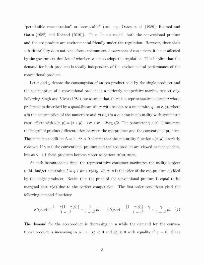
present our numerical illustration in a dynamic setting. A series of Figures 4 to 9 shows the six

trajectories of the equilibrium paths, which respectively represent the six scenarios. Figures

4 to 9 respectively correspond to the marginal cost of the eco-product; the eco-product price;

consumer surplus; the profit for the eco-product producers; the negative externalities; and

social welfare, as shown in the captions.

We now characterize the impact of the regulation on social welfare along the equilibrium

path converging to the steady state (Figure 9) by examining each of the two components of

social welfare: total surplus (consumer surplus plus the profit for the single producer) and

the negative externalities.19 Concerning total (consumer) surplus as the first component,

notice that the regulation triggers innovation of the eco-product technology so that it lowers

the equilibrium path of the marginal cost (Figure 4). When the degree of dynamic learning

effect is high, the regulation enhances learning so that it lowers the equilibrium path of the

19In our numerical examples, the profit for the single producer is relatively small compared to consumersurplus and can be considered negligible. Thus, the discussions on consumer surplus is almost equivalent tothose on total surplus.

27

price of the eco-product (Figure 5). In this case, under the regulation, the negative impact

on consumer surplus associated with the rise in the conventional product price would be

recovered over time as the price of the eco-product falls over time (see the trajectories of

{(NR,H), (R,H)} in Figure 6). However, the regulation does not always cause total (con-

sumer) surplus in later periods to go over the level achieved under non-regulation. Indeed,

when the degree of dynamic learning effect is small, the regulation fails to make the pricing

schedule sufficiently low and total (consumer) surplus in later periods cannot reach the level

under non-regulation (see the trajectories of {(NR,M), (R,M)} and {(NR,L), (R,L)} in

Figures 5 and 6).20 Taking into account that the current value of the regulation over time

is highly concerned with the dynamic trade-off between the steady-state outcome and the

initial loss in early periods, the above discussions could imply that the current value of the

regulation over time related to total (consumer) surplus is likely to be increasing in the

degree of dynamic learning effect. This feature is the same as the one associated with total

surplus in the steady state as proven in Proposition 4, however, it is again in sharp contrast

with the static case.

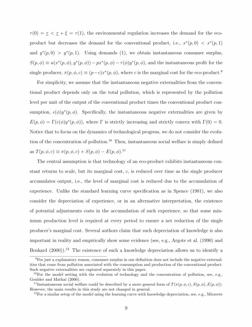
Regarding the negative externalities as the second component, the current value of reg-

ulation over time related to the negative externalities would be decreasing in the degree

of learning as illustrated in Figure 8. Since we assume that the regulation removes the

negative externalities, only three trajectories of {(NR,L), (NR,M), (NR,H)} are drawn in

that figure. A higher degree of dynamic learning effect intensifies the promotion of the eco-

products and thus reduces the negative externalities along all the equilibrium path under

non-regulation. Thus, the current value of the regulation over time related to the negative

externalities also becomes less as the degree of dynamic learning effect is larger.

20Figures 4 reveals that for any degree of dynamic learning effect, the equilibrium path of the marginalcost under the regulation, denoted by (R, j), j = {L,M,H}, is lower than that under non-regulation (NR, i)over all the equilibrium path. (Here it must be noted that although two trajectories of (NR,L) and (R,L)cannot be distinguished, (R,L) is lower than (NR,L) as in the other case). However, by observing thetrajectories of (R,L) and (NR,L) in Figure 5, we notice that the equilibrium path of the eco-product priceunder the regulation may be higher than that under non-regulation if the degree of dynamic learning effectis small. In this case, the situation is very close to the static case, and thus the pricing schedule under theregulation may be higher.

28

We can summarize the impacts of the regulation on each component of social welfare at

this point. There are potentially two different consequences on total (consumer) surplus and

the negative externalities between the static and the dynamic models. First, as in the static

model, the regulation in the dynamic model also has a potential adverse effect on consumer

surplus especially in early periods for any degree of dynamic learning effect (see Figure 6).

However, the crucial distinction between the static model and the dynamic model is that

in the dynamic model, the regulation might offset such a negative impact with a potential

future gain through a decline in the price of the eco-product when the degree of dynamic

learning effect is sufficiently high. This implies that learning has a positive impact on the

current value of the regulation. Second, as the degree of dynamic learning effect is larger, the

negative externalities are endogenously reduced more effectively even without the regulation.

Thus, learning has a negative impact on the current value of the regulation, in contrast to

the first. However, such two dynamic impacts do not exist at all in the static model.

Combining the impacts of the regulation on the above two components of social welfare,

we can conclude that the current value of the regulation over time related to the negative

externalities works in the opposite direction with that related to total (consumer) surplus as

the degree of dynamic learning effect changes. This situation is quite similar to that in the

steady state outcome as shown in Proposition 4, where the value of the regulation related to

total (consumer) surplus in the steady state is increasing and that related to environmental

damages in the steady state is decreasing in the degree of dynamic learning effect. Thus, the

U-shaped property could also be expected for the current value of the regulation.

Figure 10 illustrates the graph of the current value of the regulation as a function of

the degree of dynamic learning effect with an initial marginal cost c0 = 0.77 as given. It

confirms that the current value of the regulation holds a non-monotone U-shaped feature,

and that there may be a certain range of λ such that the current value of the regulation

is negative. This result implies that the optimal decision of the regulation in a dynamic

setting could be converse to that of a static setting. In our nemerical example, if the degree

29

of dynamic learning effect is moderate, i.e., λM = 0.18, the current value of the regulation

is negative and the optimal decision of the government is not to adopt the regulation. On

the other hand, if there is no learning, the optimal decision is to adopt the regulation due

to c0 = 0.77 > cM = 0.6816. Therefore, the optimal decision in fact becomes converse.

6 Conclusions

This paper has analyzed the role of the environmental regulation in a situation where an

eco-product newly invented and introduced by a single producer into a market competes

with a pre-existing product supplied under perfect competition due to their substitutability.

Both a static model and a dynamic model have been examined analytically or numerically

when a social planner has an option of tightening the environmental regulation to improve

social welfare. An essential feature of our dynamic model is learning-by-doing technology in

an eco-product planning. We characterize the situation under which the government should

adopt the regulation and discussed how learning-by-doing affects the optimal decision of the

government.

The research shows that in the static setting without learning effect, the regulation should

be adopted if the marginal cost of the eco-product production is high enough, and otherwise

it should not. On the other hand, in the dynamic model with learning effect, whether or not

the regulation improves social welfare is highly dependent not only on the current marginal

cost of the eco-product but also on the degree of dynamic learning effect. These bear some

resemblance with the general result from Baumol and Oates (1988) that the environmental

regulation should be less stringent under imperfect competition.

In particular, using numerical analysis, this study illustrates an interesting and plausible

case where the regulation improves social welfare when learning effect is either small or large

enough, while it reduces social welfare in an intermediate range. The current value of the

regulation could possess a nonmonotone U-shaped feature with respect to learning effect.

30

Furthermore, the comparison of static and dynamic cases offers some insight on the optimal

decision made by the central authority and suggests that the optimal decision in a static

case could be in stark contrast to that in a dynamic case under certain conditions.

This provides important policy implications since the existence of learning potentials

could significantly affect the optimal deicision as well as the resulting social welfare. The

regulation enhances technological progress and partially plays the similar role of a rise in

the degree of learning effect. However, it does not always guarantee that such technological

progress induced by the regulation brings about favorable outcomes on social welfare. This

implies that if the government does not consider learning in an eco-product planning, the

regulation may yield unexpected loss in social welfare. Therefore, the government needs to

carefully evaluate learning potentials when the regulation is determined.

There are several additional topics that were not addressed in this paper but can be ex-

amined in the future. First, one potential issue is how incentive schemes such as subsidy/tax

imposed by the government affect the promotion of the eco-product as well as social welfare

in an economy where the eco-product whose technology entails learning is differentiated from

the conventional polluting product. Second, the role of research and development should also

be examined in the similar situation since it has been widely considered another engine of

technological progress in terms of not only process innovation but also product innovation.

Third, more importantly, loosening some restrictions on the choice of the regulation placed

in this paper would enable us to derive some important results. For example, instead of a

binary choice of the regulation, analyzing a continuous standard could help us examine how

the optimal standard depends on the degree of dynamic learning effect.

As another future research topic, we are especially interested in the case where the

government can change the standard within his discretion. This seems to be somewhat

concerned with the problems of time-consistency that has been actively addressed in the other

field of economics. In this case, the dynamic strategic interaction between the government

and the industry would be crucial in characterizing the equilibrium outcomes. These caveats

31

notwithstanding, we believe that the basic structure of the model introduced in this paper

would be a first step towards exploring some fuller models to addressing further issues as

listed above. We are hopeful that the results of our research clarify the potential effects of

tightening environmental regulation so as to promote eco-products in the presence of learning

effect, and stimulate the further research questions.

7 Appendix

For some preliminary purposes, we first derive some important variables in the case of staticpricing of the eco-product. Using (3), we obtain xM(φ, c) = 1−c−γ(1−τ(φ))

2(1−γ2)> 0, yM(φ, c) =

(1−τ(φ))(2−γ2)−γ(1−c)2(1−γ2)

> 0, and πM(φ, c) = [1−c−γ(1−τ(φ))]2

4(1−γ2). Moreover, using (3), we obtain

EM(φ, c) = Γ(εyM(0, c)) if φ = 0 and EM(φ, c) = 0 if φ = 1.

Claim 1 For any φ ∈ {0, 1}, technological progress in the production of the eco-product (1)decreases the optimal eco-product price; (2) increases the output of the eco-product; (3) de-creases the output of the conventional product and the negative externalities; and (4) increasesconsumer surplus as well as the profit for the single producer.

Proof of Claim 1 Differentiating pM , xM and yM with respect to c yields ∂pM∂c

= 12> 0;

∂xM∂c

= − 12(1−γ2)

< 0; and ∂yM∂c

= γ2(1−γ2)

> 0, which are the desired results in (1), (2)

and (3). Noticing that ∂S∂p

= (ux − p)∂x∗

∂p+ (uy − τ(φ))∂y

∗

∂p− x∗ = −x∗ < 0 and that

xM(φ, c) > 0 or 1− c− γ(1− τ(φ)) > 0, we obtain ∂SM

∂c= ∂S

∂p∂pM∂c

= −xM(φ, c)∂pM∂c

< 0 and∂πM∂c

= −1−c−γ(1−τ(φ))2(1−γ2)

< 0, which are the desired results in (4). �

Proof of Proposition 1 Let p(ξ, c) ≡ pM(1, c : ξ), x(ξ, c) ≡ xM(1, c : ξ), y(ξ, c) ≡ yM(1, c :ξ), S(ξ, c) ≡ SM(1, c : ξ), and π(ξ, c) ≡ πM(1, c : ξ). Notice that pM(0, c) = p(0, c),xM(0, c) = x(0, c), yM(0, c) = y(0, c), SM(0, c) = S(0, c), and πM(0, c) = π(0, c). Since∂p∂ξ

= γ2> 0, it must hold that pM(0, c) = p(0, c) < p(ξ, c) = pM(1, c : ξ) for any ξ > 0,

which is the desired result in (1). Similarly, since ∂x∂ξ

= γ2(1−γ2)

> 0 and ∂y∂ξ

= − 2−γ22(1−γ2)

< 0,

it must hold that xM(0, c) = x(0, c) < x(ξ, c) = xM(1, c : ξ) and yM(0, c) = y(0, c) >y(ξ, c) = yM(1, c : ξ) for any ξ > 0, which are the desired results in (2). Moreover, notice

that ∂S∂ξ

= [ux − p]∂x∂ξ

+ [uy − (τ + ξ)]∂y∂ξ− x∂p

∂ξ− y = −x∂p

∂ξ− y < 0. Thus, it must hold

that SM(0, c) = S(0, c) > S(ξ, c) = SM(1, c : ξ) for any ξ > 0, which is the desired result in

the first part of (3). Since ∂π∂ξ

= γ[1−c−γ(1−τ−ξ)]2(1−γ2)

> 0, it must hold that πM(0, c) = π(0, c) <

π(ξ, c) = πM(1, c : ξ) for any ξ > 0, which is the desired result in the second part of (3). �

Proof of Proposition 2 Note ∆TM(c) = T (pM(1, c), 1, c)−T (pM(0, c), 0, c) = Γ(εyM(0, c))+

Φ(ξ, c), where Γ(εyM(0, c)) = Γ(ε (1−τ)(2−γ2)−γ(1−c)2(1−γ2)

) and Φ(ξ, c) = (SM(1, c) + πM(1, c)) −(SM(0, c) + πM(0, c)). For any ε, Γ(εyM(0, c)) is increasing and convex in c since ∂Γ

∂c=

32

Γ′(εyM)ε∂yM∂c

> 0 and ∂2Γ∂c2

= ε[Γ′′(εyM)ε(∂yM∂c

)2+ Γ′(εyM)∂

2yM∂c2

] > 0. Moreover, Φ(ξ, c) is

strictly decreasing in c with linearity since ∂Φ(ξ,c)∂c

= − 3γξ4(1−γ2)

< 0. Taking into account that

∆TM(0) < 0 and ∆TM(1) > 0 and that Γ is increasing and convex, it must hold that thereexists a unique critical value cM > 0 such that Φ(ξ, c) > −Γ(εyM(0, c)) or T (pM(1, c), 1, c) >T (pM(0, c), 0, c) if c > cM and Φ(ξ, c) < −Γ(εyM(0, c)) or T (pM(1, c), 1, c) < T (pM(0, c), 0, c)if c < cM . �

Claim 2 The critical value cM is decreasing in the pollution level per unit of the output ofthe conventional product, ε. Furthermore, the critical value cM is increasing in the effect ofthe regulation on the marginal cost of the conventional product, ξ.

Proof of Claim 2 Notice that ∆TM(c) = Φ(ξ, c) + Γ(εyM(0, c)) = 0 is increasing in c inthe neighborhood of c = cM(ξ, ε). This implies that at c = cM(ξ, ε), Γ′(εyM)ε∂yM

∂c+ ∂Φ

∂c> 0.

Differentiating ∆TM(cM(ξ, ε)) = Φ(ξ, cM(ξ, ε)) + Γ(εyM(0, cM(ξ, ε))) = 0 with respect to ε

yields ∂cM (ξ,ε)∂ε

= −Γ′(εyM)yM [Γ′(εyM)ε∂yM∂c

+ ∂Φ∂c

]−1 < 0 since Γ′(εyM)ε∂yM∂c

+ ∂Φ∂c

> 0 andΓ′ > 0. Thus, cM(ξ, ε) is decreasing in ε. Furthermore, differentiating ∆TM(cM(ξ, ε)) = 0

with respect to ξ yields that ∂cM (ξ,ε)∂ξ

= −∂Φ∂ξ

[Γ′(εyM)ε∂yM

∂c+ ∂Φ

∂c

]−1> 0 ⇔ ∂Φ

∂ξ< 0. Thus,

cM(ξ, ε) is increasing in ξ. �

Claim 3 For any φ ∈ {0, 1}, there exists a unique steady state (c(φ), p(φ)). Furthermore,the unique steady state is stable if the degree of product differentiation between the eco-product and the conventional product is small enough so that det(M) < 0 or γ < γ, whereγ ≡ (1− r+2λδ

2δ(r+λδ))1/2.

Proof of Claim 3 Since the system (4) is a linear differential system, the desired result inthe first part is directly obtained. The proof of the second part follows Kamien and Schwartz(2012). The characteristic equation associated with (4) is k2− rk−λδ(r+λδ) + (r+2λδ)λ

2(1−γ2)= 0

with roots k1, k2 = r2± 1

2[(r+2λδ)2− 2λ(r+2λδ)

1−γ2 ]1/2 ≡ r2± 1

2D1/2. Then, the solution has the form

of c(t) = Aek1t + Bek2t for k1, k2 real and distinct, or c(t) = (A + Bt)ert/2 if k1 = k2 = r/2,or c(t) = ert/2(A cos pt + B sin pt), where p = (−D)1/2, if p is real. If the roots are real, thelarger root must be positive. The smaller root may be either positive or negative. It willbe negative if r < D1/2; that is if δ(r + λδ) > r+2λδ

2(1−γ2)or γ2 < 1 − r+2λδ

2δ(r+λδ)≡ γ2, the roots

are real and of opposite signs. Let k1 > 0 > k2 if γ2 < γ2 holds. Then, c(t) will convergeto zero provided we take A = 0. Thus, if γ2 < γ2 holds, then the roots must be real andthe steady state must satisfy the conditions to be a saddlepoint. On the other hand, theroots will be real and nonnegative if D ≥ 0 and γ2 < γ2 fails. As long as the roots are bothnonnegative, c(t) cannot converge to the steady state. It will move away from it, unless theinitial position happens to be the steady state. Finally, the roots will be complex if D < 0.Note that since the real part of the complex roots is positive (= r/2), the path moves awayfrom the steady state so that the steady state is unstable. In sum, a solution to the system(4) can converge only if γ2 < γ2 holds. In other cases, all paths diverge. �

Claim 4 For any φ, if λ > 0 and γ < γ, in the steady state, an increase in λ (1) reducesthe marginal cost and the price of the eco-product; (2) raises the output of the eco-product;(3) reduces the output of the conventional product and the negative externalities; and (4)increases consumer surplus.

33

Proof of Claim 4 By equation (6), we obtain xM(φ, c(φ)) = σ(c(φ))[1− λ2(r+λδ)(1−γ2)

]. We

first show ∂c∂λ< 0. Differentiating this with respect to λ yields ∂c(φ)

∂λ= − rσ(c)

2(r+λδ)2(1−γ2)[∂xM∂c−

∂σ∂c

(1 − λ2(r+λδ)(1−γ2)

)]−1. Notice that since γ < γ, we obtain ∂xM∂c− ∂σ

∂c(1 − λ

2(r+λδ)(1−γ2)) =

− δ1−γ2 [γ2 − (1 − r+2λδ

2δ(r+λδ))] > 0. Thus, we obtain ∂c

∂λ< 0, which is the desired result in the

first part of (1). Note that p(φ) = pM(φ, c(φ))− λσ(c(φ))2(r+λδ)

. Differentiating this with respect to

λ yields ∂p(φ)∂λ

= ∂pM∂c

∂c∂λ− 1

2[ rσ(c(φ))

(r+λδ)2− λδ

r+λδ∂c∂λ

]. Since ∂pM∂c

> 0 and ∂c∂λ< 0, it must hold that

∂p(φ)∂λ

< 0, which is the desired result in the second part of (1). We then show that ∂x∂λ> 0

and ∂y∂λ< 0, which are the desired results in (2) and (3). By equation (1), the outputs of the

eco-product and the conventional product in the steady state are given by x(φ) = x∗(p(φ), φ)

and y(φ) = y∗(p(φ), φ), which implies that ∂x(φ)∂λ

= ∂x∗

∂p∂p(φ)∂λ

= − 11−γ2

∂p(φ)∂λ

> 0 and ∂y(φ)∂λ

=∂y∗

∂p∂p(φ)∂λ

= γ1−γ2

∂p(φ)∂λ

< 0. We next show that ∂S(φ)∂λ

> 0, which is the desired result in (4).

Using S(φ) = S(p(φ), φ), ∂p∂λ< 0 and ∂S

∂p= −x(φ), we obtain ∂S(φ)

∂λ= ∂S

∂p∂p∂λ

= −x(φ) ∂p∂λ> 0.

�

Proof of Proposition 3 Since γ > γ, it must hold that ∆c ≡ c(0)− c(1) > 0, which is the

desired result of the first part. Moreover, since ∂γ∂λ< 0, it must hold that ∂(∆c)

∂λ> 0, which is

the desired result of the second part. �

References

Ambec, S., Cohen, M. A., Elgie, S., and Lanoie, P. (2013). The Porter hypothesis at20: Can environmental regulation enhance innovation and competitiveness? Review ofenvironmental economics and policy, 7:2–22.

Argote, L., Beckman, S. L., and Epple, D. (1990). The persistence and transfer of learningin industrial settings. Management science, 36(2):140–154.

Argote, L. and Epple, D. (1990). Learning curves in manufacturing. Science, 247(4945):920–924.

Arora, S. and Gangopadhyay, S. (1995). Toward a theoretical model of voluntary overcom-pliance. Journal of environmental economics and management, 28:289–309.

Arrow, K. J. (1962). The economic implications of learning by doing. Review of economicstudies, 29:155–173.

Bansal, S. and Gangopadhyay, S. (2003). Tax/subsidy policies in the presence of environmen-tally aware consumers. Journal of environmental economics and management, 45:333–355.

Baumol, W. J. and Oates, W. E. (1988). The theory of environmental policy. Cambridgeuniversity press, 2 edition.

Bellas, A. S. (1998). Empirical evidence of advances in scrubber technology. Resource andenergy economics, 20:327–343.

34

Benkard, C. (2000). Learning and forgetting: The dynamics of aircraft production. Americaneconomic review, 90(4):1034–1054.

Besanko, D., Doraszelski, U., and Kryukov, Y. (2014). The economics of predation: Whatdrives pricing when there is learning-by-doing. American economic review, 104:868–897.

Conrad, K. (2005). Price competition and product differentiation when consumers care forthe environment. Environmental and resource economics, 31:1–19.

Cremer, H. and Thisse, J. (1999). On the taxation of polluting products in a differentiatedindustry. European economic review, 43:575–594.

Cropper, M. L. and Oates, W. E. (1999). Environmental economics. In Stavins, R. N.,editor, Economics of the environment, selected readings. W. W. Norton & Company, Inc.

Eriksson, C. (2004). Can green consumerism replace environmental regulation?—Adifferentiated-products example. Resource and energy economics, 26:281–293.

Fudenberg, D. and Tirole, J. (1983). Learning-by-doing and market performance. Belljournal of economics, 14:522–530.

Goulder, L. H. and Mathai, K. (2000). Optimal CO2 abatement in the presence of inducedtechnological change. Journal of environmental economics and management, 39:1–38.

Grankvist, G., Dahlstrand, U., and Biel, A. (2004). The impcat of environmental labelling onconsumer preference: Negative vs. positive labels. Journal of consumer policy, 27:213–230.

Greenstone, M. (2003). Estimating regulation-induced substitution: The effect of the cleanair act on water and ground pollution. American economic review, 93(2):442–448.

Jorgenson, D. W. and Wilcoxen, P. J. (1990). Environmental regulation and U.S. economicgrowth. RAND journal of economics, 22:41–69.

Kamien, M. I. and Schwartz, N. L. (2012). Dynamic optimization: The calculus of variationsand optimal control in economics and management. Elsevier North Holland.

Kolstad, C. C. (2010). Environmental economics. Oxford university press, 2 edition.

Loureiro, M. L., Mccluskey, J. J., and Mittelhammer, R. C. (2002). Will consumers pay apremium for eco-labeled apples? Journal of consumer affairs, 36(2):203–219.

Ministry of Environment Government of Japan (2006a). Kankyo Hakusho.

Ministry of Environment Government of Japan (2006b). List of Environmental QaulityStandards in Japan at http://www.env.go.jp/en/standards/.

Miravete, E. J. (2003). Time-consistent protection with learning-by-doing. European eco-nomic review, 47:761–790.

Moraga-Gonzalez, J. L. and Padron-Fumero, N. (2002). Environmental policy in a greenmarket. Environmental and resource economics, 22:419–447.

35

Oates, W. E., Portney, P. R., and McGartland, A. M. (1989). The net benefit of incentive-based regulation: A case study of environmental standard setting. American economicreview, 79(5):1233–1242.

Palmer, K., Oates, W. E., and Portney, P. R. (1995). Tightening environmental standards:The benefit-cost or the no-cost paradigm. Journal of economic perspectives, 9(4):119–132.

Porter, M. E. (1991). America’s green strategy. Scientific american, 264:168.

Porter, M. E. and van der Linde, C. (1995). Toward a new conception of the environment-competitive relationship. Journal of economic perspectives, 9(4):97–118.

Romer, P. M. (1986). Increasing returns and long-run growth. Journal of political economy,94:1002–1037.

Singh, N. and Vives, X. (1984). Price and quantity competition in a differentiated duopoly.RAND journal of economics, 15:546–545.

Spence, M. A. (1981). The learning curve and competition. Bell journal of economics,12:49–70.

Stokey, N. L. (1988). Learning by doing and the introduction of new goods. Journal ofpolitical economy, 96:701–717.

Stranlund, J. K. (1997). Public technological aid to support compliance to environmentalstandards. Journal of environmental economics and management, 34:228–239.

Zhu, J. and Ruth, M. (2015). Relocation or reallocation: Impacts of differentiated energysaving regulation on manufacturing industries in china. Ecological economics, 110:119–133.

36

Figure 1: Phase diagram in marginal cost-price space 0=p& 0=c&

c

p

c p )(ˆ cpp =

0c Figure 2: The value of the regulation ∆T and the degree of dynamic learning effect λ

( )( )0yεΓ

π∆+∆S

T∆

0 1λ 2λ λ

( )( )0yST επ Γ+∆+∆=∆

37

Figure 3: The value of the regulation and the marginal cost of the eco-product (Static Case)

0.1 0.2 0.3 0.4 0.5 0.6 0.7

-0.03

-0.02

-0.01

0

0.01

0.02

0.03

0.04

Marginal cost, c

Value of R

egulation

Figure 4: The marginal cost of the eco-product over time

0 5 10 15 20 25 30

0.2

0.3

0.4

0.5

0.6

0.7

0.8

0.9

Time

Marginal C

ost

(NR,H)

(R,H)

(NR,M)

(R,M)

(NR,L)

(R,L)

38

Figure 5: The price of the eco-product over time

0 5 10 15 20 25 30

0.3

0.4

0.5

0.6

0.7

0.8

Time

Eco-product P

rice

(NR,H)

(R,H)

(NR,M)

(R,M)

(NR,L)

(R,L)

Figure 6: Consumer surplus over time

0 5 10 15 20 25 30

0.1

0.15

0.2

0.25

0.3

Time

Consum

er Surplus

(NR,H)

(R,H)

(NR,M)

(R,M)

(NR,L)

(R,L)

39

Figure 7: The profit of the single producer of an eco-product over time

0 10 20 30

-0.01

-0.005

0

0.005

0.01

0.015

0.02

0.025

0.03

Time

Profit of A

Eco-product P

roducer

(NR,H)

(R,H)

(NR,M)

(R,M)

(NR,L)

(R,L)

Figure 8: The negative externalities over time

0 5 10 15 20 25 30

0

0.01

0.02

0.03

0.04

0.05

0.06

0.07

0.08

Time

Negative Externalities

(NR,H)

(NR,M)

(NR,L)

40

Figure 9: Social welfare over time

0 5 10 15 20 25 30

0.1

0.15

0.2

0.25

0.3

0.35

Time

Social W

elfare

(NR,H)

(R,H)

(NR,M)

(R,M)

(NR,L)

(R,L)

Figure 10: Current value of the regulation over time with the initial marginal cost c0 = 0.77as a function of the degree of dynamic learning effect λ

-0.2-0.100.10.20.30.40.50.60.70.8

0 0.5 1 1.5 2Learning effect

Current vaalue of regulation

41

some implications of environmental regulation on social

Documents