Some examples of Interactive Boundary Layers

P.-Y. LagreeCNRS & UPMC Univ Paris 06, UMR 7190,

Institut Jean Le Rond d’Alembert, Boıte 162, F-75005 Paris, Francepierre-yves.lagree@upmc.fr ; www.lmm.jussieu.fr/∼lagree

September 18, 2009

Abstract

In this chapter we present some other examples of IBL, not only in anaerodynamical context.

1 Introduction

In this chapter we focus on some examples which are not only from theaerodynamical field and which may lead to interacting boundary layer.

It means that we have a kind of Prandtl problem, the external boundaryof it being linked with the variations of velocity or pressure by an exter-nal coupling. To a certain extent the interaction be explained through aretroactive process involving integral concepts as follows: as the variationof pressure is more or less proportional to the variation of the boundarylayer thickness, then the increase of boundary layer thickness promotes arise of pressure, which decreases the velocity, the result is an increase of theboundary layer thickness: the process is self promoting.

First there is the hypersonic problem, this interacting boundary layerflows process was described in Stewartson (1964) [19] with a self inducedmechanism involving variations of boundary layer thickness and pressure.The key mechanism in supersonic and hypersonic flows was introduced byNeiland (1969) [14] and Stewartson & Williams (1969) [20]: it is the ”tripledeck” theory which clarifies the scales and the equations involved in theinteraction. rown, Brown Stewartson & Williams (1975) [5] successfullyexplained the branching solutions calculated in strong hypersonic flows by

1

examples IBL

Werle et al (1973) [22] and the link with Neiland (1970) [15].

Next there is the mixed convection problem. It presented exactly thesame features, and Steinruck (1994) [33]) proposed a kind of branching so-lution and Lagree [31] showed that this may be reformulated in a triple Deckframework.

We present as well equations for the viscous hydraulic jump. The equa-tions for artery flows are of the same vein.

- VI . 2-

examples IBL

2 Hypersonic flows

2.1 Self similar flows

Supersonic and hypersonic flows were developed in the 50’, there was thenover the next 50 years a continuous and sporadic interest linked to theICBML (Intercontinental Ballistic Missiles) and the space conquest fromMoon to Mars via the Space Shuttle. At this early time it was observedthat those flows presented some self similar solutions. In case of negligibleboundary layer thickness, people were looking to power shock laws. In thiscase the body may be a power law shape. This came from the observationthat if we define from the Mach Number M∞ and from the local angle ofthe shock σ and from the slope of the body τ the parameters:

Ks = M∞σ, K = M∞τ

they define self similar parameters in the Hypersonic Small DisturbanceTheory (Chernyi [8]). The oblique shock wave relation gives for small anglesθ and σ :

M∞σ

M∞τ=

γ + 14

+

√(γ + 1

4)2 +

1(M∞τ)2

the pressure is then

p

p∞=

2γ

γ + 1K2

s −γ − 1γ + 1

(1)

= 1 + γγ + 1

4K2 + γK

√(γ + 1

4K)2 + 1. (2)

then for moderate Mach number, we recover that the angle of the shock isa Mach Wave (1/M∞) and the pressure is:

p− p∞ρ∞U2

∞' 1 + Ks

and for a large Mach number the body and the shock are proportional:

M∞σ

M∞τ=

γ + 12

,

and the pressure

p− p∞ρ∞U2

∞' K2

s .

- VI . 3-

examples IBL

Figure 1: Self similar Hypersonic flows from Van Dyke ”An Album of FluidMotion”.

- VI . 4-

examples IBL

As only powers appear, self similar solutions are straightforward. Seefigure 1 for an example extracted from Van Dyke [21].

Those power law were not relevant for all the bodies. One of the selfsimilar solution corresponds to the very special case. This is the blunt bodycase corresponding to a flat plate with a very small nose.

p− p∞ρ∞U2

∞= F (γ)C2/3

d (x/d)−2/3

rshock = G(γ)C1/3d (x/d)2/3

see Guiraud Vallee & Zolver [9], Chernyi [8] and Sedov [18] for details.

2.2 Viscous interaction

For compressible boundary layers, the simple order of magnitude gives:

δ2 =µL

ρU∞

taking into account that the viscosity follows in first approximation theChapman law µ = µ∞C T

T∞and the ideal gaz law: ρ/ρ∞ = (pT )/(p∞T∞),

then:(δ

L)2 ∼ C(

T

T∞)2

p∞p

1R∞

• In the so called ”weak hypersonic interaction” pressure remains oforder p∞ and the temperature ratio is of order of order M2

∞so that:

(δ

L) ∼ C1/2(

T

T∞)

1

R1/2∞

=χ∞M∞

were χ∞ = C1/2 M2∞

R1/2∞

is the hypersonic parameter. The pressure is then:

p− p∞ρ∞U2

∞' 1 + χ∞

• In the so called ”strong hypersonic interaction” pressure is now deter-mined bay the equivalent body which is the displacement thickness due tothe strong viscous effects.

p

p∞' K2 with K = M∞(δ/L).

so wee obtain the displacement thickness as:

δ

L∼

√1

M∞χ∞,

p

p∞' χ2

∞

this represents a shock and a boundary layer in x3/4.

- VI . 5-

examples IBL

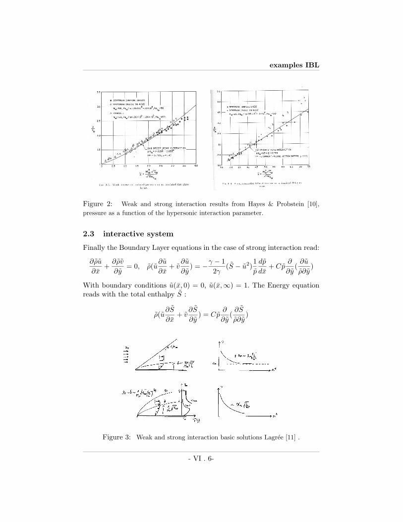
Figure 2: Weak and strong interaction results from Hayes & Probstein [10],pressure as a function of the hypersonic interaction parameter.

2.3 interactive system

Finally the Boundary Layer equations in the case of strong interaction read:

∂ρu

∂x+

∂ρv

∂y= 0, ρ(u

∂u

∂x+ v

∂u

∂y) = −γ − 1

2γ(S − u2)

1p

dp

dx+ Cp

∂

∂y(

∂u

ρ∂y)

With boundary conditions u(x, 0) = 0, u(x,∞) = 1. The Energy equationreads with the total enthalpy S :

ρ(u∂S

∂x+ v

∂S

∂y) = Cp

∂

∂y(

∂S

ρ∂y)

Figure 3: Weak and strong interaction basic solutions Lagree [11] .

- VI . 6-

examples IBL

The boundary layer displacement thickness gives the velocity at the edge ofthe boundary layer as

ve(x) =d

dx[γ − 12p

∫ ∞

0(S − u2)ρy]

and the coupling relation is:

p =γ + 1

4v2e .

This interactive system was believed to be solved with a marching scheme.But, unfortunately it raised difficulties, one observed branching solutionwhen solving numerically for increasing x (see Neiland [15] and figure 6right thereafter, see Werle et al. [22]... and figure 4).

Figure 4: Branching solutions [22]: changing a bit one parameter may causedifferent solutions while solving the equations with a marching scheme.

2.4 Hypersonic Triple Deck Stewartson

From this system Stewartson [5] obtained the p = −A relation, this comesfrom the solution of the total enthalpy in the main deck which is obtainedfrom S = S(Y ) + εA(x)S′(Y ) and u = UB(Y ) + εA(x)U ′

B(Y ). It is substi-tuted in the coupling relation for a short disturbance in longitudinal scale:

p =γ + 1

4(γ − 12p

∫ ∞

0(S − u2)ρy)2.

which gives −A contribution in the integral and the development of 1p gives

−p so that the RHS is (−p − A)′ with the ad hoc scales. The case of verycold walls sw << 1 or ”Newtonian flow” (γ close to 1) gives then p = −A.The moderate case is then:

µp = −p′ −A′, with µ ∼ (γ − 1)2s6w.

- VI . 7-

examples IBL

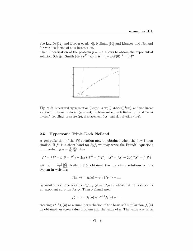
See Lagree [12] and Brown et al. [6], Neiland [16] and Lipatov and Neilandfor various forms of this interaction.Then, linearisation of the problem p = −A allows to obtain the exponentialsolution (Gajjar Smith [49]) eKx with K = (−3Ai′(0))3 = 0.47

0

1

2

3

4

5

6

7

8

-30 -20 -10 0 10 20 30

xtilde

-Ap

exp.tau

Figure 5: Linearized eigen solution (”exp.” is exp((−3Ai′(0))3)x)), and non linearsolution of the self induced (p = −A) problem solved with Keller Box and ”semiinverse” coupling: pressure (p), displacement (-A) and skin friction (tau).

2.5 Hypersonic Triple Deck Neiland

A generalization of the FS equation may be obtained when the flow is nonsimilar. If f is a short hand for ∂xf , we may write the Prandtl equationsin introducing n = x

ue

duedx then

f ′′′ + ff ′′ − β(S − f ′2) = 2x(f ′f ′ − ff ′′), S′′ + fS′ = 2x(f ′S − fS′)

with β = γ−1γ

xdppdx . Neiland [15] obtained the branching solutions of this

system in writting:

f(x, η) = f0(η) + φ(x)f1(η) + ....

by substitution, one obtains F (f0, f1)φ = xdφ/dx whose natural solution isan exponent solution for φ. Then Neiland used

f(x, η) = f0(η) + xa+1f1(η) + ....

treating xa+1f1(η) as a small perturbation of the basic self similar flow f0(η)he obtained an eigen value problem and the value of a. The value was large

- VI . 8-

examples IBL

Figure 6: Left: Pressure at separation point far from the cause, showing com-parisons with experiments supersonic case Neiland (1969) [14]. Right branchingsolution for the hypersonic solution by Neiland (1970) [15]

49.6 for sw = 1. Latter Brown and Williams [7] looked at this same problemwith the same point of view but do not restrict to sw = 1.

We have already mentioned that supersonic flows presented ”upstreaminfluence”. It meant that disturbances have an influence far upstream whichwas a paradox due to the hyperbolic nature of the Euler equations and tothe parabolic nature of the boundary layer equations.

2.5.1 Hypersonic Triple Deck Neiland-Stewartson

What is strange is that two points of view gave different results for the sameset of equations. Stewartson made a local analysis at a small scale and ob-tained eigen solution in exponential. Neiland did not change the longitudinalscale, he obtained power law solution with a large value of the exponent.

Stewartson (Brown Stewartson & Williams [5]) reconciled the two pointsof view in noting the link between the two results (algebraic and exponen-

- VI . 9-

examples IBL

tial). He observed that far upstream near a given X0, one can do a localstudy at scale x3 so that

x = x0 + x3x

the power law behaviour is :

(x)n = enLog(x0(1+x3x/x0)) ' enLog(x0)ex3x/x0

so in the local variables algebraic behaviour looks like an exponential.

- VI . 10-

examples IBL

3 Heat Flows

Flow with temperature are good candidates to coupling in the case of mixedconvection. It means that there is a basic stream which imposes forced con-vection but it means that there is some natural convection as well creatinga retroaction. We will see what happens for plumes en jets and in the caseof mixed convection.

3.1 The mixed convection problem

Here we consider first the mixed convection problem of an incompressiblebuoyant (following the Boussinesq approximation) fluid flowing over a semiinfinite horizontal flat plate at a constant temperature lower than the in-coming flow temperature (see figure 7 for a definition sketch). Obviously,for a given x location, the fluid temperature, by diffusion, increases fromthe wall value towards that of the free stream. But for a fixed y location theconvection induces a longitudinal decrease of the temperature. The outcomeis a buoyancy induced stream wise adverse pressure gradient. This gradientbrakes the flow, and this creates an interaction between the thermics and thedynamics. This mechanism of mixed convection breakdown has been statedby Schneider & Wasel (1985) [32] (other examples of re-computation withdifferent numerical methods are reviewed by Steinruck (1994) [33]); theyshowed that this interaction promotes a breakdown of the mixed boundarylayer equation: at a relatively small abscissa, the equations are abruptlysingular. Instead of a buoyant boundary layer a buoyant wall jet may bestudied, the case of adiabatic wall was studied by Daniels (1992) [25] andDaniels & Gargaro (1993) [26], they found the same conclusions. The walljet problem is solved numerically and asymptotically by Higuera (1997) [51]who notes that the equations are not parabolic as he noted before in thecase of the hydraulic jump which is very similar in its behaviour.

3.2 Governing equations of the mixed convection

3.2.1 Equations

We consider an incompressible two dimensional flow past a semi-infinite(heated or cooled) horizontal flat plate (figure 7). The boundary layerequations are obtained from the Navier Stokes counter parts subject toBoussinesq approximation for a large Reynolds number. A re-scaling ofthe dimensional quantities is carried out with the dynamical boundary layer

- VI . 11-

examples IBL

Figure 7: Sketch of the mixed convection boundary layer flow, the temperatureof the plate is different from the temperature of the flow. If the plate is cooled, thebuoyancy induces an adverse pressure gradient.

scales (with δ = Re−1/2 with Re = ρ∞U∞L/µ):

u∗ = U∞u, v∗ = δU∞v,x∗ = Lx, y∗ = δLy,p∗ = p∞ + ρ∞U2

∞p, T = T∞ + (T0 − T∞)θ,

the result is the classical system (23- 7) of thermal mixed convection (Schnei-der & Wasel (1985) [32]), Prandtl number is assumed to be of order unityand hence set, (without to much loss of generality), to one while the Eckertnumber is assumed sufficiently small to obtain the energy equation as (7)).The remaining parameter is the Richardson number or buoyancy parameter:

J =αg(T0 − T∞)LRe−1/2

U2∞

, (3)

it depends on α the thermal coefficient of expansion of the density in theBoussinesq approximation. The transverse pressure term (6) contains thegravity term, as equation (6) holds for terms greater than O( 1

Re), we have|J | >> Re−1:

∂

∂xu +

∂

∂yv = 0, (4)

u∂

∂xu + v

∂

∂yu = − ∂

∂xp +

∂2

∂y2u, (5)

0 = − ∂

∂yp + Jθ, (6)

- VI . 12-

examples IBL

u∂

∂xθ + v

∂

∂yθ =

∂2

∂y2θ, (7)

Boundary conditions are:

u(x, y = 0) = 0, v(x, y = 0) = 0, (8)

θ(x, y = 0) = θw with θw = 1, u(x, y −→ ∞) = 1, θ(x, y −→ ∞) =0, p(x, y −→∞) = 0.

3.2.2 Marching breakdown

The length scale L and the parameter J are independent, it contrasts withthe situation in Schneider & Wasel (1985) [32] or in Daniels & Gargaro(1993) [26]. In the ”real mixed convection problem with stable stratificationflow”, the ”natural” longitudinal scale is effectively built with Richardsonnumber. It is the length that gives unit Richardson number(∣∣αg(T0 − T∞)LT U−2

∞ (U∞LT ν−1)−1/2∣∣ = 1), so:

LT =U∞ν

(U2∞

−αg(T0 − T∞))2.

Note that J2LT = L. Schneider & Wasel (1985) [32] (scaled with LT ) showedthat this system leads to a singularity when solved with a marching (inincreasing x) resolution. They showed that the breakdown occurs for arather small abscissa. This is the reason why Steinruck (1994) [33] (scaledwith LT ) has investigated how the system (23-7) behaves when x tendsto 0. In figure 8 are displayed, with symbols, the reduced skin frictionfrom previous works compiled by Steinruck. The curves with numbers showsolution of the marching problem with slightly perturbed initial conditionsand come from his analysis near x = 0. Asymptotic analysis suggests,however, that it is better to consider an intermediate scale L (with L << LT )leading to Blasius boundary layer (with this scales x tends to 0 is the noseeffect) with a small thermal perturbation gauged by |J | << 1, this meansthat the Richardson number built with this abscissa is smaller than one. So,we will introduce the triple deck analysis.

- VI . 13-

examples IBL

Removing the marching breakdown of the boundary-layerequations for mixed convection above a cooled horizontal plate

Pierre-Yves LagreeLaboratoire de Modelisation en Mecanique

Universite PARIS VI, FRANCEEmail: pyl@ccr.jussieu.fr

Keywords - Interacting Boundary Layer - Mixed convection - Triple Deck

Abstract -The thermal mixed convection boundary-layer flow over a flat horizontal cooled plateis revisited. Written in boundary layer notations, the system to solve is:

!

!xu +

!

!yv = 0, u

!

!xu + v

!

!yu = !

!

!xp +

!2

!y2u, (1)

0 = !!

!yp + J", u

!

!x" + v

!

!y" =

!2

!y2". (2)

Boundary conditions are: (u(0, y) = 1, v(0, y) = 0, "(0, y) = 0), (u(x, 0) = 0, v(x, 0) = 0, "(x, 0) =1), and (u(x,") = 1, "(x,") = 0, p(x,") = 0). The parameter J gauges the e!ect of the buoy-ancy. If this system is solved with a marching in x procedure in the cooled wall case (J < 0),branching solutions appear (left fig.).

-0.05

0

0.05

0.1

0.15

0.2

0.25

0.3

0.35

0 0.05 0.1 0.15 0.2 0.25 0.3

marching5102050100125

f”(

#,0)

#

-0.05

0

0.05

0.1

0.15

0.2

0.25

0.3

0.35

0 0.05 0.1 0.15 0.2 0.25 0.3

marching5102050100125

f”(

#,0)

#

The reduced skin friction f”(#, 0) = !u!y (x, 0)

#x function of # = |J |

#x: marching computations

(Steinruck JFM 278 (1994)) (left) and numerical resolution showing the reverse flow, eachcurve is associated with di!erent domain length xout (right).

The observed singular solutions which branch out may then be revisited in the framework of the“triple deck” theory: two salient structures emerge, one in double deck, if |J | << 1, and another

Figure 8: the reduced skin friction f”(ξ, 0) = ∂u∂y (x, 0)

√x function of ξ = |J |

√x:

compiled and computed by marching computations by Steinruck (JFM 94), thenumbered curves show solution of the marching problem with slightly perturbedinitial conditions (left). Numerical resolution showing the reverse flow, each curveis associated with different domain length xout (right) by Lagree [31].

- VI . 14-

examples IBL

Hypersonique/ Thermique

commercial FLUENT. C’est ce que l’on observe sur la figure 2. A gauche sanse!et de gravite, l’e!et d’expansion du chau!age de la plaque du bas deflechitles lignes de courant vers le haut. A droite, l’e!et de la gravite et donc de laconvection mixte fait tomber le fluide froid, on observe les profils de vitesse etla separation (courant de retour) induite sur la paroi du haut.

2.2 Convection thermique mixte sur une plaque plane ho-rizontale froide [3], [4], [5], [10], [11], [8]

Le cas de convection thermique mixte academique est examine.Comme on l’a deja dit, lorsqu’un fluide s’ecoule sur une plaque plane hori-

!"#$%%&#'&()%$$

*

!" #$%#&' () *+& ()*&,-.*($)/ 0,$1)2 3*&1-,*4$) -)' 5(%6!! %(-74 89:2 -)' 0,$1) -)' 3*&1-,*4$) 8!: 4;..&44<;%%=!9 &>?%-()&' *+& @,-).+()A 4$%;*($)4 .-%.;%-*&' () 4*,$)A!B +=?&,4$)(. C$14 @= 5&,%& &* -%/ 8D!: -)' *+& %()E 1(*+!F G&(%-)' 8H": I*+(4 (4 - <,&& .$)#&.*($) +=?&,4$)(.9J @$;)'-,= %-=&, 1+&,& *+& 4+$.E -)' *+& @$;)'-,= %-=&,9K @&+-#& () !L!DM/ 3().& @$*+ *+& 7&.+-)(47 $< NN*+&,7-%9H 7(>&' .$)#&.*($) 1(*+ %$1 1-%% *&7?&,-*;,&OO -)' $< *+&9L NN4*,$)A%= ()*&,-.*()A +=?&,4$)(. @$;)'-,= %-=&,OO 4&&79D *$ <$%%$1 P;-%(*-*(#&%= *+& 4-7& ?-*+2 1& ?,$?$4& *$9" ,&#(4(* *+& 7(>&' .$)#&.*($) 1(*+ *+& *,(?%& '&.E *$$% I4&&9! 8L": <$, $*+&, &>-7?%&4M/99 Q+&,7-% &R&.*4 () @$;)'-,= %-=&, 1(*+ *,(?%& '&.E9B +-#& @&&) -%,&-'= 4*;'(&' () *+& .-4& $< 4*,-*(S.-*($) ()9F *+& ;??&, '&.E @= 3=E&4 8DD: -)' 1(*+$;* @;$=-).= @=BJ T&)'&U &* -%/ 8HD: $, $) - #&,*(.-% ?%-*& @= V% W-S 8KH:/BK 3$7& *,(?%& '&.E () 7(>&' .$)#&.*($) (4 () 8KF:2 -)' (4BH &>*&)'&' +&,&()/BL X) *+(4 ?-?&, 1& 4&& I3&.*($) L/KM *+-* *+& ,&4;%* $< *+&BD *,(?%& '&.E *+&$,= (4 *+-*2 () - 7(>&' *+&,7-% %()&-,(U&'B" @$;)'-,= %-=&, I.$%' 1-%% 1(*+ #&,= 47-%% @;$=-).= " M2B! *+&,& &>(4* &(A&) 4$%;*($)4 1+&,& ?,&44;,& (4 ?,$?$,*($)-%B9 *$ *+& '(4?%-.&7&)* $< *+& 4*,&-7%()&4Y *+(4 (4 %(E& *+&BB @(,*+ $< - +=',-;%(. Z;7? 8L2KL2K!: $, - +=?&,4$)(.BF @$;)'-,= %-=&, 892 KL:/ X) *+& .-4& $< - +$* 1-%%2 ?,&44;,&FJ (4 ?,$?$,*($)-% *$ *+& )&A-*(#& $< *+& '(4?%-.&7&)* $< *+&FK 4*,&-7%()&4 () *+& 7-() ?-,* $< *+& @$;)'-,= %-=&, 1+(.+FH %&-'4 *$ )$ ;?4*,&-7 ()C;&).& @;* *+(4 -??,$-.+ .-?6FL *;,&4 *+& Q$%%7(&) 3.+%(.+*()A 1-#&4 8LD:/ Q+(4 *,(?%&FD '&.E ,&4;%* $< 4*,$)A 4&%<6()';.&' ;?4*,&-7 ()C;&).& 1(%%F" @& 4+$1) *$ @& &>-.*%= *+& &(A&) <;).*($) <$;)' @=F! 3*&(),!;.E 8L9: @;* () *+& %(7(* $< 47-%% " / W& 4+$1&' *+-*F9 47-%% ?&,*;,@-*($)4 <,$7 *+& 4$%;*($) -* - A(#&) %$.-*($)FB I@&<$,& *+& ?,&#($;4%= .$7?;*&' 4()A;%-,(*=M -,& -7?%(6FF S&' &>?$)&)*(-%%=Y 4$ *+& ?$4(*($) $< *+& 4()A;%-,(*= '&6KJJ ?&)'4 4*,$)A%= $) *+& -7?%(S.-*($) $< *+& 47-%%KJK );7&,(.-% &,,$,4/ X<2 *+-)E4 *$ - #&,= ,&S)&' .-%.;%-*($)2KJH *+& @,-).+()A 4$%;*($)4 -,& )$* 4&%&.*&'2 *+& @;$=-).=KJL @&.$7&4 A,&-*&, -)' A,&-*&,/ X< (* (4 $< $,'&, [IKM2 - 4&%<6KJD ()';.&' ()*&,-.*($) (4 -A-() ?$44(@%&2 @;*2 -4 1& 1(%%

KJ"4+$12 -* '(R&,&)* 4.-%&4 I3&.*($) L/HM/ X) *+(4 .-4& *+&KJ!$#&,-%% ?,$.&44 *-E&4 ?%-.& () *+& *+() 1-%% %-=&, (*4&%<KJ9-)' *+&,& (4 )$ ,&*,$-.*($) <,$7 *+& 7-() ?-,* $< *+&KJB@$;)'-,= %-=&, I*+(4 (4 4(7(%-, *$ 1+-* +-??&)4 () ?(?&KJFC$14\ 8HF2LL:M/ Q+(4 4*,;.*;,& (4 4(7(%-, () - .&,*-() 4&)4&KKJ*$ ]-)(&%4 8KJ: -)' *$ 1+-* 3*&(),!;.E 8L9: ,&<&,4 *$ -4 *+&KKKNN$*+&, %-,A& &(A&)#-%;&4OO/ 5& )&>* &>-7()& *+& -@$#&KKH@,&-E'$1) ;4()A ()*&A,-% 7&*+$'4 I3&.*($) DM/ ^ 4$%;6KKL*($) 1(*+ - @-.E C$1 #-%(' -<*&, *+& 4()A;%-, ?$()* (4KKD&>+(@(*&' -)' '(4.;44&'Y %()E4 1(*+ *,(?%& '&.E -)-%=4(4KK"-,& ?,&4&)*&'/KK!_()-%%= I3&.*($) "M2 1& ?,&4&)* - @$;)'-,= %-=&, .-%6KK9.;%-*($) 1(*+ - 4(7?%& S)(*& '(R&,&).& 7&*+$' $< *+&KKB.$7?%&*& ?,$@%&7/ Q$ -#$(' *+& ?,&.&'()A ?,$@%&74KKF;)4*&-'()&44 (4 ()*,$';.&'\ *+& ?%-*& (4 (7?;%4(#&%=KHJ+&-*&' -)' 4*-,*&'/ 5& 1(%% 4&& *+-* - A$$' .+$(.& ()KHK'(4.,&*(U()A *+& %$)A(*;'()-% '&,(#-*(#& () *+& &P;-*($)4KHH-)' - A$$' .+$(.& $< $;*C$1 .$)'(*($)4 ?,&#&)* *+&KHL4?-*(-% 4()A;%-,(*=\ *+(4 -%%$14 *+& @$;)'-,= %-=&, *$KHD4&?-,-*& 1(*+ )&(*+&, &#('&).& $< S)(*& *(7& @,&-E'$1)KH"8D": )$, ()4*-@(%(*(&4/ Q+& 4E() <,(.*($) 1(%% @& 4+$1) *$KH!@& .$+&,&)* 1(*+ 3*&(),!;.EO4 ,&4;%*4 8L9:2 -)' &-.+ $< +(4KH9@,-).+&' 4$%;*($)4 7-= @& ()*&,?,&*&' -4 - 4$%;*($) $< -KHB'$7-() $< '(R&,&)* %&)A*+/

!"#"$ %&'()*+*, (-./0+&*1 &2 03( 4+5(6 7&*'(70+&*

!"#$%!% &'()*+,-.

KLK5& .$)4('&, -) ().$7?,&44(@%& *1$6'(7&)4($)-% C$1KLH?-4* - 4&7(6()S)(*& I+&-*&' $, .$$%&'M +$,(U$)*-% C-*KLL?%-*& I_(A/ KM/ Q+& @$;)'-,= %-=&, &P;-*($)4 -,& $@6KLD*-()&' <,$7 *+& G-#(&,`3*$E&4 .$;)*&, ?-,*4 4;@Z&.* *$KL"*+& 0$;44()&4P -??,$>(7-*($) <$, - %-,A& a&=)$%'4KL!);7@&,/ ^ ,&64.-%()A $< *+& '(7&)4($)-% P;-)*(*(&4 (4KL9.-,,(&' $;* 1(*+ *+& '=)-7(.-% @$;)'-,= %-=&, 4.-%&4KLBI1(*+ ! ! #$"K!H 1(*+ #$ ! "#%#&!#M\

'$ ! %#'" ($ ! !%#(" !$ ! &!" )$ ! !&)"

*$ ! *# % "#%H#*" + ! +# % &+J " +#'$#

!"#Q+& ,&4;%* (4 *+& .%-44(.-% 4=4*&7 IHM`I"M $< *+&,7-%KDK7(>&' .$)#&.*($) 8LH:Y b,-)'*% );7@&, (4 -44;7&' *$ @&KDH$< $,'&, ;)(*= -)' +&).& 4&* I1(*+$;* *$ 7;.+ %$44 $<KDLA&)&,-%(*=M *$ $)& 1+(%& *+& V.E&,* );7@&, (4 -44;7&'KDD4;c.(&)*%= 47-%% *$ $@*-() *+& &)&,A= &P;-*($) -4 I"M/KD"Q+& ,&7-()()A ?-,-7&*&, (4 *+& a(.+-,'4$) );7@&, $,KD!@;$=-).= ?-,-7&*&,\

" ! %,&+J " +#'&#$"K!H

% H#

" &K'

!"$1+(.+ '&?&)'4 $) %2 *+& *+&,7-% .$&c.(&)* $< &>?-)4($)KDF$< *+& '&)4(*= () *+& 0$;44()&4P -??,$>(7-*($)/ Q+&K"J*,-)4#&,4& ?,&44;,& *&,7 IDM .$)*-()4 *+& A,-#(*= *&,72 -4

_(A/ K/ 3E&*.+ $< *+& 7(>&' .$)#&.*($) @$;)'-,= %-=&, C$1/Q+& *&7?&,-*;,& $< *+& ?%-*& (4 '(R&,&)* <,$7 *+& *&7?&,-*;,&$< *+& C$1/ X< *+& ?%-*& (4 .$$%&'2 *+& @;$=-).= ()';.&4 -)-'#&,4& ?,&44;,& A,-'(&)*/

H /%01% 2)34"$5 6 7-*54-)*+,-)8 9,(4-)8 ,: ;5)* )-< =).. >4)-.:54 ## ?$###@ ###A###

89: "#;<

Fig. 3 – Le probleme de la convection thermique mixte ; une plaque plane semi

infinie a temperature T0 plongee dans un ecoulement a temperature di!erente T!. Il

y a superposition des e!ets de convection forcee et de convection naturelle.

zontale a temperature di!erente, il y a un couplage entre les e!ets thermiqueset dynamiques via le terme de force d’Archimede. Ce regime est celui de la”convection thermique mixte” laminaire.

Lorsqu’un fluide s’ecoule sur une plaque plane semi- infinie refroidie, le cou-plage par le terme d’Archimede rend la description de couche limite classiquesinguliere (Daniels & Gargaro JFM 93 vol 250 p233-251). En fait, le refroidis-sement, en alourdissant le fluide cree une contre pression qui freine le fluide etprovoque une separation de la couche limite.

De nombreux auteurs s’y sont casse les dents, ils ont montre que la theoriede la couche limite classique stationnaire conduisait a une singularite lorsquel’on integrait les equations en suivant le flot et lorsque la plaque est froide (le casde la plaque chau!ee ne presente pas de di"culte numerique). Par ailleurs, lesresultats numeriques pour la prediction du point de separation dependaient desauteurs. Steinruck (J. Fluid Mech., vol 278, pp. 251-265, 1994) a ensuite montreque l’on pouvait en fait obtenir une infinite de positions du point de singularite,tout depend des perturbations que l’on introduit dans la resolution (figure 5, onvoit le frottement parietal reduit f !!

0 en fonction de la distance au bord d’attaque.

Ce probleme est quasi identique a ce qui se produit dans les couches li-mites hypersoniques de convection forcee (le mecanisme est di!erent mais les

- HT .4-

Hypersonique/ Thermique

!"#$%%&#'&()%$$

*

!!! "#$%&'()* ()*(#*)+',-. /'+0 $)&(0'-1 +%(0-'2#%.!!3 0)4% (*%)&*5 .0,/- 6789 +0)+ +0%&% '. ) .'-1#*)&'+5 '- +0%!3: .%*;<'-+%&)(+',- ,; +0% =,#->)&5 *)5%& ;,& ! ! ?"@#A B0'.!3@ .'-1#*)&'+5 '. .'$'*)& +, +0% CC=&)-(0'-1 .,*#+',-.DD ,=<!3E +)'-%> '- .#F%&.,-'( '-4'.('>G4'.(,#. '-+%&)(+'-1 H,/.!37 I)-> F&%.%-+%> =5 J%&*% %+ )*A 6KL9MA B0%.% '-+%&)(+'-1!3K =,#->)&5 *)5%& H,/. /%&% ,;+%- .,*4%> /'+0 '-+%1&)*!3N $%+0,>.O )-> /% 0)4% F&%.%-+%> 0%&% .#(0 ) .'$F*'P%>!3L &%.,*#+',- +,,A B0% >'4%&1%-(% ,; +0% -#$%&'()* .,*#+',-!38 /). ,=.%&4%>O )-> ,;+%- %QF*)'-%> /'+0 +0,.% '-+%1&)*!3! $%+0,>. 6EE9A R. /% 0)4% %Q)(+*5 +0% .)$% =%0)4',& ).!33 (*%)&*5 .+)+%> =5 S+%'-&!#(T /0, (,$F)&%. ) *,+ ,; -#<3:: $%&'()* &%.#*+.O /% 0)4% F&%.%-+%> 0%&% +0% .)$% )&1#<3:@ $%-+.U /% 0)4% .0,/%> +0)+ '-+%1&)* $%+0,>. $)5 =%3:E %Q+%->%> +, &%$,4% +0% .'-1#*)&'+5 I). '- )%&,>5-)$'(.MO3:7 /% 0)4% .0,/%> +0)+ +0'. =%0)4',& '. -)+#&)* ;&,$ +0%3:K +&'F*% >%(T +0%,&5 I'- )%&,>5-)$'(.O +0% .#F%&.,-'( )->3:N 05F%&.,-'( =,#->)&5 *)5%& H,/. /%&% +0% F&,=*%$.3:L /0'(0 0)4% *%> "%'*)-> )-> S+%/)&+.,- +, '-+&,>#(% +0%3:8 +&'F*% >%(T )-)*5.'.MA3:! B/, >'V%&%-+ ).5$F+,+'( .+&#(+#&%. /%&% F&%.%-+%>O3:3 +0% P&.+ /'+0 .$)** ! F&%>'(+. +0)+ +0%&% '. -, .'-1#*)&'+53@: =#+ )$F*'P()+',- ,; )-5 F%&+#&=)+',-W +0% .%(,-> )+ ! ,;3@@ +0% ,&>%& ,; ,-% F&%>'(+. ) .%*;<.'$'*)& .'-1#*)&'+5 )+ )-53@E *,()+',-A B0%.% +/, .+&#(+#&%. /%&% .0,/- +, =% +0,.%3@7 ;,#-> =5 S+%'-&!#(T =#+ /'+0 ) >'V%&%-+ )FF&,)(0A3@K X,&%,4%&O /% 0)4% F&%.%-+%> ) -#$%&'()* (,$F#+)+',-3@N .0,/'-1 +0)+ +0% .%*;<'->#(%> .'-1#*)&'+5 $)5 =% &%<3@L $,4%> '; >,/-.+&%)$ (,->'+',-. )&% .#FF*'%> I(,0%&%-+3@8 /'+0 +0% P&.+ $%(0)-'.$U )$F*'P()+',- ,; )-5 F%&+#&<3@! =)+',- )+ .$)** ! MA ", 1%-%&)* F05.'()* =,#->)&5 (,-<3@3 >'+',-. /%&% '$F,.%>O -%4%&+0%*%.. /'+0 ) Y%&, 1&)>'%-+3E: ,#+F#+ (,->'+',-O /% .0,/%> +0)+ >%F%->'-1 #F,- +0%3E@ .'Y% ,; +0% >,$)'- ) >'V%&%-+ =&)-(0'-1 .,*#+',- $)5 =%3EE .%*%(+%>A B0% =,#->)&5 *)5%& $)5 +0%- .%F)&)+% )->3E7 F&%.%-+ ) &%1',- ,; =)(T H,/ I%4%- );+%& .+%F .'Y% &%<3EK >#(+',-O -, ,.('**)+',-. /%&% ,=.%&4%>MA B0'. '. ) 1%-<3EN %&)*'Y)+',- ,; S+%'-&!#(T &%.#*+.A

3ELS,$% 2#%.+',-. $)5 )&'.%O P&.+ ,; F05.'()* '-+%&F&%<3E8+)+',-U >,%. +0'. #F.+&%)$ '-H#%-(% >%.(&'=% +0% F0%<3E!-,$%-,- ,; CC=*,(T'-1DD /0'(0 '. ,=.%&4%> '- .+&)+'P%>3E3H,/.Z [. '+ +0% &%.#*+ ,; +0% %Q'.+%-(% ,; ) T'-> ,; 05<37:>&)#*'( '-+%&-)* \#$FZ B0'. '. F,..'=*% =%()#.% +0% 05<37@>&)#*'( \#$F %2#)+',- .,*4%> =5 ]'1#%&) 6@L9 '. -%)&*537E+0% .)$% ). '+ '-4,*4%. ) (0)-1% ,; F&%..#&% )..,(')+%>377/'+0 +0% (0)-1% ,; +0% +0'(T-%.. ,; +0% P*$ I)-)*,1,#.37K+, !@MO +0% '-4%&.% ,; +0% ^&,#>% -#$=%& =%'-1 +0% )-<37N)*,1 ,; +0% =#,5)-(5 F)&)$%+%&W ;#&+0%&$,&%O ]'1#%&)37L6@89 .,*4%. +0% F&,=*%$ ,; ) =#,5)-+ /)** \%+ ,4%& ) P-'+%378F*)+% /'+0 ) .'-1#*)&'+5 '$F,.%> )+ +0% %->A ]'. /,&T37!%-+%&. '- 1&%)+%& >%+)'*. I'-H#%-(% ,; )>')=)+'( /)** )->373,; "# -#$=%&MW +0%&% '. ) .%F)&)+',- )-> ) =)(T H,/ ).3K:/%**A B0% ().% ,; (,*> \%+ ,- )>')=)+'( F*)+% *%)>. +,3K@.%F)&)+',- +,,W 0% (,$F)&%. 2#)*'+)+'4%*5 +0'. &%.#*+ /'+03KE/0)+ 0)FF%-. '- ()4'+5<>&'4%- H,/ /0%&% ) .,&+ ,;3K7CC05>&)#*'( \#$FDD '. ,=.%&4%>A [. '+ -%)&*5 '$F,..'=*% +,3KK&%)(0 +0% *,()+',- /0%&% ! $ %@ I'-('>%-+)**5O *'-%)&3KN.+)='*'+5 ,; +0% ! $ @ .0,#*> =% '-4%.+'1)+%>M =%()#.%3KL=&)-(0'-1 .,*#+',-. 0)4% )FF%)&%> ;)& #F.+&%)$ ,; +0'.3K8F,'-+ /0%&% ! & @Z J0)+ )&% +0% &%)* >,/-.+&%)$3K!=,#->)&5 (,->'+',-.Z [. '+ F,..'=*% +, P-> ) .%+ ,; +0,.%3K3=,#->)&5 (,->'+',-. /0'(0 *%)>. +, ) .,*#+',- /'+0 )3N:&%1',- ,; =)(T H,/ >%4%*,F'-1 (,-+'-#,#.*5 >,/-<3N@.+&%)$ I). F&,F,.%> =5 S+%'-&!#(T '- .%*;<.'$'*)& H,/.MZ

!"#$% &'()*+, -+.+-+'(+/

3N76@KOE7OK:9A

!"01+.+-+'(+/

3NN6@9 "A R;Y)*O BA ]#..)'-O X'Q%> (,-4%(+',- ,4%& ) 0,&'Y,-+)*3NLF*)+%O _A ]%)+ +&)-.;%& @:L I@3!KM EK:GEK@A3N86E9 `A[A a,/*%.O @33KO F&'4)+% (,$$#-'()+',-A3N!679 `A[A a,/*%.O ^ABA S$'+0O B0% .+)->'-1 05>&)#*'( \#$FU3N3+0%,&5O (,$F#+)+',-. )-> (,$F)&'.,-. /'+0 %QF%&'$%-+.O3L:_A ^*#'> X%(0A EKE I@33EM @KNG@L!A3L@6K9 bA a&)>.0)/O BA c%=%(('O _A]A J0'+%*)/O d-1'-%%&'-13LE()*(#*)+',- $%+0,>. ;,& +#&=#*%-+ H,/O R()>%$'( b&%..O3L7"%/ e,&TO @3!@A3LK6N9 SA"A a&,/O ]AfA c0%-1 g%%O [-4'.('> 4'.(,#. '-+%&)(+',-3LN,- +&'F*% >%(T .()*%. '- ) 05F%&.,-'( H,/ /'+0 .+&,-1 /)**3LL(,,*'-1O _A ^*#'> X%(0A EE: I@33:M 7:8G7:3A3L86L9 SA"A a&,/-O fA S+%/)&+.,-O bAhA J'**')$.O R -,-3L!#-'2#%-%.. ,; +0% 05F%&.,-'( =,#->)&5 *)5%&O iA _A )FF*A3L3X)+0A E!O b+@ I@38NM 8NG3:A38:689 SA"A a&,/-O fA S+%/)&+.,-O bAhA J'**')$.O ]5F%&.,-'( .%*;38@'->#(%> .%F)&)+',-O b05.A ^*#'>. @! ILM I@38NMA38E6!9 fAJA c)..%*O ^ABA S$'+0O _AjARA J)*T%&O B0% ,-.%+ ,;387'-.+)='*'+5 '- #-.+%)>5 =,#->)&5<*)5%& .%F)&)+',-O _A ^*#'>38KX%(0A 7@N I@33LM EE7GENLA38N639 SA_A c,/*%5O gAXA ],(T'-1O ?A`A B#++5O B0% .+)='*'+5 ,;38L+0% (*)..'()* #-.+%)>5 =,#->)&5 *)5%& %2#)+',-O b05.A388^*#'>. E! IEM I@3!NMA

^'1A @@A B0% >'.F*)(%$%-+ +0'(T-%.. !@"$# ;,& .%4%&)* >,$)'-.'Y%O ;&,$ +0% -,.% +, $ ! @NA

!"#$" %&'("%) * +,-)(,&-./,&0 1/2(,&0 /3 4)&- &,5 6&77 8(&,73)( 99 :;999< 999=999 @7

234 #!$5

Fig. 6 – Calcul, on observe l’epaississement de l’epaisseur de deplacement. Il y a un

ressaut ”thermique” exactement comparable a un ressaut hydrodynamique dans une

couche mince visqueuse d’eau.

namique. Il y a en e!et possibilite de faire une analogie entre les deux problemes.

Ce phenomene fondamental est donc maintenant compris, damant le pion aH. Steinruck de l’universite de Vienne (qui eut un prix academique Autrichienpour ses travaux sur ce sujet !). Mon travail permet d’englober ce qu’il a fait etde passer la singularite et les solutions de branchement qu’il a observees sanscomprendre, en e!et il a fait une analyse en perturbation des equations de couchelimite qui comme je l’ai montre se revelent etre la description en triple couche.J’ai rajoute que les equations n’etaient pas paraboliques mais avaient besoind’une condition en aval. Elles peuvent ainsi etre resolues numeriquement et lacontre pression due au refroidissement peut provoquer une zone de recirculation.

3 Cas des chambres a flux et de la MOCVD

Par analogie classique entre les phenomenes de transferts thermiques oumassiques, nous avons joue avec l’analogie. Nous nous sommes donc interessesau probleme de la couche limite de reaction chimique dans un ecoulement simpledonne. L’ecoulement de base est en general un « Poiseuille » simple. Il transporteun reactif qui va reagir avec un autre constituant qui adhere a la paroi. Parrapport au cas thermique, la condition sur la paroi est donc tres di!erente.

3.1 Cas MOCVD, [13], [14], [15], [19]

Cette configuration correspond aux reacteurs chimiques utilises dans l’in-dustrie des semiconducteurs MOCVD deja evoques.Dans le cas ou la region reactive est tres tres petite, on a une equation de Fick

- HT .7-

Figure 9: the kind of ”mixed thermal convection” hydraulic jump. The observedsingular solutions which branch out may then be revisited in the framework ofthe “triple deck” theory: two salient structures emerge, one in double deck, if|J | << 1, and another in single deck, if |J | = O(1). Those two structures are areinterpretation of Steinruck (94) results. This proves that the marching procedureis not relevant and that an output boundary condition has to be imposed. Anumerical simulation of the unsteady version of (1)- (2) is carried out whith thead hoc output boundary conditions: ∂xf(x = xout, y) = 0, (where f = u, v, θ, p)Depending of the size of the computational domain xout (right fig.), the preceding(left fig.) branching solutions are reobtained, some of them correspond to theseparation of the boundary layer (as predicted by the triple deck theory).

- VI . 15-

examples IBL

4 Asymptotic analysis: the triple deck tool

4.1 Small J, with displacement

4.1.1 Main Deck

Here we look for eigen solutions in a boundary layer slightly perturbed bythe thermal effect in order to show that system (23-7) is not parabolic in xwhen the plate is cooled. We use the word ”parabolic” for a system of P.D.E.in the sense of a system that can be integrated in marching in x directionfrom upstream to downstream (with no separation). The basic flow, drivenby the free stream uniform velocity, is a classical Blasius boundary layer(thermal and dynamical effects are not coupled). We study how a localizeddisturbance evolves at the distance L downstream from the leading edge. Atthis point, the boundary layer thickness is Re−1/2L. Pure thermal convec-tion is relevant as long as the transverse gradient from equation (6) is smallwhich implies 1 >> |J |. So, in this framework, the forced thermal boundarylayer is of the same thickness as the dynamic one, and the velocity at stationx = 1 is the basic Blasius velocity profile (say U0(y), the transverse variableis then the same as the self similar one) and θ is simply θ0(y) = 1− U0(y).The choice of L smaller than LT suggests expanding in powers of a smallparameter ε linked to J .

Having defined the ”basic state”, we follow the classical ”triple deck”analysis (Neiland (1969) [14] ), Stewartson & Williams (1969) [20], and moreprecisely Lagree (1995) [30]): system (23-7) is re-investigated with a smallerlongitudinal scale, say x3L (with x3 1 and x = 1 + x3x), this scale issufficiently small so that the preceding profiles may be considered as frozen.The reason for this new scale is the fact that near the breakdown point thegradient of the skin friction is infinite at scale 1, so we hope to render itO(1) at this smaller scale. This layer with height δL and length x3L is infact the ”main deck”. Next we suppose that the perturbation of longitudinalspeed in the ”main deck” is of the order of ε and the pressure of the orderof ε2, where ε is unknown (but depends on δ, J and x3), so we recover thatat these scales the inviscid problem with no longitudinal pressure gradient.The perturbations are then linked by an up to now unknown displacementfunction of the boundary layer called −A(x) by Stewartson. In the ”maindeck”, the adimensionalized velocities and temperature up to the order of εare:

u = U0(y) + εA(x)U ′0(y); v =

−εA′(x)U0(y)x3

& θ = θ0(y) + εA(x)θ′0(y)

(9)

- VI . 16-

examples IBL

For the temperature, as for the speed, there is a matching between the outerlimit of the main deck and the inner limit of the upper deck, and likewisefor the bottom of the main deck and the top of the lower deck (those decksare defined latter). We see that the temperature behaves as the StewartsonS function (total enthalpy) in hypersonic flows (Brown et al. (1975) [5],Brown & Stewartson (1975) [7], Neiland (1986) [16] ). This perturbation oftemperature gives rise to a transverse change of pressure through the ”maindeck”; we develop (6) in powers of ε as follows:

∂

∂yp0 + ε

∂

∂yp1 + ε2 ∂

∂yp2 + 0(ε3) = J(θ0(y) + εA(x)θ0(y)) + 0(ε3) (10)

At this stage, for |J | << 1 by minor degeneration (i. e. to retain themaximum of terms), we put J = εJ, because J is small with J being areduced Richardson number of the order of 0(1). Looking at each power ofε, we see that the first term is zero (as we supposed in the Blasius Boundarylayer); the second one shows that there is a pressure stratification comingfrom basic temperature profile (

∫∞0 θ0(y)dy), it does not depend on x at the

short scale x3, and it will appear that such a term can be ignored in thefollowing analysis; the third one integrates (using θ0(∞) = 0; θ0(0) = 1 bydefinition) as:

p2(x, y →∞)− p2(x, y → 0) = JA(x)(θ0(∞)− θ0(0)) = −JA(x),

where p2(x, y → ∞) splices with upper deck and p2(x, y → 0) with lowerdeck hitherto both being not defined. The case J of the order of one will isdiscussed in Lagree [31].

4.1.2 Lower deck

From the solution (9) we see that the no slip condition is violated: u →U ′

0(0)(y+εA), and θ → θ′0(0)(y+εA) as y → 0. So we introduce a new layerof thickness ε (in boundary layer scales), and scale y by εy, so the scale ofu is εu and, by least degeneracy of equation (2), we have p = ε2p (whichis consistent with the matching ε2p2(x, y → 0) = ε2p(x, y → ∞) ) and v isof the order of ε/x3 . The convective diffusive equilibrium gives the relationbetween x3 and ε: x3 = ε3. The problem of mixed convection near the wallis then:

∂

∂xu +

∂

∂yv = 0, (11)

u∂

∂xu + v

∂

∂yu = − d

dxp +

∂2

∂y2u, (12)

- VI . 17-

examples IBL

u∂

∂xθ + v

∂

∂yθ =

∂2

∂y2θ, (13)

Boundary conditions are no slip at the wall θ(x, 0) = 1, A(−∞) = 0, andfor y → ∞, the matchings: u → U ′

0(0)(y + A), p → p2(x, y → 0) andθ → 1 − U ′

0(0)(y + A). This set of non linear equations is relevant in the”lower deck” of length x3L = ε3L and of height εδL placed at station 1;here, the thermal and the dynamical problem are uncoupled. In this thinlayer of small extent, the pressure coming from the main deck is the mostdangerous for the velocity and may lead to separation.

4.1.3 The upper deck

Possibility of retroaction with the external flow The perturbationsof transverse velocity and pressure at the edge of the main deck introduce aperturbation in the inviscid flow: the upper deck is of size ε3 in both direc-tions. This perturbation is solved by the standard technique of linearizedsubsonic perfect fluid, this gives the Hilbert integral (the new pressure dis-placement relation):

1π

∫−A′

x− ξdξ − p2(x, y → 0) = −JA(x)

and the usual gauge (Smith (1982) [4]): ε = δ−1/4 = Re−1/8 (so J =Re−1/8J) and this gives the lower limit for x3 = Re−3/8 in the preceding§. The effect of the temperature is to add a new term proportional to thedisplacement function A, it may be interpreted as a hydrostatic pressurevariation.

Retroaction only in the boundary layer Consideration of (9) showsthat another (but equivalent) choice of ε could have been made: ε = |J |.With this choice, x3 = |J |3 , and the preceding relation reads:

|J |−4 Re−1/2

π

∫−A′

x− ξdξ − p2(x, y → 0) = −(|J | /J)A(x).

This choice implies that we concentrate on thermal effects rather than onperfect fluid effects, if |J | ∼ Re−1/8 (note that Re−1/8 >> Re−1/2), thethree terms are of the same magnitude (as seen in the preceding paragraph).Now, if |J | >> Re−1/8 (or J bigger than one) there is no interaction of the

- VI . 18-

examples IBL

boundary layer with the external perfect fluid, the thermal effect is dominantand the pressure displacement relation degenerates in the form:

p2(x, y → 0) = p(x) = −A(x), (14)

for a cold wall (J < 0), and in the form:

p2(x, y → 0) = p(x) = A(x), (15)

for a hot one (J > 0), where in both cases Re−1/8 |J | 1. This showsthat the upper deck is not necessary for the interaction to take place, thesame phenomenon exists in free convection hypersonic flows (Brown et al.(1975) [5] or Neiland (1986) [16] and Brown Cheng & Lee (1990) [6]) forcold wall.

4.1.4 The fundamental problem of mixed convection on ”doubledeck” scales with displacement

Finally, the mechanism relevant for the problem of infinitely small mixedconvection is without external perfect fluid retroaction, the whole process ofinteraction takes place in the ”main deck”. This is a double deck interaction.We write here the final re-scaled problem (in order to avoid U ′

0(0)). Withscales:

x = L + |J |3 (L/U ′0(0))x, y = |J | ((U ′

0(0))−2L/Re1/2)yt = |J |2 (L/U∞)tu = |J | ((U ′

0(0))−1U∞)u, v = (|J |−1 ((U ′0(0))−2U∞Re−1/2)v,

p = J2((U ′0(0))−2ρU2

∞)p

(and Re−1/8 |J | 1), the final ”canonical problem of infinitely smallmixed convection” is:

∂

∂xu +

∂

∂yv = 0, (16)

∂

∂tu + u

∂

∂xu + v

∂

∂yu = − d

dxp +

∂2

∂y2u, (17)

Boundary conditions are: no slip at the wall (u = v = 0 in y = 0), nodisplacement far upstream (A = 0 in x → −∞), the matching y →∞, u →y + A and the coupling relation (hot wall, sign(J) = 1, cold wall sign(J) =−1):

p = sign(J)A. (18)

- VI . 19-

examples IBL

Figure 10: the two final layers involved: the boundary layer itself and a thin walllayer.

The introduction of time changes only the ”lower deck” by the adjunctionof the ∂u/∂t term (Smith (1979)[3]). Figure 10 displays a rough sketch ofthe double deck structure.

4.1.5 Resolution

The eigen value solution System (16-18) admits the Blasius solutionu = y as the basic one. Invariance by translation in space and time suggestslinearized solutions of the form:

u = y + aei(kx−ωt)f ′(y), v = −ikaei(kx−ωt)f(y), & p = aei(kx−ωt),

were a << 1. After substitution, f verifies an Airy differential equationwith the variable η = (ik)1/3y , so classically we find:

− f ′(∞) =(ik)1/3

Ai′(−i1/3ω/k2/3)

∫ ∞

−i1/3ω/k2/3

Ai(ζ)dζ. (19)

Cold wall, eigen value and comparison with Steinruck In the case ofcold wall, the coupling ( p = −A) gives 1 = −f ′(∞), and a stationary expo-nentially growing solution may be obtained: ω = 0, ik = Λ = (−3Ai′(0))3 '0.47. We recover the same behavior as in hypersonic flows (Brown et al.(1975) [5] and Gajjar & Smith (1983) [49]), in the birth of hydraulic jumps(Bowles & Smith (1992) [48]) and in supersonic pipe flows (Ruban & Timo-shin (1986) [17]). Λ is called the Lighthill eigenvalue, it shows that there is

- VI . 20-

examples IBL

upstream influence, for example the preceding solution is the linearizationof what happens far upstream of the separating point. The occurrence ofeigen functions states that system (23-7) is not parabolic.

We have proved that the perturbation grows like e(−3Ai′(0))3x. It may becompared with Steinruck’s result: he showed that the system (23-7) scaledlongitudinally by LT admits near the origin eigen function growing likeexp(λ+

0

ξ40ξ) where λ+

0 = 2U ′0(0) (− 3Ai′(0))3, (formula 2.29 from [33] or A.15

from [34], with Pr = 1, U ′0(0) = f ′′(0) = 0.3321 and

∫∞0 Ai(ζ)dζ = 1/3)

where ξ = (x/LT )1/2 and where ξ0 is the place where the flow is perturbed.If we substitute λ+

0 , ξ and ξ0 in the exponential, bearing in mind L/LT = J2,and |J | 1, and ξ0 is (L/LT )1/2 i.e. |J |), we rewrite it with our variables,and develop with the first power of |J |:

e

λ+0

ξ40ξ

= exp(λ+

0

|J |3(1+|J |3 (1/U ′

0(0))x)1/2 ) ∼ exp(|J |−3 λ+0 +λ+

0 (1/U ′0(0))x/2))

so, factorizing exp(|J |−3 λ+0 ) and substituting the value of λ+

0 , we recoverthe exponential growth with x:

exp((−3Ai′(0))3)x).

So the conclusion is that the triple deck theory (which is a theory in thelimit of small J at x = 1) is equivalent to Steinruck’s result (with only adifferent choice of scales: LT instead of L so J = 1 and x is small).

- VI . 21-

examples IBL

4.2 Thermal Jets

Case of vertical plate El Hafi [27] , Exner Kluwick [28]...

4.3 Jet and Plumes

In this case the system is:

∂

∂xu +

∂

∂yv = 0, (20)

u∂

∂xu + v

∂

∂yu = Jθ +

∂2

∂y2u, (21)

u∂

∂xθ + v

∂

∂yθ =

∂2

∂y2θ, (22)

Boundary conditions are far away : u(x, y −→ ∞) = 0, θ(x, y −→ ∞) = 0∂∂yθ(x, y = 0) = 0 ∂

∂yu(x, y = 0) = 0 with a given first profile, here Poiseuille.In the case of J > 0 the solution is very simple and one goes from thePoiseuille profile to the jet profile, and then to a jet profile to a plumeprofile.

0.1

1

0.01 0.1 1 10 100

calcul J=0 calcul J=0.01pente -1/3

Figure 2: Premier effet d'entrée: passage de Poiseuille à Bickley, en abscisse x- en ordonnée la

vitesse au centre u~

(x-,y~

=0).

0.1

1

1 10 100 1000

calcul J=0.01pente -1/3 pente 1/5

Figure 3: Second effet d'entrée: passage à la solution autosemblable finale du panache, en

abscisse x- en ordonnée la vitesse au centre u~

(x-,y~

=0).

0.1

1

0.01 0.1 1 10 100

calcul J=0 calcul J=0.01pente -1/3

Figure 2: Premier effet d'entrée: passage de Poiseuille à Bickley, en abscisse x- en ordonnée la

vitesse au centre u~

(x-,y~

=0).

0.1

1

1 10 100 1000

calcul J=0.01pente -1/3 pente 1/5

Figure 3: Second effet d'entrée: passage à la solution autosemblable finale du panache, en

abscisse x- en ordonnée la vitesse au centre u~

(x-,y~

=0).

Figure 11: Velocity at the center of the Jet. Left the centerline velocity decreasesfrom Poiseuille to the Bickley jet profile in x−1/3 and then increases again. Right,the new increase corresponds to the plume solution with a centerline velocity inx1/5.

- VI . 22-

examples IBL

5 Shallow water equations

5.1 Saint Venant Equations

5.2 Hydraulic jump in a viscous laminar flow

Exactly the same kind of interaction may be observed with a liquid layer(Higuera [50] and [51] ). In this case the ∂

∂yp is constant, it is the inverse ofthe Froude number (say S), the pressure is then hydrostatic:

∂

∂xu +

∂

∂yv = 0, (23)

u∂

∂xu + v

∂

∂yu = −S

d

dxh +

∂2

∂y2u, (24)

with boundary conditions : u = v = 0 at y = 0, and ∂∂yu = 0, v = udh

dx at theinterface h. Plus a given first profile solution. But if of course this problemseems to be parabolic it is not so that an output boundary condition has tobe included.

The hydraulic jump in a viscous laminarjow 71

1.5.

0 0.5 1.0 1.5 2.0

0 0.2 0.4 0.6 0.8 1 .o x / t

FIGURE 1. Definition sketch, scaled velocities according to Watson’s solution, and streamlines of the flow for S = 9.

Their results show good agreement with the experimentally determined surface shapes of Craik et al. (1981) for the fore part of the jump.

In this paper, the boundary-layer approximation is taken a step forward to describe the flow in the whole of a planar hydraulic jump in the limit of infinite Reynolds numbers. It turns out that the boundary-layer problem is not parabolic for any finite Froude number, and its solution depends on the downstream conditions, which is one of the basic ingredients required for a jump to exist. The other characteristic of a jump, its abruptness in the scale of the overall flow, requires, on the contrary, that upstream information propagation be difficult or inefficient ahead of the jump. In the present viscous flow, this is achieved when the Froude number is very high at the upstream end of the layer. Special attention is therefore paid to the double asymptotic limit of large Reynolds and Froude numbers, looking for the inner structure of the strong jumps that arise in these conditions, which dissipate most of the energy fed into them by the incoming flow. The effects of surface tension and cross-stream pressure variation are also taken into account, and the latter is shown to lead to a qualitative change in the jump structure, involving a local breakdown of the boundary-layer approximation.

The paper is organized as follows. The boundary-layer problem for the planar flow over a finite-length plate is formulated in $2, where some properties of the flow in the asymptotic limits of interest are also discussed. Section 3 is devoted to the numerical solution of the problem, including a brief description of the numerical method used and a discussion of the emerging hydraulic jump and its evolution with increasing Froude numbers. The asymptotic structure of the jump for very large Froude numbers is analysed in $4, which ties in with the description of Bowles & Smith of the flow in the interaction region at the leading end of the jump. Approximate values of the length and depth ratio of the jump, and of the friction with the wall, are obtained. A possible instability is pointed out, suggested by the nature of the flow in the interior of the jump. The effects of surface tension and streamline curvature are discussed in $ 5 , where

The hydraulic jump in a viscous laminarflow 77

X

FIGURE 2. Skin friction and liquid depth for several values of S with the boundary conditions (11). a, S = 0 . 5 ; b, S = 1 ; c , S = 2 ; d , S = 4 ; e , S = 7 ; f , S = 10.

flow is seen to remain supercritical over the whole layer, and the condition at x = 1 has very little effect. As S increases, the depth of the layer near the edge first rises faster than linearly and then decreases under the action of the condition at the edge. An incipient hydraulic jump begins to form and moves steadily upstream and develops a recirculation bubble at the bottom as S is further increased, until a form of fully developed jump comes into existence when S is still O(1). The size of this jump, however, is comparable to that of the plate, so that it can hardly be considered an abrupt transition. This structure evolves without apparent qualitative changes, moving upstream and decreasing in size as S increases. The streamlines in figure 1 are for S = 9, and figure 2 shows the distributions of wall shear stress and depth for several S. As can be seen, the depth upstream of the jump increases linearly with the distance from the origin, reflecting very little influence of the gravity in this region. Then, the depth rises very rapidly, even at these moderate values of S, and the recirculation bubble takes a quasi-parabolic shape near its leading tip (figure l), which is in qualitative agreement with the predictions of Bowles & Smith (1992). The rear tip of the bubble is only slightly upstream of the point of maximum depth, and the distance between these points decreases with increasing S (figure 2). That the recirculation bubble be always in the region of increasing depth is a necessary condition for its equilibrium, because the resultant pressure force on the bubble must be directed toward the left in figure 1 to balance the shear forces exerted by the wall and by the fluid flowing above the bubble, which are directed toward the right. Figure 3 gives the position of the jump, defined by the leading tip of the recirculation bubble, and the ratio of the maximum depth to the depth at the separation section for several values of S. The agreement of xJ with the asymptotic result (7) is good even for moderate values of S.

The fluxes of momentum and energy, h I1

+M = Jo u2 dy+;Sh2, + E = J fu3 dy + SII, 0

Figure 12: The hydraulic jump as an interacting problem.

- VI . 23-

examples IBL

6 Blood Flows

6.1 Equations

Same long wave or thin layer approximation may be done for the viscousflow in arteries. The flow is supposed axi symmetrical u = u(x, r), v(x, t)and the radius of the vessel is written R(x, t). then

∂u

∂x+

∂

r∂r(rv) = 0, (25)

and as again the pressure is constant in every section p(x, t):

∂u

∂t+ u

∂u

∂x+ v

∂u

∂r= −ρ−1 ∂p

∂x+ ν

∂

r∂r(r

∂u

∂r),

∂p

∂r= 0, (26)

with v(x,R, t) = ∂R∂t et u(x,R, t) = 0 at the wall.

6.2 Classical Integral equations

By integration of the incompressibility equation (25), taking into accountthe velocity of the wall v(x,R, t) = ∂R/∂t, and defining the flux

Q =∫ R

02πurdr S = πR2. (27)

so that∂S

∂t+

∂Q

∂x= 0. (28)

The conservative formulation

∂ru

∂t+

∂ru2

∂x+

∂ruv

∂r= −ρ−1r

∂p

∂x+ ν

∂

∂r(r

∂u

∂r),

∂p

∂r= 0. (29)

gives:∂Q

∂t+

∂

∂x(∫ R

02πu2rdr) = −Sρ−1 ∂p

∂x+ 2πν[r

∂u

∂r]R. (30)

To go on, one has to do some other hypothesis to link Q and Q2 =(∫ R0 2πu2rdr) and the skin friction ν[r ∂u

∂r ]R. We have to close the equations

- VI . 24-

examples IBL

6.3 Integral equations with displacement

Here we adapt Von Karman integral methods (from aerodynamics Schlicht-ing (1987) [2]) to the system (??-??). The key is to integrate the equa-tions with respect to the variable η from the centre of the pipe to the wall(0 ≤ η ≤ 1 with η = r/R). So, we introduce U0, the velocity along the axisof symmetry, a kind of loss of flux q, and Γ as follows:

U0(x, t) = u(x, η = 0, t), q = R2(U0−2∫ 1

0uηdη) & Γ = R2(U2

0−2∫ 1

0u2ηdη).

(31)We note that q is like the flux difference between a perfect fluid profile andthe real one; it is analogous to the displacement thickness δ1 well known inaerodynamics. Γ is nearly analogous to the energy displacement thicknessδ2. In aerodynamics the shape factor H links δ1 and δ2. Our new unknownfunctions are q, R and U0, and we now establish their P.D.E. of evolution.Once again in establishing the fluid motion equation, we suppose that ε2

is not necessarily too small and α = O(1). The transverse integration ofthe incompressibility relation (??) with the help of the boundary conditions(??) gives:

∂R2

∂t+ ε2

∂

∂x(R2U0 − q) = 0, R = 1 + ε2h. (32)

If we integrate (??), with the help of the boundary conditions (??), weobtain the equation for q(x, t):

∂q

∂t+ ε2(

∂

∂xΓ− U0

∂

∂xq) = −2

2π

α2τ, τ = (

∂u

∂η)|η=1 − (

∂2u

∂η2)|η=0. (33)

From the same equation (??) (and from (??)), evaluated on the axis ofsymmetry (in η = 0), we obtain an equation for the velocity along the axisU0(x, t):

∂U0

∂t+ ε2U0

∂U0

∂x= −∂p

∂x+ 2

2π

α2

τ0

R2, τ0 = (

∂2u

∂η2)|η=0. (34)

The two previous relations introduced the values of the friction in η = 0,the axis of symmetry: ((∂2u

∂η2 )|η=0) and the skin friction in η = 1, at the wall:((∂u

∂η )|η=1). Information has been lost here, so we need a closure relationbetween (Γ, τ, τ0) and (q, R, U0). As there are so far no ambiguities, weremove the bars over the adimensionnalized symbols.

- VI . 25-

examples IBL

6.4 The wall

Mostly used is a kind of elastic wall as:

µ∂2R

∂t2+ η

∂R

∂t+ κ(R−R0) = p− p0 (35)

this is a set of viscoelastic strings. But often only a string like behavior isconsidered:

p− p0 = κ(R−R0) (36)

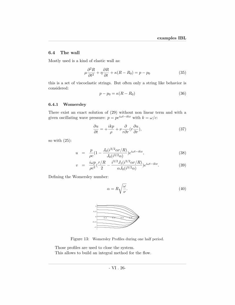
6.4.1 Womersley

There exist an exact solution of (29) without non linear term and with agiven oscillating wave pressure: p = peiωt−ikx with k = ω/c:

∂u

∂t= +

ikp

ρ+ ν

∂

r∂r(r

∂u

∂r), (37)

so with (25):

u =p

ρc(1− J0(i3/2αr/R)

J0(i3/2α))eiωt−ikx, (38)

v =iωp

ρc2(r/R

2− i3/2J1(i3/2αr/R)

αJ0(i3/2α))eiωt−ikx. (39)

Defining the Womersley number:

α = R

√ω

ν. (40)

tuyau souple 9

Ou, si on préfère, sur une demi période on a reporté toutes les vitesses:

0.2 0.4 0.6 0.8 1

-1

-0.5

0

0.5

1

3-5 fermeture du système intégral.

Comme en aérodynamique, le système d'équations globales:

!

!"

!

!

" !

! "

!

!

h

tU

h

x

h U

x h

q

x+ +

+#

+=2 0

2 0

2

1

2

1 2

10

/,

!

!"

!

!

!

!$

%

!

!& %

!

!&& &

q

t xq U

xq u u+ # = # +

'

()

*

+,

= =

2 2 0 2

1

2

2

2

0

22 2

( ) ,

!

!"

!

! -$%

!

!&&

U

tU

xU

dp

dx Ru0

2 0 0 2 2

2

2

0

22

+ = # +'

()

*

+,

=

.

n'est pas un système fermé. Pour résoudre cette difficulté, une méthode originale, due àPohlhausen (Schlichting (1987)) consiste à se donner un champ des vitesses approximatif. Cedernier respecte les conditions aux limites d'adhérence et approche au mieux les profilsexpérimentaux.Nous gardons ici l'esprit de la méthode mais nous l'adaptons au cas instationnaire. Dans larecherche d'un profil pertinent, nous sommes guidés par l'étude du problème linéarisé pourlequel nous disposons de la solution analytique de Womersley écrite en formulation complexe(Womersley (1955)) sous la forme ad hoc:

U F x t iG x t j ijWomersley r i= + +( ( , ) ( , ))( ( ) ( ))%& %&

où on a séparé la dépendance en x et t de la dépendance dans le rayon réduit !=r/R.

( ( , ) ( , )) (( )

)/

( )F x t iG x tkp

J iei t kx

+ = # #

. %.1

1

0

3 2

( ( ) ( ))

(( )

( ))

(( )

)

/

/

/

j ij

J i

J i

J i

r i%& %&

%&

%

%

+ =

#

#

1

11

0

3 2

0

3 2

0

3 2

,

cette dernière fonction est ainsi posée de manière à être égale à 1 au centre.

Dans la suite, on approxime le champ des vitesses en conservant la même dépendance en

variable radiale !. Ce qui, d'une certaine manière, suppose que c'est le mode fondamental quiimpose la structure radiale de l'écoulement. Belardinelli & Cavalcanti 1992 proposent unedécomposition sur des profils de vitesse qui ne sont pas physiques sauf dans le cas Poiseuille.Zagzoule & al 86 utilisent des profils fondés principalement sur Poiseuille.

On pose donc ([z]* est le complexe conjugué de z):

Figure 13: Womersley Profiles during one half period.

Those profiles are used to close the system.This allows to build an integral method for the flow.

- VI . 26-

examples IBL

6.4.2 Closure

As in aerodynamics, the previous system of equations is not closed: we havelost details of the velocity profile in the integration process. Therefore, wehave to imagine a velocity profile and deduce from it relations linking Γ, τand τ0 and q, U0 et R. These relations are found from the radial dependenceof u. Pohlhausen’s idea, explained in Schlichting (1987) [2] or Le Balleur(1982) [1], consists in postulating an ad hoc velocity distribution in η whichfits the boundary conditions and ”looks like” observed profiles. Here themost simple idea is to use the profiles from the analytical linearized solutiongiven by Womersley (1955) [43] for the case with no transverse pressurevariation that we have already seen. This solution in complex form (i2 = −1)is rewritten as:

UWomersley = (FW (x, t) + iGW (x, t))(jr(αη) + iji(αη)), (41)

where FW , GW , ji and jr are real functions defined as follows:

(FW (x, t)+iGW (x, t)) =kp

c(1− 1

J0(i3/2α))ei2π(t−x/c), (jr+iji) =

1− J0(i3/2αη)

J0(i3/2α)

1− 1J0(i3/2α)

.

Thus, we will assume that the velocity distribution in the following has thesame dependence on η. It means that we suppose that the fundamentalmode imposes the radial structure of the flow. The real velocity is:

u = 1/2 ((F + iG)(jr + iji) + cc) = (Fjr −Gji), (42)

where F (x, t) and G(x, t) are now real unknown functions that we want tofind and cc is the conjugate complex. We immediately see that U0(x, t) =F (x, t) (because jr(0) = 1 and ji(0) = 0) and that if we compute q with(42) we obtain G(x, t) as:

G(x, t) =q/R2 − U0 + U02

∫ 10 jrηdη

2∫ 10 jiηdη

. (43)

The two functions F and G are only functions of (U0, R, q) and we keep theWomersley radial dependence.

6.4.3 The coefficients of closure

The velocity at any radius η (42) and (43) may be written with the value ofthe velocity at the centre U0 ,the radius R, and the loss of flux q. Next, by

- VI . 27-

examples IBL

integration, we obtain Γ as a function of (U0, R, q) and, by derivation, weobtain τ and τ0 as functions of (U0, R, q):

Γ = γqqq2

R2+ γquqU0 + γuuR2U2

0 , τ = τqq

R2+ τuU0 τ0 = τ0q

q

R2+ τ0uU0.

(44)This closes the problem. The coefficients ((γqq, γqu, γuu), (τq, τu), (τ0q, τ0u))are only functions of α. They involve combinations of integrals and deriva-tives of the Bessel function. For example we have (if

∫f is a shorthand for∫ 1

0 f(η)dη and ∂ηfη=0 an other for ∂f∂η (0)):

γuu = 1−∫

j2i /(

∫ji)

2 − (2∫

jrji)/∫

ji −∫

j2r +

+(2∫

j2i

∫jr)/(

∫ji)

2 + (2∫

jijr

∫jr)/

∫ji −

−(∫

j2i (

∫jr)

2)/(∫

ji),

τ0u = ∂2ηjrη=0 + ∂2

ηjiη=0/

∫ji − (∂2

ηjiη=0

∫jr)/

∫ji.

These coefficients are nearly constant for α < 5. For α small we obtain fromthe preceding computations:

((−65

,115

,−215

), (24,−12), (−12, 4)), (45)

so, we recover the values for the Poiseuille profile at small frequency. Thefact that those coefficients are nearly constant makes the model robust. Forα →∞ (in practice, α > 12 is enough) we find from asymptotic behaviour ofBessel functions and from the preceding computations the asymptotic formof the coefficients:

((−α

4√

2, 2,−

√2

2α), (α2/2,−α

√2), (0, 0)).

One can easily show that this is coherent with Wormesley’s solution in thelimit of large α. We note that for α →∞ and ε2 = 0, the wave solution forq is

q =√

2απ

(1− i)e2iπ(t−x/x), c =

√k

2(1−

√2

α(1− i) + O(α−2).

Now equations (??), (32), (33) and (34 ) with the closure (44) define a setof four monodimensional equations linking the pressure p, the velocity alongthe axis U0, the loss of flux q and the variation of the radius h.

- VI . 28-

examples IBL

6.4.4 Remarks

1- The main difference from other integral methods ([40] , [41], [42], [46],[45], or [44] ...) in our approach is the introduction of an auxillary partialdifferential relation (33) obtained from an aeronautical analogy. Instead ofq, Γ and U0 authors mainly use Q, Q2 and U0:

Q =∫ R

02πurdr Q/π = U0R

2 − q

Q2 =∫ R

02πru2dr Q2/π = U2

0 R2 − Γ

If we substract (32) from (33) we obtain the classical system of two equa-tions:

2πR∂R

∂t+ ε2

∂

∂x(Q) = 0,

∂Q

∂t+ ε2

∂

∂x(Q2) = −πR2 ∂p

∂x+ π

2π

α2(∂u

∂η)|η=1

Often, the relation for Q2 is written as Q2 = Q2

πR2 (in this case the radial vari-

ation of the profile is neglected: flat profile) or Q2 = 4Q2

3πR2 (parabolic profile:see equation (45)). Note, that we have instead a third differential equationto link Q1 and Q2. The effect of the skin friction (τ1 = 2π

α2 (∂u∂η )|η=1) is often

estimated by τ1= − 8πα2

QπR3 , true for a Poiseuille flow only ((45) again). It

may be replaced by an unsteady relation (deduced from unsteady Poiseuilleflow) such as:

Tτ∂τ1

∂t+ τ1 = − 8

α2(Q + TQ

∂Q

∂t+ ...)

See Yama et al (1995) [44] for the derivations and values of coefficients Tτ

and TQ. We do not claim that our description is better, but for a sinusoidalinput we find again (at any frequency) the Womersley linear solution. Ourprofiles are realistic in the sense that they present overshoots in the coreand back flow near the wall. This is not the case when the closure is simplyτ1= − 8π

α2Q

πR3 or in the case of very peculiar profiles chosen by Belardinelli &Cavalcanti (1992) [36].

2- We noted that the coefficients vary little with α, this shows that ourmodel is very robust: it is easy to see that equations (32) and (33) areinvariant under the rescaling t → t/Ω, /

√Ω, and c → c, if τ is taken con-

stant (independant of α). This explains why methods based on Poiseuillecoefficients are robust too.

- VI . 29-

examples IBL

6.5 Interactive problem

The interactive problem is mainly solved in an 1D description ([40], [45]). Aspeople solved linearised systems at first, it was clear that those equationsreduce to wave equations and need two boundary conditions one at theentrance, the other at the output. Some solutions of the full interactingproblem have been done by [38] and [37]

7 Conclusion on Interactive problems

No definite conclusion will be given, we insist on the fact that some thinlayer flows must be solved with the good set of boundary conditions. Thesupersonic paradox of the ”free interaction” is in fact present in a lot offlows (hypersonic, mixed convection, artery, supercritical...).

References

[1] Le Balleur J.C. (1982): ”Viscid- inviscid coupling calculations for 2 and3D flows”, VKI lecture series 1982-02.

[2] Schlichting H. (1987): ”Boundary layer theory”, Mc Graw Hill.

[3] F.T. Smith (1979): ”On the non parallel flow stability of the blasiusboundary layer”, Proc. Roy. Soc. Lond., A366, pp. 91- 109.

[4] F. T. Smith (1982): ”On the high Reynolds Number Theory of LaminarFlows”, IMA Journal of Applied Mathematics, vol 28, pp. 207-281.

Hypersonic

[5] S.N. Brown, K. Stewartson & P.G. Williams (1975): ”Hypersonic selfinduced separation”, The Phys. of Fluids, vol 18, No 6, June.

[6] S. N. Brow H. & K. Cheng Lee (1990): ”Inviscid viscous interactionon triple deck scales in a hypersonic flow with strong wall cooling”, J.Fluid Mech., vol 220, pp. 309- 307.

[7] S.N. Brown & K. Stewartson P.G. (1975): ”A non uniqueness of thehypersonic boundary layer”, Q.J. appl Math, vol XXVIII, Pt 1 pp. 75-90

[8] Chernyi (1961): ”Introduction to hypersonic flow” , Academic Press

- VI . 30-

examples IBL

[9] Guiraud, J. P., Vallee, D., Zolver, R. 1965. In Basic Developments inFluid Dynamics. ed. M, Holt, 127-247, New York : Academic. 447 pp.

[10] Hayes & Probstein (1959):”Hypersonic flow theory” Academic Press .

[11] P.-Y. Lagree (1992): ”Structures interactives Fluide Parfait/ Couchelimite en hypersonique, Variations autour du theme de la triple couche”,These de l’Universite Paris VI,

[12] P.-Y. Lagree (1991): ”Influence de la couche d’entropie sur la longueurde separation en aerodynamique hypersonique, dans le cadre de la triplecouche II”, C.R. Acad Sci Paris, t 313, Serie II, p. 999-1004, 1991.

[13] P.-Y. Lagree (1990): ”Influence de la couche d’entropie sur l’echellede la region separee en aerodynamique hypersonique”, C.R. Acad SciParis, t 311, Serie II, p. 1129- 1134, 1990.

[14] V. Ya Neiland (1969): ”Theory of laminar boundary layer separationin supersonic flow ”, Mekh. Zhid. Gaz., Vol. 4, pp. 53-57.

[15] V. Ya Neiland (1970): ”Propagation of perturbation upstream withinteraction between a hypersonic flow and a boundary layer”, Mekh.Zhid. Gaz., Vol. 4, pp. 40-49.

[16] V. Ya Neiland (1986): ” Some features of the transcritical bound-ary layer interaction and separation”, IUTAM London SN Brown edi.Springer

[17] A. I. Ruban & S. N. Timoshin (1986): ”Propagation of perturbationsin the boundary layer on the walls of a flat chanel”, Fluid Dynamics,No 2, pp. 74-79.

[18] L.I. Sedov: 1959 ”Similarity and Dimensional Methods in Mechanics.”Infosearch Ltd., London., 1959,”Similitude et dimensions en mecanique”, editions Mir, 1977.

[19] Stewartson K. (1964) ”the Theory of Laminar Boundary Layers in Com-pressible Fluids”, Oxford University Press, London (1964).

[20] K. Stewartson & P.G. Williams (1969): ”Self - induced separation”,ProcRoy Soc, A 312, pp 181-206.

[21] Milton Van Dyke (1982) ”An Album of Fluid Motion.” Stanford TheParabolic Press.

- VI . 31-

examples IBL

[22] M. J. Werle, D. L. Dwoyer a W. L. Hankey (1973) ”Initial conditionsfor the hypersonic-shock/ boundary- layer interaction problem”, AIAAJ., vol 11, no 4, pp525- 530.

[23] Thermal Flows

[24] F. J. Higuera (1997): ”Opposing mixed convection flow in a wall jetover a horizontal plate” J. Fluid Mech., vol 342, pp. 355-375.

[25] P.G. Daniels (1992): ”A singularity in thermal boundary- layer flow ona horizontal surface”, J. Fluid Mech., vol 242, pp. 419- 440.

[26] P.G. Daniels & R.J. Gargaro (1993): ” Buoyancy effects in stablystratified horizontal boundary- layer flow”, J. Fluid Mech., Vol. 250,pp. 233- 251.

[27] M. El Hafi (1994): ”Analyse asymptotique et raccordements, etuded’une couche limite de convection naturelle”, these de l’Universite deToulouse.

[28] Exner, A ; Kluwick, A (2001). ”On thermally induced separation oflaminar free-convection flows” Physics of Fluids, Volume 13, Issue 6,pp. 1691-1703 (2001).

[29] P.-Y. Lagree (1994): ”Convection thermique mixte a faible nombre deRichardson dans le cadre de la triple couche”, C. R. Acad. Sci. Paris,t. 318, Serie II, pp. 1167- 1173.

[30] P.-Y. Lagree (1995): ”Upstream influence in mixed convection at smallRichardson Number on triple, double and single deck scales”, symp.:Asymptotic Modelling in Fluid Mechanics, Bois, Deriat, Gatignol &Rigolot (Eds.), Lecture Notes in Physics, Springer, pp. 229-238.

[31] P.-Y. Lagree (2001): ”Removing the marching breakdown of the bound-ary layer equations for mixed convection above a horizontal plate”,International Journal of Heat and Mass Transfer, Vol 44/17, pp. 3359-3372.

[32] W. Schneider & M.G. Wasel (1985): ”Breakdown of the boundary layerapproximation for mixed convection above an horizontal plate”, Int. J.Heat Mass Transfert , Vol. 28, No 12, pp. 2307-2313.

[33] H. Steinruck (1994): ”Mixed convection over a cooled horizontal plate:non-uniqueness and numerical instabilities of the boundary layer equa-tions”, J. Fluid Mech., vol 278, pp. 251-265

- VI . 32-

examples IBL

[34] H. Steinruck (1995): ”Mixed convection over a horizontal plate: selfsimilar and connecting boundary- layer flows”, Fluid Dynamic Res, 15,pp 113- 127.

[35] Blood Flows

[36] Belardinelli E. & Cavalcanti S. (1992): ”theorical analysis of pressurepulse propagation in arterial vessels”, J. Biomechanics vol 25 pp. 1337-1349.

[37] Canic, S.; Hartley, C.; Rosenstrauch, D.; Tambaca, J. Guidoboni, G.;Mikelic, A. (2006) ”Blood Flow in Compliant Arteries: An EffectiveViscoelastic Reduced Model, Numerics, and Experimental Validation”Annals of Biomedical Engineering, Vol. 34, No. 4, April 2006 (2006)pp. 575–592

[38] P.-Y. Lagree (2000): ”An inverse technique to deduce the elasticity ofa large artery ”, European Physical Journal, Applied Physics 9, pp.153-163

[39] Ling S.C. & Atabek H.B. (1972): ”a non linear analysis of pulsatile flowin arteries” J.F.M. vol 55 p 3 pp.

[40] Olufsen MS, Peskin CS, Kim WY, Pedersen EM, Nadim A, Larsen J.(2000): ”Numerical simulation and experimental validation of bloodflow in arteries with structured-tree outflow conditions.” Ann BiomedEng. 2000 Nov-Dec;28(11):1281-99.

[41] Pedley T. J. (1980): ”The Fluid Mechanics of Large Blood Vessel”,Cambridge University press.

[42] Pythoud F., Stergiopulos N. & Meister J.-J. (1996): ”Separation ofarterial pressure waves into their forward and backward running com-ponents”, J. Biom. Eng., august, vol 118, pp. 295- 301.

[43] Womersley J. R. (1955): ”Oscillatory Motion of a Viscous Liquid in aThin- Walled Elastic Tube”, Philosophical Magazine, volume 46, pages199-221.

[44] Yama J.R., Mederic P. & Zagzoule M. (1995): ”Etude comparativedes differentes approximations de la contrainte de cisaillement a laparoi”Archives of Physiology and Biochemestry, vol 103, N 3, Jullyp C164.

- VI . 33-

examples IBL

[45] Zagzoule M. & Marc- Vergnes J.-P (1986) ”a global mathematical modelof the cerebral circulation in man”, J. Biomechanics Vol 19, No 12, pp.1015-1022.

[46] Zagzoule M. J. Khalid- Naciri & J. Mauss (1991): ”Unsteady wall shearstress in a distensible tube”, J. Biomechanics Vol 24, No 6, pp. 435-439.

[47] Saint Venant

[48] R.I. Bowles & F.T. Smith (1992): ”The standing hydraulic jump: the-ory, computations and comparisons with experiments”, J. Fluid Mech.,vol 242, pp. 145-168.

[49] J. Gajjar & F.T. Smith (1983): ”On hypersonic self induced separation,hydraulic jumps and boundary layer with algebraic growth”, Mathe-matika, 30, pp. 77-93.

[50] F. J. Higuera (1994): ”The hydraulic jump in a viscous laminar flow”J. Fluid Mech., vol 274, pp. 62-92.

[51] F. J. Higuera (1997): ”The circular hydraulic jump ” Phys. Fluids 9(5), May 1997 pp. 1476-1479.

The web page of this text is:http://www.lmm.jussieu.fr/∼lagree/COURS/CISM/

The last version of this file is on:http://www.lmm.jussieu.fr/∼lagree/COURS/CISM/ex−CISM.pdf

- VI . 34-