solving sets of equations - caig labcaig.cs.nctu.edu.tw/course/nm07s/slides/chap2_2.pdf · solving...
TRANSCRIPT

Solving Sets of Equations
150 B.C.E., 九章算術 Carl Friedrich Gauss, 1777-1855
Numerical Methods © Wen-Chieh Lin 2
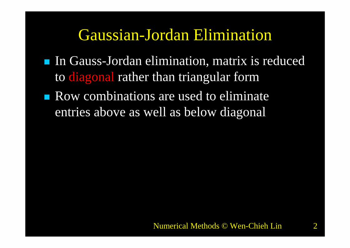
Gaussian-Jordan Elimination In Gauss-Jordan elimination, matrix is reduced
to diagonal rather than triangular formRow combinations are used to eliminate
entries above as well as below diagonal

Numerical Methods © Wen-Chieh Lin 3
Gaussian-Jordan Elimination (cont.)
Elimination matrix used for given columnvector a is of form
niaam
a
a
aa
a
a
m
m
m
m
kii
k
n
k
k
k
n
k
k
,,1,where
0
0
0
0
1000
0100001000010
0001
1
1
1
1
1
1
aMk

Numerical Methods © Wen-Chieh Lin 4
Gaussian-Jordan Elimination (cont.)Gauss-Jordan elimination requires about n3/2
multiplications and similar number ofadditions, 50% more expensive than LUfactorization
During elimination phase, same row operationsare also applied to right-hand-side vector(vectors) of system of linear equations
Once matrix is in diagonal form, componentsof solution are computed by dividing eachentry of transformed right-hand side bycorresponding diagonal entry of matrix

Numerical Methods © Wen-Chieh Lin 5
Using LU for multiple right-hand sides
If LU factorization of a matrix A is given, wecan solve Ax = b for different b vectors asfollows:
Ax = b LUx = b Solve Ly = b using forward substitution Then solve Ux = y using backward substitution
Numerical Methods © Wen-Chieh Lin 6
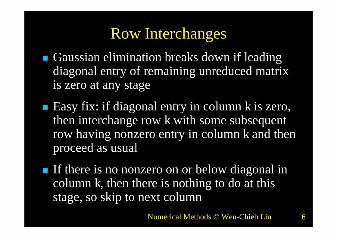
Row InterchangesGaussian elimination breaks down if leading
diagonal entry of remaining unreduced matrixis zero at any stage
Easy fix: if diagonal entry in column k is zero,then interchange row k with some subsequentrow having nonzero entry in column k and thenproceed as usual
If there is no nonzero on or below diagonal incolumn k, then there is nothing to do at thisstage, so skip to next column

Numerical Methods © Wen-Chieh Lin 7
Row Interchanges (cont.) Zero on diagonal causes resulting upper
triangular matrix to be singular, but LUfactorization can still be completed
Subsequent back-substitution will fail,however, as it should for singular matrix

Numerical Methods © Wen-Chieh Lin 8
Partial Pivoting
In principle, any nonzero value will do as pivot,but in practice pivot should be chosen tominimize error propagation
To avoid amplifying previous rounding errorswhen multiplying remaining portion of matrixby elementary elimination matrix, multipliersshould not exceed 1 in magnitude
This can be accomplished by choosing entry oflargest magnitude on or below diagonal aspivot at each stage
Numerical Methods © Wen-Chieh Lin 9
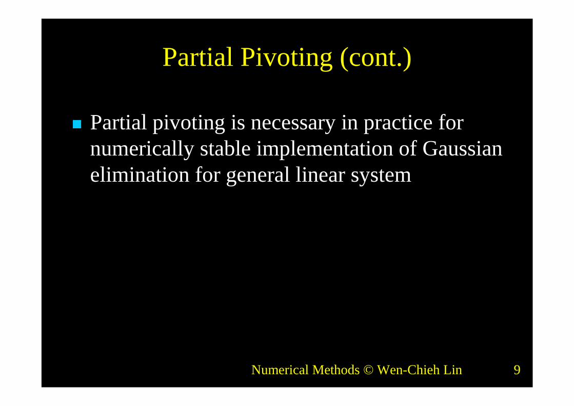
Partial Pivoting (cont.)
Partial pivoting is necessary in practice fornumerically stable implementation of Gaussianelimination for general linear system

Numerical Methods © Wen-Chieh Lin 10
LU Factorization with Partial Pivoting
With partial pivoting, each Mk is preceded bypermutation Pk to interchange rows to bringentry of largest magnitude into diagonal pivotposition
Still obtain MA = U, with U upper triangular,but now
M = Mn-1Pn-1···M1P1
L=M-1 is not a triangular due to permutations
nTn
TTnn LPLPLPPMPMPMML 2211
111222
1 )(
Numerical Methods © Wen-Chieh Lin 11
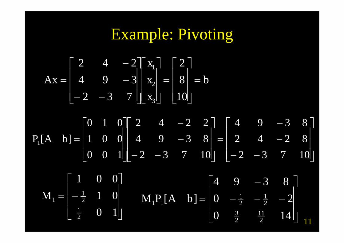
Example: Pivoting
bAx
1082
732394242
3
2
1
xxx
1073282428394
1073283942242
100001010
][1 bAP
1001001
21
21
1M
14020
8394][
211
23
21
21
11 bAPM

Numerical Methods © Wen-Chieh Lin 12
Example: Pivoting (cont.)
14020
8394
010100001
][
211
23
21
21
112 bAPMP
38
34
211
23
001408394
201408394
10010001
][
21
21
211
23
31
1122 bAPMPM

Numerical Methods © Wen-Chieh Lin 13
Example: Pivoting (cont.)
010011
)(
21
31
21
22111
11221 LPLPPMPMML TT
38
34
211
23
001408394
U is still upper triangular butL is not lower triangular due to permutations

Numerical Methods © Wen-Chieh Lin 14
Complete PivotingComplete pivoting is more exhaustive strategy
in which largest entry in entire remainingunreduced submatrix is permuted into diagonalpivot position
Requires interchanging columns as well asrows leading to factorization
PAQ = LUwith L unit lower triangular, U uppertriangular, and P, Q permutations

Numerical Methods © Wen-Chieh Lin 15
Complete Pivoting (cont.)
Numerical stability of complete pivoting istheoretically superior, but pivot search is moreexpensive than for partial pivoting
Numerical stability of partial pivoting is morethan adequate in practice, so it is almostalways used in solving linear system byGaussian elimination
Numerical Methods © Wen-Chieh Lin 16
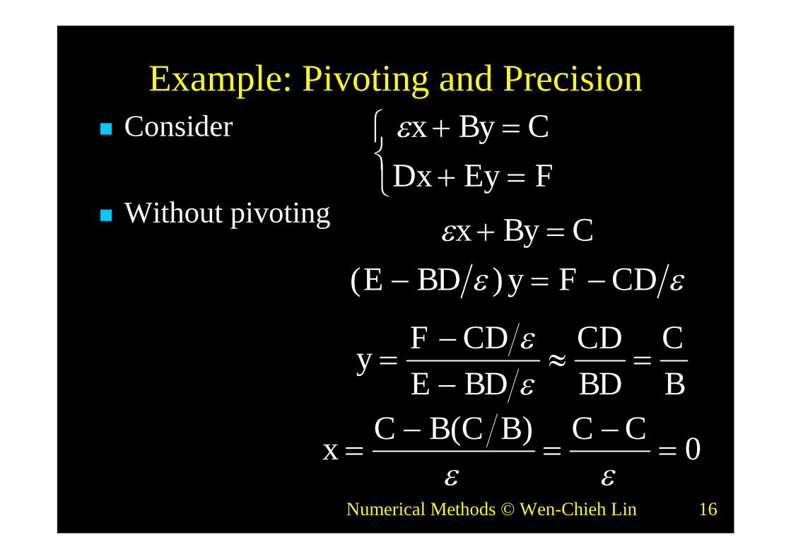
Example: Pivoting and PrecisionConsider
Without pivoting
FEyDxCByx
CDFyBDECByx
)(
BC
BDCD
BDECDF
y
0)(
CCBCBCx
Numerical Methods © Wen-Chieh Lin 17
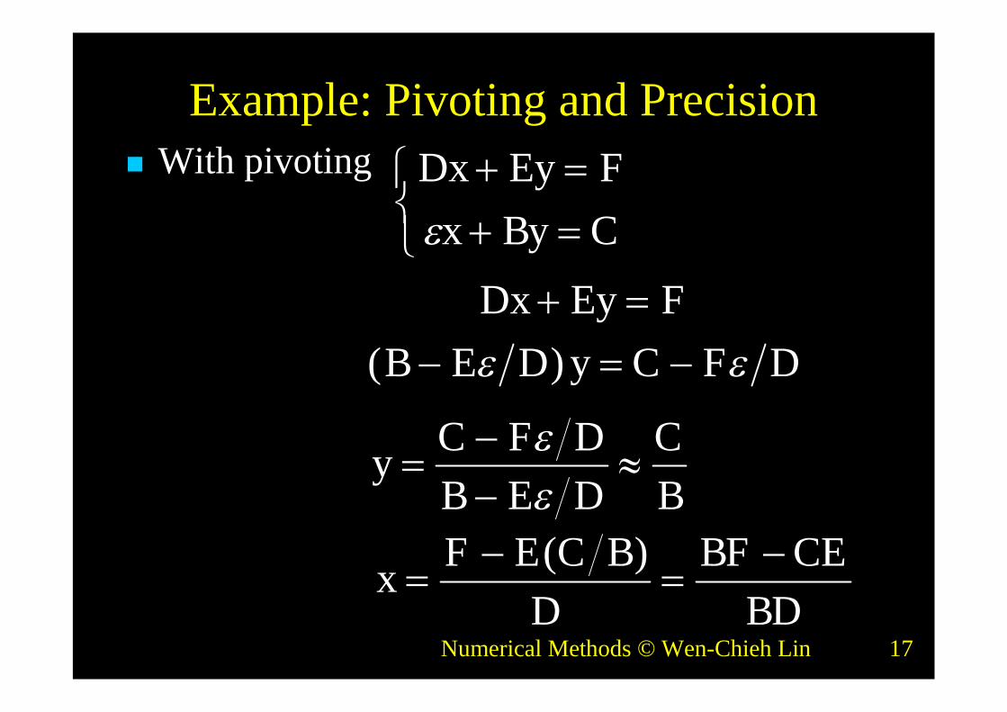
Example: Pivoting and PrecisionWith pivoting
CByxFEyDx
DFCyDEBFEyDx
)(
BC
DEBDFC
y
BDCEBF
DBCEF
x
)(
Numerical Methods © Wen-Chieh Lin 18
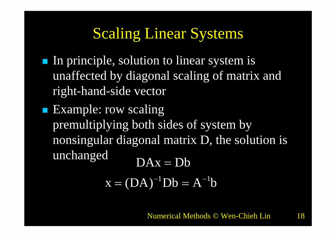
Scaling Linear Systems
In principle, solution to linear system isunaffected by diagonal scaling of matrix andright-hand-side vector
Example: row scalingpremultiplying both sides of system bynonsingular diagonal matrix D, the solution isunchanged DbDAx
bADbDAx 11)(

Numerical Methods © Wen-Chieh Lin 19
Scaling Linear Systems (cont.)
In practice, scaling affects both conditioning ofmatrix and selection of pivots in Gaussianelimination, which in turn affect numericalaccuracy in finite-precision arithmetic
It is usually best if all entries of matrix haveabout same size

Numerical Methods © Wen-Chieh Lin 20
Scaling Linear Systems (cont.)
Sometimes it may be obvious how toaccomplish this by choice of measurementunits for variables, but there is no foolproofmethod for doing so in general
Scaling can introduce error if not donecarefully!

Numerical Methods © Wen-Chieh Lin 21
Example: Scale Partial Pivoting Given
the exact solution is x = [1, 1, 1]T
If only 3 digits of precision is used
we obtain a erroneous solutionx = [0.939, 1.09, 1.00]T
2102105
,121
1003110023
bA
6.824.820013513367.3010510023
Numerical Methods © Wen-Chieh Lin 22
Example: Scale Partial Pivoting (cont.) Premultiplying by a scaling matrix
2/1000100/1000100/1
S
00.150.000.150.035.100.103.001.005.100.102.003.0
][ bAS
2102105
,121
1003110023
bA
Pivoting is required at the first column!

Numerical Methods © Wen-Chieh Lin 23
Example: Scale Partial Pivoting (cont.) In algorithm implementation, we don’t scale
equations explicitly Instead, we store the scale vector and row
interchange information and only use them forpivot selection
99103401049950
2121
21211021003110510023
1001002s
182182001049950
2121
partial pivoting no pivoting is required

Numerical Methods © Wen-Chieh Lin 24
Complexity of Solving Linear System
LU factorization requires about n3/3 floating-point multiplications and similar number ofadditions
Forward and backward substitution for singleright-hand side vector together require about n2
multiplications and similar number ofadditions
Numerical Methods © Wen-Chieh Lin 25
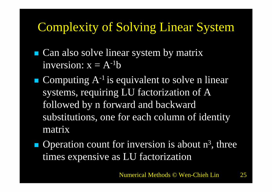
Complexity of Solving Linear System
Can also solve linear system by matrixinversion: x = A-1b
Computing A-1 is equivalent to solve n linearsystems, requiring LU factorization of Afollowed by n forward and backwardsubstitutions, one for each column of identitymatrix
Operation count for inversion is about n3, threetimes expensive as LU factorization

Numerical Methods © Wen-Chieh Lin 26
Inversion vs. Factorization
x=A-1bNeeds to solve Ax = ILU factorization n forward and
backward substitutionsMultiplication of
matrix and vector
LUx = bLU factorizationOne forward and
backward substitution

Numerical Methods © Wen-Chieh Lin 27
Inversion vs. Factorization (cont.) Inversion gives less accuracy answer; e.g.,
solving 3x = 18 by division gives x = 18/3 = 6,but inversion gives x = 3-1 × 18 = 0.333 × 18 =5.99 (using 3-digit arithmetic)
Numerical Methods © Wen-Chieh Lin 28
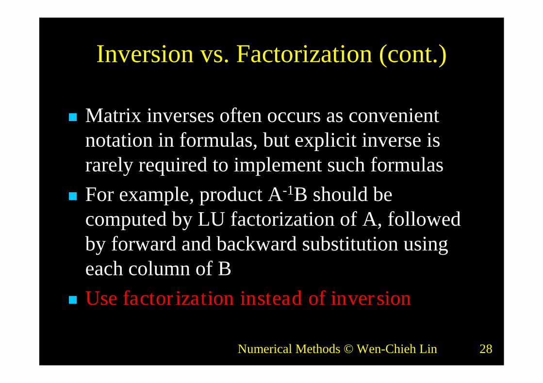
Inversion vs. Factorization (cont.)
Matrix inverses often occurs as convenientnotation in formulas, but explicit inverse israrely required to implement such formulas
For example, product A-1B should becomputed by LU factorization of A, followedby forward and backward substitution usingeach column of B
Use factorization instead of inversion

Numerical Methods © Wen-Chieh Lin 29
Ill-Conditioned Systems Recall that“A system is ill-conditioned if the solution isvery sensitive to changes in the input”
Example: a near-singular coefficient matrix
00.200.2
01.199.099.001.1
yx
00.100.1
yx
98.102.2
b
000.2
yx
02.298.1
b
00.20
yx
We cannot test the accuracy of the computed solution merelyby substituting the solution into equation to see whether theright-hand sides are reproduced
Numerical Methods © Wen-Chieh Lin 30
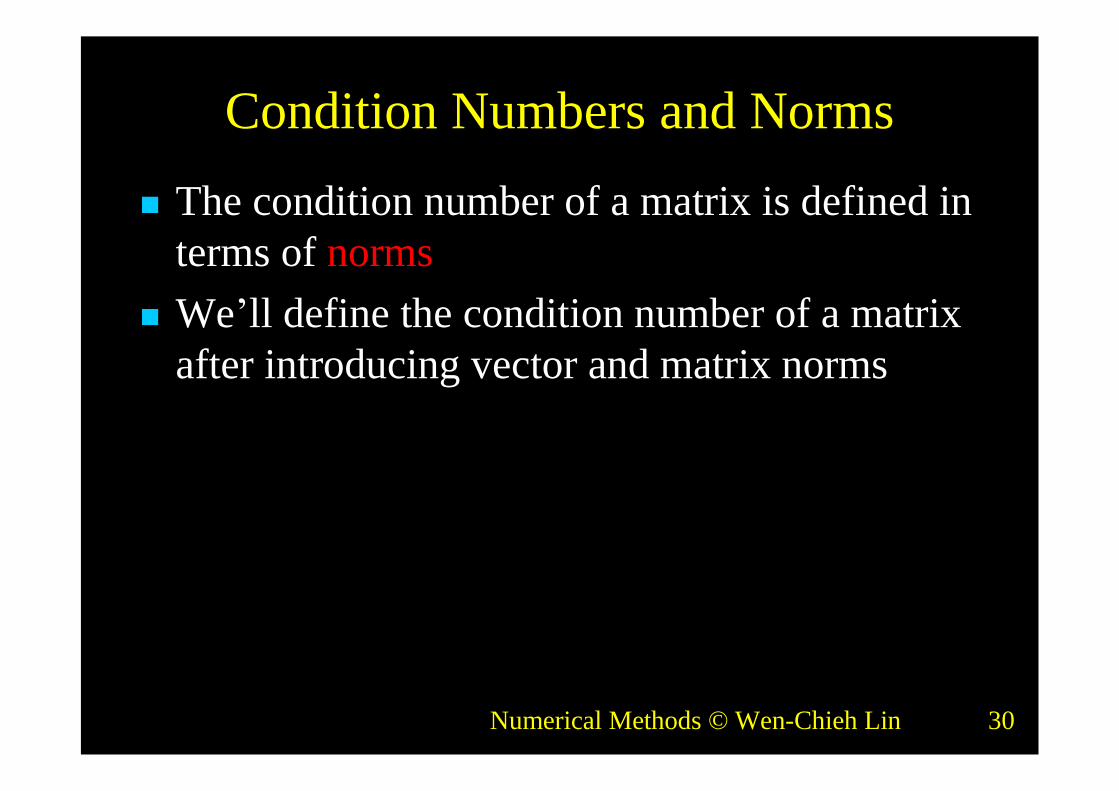
Condition Numbers and Norms
The condition number of a matrix is defined interms of norms
We’ll define the condition number of a matrixafter introducing vector and matrix norms
Numerical Methods © Wen-Chieh Lin 31
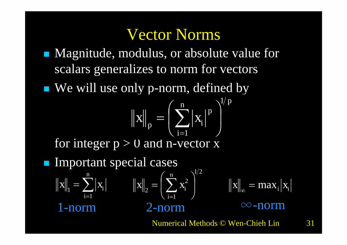
Magnitude, modulus, or absolute value forscalars generalizes to norm for vectors
We will use only p-norm, defined by
for integer p > 0 and n-vector x Important special cases
1
1
pn
i
pip
xx
Vector Norms
21
1
22
n
iixx
n
iixx
11 ii xx max
1-norm ∞-norm2-norm

Numerical Methods © Wen-Chieh Lin 32
Properties of Vector Norms For any vector norm
The definition of a vector norm needs tosatisfies the above properties
)inequalityr(triangula
scalaranyfor
0ifonlyandif0and0
yxyx
xx
xxx
kkk
Numerical Methods © Wen-Chieh Lin 33
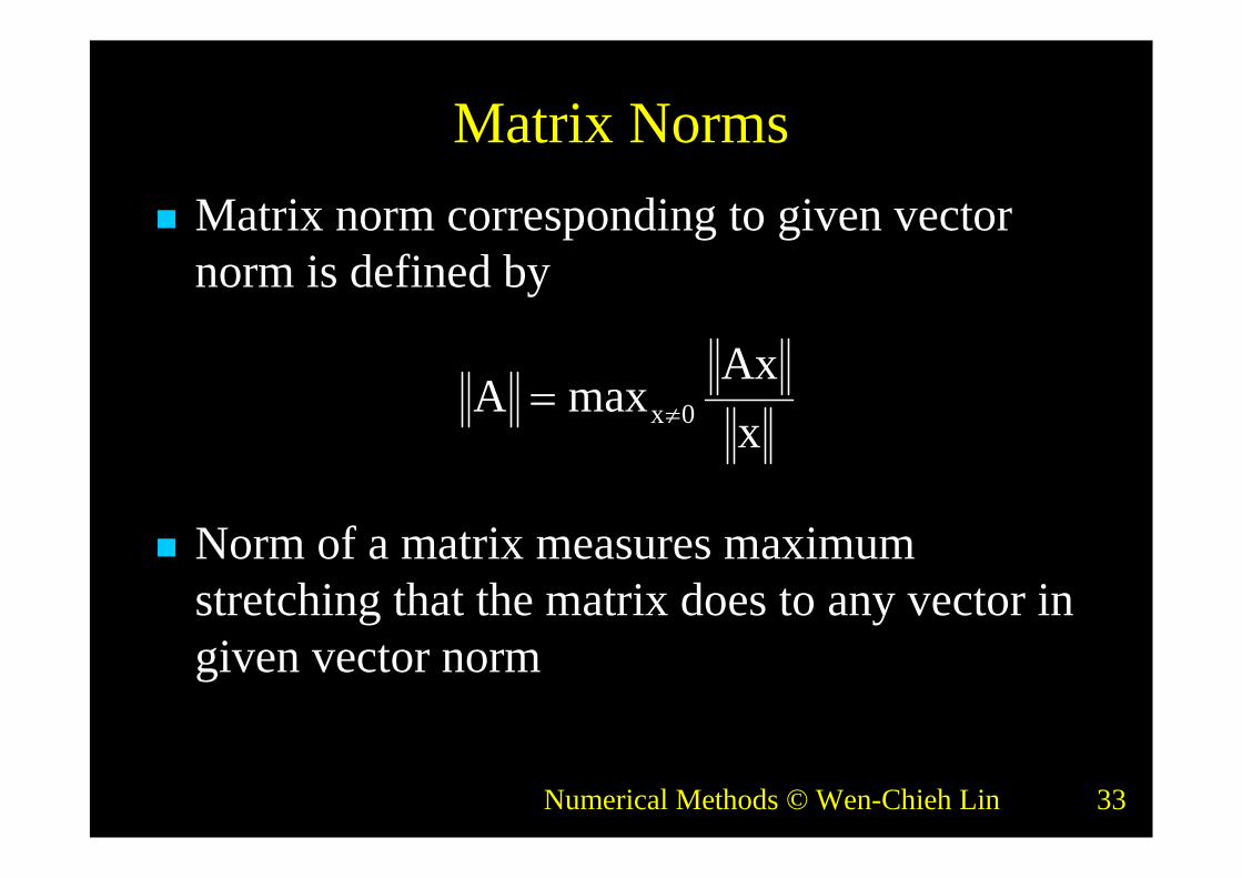
Matrix NormsMatrix norm corresponding to given vector
norm is defined by
Norm of a matrix measures maximumstretching that the matrix does to any vector ingiven vector norm
xAx
A x 0max
Numerical Methods © Wen-Chieh Lin 34
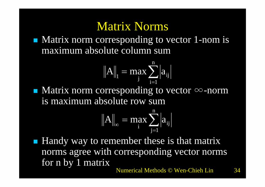
Matrix NormsMatrix norm corresponding to vector 1-nom is
maximum absolute column sum
Matrix norm corresponding to vector ∞-normis maximum absolute row sum
Handy way to remember these is that matrixnorms agree with corresponding vector normsfor n by 1 matrix
n
iijj
a1
1maxA
n
jiji
a1
maxA

Numerical Methods © Wen-Chieh Lin 35
Properties of Matrix Norms
Matrix norms we have defined satisfies
Above are actually the required propertieswhen a matrix norm is defined!
BAAB
BABA
kAkkA
AAA
scalaranyfor
0ifonlyandif0and0

Numerical Methods © Wen-Chieh Lin 36
Condition Number Condition number of square nonsingular matrix A
is defined by
By convention, cond(A) = ∞ if A is singular Large cond(A) means A is singular Since
condition number measures ratio of maximumstretching to maximum shrinking does to anynonzero vectors
1)(cond AAA
x
xA
xAx
AAxx
1
00
1 maxmax
Numerical Methods © Wen-Chieh Lin 37
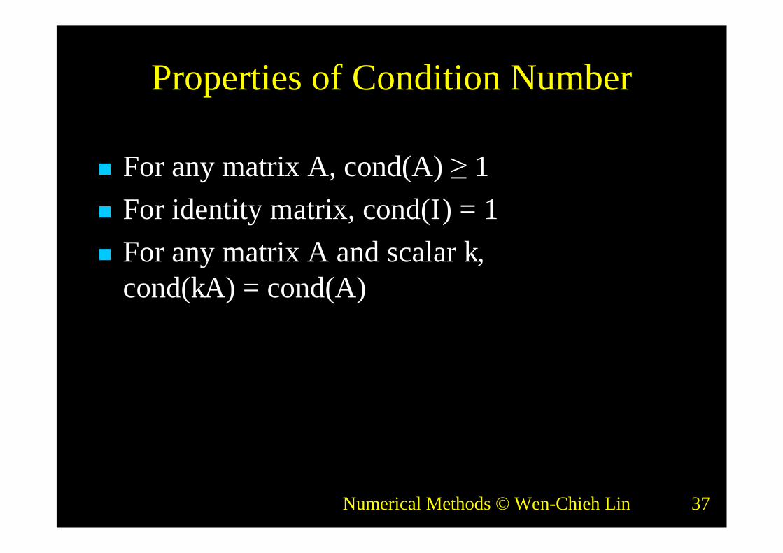
Properties of Condition Number
For any matrix A, cond(A) ≥1 For identity matrix, cond(I) = 1 For any matrix A and scalar k,
cond(kA) = cond(A)

Numerical Methods © Wen-Chieh Lin 38
Computing Condition Number
Definition of condition number involvesmatrix inverse, so it is nontrivial to compute
Computing condition number from definitionwould require much more work thancomputing solution whose accuracy is to beassessed
In practice, condition number is estimatedinexpensively as byproduct of solution process

Numerical Methods © Wen-Chieh Lin 39
Computing Condition NumberMatrix norm is easily computed as
maximum column sum (or row sum,depending on norm used)
Estimating at low cost is morechallenging
From properties of norms, if Az = y, then
and bound is achieved for optimally chosen y
A
1A
111 Ayz
yAyAz
Numerical Methods © Wen-Chieh Lin 40
1A
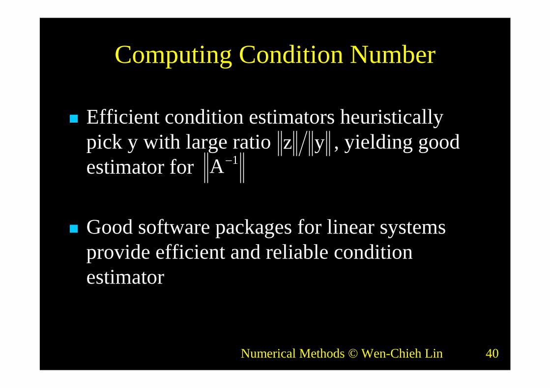
Computing Condition Number
Efficient condition estimators heuristicallypick y with large ratio , yielding goodestimator for
Good software packages for linear systemsprovide efficient and reliable conditionestimator
yz
Numerical Methods © Wen-Chieh Lin 41
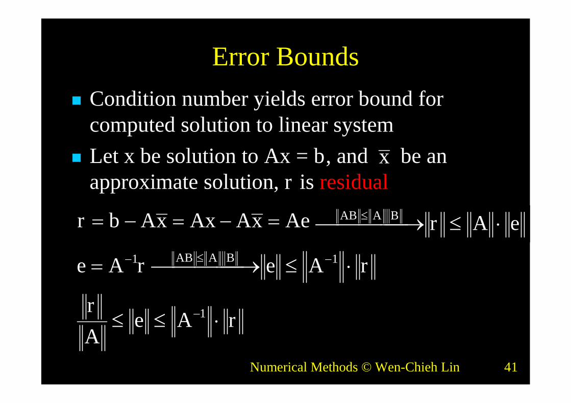
Error BoundsCondition number yields error bound for
computed solution to linear system Let x be solution to Ax = b, and be an
approximate solution, r is residual
AexAAxxAbr
rAerAe BAAB 11
eArBAAB
rAeAr
1
x

Numerical Methods © Wen-Chieh Lin 42
Error Bounds (cont.) Similarly, from b = Ax and x = A-1b we obtain
Combined with previous result
We have
bAxAb
1
rAeAr
1
br
AAxe
br
AA1
1
1
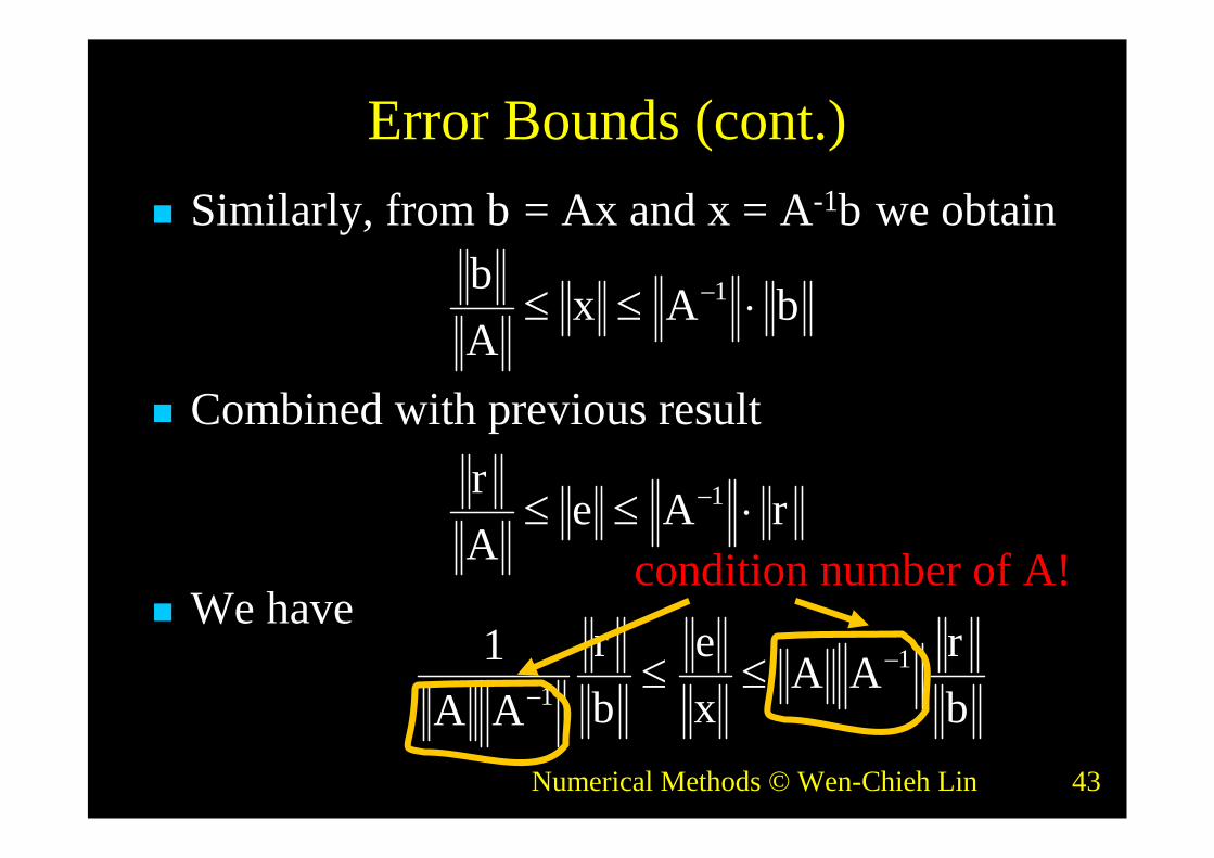
Numerical Methods © Wen-Chieh Lin 43
Error Bounds (cont.) Similarly, from b = Ax and x = A-1b we obtain
Combined with previous result
We have
bAxAb
1
rAeAr
1
br
AAxe
br
AA1
1
1
condition number of A!

Numerical Methods © Wen-Chieh Lin 44
Error Bounds (cont.)
The relative error in the computed solutionvector is bounded by the relative residualdivided/multiplied by the condition number
When the condition number is large, theresidual gives little information about theaccuracy
br
Axe
br
A)(cond
)(cond1
Numerical Methods © Wen-Chieh Lin 45
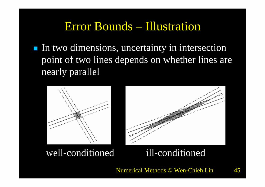
Error Bounds –Illustration
In two dimensions, uncertainty in intersectionpoint of two lines depends on whether lines arenearly parallel
well-conditioned ill-conditioned
Numerical Methods © Wen-Chieh Lin 46
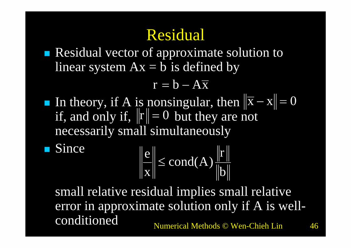
0r
Residual vector of approximate solution tolinear system Ax = b is defined by
In theory, if A is nonsingular, thenif, and only if, but they are notnecessarily small simultaneously
Since
small relative residual implies small relativeerror in approximate solution only if A is well-conditioned
Residual
xAbr 0xx
br
Axe
)cond(

Numerical Methods © Wen-Chieh Lin 47
Iterative Refinement
Given approximate solution x0 to linear systemAx = b, compute residual
Now solve linear system Az0 = r0 and take
as new and “better”approximate solution,since
00 Axbr
0zxx 01
00 )( AzAxzxAAx 001 br)r(b 00

Numerical Methods © Wen-Chieh Lin 48
Iterative Refinement (cont.)
Process can be repeated to refine solutionsuccessively until convergence, potentiallyproducing solution accurate to full machineprecision

Numerical Methods © Wen-Chieh Lin 49
Error in Coefficients of Matrix
Let be the perturbed coefficientmatrix and the solution to the perturbedsystem
Using and
xEAA
bxA bAx
)(11 xAAbAx xxxAA )(1
xAAxAAx 11 )( xEAxxAAAx 11 )(
xEAxx 1

Numerical Methods © Wen-Chieh Lin 50
Error in Coefficients of Matrix (cont.)
Error of the solution relative to the norm of thecomputed solution can be as large as the relativeerror in the coefficients of A multiplied by thecondition number
xEAxx 1
xAE
AAxEAxx 11
AE
Ax
xx)(cond