solving relational mdps with exogenous events and additive

Solving Relational MDPs with Exogenous Events andAdditive Rewards

Saket Joshi1, Roni Khardon2, Prasad Tadepalli3, Aswin Raghavan3, and Alan Fern3

1 Cycorp Inc., Austin, TX, USA2 Tufts University, Tufts University, Medford, MA, USA

3 Oregon State University, Corvallis, OR, USA

Abstract. We formalize a simple but natural subclass of service domains for re-lational planning problems with object-centered, independent exogenous eventsand additive rewards capturing, for example, problems in inventory control. Fo-cusing on this subclass, we present a new symbolic planning algorithm which isthe first algorithm that has explicit performance guarantees for relational MDPswith exogenous events. In particular, under some technical conditions, our plan-ning algorithm provides a monotonic lower bound on the optimal value function.To support this algorithm we present novel evaluation and reduction techniquesfor generalized first order decision diagrams, a knowledge representation for real-valued functions over relational world states. Our planning algorithm uses a setof focus states, which serves as a training set, to simplify and approximate thesymbolic solution, and can thus be seen to perform learning for planning. A pre-liminary experimental evaluation demonstrates the validity of our approach.

1 Introduction

Relational Markov Decision Processes (RMDPs) offer an attractive formalism to studyboth reinforcement learning and probabilistic planning in relational domains. However,most work on RMDPs has focused on planning and learning when the only transitionsin the world are a result of the agent’s actions. We are interested in a class of problemsmodeled as service domains, where the world is affected by exogenous service requestsin addition to the agent’s actions. In this paper we use the inventory control (IC) do-main as a motivating running example and for experimental validation. The domainmodels a retail company faced with the task of maintaining the inventory in its shops tomeet consumer demand. Exogenous events (service requests) correspond to arrival ofcustomers at shops and, at any point in time, any number of service requests can occurindependently of each other and independently of the agent’s action. Although we focuson IC, independent exogenous service requests are common in many other problems,for example, in fire and emergency response, air traffic control, and service centers suchas taxicab companies, hospitals, and restaurants. Exogenous events present a challengefor planning and reinforcement learning algorithms because the number of possible nextstates, the “stochastic branching factor”, grows exponentially in the number of possiblesimultaneous service requests.

In this paper we consider symbolic dynamic programming (SDP) to solve RMDPs,as it allows to reason more abstractly than what is typical in forward planning and re-inforcement learning. The SDP solutions for propositional MDPs can be adapted to

2 Saket Joshi, Roni Khardon, Prasad Tadepalli, Aswin Raghavan, and Alan Fern

RMDPs by grounding the RMDP for each size to get a propositional encoding, andthen using a “factored approach” to solve the resulting planning problem, e.g., usingalgebraic decision diagrams (ADDs) [5] or linear function approximation [4]. This ap-proach can easily model exogenous events [2] but it plans for a fixed domain size andrequires increased time and space due to the grounding. The relational (first order logic)SDP approach [3] provides a solution which is independent of the domain size, i.e., itholds for any problem instance. On the other hand, exogenous events make the firstorder formulation much more complex. To our knowledge, the only work to have ap-proached this is [17, 15]. While Sanner’s work is very ambitious in that it attempted tosolve a very general class of problems, the solution used linear function approximation,approximate policy iteration, and some heuristic logical simplification steps to demon-strate that some problems can be solved and it is not clear when the combination ofideas in that work is applicable, both in terms of the algorithmic approximations and interms of the symbolic simplification algorithms.

In this paper we make a different compromise by constraining the class of problemsand aiming for a complete symbolic solution. In particular, we introduce the class of ser-vice domains, that have a simple form of independent object-focused exogenous events,so that the transition in each step can be modeled as first taking the agent’s action, andthen following a sequence of “exogenous actions” in any order. We then investigate arelational SDP approach to solve such problems. The main contribution of this paperis a new symbolic algorithm that is proved to provide a lower bound approximationon the true value function for service domains under certain technical assumptions.While the assumptions are somewhat strong, they allow us to provide the first completeanalysis of relational SDP with exogenous events which is important for understandingsuch problems. In addition, while the assumptions are needed for the analysis, they arenot needed for the algorithm that can be applied in more general settings. Our secondmain contribution provides algorithmic support to implement this algorithm using theGFODD representation of [8]. GFODDs provide a scheme for capturing and manipu-lating functions over relational structures. Previous work has analyzed some theoreticalproperties of this representation but did not provide practical algorithms. In this paperwe develop a model evaluation algorithm for GFODDs inspired by variable elimination(VE), and a model checking reduction for GFODDs. These are crucial for efficient real-ization of the new approximate SDP algorithm. We illustrate the new algorithm in twovariants of the IC domain, where one satisfies our assumptions and the other does not.Our results demonstrate that the new algorithm can be implemented efficiently, that itssize-independent solution scales much better than propositional approaches [5, 19], andthat it produces high quality policies.

2 Preliminaries: Relational Symbolic Dynamic Programming

We assume familiarity with basic notions of Markov Decision Processes (MDPs) andFirst Order Logic [14, 13]. Briefly, a MDP is given by a set of states S, actions A, tran-sition function Pr(s′|s, a), immediate reward function R(s) and discount factor γ < 1.The solution of a MDP is a policy that maximizes the expected discounted total rewardobtained by following that policy starting from any state. The Value Iteration algorithm

Solving Relational MDPs with Exogenous Events and Additive Rewards 3

(VI), calculates the optimal value function V ∗ by iteratively performing Bellman back-ups Vi+1 = T [Vi] defined for each state s as,

Vi+1(s)← maxa{R(s) + γ

∑s′

Pr(s′|s, a)Vi(s′)}. (1)

Relational MDPs: Relational MDPs are simply MDPs where the states and actions aredescribed in a function-free first order logical language. In particular, the language al-lows a set of logical constants, a set of logical variables, a set of predicates (each withits associated arity), but no functions of arity greater than 0. A state corresponds to aninterpretation in first order logic (we focus on finite interpretations) which specifies (1)a finite set of n domain elements also known as objects, (2) a mapping of constants todomain elements, and (3) the truth values of all the predicates over tuples of domainelements of appropriate size (to match the arity of the predicate). Atoms are predicatesapplied to appropriate tuples of arguments. An atom is said to be ground when all its ar-guments are constants or domain elements. For example, using this notation empty(x1)is an atom and empty(shop23) is a ground atom involving the predicate empty and ob-ject shop23 (expressing that the shop shop23 is empty in the IC domain). Our notationdoes not distinguish constants and variables as this will be clear from the context. Oneof the advantages of relational SDP algorithms, including the one in this paper, is thatthe number of objects n is not known or used at planning time and the resulting policiesgeneralize across domain sizes.

The state transitions induced by agent actions are modeled exactly as in previousSDP work [3]. The agent has a set of action types {A} each parametrized with a tupleof objects to yield an action template A(x) and a concrete ground action A(o) (e.g.template unload(t, s) and concrete action unload(truck1, shop2)). To simplify nota-tion, we use x to refer to a single variable or a tuple of variables of the appropriate arity.Each agent action has a finite number of action variants Aj(x) (e.g., action success vs.action failure), and when the user performs A(x) in state s one of the variants is chosenrandomly using the state-dependent action choice distribution Pr(Aj(x)|A(x)).

Similar to previous work we model the reward as some additive function over thedomain. To avoid some technical complications, we use average instead of sum in thereward function; this yields the same result up to a multiplicative factor.Relational Expressions and GFODDs: To implement planning algorithms for re-lational MDPs we require a symbolic representation of functions to compactly de-scribe the rewards, transitions, and eventually value functions. In this paper we usethe GFODD representation of [8] but the same ideas work for any representation thatcan express open-expressions and closed expressions over interpretations (states). Anexpression represents a function mapping interpretations to real values. An open ex-pression f(x), similar to an open formula in first order logic, can be evaluated in in-terpretation I once we substitute the variables x with concrete objects in I . A closedexpression (aggregatexf(x)), much like a closed first order logic formula, aggregatesthe value of f(x) over all possible substitutions of x to objects in I . First order logiclimits f(x) to have values in {0, 1} (i.e., evaluate to false or true) and provides theaggregation max (corresponding to existential quantification) and min (correspondingto universal quantification) that can be used individually on each variable in x. Ex-pressions are more general allowing for additional aggregation functions (for example,


average) so that aggregation generalizes quantification in logic, and allowing f(x) totake numerical values. On the other hand, our expressions require aggregation operatorsto be at the front of the formulas and thus correspond to logical expressions in prenexnormal form. This enables us to treat the aggregation portion and formula portion sep-arately in our algorithms. In this paper we focus on average and max aggregation. Forexample, in the IC domain we might use the expression: “maxt, avgs, (if ¬empty(s)then 1, else if tin(t, s) then 0.1, else 0)”. Intuitively, this awards a 1 for any non-emptyshop and at most one shop is awarded a 0.1 if there is a truck at that shop. The value ofthis expression is given by picking one t which maximizes the average over s.

GFODDs provide a graphical representation and associated algorithms to representopen and closed expressions. A GFODD is given by an aggregation function, exactlyas in the expressions, and a labeled directed acyclic graph that represents the open for-mula portion of the expression. Each leaf in the GFODD is labeled with a non-negativenumerical value, and each internal node is labeled with a first-order atom (allowing forequality atoms) where we allow atoms to use constants or variables as arguments. Asin propositional diagrams [1], for efficiency reasons, the order over nodes in the dia-gram must conform to a fixed ordering over node labels, which are first order atoms inour case. Figure 1(a) shows an example GFODD capturing the expression given in theprevious paragraph.

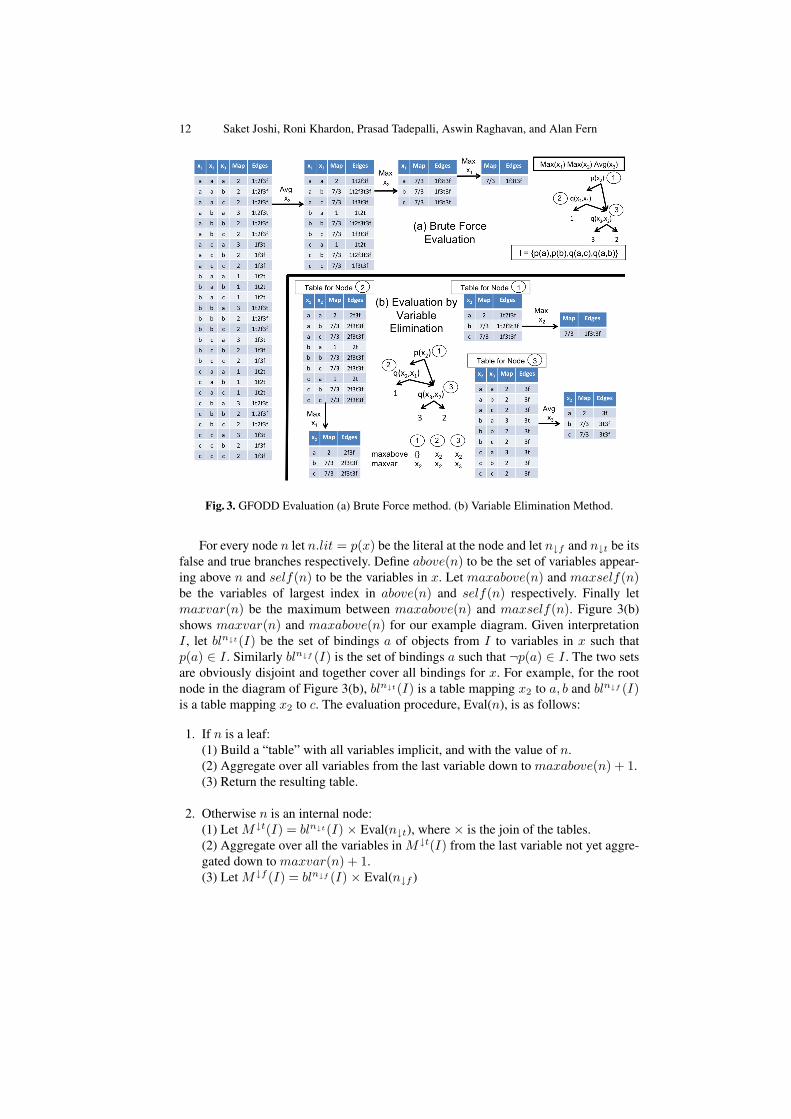
Given a diagram B = (aggregatexf(x)), an interpretation I , and a substitution ofvariables in x to objects in I , one can traverse a path to a leaf which gives the value forthat substitution. The values of all substitutions are aggregated exactly as in expressions.In particular, let the variables as ordered in the aggregation function be x1, . . . , xn.To calculate the final value, mapB(I), the semantics prescribes that we enumerate allsubstitutions of variables {xi} to objects in I and then perform the aggregation overthe variables, going from xn to x1. We can therefore think of the aggregation as if itorganizes the substitutions into blocks (with fixed value to the first k − 1 variables andall values for the k’th variable), and then aggregates the value of each block separately,repeating this from xn to x1. We call the algorithm that follows this definition directlybrute force evaluation. A detailed example is shown in Figure 3(a). To evaluate thediagram in Figure 3(a) on the interpretation shown there we enumerate all 33 = 27substitutions of 3 objects to 3 variables, obtain a value for each, and then aggregate thevalues. In the block where x1 = a, x2 = b, and x3 varies over a, b, c we get the values3, 2, 2 and an aggregated value of 7/3. This can be done for every block, and then wecan aggregate over substitutions of x2 and x1. The final value in this case is 7/3.

Any binary operation op over real values can be generalized to open and closed ex-pressions in a natural way. If f1 and f2 are two closed expressions, f1 op f2 representsthe function which maps each interpretation w to f1(w) op f2(w). We follow the gen-eral convention of using⊕ and⊗ to denote + and× respectively when they are appliedto expressions. This provides a definition but not an implementation of binary opera-tions over expressions. The work in [8] showed that if the binary operation is safe, i.e., itdistributes with respect to all aggregation operators, then there is a simple algorithm (theApply procedure) implementing the binary operation over expressions. For example ⊕is safe w.r.t. max aggregation, and it is easy to see that (maxx f(x))⊕ (maxx g(x)) =maxx maxy f(x) + g(y), and the open formula portion (diagram portion) of the result


Fig. 1. IC Dynamics and Regression (a) An example GFODD. (b) TVD for empty(s) under thedeterministic action unload(t∗, s∗). (c) Regressing the GFODD of (a) over unload(t∗, s∗). (d)Object Maximization. In these diagrams and throughout the paper, left-going edges represent thetrue branch out of the node and right-going edges represent the false branch.

can be calculated directly from the open expressions f(x) and g(y). The Apply pro-cedure [20, 8] calculates a diagram representing f(x) + g(y) using operations over thegraphs representing f(x) and g(y). Note that we need to standardize apart, as in therenaming of g(x) to g(y) for such operations.SDP for Relational MDPs: SDP provides a symbolic implementation of the value it-eration update of Eq (1) that avoids state enumeration implicit in that equation. TheSDP algorithm of [8] generalizing [3] calculates one iteration of value iteration as fol-lows. As input we get (as GFODDs) closed expressions Vn, R (we use Figure 1(a) asthe reward in the example below), and open expressions for the probabilistic choice ofactions Pr(Aj(x)|A(x)) and for the dynamics of deterministic action variants.

The action dynamics are specified by providing a diagram (called truth value dia-gram or TVD) for each variant Aj(x) and predicate template p(y). The correspondingTVD, T (Aj(x), p(y)), is an open expression that specifies the truth value of p(y) in thenext state when Aj(x) has been executed in the current state. Figure 1(b) shows theTVD of unload(t∗, s∗) for predicates empty(s). Note that in contrast to other repre-sentations of planning operators (but similar to the successor state axioms of [3]) TVDsspecify the truth value after the action and not the change in truth value. Since unload isdeterministic we have only one variant and Pr(Aj(x)|A(x)) = 1. We illustrate prob-abilistic actions in the next section. Following [20, 8] we require that Pr(Aj(x)|A(x))and T (Aj(x), p(y)) have no aggregations and cannot introduce new variables, that is,the first refers to x only and the second to x and y but no other variables. This im-plies that the regression and product terms in the algorithm below do not change theaggregation function and therefore enables the analysis of the algorithm.

The SDP algorithm of [8] implements Eq (1) using the following 4 steps. We denotethis as Vi+1 = SDP 1(Vi).


1. Regression: The n step-to-go value function Vn is regressed over every determin-istic variant Aj(x) of every action A(x) to produce Regr(Vn, Aj(x)). Regressionis conceptually similar to goal regression in deterministic planning but it needs tobe done for all (potentially exponential number of) paths in the diagram, each ofwhich can be thought of as a goal in the planning context. This can be done effi-ciently by replacing every atom in the open formula portion of Vn (a node in theGFODD representation) by its corresponding TVD without changing the aggrega-tion function.Figure 1(c) illustrates the process of block replacement for the diagram of part (a).Note that tin() is not affected by the action. Therefore its TVDs simply repeatsthe predicate value, and the corresponding node is unchanged by block replace-ment. Therefore, in this example, we are effectively replacing only one node withits TVD. The TVD leaf valued 1 is connected to the left child (true branch) of thenode and the 0 leaf is connected to the right child (false branch). To maintain thediagrams sorted we must in fact use a different implementation than block replace-ment; the implementation does not affect the constructions or proofs in the paperand we therefore refer the reader to [20] for the details.

2. Add Action Variants: The Q-function QA(x)Vn

= R ⊕ [γ ⊗ ⊕j(Pr(Aj(x)) ⊗Regr(Vn, Aj(x)))] for each action A(x) is generated by combining regressed dia-grams using the binary operations ⊕ and ⊗ over expressions.Recall that probability diagrams do not refer to additional variables. The multipli-cation can therefore be done directly on the open formulas without changing theaggregation function. As argued by [20], to guarantee correctness, both summationsteps (⊕j and R⊕ steps) must standardize apart the functions before adding them.

3. Object Maximization: Maximize over the action parameters QA(x)Vn

to produceQAVn

for each action A(x), thus obtaining the value achievable by the best groundinstantiation of A(x) in each state. This step is implemented by converting actionparameters x in QA(x)

Vnto variables, each associated with the max aggregation op-

erator, and appending these operators to the head of the aggregation function.For example, if object maximization were applied to the diagram of Figure 1(c)(we skipped some intermediate steps) then t∗, s∗ would be replaced with variablesand given max aggregation so that the aggregation is as shown in part (d) of thefigure. Therefore, in step 2, t∗, s∗ are constants (temporarily added to the logicallanguage) referring to concrete objects in the world, and in step 3 we turn them intovariables and specify the aggregation function for them.

4. Maximize over Actions: The n+ 1 step-to-go value function Vn+1 = maxAQAVn,

is generated by combining the diagrams using the binary operation max over ex-pressions.

The main advantage of this approach is that the regression operation, and the binaryoperations over expressions⊕,⊗, max can be performed symbolically and therefore thefinal value function output by the algorithm is a closed expression in the same language.We therefore get a completely symbolic form of value iteration. Several instantiations ofthis idea have been implemented [11, 6, 18, 20]. Except for the work of [8, 18] previouswork has handled only max aggregation. Previous work [8] relies on the fact that thebinary operations ⊕, ⊗, and max are safe with respect to max,min aggregation to


provide a GFODD based SDP algorithm for problems where the reward function hasmax and min aggregations . In this paper we use reward functions with max and avgaggregation. The binary operations ⊕ and ⊗ are safe with respect to avg but the binaryoperation max is not. For example 2 + avg{1, 2, 3} = avg{2 + 1, 2 + 2, 2 + 3} butmax{2, avg{1, 2, 3}} 6= avg{max{2, 1},max{2, 2},max{2, 3}}. To address this issuewe introduce a new implementation for this case in the next section.

3 Model and Algorithms for Service Domains

We now proceed to describe our extensions to SDP to handle exogenous events. Exoge-nous events refer to spontaneous changes to the state without agent action. Our mainmodeling assumption, denoted A1, is that we have object-centered exogenous actionsthat are automatically taken in every time step. In particular, for every object i in the do-main we have action E(i) that acts on object i and the conditions and effects of {E(i)}are such that they are mutually non-interfering: given any state s, all the actions {E(i)}are applied simultaneously, and this is equivalent to their sequential application in anyorder. We use the same GFODD action representation described in the previous sectionto capture the dynamics of E(i).Example: IC Domain. We use a simple version of the inventory control domain (IC)as a running example, and for some of the experimental results. In IC the objects are adepot, a truck and a number of shops. A shop can be empty or full, i.e., the inventory hasonly two levels and the truck can either be at the depot or at a shop. The reward is thefraction (average) of non-empty shops. Agent actions are deterministic and they capturestock replacement. In particular, a shop can be filled by unloading inventory from thetruck in one step. The truck can be loaded in a depot and driven from any location (shopor depot) to any location in one step. The exogenous action E(i) has two variants; thesuccess variant Esucc(i) (customer arrives at shop i, and if non-empty the inventorybecomes empty) occurs with probability 0.4 and the fail variant Efail(i) (no customer,no changes to state) occurs with probability 0.6. Figure 2 parts (a)-(d) illustrate themodel for IC and its GFODD representation. In order to facilitate the presentation ofalgorithmic steps, Figure 2(e) shows a slightly different reward function (continuingprevious examples) that is used as the reward in our running example.

For our analysis we make two further modeling assumptions. A2: we assume thatexogenous action E(i) can only affect unary properties of the object i. To simplifythe presentation we consider a single such predicate sp(i) that may be affected, but anynumber of such predicates can be handled. In IC, the special predicate sp(i) is empty(i)specifying whether the shop is empty. A3: we assume that sp() does not appear in theprecondition of any agent action. It follows that E(i) only affects sp(i) and that sp(i)can appear in the precondition of E(i) but cannot appear in the precondition of anyother action.

3.1 The Template Method

Extending SDP to handle exogenous events is complicated because the events dependon the objects in the domain and on their number and exact solutions can result in com-plex expressions that require counting formulas over the domain [17, 15]. A possible


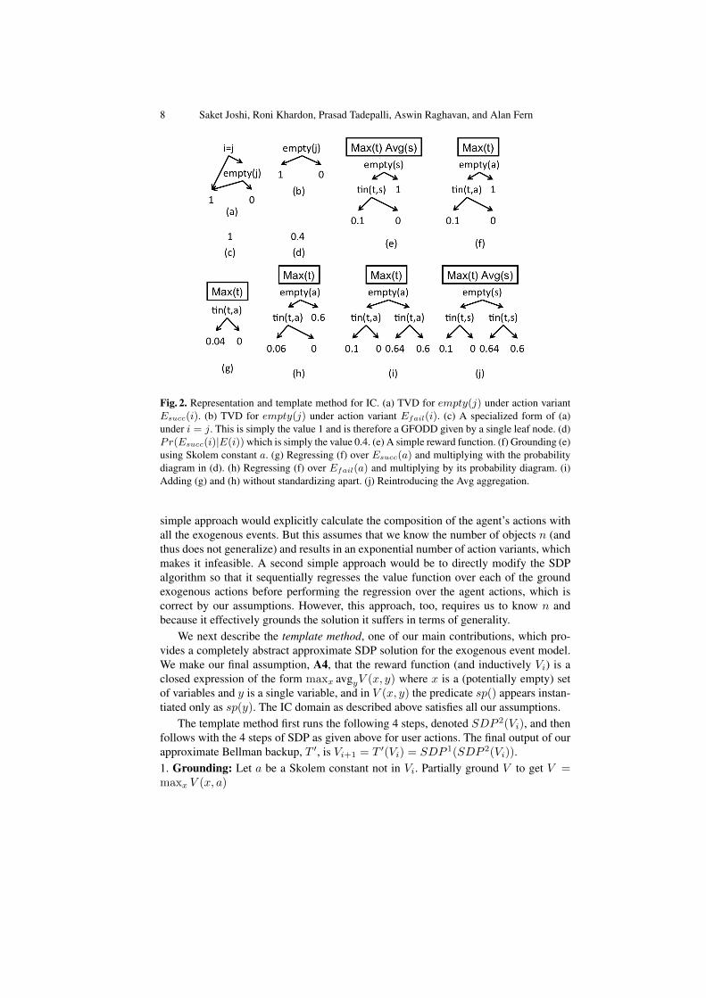
Fig. 2. Representation and template method for IC. (a) TVD for empty(j) under action variantEsucc(i). (b) TVD for empty(j) under action variant Efail(i). (c) A specialized form of (a)under i = j. This is simply the value 1 and is therefore a GFODD given by a single leaf node. (d)Pr(Esucc(i)|E(i)) which is simply the value 0.4. (e) A simple reward function. (f) Grounding (e)using Skolem constant a. (g) Regressing (f) over Esucc(a) and multiplying with the probabilitydiagram in (d). (h) Regressing (f) over Efail(a) and multiplying by its probability diagram. (i)Adding (g) and (h) without standardizing apart. (j) Reintroducing the Avg aggregation.

simple approach would explicitly calculate the composition of the agent’s actions withall the exogenous events. But this assumes that we know the number of objects n (andthus does not generalize) and results in an exponential number of action variants, whichmakes it infeasible. A second simple approach would be to directly modify the SDPalgorithm so that it sequentially regresses the value function over each of the groundexogenous actions before performing the regression over the agent actions, which iscorrect by our assumptions. However, this approach, too, requires us to know n andbecause it effectively grounds the solution it suffers in terms of generality.

We next describe the template method, one of our main contributions, which pro-vides a completely abstract approximate SDP solution for the exogenous event model.We make our final assumption, A4, that the reward function (and inductively Vi) is aclosed expression of the form maxx avgyV (x, y) where x is a (potentially empty) setof variables and y is a single variable, and in V (x, y) the predicate sp() appears instan-tiated only as sp(y). The IC domain as described above satisfies all our assumptions.

The template method first runs the following 4 steps, denoted SDP 2(Vi), and thenfollows with the 4 steps of SDP as given above for user actions. The final output of ourapproximate Bellman backup, T ′, is Vi+1 = T ′(Vi) = SDP 1(SDP 2(Vi)).1. Grounding: Let a be a Skolem constant not in Vi. Partially ground V to get V =maxx V (x, a)


2. Regression: The function V is regressed over every deterministic variant Ej(a) ofthe exogenous action centered at a to produce Regr(V,Ej(a)).3. Add Action Variants: The value function V = ⊕j(Pr(Ej(a)) ⊗ Regr(V,Ej(a)))is updated. As in SDP 1, multiplication is done directly on the open formulas withoutchanging the aggregation function. Importantly, in contrast with SDP 1, here we do notstandardize apart the functions when performing ⊕j . This leads to an approximation.4. Lifting: Let the output of the previous step be V = maxxW (x, a). Return V =maxx avgyW (x, y).

Thus, the algorithm grounds V using a generic object for exogenous actions, it thenperforms regression for a single generic exogenous action, and then reintroduces theaggregation. Figure 2 parts (e)-(j) illustrate this process.

We now show that our algorithm provides a monotonic lower bound on the valuefunction. The crucial step is the analysis of SDP 2(Vi). We have:

Lemma 1. Under assumptions A1, A2, A4 the value function calculated by SDP 2(Vi)is a lower bound on the value of regression of Vi through all exogenous actions.

Due to space constraints the complete proof is omitted and we only provide a sketch.This proof and other omitted details can be found in the full version of this paper [10].

Proof. (sketch) The main idea in the proof is to show that, under our assumptions, theresult of our algorithm is equivalent to sequential regression of all exogenous actions,where in each step the action variants are not standardized apart.

Recall that the input value function Vi has the form V = maxx avgyV (x, y) =maxx 1

n [V (x, 1)+V (x, 2)+ . . .+V (x, n)]. To establish this relationship we show thatafter the sequential algorithm regressesE(1), . . . , E(k) the intermediate value functionhas the form maxx 1

n [W (x, 1)+W (x, 2)+. . .+W (x, k)+V (x, k+1)+. . .+V (x, n)].That is, the first k portions change in the same structural manner into a diagram W andthe remaining portions retain their original form V . In addition, W (x, `) is the resultof regressing V (x, `) through E(`) which is the same form as calculated by step 3of the template method. Therefore, when all E(`) have been regressed, the result isV = maxx avgyW (x, y) which is the same as the result of the template method.

The sequential algorithm is correct by definition when standardizing apart but yieldsa lower bound when not standardizing apart. This is true because for any functions f1

and f2 we have [maxx1 avgy1f1(x1, y1)] + [maxx2 avgy2f

2(x2, y2)] ≥ maxx[avgy1f1(x, y1)+avgy2f

2(x, y2)] = maxx avgy[(f1(x, y)+f2(x, y))] where the last equality

holds because y1 and y2 range over the same set of objects. Therefore, if f1 and f2

are the results of regression for different variants from step 2, adding them withoutstandardizing apart as in the last equation yields a lower bound. ut

The lemma requires that Vi used as input satisfies A4. If this holds for the rewardfunction, and if SDP 1 maintains this property then A4 holds inductively for all Vi.Put together this implies that the template method provides a lower bound on the trueBellman backup. It therefore remains to show how SDP 1 can be implemented formaxx avgy aggregation and that it maintains the form A4.

First consider regression. If assumption A3 holds, then our algorithm using regres-sion through TVDs does not introduce new occurrences of sp() into V . Regression also


does not change the aggregation function. Similarly, the probability diagrams do notintroduce sp() and do not change the aggregation function. Therefore A4 is maintainedby these steps. For the other steps we need to discuss the binary operations ⊕ and max.

For ⊕, using the same argument as above, we see that [maxx1 avgy1f1(x1, y1)] +

[maxx2 avgy2f2(x2, y2)] = maxx1 maxx2 [avgy f

1(x1, y)+ f2(x2, y)] and therefore itsuffices to standardize apart the x portion but y can be left intact and A4 is maintained.

Finally, recall that we need a new implementation for the binary operation maxwith avg aggregation. This can be done as follows: to perform max{[maxx1 avgy1f1(x1, y1)], [maxx2 avgy2f

2(x2, y2)]} we can introduce two new variables z1, z2 andwrite the expression: “maxz1,z2 maxx1 maxx2 avgy1avgy2 (if z1 = z2 then f1(x1, y1)else f2(x2, y2))”. This is clearly correct whenever the interpretation has at least two ob-jects because z1, z2 are unconstrained. Now, because the branches of the if statement aremutually exclusive, this expression can be further simplified to “maxz1,z2 maxx avgy(if z1 = z2 then f1(x, y) else f2(x, y))”. The implementation uses an equality nodeat the root with label z1 = z2, and hangs f1 and f2 at the true and false branches.Crucially it does not need to standardize apart the representation of f1 and f2 and thusA4 is maintained. This establishes that the approximation returned by our algorithm,T ′[Vi], is a lower bound of the true Bellman backup T [Vi].

An additional argument (details available in [10]) shows that this is a monotoniclower bound, that is, for all i we have T [Vi] ≥ Vi where T [V ] is the true Bellmanbackup. It is well known (e.g., [12]) that if this holds then the value of the greedypolicy w.r.t. Vi is at least Vi (this follows from the monotonicity of the policy updateoperator Tπ). The significance is, therefore, that Vi provides an immediate certificate onthe quality of the resulting greedy policy. Recall that T ′[V ] is our approximate backup,V0 = R and Vi+1 = T ′[Vi]. We have:

Theorem 1. When assumptions A1, A2, A3, A4 hold and the reward function is non-negative we have for all i: Vi ≤ Vi+1 = T ′[Vi] ≤ T [Vi] ≤ V ∗.

As mentioned above, although the assumptions are required for our analysis, thealgorithm can be applied more widely. Assumptions A1 and A4 provide our basic mod-eling assumption per object centered exogenous events and additive rewards. It is easyto generalize the algorithm to have events and rewards based on object tuples insteadof single objects. Similarly, while the proof fails when A2 (exogenous events only af-fect special unary predicates) is violated the algorithm can be applied directly withoutmodification. When A3 does not hold, sp() can appear with multiple arguments and thealgorithm needs to be modified. Our implementation introduces an additional approx-imation and at iteration boundary we unify all the arguments of sp() with the averagevariable y. In this way the algorithm can be applied inductively for all i. These exten-sions of the algorithm are demonstrated in our experiments.Relation to Straight Line Plans: The template method provides symbolic way to cal-culate a lower bound on the value function. It is interesting to consider what kind oflower bound this provides. Recall that the straight line plan approximation (see e.g.,discussion in [2]) does not calculate a policy and instead at any state it seeks the bestlinear plan with highest expected reward. As the next observation argues (proof avail-able in [10]) the template method provides a related approximation. We note, however,


that unlike previous work on straight line plans our computation is done symbolicallyand calculates the approximation for all start states simultaneously.

Observation 1. The template method provides an approximation that is related to thevalue of the best straight line plan. When there is only one deterministic agent actiontemplate we get exactly the value of the straight line plan. Otherwise, the approximationis bounded between the value of the straight line plan and the optimal value.

4 Evaluation and Reduction of GFODDs

The symbolic operations in the SDP algorithm yield diagrams that are redundant in thesense that portions of them can be removed without changing the values they compute.Recently, [8, 7] introduced the idea of model checking reductions to compress such dia-grams. The basic idea is simple. Given a set of “focus states” S, we evaluate the diagramon every interpretation in S. Any portion of the diagram that does not “contribute” tothe final value in any of the interpretations is removed. The result is a diagram which isexact on the focus states, but may be approximate on other states. We refer the readerto [8, 7] for further motivation and justification. In that work, several variants of thisidea have been analyzed formally (for max and min aggregation), have been shownto perform well empirically (for max aggregation), and methods for generating S viarandom walks have been developed. In this section we develop the second contributionof the paper, providing an efficient realization of this idea for maxx avgy aggregation.

The basic reduction algorithm, which we refer to below as brute force model check-ing for GFODDs, is: (1) Evaluate the diagram on each example in our focus set Smarking all edges that actively participate in generating the final value returned for thatexample. Because we have maxx avgy this value is given by the “winner” of max ag-gregation. This is a block of substitutions that includes one assignment to x and allpossible assignments to y. For each such block collect the set of edges traversed by anyof the substitutions in the block. When picking the max block, also collect the edgestraversed by that block, breaking ties by lexicographic ordering over edge sets. (2) Takethe union of marked edges over all examples, connecting any edge not in this set to 0.

Consider again the example of evaluation in Figure 3(a), where we assigned nodeidentifiers 1,2,3. We identify edges by their parent node and its branch so that the left-going edge from the root is edge 1t. In this case the final value 7/3 is achieved bymultiple blocks of substitutions, and two distinct sets of edges 1t2f3t3f and 1f3t3f .Assuming 1<2<3 and f<t, 1f3t3f is lexicographically smaller and is chosen as themarked set. This process is illustrated in the tables of Figure 3(a). Referring to thereduction procedure, if our focus set S includes only this interpretation, then the edges1t, 2t, 2f will be redirected to the value 0.Efficient Model Evaluation and Reduction: We now show that the same process ofevaluation and reduction can be implemented more efficiently. The idea, taking inspira-tion from variable elimination, is that we can aggregate some values early while calcu-lating the tables. However, our problem is more complex than standard variable elimi-nation and we require a recursive computation over the diagram.


Fig. 3. GFODD Evaluation (a) Brute Force method. (b) Variable Elimination Method.

For every node n let n.lit = p(x) be the literal at the node and let n↓f and n↓t be itsfalse and true branches respectively. Define above(n) to be the set of variables appear-ing above n and self(n) to be the variables in x. Let maxabove(n) and maxself(n)be the variables of largest index in above(n) and self(n) respectively. Finally letmaxvar(n) be the maximum between maxabove(n) and maxself(n). Figure 3(b)shows maxvar(n) and maxabove(n) for our example diagram. Given interpretationI , let bln↓t(I) be the set of bindings a of objects from I to variables in x such thatp(a) ∈ I . Similarly bln↓f (I) is the set of bindings a such that ¬p(a) ∈ I . The two setsare obviously disjoint and together cover all bindings for x. For example, for the rootnode in the diagram of Figure 3(b), bln↓t(I) is a table mapping x2 to a, b and bln↓f (I)is a table mapping x2 to c. The evaluation procedure, Eval(n), is as follows:

1. If n is a leaf:(1) Build a “table” with all variables implicit, and with the value of n.(2) Aggregate over all variables from the last variable down to maxabove(n) + 1.(3) Return the resulting table.

2. Otherwise n is an internal node:(1) Let M↓t(I) = bln↓t(I) × Eval(n↓t), where × is the join of the tables.(2) Aggregate over all the variables in M↓t(I) from the last variable not yet aggre-gated down to maxvar(n) + 1.(3) Let M↓f (I) = bln↓f (I) × Eval(n↓f )


(4) Aggregate over all the variables in M↓f (I) from the last variable not yet aggre-gated down to maxvar(n) + 1.(5) Let M = M↓t(I) ∪M↓f (I).(6) Aggregate over all the variables in M from the last variable not yet aggregateddown to maxabove(n) + 1.(7) Return node table M .

We note several improvements for this algorithm and its application for reductions,all of which are applicable and used in our experiments. (I1) We implement the aboverecursive code using dynamic programming to avoid redundant calls. (I2) When anaggregation operator is idempotent, i.e., op{a, . . . , a} = a, aggregation over implicitvariables does not change the table, and the implementation is simplified. This holds formax and avg aggregation. (I3) In the case of maxx avgy aggregation the procedure ismade more efficient (and closer to variable elimination where variable order is flexible)by noting that, within the set of variables x, aggregation can be done in any order.Therefore, once y has been aggregated, any variable that does not appear above node ncan be aggregated at n. (I4) The recursive algorithm can be extended to collect edge setsfor winning blocks by associating them with table entries. Leaf nodes have empty edgesets. The join step at each node adds the corresponding edge (for true or false child) foreach entry. Finally, when aggregating an average variable we take the union of edges,and when aggregating a max variable we take the edges corresponding to the winningvalue, breaking ties in favor of the lexicographically smaller set of edges.

A detailed example of the algorithm is given in Figure 3(b) where the evaluationis on the same interpretation as in part (a). We see that node 3 first collects a tableover x2, x3 and that, because x3 is not used above, it already aggregates x3. The joinstep for node 2 uses entries (b, a) and (c, a) for (x1, x2) from the left child and otherentries from the right child. Node 2 collects the entries and (using I3) aggregates x1

even though x2 appears above. Node 1 then similarly collects and combines the tablesand aggregates x2. The next theorem is proved by induction over the structure of theGFODD (details available in [10]).

Theorem 2. The value and max block returned by the modified Eval procedure areidentical to the ones returned by the brute force method.

5 Experimental Validation

In this section we present an empirical demonstration of our algorithms. To that endwe implemented our algorithms in Prolog as an extension of the FODD-PLANNER[9], and compared it to SPUDD [5] and MADCAP [19] that take advantage of propo-sitionally factored state spaces, and implement VI using propositional algebraic deci-sion diagrams (ADD) and affine ADDs respectively. For SPUDD and MADCAP, thedomains were specified in the Relational Domain Description Language (RDDL) andtranslated into propositional descriptions using software provided for the IPPC 2011planning competition [16]. All experiments were run on an Intel Core 2 Quad CPU @2.83GHz. Our system was given 3.5Gb of memory and SPUDD and MADCAP weregiven 4Gb.


Fig. 4. Experimental Results

We tested all three systems on the IC domain as described above where shops andtrucks have binary inventory levels (empty or full). We present results for the IC domain,because it satisfies all our assumptions and because the propositional systems fare betterin this case. We also present results for a more complex IC domain (advanced IC orAIC below) where the inventory can be in one of 3 levels 0,1 and 2 and a shop canhave one of 2 consumption rates 0.3 and 0.4. AIC does not satisfy assumption A3.As the experiments show, even with this small extension, the combinatorics render thepropositional approach infeasible. In both cases, we constructed the set of focus statesto include all possible states over 2 shops. This provides exact reduction for states with2 shops but the reduction is approximate for larger states as in our experiments.

Figure 4 summarizes our results, which we discuss from left to right and top tobottom. The top left plot shows runtime as a function of iterations for AIC and illustratesthat the variable elimination method is significantly faster than brute force evaluationand that it enables us to run many more iterations. The top right plot shows the totaltime (translation from RDDL to a propositional description and off-line planning for 10iterations of VI) for the 3 systems for one problem instance per size for AIC. SPUDDruns out of memory and fails on more than 4 shops and MADCAP can handle at most 5


shops. Our planning time (being domain size agnostic) is constant. Runtime plots for ICare omitted but they show a similar qualitative picture, where the propositional systemsfail with more than 8 shops for SPUDD and 9 shops for MADCAP.

The middle two plots show the cost of using the policies, that is, the on-line execu-tion time as a function of increasing domain size in test instances. To control run time forour policies we show the time for the GFODD policy produced after 4 iterations, whichis sufficient to solve any problem in IC and AIC.4 On-line time for propositional sys-tems is fast for the domain sizes they solve, but our system can solve problems of muchlarger size (recall that the state space grows exponentially with the number of shops).The bottom two plots show the total discounted reward accumulated by each system (aswell as a random policy) on 15 randomly generated problem instances averaged over30 runs. In both cases all algorithms are significantly better than the random policy. InIC our approximate policy is not distinguishable from the optimal (SPUDD). In AICthe propositional policies are slightly better (differences are statistically significant). Insummary, our system provides a non-trivial approximate policy but is sub-optimal insome cases, especially in AIC where A3 is violated. On the other hand its offline plan-ning time is independent of domain size, and it can solve instances that cannot be solvedby the propositional systems.

6 Conclusions

The paper presents service domains as an abstraction of planning problems with ad-ditive rewards and with multiple simultaneous but independent exogenous events. Weprovide a new relational SDP algorithm and the first complete analysis of such an al-gorithm with provable guarantees. In particular our algorithm, the template method, isguaranteed to provide a monotonic lower bound on the true value function under sometechnical conditions. We have also shown that this lower bound lies between the valueof straight line plans and the true value function. As a second contribution we intro-duce new evaluation and reduction algorithms for the GFODD representation, that inturn facilitate efficient implementation of the SDP algorithm. Preliminary experimentsdemonstrate the viability of our approach and that our algorithm can be applied even insituations that violate some of the assumptions used in the analysis. The paper providesa first step toward analysis and solutions of general problems with exogenous events byfocusing on a well defined subset of such models. Identifying more general conditionsfor existence of compact solutions, representations for such solutions, and associated al-gorithms is an important challenge for future work. In addition, the problems involvedin evaluation and application of diagrams are computationally demanding. Techniquesto speed up these computations are an important challenge for future work.

Acknowledgements This work was partly supported by NSF under grants IIS-0964457and IIS-0964705 and the CI fellows award for Saket Joshi. Most of this work was donewhen Saket Joshi was at Oregon State University.

4 Our system does not achieve structural convergence because the reductions are not comprehen-sive. We give results at 4 iterations as this is sufficient for solving all problems in this domain.With more iterations, our policies are larger and their execution is slower.


References

1. Bahar, R., Frohm, E., Gaona, C., Hachtel, G., Macii, E., Pardo, A., Somenzi, F.: Algebraicdecision diagrams and their applications. In: Proceedings of the IEEE/ACM InternationalConference on Computer-Aided Design. pp. 188–191 (1993)

2. Boutilier, C., Dean, T., Hanks, S.: Decision-theoretic planning: Structural assumptions andcomputational leverage. Journal of Artificial Intelligence Research 11, 1–94 (1999)

3. Boutilier, C., Reiter, R., Price, B.: Symbolic dynamic programming for first-order MDPs.In: Proceedings of the International Joint Conference of Artificial Intelligence. pp. 690–700(2001)

4. Guestrin, C., Koller, D., Parr, R., Venkataraman, S.: Efficient solution algorithms for factoredMDPs. Journal of Artificial Intelligence Research 19, 399–468 (2003)

5. Hoey, J., St-Aubin, R., Hu, A., Boutilier, C.: SPUDD: Stochastic planning using decisiondiagrams. In: Proceedings of Uncertainty in Artificial Intelligence. pp. 279–288 (1999)

6. Holldobler, S., Karabaev, E., Skvortsova, O.: FluCaP: a heuristic search planner for first-order MDPs. Journal of Artificial Intelligence Research 27, 419–439 (2006)

7. Joshi, S., Kersting, K., Khardon, R.: Self-Taught decision theoretic planning with first-orderdecision diagrams. In: Proceedings of the International Conference on Automated Planningand Scheduling. pp. 89–96 (2010)

8. Joshi, S., Kersting, K., Khardon, R.: Decision theoretic planning with generalized first orderdecision diagrams. Artificial Intelligence 175, 2198–2222 (2011)

9. Joshi, S., Khardon, R.: Probabilistic relational planning with first-order decision diagrams.Journal of Artificial Intelligence Research 41, 231–266 (2011)

10. Joshi, S., Khardon, R., Tadepalli, P., Raghavan, A., Fern, A.: Solving relationalMDPs with exogenous events and additive rewards. CoRR abs/1306.6302 (2013),http://arxiv.org/abs/1306.6302

11. Kersting, K., van Otterlo, M., De Raedt, L.: Bellman goes relational. In: Proceedings of theInternational Conference on Machine Learning. pp. 465–472 (2004)

12. McMahan, H.B., Likhachev, M., Gordon, G.J.: Bounded real-time dynamic programming:RTDP with monotone upper bounds and performance guarantees. In: Proceedings of theInternational Conference on Machine Learning. pp. 569–576 (2005)

13. Puterman, M.L.: Markov Decision Processes: Discrete Stochastic Dynamic Programming.Wiley (1994)

14. Russell, S., Norvig, P.: Artificial Intelligence: A Modern Approach. Prentice Hall Series inArtificial Intelligence (2002)

15. Sanner, S.: First-order decision-theoretic planning in structured relational environments.Ph.D. thesis, University of Toronto (2008)

16. Sanner, S.: Relational dynamic influence diagram language (RDDL): Language descriptionhttp://users.cecs.anu.edu.au/∼sanner/IPPC 2011/RDDL.pdf (2010)

17. Sanner, S., Boutilier, C.: Approximate solution techniques for factored first-order MDPs. In:Proceedings of the International Conference on Automated Planning and Scheduling. pp.288–295 (2007)

18. Sanner, S., Boutilier, C.: Practical solution techniques for first-order MDPs. Artificial Intel-ligence 173, 748–788 (2009)

19. Sanner, S., Uther, W., Delgado, K.: Approximate dynamic programming with affine ADDs.In: Proceeding of the International Conference on Autonomous Agents and Multiagent Sys-tems. pp. 1349–1356 (2010)

20. Wang, C., Joshi, S., Khardon, R.: First-Order decision diagrams for relational MDPs. Journalof Artificial Intelligence Research 31, 431–472 (2008)

solving relational mdps with exogenous events and additive

Documents