solving hard combinatorial problems: a research …ted/files/talks/pmcs02.pdfsolving hard...
TRANSCRIPT

Solving Hard Combinatorial Problems:A Research Overview
Ted Ralphs
Department of Industrial and Systems EngineeringLehigh University, Bethlehem, PA
http://www.lehigh.edu/˜tkr2

Solving Hard Combinatorial Problems 1
Outline of Talk
• Introduction to mathematical programming
• Examples of discrete optimization problems
• Methods for discrete optimization
• Current research
1

Solving Hard Combinatorial Problems 2
What is a model?
mod·el: A schematic description of a system, theory, or phenomenon thataccounts for its known or inferred properties and may be used for furtherstudy of its characteristics.
–American Heritage Dictionary of the English Language
• Two types of models
– Concrete– Abstract
• Mathematical models
– Are abstract models– Describe the mathematical relationships among elements in a system.
2

Solving Hard Combinatorial Problems 3
Why do we model systems?
• The exercise of building a model can provide insight.
• It’s possible to do things with models that we can’t do with “the realthing.”
• Analyzing models can help us decide on a course of action.
3

Solving Hard Combinatorial Problems 4
Examples of Model Types
• Simulation Models
• Probability Models
• Financial Models
• Mathematical Programming Models
4

Solving Hard Combinatorial Problems 5
Mathematical Programming Models
• What does mathematical programming mean?
• Programming here means “planning.”
• Literally, these are “mathematical models for planning.”
• Also called optimization models.
• Essential elements
– Decision variables– Constraints– Objective Function– Parameters and Data
5

Solving Hard Combinatorial Problems 6
Forming a Mathematical Programming Model
The general form of a math programming model is:
min or max f(x1, . . . , xn)
s.t. gi(x1, . . . , xn)
≤=≥
bi
We might also require the values of the variables to belong to a discreteset X.
6

Solving Hard Combinatorial Problems 7
Solutions
• A solution is an assignment of values to variables.
• A solution can be thought of as a vector.
• A feasible solution is an assignment of values to variables such that allthe constraints are satisfied.
• The objective function value of a solution is obtained by evaluating theobjective function at the given solution.
• An optimal solution (assuming minimization) is one whose objectivefunction value is less than or equal to that of all other feasible solutions.
7

Solving Hard Combinatorial Problems 8
Types of Mathematical Programs
• The type of a math program is determined primarily by
– The form of the objective and the constraints.– The discrete set X.– Whether the input data is considered “known”.
• In this talk, we will consider linear programs.
– The objective function is linear.– The constraints are linear.– Linear programs are specified by a cost vector c ∈ Rn a constraint
matrix A ∈ Rm×n and a right-hand side vector b ∈ Rm and have theform
min cTx
s.t. Ax≤ b
8

Solving Hard Combinatorial Problems 9
Two Crude Petroleum Example
• Two Crude Petroleum distills crude from two sources:
– Saudi Arabia– Venezuela
• They have three main products:
– Gasoline– Jet fuel– Lubricants
• Yields
Gasoline Jet fuel LubricantsSaudi Arabia 0.3 barrels 0.4 barrels 0.2 barrelsVenezuela 0.4 barrels 0.2 barrels 0.3 barrels
9

Solving Hard Combinatorial Problems 10
Two Crude Petroleum Example (cont.)
• Availability and cost
Availability CostSaudi Arabia 9000 barrels $20/barrelVenezuela 6000 barrels $15/barrel
• Production Requirements (per day)
Gasoline Jet fuel Lubricants2000 barrels 1500 barrels 500 barrels
• Objective: Minimize production cost.
10

Solving Hard Combinatorial Problems 11
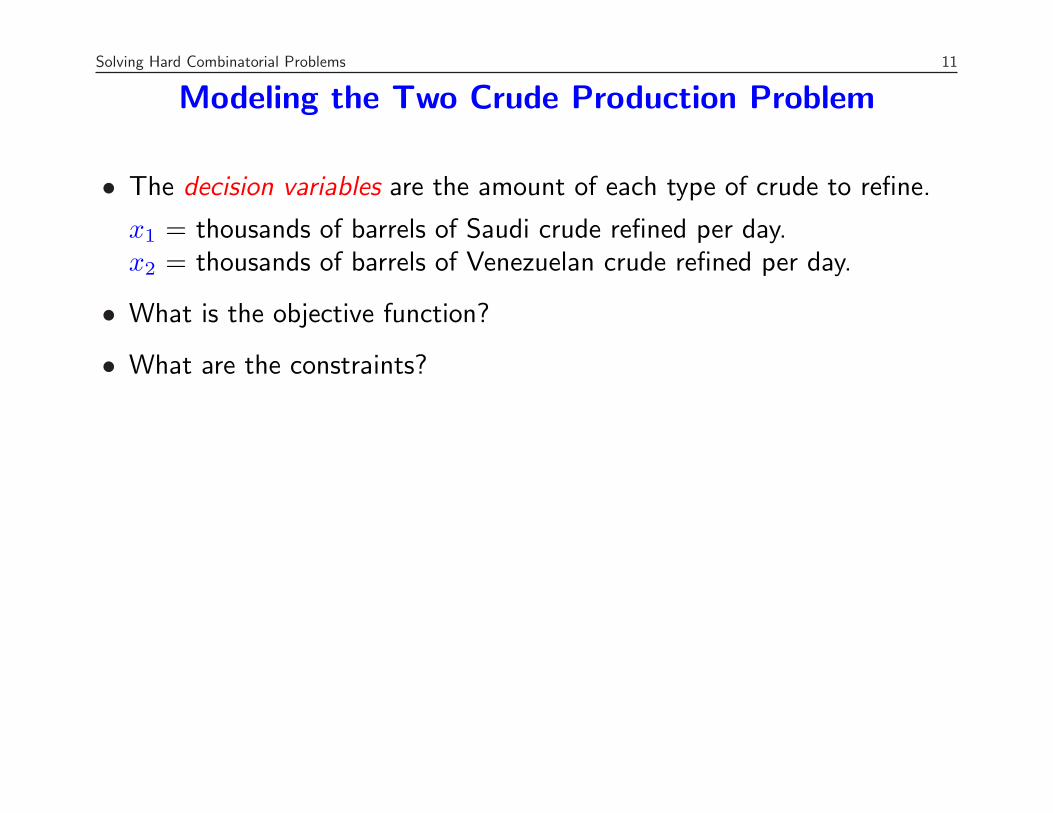
Modeling the Two Crude Production Problem
• What are the decision variables?
• What is the objective function?
• What are the constraints?
11
Solving Hard Combinatorial Problems 11
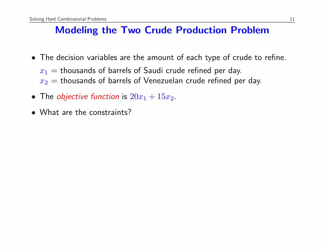
Modeling the Two Crude Production Problem
• The decision variables are the amount of each type of crude to refine.
x1 = thousands of barrels of Saudi crude refined per day.x2 = thousands of barrels of Venezuelan crude refined per day.
• What is the objective function?
• What are the constraints?
11
Solving Hard Combinatorial Problems 11
Modeling the Two Crude Production Problem
• The decision variables are the amount of each type of crude to refine.
x1 = thousands of barrels of Saudi crude refined per day.x2 = thousands of barrels of Venezuelan crude refined per day.
• The objective function is 20x1 + 15x2.
• What are the constraints?
11

Solving Hard Combinatorial Problems 11
Modeling the Two Crude Production Problem
• The decision variables are the amount of each type of crude to refine.
x1 = thousands of barrels of Saudi crude refined per day.x2 = thousands of barrels of Venezuelan crude refined per day.
• The objective function is 20x1 + 15x2.
• In words, the production constraints are
∑(yield per barrel)(barrels refined) ≥ production requirements
• In addition, we have bounds on the variables.
11
Solving Hard Combinatorial Problems 12
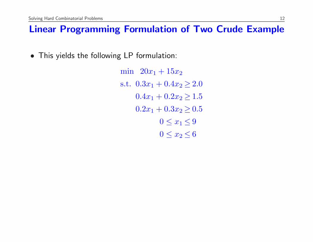
Linear Programming Formulation of Two Crude Example
• This yields the following LP formulation:
min 20x1 + 15x2
s.t. 0.3x1 + 0.4x2≥ 2.0
0.4x1 + 0.2x2≥ 1.5
0.2x1 + 0.3x2≥ 0.5
0 ≤ x1≤ 9
0 ≤ x2≤ 6
12

Solving Hard Combinatorial Problems 13
Solving Linear Programs
• Generally speaking, we can solve linear programs efficiently.
• However, in many situations, the variables must take on discrete values,usually integral values.
• These programs are called integer programs and are an example of adiscrete optimization problem.
• Integer programs can be extremely difficult to solve in practice.
• The simplest form of integer programming is combinatorial optimization.
• In a combinatorial problem, all the decisions are yes/no.
13
Solving Hard Combinatorial Problems 14
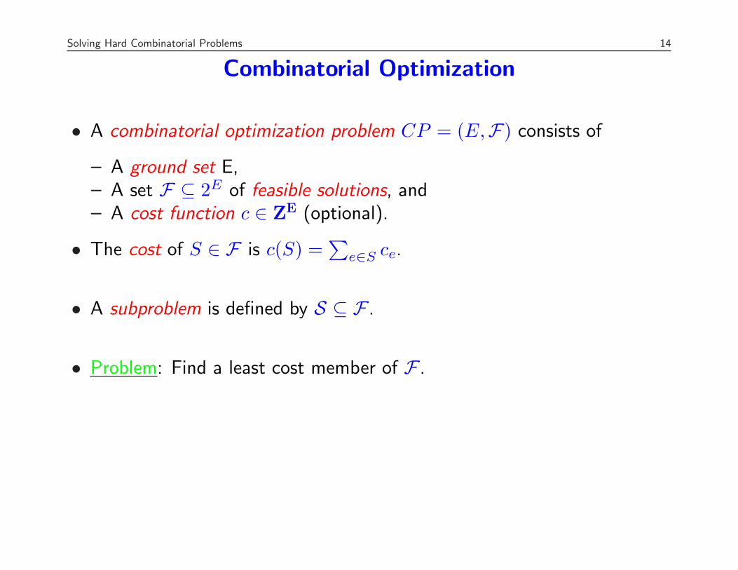
Combinatorial Optimization
• A combinatorial optimization problem CP = (E,F) consists of
– A ground set E,– A set F ⊆ 2E of feasible solutions, and– A cost function c ∈ ZE (optional).
• The cost of S ∈ F is c(S) =∑
e∈S ce.
• A subproblem is defined by S ⊆ F .
• Problem: Find a least cost member of F .
14

Solving Hard Combinatorial Problems 15
Example: Perfect Matching Problem
• We are given a set of n people that need to paired in teams of two.
• Let cij represent the “cost” of the team formed by person i and personj.
• We wish to minimize the overall cost of the pairings.
• We can represent this problem on an undirected graph G = (N,E).
• The nodes represent the people and the edges represent pairings.
• We have xe = 1 if the endpoints of e are matched, xe = 0 otherwise.
min∑
e={i,j}∈E
cexe
s.t.∑
{j|{i,j}∈E}xij = 1, ∀i ∈ N
xe ∈ {0, 1}, ∀e = {i, j} ∈ E.
15

Solving Hard Combinatorial Problems 16
Fixed-charge Problems
• In many instances, there is a fixed cost and a variable cost associatedwith a particular decision.
• Example: Fixed-charge Network Flow Problem
– We are given a directed graph G = (N, A).– There is a fixed cost cij associated with “opening” arc (i, j) (think of
this as the cost to “build” the link).– There is also a variable cost dij associated with each unit of flow along
arc (i, j).– Think of the fixed charge as the construction cost and the variable
charge as the operating cost.– We want to minimize the sum of these two costs.
16

Solving Hard Combinatorial Problems 17
Modeling the Fixed-charge Network Flow Problem
• To model the FCNFP, we associate two variables with each arc.
– xij (fixed-charge variable) indicates whether arc (i, j) is open.– fij (flow variable) represents the flow on arc (i, j).– Note that we have to ensure that fij > 0 ⇒ xij = 1.
Min∑
(i,j)∈A
cijxij + dijfij
s.t.∑
j∈O(i)
fij −∑
j∈I(i)
fji = bi ∀i ∈ N
fij ≤Cxij ∀(i, j) ∈ A
fij ≥ 0 ∀(i, j) ∈ A
xij ∈ {0, 1} ∀(i, j) ∈ A
17

Solving Hard Combinatorial Problems 18
Example: Facility Location Problem
• We are given n potential facility locations and m customers that mustbe serviced from those locations.
• There is a fixed cost cj of opening facility j.
• There is a cost dij associated with serving customer i from facility j.
• We have two sets of binary variables.
– yj is 1 if facility j is opened, 0 otherwise.– xij is 1 if customer i is served by facility j, 0 otherwise.
min
n∑
j=1
cjyj +m∑
i=1
n∑
j=1
dijxij
s.t.
n∑
j=1
xij = K ∀i
xij ≤ yj ∀i, jxij, yj ∈ {0, 1} ∀i, j
18
Solving Hard Combinatorial Problems 19
The Traveling Salesman Problem
• We are given a set of cities and a cost associated with traveling betweeneach pair of cities.
• We want to find the least cost route traveling through every city andending up back ate the starting city.
• Applications of the Traveling Salesman Problem
– Drilling Circuit Boards– Gene Sequencing
19

Solving Hard Combinatorial Problems 20
Formulating The Traveling Salesman Problem
The TSP is a combinatorial problem (E,F) whose ground set is the edgeset of a graph G = (V, E).
• V is the set of customers.
• E is the set of travel links between the customers.
A feasible solution is a permutation σ of V specifying the order of thecustomers. IP Formulation:
∑nj=1 xij = 2 ∀i ∈ N−
∑i∈Sj 6∈S
xij ≥ 2 ∀S ⊂ V, |S| > 1.
where xij is a binary variable indicating σ(i) = j.
20

Solving Hard Combinatorial Problems 21
Example Instance of the TSP
21

Solving Hard Combinatorial Problems 22
22

Solving Hard Combinatorial Problems 23
Optimal Solutions to the 48 City Problem
23
Solving Hard Combinatorial Problems 24
How hard are these problems?
• In practice, these can be extremely difficult.
• The number of possible solutions for the TSP is n! where n is the numberof cities.
• We cannot afford to enumerate all these possibilities.
• But there is no direct, efficient way to solve these problems.
24

Solving Hard Combinatorial Problems 25
How do we solve these hard problems?
• Try to reduce them to something easier
– Integer Program ⇒ Linear Program– Divide and conquer
• Use a bigger hammer
– Faster processors– More memory– Parallelism
25

Solving Hard Combinatorial Problems 26
Integer Programming
Convex hull of integer solutions
Linear programming relaxation
26

Solving Hard Combinatorial Problems 27
Cutting Plane Method
• Basic cutting plane algorithm
– Relax the integrality constraints.– Solve the relaxation. Infeasible ⇒ STOP.– If x̂ integral ⇒ STOP.– Separate x̂ from P.– No cutting planes ⇒ algorithm fails.
• The key is good separation algorithms.
27

Solving Hard Combinatorial Problems 28
Branch and Cut Methods
If the cutting plane approach fails, then we divide and conquer (branch).
28

Solving Hard Combinatorial Problems 29
Branch and Bound
• Suppose F is the feasible region for some MILP and we wish to solveminx∈F cTx.
• Consider a partition of F into subsets F1, . . . Fk. Then
minx∈F
cTx = min{1≤i≤k}
{minx∈Fi
cTx}
.
• In other words, we can optimize over each subset separately.
• Idea: If we can’t solve the original problem directly, we might be able tosolve the smaller subproblems recursively.
• Dividing the original problem into subproblems is called branching.
• Taken to the extreme, this scheme is equivalent to complete enumeration.
29

Solving Hard Combinatorial Problems 30
LP-based Branch and Bound
• In LP-based branch and bound, we first solve the LP relaxation of theoriginal problem. The result is one of the following:
1. The LP is infeasible ⇒ MILP is infeasible.2. We obtain a feasible solution for the MILP ⇒ optimal solution.3. We obtain an optimal solution to the LP that is not feasible for the
MILP ⇒ upper bound.
• In the first two cases, we are finished.
• In the third case, we must branch and recursively solve the resultingsubproblems.
30
Solving Hard Combinatorial Problems 31
Continuing the Algorithm After Branching
• After branching, we solve each of the subproblems recursively.
• Now we have an additional factor to consider.
• If the optimal solution value to the LP relaxation is greater than thecurrent upper bound, we need not consider the subproblem further.
• This is the key to the efficiency of the algorithm.
• Terminology
– If we picture the subproblems graphically, they form a search tree.– Each subproblem is linked to its parent and eventually to its children.– Eliminating a problem from further consideration is called pruning.– The act of bounding and then branching is called processing.– A subproblem that has not yet been considered is called a candidate
for processing.– The set of candidates for processing is called the candidate list.
31

Solving Hard Combinatorial Problems 32
Branch and Bound Tree
32

Solving Hard Combinatorial Problems 33
Current State of the Art
33

Solving Hard Combinatorial Problems 34
Current Research
• The theory of integer programming is fairly well developed.
• Computationally, however, these methods are very difficult to implementeffectively.
• Also, each problem requires different methods of separation.
• It is therefore extremely expensive to implement an efficient solver for anew application.
• Overcoming these challenges and developing generic solvers capable ofautomatically analyzing problem structure and performing separation isan active area of research.
• These methods also depend heavily on our ability to obtain good bounds.
• Finding new/better methods of bounding is another active research area.
• I am currently involved in research in both of these areas.
34