solutions of system of fractional partial differential ......solvability of a boundary value problem...

$: Solutions of System of Fractional Partial Differential ......solvability of a boundary value problem for a system of fractional partial differential equations in a rectangular domain$
289

Available at http://pvamu.edu/aam

Appl. Appl. Math.

ISSN: 1932-9466

Vol. 8, Issue 1 (June 2013), pp. 289 - 304

Applications and Applied Mathematics:

An International Journal (AAM)

Solutions of System of Fractional Partial Differential Equations

V. Parthiban and K. Balachandran Department of Mathematics

Bharathiar University Coimbatore - 641046

[email protected]; [email protected]

Received:April 11, 2012;Accepted: November 28, 2012

Abstract In this paper, system of fractional partial differential equation which has numerous applications in many fields of science is considered. Adomian decomposition method, a novel method is used to solve these type of equations. The solutions are derived in convergent series form which shows the effectiveness of the method for solving wide variety of fractional differential equations.

Keywords: Adomian decomposition method, Fractional partial differential equations, System

of differential equations MSC 2010 No.: 35R11, 35C10 1. Introduction

In recent years, considerable interest in fractional differential equations has been stimulated due to their numerous applications in many fields of science and engineering. Important phenomena in finance, electromagnetics, acoustics, viscoelasticity, electrochemistry and material science [Barkai et al. (2000), Meerschaert et al. (2002), Mainardi (2010), Tadjeran (2007)] are well described by differential equations of fractional order. Recently Magin et al. (2011) published a review article on the fractional signals and systems where we can find applications to control theory. Various applications of fractional calculus like image processing are found in the edited volume of Machado (2011). These applications in interdisciplinary sciences show the importance and necessity of fractional calculus. So far there have been several fundamental works on the fractional derivative and fractional differential equations, written by Oldham and Spanier (1974), Miller and Ross (1993), Podlubny (1999), Kilbas, Srivastava and Trujillo (2006) and others

290 V. Parthiban and K. Balachandran

[Samko et al. (1993), Caponetto et al. (2010), Diethelm (2010)]. Machado et al. (2010) published a review on article recent history of fractional calculus. Hernández et al. (2010) published a paper on recent developments in the theory of abstract differential equations with fractional derivatives. These works form an introduction to the theory of fractional differential equations and provide a systematic understanding of the fractional calculus such as the existence and the uniqueness of solutions, some analytical methods for solving fractional differential equations like Green’s function method, the Mellin transform method, the power series method and etc. In the literature, there exists no method that yields an exact solution for nonlinear fractional differential equations. Only approximate solutions can be derived using linearization or perturbation methods. All this motivates us to construct an efficient numerical method for fractional differential equations. The Adomian decomposition method (ADM), introduced by Adomian (1980), provides an effective procedure for finding explicit and numerical solutions of a wider and general class of differential systems representing real physical problems. This method efficiently works for initial value or boundary value problems, for linear or nonlinear, ordinary or partial differential equations, and even for stochastic systems as well. Moreover no linearization or perturbation is required in this method. In the last two decades, extensive work has been done using ADM as it provides analytical approximate solutions for nonlinear equations and considerable interest in solving fractional differential equations using ADM has been developed. Javadi (2007) proposed new ideas for the implementation of the Adomian decomposition method to solve nonlinear Volterra integral equations. The study of delay differential equations using ADM is done by Evans et al. (2005). Fakharian (2010) solves the Hamilton - Jacobi - Bellman equation arising in nonlinear optimal problem using Adomian decomposition method. It is interesting to note that Biazar et al. (2004) solved the system of first order ordinary differential equations and higher order differential equations which can be converted into a system of first order differential equations and consequently this method has been employed to study the system of integro - differential equations by Biazar (2005). Hosseini et al. (2006) introduced a simple method to determine the rate of convergence of ADM. Further they extended their earlier work of second order ordinary differential equations to higher-order ODE’s and systems of nonlinear differential equations and obtained solutions by using modified ADM in Hosseini et al. (2009). The method of Adomian decomposition was used successfully to solve a class of coupled systems of two linear second order and two nonlinear first order differential equations by Bougoffa et al. (2006). Gu and Li (2007) introduced a modified ADM to solve a system of nonlinear differential equations and also they proved that the calculating speed of the method is faster than that of the original Adomian method. Abassy (2010) considered Boussinesq equation and obtained the power series solution by using the method of improved Adomian decomposition. It should be emphasized that, to the best of our knowledge, as for as ADM for fractional differential equations is concerned, there exists a vast number of publications in the literature. Referring to all these items are beyond the scope of this paper. So let us mention briefly. System of differential equations with fractional derivatives of Riemann-Liouville and Caputo types was studied by Junsheng et al. (2007). Also they developed an algorithm to convert the multi-order fractional differential equation into a system of fractional differential equations and found their

AAM: Intern. J., Vol. 8, Issue 1 (June 2013) 291

solutions in Gejji et al. (2007). Moreover the multi-term linear and nonlinear diffusion-wave equation of fractional order is solved in Gejji (2008). Recently Saha Ray (2009) solved the spatially fractional order diffusion equation by using two-step ADM and the results obtained in his paper have been compared with the solutions obtained from ADM. Wang (2006) developed the method to obtain the solutions for the nonlinear fractional KdV-Burgers equation with time and space fractional derivatives. Hu et al. (2008) found the analytical solution of the linear fractional differential equation and shown that the solution by Adomian decomposition method is the same as the solution by the Green’s function method. Li (2009) provided a new algorithm based on ADM for fractional differential equations and compared the obtained numerical results with those obtained in the fractional Adams method. El-Sayed (2010) gave the solution to the model that describes the intermediate process between advection and dispersion via fractional derivative in the Caputo sense. In this work, we consider the system of fractional partial differential equations which is studied by Jafari et al. (2009) using homotopy analysis method. Mamchuev (2008) proved the unique solvability of a boundary value problem for a system of fractional partial differential equations in a rectangular domain and constructed the solution in closed form. Relatively Adomian (1996) presented a method of solving system of coupled nonlinear partial differential equations. In this paper, we find the solution of system of fractional partial differential equations using ADM. The graphs of their solutions are provided at the end.

2. Preliminaries

In this section, we provide some basic definitions of fractional integral and differential operators [Luchko et al. (1999)] and also we briefly describe the Adomian Decomposition Method (ADM).

Fractional Calculus

Definition 1. A real function f(t), t > 0, is said to be in the space , ,aC a R if there exists a real number p(>α)

such that 1( ) ( ),pf t t f t where 1 [0, ).f C Clearl, Cα⊂Cβ, if β ≤ α.

Definition 2. A function f(t), t > 0, is said to be in the space , 0 ,m

aC m N if ( ) .maf C

Definition 3. [Riemann - Liouville Fractional Integral Operator] The (left sided) Riemann-Liouville fractional integral of order μ ≥ 0 of a function

, 1,af C a is defined as


1 ( , ), 0, 0.1( ) 0 ( )

t f s xD ds tt

t s

Definition 4. [Caputo Fractional Derivative Operator] The (left sided) Caputo fractional derivative of f, 1,

mf C 0 ,m N is defined as

( ) ( , ), 1 , .m

C mt t m

D D f t x m m m Nt

Note that

D−μt CD

μt f(t,x)=f(t,x)−

k=0

m−1 ∂kf

∂tk(0,x)

tk

k!, m−1<μ≤m, m∈N.

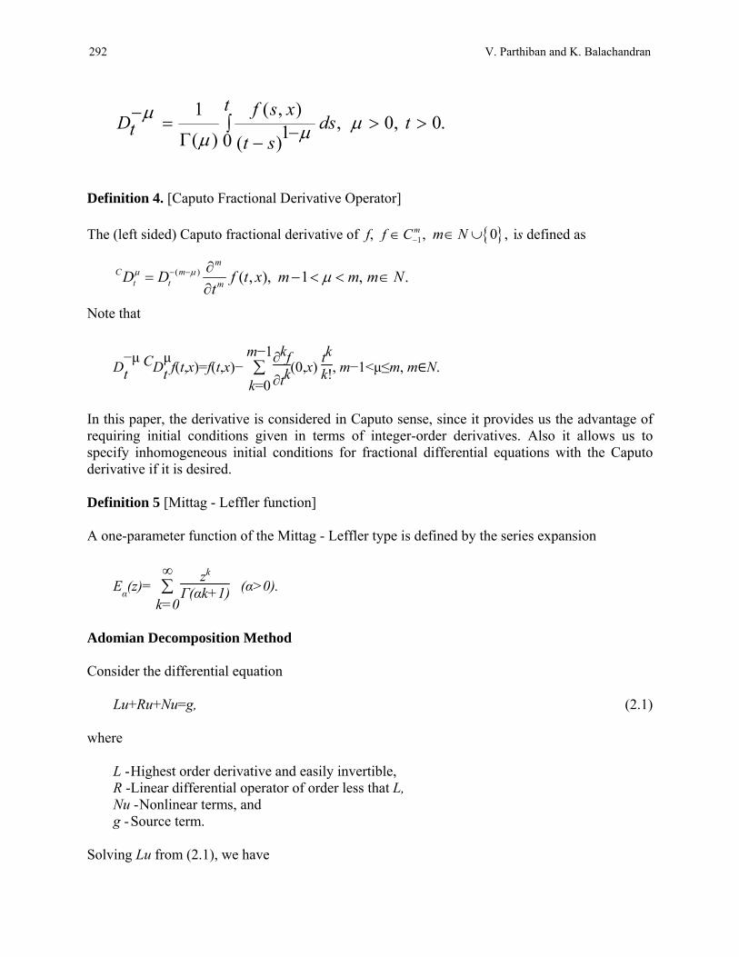
In this paper, the derivative is considered in Caputo sense, since it provides us the advantage of requiring initial conditions given in terms of integer-order derivatives. Also it allows us to specify inhomogeneous initial conditions for fractional differential equations with the Caputo derivative if it is desired. Definition 5 [Mittag - Leffler function] A one-parameter function of the Mittag - Leffler type is defined by the series expansion

Eα(z)=

k=0

∞

zk

Γ(αk+1) (α>0).

Adomian Decomposition Method Consider the differential equation

Lu+Ru+Nu=g, (2.1) where

L - Highest order derivative and easily invertible, R - Linear differential operator of order less that L, Nu - Nonlinear terms, and g - Source term.

Solving Lu from (2.1), we have


Lu=g−Ru−Nu.

Because L is invertible, the equivalent expression is

L−1Lu=L−1g−L−1Ru−L−1Nu. (2.2)

If L is a second-order operator, for example, L−1 is a two fold integration operator and

L−1Lu=u−u(0)−tu'(0), then (2.2) yields,

u=u(0)+tu'(0)+L−1g−L−1Ru−L−1Nu.

Now the solution u can be presented as a series u= n=0

∞ un with u0 identified as u(0)+tu'(0)+L−1g

and un, n>0, is to be determined. The nonlinear term Nu will be decomposed by the infinite

series of Adomian polynomials Nu= n=0

∞ An, where An is calculated using the formula

0

1( ( )) , 0,1, ,

!

n

n n

dA N n

n d

where

v(λ)= n=0

∞ λnun.

Now the series solution 0

nn

u u

to the differential equation is calculated iteratively as follows:

u0=u(0)+tu'(0)+L−1g,

un+1=−L−1(Run)−L−1(An),n≥0.

The above described method can be easily extended to a system of differential equations and the resulting equations will be of the form

ui,0 =Φi+L−1gi,

1 1

, 1 , ,( ) ( ), 0,i k i k i ku L Ru L A k


where 1 i n and Φi represent the terms arising from the given initial and boundary conditions

for a system containing n equations. 3. System of Fractional Partial Differential Equations In this section, we apply ADM to derive the solutions of a system of fractional partial differential equations. Example 1. Consider the following system of linear fractional partial differential equations [Jafari (2009)]:

CDαt u−vx+u+v=0;

CDβt v−ux+u+v=0;

(0<α,β<1) (3.1)

with initial conditions

u(x,0) and v(x,0). The above system of equations can be rewritten in equivalent form using the above properties as

CDtu=CD1−αt vx−

CD1−αt u−CD

1−αt v,

CDtv=CD1−βt ux−

CD1−βt u−CD

1−βt v.

In the above equation let us denote vx by Lx(v), ux by Lx(u) and CDt by Lt which is invertible.

Then, L−1t may be taken as

0

t (.)dt. Therefore, the last equations can be written as

u(x,t) =

u(x,0)+L−1t (CD

1−αt Lx(v(x,t)))−L

−1t (CD

1−αt u(x,t))−L

−1t (CD

1−αt v(x,t)),

=v(x,0)+L−1t (CD

1−βt Lx(u(x,t))−L

−1t (CD

1−βt u(x,t))−L

−1t (CD

1−βt v(x,t)).

Now if we take the initial conditions as

u0=u(x,0)


v0=v(x,0) ,

then, by using ADM, we can write

u1=L−1t (CD

1−αt Lx(v0))−L

−1t (CD

1−αt u0)−L

−1t (CD

1−αt v0),

v1=L−1t (CD

1−βt Lx(u0))−L

−1t (CD

1−βt u0)−L

−1t (CD

1−βt v0),

and, for n>1, we have

un=L−1t (CD

1−αt Lx(v(n−1)))−L

−1t (CD

1−αt u(n−1))−L

−1t (CD

1−αt v(n−1))

vn=L−1t (CD

1−βt Lx(u(n−1)))−L

−1t (CD

1−βt u(n−1))−L

−1t (CD

1−αt v(n−1)).

Then, the solution to the system of above equations (3.1) is given by

u= n=0

∞ un and v=

n=0

∞ vn. (3.2)

For example, let us consider the initial conditions as sinhx and coshx. Therefore, the iterations become

u0=sinhx,

v0=coshx,

u1=L−1t (CD

1−αt Lx(v0))−L

−1t (CD

1−αt u0)−L

−1t (CD

1−αt v0)

=− tα

Γ(α+1)coshx,

v1=L−1t (CD

1−βt Lx(u0))−L

−1t (CD

1−βt u0)−L

−1t (CD

1−βt v0)

=− tβ

Γ(β+1)sinhx,

u2=L−1t (CD

1−αt Lx(v1))−L

−1t (CD

1−αt u1)−L

−1t (CD

1−αt v1)


=

t2α

Γ(2α+1)− tα+β

Γ(α+β+1) coshx+ tα+β

Γ(α+β+1)sinhx,

v2=L−1t (CD

1−βt Lx(u1))−L

−1t (CD

1−βt u1)−L

−1t (CD

1−βt v1)

=

t2β

Γ(2β+1)− tβ+α

Γ(β+α+1) sinhx+ tβ+α

Γ(β+α+1)coshx,

u3=L−1t (CD

1−αt Lx(v2))−L

−1t (CD

1−αt u2)−L

−1t (CD

1−αt v2)

=

tα+2β

Γ(α+2β+1)− t2α+β

Γ(2α+β+1) coshx

+

t2α+β

Γ(2α+β+1)− tα+2β

Γ(α+2β+1) sinhx− t3α

Γ(3α+1)coshx,

v3=L−1t (CD

1−βt Lx(u2))−L

−1t (CD

1−βt u2)−L

−1t (CD

1−βt v2)

=

tα+2β

Γ(α+2β+1)− t2α+β

Γ(2α+β+1) coshx−

tα+2β

Γ(α+2β+1)− t2α+β

Γ(2α+β+1) sinhx− t3β

Γ(3β+1)sinhx,

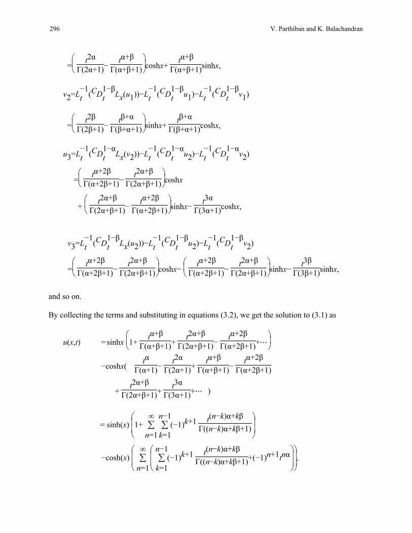
and so on. By collecting the terms and substituting in equations (3.2), we get the solution to (3.1) as

u(x,t) = sinhx

1+ tα+β

Γ(α+β+1)+ t2α+β

Γ(2α+β+1)− tα+2β

Γ(α+2β+1)+⋯

−coshx( tα

Γ(α+1)− t2α

Γ(2α+1)+ tα+β

Γ(α+β+1)− tα+2β

Γ(α+2β+1)

+ t2α+β

Γ(2α+β+1)+ t3α

Γ(3α+1)+⋯ )

= sinh(x)

1+ n=1

∞

k=1

n−1 (−1)k+1

t(n−k)α+kβ

Γ((n−k)α+kβ+1)

−cosh(x)

n=1

∞

k=1

n−1 (−1)k+1

t(n−k)α+kβ

Γ((n−k)α+kβ+1)+(−1)n+1tnα ,


v(x,t) =coshx

1+ tα+β

Γ(α+β+1)− t2α+β

Γ(2α+β+1)+ tα+2β

Γ(α+2β+1)+⋯

−sinhx( tβ

Γ(β+1)− t2β

Γ(2β+1)+ tα+β

Γ(α+β+1)+ tα+2β

Γ(α+2β+1)

− t2α+β

Γ(2α+β+1)+ t3β

Γ(3β+1)+⋯ )

=cosh(x)

1+ n=1

∞

k=1

n−1 (−1)k+1

t(n−k)β+kα

Γ((n−k)β+kα+1)

−sinh(x)

n=1

∞

k=1

n−1 (−1)k+1

t(n−k)β+kα

Γ((n−k)β+kα+1)+(−1)n+1tnβ .

Table 1. Numerical results showing u(x,t) and v(x,t) for different values of α and β by arbitrarily fixing x=3 and t=0.1 using Adomian Decomposition Method and Homotopy Analysis Method (2009)

ADM HAM (2009) α β u(x,t) v(x,t) u(x,t) v(x,t) 0.2 5.82663 5.96672 5.82663 5.96672 0.4 5.83636 6.85362 5.82663 6.84975

0.2 0.6 5.84475 7.74879 5.82663 7.74517 0.8 5.85115 8.52987 5.82663 8.52726 1.0 5.85546 9.11625 5.82663 9.11458 0.2 6.76122 5.95700 6.76509 5.96672 0.4 6.76509 6.84975 6.76509 6.84975

0.4 0.6 6.76834 7.74680 6.76509 7.74517 0.8 6.77076 8.52876 6.76509 8.52726 1.0 6.77235 9.11562 6.76509 9.11458 0.2 7.67438 5.94860 7.67799 5.96672 0.4 7.67636 6.84649 7.67799 6.84975

0.6 0.6 7.67799 7.74517 7.67799 7.74517 0.8 7.67917 8.52788 7.67799 8.52726 1.0 7.67992 9.11513 7.67799 9.11458 0.2 8.46545 5.94221 8.46805 5.96672 0.4 8.46655 6.84408 8.46805 6.84975

0.8 0.6 8.46743 7.7440 8.46805 7.74517 0.8 8.46805 8.52726 8.46805 8.52726 1.0 8.46844 9.11479 8.46805 9.11458 0.2 9.0579 5.9379 9.05956 5.96672 0.4 9.05853 6.84248 9.05956 6.84975

1.0 0.6 9.05902 7.74324 9.05956 7.74517 0.8 9.05935 8.52687 9.05956 8.52726 1.0 9.05956 9.11458 9.05956 9.11458


The solution obtained above in series form is convergent for all values of 0<α,β<1. The convergence of the series can be easily examined by using the ratio test. Table 1 shows the numerical results obtained from Adomian decomposition method and homotopy analysis method [Jafari et al. (2009)]. From the table, one can observe that there is no effect of β on u(x,t) and α on v(x,t) while using HAM obtained in [Jafari et al. (2009)], which is not accurate since the problem considered is coupled. This difficulty is overcome when we use the ADM. The exactness of the solution is clear by its convergence to the exact solution when

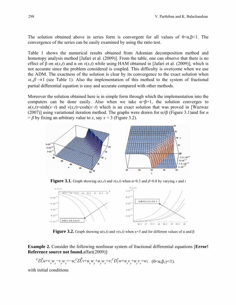
, 1 (see Table 1). Also the implementation of this method to the system of fractional partial differential equation is easy and accurate compared with other methods. Moreover the solution obtained here is in simple form through which the implementation into the computers can be done easily. Also when we take α=β=1, the solution converges to u(x,t)=sinh(x−t) and v(x,t)=cosh(x−t) which is an exact solution that was proved in [Wazwaz (2007)] using variational iteration method. The graphs were drawn for α≠β (Figure 3.1)and for α = β by fixing an arbitrary value to x, say x = 3 (Figure 3.2).

Figure 3.1. Graph showing u(x,t) and v(x,t) when α=0.3 and β=0.8 by varying x and t

Figure 3.2. Graph showing u(x,t) and v(x,t) when x=3 and for different values of α and β

Example 2. Consider the following nonlinear system of fractional differential equations [Error! Reference source not found.affari(2009)]:

CDαt u+v

xw

y−v

yw

x=−u;CD

βt v+u

xw

y+u

yw

x=v;CD

γt w+u

xv

y+u

yv

x=w; (0<α,β,γ<1).

with initial conditions


u(x,y,0)=u0,v(x,y,0)=v

0 and w(x,y,0)=w

0.

By using the properties of Caupto derivative, we can rewrite the given system as

CDtu=CD1−αt (−vxwy+vywx)−CD

1−αt u,

CDtv=CD1−βt (−uxwy−uywx)+CD

1−βt v,

CDtw=CD1−γt (−uxvy−uyvx)+CD

1−γt w.

As we did in the first example let us take CDt(⋅) as Lt(⋅). So L−1t (⋅) may be taken as

0

t (⋅)dt.

Then, the above equation becomes

u = u(x,y,0)+L−1t (CD

1−αt (−vxwy+vywx))−L

−1t (CD

1−αt u),

v = v(x,y,0)+L−1t (CD

1−αt (−uxwy- uywx))−L

−1t (CD

1−αt v),

w = w(x,y,0)+L−1t (CD

1−γt (−uxvy−uyvx))+L

−1t (CD

1−γt w).

If we take the initial conditions as

u0=u(x,y,0),

v0=v(x,y,0),

w0=w(x,y,0),

then, by using the ADM, we get

u1=L

−1t (CD

1−αt (A

0))−L

−1t (CD

1−αt u),

v1=L

−1t (CD

1−βt (B

0))+L

−1t (CD

1−βt v),

w1=L

−1t (CD

1−γt (C

0))+L

−1t (CD

1−γt w),

and, for n>1, we have

un= L

−1t (CD

1−αt (A

n−1))−L

−1t (CD

1−αt u),

vn=L

−1t (CD

1−βt (B

n−1))+L

−1t (CD

1−βt v),

wn=L

−1t (CD

1−γt (C

n−1))+L

−1t (CD

1−γt w),


where An, Bn, and Cn are Adomian polynomials corresponding to the non-linear terms

(−vxwy+vywx), (−uxwy−uywx), and (−uxvy−uyvx) respectively. Then the solution is given by

u= n=0

∞ un,v=

n=0

∞ vn and w=

n=0

∞ wn.

For example, if we take the initial conditions as ex+y, ex−y, e−x+y, then the iterations become

u0=ex+y,

v0=ex−y,

w0=e−x+y,

u1=L−1t (CD

1−αt (A0))−L

−1t (CD

1−αt u0)=−

ex+ytα

Γ(1+α),

v1=L−1t (CD

1−βt (B0))+L

−1t (CD

1−βt v0)=

ex−ytβ

Γ(1+β),

w1=L−1t (CD

1−γt (C0))+L

−1t (CD

1−γt w0)=

e−x+ytγ

Γ(1+γ) ,

u2=L−1t (CD

1−αt (A1))−L

−1t (CD

1−αt u1)=

ex+yt2α

Γ(1+2α),

v2=L−1t (CD

1−βt (B1))+L

−1t (CD

1−βt v1)=

ex−yt2β

Γ(1+2β),

w2=L−1t (CD

1−γt (C1))+L

−1t (CD

1−γt w1)=

ex−yt2γ

Γ(1+2γ),

and so on. By collecting the terms, we get the solution as

u(x,y,t) =ex+y

1+ m=1

∞

(−tα)m

Γ(mα+1) =ex+yEα(−tα),

v(x,y,t) =ex−y

1+ m=1

∞

(tβ)m

Γ(mβ+1) =ex−yEβ(tβ),

w(x,y,t) =e−x+y

1+ m=1

∞

(tγ)m

Γ(mγ+1) =e−x+yEγ(tγ).


The series solution converges to the Mittag-Leffler function of the first kind which is the exact solution of the problem that can be verified by directly substituting into the equation. Also, when we substitute α = β = γ = 1, the solution converges to

u(x,y,t)=ex+y−t, v(x,y,t)=ex−y+t, w(x,y,t)=e−x+y+t,

which was proved by Wazwaz(2007) for integer type problem using variational iteration method. Also the same results are obtained in [Jafari et al. (2009)] using homotopy analysis method. The graphs (Figures 3.3 - 3.5) are plotted for different values of α,β and γ by fixing arbitrary values of x and y, say x=0.5 and y=0.5.

Figure 3.3. Graph showing u(x,y,t) , when x=y=0.5 and for different values of α, β and γ

Figure 3.4. Graph showing v(x,y,t) when x=y=0.5 and for different values of α, β and γ

Figure 3.5. Graph showing w(x,y,t) when x=y=0.5 and for different of α, β and γ


4. Conclusion In this paper, Adomain decomposition method is efficiently used to obtain the solution of the system of fractional partial differential equations. Since its convergence to the exact solution, when the system is of integer order, proves that this method is very much effective to solve the system of partial differential equations. However, the necessity of discretization or perturbation is not needed, the method can be easily implemented using any symbolic mathematical softwares. It is observed that the results obtained in this article can be extended to any system of n fractional partial differential equations. Moreover, it provides more realistic series solutions that converge very rapidly in real physical problems.

Acknowledgement

The authors are thankful to the referees for giving the fruitful suggestions for the improvement of the paper.

REFERENCES

Abassy, T.A. (2010). Improved Adomian decomposition method, Computers and Mathematics

with Applications, 59 (2010), 42 - 54. Adomian, G. (1994). Solving Frontier Problems of Physics, Kluwer, London. Adomian, G. (1996). Solution of coupled nonlinear partial differential equations by

decomposition, Computers and Mathematics with Applicatons, 31, 117 - 120. Barkai, E., Metzler, R. and Klafter, J. (2000). From continuous time random walks to the

fractional fokker-planck equation, Physics Review E, 61, 132-138. Biazar, J., Babolian, E. and Islam, R. (2004). Solution of the system of ordinary differential

equations by Adomian decomposition method, Applied Mathematics and Computation, 147, 713 - 719.

Biazar, J. (2005). Solution of systems of integral - differential equations by Adomian decomposition method, Applied Mathematics and Computation, 168, 1232 - 1238.

Bougoffa, L. and Bougouffa, S. (2006). Adomian method for solving some coupled systems of two equations, Applied Mathematics and Computation, 177 (2006), 553 - 560.

Caponetto, R., Dongola, G., Fortuna, L. and Petrás, I. (2010). Fractional Order Systems: Modeling and Control Applications, World Scientific Publishing Company, Singapore.

Daftardar-Gejji, V. and Bhalekar, S. (2008). Solving multi-term linear and non-linear diffusion wave equations of fractional order by Adomian decomposition method, Applied Mathematics and Computation, 202, 113 - 120.

Daftardar-Gejji, V. and Jafari, H. (2007). Solving a multi-order fractional differential equation using adomian decomposition, Applied Mathematics and Computation, 189, 541 - 548.

Diethelm, K. (2010). The Analysis of Fractional Differential Equations, Springer, New York. El-Sayed, A.M.A., Behiry, S.H. and Raslan, W.E. (2010). Adomian’s decomposition method for

solving an intermediate fractional advection -dispersion equation, Computers and Mathematics with Applications, 59, 1759 - 1765.


Evans, D.J. and Raslan, K.R. (2005). The Adomian decomposition method for solving delay differential equation, International Journal of Computer Mathematics, 82, 49 - 54.

Fakharian, A., Hamidi Beheshti, M.T. and Davari, A. (2010). Solving the Hamiltonâ€“Jacobiâ€“Bellman equation using Adomian decomposition method, International Journal of Computer Mathematics, 87, 2769 - 2785.

Gu, H. and Li, Z. (2007). A modified Adomian method for system of nonlinear differential equations, Applied Mathematics and Computation, 187, 748 - 755.

Hernández, E., O’Regan, D. and Balachandran, K. (2010). On recent developments in the theory of abstract differential equations with fractional derivatives, Nonlinear Analysis: Theory, Methods and Applications, 73, 3462 - 3471.

Hosseini, M.M. and Jafari, M. (2009). A note on the use of Adomian decomposition method for high-order and system of nonlinear differential equations. Communication in Nonlinear Science and Numerical Simulation, 14, 1952 - 1957.

Hosseini, M.M. and Nasabzadeh, H. (2006). On the convergence of Adomian decomposition method, Applied Mathematics and Computation, 182, 536 - 543.

Hu, Y., Luo, Y. and Lu, Z. (2008). Analytical solution of the linear fractional differential equation by Adomian decomposition method, Journal of Computational and Applied Mathematics, 215, 220 - 229.

Jafari, H. and Seifi, S. (2009). Solving a system of nonlinear fractional partial differential equations using homotopy analysis method, Communication in Nonlinear Science and Numerical Simulation, 14, 1962 - 1969.

Javadi, S., Davari, A. and Babolian, E. (2007). Numerical implementation of the Adomian decomposition method for nonlinear Volterra integral equations of the second kind, International Journal of Computer Mathematics, 84, 75 - 79.

Junsheng, D., Jianye, A. and Mingyu, X. (2007). Solution of system of fractional differential equations by Adomian decompositon method, Applied Mathematics - A Journal of Chinese Universities. Series B, 22, 7 - 12.

Kilbas, A.A., Srivastava, H.M. and Trujillo, J.J. (2006). Theory and Applications of Fractional Differential Equations, Elsevier, Amstrdam.

Li, C. and Wang, Y. (2009). Numerical algorithm based on Adomian decomposition for fractional differential equations, Computers and Mathematics with Applications, 57, 1672 - 1681.

Luchko, Yu. and Gorenflo, R. (1999). An operational method for solving fractional differential equations with the Caputo derivatives, Acta Mathematica Vietnamica, 24, 207-233.

Machado, J. T., Kiryakova, V. and Mainardi, F. (2010). Recent history of fractional calculus, Communication in Nonlinear Science and Numerical Simulation, 16, 1140-1153.

Machado, J.T., Luo, A.C.J., Barbosa, R.S., Silva, M.F. and L.B. Figueiredo, (2011). Nonlinear Science and Complexity, Springer, New York.

Magin, R., Ortigueira, M.D., Podlubny, I. and Trujillo, J.J. (2011). On the fractional signals and systems, Signal Processing, 91, 350-371.

Mainardi, F. (2010). Fractional Calculus and Waves in Linear Viscoelasticity: An Introduction to Mathematical Models, Imperial College Press, London.

Mamchuev, M. O. (2008). Boundary value problem for a system of fractional partial differential equations, Differential Equations, 44, 1737 - 1749.

Meerschaert, M. M., Benson, D. A., Scheffler, H. P. and Becker-Kern, P. (2002). Governing equations and solutions of anomalous random walk limits, Physics Review E, 66, 102-105.


Miller, K. and Ross, B. (1993). An Introduction to the Fractional Calculus and Fractional Differential Equations, Wiley and Sons, New York.

Oldham, K.B. and Spanier, J. (1974). The Fractional Calculus: Theory and Application of Differention and Integration to Arbitrary order, Academic Press, California.

Podlubny, I. (1999). Fractional Differential Equations, Academic Press, California. Saha Ray, S. (2009). Analytical solution for the space fractional diffusion equation by two-step

Adomian Decomposition Method, Communications in Nonlinear Science and Numerical Simulation, 14, 1295 - 130.

Samko, S.G., Kilbas, A.A. and Marichev, O.I. (1993). Fractional Integrals and Derivatives; Theory and Applications,Gordan and Breach, Amsterdam.

Tadjeran, C. and Meerschaert, M.M. (2007). A second order accurate numerical method for the two-dimensional fractional diffusion equation, Journal of Computational Physics, 220, 813 - 823.

Wang, Q. (2006). Numerical solutions for fractional KdV-Burgers equation by Adomian decomposition method, Applied Mathematics and Computation, 182, 1048 - 1055.

Wazwaz, A.M. (2007). The variational iteration method for solving linear and nonlinear systems of PDEs, Computers and Mathematics with Applications, 54, 895 - 902.

solutions of system of fractional partial differential ......solvability of a boundary value problem...

Documents