solutions manual for recursive methods in economic dynamics · pdf filesolutions manual for...
TRANSCRIPT

Solutions Manual for
Recursive Methodsin Economic Dynamics


Solutions Manual for
Recursive Methodsin Economic Dynamics
Claudio Irigoyen
Esteban Rossi-Hansberg
Mark L. J. Wright
Harvard University PressCambridge, Massachusetts, and London, England2002

Copyright c° 2002 by the President and Fellows of Harvard CollegeAll rights reservedPrinted in the United States of America
Library of Congress Cataloging-in-Publication Data

To Marta, Santiago, and Federico— CI
To Maria Jose— ERH
To Christine— MLJW

Contents
1 Introduction 1
2 An Overview 3
3 Mathematical Preliminaries 20
4 Dynamic Programming under Certainty 43
5 Applications of Dynamic Programming under Certainty 56
6 Deterministic Dynamics 85
7 Measure Theory and Integration 102
8 Markov Processes 137
9 Stochastic Dynamic Programming 154
10 Applications of Stochastic Dynamic Programming 179
11 Strong Convergence of Markov Processes 199
12 Weak Convergence of Markov Processes 208
13 Applications of Convergence Results for Markov Processes 223
14 Laws of Large Numbers 246
15 Pareto Optima and Competitive Equilibria 252
vi

vii
16 Applications of Equilibrium Theory 266
17 Fixed-Point Arguments 284
18 Equilibria in Systems with Distortions 298
Foreword
Over the years we have received many requests for an answer bookfor the exercises in Recursive Methods in Economic Dynamics. Theserequests have come not from inept teachers or lazy students, but fromserious readers who have wanted to make sure their time was beingwell spent.
For a student trying to master the material in Recursive Methods,the exercises are critical, and some of them are quite hard. Thus it isuseful for the reader to be reassured along the way that he or she is onthe right track, and to have misconceptions corrected quickly whenthey occur. In addition, some of the problems need more specificguidelines or sharper formulations, and a few (not too many, we liketo think) contain errors — commands to prove assertions that, underthe stated assumptions, are just not true.
Consequently, when three of our best graduate students proposedto write a Solutions Manual, we were delighted. While we firmlybelieve in the value of working out problems for oneself, in learningby doing, it is clear that the present book will be an invaluable aidfor students engaged in this enterprise.
The exercises in Recursive Methods are of two types, reflectingthe organization of the book. Some chapters in the book are self-contained expositions of theoretical tools that are essential to mod-ern practitioners of dynamic stochastic economics. These “core”chapters contain dozens of problems that are basically mathemat-ical: exercises to help a reader make sure that an abstract definitionor theorem has been grasped, or to provide a proof (some of themquite important) that was omitted from the text. This SolutionsManual contains solutions for most of the exercises of this sort. In
viii

ix
particular, proofs are provided for results that are fundamental inthe subsequent development of the theory.
Other chapters of Recursive Methods contain applications of thosetheoretical tools, organized by the kind of mathematics they require.The exercises in these chapters are quite different in character. Manyof them guide the reader through classic papers drawn from varioussubstantive areas of economics: growth, macroeconomics, monetarytheory, labor, information economics, and so on. These papers, whichappeared in leading journals over the last couple of decades, repre-sented the cutting edge, both technically and substantively. Turninga paper of this sort into an exercise meant providing enough struc-ture to keep the reader on course, while leaving enough undone tochallenge even the best students. The present book provides answersfor only a modest proportion of these problems. (Of course, for manyof the rest the journal article on which the problem is based providesa solution!)
We hope that readers will think of this Solutions Manual as atrio of especially helpful classmates. Claudio, Esteban, and Markare people you might look for in the library when you are stuck ona problem and need some help, or with whom you want to comparenotes when you have hit on an especially clever argument. This isthe way a generation of University of Chicago students have thoughtof them, and we hope that this book will let many more students, ina wide variety of places, benefit from their company as well.
Nancy L. Stokey
Robert E. Lucas

Solutions Manual for
Recursive Methodsin Economic Dynamics

1 Introduction
In the preface to Recursive Methods in Economic Dynamics, the au-thors stated that their aim was to make recursive methods accessibleto the wider economics profession. They succeeded. In the decadesince RMED appeared, the use of recursive methods in economicshas boomed. And what was once as much a research monographas a textbook has now been adopted in first-year graduate coursesaround the world.
The best way for students to learn these techniques is to workproblems. And towards this end, RMED contains over two hundredproblems, many with multiple parts. The present book aims to assiststudents in this process by providing answers and hints to a largesubset of these questions.
At an early stage, we were urged to leave some of the questionsin the book unanswered, so as to be available as a “test bank” forinstructors. This raises the question of which answers to includeand which to leave out. As a guiding principle, we have tried toinclude answers to those questions that are the most instructive, inthe sense that the techniques involved in their solution are the mostuseful later on in the book. We have also tried to answer all of thequestions whose results are integral to the presentation of the coremethods of the book. Exercises that involve particularly difficultreasoning or mathematics have also been solved, although no doubtour specific choices in this regard are subject to criticism.
As a result, the reader will find that we have provided an answerto almost every question in the core “method” chapters (that is,Chapters 4, 6, 9, 15, 17, and 18), as well as to most of the questionsin the chapters on mathematical background (Chapters 3, 7, 8, 11,
1

2 1 / Introduction
12, and 14). However, only a subset of the questions in “application”chapters (2, 5, 10, 13, and 16) have been answered.
It is our hope that this selection will make the assimilation of thematerial easier for students. At the same time, instructors should becomforted to find that they still have a relatively rich set of questionsto assign from the applications chapters. Instructors should also findthat, because much of the material in the method and mathematicalbackground chapters appears repeatedly, there are many opportuni-ties to assign this material to their students.
Despite our best efforts, errors no doubt remain. Furthermore,it is to be expected (and hoped) that readers will uncover more el-egant, and perhaps more instructive, approaches to answering thequestions than those provided here. The authors would appreciatebeing notified of any errors and, as an aid to readers, commit tomaintaining a website where readers can post corrections, commentsand alternative answers. This website is currently hosted at:
http://home.uchicago.edu/~mwright2/SLPSolutions.html
In the process of completing this project we have incurred vari-ous debts. A number of people provided us with their own solutionsto problems in the text, including Xavier Gine and Rui Zhao. Oth-ers, including Vadym Lepetyuk, Joon Hyuk Song and Ivan Wern-ing, pointed out sins of commission and omission in earlier drafts.Christine Groeger provided extensive comments, and lent her LATEXexpertise to the production of the manuscript. We thank all of thesepeople, and reserve a special thanks for Nancy Stokey, whose insightand enthusiasm were invaluable in seeing the project through to itsconclusion.

2 An Overview
Exercise 2.1
The fact that f : R+ → R+ is continuously differentiable, strictlyincreasing and strictly concave comes directly from the definition off as
f(k) = F (k, 1) + (1− δ)k,
with 0 < δ < 1, and F satisfying the properties mentioned above.In particular, the sum of two strictly increasing functions is strictlyincreasing, and continuous differentiability is preserved under sum-mation. Finally, the sum of a strictly concave and a linear functionis strictly concave.
Also,
f(0) = F (0, 1) = 0,
f 0(k) = Fk(k, 1) + (1− δ) > 0,
limk→0
f 0(k) = limk→0
Fk(k, 1) + limk→0
(1− δ) =∞,limk→∞
f 0(k) = limk→∞
Fk(k, 1) + limk→∞
(1− δ) = (1− δ).
Exercise 2.2
a. With the given functional forms for the production andutility function we can write (5) as
αβkα−1t
kαt − kt+1=
1
kαt−1 − kt,
3

4 2 / An Overview
which can be rearranged as
αβkα−1t (kαt−1 − kt) = (kαt − kt+1).
Dividing both sides by kαt and using the change of variable zt =kt/k
αt−1 we obtain
αβ(1
zt− 1) = 1− zt+1,
or
zt+1 = 1 + αβ − αβ
zt,
which is the equation represented in Figure 2.1.
Insert Figure 2.1 About Here
As can be seen in the figure, the first-order difference equationhas two steady states (that is, z’s such that zt+1 = zt = z), whichare the two solutions to the characteristic equation
z2 − (1 + αβ)z + αβ = 0.
These are given by z = 1 and αβ.
b. Using the boundary condition zT+1 = 0 we can solve forzT as
zT =αβ
1 + αβ.
Substituting recursively into (??) we can solve for zT−1 as
zT−1 =αβ
1 + αβ − zT=
αβ
1 + αβ − αβ1+αβ
=αβ(1 + αβ)
1 + αβ + (αβ)2,

2 / An Overview 5
and in general,
zT−j =αβ[1 + αβ + ...+ (αβ)j ]
1 + αβ + ...+ (αβ)j+1.
Hence for t = T − j,
zt =αβ[1 + αβ + ...+ (αβ)T−t]1 + αβ + ...+ (αβ)T−t+1
=αβsT−tsT−t+1
where si = 1+ αβ + ...+ (αβ)i. In order to solve for the series, takefor instance the one in the numerator,
sT−t = 1 + αβ + ...+ (αβ)T−t,
multiply both sides by αβ to get
αβsT−t = αβ + ...+ (αβ)T−t+1,
and substract this new expression from the previous one to obtain
(1− αβ)sT−t = 1− (αβ)T−t+1.
Hence
sT−t =1− (αβ)T−t+1
1− αβ,
sT−t+1 =1− (αβ)T−t+2
1− αβ,
and therefore
zt = αβ1− (αβ)T−t+11− (αβ)T−t+2 ,
for t = 1, 2, ..., T + 1, as in the text. Notice also that
zT+1 = αβ1− (αβ)T−(T+1)+11− (αβ)T−(T+1)+2
= 0.

6 2 / An Overview
c. Plugging (7) into the right hand side of (5) we getkαt−1 − αβ
h1− (αβ)T−t+1
ih1− (αβ)T−t+2
ikαt−1−1 =
h1− (αβ)T−t+2
ikαt−1 (1− αβ)
.
Similarly, by plugging (7) into the left hand side of (5) we obtain
αβ
·αβ[1−(αβ)T−t+1][1−(αβ)T−t+2]k
αt−1
¸α−1·αβ[1−(αβ)T−t+1][1−(αβ)T−t+2]k
αt−1
¸αµ1− αβ
[1−(αβ)T−t][1−(αβ)T−t+1]
=1
kαt−1
h1− (αβ)T−t+1
i− αβ
h1− (αβ)T−t
ih1− (αβ)T−t+2
i−1
=
h1− (αβ)T−t+2
ikαt−1 (1− αβ)
.
Hence, the law of motion for capital given by (7) satisfies (5).Evaluating (7) for t = T yields
kT+1 = αβ1− (αβ)T−T1− (αβ)T−T+1k
αT
= 0,
so (7) satisfies (6) too.
Exercise 2.3
a. We can write the value function using the optimal pathfor capital given by (8) as
υ(k0) =∞Xt=0
βt log(kαt − αβkαt )
=log(1− αβ)
(1− β)+ α
∞Xt=0
βt log(kt).

2 / An Overview 7
The optimal policy function, written (by recursive substitution) as afunction of the initial capital stock is (in logs)
log kt =
Ãt−1Xi=0
αi
!log(αβ) + αt log k0.
Using the optimal policy function we can break up the last summa-tion to get
∞Xt=0
βt log(kt) =log(k0)
(1− αβ)+ log(αβ)
∞Xt=1
βtµt−1Pi=0
αi
=log(k0)
(1− αβ)+ β
log(αβ)
[(1− β)(1− αβ)],
where we have used the fact that the solution to a series of theform st =
Pti=0 λ
i is¡1− λt+1
¢/ (1− λ) , as shown in Exercise 2.2b.
Hence, we obtain a log linear expression for the value function
υ(k0) = A+B log(k0),
where
A =
·log(1− αβ) +
αβ log(αβ)
(1− αβ)
¸(1− β)−1,
and
B =α
1− αβ.
b. We want to verify that
υ(k) = A+B log(k)
satisfies (11). For this functional form, the first-order condition ofthe maximization problem in the right-hand side of (11) is given by
g(k) =βB
1 + βBkα.

8 2 / An Overview
Plugging this policy function into the right hand side of (11) weobtain
υ(k) = log
µkα − βB
1 + βBkα¶+ β
·A+B log
µβB
1 + βBkα¶¸
= α log (k)− log (1 + βB) + βA
+βB [log (βB) + α log (k)− log (1 + βB)]
= (1 + βB)α log (k)− (1 + βB) log(1 + βB)
+βA+ βB log(βB).
Using the expressions for A and B obtained in part a., we get that(1 + βB)α = B and
βB log(βB)− (1 + βB) log(1 + βB) + βA = A,
and hence υ(k) = A+B log (k) satisfies (11) .
Exercise 2.4
a. The graph of g(k) = sf(k), with 0 < s < 1, is found inFigure 2.2.
Insert Figure 2.2 About Here.
Since f is strictly concave and continuously differentiable, g willinherit those properties. Also, g(0) = sf(0) = 0. In addition,
limk→0
g0(k) = limk→0
sf 0(k)
= limk→0
sFk(k, 1) + limk→0
s(1− δ) =∞,
and
limk→∞
g0(k) = limk→∞
sf 0(k)
= limk→∞
sFk(k, 1) + limk→∞
s(1− δ) = s(1− δ) < 1.

2 / An Overview 9
First, we will prove existence of a non-zero stationary point.Combining the first limit condition (the one for k → 0) and
g(0) = 0, we have that for an arbitrary small positive perturbation,
0 <g(0 + h)− g(0)
h.
This term tends to +∞ as h→ 0, and hence g(h)/h→∞. Therefore,there exist an h such that g(h)/h > 1, and hence g(k) > k for somek small enough. Similarly, the fact that g(k) < k for k large enoughis a direct implication of the second limit condition. Next, defineq(k) = g(k) − k. By the arguments outlined above, q(k) > 0 for ksmall enough and q(k) < 0 for k large enough. By continuity of f,q is also continuous and hence by the Intermediate Value Theoremthere exist a k∗ such that g(k∗) = k∗.
That the stationary point is unique follows from the strict con-cavity of g. Note that a continuum of stationary points implies thatg0(k) = 1 contradicting the strict concavity of g. A discrete set of sta-tionary points will imply that one of the stationary points is reachedfrom below, violating again the strict concavity of g. To see this, de-fine k∗ = min k ∈ R+ : q(k) = 0. The limit conditions above, andthe fact that g is nondecreasing implies that g(k∗−ε) > k∗, for ε > 0.Define
km = min k ∈ R+ : q(k) = 0, k > k∗ and g(k − ε)− k > 0 for ε > 0 .
Then, by continuity of g, there exist k ∈ (k∗, km) such that g(k) <k. Let α ∈ (0, 1) be such that k = αk∗ + (1− α)km. Then,
αg(k∗) + (1− α)g(km) = αk∗ + (1− α)km
= k
> g(k)
= g(αk∗ + (1− α)km),
a contradiction.
b. In Figure 2.3, we can see how for any k0 > 0, the se-quence kt∞t=0 converges to k∗ as t → ∞. As can be seen too, this

10 2 / An Overview
convergence is monotonic, and it does not occur in a finite numberof periods if k0 6= k∗.
Insert Figure 2.3 About Here
Exercise 2.5
Some notation is needed. Let zt denote the history of shocksup to time t. Equivalently, zt = (zt−1, zt), where zt is the shock inperiod t.
Consumption and capital are indexed by the history of shocks.They are chosen given the information available at the time the de-cision is taken, so we represent them by finite sequences of randomvariables c =
©ct(z
t)ªTt=0
and k =©kt(z
t)ªTt=0.
The pair (kt, zt) determines the set of feasible pairs (ct, kt+1) ofcurrent consumption and beginning of next period capital stock. Wecan define this set as
B(kt, zt) =
©(ct, kt+1) ∈ R2+ : ct(zt) + kt+1(zt) ≤ ztf [kt(zt−1)]
ªBecause the budget constraint should be satisfied for each t and
for every possible state, Lagrange multipliers are also random vari-ables at the time the decisions are taken, and they should also beindexed by the history of shocks, so λt(zt−1, zt) is a random variablerepresenting the Lagrange multiplier for the time t constraint.
The objective function
U(c0, c1, ...) = E
( ∞Xt=0
βtu[ct(zt)]
)can be written as a nested sequence,
u(c0) + βnXi=1
πi
u[c1(ai)] + βnXj=1
πj [u(c2(ai, aj) + β [...]]
,where πi stands for the probability that state ai occurs.

2 / An Overview 11
The objects of choice are then the contingent sequences c and k.For instance
c =©c0, c1(z
1), c2(z2), .., ct(z
t), ..cT (zT )ª.
We can see that c0 ∈ R+, c1 ∈ Rn+, c2 ∈ R2n+ , and so on, so thesequence c belongs to the obvious cross product of the commodityspaces for each time period t. Similar analysis can be carried out forthe capital sequence
k =©k0, k1(z
1), k2(z2), .., kt(z
t), ..kT (zT )ª.
Define this cross product as S. Hence we can define the consumptionset as
C(k0, z0) =©c ∈ S : £ct(zt), kt+1(zt)¤ ∈ B(kt, zt),t = 0, 1, ... for some k ∈ S, k0 given.
(Notice that the consumption set, i.e. the set of feasible sequences,is a subset of the Euclidean space defined above.)
The first order conditions for consumption and capital are, re-spectively, (after cancelling out probabilities on both sides):
u0[ct(zt, zt−1)] = λt(zt, zt−1)
for all¡zt−1, zt
¢and all t, and
λt(zt, zt−1) =
nXi=1
πiλt(ai, ztj)f
0[kt(ai, zt−1)]
for all¡zt−1, zt
¢and all t.
Exercise 2.6
As we did before in the deterministic case, we can use the budgetconstraint to solve for consumption along the optimal path and then

12 2 / An Overview
write the value function as
υ(k0, z0) = E0
" ∞Xt=0
βt log(ztkαt − αβztk
αt )
#
=log(1− αβ)
(1− β)+E0
" ∞Xt=0
βt log(zt)
#
+αE0
" ∞Xt=0
βt log(kt)
#.
To obtain an expression in terms of the initial capital stock and theinitial shock we need to solve for the second and third term above.Denoting E0(log zt) = µ, the second term can be written as
E0
" ∞Xt=0
βt log(zt)
#= log z0 +
∞Xt=0
βtE0(log zt)
= log z0 +βµ
1− β.
In order to solve for the third term, we use the fact that the optimalpath for the log of the capital stock can be written as
log kt =
Ãt−1Xi=0
αi
!log(αβ) +
Ãt−1Xi=0
αt−1−i!log(zi) + αt log k0.
Hence
αE0
" ∞Xt=0
βt log(kt)
#= αE0
" ∞Xt=1
βt
Ãt−1Xi=0
αi
!log(αβ)
#
+αE0
" ∞Xt=1
βtµt−1Pi=0
αt−1−i log(zi)¶#
+αE0
" ∞Xt=1
(αβ)t log(k0)
#+ α log k0.
Therefore, the next step is to solve for each of the terms above. The

2 / An Overview 13
first term can be written as
αE0
" ∞Xt=1
βtµt−1Pi=0
αi¶log(αβ)
#= α log(αβ)
∞Xt=1
βtµ1− αt
1− α
¶=
α log(αβ)
(1− α)
·β
(1− β)− αβ
(1− αβ)
¸=
αβ log(αβ)
(1− β)(1− αβ),
the second term as
αE0
" ∞Xt=1
βt
Ãt−1Xi=0
αt−1−i log(zi)
!#
= αE0
"β log(z0) +
∞Xt=2
βt
Ãt−1Xi=0
αt−1−i log(zi)
!#
= αE0
"β log(z0) +
∞Xt=2
βt
Ãαt−1 log(z0) +
t−1Xi=1
αt−1−i log(zi)
!#
=αβ log(z0)
(1− αβ)+ α
∞Xt=2
βt
Ãt−1Xi=1
αt−1−iµ
!
=αβ log(z0)
(1− αβ)+
αµ
(1− α)
∞Xt=2
βt(1− αt−1)
=αβ log(z0)
(1− αβ)+
αβ2µ
(1− β)(1− αβ),
and finally, the last two terms as
αE0
" ∞Xt=1
(αβ)t log(k0)
#+ α log k0 =
α log k0(1− αβ)
.
Hence,
αE0
" ∞Xt=0
βt log(kt)
#=
αβ log(αβ)
(1− β)(1− αβ)+
αβ log(z0)
(1− αβ)
+αβ2µ
(1− β)(1− αβ)+
α log k0(1− αβ)
,

14 2 / An Overview
andυ(k0, z0) = A+B log(k0) + C log(z0)
where
A =
·log(1− αβ) +
αβ log(αβ)
(1− αβ)+
βµ
(1− αβ)
¸(1− β)−1,
B =α
(1− αβ), and
C =1
(1− αβ).
Following the same procedure outlined in Exercise 2.3, it can bechecked that υ satisfies (3) .
Exercise 2.7
a. The sequence of means and variances of the sequence oflogs of the capital stocks have a recursive structure. Define µt as themean at time zero of the log of the capital stock in period t. Then
µt = E0[log kt]
= E0[log(αβ) + α log(kt−1) + log(zt−1)]= log(αβ) + µ+ αµt−1= log(αβ) + µ+ α [log(αβ) + µ] + α2µt−2= [log(αβ) + µ] +
£1 + α+ ...+ αt−1
¤+ αtµ0
=
·µ0 −
log(αβ) + µ
1− α
¸αt +
log(αβ) + µ
1− α.
Since 0 < α < 1,
µ∞ ≡ limt→∞µt =
log(αβ) + µ
1− α.
Similarly, define σt as the variance at time zero of the log of thecapital stock in period t. Then
σt = V ar0[log kt]
= V ar0[log(αβ) + α log(kt−1) + log(zt−1)]= α2σt−1 + σ,

2 / An Overview 15
which is also an ordinary differential equation with solution given by
σt =
·σ0 − σ
1− α2
¸α2t +
σ
1− α2.
Hence, since 0 < α < 1,
σ∞ ≡ limt→∞σt =
σ
1− α2.
Exercise 2.8
First, we will show that©c∗t , k∗t+1
ªTt=0, k∗T+1 = 0 satisfies the con-
sumer’s intertemporal budget constraint. By (19) and the definitionof f ,
f(k∗t ) = F (k∗t , 1) + (1− δ)k∗t .
Since F is homogeneous of degree one, using (20)−(22) we have that
f(k∗t ) = (r∗t + 1− δ)k∗t + w
∗t = c
∗t + k
∗t+1,
and hence the present value budget constraint (12) is satisfied for theproposed allocation when prices are given by (20)− (22).
The feasibility constraint (16) is satisfied by construction. Hence,in equilibrium, the first order conditions for the representative house-hold are (for ket+1 > 0)
βtU 0[f(ket )− ket+1] = λpt,
λ[(rt+1 + 1− δ)pt − pt] = 0,
f(ket )− cet − ket+1 = 0,
for t = 0, 1, ..., T. Combining them and using (20)− (22) we obtain
U 0£f (ket )− ket+1
¤= βU 0
£f¡ket+1
¢− ket+2¤ f 0(ket ),f(ket )− cet − ket+1 = 0,
for t = 0, 1, ..., T , which by construction is satisfied by the proposedsequence k∗t+1Tt=0. Hence (c∗t , k∗t+1)Tt=0, with k∗T+1 = 0 and k∗0 =x0 solves the consumer’s problem.

16 2 / An Overview
Finally, we need to show that k∗t , n∗t = 1Tt=0 is a maximizingallocation for the firm. Replacing (21) and (22) in (9) and (10)together with the definition of f(k) and the assumed homogeneityof degree 1 of F, we verify that the proposed sequence of prices andallocations satisfy indeed the first-order conditions of the firm, andthat π = 0.
Exercise 2.9
Under the new setup, the household’s decision problem is
max(ct,nt)Tt=0
TXt=0
βtU(ct)
subject toTXt=0
ptct ≤TXt=0
ptwtnt + π;
and0 ≤ nt ≤ 1, ct ≥ 0, t = 0, 1, ..., T.
Similarly, the firm’s problem is
max(kt,it,nt)Tt=0
π = p0(x0 − k0) +TXt=0
pt[yt − wtnt − it]
subject to
it = kt+1 − (1− δ)kt, t = 0, 1, ..., T ;
yt ≤ F (kt, nt), t = 0, 1, ..., T ;
kt ≥ 0, t = 0, 1, ..., T ;
k0 ≤ x0, x0 given.
Hence, x0 can be interpreted as the initial stock of capital and k0 thestock of capital that is effectively put into production, while kt fort ≥ 1 is the capital stock that is chosen one period in advance to bethe effective capital allocated into production in period t.

2 / An Overview 17
As stated in the text, labor is inelastically supplied by house-holds, prices are strictly positive, and the nonnegativity constraintsfor consumption are never binding, so equation (14) in the text isthe first-order condition for the household.
The first-order conditions for the firm’s problem are (after sub-stituting both constraints into the objective function)
wt − Fn(kt, nt) = 0,
−pt + pt+1[Fk(kt, nt) + (1− δ)] ≤ 0,
for t = 0, 1, ..., T, where the latter holds with equality if kt+1 > 0.Evaluating the objective function of the firm’s problem using the
optimal path for capital and labor, we find that first order conditionsare satisfied, and π = p0x0 so the profits of the firm are given by thevalue of the initial capital stock.
Next, it rest to verify that the quantities given by (17) − (19)and the prices defined by (20) − (22) constitute a competitive equi-librium. The procedure is exactly as in Exercise 2.8. In equilibrium,combining the first-order conditions for periods t and t + 1 in thehousehold’s problem we obtain
U 0[f(kt)− kt+1] = βU 0[f(kt+1)− kt+2]f 0(kt+1),f(kt)− ct − kt+1 = 0,
for t = 1, 2, ...T , as before. Hence the proposed sequences constitutesa competitive equilibrium.
Exercise 2.10
The firm’s decision problem remains as stated in (8) (that is, as aseries of one-period maximization problems). Let st be the quantityof one period bonds held by the representative household. Its decisionproblem now is
max(ct,kt+1,st+1,nt)Tt=0
TXt=0
βtU(ct)

18 2 / An Overview
subject to
ct + qtst+1 + kt+1 ≤ rtkk + (1− δ)kt + wtnt, t = 0, 1, ..., T ;
0 ≤ nt ≤ 1, ct ≥ 0, t = 0, 1, ..., T ;
and k0 given.We assume, as in the text, that the whole stock of capital is
supplied to the market. Now, instead of having one present valuebudget constraint, we have a sequence of budget constraint, one foreach period, and we will denote by βtλt the corresponding Lagrangemultipliers.
In addition, we need to add an additional market clearing con-dition for the bond market that must be satisfied in the competitiveequilibrium. This says that bonds are in zero net supply at the statedprices.
Hence, the first-order conditions that characterize the house-hold’s problem are
U 0(ct)− λt = 0,
−λtqt + βλt+1 = 0,
−λt + βλt+1[rt+1 + 1− δ] ≤ 0,
with equality for kt+1 ≥ 0,
and the budget constraints, for t = 0, 1, ..., T.We show next that the proposed allocations (c∗t , k∗t+1)Tt=0 to-
gether with the sequence of prices given by (21) − (22) and thepricing equation for the bond, constitute a competitive equilibrium.Combining the first and second equations evaluated at the proposedallocation, we obtain the pricing equation
qt = βU 0(c∗t+1)U 0(c∗t )
.
>From the first-order conditions of the firm’s problem, and afterimposing the equilibrium conditions, rt = Fk(k∗t , 1)., Combining thefirst-order conditions for consumption and capital for the household’sproblem, we obtain
f 0(k∗t+1)−1 = β
U 0(c∗t+1)U 0(c∗t )
.

2 / An Overview 19
The rest is analogous to the procedure followed in Exercise 2.9.Hence, the sequence of quantities defined by (17) − (19), and theprices defined by (21)− (22) plus the bond price defined in the textindeed define a competitive equilibrium.

3 Mathematical Preliminaries
Exercise 3.1
Given k0 = k, the lifetime utility given by the sequence kt∞t=1in which kt+1 = g0(kt) is
w0(k) =∞Xt=0
βtu[f(kt)− g0(kt)]
= u[f(k)− g0(k)] + β∞Xt=1
βt−1u[f(kt)− g0(kt)].
But
∞Xt=1
βt−1u[f(kt)− g0(kt)] =∞Xt=0
βtu[f(kt+1)− g0(kt+1)]
= w0(k1)
= w0[g0(k)].
Hencew0(k) = u[f(k)− g0(k)] + βw0[g0(k)]
for all k ≥ 0.
Exercise 3.2
a. The idea of the proof is to show that any finite dimensionalEuclidean spaceRl satisfies the definition of a real vector space, usingthe fact that the real numbers form a field.
20

3 / Mathematical Preliminaries 21
Take any three arbitrary vectors x = (x1, ..., xl) , y = (y1, ..., yl)and z = (z1, ..., zl) in Rl. and any two real numbers α and β ∈ R.Define a zero vector θ = (0, ..., 0) ∈ Rl.
Define the addition of two vectors as the element by element sum,and a scalar multiplication by the multiplication of each elementof the vector by a scalar. That any finite Rl space satisfies thoseproperties is trivial.
a :
x+ y = (x1 + y1, x2 + y2, ..., xl + yl)
= (y1 + x1, y2 + x2, ..., yl + xl) = y + x ∈ Rl.
b :
(x+ y) + z = (x1 + y1, ..., xl + yl) + (z1, ..., zl)
= (x1 + y1 + z1, ..., xl + yl + zl)
= (x1, ..., xl) + (y1 + z1, ..., yl + zl)
= x+ (y + z) ∈ Rl.
c :
α(x+ y) = α(x1 + y1, ..., xl + yl)
= (αx1 + αy1, ...,αxl + αyl)
= (αx1, ...,αxl) + (αy1, ...,αyl) = αx+ αy ∈ Rl.
d :
(α+ β)x = ((α+ β)x1, ...(α+ β)xl)
= (αx1 + βx1, ...,αxl + βxl)
= αx+ βx ∈ Rl.
e :
(αβ)x = (αβx1, ...,αβxl)
= α(βx1, ...,βxl) = α(βx) ∈ Rl.

22 3 / Mathematical Preliminaries
f :
x+ θ = (x1 + 0, ..., xl + 0)
= (x1, ..., xl) = x ∈ Rl.
g :
0x = (0x1, ..., 0xl)
= (0, ..., 0) = θ ∈ Rl.
h :
1x = (1x1, ..., 1xl)
= (x1, ..., xl) = x ∈ Rl.
b. Straightforward extension of the result in part a.
c. Define the addition of two sequences as the element byelement addition, and scalar multiplication as the multiplication ofeach element of the sequence by a real number. Then proceed asin part a. with the element by element operations. For example,take property c. Consider a pair of sequences x = (x0, x1, x2, ...) ∈X = R×R×R... and y = (y0, y1, y2, ...) ∈ X = R×R×R... andα ∈ R, we just add and multiply element by element, so
α(x+ y) = (α(x0 + y0),α(x1 + y1),α(x2 + y2), ...)
= (αx0 + αy0,αx1 + αy1,αx2 + αy2, ...)
= αx+ αy ∈ X.
The proof of the remaining properties is analogous.
d. Take f, g : [a, b] → R and α ∈ R. Let θ(x) = 0. Definethe addition of functions by (f + g) (x) = f(x) + g(x), and scalarmultiplication by (αf) (x) = αf (x) . A function f is continuous if

3 / Mathematical Preliminaries 23
xn → x implies that f(xn)→ f(x). To see that f + g is continuous,take a sequence xn → x in [a, b]. Then
limxn→x
(f + g) (xn) = limxx→x
[f(xx) + g(xn)]
= limxn→x
f(xn) + limxn→x
g(xn)
= f(x) + g(x)
= (f + g) (x).
Note that a function defines an infinite sequence of real numbers, sowe can proceed as in part c. to check that each of the properties aresatisfied.
e. Take the vectors (0, 1) and (1, 0). Then (1, 0) + (0, 1) =(1, 1) which is not an element of the unit circle.
f. Choose α ∈ (0, 1). Then 1 ∈ I but α1 /∈ I, which violatesthe definition of a real vector space.
g. Let f : [a, b]→ R+, and α < 0, then αf ≤ 0, which doesnot belong to the set of nonnegative functions on [a, b] .
Exercise 3.3
a. Clearly, the absolute value is real valued and well definedon S × S. Take three different arbitrary integers x, y, z. The non-negativity property holds trivially by the definition of absolute value.Also,
ρ(x, y) = |x− y| = |y − x| = ρ(y, x)
by the properties of the absolute value, so the commutative propertyholds.
Finally,
ρ(x, z) = |x− z|= |x− y + y − z|≤ |x− y|+ |y − z|= ρ(x, y) + ρ(y, z),

24 3 / Mathematical Preliminaries
so the triangle inequality holds.
c. Take three arbitrary functions x, y, z ∈ S. As before, thefirst two properties are immediate from the definition of absolutevalue. Note also that as x and y are continuous on [a, b] , they arebounded, and the proposed metric is real valued (and not extendedreal valued). To prove that the triangle inequality holds, notice that
ρ(x, z) = maxa≤t≤b
|x(t)− z(t)|= max
a≤t≤b|x(t)− y(t) + y(t)− z(t)|
≤ maxa≤t≤b
(|x(t)− y(t)|+ |y(t)− z(t)|)≤ max
a≤t≤b|x(t)− y(t)|+ max
a≤t≤b|y(t)− z(t)|
= ρ(x, y) + ρ(y, z).
f. The first two properties follow by definition of absolutevalue as before, plus the fact that f(0) = 0, so x = y implies ρ(x, y) =0. In order to prove the last property, notice that
ρ(x, y) = f(|x− y|) = f(|x− z + z − y|)≤ f(|x− z|+ |z − y|)≤ f(|x− z|) + f(|z − y|)= ρ(x, z) + ρ(z, y),
where the first inequality comes from the fact that f is strictly in-creasing and the second one from the concavity of f. To see the lastpoint, without loss of generality, define |x− z| = a and |z − y| = b,with a < b and let µ = a/b. By the strict concavity of f,
f(b) > µf(a) + (1− µ)f(a+ b),
and hence
f(a+ b) <b
(b− a)f(b)−a
(b− a)f(a)< f(b) + f(a).

3 / Mathematical Preliminaries 25
Exercise 3.4
a. The first property in the definition of a normed vectorspace is evidently satisfied for the standard Euclidean norm, giventhat it is just the sum of squared numbers, where each componentof the sum is an element of an arbitrary vector x ∈ Rl. It is zero ifand only if each component is zero. To prove the second property,notice that
kαxk2 =lXi=1
(αxi)2 = α2
lXi=1
xi2 = α2 kxk2 ,
which implies thatkαxk = |α| kxk ,
by property a. To prove the triangle inequality, we make use ofthe Cauchy-Schwarz inequality, which says that given two arbitraryvectors x and y, Ã
lXi=1
xiyi
!2≤
lXi=1
x2i
lXi=1
y2i .
Hence,
kx+ yk2 =lXi=1
(xi + yi)2
≤lXi=1
x2i + 2lXi=1
xiyi +lXi=1
y2i
≤lXi=1
x2i + 2
ÃlXi=1
x2i
! 12Ã
lXi=1
y2i
! 12
+lXi=1
y2i
= kxk2 + 2 kxk kyk+ kyk2= (kxk+ kyk)2 .
d. As we consider only bounded sequences, the propsed normis real valued (and not extended real valued). To see that the first

26 3 / Mathematical Preliminaries
property holds, note that since |xk| ≥ 0, all k, kxk = supk |xk| ≥ 0,and if xk = 0, all k, kxk = supk |xk| = 0. The second property holdsbecause
kαxk = supk|αxk|
= supk|α| |xk|
= |α| supk|xk|
= |α| kxk .
To see that the triangle inequality holds notice that
kx+ yk = supk|xk + yk|
≤ supk(|xk|+ |yk|)
≤ supk|xk|+ sup
k|yk|
= kxk+ kyk .
e. We prove already that C [a, b] is a vector space (see Ex-ercise 3.2 d.). To see that property a. is satisfied, let x ∈ C [a, b].Then |x (t)| ≥ 0 for all t ∈ [a, b] . Hence supa≤t≤b |x (t)| ≥ 0, and ifx (t) = 0 for all t ∈ [a, b] , then supa≤t≤b |x (t)| = 0. To check that theremaining properties are satisfied, we proceed as in part d.
Exercise 3.5
a. If xn → x, for each εx > 0, there exist Nεx such thatρ(xn, x) < εx, for all n ≥ Nεx . Similarly, if xn → y, for each εy > 0,there exist Nεy such that ρ(xn, y) < εy, for all n ≥ Nεy . Chooseεx = εy = ε/2. Then, by the triangle inequality,
ρ(x, y) ≤ ρ(xn, x) + ρ(xn, y) < ε
for all n ≥ max©Nεx ,Nεy
ª. As ε was arbitrary, this implies ρ (x, y) =
0 which implies, since ρ is a metric, that x = y.

3 / Mathematical Preliminaries 27
b. Suppose xn converges to a limit x. Then, given any ε >0, there exist an integer Nε such that ρ(xn, x) < ε/2 for all n > Nε.But then ρ(xn, xm) ≤ ρ(xn, x) + ρ(xm, x) < ε for all n,m > Nε.
c. Let xn be a Cauchy sequence and let ε = 1. Then, ∃ Nsuch that for all n,m ≥ N,
ρ(xm, xn) < 1.
Hence, by the triangle inequality,
ρ (xn, 0) ≤ ρ (xm, xn) + ρ (xm, 0)
< 1 + ρ (xm, 0) ,
and therefore ρ (xn, 0) ≤ 1 + ρ (xN , 0) for n ≥ N. LetM = 1 +max ρ (xm, 0) , m = 1, 2, ..., N+ 1,
then ρ (xm, 0) ≤M for all n, so the Cauchy sequence xn is bounded.
d. Suppose that every subsequence of xn converges to x.We will prove the contrapositive. That is, if xn does not convergeto x, there exist a subsequence that does not converge. If xn doesnot converge to x, there exist ε > 0 such that for all N , there existn > N with |xn − x| > ε. Using this repeatedly, we can construct asequence xnk such that |xnk − x| > ε for all nk.
Conversely, suppose xn → x. Let xni be a subsequence of xnwith n1 < n2 < n3 < .... Then, since ρ(xn, x) < ε for all n ≥ Nε, itholds that ρ(xni , x) < ε for all ni ≥ Nε.
Exercise 3.6
a. The metric space in 3.3a. is complete. Let xn be aCauchy sequence, with xn ∈ S for all n. Choose 0 < ε < 1, thenthere exist Nε such that |xm − xn| < ε < 1 for all n,m ≥ Nε. Hence,xm = xn ≡ x ∈ S for all n,m ≥ Nε.
The metric space in 3.3b. is complete. Let xn be a Cauchysequence, with xn ∈ S for all n. Choose 0 < ε < 1, then there exist

28 3 / Mathematical Preliminaries
Nε such that ρ(xm, xn) < ε < 1 for all n,m ≥ Nε. By the functionalform of the metric used ρ(xm, xn) < 1 implies that xm = xn ≡ x ∈ Sfor all n,m ≥ Nε.
The normed vector space in 3.4a. is complete. Let xn be aCauchy sequence, with xn ∈ S for all n, and let xkn be the kth entryof the nth element of the sequence. Then
kxm − xnk =
ÃlX
k=1
(xkm − xkn)2! 1
2
≤µlmax
k(xkm − xkn)2
¶ 12
≤ lmaxk
¯xkm − xkn
¯for k = 1, ..., l, and hence
©xknªis a Cauchy sequence for all k. As
shown in Exercise 3.5 b.,©xknªis bounded for all k, and by the
Bolzano-Weierstrass Theorem, every bounded sequence in R has aconvergent subsequence. Hence, using the result proved in Exercise3.5 d., we can conclude that a sequence inR converges if and only if itis a Cauchy sequence. Define xk = limn→∞ xkn, for all k. Since R is aclosed set, clearly x = (x1, ..., xl) ∈ S. To show that kxn − xk→ 0 asn→∞, note that kxm − xk ≤ lmaxk
¯xkn − xk
¯→ 0 which completesthe proof.
The normed vector spaces in 3.4b. and 3.4c. are complete. Theproof is the same as that outlined in the paragraph above, with theobvious modifications to the norm.
The normed vector space in 3.4d. is complete. Let xn be aCauchy sequence, with xn ∈ S for all n. Note that xn is a boundedsequence and hence xn is a sequence of bounded sequences. Denoteby xkn the k
th element of the bounded sequence xn. Then kxm − xnk =supk
¯xkm − xkn
¯ ≥ ¯xkm − xkn
¯for all k. Hence kxm − xnk → 0 im-
plies¯xkm − xkn
¯ → 0 for all k and so the sequences of real num-bers
©xknªare Cauchy sequences. Then, by the completeness of the
real numbers, for each k there exist a real number xk such that

3 / Mathematical Preliminaries 29
xkn → xk. Since xn is bounded, so is©xknªfor all k. Hence
x = (x1, x2, ...) ∈ S. To show that xn → x, by the triangle inequality,¯xkn − xk
¯ ≤ ¯xkn − xkm¯ + ¯xkm − xk ¯ for all k. Pick Nε such that forall n,m ≥ N, ¯xkn − xkm¯ < ε/2 for all k. Hence for m large enough¯xkm − xk
¯< ε/2 and so
¯xkn − xk
¯< ε implies supk
¯xkn − xk
¯< ε.
The normed vector space in 3.4e. is complete. Let xn be aCauchy sequence of continuous functions in C [a, b] and fix t ∈ [a, b].Then
|xn(t)− xm(t)| ≤ supa≤t≤b
|xn(t)− xm(t)|
= kxn − xmkand therefore the sequence of real numbers xn(t) satisfies the Cauchycriterion. By the completeness of the real numbers x (t)→ x(t) ∈ R.The limiting values define a function x : [a, b] → R, which is takenas our candidate function.
To show that xn → x, pick an arbitrary t, then
|xn(t)− x(t)| ≤ |xn(t)− xm(t)|+ |xm(t)− x(t)|≤ kxn − xmk+ |xm(t)− x(t)| .
Since xn is a Cauchy sequence, there exist N such that for alln,m ≥ N, kxn − xmk < ε/2 and |xm(t)− x(t)| < ε/2. Therefore,|xn(t)− x(t)| < ε. Because t was arbitrary, it holds for all t ∈ [a, b] .Hence supa≤t≤b |xn(t)− x(t)| < ε and so xn → x.
It remains to be shown that x is a continuous function. A func-tion x(t) is continuous in t if for all ε, there exist a δ such that|t− t0| < δ implies |x(t)− x(t0)| < ε. By the triangle inequality,¯x(t)− x(t0)¯ ≤ |x(t)− xn(t)|+ ¯xn(t)− xn(t0)¯+ ¯xn(t0)− x(t0)¯
for any t, t0 ∈ [a, b] . Fix ε > 0, since xn → x there exist N such that
|x(t)− xn(t)| < ε/3
for all n ≥ N, and N 0 such that¯x(t0)− xn(t0)
¯< ε/3

30 3 / Mathematical Preliminaries
for all n ≥ N 0. Since xn is continuous, there exist δ such that for allt, t0, |t− t0| < δ, ¯
xn(t)− xn(t0)¯< ε/3.
Hence |x(t)− x(t0)| < ε.
The metric space in 3.3c. is not complete. To prove this, it isenough to find a sequence of continuous, strictly increasing functionsthat converges to a function that is not in S. Consider the sequenceof functions
xn(t) = 1 +t
n,
for t ∈ [a, b] . Pick any arbitrary m. Then
ρ(xn, xm) = maxa≤t≤b
¯t
n− t
m
¯= max
a≤t≤b
¯t(m− n)nm
¯=
¯b(n−m)nm
¯≤ 1
min n,m .
Notice that ρ(xn, xm)→ 0 as n,m→∞. But clearly xn(t)→ x(t) =1, a constant function.
From the proof it is obvious that this counterexample does notwork for the weaker requirement of nondecreasing functions.
The metric space in 3.3d. is not complete. The proof similar to3.3c. and the same counter-example works in this case, with obviousmodifications for the distance function.
The metric space in 3.3e. is not complete. The set of rationalnumber is defined as
Q =npr: p, r ∈ Z, r 6= 0
owhere Z is the set of integers. Let
xn = 1 +nXi=1
1
i!.

3 / Mathematical Preliminaries 31
Clearly xn is a rational number, however xn → e /∈ Q.
The metric space in 3.4f. is not complete. Take the function
xn(t) =
µt− ab− a
¶n.
First, assume a = 0, b = 1, and m > n. Hence
kxn(t)− xm(t)k =
Z 1
0(tn − tm) dt
=
Z 1
0tn¡1− tn−m¢ dt
≤Z 1
0tndt→ 0
But the sequence of functions xn(t) → 0 for 0 ≤ t < 1, and 1 fort = 1, a discontinuous function at 1.
In order to show that the space in 3.3c. is complete if “strictlyincreasing” is replaced by “nondecreasing”, we can prove the exis-tence of a limit sequence as we did before. It is left to prove thatthe limit sequence is nondecreasing. The proof is by contradiction.Take a Cauchy sequence fn of nondecreasing functions converging tof , and contrary to the statement, suppose f(t)− f(t0) > ε for t0 > t.Hence,
0 < ε < f(t)− f(t0) = f(t)− fn(t) + fn(t)− fn(t0) + fn(t0)− f(t0).Using the fact that for every t, fn(t) converges to f(t),
0 < ε < 2 kfn − fk+ fn(t)− fn(t0).Choosing Nε such that for all n ≥ Nε, kfn − fk ≤ ε/2, we get
0 < ε < fn(t)− fn(t0),a contradiction.
b. Since S0 ⊆ S is closed, any convergent sequence in S0
converges to a point in S0. Take the set of Cauchy sequences in S.

32 3 / Mathematical Preliminaries
They all converge to points in S since S is complete. Take the subsetof those sequences that belong to S0, then by the argument abovethey converge to a point in S0, so S0 is complete.
Exercise 3.7
a. First we have to prove that C1 [a, b] is a normed vectorspace. By definition of absolute value, the non-negativity propertyis clearly satisfied,
kfk = supx∈X
©|f(x)|+ ¯f 0(x)¯ª ≥ 0.To see that the second property is satisfied, note that
kαfk = supx∈X
©|αf(x)|+ ¯αf 0(x)¯ª= sup
x∈X
©|α| £|f(x)|+ ¯f 0(x)¯¤ª= |α| sup
x∈X
©|f(x)|+ ¯f 0(x)¯ª= |α| kfk .
The triangle inequality is satisfied, since
kf + gk = supx∈X
©|f(x) + g(x)|+ ¯f 0(x) + g0(x)¯ª≤ sup
x∈X
©|f(x)|+ |g(x)|+ ¯f 0(x)¯+ ¯g0(x)¯ª≤ sup
x∈X
©|f(x)|+ ¯f 0(x)¯ª+ supx∈X
©|g(x)|+ ¯g0(x)¯ª= kfk+ kgk .
Hence, C1 [a, b] is a normed vector space.Let fn be a Cauchy sequence of functions in C1 [a, b] . Fix x,
then|fn(x)− fm(x)|+
¯f 0n(x)− f 0m(x)
¯ ≤ kfn − fmk ,and
max
½supx∈X
|fn(x)− fm(x)| , supx∈X
¯f 0n(x)− f 0m(x)
¯¾ ≤ kfn − fmk ,

3 / Mathematical Preliminaries 33
therefore the sequences of numbers fn(x) and f 0m(x) convergeand the limit values define the functions f : X → R and f 0 : X →R. The proof is similar to the one outlined in Theorem 3.1, andrepeatedly used in Exercise 3.6. It follows that f 0 is continuous. Ourcandidate for the limit is the function f defined by
f(a) = limn→∞ fn(a),
and
f(x) = f(a) +
Z x
0f 0(z)dz.
It is clear that f is continuously differentiable, so that f ∈ C1.To see that kfn − fk→ 0 note that
kfn − fk ≤ supx∈X
|fn(x)− f(x)|+ supx∈X
¯f 0n(x)− f 0(x)
¯≤ sup
x∈X
¯fn(a) +
Z x
0f 0(z)dz − f(a)−
Z x
0f 0(z)dz
¯+ supx∈X
¯f 0n(x)− f 0(x)
¯≤ |fn(a)− f(a)|+
Z b
0
¯f 0n(z)− f 0(z)
¯dz
+ supx∈X
¯f 0n(x)− f 0(x)
¯≤ |fn(a)− f(a)|+ (b+ 1) sup
x∈X
¯f 0n(x)− f 0(x)
¯.
Since fn(a) → f(a), and f 0n → f 0 uniformly, both terms go tozero as n→∞.
b. See part c.
c. Consider Ck[a, b], the space of k times continuously differ-entiable functions on [a, b], with the norm given in the text. Clearlyαi ≥ 0 is needed for the norm to be well defined.
If αi > 0, all i, then the space is complete. The proof is atrivial adaptation of the one presented in a. However, if αj = 0,for any j, then the space is not complete. To see this choose afunction h : [a, b] → [a, b] that is continuous, satisfies h(a) = a

34 3 / Mathematical Preliminaries
and h(b) = b,and is (k − j) times continuously differentiable, withhi(a) = hi(b) = 0, i = 1, 2, ..., k − j.
Then consider the following sequence of functions
f jn(x) =
a if x < a
n
h(nx) if an ≤ x ≤ bn
b if x > bn
and
f i−1n (x) =
Z x
0f in(z)dz, i = 1, ..., j
Each function fn is k times continuously differentiable. However,the limiting function f has a discontinuous j-th derivative.
So an example to be applied to part b. would be, for instance,X = [−1, 1] and
f 0n(x) =
−1 if x < − 1nnx if − 1n ≤ x ≤ 1
n1 if x > 1
n .
Hence
fn(x) =
−x if x < − 1n12n +
n2x
2 if − 1n ≤ x ≤ 1
nx if x > 1
n .
This sequence is clearly not Cauchy in the norm of part a.
Exercise 3.8
The function T : S → S is uniformly continuous if for every ε > 0there exist a δ > 0 such that for all x and y in S with |x− y| < δ wehave that |Tx− Ty| < ε.
If T is a contraction, then for some β ∈ (0, 1)|Tx− Ty||x− y| ≤ β < 1 all x, y ∈ S with x 6= y.
Hence to prove that T is uniformly continuous in S, let δ ≡ ε/β, thenfor any arbitrary ε > 0, if |x− y| < δ then
|Tx− Ty| ≤ β |x− y| < βδ = ε.

3 / Mathematical Preliminaries 35
Hence T is uniformly continuous.
Exercise 3.9
Observe that
ρ(Tnυ0, υ) ≤ ρ(Tnυ0, Tn+1υ0) + ρ(Tn+1υ0,υ)
= ρ(Tnυ0, Tn+1υ0) + ρ(Tn+1υ0, Tυ)
≤ ρ(Tnυ0, Tn+1υ0) + βρ(Tnυ0, υ),
where the first line uses the triangle inequality, the second the factthat υ is the fixed point of T , and the third line follows from theContraction Mapping Theorem. Rearranging terms this implies that
ρ(Tnυ0,υ) ≤ 1
1− βρ(Tnυ0, T
n+1υ0).
Exercise 3.10
a. Since υ is bounded, the continuous function f is bounded,say by M , on [− kυk ,+ kυk]. Hence
|(Tυ)(s)| ≤ |c|+ sM,so Tυ is bounded on [0, t]. SinceZ s
0f [υ (z)] dz
is continuous for all f , Tυ is continuous.
b. Let w, v ∈ C (0, t) ,and let B be their common bound.Note that
|Tυ(s)− Tw(s)| ≤Z s
0|f(υ(z))− f(w(z))| dz
≤Z s
0B |υ(z)− w(z)| dz
≤ Bs kυ − wk .

36 3 / Mathematical Preliminaries
Choose τ = β/B, where 0 < β < 1, then 0 ≤ s ≤ τ implies thatBs kυ − wk ≤ β kυ − wk .
c. The fixed point is x ∈ C[0, τ ], such that
x(s) = c+
Z s
0f [x(z)]dz.
Hence, for 0 ≤ s, s0 ≤ τ ,
x(s)− x(s) =
Z s
s0f [x(z)]dz
= f [x (z)](s− s), for some z ∈ [s, s0].
Thereforex(s)− x(s0)s− s0 = f [x(z)].
Let s0 → s, then z → s, and so x0(s) = f [x(s)].
Exercise 3.11
a. We have to prove that Γ is lower hemi-continuous (l.h.c.)and then the result follows by the definition of a continuous corre-spondence. Towards a contradiction, assume Γ is not lower hemi-continuous. Then, for all ε > 0, and any N , ∃ n > N such that|yn − y| > ε. Construct a subsequence ynk from these and con-sider the corresponding subsequencexnk where ynk ∈ Γ (xnk). Asxn → x, xnk → x. But as Γ is upper hemi-continuous (u.h.c.),there exist ynkj → y, a contradiction.
c. That Γ is compact comes from the fact that a finite unionof compact sets is compact. To show that Γ is u.h.c., fix x andpick any arbitrary xn → x and yn such that yn ∈ Γ(xn). Henceyn ∈ φ(xn) or yn ∈ ψ(xn), and therefore there is a subsequenceof yn whose elements belong to φ(xn) and/or a subsequence of
yn whose elements belong to ψ(xn). Call themnyφnk
oand
nyψnk
orespectively. By φ and ψ u.h.c., those sequences have a convergent

3 / Mathematical Preliminaries 37
subsequence that converges to y ∈ φ(x) or ψ(x) respectively. By
construction, those subsequences ofnyφnk
oand
nyψnk
oare convergent
subsequences of yn that converge to y ∈ Γ(x), which completes theproof.
e. For each x, the set of feasible y’s is compact. Similarly,for each y, the set of feasible z’s is compact. Hence, for each x, Γ isa finite union of compact sets, which is compact.
To see that Γ is u.h.c., pick any arbitrary xn → x and (zn , yn)such that zn ∈ ψ(yn) for yn ∈ φ(xn). By φ u.h.c. there is a convergentsubsequence of yn whose limit point is in φ(x).
Take this convergent subsequence of yn . Call it ynk . By ψu.h.c. any sequence znk with znk ∈ ψ(ynk) has a convergent sub-sequence that converges to z ∈ ψ(y).
Hence, znk is a convergent subsequence of zn that convergesto z ∈ Γ(x).
Exercise 3.12
a. If Γ is l.h.c. and single valued, then Γ is nonempty andfor every y ∈ Γ(x) and every sequence xn → x, the sequence ynwith yn = Γ(xn) converges to y. Hence Γ is a continuous function.
c. Fix x. Clearly Γ(x) is nonempty if φ or ψ are l.h.c. Toshow that Γ is l.h.c., pick any arbitrary y ∈ Γ(x) and a sequencexn → x. By definition, either y ∈ φ(x), or y ∈ ψ(x) or both. Hence,by φ and ψ l.h.c., there exist N ≥ 1 and a sequence yn such thatyn ∈ φ(xn) or yn ∈ ψ(xn) for all n ≥ N, so yn is a sequence suchthat yn ∈ Γ(xn) and yn → y for all n ≥ N. Hence, Γ(x) is l.h.c. atx. Because x was arbitrary chosen, the proof is complete.
e. It is clear that Γ is nonempty if φ and ψ are nonempty.Pick any z ∈ Γ(x) and a sequence xn → x. The objective is to findN ≥ 1 and a sequence zn∞n=N → z such that zn ∈ Γ(xn). Toconstruct such a sequence, note that if z ∈ Γ(x), then z ∈ ψ(y) forsome y ∈ φ(x). So pick any y ∈ φ(x) such that z ∈ ψ(y).

38 3 / Mathematical Preliminaries
By φ l.h.c. there exist N1 ≥ 1 and yn such that yn → y and
yn ∈ φ(xn) for all n ≥ N1. Call this sequencenyφno.
By ψ l.h.c., fornyφno→ y, there exist N2 ≥ 1 and zn such that
zn → z and zn ∈ φ(yφn) for all n ≥ N2. Take N = max N1, N2.Hence, Γ(x) is l.h.c. at x. Because x was arbitrary chosen, the proofis complete.
Exercise 3.13
a. Same as part b. with f(x) = x.
b. Choose any x. Since 0 ∈ Γ(x), Γ(x) is nonempty. Chooseany y ∈ Γ(x) and consider the sequence xn → x. Let γ ≡ y/f(x) ≤1 and yn = γf(xn). Then yn ∈ Γ(xn), all n ≥ 1, and using thecontinuity of f
lim yn = γ lim f(xn) = γf(x) = y.
Hence Γ is l.h.c. at x.Given x, [0, f (x)] is compact and hence Γ(x) is compact-valued.
Take arbitrary sequences xn → x and yn ∈ Γ(xn). Define ² =supxn kxn − xk and let N (x, ²) denote the closed ²−neighborhoodof x. Since the set
z : z ∈ £0, f¤ , f = maxx0∈N(x,²)
f¡x0¢,
is compact, there exists a convergent subsequence of yn call it ynkwith lim ynk ≡ y. Since ynk ≤ f(xnk) all k, we know that y ≤ f(x)by the continuity of f and standard properties of the limit. Hencey ∈ Γ(x) and Γ is u.h.c. at x.
Since x was chosen arbitrarily, Γ is a continuous correspondence.
c. Since the set(³x1, ..., xl
´:
lXi=1
xi ≤ x),
3 / Mathematical Preliminaries 39
is compact, fix (x1, ..., xl) and proceed coordinate by coordinate usingthe proof in b. with f(x) = fi(xi, z).
Exercise 3.14
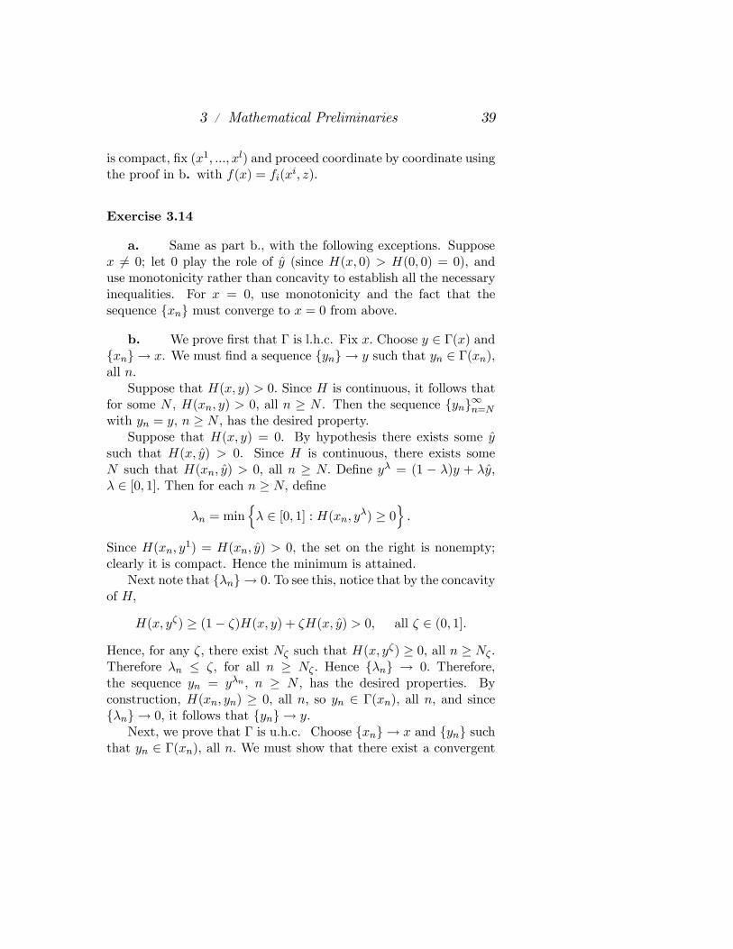
a. Same as part b., with the following exceptions. Supposex 6= 0; let 0 play the role of y (since H(x, 0) > H(0, 0) = 0), anduse monotonicity rather than concavity to establish all the necessaryinequalities. For x = 0, use monotonicity and the fact that thesequence xn must converge to x = 0 from above.
b. We prove first that Γ is l.h.c. Fix x. Choose y ∈ Γ(x) andxn→ x. We must find a sequence yn→ y such that yn ∈ Γ(xn),all n.
Suppose that H(x, y) > 0. Since H is continuous, it follows thatfor some N , H(xn, y) > 0, all n ≥ N . Then the sequence yn∞n=Nwith yn = y, n ≥ N , has the desired property.
Suppose that H(x, y) = 0. By hypothesis there exists some ysuch that H(x, y) > 0. Since H is continuous, there exists someN such that H(xn, y) > 0, all n ≥ N. Define yλ = (1 − λ)y + λy,λ ∈ [0, 1]. Then for each n ≥ N, define
λn = minnλ ∈ [0, 1] : H(xn, yλ) ≥ 0
o.
Since H(xn, y1) = H(xn, y) > 0, the set on the right is nonempty;clearly it is compact. Hence the minimum is attained.
Next note that λn→ 0. To see this, notice that by the concavityof H,
H(x, yζ) ≥ (1− ζ)H(x, y) + ζH(x, y) > 0, all ζ ∈ (0, 1].Hence, for any ζ, there exist Nζ such that H(x, yζ) ≥ 0, all n ≥ Nζ .Therefore λn ≤ ζ, for all n ≥ Nζ . Hence λn → 0. Therefore,the sequence yn = yλn , n ≥ N , has the desired properties. Byconstruction, H(xn, yn) ≥ 0, all n, so yn ∈ Γ(xn), all n, and sinceλn→ 0, it follows that yn→ y.
Next, we prove that Γ is u.h.c. Choose xn→ x and yn suchthat yn ∈ Γ(xn), all n. We must show that there exist a convergent

40 3 / Mathematical Preliminaries
subsequence of yn whose limit point y is in Γ(x). It suffices toshow that the sequence yn is bounded. For if it is, then it hasa convergent subsequence, call it ynk , with limit y. Then, sinceH(xnk , ynk) ≥ 0, all k, (xnk , ynk)→ (x, y), and H is continuous, itfollows that H(x, y) ≥ 0.
Let k·k denote the Euclidean norm in Rm.Choose M < ∞ suchthat kyk < M, all y ∈ Γ(x). Since Γ(x) is compact, this is possi-ble. Suppose yn is not bounded. Then, there exist a subsequenceynk such that N < n1 < n2... and kyk > M + k, all k. DefineS = y ∈ Rm : kyk =M + 1 , which is clearly a compact set. Sincekyk < M , and kynkk > M + k, all k, for any element in the sequenceynk , there exists a unique value λ ∈ (0, 1) such that
kynkk = kλynk + (1− λ)yk+M + 1.
Moreover, since H(xnk , y) > 0 and H(xnk , ynk) ≥ 0, it followsfrom the concavity of H that H(xnk , ynk) > 0, all k. Since by con-struction the sequence ynk lies in the compact set S, it has a con-vergent subsequence; call this subsequence yj and call its limitpoint y. Note that since y ∈ S, kyk = M + 1. Along the chosensubsequence, H(xj , yj) > 0, all j; and (xj , yj)→ (x, y). Since H iscontinuous, this implies that H(x, y) ≥ 0. But then kyk = M + 1, acontradiction.
c. The correspondence can be written in this case as
Γ(x) = y ∈ R : H(x, y) ≥ 0= y ∈ R : 1−max |x| , |y| ≥ 0 .
It can be checked that, at x = 1, Γ(x) is not lower hemi-continuous.Notice that Γ(1) = [−1,+1], which is compact and has a nonemptyinterior, but Γ(1 + 1/n) = 0, for all n > 0.
Exercise 3.15
Let xn, yn be a sequence in A. We need to show that this se-quence has a convergent subsequence. Because X is compact, thesequence xn has a convergent subsequence, say xnk converging

3 / Mathematical Preliminaries 41
to x ∈ X. Because Γ is u.h.c., every sequence xn → x ∈ X, has anassociated sequence yn such that yn ∈ Γ(xn), all n, with a con-vergent subsequence, say ynk whose limit point y ∈ Γ(x). Then,(xn, yn) ∈ A, has a convergent subsequence with limit (x, y) .
Exercise 3.16
a. The correspondence G is
G(x) =
½y ∈ [−1, 1] : xy2 = max
y∈[−1,1]xy2
¾= y ∈ [−1, 1] : y = 0 for x < 0,
y ∈ [−1, 1] for x = 0, y = ±1 for x > 0 .
Thus, G(x) can be drawn as shown in Figure 3.1.
Insert Figure 3.1 About Here.
Then, G(x) is nonempty, and it is clearly compact valued. Further-more, A, the graph of G, is closed in R2 since it is a finite union ofclosed sets. Hence, by Theorem 3.4, G(x) is u.h.c.
To see that G(x) is not l.h.c. at x = 0, choose an increasingsequence xn → x = 0 and y = 1/2 ∈ G(0). In this case, any ynsuch that yn ∈ G(xn) implies that yn = 0, so yn→ 0 6= 1/2.
b. Let be X = R.
Then,
h(x) = maxy∈[0,4]
©max
©2− (y − 1)2, x+ 1− (y − 2)2ªª
= max
½maxy∈[0,4]
[2− (y − 1)2], maxy∈[0,4]
[x+ 1− (y − 2)2]¾
= max 2, x+ 1

42 3 / Mathematical Preliminaries
Hence,
h(x) =
½2 if x ≤ 1x+ 1 if x > 1
Then,
G(x) = y ∈ [0, 4] : y = 1 for x < 1,y ∈ 1, 2 for x = 1, y = 2 for x > 1 ,
which is represented in Figure 3.2.
Insert Figure 3.2 About Here
Evidently, G(x) is nonempty and compact valued. Further, its graphis closed in R2 since the graph is given by the union of closed sets.Thus, G(x) is u.h.c.
However, G(x) is not l.h.c. at x = 1. To see this, let xn → 1for xn > 1 and y = 1 ∈ G(1). It is clear that any sequence yn suchthat yn ∈ G(xn) converges to 2 6= 1.
c. Here,
h(x) = max−x≤y≤x
cos(y) = 1
and henceG(x) = y ∈ [−x, x] : cos(y) = 1 .
Then, since cos(y) = 1 for y = ±2nπ, where n = 0, 1, 2, ..., thecorrespondence G(x) can be depicted as in Figure 3.3.
Insert Figure 3.3 About Here
The argument to show that G(x) is u.h.c. is the same outlined inb. However, G(x) is not l.h.c. at x = ±2nπ, where n = 0, 1, 2, ...;which can be proved using the same kind of construction of sequencesdeveloped before.

4 Dynamic Programmingunder Certainty
Exercise 4.1
a. The original problem was
maxct,kt+1∞t+0
∞Xt=0
βtu(ct)
subject to
ct + kt+1 ≤ f(kt),
ct, kt+1 ≥ 0,
for all t = 0, 1, ... with k0 given. This can be equivalently written,after substituting the budget constraint into the objective function,as
maxkt+1∞t+0
∞Xt=0
βtu[f(kt)− kt+1]
subject to0 ≤ kt+1 ≤ f(kt),
for all t = 0, 1, ... with k0 given. Hence, defining
F (kt, kt+1) = u[f(kt)− kt+1],and
Γ(kt) = kt+1 ∈ R+ : 0 ≤ kt+1 ≤ f(kt) ,we obtain the (SP) formulation given in the text.
43

44 4 / Dynamic Programming under Certainty
b. Note that in this case ct ∈ Rl+ for all t = 0, 1, ... and wecannot simply substitute for consumption in the objective function.Instead, define
Γ(kt) :=nkt+1 ∈ Rl+ : (kt+1 + ct, kt) ∈ Y ⊆ R2l+, ct ∈ Rl+
o,
and
Φ (kt, kt+1) :=nct ∈ Rl+ : (kt+1 + ct, kt) ∈ Y ⊆ R2l+
o.
Then, letF (kt, kt+1) = sup
ct∈Φ(kt,kt+1)u (ct) ,
and the problem is in the form of the (SP).
Exercise 4.2
a. Define xit as the ith component of the l dimensional vectorxt. Hence,
maxixit ≤ θt kx0k .
Let e = (1, ..., 1, ...1) be an l dimensional vector of ones. Hence, thefact that F is increasing in its first l arguments and decreasing in itslast l arguments implies that for all θ
F (x1, x2) ≤ F (x1, 0) ≤ F (θ kx0k e, 0)Then, if θ ≤ 1, F (θt kx0k e, 0) ≤ F (kx0k e, 0) and
limn→∞
∞Xt=0
βtF (xt, xt+1) ≤ limn→∞
∞Xt=0
βtF (kx0k e, 0)
=F (kx0k e, 0)(1− β)
,
as β < 1. Otherwise, if θ > 1, F (θt kx0k e, 0) ≤ θtF (kx0k e, 0) by theconcavity of F and
limn→∞
∞Xt=0
βtF (xt, xt+1) ≤ limn→∞
∞Xt=0
(θβ)tF (kx0k e, 0)
=F (kx0k e, 0)(1− θβ)
,

4 / Dynamic Programming under Certainty 45
as βθ < 1. Hence the limit exists.
b. By assumption, for all x0 ∈ X, F (x1, 0) ≤ θF (x0, 0).Hence
F (xt, xt+1) ≤ F (xt, 0) ≤ θF (xt−1, 0) ≤ ... ≤ θtF (x0, 0).
Then,
limn→∞
∞Xt=0
βtF (xt, xt+1) ≤ limn→∞
∞Xt=0
(θβ)tF (x0, 0)
=F (x0, 0)
1− θβ.
Therefore, the limit exists.
Exercise 4.3
a. Let υ (x0) be finite. Since υ satisfies (FE), as shown inthe proof of Theorem 4.3, for every x0 ∈ X and every ε > 0, thereexists x
˜∈ Π(x0) such that
υ (x0) ≤ un(x˜) + βn+1υ (xn+1) +
ε
2.
Taking the limit as n→∞ gives
υ (x0) ≤ u(x˜) + lim sup
n→∞βn+1υ (xn+1) +
ε
2
≤ u(x˜) +
ε
2.
Sinceu(x)˜≤ υ∗ (x0) ,
for all x˜∈ Π(x0), this gives
υ (x0) ≤ υ∗ (x0) +ε
2,

46 4 / Dynamic Programming under Certainty
for all ε > 0. Hence,υ (x0) ≤ υ∗ (x0) ,
for all x0 ∈ X.If υ(x0) = −∞, the result follows immediately. If υ(x0) = +∞,
the proof goes along the lines of the last part of Theorem 4.3. Henceυ(x0) ≤ υ∗(x0), all x0 ∈ X.
b. Since υ satisfies FE, by the argument of Theorem 4.3, forall x0 ∈ X and x
˜∈ Π(x0)
υ(x0) ≥ un(x˜) + βn+1υ(xn+1).
In particular, for x˜and x
˜
0as described,
υ(x0) ≥ limn→∞un(x˜
0) + limn→∞βnυ(x0n+1)
= u(x˜
0)
≥ u(x˜)
all x˜∈ Π(x0). Hence
υ(x0) ≥ υ∗(x0) = supx˜∈Π(x0)
u(x˜),
and in combination with the result proved in part a., the desiredresult follows.
Exercise 4.4
a. Let K be a bound on F and M be a bound on f. Then
(Tf) (x) ≤ K + βM, for all x ∈ X.
Hence T : B(X)→ B(X).In order to show that T has a unique fixed point υ ∈ B(X) we
will use the Contraction Mapping Theorem. Note that (B(X), ρ) is

4 / Dynamic Programming under Certainty 47
a complete metric space, where ρ is the metric induced by the supnorm.
We will use Blackwell’s sufficient conditions to show that T is acontraction. To prove monotonicity, let f, g ∈ B(X), with f(x) ≤g(x) for all x ∈ X. Then
(Tf)(x) = maxy∈Γ(x)
F (x, y) + βf(y)= F (x, y∗) + βf(y∗)≤ F (x, y∗) + βg(y∗)≤ max
y∈Γ(x)F (x, y) + βg(y) = (Tg)(x),
wherey∗ = arg max
y∈Γ(x)F (x, y) + βf(y) .
For discounting, let a ∈ R. Then
T (f + a)(x) = maxy∈Γ(x)
F (x, y) + β [f(y) + a]= max
y∈Γ(x)F (x, y) + βf(y)+ βa
= (Tf)(x) + βa.
Hence by the Contraction Mapping Theorem, T has a unique fixedpoint υ ∈ B(X), and for any υ0 ∈ B(X),
kTnυ0 − υk ≤ βn kυ0 − υk .
That the optimal policy correspondence G : X → X, where
G(x) = y ∈ Γ(x) : υ(x) = F (x, y) + βυ(y) ,
is nonempty is immediate from the fact that Γ is nonempty and finitevalued for all x. Hence, the maximum is always attained.
b. Note that as F and f are bounded, Thf is bounded.Hence Th : B(X) → B(X). That Th satisfies Blackwell’s sufficientconditions for a contraction can be proven following the same steps

48 4 / Dynamic Programming under Certainty
as in part a. with the corresponding adaptations. Hence, Th is a con-traction and by the Contraction Mapping Theorem it has a uniquefixed point w ∈ B(X).
c. First, note that
wn(x) = (Thnwn)(x)
= F [x, hn (x)] + βwn [hn (x)]
≤ maxy∈Γ(x)
F (x, y) + βwn(y)= (Twn)(x)
= (Thn+1wn)(x).
Hence for all n = 0, 1, ... wn ≤ Twn. Applying the operator Thn+1 toboth sides of this inequality and using monotonicity gives
Twn = Thn+1wn ≤¡Thn+1
¢(Twn) = T
2hn+1wn.
Iterating on this operator gives
Twn ≤ TNhn+1wn.
But wn+1 = limN→∞ TNhn+1wn, for wn ∈ B(X). Hence Twn ≤ wn+1and
w0 ≤ Tw0 ≤ w1 ≤ Tw1 ≤ ... ≤ Twn−1 ≤ Twn ≤ υ.
By the Contraction Mapping Theorem,°°TNwn − υ°° ≤ βN kwn − υk .
Then,
kwn − υk ≤ kTwn−1 − υk ≤ β kwn−1 − υk≤ β kTwn−2 − υk ≤ β2 kwn−2 − υk ≤ ...≤ βn kw0 − υk
and hence wn → υ as n→∞.
Exercise 4.5

4 / Dynamic Programming under Certainty 49
First, we prove that g(x) is strictly increasing. Towards a con-tradiction, suppose that there exists x, x0 ∈ X with x < x0 such thatg(x) ≥ g (x0) . Then as f is increasing, using the first-order condition(5)
βυ0[g(x0)] = U 0[f(x0)− g(x0)]< U 0[f(x)− g(x)] = βυ0[g(x)]
which contradicts υ strictly concave.We prove next that 0 < g(x0)−g(x) < f(x0)−f(x), if x0 > x. Let
x0 > x. As g(x) is strictly increasing, using the first-order conditionwe have
U 0[f(x)− g(x)] = βυ0[g(x)]> βυ0[g(x0)] = U 0[f(x0)− g(x0)].
The result follows from U strictly concave.
Exercise 4.6
a. By Assumption 4.10 kxtkE ≤ α kxt−1kE for all t. Hence
α kxt−1kE ≤ α2 kxt−2kEand
kxtkE ≤ α2 kxt−2kEThe desired result follows by induction.
b. By Assumption 4.10 Γ : X → X is nonempty.Combining Assumptions 4.10 and 4.11,
|F (xt, xt+1)| ≤ B (kxtkE + kxt+1kE)≤ B(1 + α) kxtkE≤ B(1 + α)αt kx0kE
for α ∈ (0,β−1) and 0 < β < 1. So, by Exercise 4.2, Assumption 4.2is satisfied.

50 4 / Dynamic Programming under Certainty
c. By Assumption 4.11 F is homogeneous of degree one, so
F (λxt,λxt+1) = λF (xt, xt+1).
Then
u(λx˜) = lim
n→∞
nXt=0
βtF (λxt,λxt+1)
= λ limn→∞
nXt=0
βtF (xt, xt+1) = λu(x˜).
By Assumption 4.10 the correspondence Γ displays constant returnsto scale. Then clearly x
˜∈ Π(x0) if and only if λx
˜∈ Π(λx0). Hence
υ∗(λx0) = supλx˜∈Π(λx0)
u(λx˜)
= λ supx˜∈Π(x0)
u(x˜)
= λυ∗(x0).
By Assumption 4.11,
|F (xt, xt+1)| ≤ B (kxtkE + kxt+1kE)≤ B (1 + α) kxtkE ≤ B(1 + α)αt kx0kE .
Hence
|υ∗(x0)| =
¯¯ supx˜∈Π(x0)
∞Xt=0
βtF (xt, xt+1)
¯¯
≤ supx˜∈Π(x0)
∞Xt=0
βt |F (xt, xt+1)|
≤∞Xt=0
B(1 + α) (αβ)t kx0kE
=B(1 + α)
1− αβkx0kE .

4 / Dynamic Programming under Certainty 51
Therefore υ∗(x0) ≤ c kx0kE, all x0 ∈ X, where
c =B(1 + α)
1− αβ.
Exercise 4.7
a. Take f and g homogeneous of degree one, and α ∈ R,then f + g and αf are homogeneous of degree one, and clearly k·k isa norm, so H is a normed vector space. We hence turn to the proofthat H is complete. Let fn be a Cauchy sequence in H. Thenfn converges pointwise to a limit function f. We need to showthat fn → f ∈ H where the convergence is in the norm of H. Theproof of convergence, and that f is continuous, are analogous to theproof of Theorem 3.1. To see that f is homogeneous of degree one,note that for any x ∈ X and any λ ≥ 0
f (λx) = limn→∞ fn (λx) = lim
n→∞λfn (x) = λf (x) .
b. Take f ∈ H(X). Tf is continuous by the Theorem of theMaximum. To show that Tf is homogeneous of degree one, noticethat
(Tf)(λx) = supλy∈Γ(λx)
F (λx,λy) + βf(λy)
= supy∈Γ(x)
λ F (x, y) + βf(y)
= λ(Tf)(x),
where the second line follows from Assumption 4.10.
Exercise 4.8
In order to prove the results, we need to add the restriction that fis non-negative, and strictly positive on Rl++. As a counterexamplewithout this extra assumption, letX = R2+ and consider the function
f(x) =
(x1/21 x
1/22 if x2 ≥ x1
0 otherwise.

52 4 / Dynamic Programming under Certainty
This function is clearly not concave, but is homogeneous of degreeone and quasi-concave. To see homogeneity, let λ ∈ [0,∞) and notethat
f(λx) =
(λx
1/21 x
1/22 if x2 ≥ x1
0 otherwise.
= λf(x).
To see quasi-concavity, let x, x0 ∈ X with f(x) ≥ f(x0). If f(x0) = 0the result follows from f non-negative. If f(x0) > 0, then x2 ≥ x1and x02 ≥ x01, and as f(x) is Cobb-Douglas in this range, it is quasi-concave.
a. Pick two arbitrary vectors x, x0 ∈ X, and assume that fis non-negative, and strictly positive on Rl++. We have to considerfour cases:
i) x = x0
ii) x = αx0 for any α ∈ R, and x 6= 0, x0 6= 0iii) x 6= αx0 for any α ∈ R, and x 6= 0, x0 6= 0iv) x 6= x0 and x = 0 or x0 = 0
i) and ii) are trivial.iii) Suppose f(x) ≥ f(x0), then f being homogeneous of degree
one and non-negative implies that f(x)/f(x0) ≥ 1, so there exist anumber γ ∈ (0, 1) such that γf(x) = f(γx) = f(x0). Hence for anyλ ∈ (0, 1) we may write
f(γx) = λf(γx) + (1− λ)f(x0) = f(x0).
By the assumed quasi-concavity of f , for any ω ∈ (0, 1),
f [ωγx+ (1− ω)x0] ≥ ωf(γx) + (1− ω)f(x0).
Then, for any t > 0,
f [tωγx+ t(1− ω)x0] = tf [ωγx+ (1− ω)x0]≥ tωf(γx) + t(1− ω)f(x0)= tωγf(x) + t(1− ω)f(x0).

4 / Dynamic Programming under Certainty 53
For any γ ∈ (0, 1), [1− ω(1− γ)]−1 > 0, hence choosing
t = [1− ω(1− γ)]−1
we get
f
·ωγ
1− ω(1− γ)x+
(1− ω)
1− ω(1− γ)x0¸
≥ ωγ
1− ω(1− γ)f(x) +
(1− ω)
1− ω(1− γ)f(x0),
so if we let θ = ωγ/ [1− ω(1− γ)] , we obtain
f [θx+ (1− θ)x0] ≥ θf(x) + (1− θ)f(x0).
In order to see that the above expression holds for any θ, definegγ : (0, 1)→ (0, 1) by
gγ(ω) =ωγ
1− ω (1− γ),
which is continuous and strictly increasing. Hence the proof is com-plete.
iv) Suppose x0 = 0. Then, f(x0) > 0 or f(x0) = 0. In the for-mer case the proof of iii) applies without change. In the latter casef(x0) = 0, so for any x 6= 0 and θ ∈ (0, 1),
f [θx+ (1− θ)x0] = f(θx) = θf(x) + (1− θ)f(x0).
b. Same proof as in case iii) in part a. assuming f(x) ≥ f(x0)and replacing ≥ by > everywhere else.
c. In order to prove that the fixed point υ of the operatorT defined in (2) is strictly quasi-concave, we need X, Γ, F and βto satisfy Assumptions 4.10 and 4.11. In addition, we need F to bestrictly quasi-concave (see part b.). To show this, let H 0(X) ⊂ H(X)be the set of functions on X that are continuous, homogeneous ofdegree one, quasi-concave and bounded in the norm in (1), and letH 00(X) be the set of strictly quasi-concave functions. Since H 0(X) is

54 4 / Dynamic Programming under Certainty
a closed subset of the complete metric space H(X), by Theorem 4.6and Corollary 1 to the Contraction Mapping Theorem, it is sufficientto show that T [H 0(X)] ⊆ H 00(X).
To verify that this is so, let f ∈ H 0(X) and let
x0 6= x1, θ ∈ (0, 1), and xθ = θx0 + (1− θ)x1.
Let yi ∈ Γ(xi) attain (Tf)(xi), for i = 0, 1, and let F (x0, y0) >F (x1, y1). Then by Assumption 4.10, yθ = θy0 + (1 − θ)y1 ∈ Γ(xθ).It follows that
(Tf)(xθ) ≥ F (xθ, yθ) + βf(yθ)
> F (x1, y1) + βf(y1)
= (Tf)(x1),
where the first line uses (3) and the fact that yθ ∈ Γ(xθ); the seconduses the hypothesis that f is quasi-concave and the quasi-concavityrestriction on F ; and the last follows from the way y0 and y1 wereselected. Since x0 and x1 were arbitrary, it follows that Tf is strictlyquasi-concave, and since f was arbitrary, that T [H 0(X)] ⊆ H 00(X).Hence the unique fixed point υ is strictly quasi-concave.
d. We need X, Γ, F , and β to satisfy Assumptions 4.9, 4.10and 4.11, and in addition F to be strictly quasi-concave. Consideringx, x0 ∈ X with x 6= αx0 for any α ∈ R, Theorem 4.10 applies.
Exercise 4.9
Construct the sequence k∗t ∞t=0 using
kt+1 = g (kt) = αβkαt ,
given some k0 ∈ X. If k0 = 0 we have that k∗t = 0 for all t = 0, 1, ...which is the only feasible policy and is hence optimal. If k0 > 0,then for all t = 0, 1, ... we have that k∗t+1 ∈ intΓ (k∗t ) as αβ ∈ (0, 1) .
LetE (xt, xt+1) := Fy (xt, xt+1) + βFx (xt, xt+1) .

4 / Dynamic Programming under Certainty 55
Then for all t = 0, 1, 2, ... we have that
E¡k∗t , k
∗t+1
¢= β
αk∗α−1t
k∗αt − k∗t+1− 1
k∗αt−1 − k∗t= β
αk∗α−1t
k∗αt − αβk∗αt− 1
k∗αt−1 − αβk∗αt−1
=αβ
k∗t (1− αβ)− 1
k∗αt−1(1− αβ)
=1
k∗αt−1(1− αβ)− 1
k∗αt−1(1− αβ)= 0,
from repeated substitution of the policy function. Hence the Eulerequation holds for all t = 0, 1, ...
To see that the transversality condition holds, let
T (xt, xt+1) = limt→∞βtFx (xt, xt+1) · xt.
Then,
T¡k∗t , k
∗t+1
¢= lim
t→∞βtαk∗α−1t
k∗αt − k∗t+1kt
= limt→∞βt
αk∗αtk∗αt − αβk∗αt
= limt→∞βt
α
(1− αβ)= 0,
where the result comes from the fact that 0 < β < 1.

5 Applications ofDynamic Programmingunder Certainty
Exercise 5.1
a.- c. The answers to parts a. through c. of this questionrequire that Assumptions 4.1 through 4.8 be established. We verifyeach in turn.
A4.1: Here Γ(x) = [0, f(x)], and since by T2 f (0) = 0, 0 ∈Γ (x) for all x, and therefore Γ is nonempty for all x.
A4.2: Here F (xt, xt+1) = U [f(xt) − xt+1]. By U3 and thefact that U : R+ → R, U , and hence F , is bounded below and theresult follows from U1.
A4.3: X = [0, x] ∈ R+ which is a convex subset of R. Referto Exercise 3.13 b. for Γ non-empty and compact valued. By T1 andExercise 3.13, Γ is continuous.
A4.4: We showed above that F is bounded below. By T1-T3 f(xt) − xt+1 is bounded, and hence by assumption U2-U3 Fis bounded above. By U2 and T1, F is continuous. And by U1,0 < β < 1.
A4.5: By U3 and T3, F (·, y) is a strictly increasing function.A4.6: Let x ≤ x0, then by T3, f(x) ≤ f(x0), which implies
that [0, f(x)] ⊆ [0, f(x0)] .
56

5 / Applications of Dynamic Programming 57
A4.7: By T4 f(x)− y is a concave function in (x, y). By U4this implies that F (x, y) is strictly concave in (x, y).
A4.8: Let x, x0 ∈ X, y ∈ Γ(x) and y0 ∈ Γ(x0). Then y ≤ f(x)and y0 ≤ f(x0), which implies, by T4, that
θy + (1− θ)y0 ≤ θf(x) + (1− θ)f(x0)≤ f(θx+ (1− θ)x0).
d. υ(x) is differentiable at x: By Theorems 4.7 and 4.8 andparts b. and c., υ is an increasing and strictly concave function. ByU5, T5 and g(x) ∈ (0, f(x)) , Assumption 4.9 is satisfied. Hence byTheorem 4.11 υ is continuously differentiable and
υ0(x) = Fx[f(x)− g(x)] = U 0[f(x)− g(x)]f 0(x).
0 < g(x) < f(x): A sufficient condition for an interior solution is
limc→0U
0(c) =∞.
To see that g(x) = f(x) is never optimal under this condition, noticethat υ is differentiable for x ∈ (0, x) when g(x) ∈ (0, f(x)). Hence,in this case we have that g(x) satisfies
U 0 [f(x)− g(x)] = βυ0 [g (x)] ,
butlim
g(x)→f(x)U 0 [f(x)− g(x)] =∞,
whilelim
g(x)→f(x)βυ0 [g(x)] <∞,
by the strict concavity of υ.To show that g(x) = 0 is not optimal, assume g(x) = 0, for some
x > 0. Hence, it must be that g(x) = 0 for x < x. But then, forx < x
υ(x) ≡ U [f(x)] + βU(0)
1− β.

58 5 / Applications of Dynamic Programming
Therefore υ is differentiable and
υ0(x) = U 0 [f(x)] f 0(x).
Hence, when x → 0, υ0(x) → ∞, and then g(x) = 0 for x is notpossible.
To see what happens when this condition fails, notice that atthe steady state, we have that g(x∗) < f(x∗), where x∗ stands forthe steady state level of capital. By continuity of g, there is aninterval (x∗ − ε, x∗), such that for any x belonging to that interval,g(x) < f(x). Theorem 4.11 implies that υ is differentiable in thisrange. For any other x, eventually this interval will be reached, oranother point interval that implies g(x) = 0 or g(x) < f(x). Weestablished above that υ is differentiable in those cases, so it mustbe that υ is differentiable everywhere.
e. Let β0 > β. Define T 0 as the operator T using β0 as adiscount factor instead of β, and υk as the kth application of thisoperator.
Applying T 0 to υ(x;β) once (that is, using υ as the inital condi-tion of the iteration) we obtain υ1(x;β
0) and g1(x;β0), where usingthe first-order condition (assuming an interior solution for simplic-ity), g1(x;β0) is defined as the solution y to
U 0[f(x)− y] = β0υ0(y,β).
It is clear that the savings function must increase since the right-hand side increases from β to β0, that is g1(x;β0) > g1(x;β), whichby Theorem 4.11 in turn implies
υ01(x,β0) > υ0(x,β).
By a similar argument, if
υ0k(x;β0) > υ0k−1(x;β
0),
thenυ0k+1(x;β
0) > υ0k(x;β0),
andgk+1(x;β
0) > gk(x;β0).

5 / Applications of Dynamic Programming 59
Hence, gk(x;β0) increases with k. The result then follows from ap-plying Theorem 4.9 to the sequence
©gk(x;β
0)ª∞k=0
since gk(x;β0)→g(x;β0).
Exercise 5.2
a. For f(x) = x, T1 and T3-T5 are easily proved as follows:
T1: To prove that the function f is continuous, we must showthat for every ε > 0 and every x ∈ R+, there exist δ > 0 such that¯
f(x)− f(x0)¯ < ε if¯x− x0¯ < δ.
Choosing δ = ε the definition of continuity is trivially satisfied.
T3: Pick x, x0 ∈ R+, with x > x0, then f(x) = x > x0 =f(x0).
T4: Pick x 6= x0 ∈ R+. Then, for any α ∈ (0, 1),
αf(x) + (1− α)f(x0) = αx+ (1− α)x0 = f [αx+ (1− α)x0],
so f is weakly concave.
T5: For every x ∈ R+,
limε→0
f(x+ ε)− f(x)ε
= 1,
so f is continuously differentiable.
Also, notice that given this technology, there is no growth inthe economy. Hence the maximum level of capital is given by theinitial condition x0 ≥ 0. Therefore, for the nontrivial case where theeconomy starts with a positive level of capital, we can always definex = x0 and restrict attention to the set X = [0, x0]. Given the lineartechnology, it is always possible to mantain the pre-existing capitalstock, hence the desired result follows.

60 5 / Applications of Dynamic Programming
b. The problem can be stated as
maxxt+1∞t=0
∞Xt=0
βt ln(xt − xt+1),
subject to
0 ≤ xt+1 ≤ xt, t = 0, 1, ...,
given x0 ≥ 0.Since lnxt ≤ lnx0 for all t,
ln(xt − xt+1) ≤ ln(xt) ≤ ln(x0).
Then, for any feasible sequence,
∞Xt=0
βt ln(xt − xt+1) ≤ 1
1− βln(x0).
Hence,
υ∗(x) ≤ 1
1− βln(x0),
where υ∗ is the supremum function.Define
υ(x) =1
1− βln(x).
It is clear that υ satisfies conditions (1) to (3) of Theorem 4.14.Define
Tfn(x) = max0≤y≤x
ln(x− y) + βfn(y) .
Then
T υ(x) = max0≤y≤x
½ln(x− y) + β
1− βln(y)
¾=
1
1− βlnx+ ln(1− β) +
β
1− βlnβ,

5 / Applications of Dynamic Programming 61
where the second line uses the fact that the first-order condition ofthe right hand side implies y = βx. Using the same procedure,
T 2υ(x) = max0≤y≤x
½ln(x− y) + β
1− βln(y)
+β
·ln(1− β) +
β
1− βlnβ
¸¾=
1
1− βlnx+ (1 + β)
·ln(1− β) +
β
1− βlnβ
¸and more generally,
Tnυ(x) =1
1− βlnx+
·ln(1− β) +
β
1− βlnβ
¸ nXj=0
βj .
Define υ = limn→∞ Tnυ. Taking the limit of the expressionabove, we have
υ(x) =1
1− βlnx+
1
1− β
·ln(1− β) +
β
1− βlnβ
¸which is clearly a fixed point of T . Hence, by Theorem 4.14, υ = υ∗.
Then, as
Tυ(x) = max0≤y≤x
ln(x− y) + βυ(y) ,
the first-order condition of the right hand side implies that the policyfunction g is given by the expression g(x) = βx.
c. Notice that the only change between the current formu-lation and the one presented in Exercise 5.1 is the linearity of thetechnology. Restricting the state space to X = [0, x0] all the resultsobtained in Exercise 5.1 are still valid under this setup.
Exercise 5.6
a. Let X = R+. Define
Γ(Q) = y : y ≥ Q, y ≤ Q+ q = [Q,Q+ q] .

62 5 / Applications of Dynamic Programming
Since φ(q) =c and limQ→∞ γ(Q) = c it is never profitable to producemore than q.
To show the existence of a unique bounded continuous functionυ satisfying the functional equation
υ(Q) = maxy≥Q
(y −Q) [φ(y −Q)− γ(Q)] + βυ(y)
it is enough to show that the assumptions of Theorem 4.6 are satis-fied. We establish each in turn.
A4.3: X = R+ is a convex subset of Rl. Also, Γ is nonemptysince Q ∈ Γ(Q) for all Q, compact valued since it is a closed intervalin R+, and clearly continuous since it has a continuous lower andupper bound.
A4.4: Let
F (Q, y) = (y −Q) [φ(y −Q)− γ(Q)] .
Then
0 ≤ F (Q, y) ≤ q [φ(0)− γ(Q)] < q [φ(0)− c] <∞.Hence F (Q, y) is bounded. Since φ and γ are continuous functions,F (Q, y) is also continuous. Finally, 0 < β < 1 since r > 0. HenceTheorem 4.6 applies.
To show that Assumption 4.6 does not hold, consider Q < Q0
with Q0 < Q+ q. Then Γ(Q) = [Q,Q+ q] and Γ(Q0) = [Q0, Q0 + q] .Hence,
Γ(Q) ∪ Γ(Q0) = £Q,Q0 + q¤ 6= £Q0, Q0 + q¤ ,which implies that Γ(Q) is not a subset of Γ(Q0).
To show that Assumption 4.7 does not hold, an extra assumptionabout the curvatures of γ and φ is needed. Necessary and sufficientconditions for F (x, y) to be jointly concave in (x, y) are F11, F22 <0, and F11F22 − F 212 > 0. In this example
F (x, y) = (y − x) [φ(y − x)− γ(x)] ,

5 / Applications of Dynamic Programming 63
so
F1(x, y) = − [φ(y − x)− γ(x)]− (y − x) £φ0(y − x) + γ0(x)¤,
F2(x, y) = [φ(y − x)− γ(x)] + (y − x)φ0(y − x),and
F11 = 2£φ0 + γ0
¤+ (y − x) £φ00 − γ00
¤,
F12 = −2φ0 − γ0 − (y − x)φ00,F22 = 2φ0 + (y − x)φ00.
Note that
F11 = F22 + 2γ0 − (y − x) γ00,
F12 = −F22 − γ0.
The assumption that φ+ qφ0 is decreasing implies F22 < 0, and theadditional assumption that γ is decreasing and convex then impliesF11 < 0. To insure that F11F22 − F 212 > 0, we need
0 < F22£F22 + 2γ
0 − (y − x) γ00¤− £F22 + γ0¤2
= −F22 (y − x) γ00 −¡γ0¢2.
The first term is positive, but a joint restriction on γ and φ is neededto insure that it offsets the second term:
[γ0(x)]2
γ00(x)< − £2qφ0(q) + q2φ00(q)¤ , all q, x.
An alternative argument to show that υ is strictly increasing canbe constructed by examining the problem posed in terms of infinitesequences then applying the Principle of Optimality. The Principleholds because under Assumptions 4.3—4.4 we have that Assumptions4.1—4.2 hold.
Consider two initial stocks of cumulative experience Q0 and Q00∈ X with Q0 < Q00. Let Q∗t be the optimal sequence from Q0 anddefine q∗t as the optimal production levels from Q0 by
q∗t = Q∗t+1 −Q∗t .

64 5 / Applications of Dynamic Programming
Then,
υ(Q00) ≥∞Xt=0
βtq∗t£φ(q∗t )− γ
¡Q∗t +Q
00 −Q0
¢¤>
∞Xt=0
βtq∗t [φ(q∗t )− γ(Q∗t )] = υ(Q0),
where the strict inequality comes from the fact that γ is strictlydecreasing. Hence, υ is strictly increasing.
Next, we will show that y∗ ∈ G(Q) implies thaty∗ > argmax
y≥Q(y −Q) [φ(y −Q)− γ(Q)] ≡ y.
Note that y is implicitly determined by
φ(y −Q)− γ(Q) + (y −Q)φ0(y −Q) = 0,or
φ(y −Q) + (y −Q)φ0(y −Q) = γ(Q),
where the left hand side is strictly decreasing in y by the assumptionof strictly decreasing marginal revenue.
On the other hand, y∗ is determined by the first-order condi-tion of the right hand side of the Bellman equation, assuming υ isdifferentiable, (see Theorem 4.11), then
φ(y∗ −Q) + (y∗ −Q)φ0(y∗ −Q) = γ(Q)− βυ0(y∗).
Having shown that υ is increasing, we can conclude that
φ(y∗ −Q) + (y∗ −Q)φ0(y∗ −Q) < γ(Q),
which implies that y∗ > y.
b. S is continuously differentiable since φ is continuouslydifferentiable and integrals are linear operators. Using Leibniz Rule,S 0(q) = φ(q) > 0, and S 00(q) = φ0(q) < 0.
To show that there is a unique bounded and continuous functionw satisfying the functional equation
w(Q) = maxy≥Q
S(y −Q)− (y −Q)γ(Q) + βw(y) ,

5 / Applications of Dynamic Programming 65
let Γ(Q) = [Q,Q+ q] by the same argument given in a. HenceAssumption 4.3 is satisfied.
LetF (Q, y) = S(y −Q)− (y −Q)γ(Q),
then F (Q, y) ≤ S(q) <∞, so F is bounded.Since S and γ are continuous functions, F is a continuous func-
tion, so Assumption 4.4 is also satisfied and the desired result followsfrom Theorem 4.6.
To show that w ≤ S(q)/(1− β), define the operator T by
(Tw)(Q) = maxy∈Γ(Q)
S(y −Q)− (y −Q)γ(Q) + βw(y) .
That T is monotone follows from the fact that if w(Q) > w0(Q) forall Q, then
(Tw)(Q) = maxy∈Γ(Q)
S(y −Q)− (y −Q)γ(Q) + βw(y)
> maxy∈Γ(Q)
©S(y −Q)− (y −Q)γ(Q) + βw0(y)
ª= (Tw0)(Q).
We have shown already that
limn→∞(T
nw0)(Q) = w(Q),
where w(Q) satisfies the Bellman equation. Start with w0(Q) = 0.Then
w1(Q) = maxy∈Γ(Q)
S(y −Q)− (y −Q)γ(Q)≤ S(q),
and applying T to both sides of this inequality we get
(Tw1)(Q) ≤ (TS)(q)
= maxy∈Γ(Q)
S(y −Q)− (y −Q)γ(Q) + βS(q)≤ (1 + β)S(q).

66 5 / Applications of Dynamic Programming
Therefore,
limn→∞(Tw1)(Q) ≤ lim
n→∞(TS)(q) ≤ (1 + β + β2 + ...)S(q),
and hence
w(Q) ≤ S(q)
(1− β),
for all Q ∈ X.
As before, Assumption 4.6 is not satisfied, so in order to showthat w is strictly increasing, pick two arbitrary initial stocks Q0, Q00∈ X with Q0 < Q00. Consider a strictly increasing function w0 and lety∗ be the optimal choice of next period cumulative experience whenQ0 is the current stock and w0 is the continuation value function.Then
(Tw0)(Q0) =©S(y∗ −Q0)− (y∗ −Q0)γ(Q0) + βw0(y∗)
ª,
and
(Tw0)(Q00) ≥ S(y∗ −Q0)− (y∗ −Q0)γ(Q00) + βw0£y∗ −Q0 +Q00
¤> S (y∗ −Q0)− (y∗ −Q0) γ (Q0) + βw0 (y∗)= (Tw0)(Q0),
since w0 is strictly increasing, and γ is strictly decreasing. ThenT maps strictly increasing into strictly increasing functions and byCorollary 1 to the Contraction Mapping Theorem, w(Q) is a strictlyincreasing function.
The proof that any output level that is optimal exceeds the levelthat maximizes current surplus is a straightforward adaptation of theproof outlined in a.
c. Competitive firms take prices and aggregate production asgiven. Normalize the total number of firms to one. The sequentialproblem for an individual firm can be stated as
maxqt∞t=0
∞Xt=0
βtqt [pt − γ(Qt)] .

5 / Applications of Dynamic Programming 67
The equilibrium conditions are
pt = φ (qt)Xi
qit = Qt+1 −Qt.
where we have exploited the fact that under our normalization, ag-gregate production in the industry is qt. The first-order condition ofthe firm’s problem implies zero production at time t if
pt < γ(Qt),
infinite production at t if
pt > γ(Qt),
and indeterminate production at t if
pt = γ(Qt).
After substituting the equilibrium conditions we obtain
pt = φ (Qt+1 −Qt) = γ(Qt).
Since φ and γ are strictly decreasing functions, production is anincreasing function of Q.
As a result, production will rise through time, but since γ is a con-vex function the growth rate has to be declining, with limt→∞ qt = q.Concurrently, the price will be declining through time at a decreasingrate with an asymptote at c since φ(Qt+1 −Qt) declines with Qt.
The equation describing the efficient path of production implies
φ(yE −Q) < γ(Q).
In the competitive equilibrium,
φ(yC −Q) = γ(Q).
Therefore yE > yC as φ is strictly decreasing. Hence the competitiveoutput level is lower.

68 5 / Applications of Dynamic Programming
d. Instead of building a stock of cumulative experience, wehave an initial stock of a nonrenewable resource that will be depletedover time. The recursive formulation of the problem can be statedas
w(Q) = maxy≤Q
S(Q− y)− (Q− y)γ(Q) + βw(y) .Assuming that the cost of extraction γ is strictly increasing and
strictly convex and defining Γ(Q) = [0, Q] which satisfies Assumption4.3, the problem is well defined. All of the proof presented above ap-plies with slight modifications. Posed in terms of infinite sequences,the monopolist’s problem can be stated as
maxQt+1∞t=0
∞Xt=0
βt(Qt −Qt+1) [φ(Qt −Qt+1)− γ(Qt)] ,
subject toQt ≥ Qt+1 t = 0, 1, ...,
with Q0 given.
Exercise 5.7
a. Define
Γ(k) = y : (1− δ)k ≤ y ≤ (1 + λ)k ,and set υ0(k) = 0 for all k. Then for n = 1,
υ1(k) = (Tυ0)(k)
= maxy∈Γ(k)
kφ(y/k) + βυ0(y) = a1k
wherea1 = max
y∈Γ(k)φ(y/k) = φ(1− δ) = 1.
Now assume that υn(k) = (Tnυ0)(k) = ank. To see that theresult holds for n+ 1, note that
υn+1(k) = (Tn+1υ0)(k)
= maxy∈Γ(k)
kφ(y/k) + βυn(y)= max
y∈Γ(k)kφ(y/k) + βany .

5 / Applications of Dynamic Programming 69
There are three cases to consider, depending upon whether the opti-mal choice of y is interior or at a corner.
First, consider the case of an interior solution. The first-ordercondition of the problem is
φ0(y/k) + βan = 0,
and hencey = kφ0−1(−βan).
Plugging this expression into the Bellman equation, we have that
υn+1(k) = kφ£φ0−1(−βan)
¤+ βkφ0−1(−βan)an = an+1k,
wherean+1 = φ
£φ0−1(−βan)
¤+ βφ0−1(−βan)an.
Second, consider the case of a corner solution with y = (1− δ)k,which occurs when
φ0(1− δ) + βan ≤ 0.Plugging y = (1− δ)k into the Bellman equation gives
υn+1(k) = kφ(1− δ) + β(1− δ)kan = an+1k,
wherean+1 = 1 + β(1− δ)an.
Finally, consider the case of a corner solution with y = (1 + λ)k,which occurs when
φ0(1 + λ) + βan ≥ 0.Although we have shown that it is never optimal to choose y =(1+λ)k when there is just one period left in which to work, we cannotrule out corner solutions in other periods without making furtherassumptions about φ and some of the parameters of the problem.Plugging y = (1 + λ)k into the Bellman equation we get
υn+1(k) = kφ(1 + λ) + β(1 + λ)kan = an+1k,
wherean+1 = β(1 + λ)an.

70 5 / Applications of Dynamic Programming
Hence the result is true for n+1 and the result follows by induc-tion.
The proof that an+1 > an for all n is by induction. Note thatwe have shown above that a1 = 1. Next, assume an > an−1. Let yn
denote the optimal choice of next period capital when the worker hasn periods left to work, that is
υn (k) = kφ(yn/k) + βυn−1(yn).
Hence,
an+1k = υn+1 (k) = maxy∈Γ(k)
kφ(y/k) + βυn(y)≥ kφ(yn/k) + βυn(y
n)
= kφ(yn/k) + βanyn
> kφ(yn/k) + βan−1yn = υn (k) = ank,
and the result follows.Next, we establish conditions under which the sequence an∞n=0
is bounded. Notice that either
an+1 = 1 + β (1− δ) an,
an+1 = f(an), or
an+1 = β (1 + λ) an,
and φ0−1 : R− → [(1− δ), (1 + λ)] . Therefore
β (1− δ) ≤ ∂f(an)
∂an= βφ0−1(−βan) ≤ β (1 + λ) ,
and hence the required condition is λ < r.
b. We can show, using the fact that an+1 > an for all n,that if in the nth period it is optimal to invest at the minimumfeasible level (complete depletion), then it is optimal to continueinvesting at the minimum level in future periods (n − 1, n − 2, ...),hence y = (1− δ)k from then on.

5 / Applications of Dynamic Programming 71
>From the first-order conditions of the problem, if minimum fea-sible accumulation is optimal
−φ0(1− δ) > βan
But an > an−1 > an−2...implies that −φ0(1−δ) > βan > βan−1...We can also show that if in the nth period it is optimal to invest
at the maximum feasible level y = (1 + λ)k, then it is optimal toinvest at that level for earlier periods also, namely n+ 1, n+ 2, ...
In this case, from the first-order conditions of the problem
−φ0(1 + λ) < βan
But an+1 > an > ... implies that −φ0(1 + λ) < βan < βan+1...
A plausible path for capital (remember we cannot rule out someweird path without making some further assumptions) would be in-creasing at early stages of the individual’s life, reaching a peak, anddecreasing after that point.
Notice that we can have an interior solution and kt+1 < kt socapital may start decreasing before decreasing at the maximum al-lowed rate. We cannot assure from the first-order conditions thatkt+1 = g(kt) is strictly increasing for an interior solution.
In order to characterize the path of kt corresponding to the regionof interior solutions, from the first-order conditions we have
−φ0(y/k) = βan
hencekt+1 = φ0−1(−βan)kt.
Since an∞n=0 is an increasing sequence, higher a’s imply highervalues for φ0−1, and because φ0−1 goes from ranges of φ0−1 > 1 (forhigh values of a) to ranges of φ0−1 < 1 (for low values of a), whenan → a1 capital may increase at the beginning (φ0−1 > 1) and thengradually decrease (φ0−1 < 1).
The age earning profile will also be be hump-shaped, with a flatsegment at the level of zero earnings for the periods in which it isoptimal to accumulate capital at the rate λ.

72 5 / Applications of Dynamic Programming
Exercise 5.9
a. In order to find exact solutions for υ(k) and g(k) we canuse standard calculus, but this requires that υ satisfies certain prop-erties.
First, notice that f(k) is unbounded, so we cannot apply thestandard theorems for bounded returns. One way to get around thisproblem is by judiciously restricting the state space. Define km as
km =p
qf(km) + (1− δ)km.
That is, if k > km, the output in terms of capital that can be obtainedis less than km. Hence it is never optimal to set kt+1 higher thankm. Set k = max km, k0 . Then, let k ∈ K =
£0, k¤where K is the
restricted state space and let y ∈ Γ(k) = K be the restricted feasiblecorrespondence.
Next, we need to check that υ is differentiable, for which it sufficesto check that the assumptions of Theorem 4.11 are satisfied.
A4.3: Since K =£0, k¤ ⊆ R+, K is a convex subset of R.
Since Γ(k) = K, Γ is nonempty, compact valued and continuous byExercise 3.13. Define
A = (k, y) ∈ K ×K : y ∈ Γ(k) ,
and F : A→ R as
F (k, y) = pf(k)− q [y − (1− δ)k] .
A4.4: Since we have restricted the state space, F is bounded,and clearly continuous. Finally 0 < β < 1 by r > 0.
A4.7: Take two arbitrary pairs (k, y) and (k0, y0) and let θ ∈

5 / Applications of Dynamic Programming 73
(0, 1). Define kθ = θk + (1− θ)k0 and yθ = θy + (1− θ)y0. Then
F (kθ, yθ) = pf(kθ)− qhyθ − (1− δ)kθ
i= pf(θk + (1− θ)k0)−qθy + (1− θ)y0 − (1− δ)[θk + (1− θ)k0]
> θpf(k)− q [y − (1− δ)k]+(1− θ)pf(k0)− q £y0 − (1− δ)k0
¤= θF (k, y) + (1− θ)F (k0, y0),
where the strict inequality is the result of the strict concavity of f.
A4.8: Since Γ(k) =©y : 0 ≤ y ≤ kª for all k it follows trivially
that if y ∈ Γ(k) and y0 ∈ Γ(k0) thenyθ ∈ Γ(kθ) = Γ(k) = Γ(k0) = K.
A4.9: By assumption, f is continuously differentiable. Hence,by Theorem 4.11, υ is differentiable. The Bellman equation for thisproblem is
υ(k) = maxy∈Γ(k)
pf(k)− q[y − (1− δ)k] + βυ(y)
so the Euler equation (Inada conditions rule out corner solutions) is
q = β[pf 0(y∗) + (1− δ)q] (5.1)
where y∗ is the value of y that satisfies this equation. Notice thaty∗ does not depend on the current level of capital, so independentlyof it, it is optimal to adjust to y∗ and stay at that level of capitalforever.
The interpretation of (5.1) is as follows. The left-hand side of theEuler equation measures the marginal cost of increasing the stock ofcapital by one more unit.
The right-hand side measures the marginal benefit of an addi-tional unit of capital when the capital stock is already at the y∗
level. Since it takes one period for the capital to be effective the cur-rent marginal benefit must be discounted. It is composed of a first

74 5 / Applications of Dynamic Programming
term which measures the value of its marginal product and a secondterm which is its scrap value if it is sold next period. Hence,
υ(y∗) = pf(y∗)− q[y∗ − (1− δ)y∗] + βυ(y∗),
which implies that
υ(y∗) =1
1− β[pf(y∗)− qδy∗].
So for any arbitrary k ∈ K,
υ(k) = pf(k)− q[y∗ − (1− δ)k] +β
1− β[pf(y∗)− qδy∗].
Within one period, then, all firms end up with the same capitalstock irrespective of their initial capital endowment. The intuitionbehind this result is that the marginal cost of adjusting capital isconstant, so there is no reason to adjust capital in a gradual fashion.Hence y = g(k) = y∗, a constant function.
The economic interpretation of the absence of a nonnegativityconstraint in gross investment is the existence of perfect capital mar-kets, so investment is reversible.
If we have some upper and lower bounds on investment, the fea-sible correspondence is now
Γ(k) = y : (1− δ)k ≤ y ≤ (1− δ)k + aTo ensure differentiability of the value function, we need to check
Assumptions 4.3 and 4.8.
A4.3: We still maintain the assumption that K = [0, k]. It isclear that Γ(k) is nonempty (y = (1 − δ)k ∈ Γ(k)), compact valuedand continuous.
A4.8: Take two arbitrary pairs (k, y) and (k0, y0) where y ∈Γ(k) and y0 ∈ Γ(k0), and θ ∈ (0, 1), and define kθ and yθ as before.We need to show that yθ ∈ Γ(kθ).
By definition
Γ(kθ) =ny : (1− δ)kθ ≤ y ≤ (1− δ)kθ + a
o.

5 / Applications of Dynamic Programming 75
Note that y ∈ Γ(k) implies that (1− δ)k ≤ y, which implies in turnthat (1 − δ)θk ≤ θy, and θy < (1 − δ)θk + a. Hence θy ∈ Γ(θk).Proceeding in the same fashion it can be shown that (1 − θ)y0 ∈Γ[(1− θ)k0]. Therefore, since (1− δ)kθ ≤ yθ and yθ ≤ (1− δ)kθ + a,Γ is convex.
At this point it would be convenient to show that indeed υ is in-creasing and strictly concave. Unfortunately Γ(k) is not monotone,so we cannot apply Theorem 4.7. To show that υ is strictly increas-ing we will use Corollary 1 of the Contraction Mapping Theorem.Let υ ∈ C 0(k) where C 0(k) is the space of continuous and (weakly)increasing functions. Then,
(Tυ)(k) = maxy∈Γ(k)
pf(k)− q[y − (1− δ)k] + βυ(y)= pf(k)− q[y − (1− δ)k] + βυ(y) ,
where y ∈ argmaxy∈Γ(k) pf(k)− q[y − (1− δ)k] + βυ(y) .Take k > k. Then,
(Tυ)(k) < pf(k) + (1− δ)kq − q[y + (1− δ)(k − k)]+βυ[y + (1− δ)(k − k)]
= pf(k)− q[y − (1− δ)k] + βυ(y)
≤ maxy∈Γ(k)
npf(k)− q[y − (1− δ)k] + βυ(y)
o= (Tυ)(k).
Note that y ∈ Γ(k) since y = y+(1− δ)(k− k) implies that y+(1−δ)k = y + (1 − δ)k and y ∈ Γ(k). Hence T : C 0(k) → C 00(k) whereC 00(k) is the space of continuous and strictly increasing functions.Therefore υ ∈ C 00(k) where υ is the fixed point of T.
That υ is strictly concave follows immediately from f being strictlyconcave and Γ convex, so Theorem 4.8 applies.
Let λ and µ be the Lagrange multiplier for the lower and theupper bounds respectively. Then, the first-order condition of theproblem is
q = βυ0(y) + λ− µ.

76 5 / Applications of Dynamic Programming
Hence, λ > 0 implies υ0(y) < q/β and y = (1 − δ)k; µ > 0 impliesυ0(y) > q/β and y = (1 − δ)k + a; and finally λ = µ = 0 impliesυ0(y) = q/β.
Let kλ and kµ be defined as
υ0 [(1− δ)kλ]] = q/β,
andυ0 [(1− δ)kµ + a] = q/β,
so if the level of capital is higher than kλ the firm has too much ofit, and the only way to of depleting it is by letting it depreciate. Ifthe current level of capital is lower than kµ then the firm wants toaccumulate as much capital as possible, but there is a bound on howmuch capital can be accumulated in a single period.
The policy function is then,
g(k) =
(1− δ)k + a if k ≤ kµ
y∗ if kµ ≤ k ≤ kλ(1− δ)k if k ≥ kλ.
b. Under this new setup the functional equation is
υ(k) = maxy∈Γ(k)
pf(k)− c[y − (1− δ)k] + βυ(y)
The proofs that υ is differentiable, strictly increasing and strictlyconcave are similar to the ones presented in part a. The optimallevel of next period’s capital is implicitly determined by the first-order condition
c0[y − (1− δ)k] = βυ0(y).
Since c is strictly convex and υ is strictly concave there is a uniquey∗ that solves the above equation.
The policy function g(k) is a single valued correspondence (seeTheorem 4.8) and it is nondecreasing. Pick any arbitrary k, k0 withk0 > k. The proof is by contradiction. Suppose g(k0) < g(k). Then,by υ strictly concave,
c0[g(k)− (1− δ)k] = βυ0[g(k)]< βυ0[g(k0)] = c0[g(k0)− (1− δ)k0],

5 / Applications of Dynamic Programming 77
which implies, by c strictly convex, that
0 < (1− δ)(k0 − k) < g(k0)− g(k),
a contradiction.Also note that
c0[g(k)− (1− δ)k] > c0[g(k0)− (1− δ)k0]
implies that
(1− δ) >g(k0)− g(k)(k0 − k) ,
hence the policy function has a slope that is strictly less than one.The Envelope Condition is
υ0(k) = pf 0(k) + (1− δ)c0[y − (1− δ)k].
Combining it with the first-order condition we get the Euler equation
c0[y − (1− δ)k] = β©pf 0(y) + (1− δ)c0[y0 − (1− δ)y]
ª.
Notice that, in contrast with the Euler equation obtained in a., nowthe marginal cost of investing is no longer constant. Hence the steadystate capital level k∗ satisfies
c0(δk∗) =β
1− β(1− δ)pf 0(k∗).
Notice that in this case, capital will adjust slowly to this level.
c. Let φ(k) = argmaxl≥0 pF (k, l)− wl . For Π and φ tobe well defined functions, we need the maximum to exist and φ tobe single valued. If F (k, l) is a continuous function for all pairs(k, l) ∈ K × L, then Π and φ will be continuous functions. If, inaddition, F (k, l) is strictly concave in l, then φ will be single valued.
We consider each property ofΠ in turn. ForΠ(0) we need F (0, l) =0 for all l. For then
Π(0) = maxl∈L(k)
−wl = 0,

78 5 / Applications of Dynamic Programming
and the optimal choice of l is zero. To show that limk→0Π0(k) =∞and limk→∞Π0(k) = 0, we need Inada conditions for k on F (k, l).By the Envelope Condition Π0(k) = pFk(k, l) so it is enough thatlimk→0 Fk(k, l) = ∞ and limk→∞ Fk(k, l) = 0. To show that Πstrictly concave we need F (k, l) to be strictly concave.
Exercise 5.10
a. Define
Π(k0) = kt+1∞t=0 : (1− δ)kt ≤ kt+1 ≤ (1 + α)kt, t = 0, 1, ....
Let
k∗t ∞t=0 ∈ arg maxkt∞t=0∈Π(k0)
∞Xt=0
βt pF (kt, kt+1)− q[kt+1 − (1− δ)kt ,
and λ > 0. Then,
υ∗(λk0) ≥∞Xt=0
βt©pF (λk∗t ,λk
∗t+1)− q[λk∗t+1 − (1− δ)λk∗t
ª= λυ∗(k0).
Now let©kλ∗tª∞t=0
be optimal from λk0. Then, clearly,©λ−1kλ∗t
ª∞t=0
is feasible from k0, and
υ∗(k0) ≥∞Xt=0
βt½pF (
1
λk∗t ,
1
λk∗t+1)− q[
1
λk∗t+1 − (1− δ)
1
λk∗t
¾=
1
λυ∗(λk0),
which completes the proof.
b. We will prove that there is a function υ satisfiying thefunctional equation that is homogeneous of degree one. For that, wehave to check that Assumptions 4.10 and 4.11 are satisfied.
LetΓ(k) = y ∈ R+ : (1− δ)k ≤ y ≤ (1 + α)k .

5 / Applications of Dynamic Programming 79
Clearly, the graph of Γ is a cone.Also,
y
k− 1 ≤ α.
Hence, Assumption 4.10 is satisfied.To see that Asumption 4.11 is also satisfied, notice that
pF (k, y)− q [y − (1− δ)k] ≤ pF (k, (1− δ)k) = pF (1, (1− δ))k.
By Theorem 4.13 the desired result follows.
c. Since the return function and the correspondence describ-ing the feasible set are constant returns to scale, Assumption 4.4 nolonger holds. Here, imposing a bound on the state space is not agood idea. Instead, the strategy will be to prove that the structureof the model satisfy Assumptions 4.10—4.11 and then to make use ofTheorem 4.13.
DefineH(k, y) = pF (k, y)− q[y − (1− δ)k].
A 4.10: K is a convex cone since K = R+ ⊆ Rl.If y ∈ Γ(k) then λy ∈ Γ(λk) since
Γ(k) = y : (1− δ)k ≤ y ≤ (1 + α)k .
Also, y ≤ γk for all k ∈ K for some γ ∈ ¡0,β−1¢. Sincey ≤ (1 + α)k,
and(1 + α)k ≤ γk ≤ β−1k,
is needed, we need to assume that (1 + α)β ≤ 1. Notice that theassumption about the marginal adjustment cost, as the rate of growthof capital approaches α > 0, allows the use of the weak inequality.
A 4.11: β ∈ (0, 1).H : R+ ×R+ → R+ is continuous and homogeneous of degree
one. It follows directly from the assumptions about F.

80 5 / Applications of Dynamic Programming
Since F is nonnegative, decreasing in y and homogeneous of de-gree one,
pF (k, y) ≤ pF [k, (1− δ)k]
= pkF [1, (1− δ)].
This implies that
|H(k, y)| ≤ pkF [1, (1− δ)] + q(1− δ)k + qy.
LetB = max pF [1, (1− δ)] + q(1− δ), q ,
then |H(k, y)| ≤ B(|k|+ |y|).
Hence, we can define the operator
(Tυ)(k) = maxy∈Γ(k)
H(k, y) + βυ(y) ,
and by Theorem 4.13, υ, the unique fixed point of the operator T, ishomogeneous of degree one and the optimal policy correspondence
G = y ∈ Γ(k) : υ∗(k) = pF (k, y)− q[y − (1− δ)k] + βυ∗(y) ,
is compact valued, u.h.c. and homogeneous of degree one. The quasi-concavity of F implies that G is single valued.
Since G is homogeneous of degree one, it must be the case thaty ∈ G(k) implies that y = θk for some θ ∈ [(1− δ), (1 + α)]. Also, υhomogeneous of degree one implies that υ(k) = Ak, therefore
Ak = maxθpF (1, θ)− q[θ − (1− δ)] + βAθ k,
so θ∗ = argmaxθ pF (1, θ)− q[θ − (1− δ)] + βAθ is defined by
pFθ(1, θ∗)− q + βA = 0,
and
A =pF (1, θ∗ − q[θ∗ − (1− δ)]
1− βθ∗.

5 / Applications of Dynamic Programming 81
Now
υ∗(k0) =∞Xt=0
βtH(k∗t , k∗t+1) ≤ H[1, (1− δ)]k0
∞Xt=0
[β(1 + α)]t
so imposing β(1+α) < 1 the hypothesis of Theorems 4.2 and 4.3 aresatisfied and the connection between the functional equation and thesequential problem can then be established.
Also, the strict quasi-concavity of F allows us to conclude thatυ is strictly quasi-concave (see Exercise 4.8) since the operator Tpreserves quasi-concavity.
Assumptions 4.9-4.11 are satisfied and F is strictly quasi-concave,so by Exercise 4.8 d., υ is differentiable.
Exercise 5.11
a. To prove boundedness, let B ∈ R and take any c ∈ L.Then, U(ct) ≤ B for all t implies that
u(c) =∞Xt=0
βtU(ct)
≤∞Xt=0
βtB =B
1− β.
To prove continuity, let c ∈ L. We need to show that for everyc0 ∈ L and ε > 0 there is a δ0 > 0 with |u(c0)− u(c)| < ε wheneverkc0 − ckL < δ0.
Equivalently, we need to show that for some sequence cn∞n=1,where cn ∈ L for all n, and cn → c in k·kL norm, |u(cn)− u(c)|→ 0.
Clearly,
|u(cn)− u(c)| =
¯¯∞Xt=0
βtU(cnt )−∞Xt=0
βtU(ct)
¯¯
≤∞Xt=0
βt |U(cnt )− U(ct)|
=NXt=0
βt |U(cnt )− U(ct)|+∞X
t=N+1
βt |U(cnt )− U(ct)| .

82 5 / Applications of Dynamic Programming
for any N.Fix ε. Because U (·) ≤ B,
|U(cnt )− U(ct)| ≤ 2B.
Choose N such that for all N ≥ N,∞X
t=N+1
βt¯U(c0t)− U(ct)
¯ ≤ βN+12B
1− β<
ε
2.
For the first part of the sequence, we know that c0t → ct. Hence,choose n such that for all n ≥ n
|U(cnt )− U(ct)| ≤(1− β)
(1− βN+1)
ε
2,
as k·kL convergence implies pointwise convergence.Then, if n > n and N > N ,
|u(cn)− u(c)| <NPt=0
βt(1− β)
(1− βN+1)
ε
2+
ε
2= ε.
Since ε was arbitrarily chosen, this completes the proof.
b. S is complete. Straightforward adaptation of the proofoutlined in Exercise 3.6.
To see that it is not true that limn→∞ |u (c)− u (cn)| = 0 for allu ∈ S, consider
u (c) = inftct.
Let c ∈ L be a sequence with elements ct = 1 for all t. But then,|u (c)− u (cn)| = 1 for all n, and hence limn→∞ |u (c)− u (cn)| 6= 0.
c. We first check that T satisfies the Blackwell’s sufficientconditions for a contraction. To show that T satisfies monotonicity,let u, υ ∈ S with u(c) > υ(c) for all c. Then
(Tu)(c) = U(c0) + βu(1c)
> U(c0) + βυ(1c) = (Tυ)(c).

5 / Applications of Dynamic Programming 83
To show discounting, note that
[T (u+ a)](c) = U(c0) + β[u(1c) + a]
= U(c0) + βu(1c) + βa
= (Tu)(c) + βa.
Hence the operator T : S → S is a contraction and thereforeu(c) = U(c0) + βu(1c) where u is the unique fixed point of T. Noticethat u(1c) = U(c1) + βu(2c). Hence
u(c) = U(c0) + βU(c1) + β2u(2c).
Continuing the recursion in this fashion, u(c) =P∞t=0 β
tU(ct).
d. For any u, υ ∈ S, the fact that kTWu− TWυk ≤ β ku− υkfollows immediately from the definition of TW and W3. Hence, TW isa contraction and the existence of a unique fixed point uW is impliedby the Contraction Mapping Theorem. It is also a consequence ofthe Contraction Mapping theorem that
kTnWu0 − uk ≤ βnB
1− β, (5.2)
where B is an upper bound for W.To prove that |uW (c)− uW (cn)| ≤ βn kuWk , define unW (c) =
uW (cn). Then, for any c ∈ L,
unW (c) = u(c0, c1, ..., cn−1, 0, 0, ...)= W (c0, uW (c1, ..., cn−1, 0, 0, ...))= W (c0,u
n−1W (1c)).
while uW (c) = W [c0, uW (1c)], hence, by the contraction property,W3,
kuW − unWk < β°°uW − un−1W
°°≤ β2
°°uW − un−2W
°°...
≤ βn°°uW − u0W°°

84 5 / Applications of Dynamic Programming
To complete the proof, we need u0(c) = u(0, 0, ...) = 0, which is trueby W1 and the definition of TW .
By W4 observe that TW takes increasing functions into increas-ing functions. Applying (5.2) to an increasing initial guess u0 theargument is complete.
To prove the concavity of uw we prove first that if u ∈ S isconcave, so is Twu. Take c, c0 ∈ L, θ ∈ (0, 1) and define cθ = θc +(1− θ)c0. Then,
θ(TWu)(c) + (1− θ)(TWu)(c0)
= θW [c0, u(1c)] + (1− θ)W [c00, u(1c0)]
≤ W [θc0 + (1− θ)c00, θu(1c) + (1− θ)u(1c0)]
≤ W [cθ0, u(1cθ)]
= (TWu)(cθ)
where the first inequality follows from the concavity of W and thesecond from the assumed concavity of u and the assumption that Wis increasing in all arguments. To complete the proof, use Corollary1 of the Contraction Mapping Theorem for an initial u0 concave andapply (5.2).
e. The utility function can be written as
uW (c) =W (c0, uW (1c)).
Hence the marginal rate of substitution between ci,t and cj,t+k isgiven by
W2[ct, uw(t+1c)]W1j [ct+k, uw(t+k+1c)]
W1i[ct, uw(t+1c)],
where W1i[ct, uw(t+1c)] is the partial derivative of W1 with respectto the i’th good in period t, and W2 is the partial derivative of Wwith respect to the second argument.

6 Deterministic Dynamics
Exercise 6.1
a. Pick any k ∈ (0, k]. To see that g(k) ∈ (0, k), supposeg(k) = 0. Then,
U 0[f(k)] ≥ βυ0(0) = βU 0[f(0)− g(0)]f 0(0)
but the left-hand side is finite while the right-hand side is not. There-fore, it cannot be optimal to set g(k) = 0.
Similarly, suppose g(k) = k. Because k ∈ (0, k], and consumptionis nonnegative, it must be that k = k. Hence,
U 0[f(k)− k] ≤ βυ0(k) = βU 0[f(k)− g(k)]f 0(k),
but the left-hand side of the inequality stated above is not finite.On the other hand, feasibility requires that g(k) ≤ k. If g(k) = k,this implies zero consumption ever after, which is suboptimal. Henceg(k) < k. But
∞ = U 0(0) = U 0[f(k)− k] ≤ βU 0[f(k)− g(k)]f 0(k),
and the right-hand side is finite, a contradiction.Since g (k) ∈ ¡0, k¢, we can use theorem 4.11 to prove that υ is
differentiable and derive (2) and (3) .
b. Pick k, k0 ∈ (0, k] with k < k0. The proof is by contra-diction. Suppose g(k) ≥ g(k0). Then, υ strictly concave implies
U 0[f(k)− g(k)] = βυ0[g(k)] ≤ βυ0[g(k0)] = U 0[f(k0)− g(k0)].
85

86 6 / Deterministic Dynamics
Hence, by U strictly concave,
f(k)− g(k) ≥ f(k0)− g(k0).Then, f strictly increasing implies
g(k0)− g(k) ≥ f(k0)− f(k) > 0and so g(k0) > g(k), a contradiction.
Exercise 6.2
a. Towards a contradiction, pick k, k0 ∈ [0, 1] with k < k0.Suppose g(k0) ≥ g(k). For this specific case, (7) is given by
α
"(1− g (k))
µk
1− g(k)¶θ#α−1
×"µ
k
1− g(k)¶θ
− θk
1− g(k)µ
k
1− g(k)¶θ−1#
= βυ0[g(k)].
As υ is strictly concave, we have
α
"1− g(k0))
µk0
1− g(k0)¶θ#α−1
×"µ
k0
1− g(k0)¶θ
− θk0
1− g(k0)µ
k0
1− g(k0)¶θ−1#
≤ α
"(1− g(k))
µk
1− g(k)¶θ#α−1
×"µ
k
1− g(k)¶θ
− θk
1− g(k)µ
k
1− g(k)¶θ−1#
,
and after some straightforward algebra,
1 <k0
k<
·1− g(k0)1− g(k)
¸γ,

6 / Deterministic Dynamics 87
where
γ = −·(1− θ)(α− 1)− θ
θα
¸> 0.
Hence,1− g(k0)1− g(k) > 1,
and so g(k0) < g(k), a contradiction.
Exercise 6.3
a. To see that g maps [0, 1] into itself, note that g(0) =g(1) = 0 and that g(xt) is a quadratic equation with a maximum atxt+1 = 1 when xt = 1/2. Figure 6.1 shows xt+1 as a function of xton the interval [0, 1] . The stationary points are the values of x thatsolve x = 4x− 4x2, which are x = 0, and x = 3/4.
Insert Figure 6.1 About Here
b. The function g2(xt) is obtained by simply plugging xt+1 =g(xt) = 4xt − 4x2t into g(xt+1) = 4xt+1 − 4x2t+1.
Hence,
xt+2 = g2(xt) = 4£4xt − 4x2t
¤− 4 £4xt − 4x2t ¤2= 16xt − 80x2t + 128x3t − 64x4t ,
and so g2(0) = 0, g2(1/4) = 3/4, g2(1/2) = 0, g2(3/4) = 3/4, g2(1) =0. Figure 6.2 shows the presence of two-cycles. The four stationarypoints are 0, 0.3455, 0.75, 0.9045 .
Insert Figure 6.2 About Here

88 6 / Deterministic Dynamics
When xt = 0 or xt = 3/4 we know from part a. that xt+1 = 0or xt+1 = 3/4, respectively. Hence, those points cannot represent atwo-cycle. Similarly, when xt = 0.3455 or xt = 0.9045 we know frompart a. that xt+1 6= 0.3455 or xt+1 6= 0.9045 respectively, but wealso know from above that xt+2 = 0.3455 or xt+2 = 0.9045, thereforethose stationary points are our candidates for a two-cycle.
Starting the system at x = 0.3455 or x = 0.9045 we can seethat the system oscillates between those two numbers, showing thepresence of a two-cycle.
The function g3(x) can be obtained in a similar fashion.
Exercise 6.4
The sufficient condition for (8) to hold is
bd− (1 + β)2c2
4β≥ 0.
In this setup, we can write the right-hand side of (8) as
β(x− x)[b(x− x) + c(y − x)] + (y − x) [c(x− x) + d(y − x)]
orbβ(x− x)2 + (1 + β)c(x− x)(y − x) + d(y − x)2.
Adding and substracting·(1 + β)2c2
4bβ
¸(y − x)2
to the above expression to “complete the square” we obtain
bβ[(x− x)2 + (1 + β)c
bβ(x− x) (y − x) + (1 + β)2c2
4bβ(y − x)2]
+[d− (1 + β)2c2
4bβ] (y − x)2
= bβ
·(x− x) + (1 + β)c
2bβ(y − x)
¸2+1
b[bd− (1 + β)2c2
4β] (y − x)2 ,

6 / Deterministic Dynamics 89
so a sufficient condition for this expression to be negative is that
bd− (1 + β)2c2
4β≥ 0.
Exercise 6.5
A matrix is nonsingular if and only if its determinant is not equalto zero. We are going to show that this is the case for A and (I −A) .
Recall that the determinant of a partitioned matrix
C =
·C11 C12C21 C22
¸can be written (if C11 and C22 are invertible) as
det(C) = |C22| ·¯C11 − C12C−122 C21
¯= |C11| ·
¯C22 − C21C−111 C12
¯.
For the case of A, we can write its determinant as
det (A) = |J | · ¯−J−1K ¯= cdet (K)
= c¯−β−1F−1xy F
0xy
¯= cb
= β−l
where c = (−1)l , b = (−β)−l.Similarly, we can write the determinant of (I −A) as
det(I −A) = |I − J −K|=
¯I − (−β−1F−1xy (Fyy + βFxx))− (−β−1F−1xy F 0xy)
¯=
¯β−1F−1xy (βFxy + Fyy + βFxx + F
0xy)¯
=¯β−1F−1xy
¯ · ¯βFxy + Fyy + βFxx + F0xy
¯.
Therefore, F−1xy and (βFxy+Fyy+βFxx+F 0xy) nonsingular impliesthat (I −A) nonsingular.

90 6 / Deterministic Dynamics
Exercise 6.6
a. The characteristic polynomial for A is
λ2 + λβ−1F−1xy (Fyy + βFxx) + β−1 = 0.
Hence,
λ1,λ2 =−β−1F−1xy (Fyy + βFxx)±
qβ−2F−2xy (Fyy + βFxx)2 − 4β−12
,
and for (λ1,λ2) to both be real it must be that
(Fyy + βFxx)2 ≥ 4βF 2xy.
Also, F strictly concave implies that Fxx < 0 and FyyFxx > F 2xy.Hence it is enough to show that
(Fyy + βFxx)2 ≥ 4βFyyFxx.
But
F 2yy − 2βFxxFyy + F 2xx= (Fyy − βFxx)
2
= (βFxx − Fyy)2 ≥ 0.
b. The result comes from simple inspection of the equationdetermining (λ1,λ2). It is obvious from the result obtained in a. that
λ1 =−β−1F−1xy (Fyy + βFxx) +
qβ−2F−2xy (Fyy + βFxx)2 − 4β−12
> 0
To see that λ2 > 0, it is straightforward that if λ2 < 0 then
−β−1F−1xy (Fyy + βFxx) <qβ−2F−2xy (Fyy + βFxx)2 − 4β−1,
which implies
β−2F−2xy (Fyy + βFxx)2 < β−2F−2xy (Fyy + βFxx)
2 − 4β−1,

6 / Deterministic Dynamics 91
a contradiction with β > 0.
c. The proof parallels the argument in b.
Exercise 6.7
a. Actually, Assumption 4.9 is not needed for uniqueness ofthe optimal capital sequence.
A4.3: K = [0, 1] ⊆ Rl and the correspondenceΓ(k) = y : y ∈ K
is clearly compact-valued and continuous.
A4.4: F (k, y) = (1−y)(1−θ)αkθα is clearly bounded in K, andit is also continuous. Also, 0 ≤ β ≤ 1.
A4.7: Clearly F is continuously differentiable, then
Fk = θα(1− y)(1−θ)αkθα−1Fy = −(1− θ)α(1− y)(1−θ)α−1kθαFkk = θα(1− y) (θα− 1)(1−θ)α kθα−2 < 0Fyy = (1− θ)α[(1− θ)α− 1](1− y)(1−θ)α−2kθα < 0Fxy = −θα (1− θ)α(1− y)(1−θ)α−1kθα−1 < 0,
and FkkFyy − F 2xy > 0, hence F is strictly concave.
A4.8: Take two arbitrary pairs (k, y) and (k0, y0) and 0 < π <1. Define kπ = πk + (1 − π)k0, yπ = πy + (1 − π)y0. Then, sinceΓ(k) = y : 0 ≤ y ≤ 1 for all k it follows trivially that if y ∈ Γ(k)and y0 ∈ Γ(k0) then yπ ∈ Γ(kπ) = Γ(k) = Γ(k0) = K.
A4.9: Define A = K×K as the graph of Γ. Hence F is contin-uously differentiable because U and f are continuously differentiable.The Euler equation is
α(1− θ)(1− kt+1)(1−θ)α−1kθαt = βαθ (1− kt+2)(1−θ)α kθα−1t+1 .

92 6 / Deterministic Dynamics
b. Evaluating the Euler equation at kt+1 = kt = k∗, we get
(1− θ)k∗ = βθ (1− k∗) ,
or
k∗ =βθ
1− θ + βθ.
c. From the Euler equation, define
W (kt, kt+1, kt+2)
≡ α(1− θ)(1− kt+1)(1−θ)α−1kθαt−βαθ (1− kt+2)(1−θ)α kθα−1t+1
= 0.
Hence, expanding W around the steady state
W (kt, kt+1, kt+2) = W (k∗, k∗, k∗) +W1(k∗) (kt − k∗)
+W2(k∗) (kt+1 − k∗) +W3(k
∗) (kt+2 − k∗) ,
where
W1(k∗) = α2(1− θ)θ(1− k∗)(1−θ)α−1 (k∗)θα−1 ,
W2(k∗) = −α(1− θ) [(1− θ)α− 1] (1− k∗)(1−θ)α−2 (k∗)θα
−βθα(θα− 1) (1− k∗)(1−θ)α (k∗)θα−2,W3(k
∗) = βθα2(1− θ) (1− k∗)(1−θ)α−1 (k∗)θα−1.
Normalizing byW3(k∗) and using the expression obtained for the
steady state capital we finally get
β−1 (kt − k∗) +B (kt+1 − k∗) + (kt+2 − k∗) = 0,
where
B =1− α(1− θ)
α(1− θ)+1− αθ
αθβ.
That both of the characteristic roots are real comes from the factthat the return function satisfies Assumptions 4.3-4.4 and 4.7-4.9 andit is twice differentiable, so the results obtained in Exercise 6.6 apply.

6 / Deterministic Dynamics 93
To see that λ1 = (βλ2)−1 it is straightforward from the fact that
λ1λ2 =
Ã(−B) +
pB2 − 4β−12
!Ã(−B)−
pB2 − 4β−12
!
=(−B)2 − (B2 − 4β−1)
4= β−1.
To see that λ1 + λ2 = −B, just notice that
λ1 + λ2 =(−B) +
pB2 − 4β−12
+(−B)−
pB2 − 4β−12
= −B.
Then, λ1λ2 > 0 and λ1+λ2 < 0 implies that both roots are negative.In order to have a locally stable steady state k∗ we need one of
the characteristic roots to be less than one in absolute value. Giventhat both roots are negative, this implies that we need λ1 > −1, or
−B +qB2 − 4β−1 > −2,
which after some straightforward manipulation implies
B >1 + β
β.
Substituting for B we get
1− θ + θβ
2θ(1 + β)(1− θ)> α,
or equivalently
β >(2θα− 1)(1− θ)
[1− 2α(1− θ)]θ.
d. To find that k∗ = 0.23, evaluate the equation for k∗ ob-tained in b. at the given parameter values. To see that k∗ is un-stable, evaluate λ1 at the given parameter values. Notice also thatthose parameter values do not satisfy the conditions derived in c.

94 6 / Deterministic Dynamics
e. Note that since F is bounded, the two-cycle sequence sat-isfies the transversality conditions
limt→∞βtF1(x, y) · x = 0 and
limt→∞βtF1(x, y) · y = 0,
for any two numbers x, y ∈ [0, 1], x 6= y. Hence, by Theorem 4.15, ifthe two cycle (x, y) satisfies
Fy(x, y) + βFx(y, x) = 0 and
Fy(y, x) + βFx(x, y) = 0,
it is an optimal path.Conversely, if (x, y) is optimal and the solution is interior, then
it satisfies
Fy(x, y) + βυ0(y) = 0 and υ0(y) = Fx(y, x),Fy(y, x) + βυ0(x) = 0 and υ0(x) = Fx(x, y),
and hence it satisfies the Euler equations stated in the text.Notice that the pair (x, y) defining the two-cycle should be re-
stricted to the open interval (0, 1).
f. We have that
Fy(x, y) + βFx(y, x) = βαθyαθ−1(1− x)α(1−θ)−α(1− θ)xαθ(1− y)α(1−θ)−1,
and
Fy(y, x) + βFx(x, y) = βαθxαθ−1(1− y)α(1−θ)−α(1− θ)yαθ(1− x)α(1−θ)−1
The pair (0.29, 0.18) makes the above set of equations equal tozero, and from the result proved in part e. we already know this isa necessary and sufficient condition for the pair to be a two-cycle.

6 / Deterministic Dynamics 95
g. Define
E1 (kt, kt+1, kt+2, kt+3) ≡ −α(1− θ)kt+1αθ(1− kt+2)α(1−θ)−1
+βαθkαθ−1t+2 (1− kt+3)α(1−θ)= −α(1− θ)xαθ(1− y)α(1−θ)−1
+βαθyαθ−1(1− x)α(1−θ)= 0
E2 (kt, kt+1, kt+2, kt+3) ≡ −α(1− θ)ktαθ(1− kt+1)α(1−θ)−1
+βαθkαθ−1t+1 (1− kt+2)α(1−θ)= −α(1− θ)yαθ(1− x)α(1−θ)−1
+βαθxαθ−1(1− y)α(1−θ)= 0.
Let Eji be the derivative of Ej with respect to the ith argument.
Then, the derivatives are
E11 = 0,
E12 = −α2θ(1− θ)xαθ−1(1− y)α(1−θ)−1,E13 = −α(1− θ)xαθ[α(1− θ)− 1](1− y)α(1−θ)−2
+βαθ(αθ − 1)yαθ−2(1− x)α(1−θ),E14 = βαθyαθ−1(1− x)α(1−θ)−1,E21 = −α2θ(1− θ)yαθ−1(1− x)α(1−θ)−1,E22 = −α(1− θ)yαθ[α(1− θ)− 1](1− x)α(1−θ)−2
+βαθ(αθ − 1)xαθ−2(1− y)α(1−θ),E23 = βαθxαθ−1(1− y)α(1−θ)−1,E24 = 0.
Using the fact that kt+2 = kt in E1, expand this system around(0.29,0.18). Denoting by K deviations around the stationary pointK, we can express the linearized system as
Kt/2+1 =
·kt+3kt+2
¸= H
·kt+1kt
¸= HKt/2
where
H =
·E14 00 E23
¸−1 ·E12 E11E22 E21
¸.

96 6 / Deterministic Dynamics
By evaluating H for the given parameters, it can be verified thatthe system is unstable around the stationary point K = (0.29, 0.18).
Exercise 6.9
a. To show that the functional equation
υ(x) = maxy∈[0,αx]
nShxφ³yx
´i− θ [y − (1− δ)x] + βυ(y)
ohas a unique continuous bounded solution, it is sufficient to checkthat the assumptions of Theorem 4.6 are satisfied.
A4.3: X = R+ ⊆ Rl. Define the correspondence
Γ(x) = y ∈ X : 0 ≤ y ≤ αx .
Hence Γ is nonempty because y = 0 ∈ Γ for all x ∈ X. It is alsoclearly compact-valued and continuous (see Exercise 3.13a.).
A4.4: Define
F (x, y) = Shxφ³yx
´i− θ [y − (1− δ)x] .
Hence F is a bounded and continuous function by S bounded andcontinuous and x ∈ R+. Also, β ∈ (0, 1) . Notice that S is homo-thetic, but not necessarily homogeneous in (x, y). Hence Theorem4.6 applies.
Next, we prove that υ, the unique solution to the functional equa-tion above, is strictly increasing and strictly concave.
A4.5: F (x, y) strictly increasing in x follows from S beingstrictly increasing in q and q strictly increasing in x (the last factimplied by φ being nonnegative and strictly decreasing).
A4.6: Γ is monotone. Pick two arbitrary x, x0 ∈ X with x ≤x0. Then, if 0 ≤ y ≤ αx, we have 0 ≤ y ≤ αx0 and hence Γ(x) ⊆ Γ(x0).
Therefore, by Theorem 4.7, υ is strictly increasing.

6 / Deterministic Dynamics 97
A4.7: By assumption S and φ are strictly concave functions.As F is a composition of weakly concave and strictly concave func-tions, F is strictly concave.
A4.8: Pick two arbitrary pairs (x, y) and (x0, y0) where y ∈Γ(x) and y0 ∈ Γ(x0), for 0 < π < 1. Define xπ and yπ as be-fore. We need to show that yπ ∈ Γ(xπ). By definition Γ(xπ) =yπ : 0 ≤ yπ ≤ αxπ . Note that also by definition, if y ∈ Γ(x) theny ≥ 0 and y ≤ αx, and therefore πy ≥ 0 and πy < παx. Henceπy ∈ Γ(πx). Proceeding in the same fashion it can be shown that(1 − π)y0 ∈ Γ((1 − π)x0). Therefore, 0 ≤ yπ ≤ αxπ. Hence Γ isconvex.
So, by Theorem 4.8, υ is strictly concave and the optimal policyfunction g is single valued and continuous. Define
A = (x, y) ∈ X ×X : y ∈ Γ(x)as the graph of Γ.
A4.9: The return function F is continuously differentiable inthe interior of A, by S and φ continuously differentiable.
Hence, by Theorem 4.11 υ is differentiable, with
υ0(x) = Fx(x, y)
= S0·xφ
µg (x)
x
¶¸½φ
µg (x)
x
¶− g (x)
xφ0µg (x)
x
¶¾+θ(1− δ).
b. The proof is by contradiction. Take x, x0 ∈ X. with x <x0. Suppose g(x) > g(x0). Then, using the first order condition,
θ − S0·xφ
µg (x)
x
¶¸φ0µg (x)
x
¶= βυ0[g(x)]< βυ0[g(x0)]
= θ − S0·x0φ
µg (x0)x0
¶¸φ0µg (x0)x0
¶,

98 6 / Deterministic Dynamics
where the inequality comes from the strict concavity of υ. Hence,
−S0·xφ
µg (x)
x
¶¸φ0µg (x)
x
¶< −S0
·x0φ
µg (x0)x0
¶¸φ0µg (x0)x0
¶,
but
−φ0µg (x)
x
¶> −φ0
µg (x0)x0
¶,
and therefore
S0·xφ
µg (x)
x
¶¸< S0
·x0φ
µg (x0)x0
¶¸,
and S0 < 0 implies that
xφ
µg (x)
x
¶> x0φ
µg (x0)x0
¶,
or
φ
µg (x)
x
¶> φ
µg (x0)x0
¶.
Hence,g(x) < g(x0),
a contradiction.
c. Combining the first order condition
θ − S0·xφ
µg (x)
x
¶¸φ0µg (x)
x
¶= βυ0[g(x)],
and the envelope condition, the Euler equation is given by the ex-pression
θ − S0·xtφ
µxt+1xt
¶¸φ0µxt+1xt
¶= β
½S0·xt+1φ
µxt+2xt+1
¶¸×·φ
µxt+2xt+1
¶− xt+2xt+1
φ0µxt+2xt+1
¶¸+ θ(1− δ)
¾.

6 / Deterministic Dynamics 99
At a stationary point, xt+1 = xt = x. Hence, a necessary condi-tion for a stationary point is
S0[xφ(1)] =θ [1− β(1− δ)]£
βφ(1) + φ0(1)(1− β)¤ .
Therefore, by the strict concavity of S there is a unique x > 0 satis-fying the condition above.
Notice thatβ
(1− β)> −φ
0(1)φ(1)
.
If this condition is not satisfied, the steady state does not exist.To decide if our candidate is indeed a stationary point, we can
use the fact that υ is strictly concave, then©υ0(x)− υ0[g(x)]
ª[x− g(x)] ≤ 0, all x ∈ X
with equality if and only if g(x) = x. Substituting for υ0(x) from theenvelope condition and for υ0[g(x)] from the first order condition,½
S0·xφ
µg (x)
x
¶¸½φ
µg (x)
x
¶+ φ0
µg (x)
x
¶·1
β− g (x)
x
¸¾+θ(1− δ)− θ
β
¾[x− g(x)] ≤ 0,
all x ∈ X, S0[xφ(1)]φ00(1)with equality if and only if g(x) = x. Sincethe left-hand side of the above inequality is zero when evaluated atx, it follows that g(x) = x, so x is a stationary point.
d. Expanding the Euler equation at the stationary point weobtain that½
S0[xφ(1)]φ00(1)x
− S00[xφ(1)]φ0(1)[φ(1)− φ0(1)]¾(xt − x)
−½S0[xφ(1)]φ00(1)
x+ S00[xφ(1)]φ02(1)
¾(xt+1 − x),
equals
β
½S0[xφ(1)]φ00(1)
x+ S00[xφ(1)][φ(1)− φ0(1)]2
¾(xt+1 − x)
−β½S0[xφ(1)]φ00(1)
x− S00[xφ(1)]φ0(1)[φ(1)− φ0(1)]
¾(xt+2 − x).

100 6 / Deterministic Dynamics
Rearranging terms we obtain
Axt+2 = Bxt+1 + Cxt,
where
A = β
½S00[xφ(1)]φ0(1)[φ(1)− φ0(1)]− S
0[xφ(1)]φ00(1)x
¾,
B = S00[xφ(1)]φ02(1)− S0[xφ(1)]φ00(1)x(1 + β)
−βS00[xφ(1)][φ(1)− φ0(1)]2,
and
C =S0[xφ(1)]φ00(1)
x− S00[xφ(1)]φ0(1)[φ(1)− φ0(1)].
By inspection A > 0, B > 0 and C < 0.We can defineX0t = (xt+1, xt)
to write the second order difference equation as·xt+2xt+1
¸= Xt+1 = DXt =
·B/A C/A1 0
¸ ·xt+1xt
¸Note that
Fxy =nS0hxφ³yx
´i hφ³yx
´− φ0
³yx
´ yx
iφ³yx
´−S0
hxφ³yx
´iφ00³yx
´ yx2
o> 0,
so both roots are positive.The characteristic function H(λ) is
H(λ) = λ2 −B/Aλ−C/A,
so H(0) = −C/A > 0, and H 0(λ) = 2λ − B/A. In order to provelocal stability, we need to prove that one of the roots is less thanone. If there is a root that is less than one, it must be the case thatH(1) = 1 − B/A − C/A < 0, or equivalently that B > A − C. The

6 / Deterministic Dynamics 101
proof is by contradiction. Suppose B < A− C, then
S00[xφ(1)]φ02(1)− S00[xφ(1)]φ00(1)x(1 + β)
−βS00[xφ(1)][φ(1)− φ0(1)]2
> β
½S00[xφ(1)]φ0(1)[φ(1)− φ0(1)]− S
00[xφ(1)]φ00(1)x
¾−S
00xφ(1)]φ00(1)x
+ S00[xφ(1)]φ0(1)[φ(1)− φ0(1)],
which after some manipulation can be written as
β[φ(1)− φ0(1)] + φ0(1) < 0.
But, as we mentioned before, a necessary condition for the steadystate to exist is β[φ(1)− φ0(1)] + φ0(1) > 0, a contradiction.
e. The local stability of the Euler equation and the fact thatFxy > 0 implies, by Theorem 6.9 and Exercise 6.6, that in a neigh-borhood U of the steady state x,
0 <g(x0)− g(x)x0 − x < 1, for x0 ∈ U.
Hence, for any x0 ∈ U, g(x0) is greater than, equal to, or less than x0as x0 is greater than, equal to, or less than x. Next, pick any x0 ∈ ∂Uwith x0 < x, and x00 = x0 − ε, for any arbitrary ε > 0. Therefore,g(x00) > x00, otherwise g(x0 − ε) < x0 − ε and g(x0) > x0 whichimplies, by the continuity of g, that there exist x ∈ (x0 − ε, x0) suchthat g(x) = x, a contradiction to the uniqueness of the stationarypoint x > 0. A similar argument can be made for any x0 ∈ ∂U withx0 > x.
Hence g(x) is greater than, equal to, or less than x0 as x0 is greaterthan, equal to, or less than x for any x > 0, which coupled with gbeing continuous and strictly increasing implies that for all x0 > 0,the solution to xt+1 = g(xt) will converge monotonically to x. Anargument constructing a Liapunov function L : X → X defined byL = (x − x)[υ0(x) − υ0(x)] for any compact set X ⊆ R++ includingx completes the proof.

7 Measure Theory and Integration
Exercise 7.1
Letσ hAi = ∩σ-algebras F : A⊂FF
be the smallest σ-algebra containing A. We will refer to this as theσ-algebra generated by A. This is non-empty because the power setof S (that is, the set of all subsets of S) is a σ-algebra containing A.
A ∈ σ hAi : Let A ∈ A. Then A ∈ F for all σ-algebra’s Fcontaining A. Hence A ∈ σ hAi.
S, ∅ ∈ σ hAi : S, ∅ are elements of all σ-algebra’s of subsets of S.
A ∈ σ hAi ⇒ Ac ∈ σ hAi : If A ∈ σ hAi then A is an element ofall σ-algebra’s F containing A. Hence Ac is an element of every Fand Ac ∈ σ hAi .
An ∈ σ hAi , n ≥ 1 ⇒ ∪∞n=1An ∈ σ hAi : If An ∈ σ hAi , n ≥ 1,then An is an element of all σ-algebra’s F containing A. Hence∪∞n=1An is an element of every F and ∪∞n=1An ∈ σ hAi .
Exercise 7.2
Note: On page 169, the text defines B1, the Borel algebrafor R1, as the σ-algebra generated by the open sets. However, onpage 170, the text defines the Borel algebra for higher-dimensionEuclidean spaces as the σ-algebra generated by the open balls, or
102

7 / Measure Theory and Integration 103
equivalently, the open rectangles, which in R1 are the open intervals.We will start by showing that these two definitions are equivalent,before turning to Exercise 7.2 itself.
Following the text denote by A the collection of open intervals inR, and denote by A1 the collection of open sets in R. We will showthat σ hAi = σ hA1i . Note that as A ⊂ A1, σ hA1i is a σ-algebracontaining A and hence σ hAi ⊂ σ hA1i . To show the reverse, wewill establish that A1 ⊂ σ hAi, which follows from the result thatevery open set can be written as a countable union of open intervals.To see this, let C be an arbitrary open set, and let D = C ∩Q whereQ is the set of rational numbers. As C is open, for all x ∈ D thereexists an ² > 0 such that
Ex ≡ (x− ², x+ ²) ⊂ C
As D is countable,
∪x∈DEx ∈ σ hAi
Clearly ∪x∈DEx ⊂ C. That ∪x∈DEx ⊃ C follows from the fact thatC is open and the fact that the rationals are dense in Q.
Let A2 be the collection of closed intervals in R. That is, thecollection of sets of the form (−∞, b] , [a, b] , [a,+∞) , (−∞,+∞) fora, b ∈ R, a ≤ b. Let σ hA2i be the σ-algebra generated by A2. Forany a, b ∈ R, the sets
(−∞, b) = ∪∞n=1µ−∞, b− 1
n
¸(a, b) = ∪∞n=1
·a+
1
n, b− 1
n
¸(a,+∞) = ∪∞n=1
·a+
1
n,+∞
Hence, the collection of open intervals A ⊂ σ hA2i and as σ hA2i is
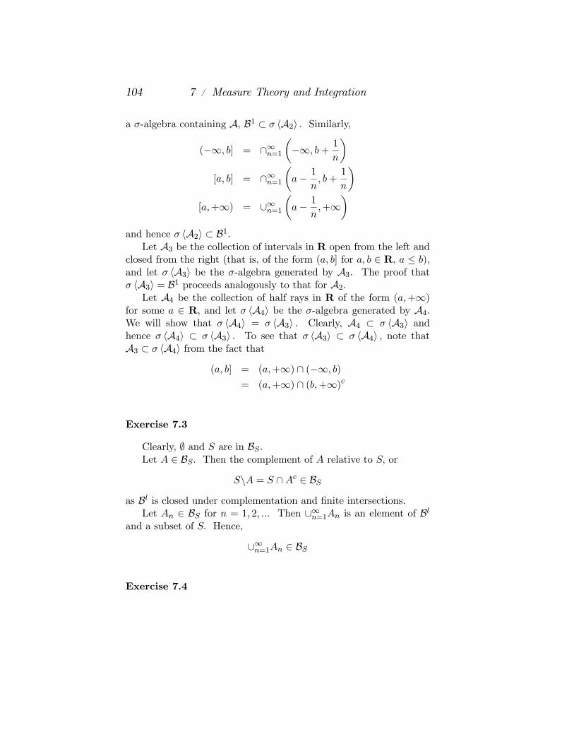
104 7 / Measure Theory and Integration
a σ-algebra containing A, B1 ⊂ σ hA2i . Similarly,
(−∞, b] = ∩∞n=1µ−∞, b+ 1
n
¶[a, b] = ∩∞n=1
µa− 1
n, b+
1
n
¶[a,+∞) = ∪∞n=1
µa− 1
n,+∞
¶and hence σ hA2i ⊂ B1.
Let A3 be the collection of intervals in R open from the left andclosed from the right (that is, of the form (a, b] for a, b ∈ R, a ≤ b),and let σ hA3i be the σ-algebra generated by A3. The proof thatσ hA3i = B1 proceeds analogously to that for A2.
Let A4 be the collection of half rays in R of the form (a,+∞)for some a ∈ R, and let σ hA4i be the σ-algebra generated by A4.We will show that σ hA4i = σ hA3i . Clearly, A4 ⊂ σ hA3i andhence σ hA4i ⊂ σ hA3i . To see that σ hA3i ⊂ σ hA4i , note thatA3 ⊂ σ hA4i from the fact that
(a, b] = (a,+∞) ∩ (−∞, b)= (a,+∞) ∩ (b,+∞)c
Exercise 7.3
Clearly, ∅ and S are in BS.Let A ∈ BS. Then the complement of A relative to S, or
S\A = S ∩Ac ∈ BSas Bl is closed under complementation and finite intersections.
Let An ∈ BS for n = 1, 2, ... Then ∪∞n=1An is an element of Bland a subset of S. Hence,
∪∞n=1An ∈ BS
Exercise 7.4

7 / Measure Theory and Integration 105
We need to establish that the λ in a. and b. are extended realvalued functions satisfying the properties of measures. Typically,these properties are obvious with the possible exception of countableadditivity.
a. Let An∞n=1 be a countable sequence of disjoint subsetsin S. Then
λ (∪∞n=1An) = µ1 (∪∞n=1An) + µ2 (∪∞n=1An)
=∞Xn=1
µ1 (An) +∞Xn=1
µ2 (An)
=∞Xn=1
λ (An) .
b. Let An∞n=1 be a countable sequence of disjoint subsetsin S. Then
λ (∪∞n=1An) = µ1 ((∪∞n=1An) ∩B)= µ1 (∪∞n=1 (An ∩B))
=∞Xn=1
µ1 (An ∩B)
=∞Xn=1
λ (An) ,
where the second inequality comes from the fact that the intersec-tion distributes, and the third equality comes from the fact that theAn ∩B are disjoint.
Exercise 7.5
As A ⊆ B there exists a C = B\A = B ∩ Ac ∈ S such thatA ∪ C = B and A ∩C = ∅. Hence,
µ (A) + µ (C) = µ (B) .

106 7 / Measure Theory and Integration
As µ (C) ≥ 0 we have µ (A) ≤ µ (B) . Further, if µ (A) is finite,µ (B)− µ (A) is well defined and
µ (C) = µ (B\A) = µ (B)− µ (A) .
Exercise 7.6
a. Let A be the family of all complements and finite unionsof intervals of the form (a, b] , (−∞, b] , (a,+∞) , and (−∞,+∞) fora, b ∈ R, a ≤ b. Let C be the collection of sets that can be writtenas a finite disjoint union of such intervals. We follow the Hint andshow that A ⊂ C.
Let A ∈ A. Then by the definition of A, there are three pos-sibilities. If A is an interval of this form, then A ∈ C. If A is afinite union of such intervals, A can always be written as a disjointfinite union of such intervals, and hence A ∈ C. Finally, if A is acomplement of such an interval, note that
(−∞, b]c = (b,+∞)(a, b]c = (−∞, a] ∪ (b,+∞) ∈ C.
Hence A ⊂ C.To show that A is an algebra, note that it obviously contains ∅
and R, and is closed under finite unions. Closure under complemen-tation follows from the fact that, for a, b, c, d ∈ R, a ≤ b ≤ c ≤ d
((a, b] ∪ (c, d])c = (−∞, a] ∪ (b, c] ∪ (d,+∞) ∈ A((−∞, b] ∪ (c, d])c = (b, c] ∪ (d,+∞) ∈ A((a, b] ∪ (c,+∞))c = (−∞, a] ∪ (b, c] ∈ A.
b. We showed in Exercise 7.2 that B1 is the smallest σ-algebracontaining the intervals in R open from the left and closed from theright. Hence, B1 ⊂ σ hAi . To show that σ hAi ⊂ B1, we need toshow that A ⊂ B1. But B1 contains the half-open intervals and isclosed under complementation and finite unions.

7 / Measure Theory and Integration 107
Exercise 7.7
Note: the definition of a measure µ on an algebra A should havespecified that µ is an extended real valued function.
a. Obviously, µ is extended real valued and µ (∅) = 0. LetA ∈ A. Then by Exercise 7.6 a. there exists a finite number ofdisjoint half-open intervals An for n = 1, ..., N such that ∪Nn=1An =A. By property 4,
µ (A) = µ¡∪Nn=1An¢ = NX
n=1
µ (An) ,
which is non-negative as for all n = 1, ..., N the µ (An) are non-negative from properties 2 and 3.
To show countable additivity, let Ai∞i=1 be a countably infinitesequence of disjoint sets in A with ∪∞i=1Ai ≡ A ∈ A. Since A is afinite disjoint union of intervals of the form
(a, b] , (−∞, b] , (a,+∞) , (−∞,+∞)
the sequence Ai can be partitioned into finitely many subsequencessuch that the union of the interavls in each subsequence is a singleinterval of this form. By using such subsequences separately, andusing the finite additivity of µ we may assume that A is of this form.Then
µ (A) = µ (∪ni=1Ai) + µ (A\ ∪ni=1 Ai)
≥ µ (∪ni=1Ai) =nXi=1
µ (Ai) ,
where the equalities comes from finite additivity and the inequalityby non-negativity. Letting n→∞ we get
µ (A) ≥∞Xi=1
µ (Ai) .

108 7 / Measure Theory and Integration
To see the converse, first assume that A = (a, b] for a, b ∈ R.Let ε > 0 and εn∞n=1 be a sequence of real numbers such thatP∞n=1 εn < ε. Renumber the collection of intervals Ai such that
a = a1 < b1 ≤ a2 < ... < bn−1 ≤ an < bn ≤ an+1 < ...,and construct the collection of open intervals Bn such that
B1 = (a1 − ε1, b1 + ε1) ,
and for n ≥ 2Bn = (an, bn + εn) .
Clearly, these intervals form a open covering of the set [a, b] . Butthis set is compact, and hence there exists a finite open subcover,say BnkKk=1 . We may renumber these intervals such thata = an1 ≤ an2 < b1 + ε1 < ... < ank < bnk−1 + εnk−1 ≤ b < bnk + εnk .
Hence
µ ((a, b]) = b− a ≤ (bnK + εnK − an1)
≤KXk=1
[bnk + εnk − ank ]
<KXk=1
[bnk − ank ] + ε
≤∞Xn=1
[bn − an] + ε.
But as ε is arbitrary
µ ((a, b]) = b− a ≤∞Xn=1
µ ((an, bn]) .
To see the result for A of the form (−∞, b] , note that the inter-vals Bn cover [−M, b] for some M finite and hence using the aboveargument
b+M ≤∞Xn=1
µ ((an, bn]) .

7 / Measure Theory and Integration 109
Similarly, for (a,+∞) these intervals cover [a,M ] and we get
M − a ≤∞Xn=1
µ ((an, bn]) .
The desired result follows in each case by letting M →∞.b. As ∅ = (a, a] , we have
µ (∅) =Z a
aπ (s) ds = 0.
Further, as π (s) is non-negative on S, µ (A) is non-negative for allA ∈ A, while, by definition of π
µ (S) =
Z b
aπ (s) ds = 1.
To see countable additivity, let Ai∞i=1 be a countably infinitesequence of disjoint sets in A with ∪∞i=1Ai ≡ A ∈ A. Since A is afinite disjoint union of intervals of the form (c, d] for a ≤ c < d ≤ b,by the same argument as for part a., we can assume A is of the form(c, d] . Note that as π is continuous on [a, b] , it is bounded and hence
µ ((c, d]) =
Z d
cπ (s) ds ≤
Z d
cMds =M (d− c) ,
is bounded for some M <∞.Note first thatZ d
cπ (s) ds = µ ((c, d]) = µ (∪∞i=1Ai)
= µ (∪∞i=1 (ai, bi])= µ (∪ni=1 (ai, bi]) + µ ((c, d] \ ∪ni=1 (ai, bi])
≥ µ (∪ni=1 (ai, bi]) =nXi=1
Z bi
ai
π (s) ds.
Letting n → ∞, and noting that the limit exists in R as this is amontone increasing sequence bounded above, we get
µ ((c, d]) =
Z d
cπ (s) ds ≥
∞Xi=1
Z bi
ai
π (s) ds.

110 7 / Measure Theory and Integration
To see the converse, let ε > 0 and εn∞n=1 be a sequence of realnumbers such that
∞Xn=1
Z bnk+εnk
bnk
π (s) ds < ε.
Renumber the collection of intervals Ai = (ai, bi] such that
c = a1 < b1 ≤ a2 < ... < bn−1 ≤ an < bn ≤ an+1 < ... ≤ d,and construct the collection of open intervals Bn such that
B1 = (a1 − ε1, b1 + ε1) ,
and for n ≥ 2Bn = (an, bn + εn) .
Clearly, these intervals form a open covering of the set [c, d] . Butthis set is compact, and hence there exists a finite open subcover,say BnkKk=1 . We may renumber these intervals such thata = an1 ≤ an2 < b1 + ε1 < ... < ank < bnk−1 + εnk−1 ≤ b < bnk + εnk .
Hence
µ ((c, d]) =
Z d
cπ (s) ds
≤Z bnK+εnK
an1
π (s) ds
≤KXk=1
Z bnk+εnk
ank
π (s) ds
=KXk=1
Z bnk
ank
π (s) ds+KXk=1
Z bnk+εnk
bnk
π (s) ds
<KXk=1
Z bnk
ank
π (s) ds+ ε
≤∞Xn=1
Z bn
an
π (s) ds+ ε.

7 / Measure Theory and Integration 111
But as ε is arbitrary
µ ((c, d]) =
Z d
cπ (s) ds ≤
∞Xn=1
µ ((an, bn]) =∞Xn=1
Z bn
an
π (s) ds.
Exercise 7.8
Clearly, S 0 contains ∅ and S. To see closure under complemen-tation, let A0 ∈ S 0. Then there exists A ∈ S, C1, C2 ∈ C such that
A0 = (A ∪C1) \C2.Hence
A0c = (Ac ∩Cc1) ∪ C2= (Ac ∪C2) \ (C1\C2) ,
which is in S 0.To see closure under countable unions, for all n = 1, 2, ... let
A0n ∈ S 0. Then for each n there exists an An ∈ S and C1n, C2n ∈ Csuch that
A0n = (An ∪C1n) \C2n.Define A0 = ∪∞n=1A0n, A = ∪∞n=1An, C1 = ∪∞n=1C1n, and C2 =∪∞n=1C2n. Then
(A ∪ C1) \C2 ⊆ A0 ⊆ A0 = A ∪ C1,and
µ ((A ∪ C1) \C2) = µ (A ∪ C1) .Hence, there exists a C 02 ∈ C such that A0 = (A ∪ C1) \C 02. Hence,A0 ∈ S 0.
Exercise 7.9
a. The definitions differ as to whether the “ ≤ ” ins ∈ S : f (s) ≤ a ∈ S, all a ∈ R (1)

112 7 / Measure Theory and Integration
is replaced with≥, < or> . Proof of equivalence requires establishingthat (1) is equivalent to the equivalent statement sets defined by ≥,< or > .
≤⇔>: Follows from the fact that, for all a ∈ Rs ∈ S : f (s) ≤ a ∈ S ⇐⇒ s ∈ S : f (s) ≤ ac ∈ S
⇐⇒ s ∈ S : f (s) > a ∈ Sas S is closed under complementation.
≥ ⇔ <: Follows analogously.
≤ ⇒ <: for any a ∈ R, for n ≥ 1 consider the sequence of setsAn =
©s ∈ S : f (s) ≤ a− 1
n
ªwhich are in S by (1). Then
A ≡ s ∈ S : f (s) < a = ∪∞n=1Anis in S by closure under countable unions.
≤ ⇐= <: for any a ∈ R, for n ≥ 1 consider the sequence of setsAn =
©s ∈ S : f (s) < a+ 1
n
ªin S. Then
A ≡ s ∈ S : f (s) ≤ a = ∩∞n=1Anis in S by closure under countable intersections.
b. Assume that s ∈ S : f (s) ≤ a ∈ S for all a ∈ R. Thenby the result of part a., for all a ∈ R s ∈ S : f (s) ≥ a ∈ S. Hences ∈ S : f (s) = a = s ∈ S : f (s) ≥ a ∩ s ∈ S : f (s) ≤ a ∈ Sfor all a ∈ R by closure under finite intersections.
To show that the converse is false, as a counterexample let S =(0, 1] and let S be the set of all countable and co-countable subsets ofS (where a co-countable set is a set with a countable complement).It is easily verified that S is a σ-algebra. Consider the functionf (s) = s. Then the set
s ∈ S : f (s) = a =½ ∅ a /∈ (0, 1]a a ∈ (0, 1]

7 / Measure Theory and Integration 113
The empty set is finite and hence countable. Hence these sets arein S. However, the set s ∈ S : f (s) ≤ a for any a ∈ (0, 1) is equalto (0, a] which is neither countable or co-countable.
c. The sets
A ≡ s ∈ S : f (s) = −∞ = ∩∞n=1 s ∈ S : f (s) < −nB ≡ s ∈ S : f (s) = +∞ = ∩∞n=1 s ∈ S : f (s) > n
are in S because S is closed under countable intersections.
Exercise 7.10
a. Let f be monotone increasing. Then for some a ∈ R theset
s ∈ R : f (s) ≤ ais either of the form s ∈ R : s ≤ a or s ∈ R : s < a . Both are inB by Exercise 7.6. The proof for monotone decreasing f is analogous.
Let f be continuous. By Exercise 7.9 a. it is sufficient to showthat for all a ∈ R the set s ∈ R : f (s) < a is in B. But as f iscontinuous, this set is open and hence in B.
b. For any f : S → R the set s ∈ S : f (s) ≤ a is a subsetof S and is hence in S. Hence, all functions are measurable.
Exercise 7.11
Let Ai ∈ S, i = 1, ..., n and without loss of generality, reorderi = 1, ..., n such that a1 < a2 < ... < an which is possible as the aiare distinct. Then for all a ∈ R, the set
s ∈ S : φ (s) ≥ a
is either ∅ ∈ S if a > an, S ∈ S if a ≤ a1, or, for j = 2, ..., nBj = ∪nk=jAk if aj−1 < a ≤ aj . As S is closed under finite unions,Bj ∈ S for j = 2, ..., n and hence φ is measurable.

114 7 / Measure Theory and Integration
Let φ be measurable. Without loss of generality, reorder i =1, ..., n such that a1 < a2 < ... < an. Then for all a ∈ R
s ∈ S : φ (s) ≥ a ∈ S
and hence s ∈ S : φ (s) < a ∈ S as S is closed under complemen-tation. For all i there exist bi, ci ∈ R such that ai−1 < bi < ai <ci < ai+1. Then
Ai = s ∈ S : φ (s) ≥ bi ∩ s ∈ S : φ (s) < ci ∈ S
as S is closed under finite intersections.
Exercise 7.12
a. Let f and g be measurable functions and c ∈ R. ByTheorem 7.5 there exists sequences of measurable simple functionsfn and gn such that fn → f and gn → g pointwise. In eachcase we will exhibit a sequence of measurable simple functions thatconverges pointwise to the desired function. The result will thenfollow by Theorem 7.4.
f+g : Let hn ≡ fn+gn which converges pointwise to h ≡ f+gbecause for any sequences of real numbers xn and yn we knowxn+yn → x+y. To see that each hn is a measurable simple function,note that it can take on at most a finite number of values on a finitenumber of sets, all of which are measurable by the fact that S isclosed under finite intersections and set differences.
fg : Let hn ≡ fngn which converges pointwise to h ≡ fgbecause for any sequences of real numbers xn and yn we knowxnyn → xy. That the hn’s are measurable simple functions followsfrom the fact that each hn is non-zero only if both fn and gn arenon-zero. This can happen on only a finite number of sets, all ofwhich are measurable as S is closed under finite intersections.
|f | : Let hn ≡ |fn| = f+n − f−n which converges pointwiseto h ≡ |f | because for any sequence of real numbers xn we know

7 / Measure Theory and Integration 115
−xn → −x. The hn are measurable simple functions, for ifPNni=1 aiχAn
is the standard representation of fn, thenPNni=1 |ai|χAn is the stan-
dard representation of hn.
cf : Let hn ≡ cfn which obviously converges pointwise toh ≡ cf. The hn are measurable simple functions with standardrepresentation
PNni=1 caiχAn (s) .
b. To show that supn fn is measurable, we need to show thatfor all a ∈ R ½
s ∈ S : supnfn ≤ a
¾∈ S
As for all n = 1, 2, ... the fn are measurable, s ∈ S : fn ≤ a ∈ S forall n. But ½
s ∈ S : supnfn ≤ a
¾= ∩∞n=1 s ∈ S : fn ≤ a
which is measurable because S is closed under countable intersec-tions.
That infn fn is measurable comes from
infnfn = − sup
n(−fn)
which is measurable by part a. and the fact that supn fn is measur-able. Similarly, noting that
lim inf fn = supm≥1
µinfn≥m
fn
¶lim sup fn = inf
m≥1
µsupn≥m
fn
¶we can iterate on the above results to get that lim inf fn and lim sup fnare measurable.
Exercise 7.13

116 7 / Measure Theory and Integration
a. By the result of Exercise 7.9 a. a continuous function fon Rl will be Bl-measurable if, for all a ∈ Rn
x ∈ Rl : f (x) < ao∈ Bl
But the set (−∞, a) is open in R, and as f is continuousnx ∈ Rl : f (x) < a
ois open and is hence an element of Bl.
Note: In answering part b., we will follow Billingsley (1995,pp. 183-186) in defining the Baire functions to be real valued func-tions (as opposed to extended real valued).
b. Let X be the smallest class of real valued functions onRl containing the continuous functions and closed under pointwisepassages to the limit that do not give rise to ±∞. That is, if fn is asequence of real valued functions in X converging pointwise to f, andif f is real valued, then f ∈ X . Let Y denote the Borel measurablereal valued functions on Rl.
X ⊂ Y : Note that the argument of Exercise 7.10 a. extendsto continuous real valued functions on Rl. Hence, all continuous realvalued functions are in Y. Further, by Exercise 7.12 b., Y is closedunder pointwise passages to the limit that do not give rise to ±∞.As X is the smallest such class of functions, X ⊂ Y.
Y ⊂ X : The argument proceeds in the following four steps.First, note that if f, g ∈ X and a, b ∈ R, by the result of Exercise7.12 (which applies because X ⊂ Y), max f, g ∈ X (where themaximum is pointwise) and af + bg ∈ X .
Second, let A = ©A ⊂ Rl : χA ∈ Xª . We will use the first resultto show that this is a σ-algebra. Note that as χRl is continuous,Rl ⊂ A. To show closure under complementation, let A ∈ A. Then
χAc = χRl − χA

7 / Measure Theory and Integration 117
which is in X by the first result. To show closure under comple-mentation, for n ≥ 1, let An ∈ A. To show that ∪∈n=1An ∈ A,let
f1 = χA1
fn = maxnfn,χAn−1
owhere the first is in X by assumption, and the second by the firstresult. Therefore,
χA = limn→∞ fn
which is in X .Third, for x ∈ Rl note that
C =ns ∈ Rl : sn ≤ xn, n = 1, ..., l
o∈ A.
To see this, define for i = 1, ..., l
Ci =ns ∈ Rl : si ≤ xi
ogi (s) =
1 if s ∈ Ci
xi + 1− si if si ∈ [xi, xi + 1]0 if si > xi + 1
As the gi are continuous, and as
χC = −max −g1,−g2, ...,−glby the first result above, C ∈ A. Hence, as A is a σ-algebra contain-ing the sets of the form C, which generate Bl, we have Bl ⊂ A.
Finally, by Theorem 7.5 all Borel functions can be written as thepointwise limit of a sequence of Borel simple functions that do notgive rise to ±∞. But as Bl ⊂ A, the indicator functions of Borel setsare in X . Further, by the first result, finite combinations of indicatorfunctions are in X , and hence X includes all Borel simple functions.Hence, as X is closed under pointwise passages to the limit that donot give rise to ±∞, Y ⊂ X .
Exercise 7.14

118 7 / Measure Theory and Integration
Denote f−1 (A) = x ∈ S : f (x) ∈ A and let
G = ©A ⊂ R : f−1 (A) ∈ Sª .We will show that G is a σ-algebra containing the open intervals inR, and hence that B ⊂ G.
G is a σ-algebra, from the fact that f−1 (R) = S, the fact that¡f−1 (A)
¢c= x ∈ S : f (x) ∈ Ac= x ∈ S : f (x) ∈ Ac= f−1 (Ac) ,
and that
f−1 (∪∞n=1An) = x ∈ S : f (x) ∈ ∪∞n=1An= ∪∞n=1 x ∈ S : f (x) ∈ An= ∪∞n=1f−1 (An) .
By definition of f measurable and Exercise 7.9, G contains the openintervals.
Exercise 7.15
Suppose fi for i = 1, ...,m is Bl-measurable. Then for all i =1, ...,m, for all ai, bi ∈ R, ai ≤ bi
Ai ≡ns ∈ Rl : fi (s) ∈ (ai, bi)
o∈ Bl
Let B = s ∈ Rm : si ∈ (ai, bi) , i = 1, ...,m . Thenns ∈ Rl : f (s) ∈ B
o= ∩mi=1Ai ∈ Bl
Now suppose that f is measurable, and for all i = 1, ...,m, for allai, bi ∈ R, ai ≤ bi let
Bi (ai, bi) = s ∈ Rm : si ∈ (ai, bi) , i = 1, ...,m

7 / Measure Theory and Integration 119
Thenns ∈ Rl : f (s) ∈ Bi (ai, bi)
o=ns ∈ Rl : fi (s) ∈ (ai, bi)
o∈ Bl
and fi is Bl-measurable
Exercise 7.16
Consider any finite partition of [0, 1] into intervals of the form[ai−1, ai] for i = 1, ..., n. As each interval contains both rational andirrational numbers, if we choose the yi ≤ f (x) , all x ∈ [ai−1, ai] , thesum
Pni=1 yi (ai − ai−1) ≤ 0. Moreover, we can always choose the yi
so that this sum is equal to zero. Hence, the supremum over all suchpartitions, which is the lower Reimann integral, is zero. Similarly, ifwe choose yi ≥ f (x) , all x ∈ [ai−1, ai] the sum
Pni=1 yi (ai − ai−1) ≥
1, and the yi can be chosen so that this sum equals one. Hence,the infimum over all such partitions, which is the upper Riemannintegral, is one. As they are not equal, the function is not Riemannintegrable.
Exercise 7.17
Let φ and ψ have standard representations
φ (s) =
n1Xi=1
aiχAi (s)
ψ (s) =
n2Xj=1
bjχBj (s)
Then φ+ ψ has a representation
(φ+ ψ) (s) =
n1Xi=1
n2Xj=1
(ai + bj)χAi∩Bj (s)
where the sets Ai ∩ Bj are disjoint from the fact that the Ai andBj are separately disjoint. However, this need not be the standard

120 7 / Measure Theory and Integration
representation of φ + ψ as the ai + bj need not be distinct. Letk = 1, ...,K index the distinct numbers ck in the set
ai + bj : i = 1, ..., n1, j = 1, ..., n2and denote by k the collection of indices (i, j) that deliver thisnumber
k = (i, j) , i = 1, ..., n1, j = 1, ..., n2 : ai + bj = ck .Define Ck as the union over all sets Ai ∩ Bj such that ai + bj = ck,so that
µ (Ck) =Xkµ (Ai ∩Bj) .
Then the standard representation of φ+ ψ is given by
(φ+ ψ) (s) =KXk=1
ckχCk .
ThenZ(φ+ ψ) dµ =
KXk=1
ckµ (Ck)
=KXk=1
Xkckµ (Ai ∩Bj)
=KXk=1
Xk(ai + bj)µ (Ai ∩Bj)
=
n1Xi=1
n2Xj=1
(ai + bj)µ (Ai ∩Bj)
=
n1Xi=1
n2Xj=1
aiµ (Ai ∩Bj) +n1Xi=1
n2Xj=1
bjµ (Ai ∩Bj)
=
n1Xi=1
aiµ (Ai) +
n2Xj=1
bjµ (Bj)
=
Zφdµ+
Zψdµ

7 / Measure Theory and Integration 121
where the second last equality follows from the fact that
µ (Ai) =
n2Xj=1
µ (Ai ∩Bj)
µ (Bj) =
n1Xi=1
µ (Ai ∩Bj) .
If c = 0, then cφ vanishes indentically and the equality holds. Ifc > 0, then cφ has standard representation
n1Xi=1
caiχAi
Therefore,Zcφdµ =
n1Xi=1
caiµ (Ai) = c
n1Xi=1
aiµ (Ai) = c
Zφdµ.
Exercise 7.18
a. By definitionZfdµ = sup
Zφdµ,
where the sup is over all simple functions φ in M+ (S,S) with 0 ≤φ ≤ f. As f ≤ g, the subset of simple functions φ in M+ (S,S)satisfying 0 ≤ φ ≤ g is at least as large as that for f. Hence,Z
fdµ ≤Zgdµ.
b. Note that ZAfdµ =
ZfχAdµ,Z
Bfdµ =
ZfχBdµ.

122 7 / Measure Theory and Integration
As A ⊆ B we have that fχA ≤ fχB and hence by the result of parta. Z
Afdµ ≤
ZBfdµ.
Exercise 7.19
Consider the constant function f : S → R+ defined by f (s) =a ≥ 1 for all s ∈ S, and for all n = 1, 2, ..., let fn (s) = a−1/n. Thenfn is a monotone increasing sequence of functions inM+ (S,S) . Letα = 1 and consider the simple function ϕ (s) = f (s) which satisfies0 ≤ ϕ ≤ f. Then
An = s ∈ S:fn (s) ≥ αϕ (s)= s ∈ S:fn (s) ≥ f (s) = ∅
for all n. Hence, ∪∞n=1An = ∅ 6= S.
Exercise 7.20
a. Let f, g ∈ M+ (S,S) . By Theorem 7.5 there exists se-quences of non-negative simple functions fn and gn such that
0 ≤ f1 ≤ ... ≤ fn ≤ ... ≤ f for all n,0 ≤ g1 ≤ ... ≤ gn ≤ ... ≤ g for all n,
Then for all n = 1, 2, ..., the function sn ≡ fn + gn is a non-negativesimple function satisfying
0 ≤ s1 ≤ ... ≤ sn ≤ ... ≤ s ≡ f + g for all n.
Hence, Zsdµ = lim
n→∞
Zsndµ
= limn→∞
Zfndµ+ lim
n→∞
Zgndµ
=
Zfdµ+
Zgdµ,
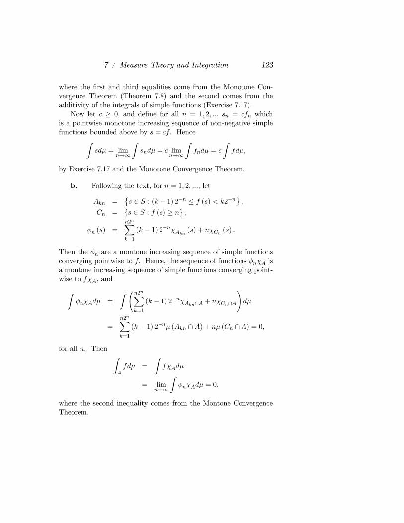
7 / Measure Theory and Integration 123
where the first and third equalities come from the Monotone Con-vergence Theorem (Theorem 7.8) and the second comes from theadditivity of the integrals of simple functions (Exercise 7.17).
Now let c ≥ 0, and define for all n = 1, 2, ... sn = cfn whichis a pointwise monotone increasing sequence of non-negative simplefunctions bounded above by s = cf. HenceZ
sdµ = limn→∞
Zsndµ = c lim
n→∞
Zfndµ = c
Zfdµ,
by Exercise 7.17 and the Monotone Convergence Theorem.
b. Following the text, for n = 1, 2, ..., let
Akn =©s ∈ S : (k − 1) 2−n ≤ f (s) < k2−nª ,
Cn = s ∈ S : f (s) ≥ n ,
φn (s) =n2nXk=1
(k − 1) 2−nχAkn (s) + nχCn (s) .
Then the φn are a montone increasing sequence of simple functionsconverging pointwise to f. Hence, the sequence of functions φnχA isa montone increasing sequence of simple functions converging point-wise to fχA, andZ
φnχAdµ =
Z Ãn2nXk=1
(k − 1) 2−nχAkn∩A + nχCn∩A!dµ
=n2nXk=1
(k − 1) 2−nµ (Akn ∩A) + nµ (Cn ∩A) = 0,
for all n. Then ZAfdµ =
ZfχAdµ
= limn→∞
ZφnχAdµ = 0,
where the second inequality comes from the Montone ConvergenceTheorem.

124 7 / Measure Theory and Integration
c. Note that f ≥ f∗ ≡ ∞χA. Hence, by Exercise 7.18a.
∞ >
Zfdµ ≥
Zf∗dµ =∞µ (A) ,
which implies µ (A) = 0.
Exercise 7.21
Defined this way, λ is clearly non-negative and satisfies λ (∅) = 0.To see countable additivity, let Ai i ≥ 1 be a sequence of disjointsets in S with A = ∪∞i=1Ai. For n ≥ 1, let fn =
Pni=1 fχAi. Then
by Exercise 7.20a. we haveZfndµ =
nXi=1
ZfχAidµ =
nXi=1
λ (Ai) .
As fn is a monotone increasing sequence of non-negative functionsconverging pointwise to fχAi , the above result and the MonotoneConvergence Theorem (Theorem 7.8) imply that
λ (A) =
ZfχA.dµ = lim
n→∞
Zfndµ
=∞Xi=1
λ (Ai) .
Exercise 7.22
As the gi are non-negative, the sequence fn defined by fn =Pni=1 gi, n = 1, 2, ..., is non-decreasing and converges pointwise to
f =P∞i=1 gi. By Exercise 7.20, we haveZ
fndµ =
Z nXi=1
gidµ =nXi=1
Zgidµ,

7 / Measure Theory and Integration 125
and taking limits gives
limn→∞
Z nXi=1
gidµ = limn→∞
nXi=1
Zgidµ.
But, by the Monotone Convergence Theorem (Theorem 7.8)
limn→∞
Z nXi=1
gidµ = limn→∞
Zfndµ =
Zfdµ =
Z ∞Xi=1
gidµ,
and the result follows.
Exercise 7.23
Let S = (0, 1] , S = B(0,1], µ the Lebesgue measure and considerthe sequence of functions for n = 1, 2, ...
fn = nχ(0,1/n].
As infn fn ≥ 0 Fatou’s Lemma applies. Noting that lim infn fn = 0and
Rfndµ = 1 for all n we have
0 =
Zlim inf
nfndµ < lim inf
n
Zfndµ = 1.
Exercise 7.24
a. For f ∈M+ the sequence of sets Bn ≡©s ∈ S : f (s) ≥ 1
n
ªand the sequences of functions fn ≡ fχBn satisfy
B1 ⊆ B2 ⊆ ... ⊆ Bn ⊆ ... ⊆ B ≡ s ∈ S : f (s) > 0 ,
andf1 ≤ f2 ≤ ... ≤ fn ≤ ... ≤ f = fχB.
Then Zfdµ = 0⇒
Zfndµ = 0,

126 7 / Measure Theory and Integration
for all n = 1, 2, ... asRfndµ converges to
Rfdµ = 0 from below by
the Monotone Convergence Theorem (Theorem 7.8). This impliesthat µ (Bn) = 0 from the fact that
0 ≤ 1
nχBn ≤ fn,
and so
0 ≤ 1
nµ (Bn) ≤
Zfndµ.
But this implies that µ (B) = 0 by Theorem 7.1a.Now suppose that µ (B) = 0. Then for all n = 1, 2, ... we must
have µ (Bn) = 0. Noting that
fn ≤ ∞χBn .
Exercise 7.18a. gives
0 ≤Zfndµ ≤ ∞µ (Bn) ,
from which we get thatRfndµ = 0. The result follows from the
Monotone Convergence Theorem.
b. Let fn be a monotone increasing sequence of functionsin M+ that converges to f µ-almost everywhere and let f∗ be thepointwise limit of this sequence. By Theorem 7.4 f∗ is measurable,and by the Monotone Convergence Theorem (Theorem 7.8) we have
limn→∞
Zfndµ =
Zf∗dµ.
We know that µ (s ∈ S : f (s) 6= f∗ (s)) = 0. Therefore, by part a.Z(f − f∗) dµ = 0,
and hence by Exercise 7.20 a. we getZfdµ =
Zf∗dµ.

7 / Measure Theory and Integration 127
Exercise 7.25
If f is bounded, there exists a B ∈ R such that for all s ∈ S wehave |f | (s) ≤ B. HenceZ
f+dµ ≤ Bµ (S) <∞,
and Zf−dµ ≤ Bµ (S) <∞.
Exercise 7.26
a. Note that |f | = f+ + f− and hence that |f |+ = f+ + f−while |f |− = 0. If f is µ-integrable, then f+ and f− have finiteintegrals with respect to µ and hence so does |f |+. Therefore, |f | isintegrable. If |f | is integrable, |f |+ has a finite integral with respectto µ and hence so must f+ and f−. Finally,¯Z
fdµ
¯=
¯Zf+dµ−
Zf−dµ
¯≤
Zf+dµ+
Zf−dµ =
Z|f | dµ.
b. Note that
f+ + f− = |f | ≤ |g| = g+ + g−.Hence by Exercise 7.18 a.Z
f+dµ ≤Z|g| dµ <∞,
and Zf−dµ ≤
Z|g| dµ <∞,
which implies that |f | is µ-integrable, and moreoverZ|f | dµ ≤
Z|g| dµ <∞,
128 7 / Measure Theory and Integration
by Exercise 7.18a.
c. Let α ∈ [0,+∞) . Then (αf)+ = αf+ and (αf)− = αf−.Hence,
Rαf+dµ = α
Rf+dµ < ∞ and
Rαf−dµ = α
Rf−dµ < ∞
by Exercise 7.20. Hence, αf is integrable andZαfdµ =
Zαf+dµ−
Zαf−dµ = α
Zfdµ.
Now let α ∈ (−∞, 0] . Then (αf)+ = −αf− and (αf)− = −αf+.Integrability follows as above, and henceZ
αfdµ =
Z−αf−dµ−
Z−αf+dµ
= α
Z ¡f+ − f−¢ dµ = α
Zfdµ.
Note that (f + g)+ ≤ f+ + g+ and (f + g)− ≤ f− + g−. Thenas f and g are integrable, by Exercise 7.20 f + g is integrable. Thenas
(f + g)+ − (f + g)− = f + g = ¡f+ − f−¢+ ¡g+ − g−¢ ,we get
(f + g)+ + f− + g− = (f + g)− + f+ + g+.
By Exercise 7.20 Z(f + g)+ dµ+
Zf−dµ+
Zg−dµ
=
Z(f + g)− dµ+
Zf+dµ+
Zg+dµ.
Subtracting the finite numbersRf−dµ,
Rg−dµ, and
R(f + g)− dµ
from both sides givesZ(f + g) dµ =
Z(f + g)+ dµ−
Z(f + g)− dµ
=
Zf+dµ−
Zf−dµ+
Zg+dµ−
Zg−dµ
=
Zfdµ+
Zgdµ.

7 / Measure Theory and Integration 129
Exercise 7.27
Let F be the set of all finite unions of disjoint measurable rectan-gles, and let G be the algebra generated by the measurable rectangles.We will show that E = F = G.
Obviously, F ⊂ E ⊂ G. The proof will be complete if we canestablish that G ⊂ F . But F contains the measurable rectangles,and so we only need to show that it is an algebra.
∅, X × Y ∈ F : ∅ and X × Y are measurable rectangles.
To establish closure under complementation, we will first estab-lish that F is closed under finite intersections. First, let B and C ∈F . Therefore there exist BnNn=1 and CmMm=1 sequences of disjointmeasurable rectangles such that ∪Nn=1Bn = B and ∪Mm=1Cm = C.Then
B ∩ C =¡∪Nn=1Bn¢ ∩ ¡∪Mm=1Cm¢
=¡∪Nn=1B1n ×B2n¢ ∩ ¡∪Mm=1C1m × C2m¢
= ∪Nn=1 ∪Mm=1 (B1n ×B2n) ∩ (C1m × C2m)= ∪Nn=1 ∪Mm=1 (B1n ∩ C1m)× (B2n ∩C2m) ,
which is a finite unions of disjoint measurable rectangles. Iteratingon this gives us the result for arbitrary finite unions.
A ∈ F ⇒ Ac ∈ F : Let A ∈ F . Then there exists AnNn=1disjoint measurable rectangles such that ∪Nn=1An = A and Ac =∩Nn=1Acn. For any measurable rectangle An = XA × YA, Acn canbe written as the union of three measurable rectangles (Xc
A × YA) ,(XA × Y cA), and (Xc
A × Y cA) . To see this note that if (x, y) ∈ Acn,then either x /∈ XA, or y /∈ YA, or both. Hence, (x, y) is an elementof one of these rectangles. The reverse is obvious.
But these rectangles are also disjoint. Hence, the result followsby closure under finite intersections.
To establish closure under finite unions, we first establish closureunder finite differences. If A,B ∈ F they can be written as A =

130 7 / Measure Theory and Integration
∪Nn=1An and B = ∪Mm=1Bm for finite disjoint collections of C setsAn and Bm . Then
A\B =¡∪Nn=1An¢ ∩ ¡∪Mm=1Bm¢c
=¡∪Nn=1An¢ ∩ ¡∩Mm=1Bcm¢
= ∪Nn=1¡∩Mm=1 (An\Bm)¢ .
Writing An = Xn×Yn and Bm = Um×Vm, we have that for all n,m,An\Bm is the union of the disjoint measurable rectangles (Xn\Um)×Yn and (Xn ∩ Um) × (Yn\Vm) . But we saw above that F is closedunder finite intersections, and hence A\B is a finite union of disjointmeasurable rectangles.
An ∈ F , n = 1, ..., N ⇒∪Nn=1An ∈ F :We demonstrate the resultfor N = 2. Iterating on the argument gives the result for arbitraryfinite N. Note that
A1 ∪A2 = (A1\A2) ∪ (A2\A1) ∪ (A1 ∩A2)
is a finite union of disjoint measurable rectangles using the factsproven above that F is closed under finite set differences and finiteintersections.
Exercise 7.28
It is sufficient to show that each σ-algebra contains the generatorsof the other.
Bk+l ⊂ Bk × Bl : Bk+l is generated by A, the collection of setsof the form
A =nx ∈ Rk+l : xi ∈ (ai, bi) , i = 1, ..., k + l
o.
We will refer to these sets as the measurable pavings in Rk+l. Butsuch pavings are measurable rectangles and are in E . Hence Bk×Blis a σ-algebra containing A and Bk+l ⊂ Bk × Bl.

7 / Measure Theory and Integration 131
Bk+l ⊃ Bk × Bl : The text defines Bk × Bl as the σ-algebragenerated by E ; it is easily seen that it is also the σ-algebra generatedby C. It is sufficient to show that C ⊂ Bk+l. That is, if B ∈ Bk andC ∈ Bl, B × C ∈ Bk+l.
Let B be a measurable paving in Rk and consider the class
M =nC ⊂ Rl : B × C ∈ Bk+l
o.
It is easily verified thatM is a σ-algebra, and as Bk+l contains themeasurable pavings inRk+l,Mmust contain the measurable pavingsin Rl. Hence Bl ⊂M.
Now fix C ∈ Bl and consider the class of sets
N =nB ⊂ Rk : B × C ∈ Bk+l
o.
This is a σ-algebra, and by the result immediately above containsthe measurable pavings in Rk. Hence Bk ⊂ N .
From this, if B ∈ Bk and C ∈ Bl, B × C ∈ Bk+l and Bk+l ⊃Bk × Bl.
Exercise 7.29
Let E ∈ E . If we can show that E can be written as a finite unionof disjoint measurable rectangles (that is, if we can adapt Exercise7.27 to this set-up), we can use the argument in the proof of Theorem7.13 to show that we can extend µ to E . The extension to Z willthen follow from the Hahn and Caratheodory Extension Theorems.
Let F be the set of all finite unions of disjoint measurable rectan-gles. Once again we only need to show that it is an algebra. Thatit contains ∅ and Z is immediate. To show closure under comple-mentation and finite unions, we first establish that F is closed underfinite intersections and finite differences.
To establish closure under finite intersections, first let B and C ∈F . Therefore there exist BkKk=1 and CmMm=1 sequences of disjoint

132 7 / Measure Theory and Integration
measurable rectangles such that ∪Kk=1Bk = B and ∪Mm=1Cm = C.Then B ∩C equals¡∪Kk=1Bk¢ ∩ ¡∪Mm=1Cm¢=
¡∪Kk=1B1k ×B2k × ...×Bnk¢ ∩ ¡∪Mm=1C1m × C2m × ...× Cnm¢= ∪Kk=1 ∪Mm=1 (B1k ∩ C1m)× (B2k ∩ C2m)× ...× (Bnk ∩ Cnm) ,
which is a finite unions of disjoint measurable rectangles.To establish closure under finite differences, let A,B ∈ F . Hence
they can be written as A = ∪Kk=1An and B = ∪Mm=1Bm for finitedisjoint collections of C sets An and Bm . Then
A\B =¡∪Kk=1Ak¢ ∩ ¡∪Mm=1Bm¢c
=¡∪Kk=1Ak¢ ∩ ¡∩Mm=1Bcm¢
= ∪Kk=1¡∩Mm=1 (Ak\Bm)¢ .
But we saw above that F is closed under finite intersections. HenceA\B will be a finite union of disjoint measurable rectangles if we canprove that for all k,m, Ak\Bm is a finite union of disjoint measurablerectangles. The proof of this is constructive. Writing Ak = X1Ak ×X2Ak × ... ×XnAk and Bm = X1Bm ×X2Bm × ... ×XnAm , we havethat
Ak = X1Ak ×X2Ak × ...×XnAk= ((X1Ak\X1Bm) ∪ (X1Ak ∩X1Bm))×X2Ak × ...×XnAk= [(X1Ak\X1Bm)×X2Ak × ...×XnAk ] ∪
[(X1Ak ∩X1Bm)×X2Ak × ...×XnAk ]= [(X1Ak\X1Bm)×X2Ak × ...×XnAk ] ∪
[(X1Ak ∩X1Bm)× (X2Ak\X2Bm)× ...×XnAk ] ∪[(X1Ak ∩X1Bm)× (X2Ak ∩X2Bm)× ...×XnAk ] .
Iterating on this process gives the result.We can now prove closure under complementation and finite
unions.
A ∈ F ⇒ Ac ∈ F : Let A ∈ F . Then there exists AkKk=1 dis-joint measurable rectangles such that ∪Kk=1Ak = A andAc = ∩Kk=1Ack.

7 / Measure Theory and Integration 133
For any measurable rectangle Ak = X1Ak × X2Ak × ... × XnAk , Ackcan be written as the union of disjoint measurable rectangles con-structed the following way. For j = 0, ..., n − 1, let Aj repre-sent the collection of measurable rectangles constructed from prod-ucts of the XmAk ’s with exactly j of the X
cmAk
’s. Thus, A0 =nXc1Ak
×Xc2Ak
× ...×XcnAk
o. Then taking the union of all the ele-
ments of these collections for j = 0, ..., n−1 gives us Ack ∈ F . Hence,the result follows by closure under finite intersections.
An ∈ F , n = 1, ...,N ⇒∪Nn=1An ∈ F :We demonstrate the resultfor N = 2. Iterating on the argument gives the result for arbitraryfinite N. Note that
A1 ∪A2 = (A1\A2) ∪ (A2\A1) ∪ (A1 ∩A2)
is a finite union of disjoint measurable rectangles using the factsproven above that F is closed under finite set differences and finiteintersections.
Exercise 7.30
Let E be a subset of R that is not Lebesgue measurable, and letF ∈ L1 be such that λ (F ) = 0. Then the set E × F is a subset ofR× F and has Lebesgue measure zero. Hence, E × F ∈ L2.
Exercise 7.31
We need to show that for all A ∈ S,
φ−1 (A) ≡ (w,x) ∈W ×X : φ (w, x) ∈ A ,
is an element of W ×X . Define the function b : W × X → Y × Zby b (w, x) = (f (x) , g (y)) . Then we can write φ = h b. Theproof will be complete if we can show that b is measurable betweenW ×X and Y ×Z, and that compositions of measurable functionsare measurable.

134 7 / Measure Theory and Integration
To see that compositions of measurable functions are measurablein general, let (Ω,F) , (Ω0,F 0) and (Ω00,F 00) be measurable spaces,and let T : Ω→ Ω0 be measurable between F and F 0, and T 0 : Ω0 →Ω00 be measurable between F 0 and F 00. Then T 0 T : Ω → Ω00 ismeasurable between F and F 00 because, if A00 ∈ F 00, then¡
T 0 T¢−1 ¡A00¢ = T−1 ³¡T 0¢−1 ¡A00¢´ ∈ F ,because (T 0)−1 (A00) ∈ F 0 as T 0 is measurable, and T is measurable.
To see that b is measurable between W ×X and Y ×Z, we firstestablish that if E is a measurable rectangle in Y ×Z, then b−1 (E)is a measurable rectangle in W ×X . We then show that the set ofall subsets in Y × Z with inverse images in W ×X , call it G, is aσ-algebra. Then by construction, we will have Y ×Z ⊂ G and theresult will be proven.
Let E be a measurable rectangle in Y ×Z. Then b−1 (E) isa measurable rectangle in W ×X because f and g are measurable.Now define
G = ©B ⊂ Y × Z : b−1 (B) ∈W ×Xª .But G contains the measurable rectangles in W ×X , and is a σ-algebra. To see the latter, note first that
b−1 (Y × Z) =W ×X.Also, if B ∈ G, then as
b−1 (Bc) =¡b−1 (B)
¢c,
we must have Bc ∈ G. Finally, if Bn∞n=1 is in G, then ∪∞n=1Bn ∈ Gas
b−1 (∪∞n=1Bn) = (w,x) ∈W ×X : b (w, x) ∈ ∪∞n=1Bn= ∪∞n=1 (w, x) ∈W ×X : b (w,x) ∈ Bn= ∪∞n=1b−1 (Bn) .
Then as G is a σ-algebra on Y ×Z containing the measurable rectan-gles, we must have Y ×Z ⊂ G. But then b is measurable betweenW ×X and Y ×Z.

7 / Measure Theory and Integration 135
Exercise 7.32
a. There are two things to note. First, all functions in theequivalence class are A measurable and are hence constant on setsAi in the countable partition Ai∞i=1 . Second, all of these functionshave the same integral over any A set. Hence, the equivalence classis the class of discrete random variables on the Ai∞i=1 that differonly on Ai such that i ∈ Jc. That is, we can write
E (f |A) (bω) = ∞Xn=1
E (f |An)χAn (bω) ,where E (f |An) is the number defined in (1).
b. The equivalence class is given by the class of step functionson the Ai∞i=1 . For all i ∈ J, if ω ∈ Ai we have
E (χB|A) (ω) =µ (B ∩Ai)µ (Ai)
.
Members of this class differ only on Ai such that i ∈ Jc.
Exercise 7.33
a. Defined in this way, all sets A ∈ A display no variation iny, in the sense that for all y and A, the y-sections of A, call themAy, are identical. Consequently, each version of the conditionalexpectation E (f |A) cannot display any variation in y, in the sensethat it’s y-sections are identical. That is, for all A ∈ A, and for ally and y0 we have
E (f |A)y = E (f |A)y0 .Therefore, each function in this equivalence class is defined by itsy-section for y = 0. As members of this equivalence class have thesame integral over any A set, they can vary only on sets of µ measurezero.

136 7 / Measure Theory and Integration
b. Given B ∈ F , the conditional probability E (χB|A) is anymember of the equivalence class of functions that are A measurable,and satisfyZ
AE (χB|A) (ω) p (ω) dλ =
ZAχBp (ω) dλ = µ (B ∩A) ,
for all A ∈ A. As for part a., there is a sense in which A containsno information about the dimension y. Consequently, if y, y0 ∈ Bxfor some x, we have
E (χB|A)x (y) = E (χB|A)x¡y0¢.
8 Markov Processes
Exercise 8.1
As f and g ∈ B(Z,Z), and α,β ∈ R, then αf + βg ∈ B(Z,Z)(see Exercise 7.12a.). Hence, T (αf + βg) is well defined and
[T (αf + βg)](z) =
Z[αf + βg] (z0)Q(z, dz0),
all z ∈ Z. As f, g ∈ B(Z,Z), they are integrable, so we can use thefact that integrals are linear operators (see Exercise 7.26c.) to get
[T (αf + βg)](z) =
Zαf(z0)Q(z, dz0) +
Zβg(z0)Q(z, dz0)
= α
Zf(z0)Q(z, dz0) + β
Zg(z0)Q(z, dz0)
= α(Tf)(z) + β(Tg)(z).
Exercise 8.2
Define γ(A) = αλ(A)+(1−α)µ(A), which is a well-defined mea-sure by Exercise 7.4. Let φn be a sequence of simple functions con-verging to Q. Because Q is a probability measure, by Theorem 7.5such a sequence exists. Let the sequence of sets Zi form a partition
137

138 8 / Markov Processes
of Z. Then T ∗γ is well defined, and
(T ∗γ)(A) =
ZQ(z,A)γ(dz) all A ∈ Z
= limn→∞
Zφn(z,A)γ(dz) all A ∈ Z
= limn→∞
Xi
φn(Zi, A)γ(Zi)
= limn→∞
Xi
φn(Zi, A)[αλ(Zi) + (1− α)µ(Zi)]
= limn→∞
"αXi
φn(Zi, A)λ(Zi)
#
+ limn→∞
"(1− α)
Xi
φn(Zi, A)µ(Zi)
#
= α limn→∞
Zφn(z,A)λ(dz)
+(1− α) limn→∞
Zφn(z,A)µ(dz)
= α
ZQ(z,A)λ(dz) + (1− α)
ZQ(z,A)µ(dz)
= α(T ∗λ)(A) + (1− α)(T ∗µ)(A)
where the second line uses Theorem 7.5 and the rest of the proof relieson repeated applications of the definition of Lebesgue integration.
Exercise 8.3
a. Note that
haf + bg,λi =
Z(af + bg)(z)λ(dz)
= a
Zf(z)λ(dz) + b
Zg(z)λ(dz)
= a hf,λi+ b hg,λi ,where the second line uses Exercise 7.26c.

8 / Markov Processes 139
b. Note that
hf,αλ+ (1− α)µi =
Zf(z)[αλ+ (1− α)µ](dz)
= α
Zf(z)λ(dz) + (1− α)
Zf(z)µ(dz)
= α hf,λi+ (1− α) hf, µi ,
where the second line comes from applying an argument similar tothe one used in Exercise 8.2.
Exercise 8.4
a. The proof is by induction. By assumption, Q(z,A) =Q1(z,A) is a transition function. Hence, by Theorem 8.2,
Q2(z,A) = (T ∗Qz)(A)
=
ZQ1(z0, A)Q(z, dz0),
all (z,A) ∈ (Z,Z), is a probability measure on (Z,Z) for each z ∈ Z.To prove that for each A ∈ Z, Q2(·, A) is a measurable function,
notice that Q2(·, A) ∈M+(Z,Z) and Theorem 8.1 applies.Next, assume Qn−1(z,A) is a transition function, hence
Qn(z,A) = (T ∗Qn−1z )(A)
=
ZQn−1(z0, A)Q(z, dz0),
all (z,A) ∈ (Z,Z), is a probability measure on (Z,Z) for each z ∈Z by the same argument as before. That Qn(·, A), all z ∈ Z, isa measurable function, follows again from a direct application ofTheorem 8.1.
b. Using the properties of the transition functions estab-

140 8 / Markov Processes
lished in part a.,
Q(n+m)(z0, A) =
ZQ(n+m−1)(z1, A)Q(z0, dz1)
=
Z ZQ(n+m−2)(z2, A)Q(z1, dz2)Q(z0, dz1)
=
ZQ(n+m−2)(z2, A)
ZQ(z1, dz2)Q(z0, dz1)
=
ZQ(n+m−2)(z2, A)Q2(z0, dz2),
where zi is the state i periods ahead. Continuing the recursion inthis fashion we can write
Q(n+m)(z0, A) =
ZQm(zn, A)Q
n(z0, dzn).
To show that T (n+m)f = (Tn)(Tmf), notice that
[T (n+m)f ](z0) =
Zf(zn+m)Q
n+m(z0, dzn+m)
=
Zf(zn+m)Q
m(zn, zn+m)Qn(z0, dzn)
=
Z ·Zf(zn+m)Q
m(zn, zn+m)
¸Qn(z0, dzn)
=
Z(Tmf)(zn)Q
n(z0, dzn)
= (Tn)(Tmf)(z0).
To show that T ∗(n+m)λ = (T ∗n)(T ∗mλ), all λ ∈ Λ(Z,Z), note thatby definition,
T ∗(n+m)λ(A) =
ZQn+m(z0, A)λ(dz0)
=
Z ZQn(zm, A)Q
m(z0, dzm)λ(dz0)
=
ZQn(zm, A)
ZQm(z0, dzm)λ(dz0)
=
ZQn(zm, A)(T
∗mλ)(dzm)
= (T ∗n)(T ∗mλ)(A),

8 / Markov Processes 141
where both results rely on a repeated application of Theorem 8.3 andthe results obtained in part a.
Exercise 8.5
Clearly µt(z0, ∅) = 0, so that condition a. of Exercise 7.29 issatisfied. In addition, µt(z0, B) ≥ 0, as Q is a transition function.
The proof that µt(z0, ·) satisfies condition b. of Exercise 7.29 isby induction. Take any arbitrary sequence©
Ctiª∞i=1
= (A1i ×A2i × ...×Ati)∞i=1 ,
of disjoint sets in C, such that
Ct = ∪∞i=1Cti ∈ C.
For t = 1 is trivial. For t = 2,
C2i ∞i=1 = (A1i ×A2i)∞i=1C2 = A1 ×A2 = ∪∞i=1(A1i ×A2i)
Fix a point z1 ∈ A1. Then for each z2 ∈ A2 the point (z1, z2) belongsto exactly one rectangle (A1i ×A2i) . Thus A2 is the disjoint unionof those A2i such that z1 is in the corresponding A1i. Hence
∞Xi+1
Q(z1, A2i)χA1i(z1) = Q(z1, A2)χA1(z1),
since Q is countably additive. Therefore, by the corollary of theMonotone Convergence Theorem (see Exercise 7.22), we have that
∞Xi=1
ZZQ(z1, A2i)χA1i(z1)Q(z0, dz1) =
ZZQ(z1, A2)χA1(z1)Q(z0, dz1),
which implies that
∞Xi=1
ZA1i
Q(z1, A2i)Q(z0, dz1) =
ZAQ(z1, A2)Q(z0, dz1).

142 8 / Markov Processes
Hence,
∞Xi=1
ZA1i
ZA2i
Q(z1, dz2)Q(z0, dz1) =
ZA1
ZA2
Q(z1, dz2)Q(z0, dz1),
and so ∞Xi=1
µ2(z0, Ci) = µ2(z0, C).
Next, suppose µt−1[z0, (A1 × ... × At−1)] satisfies condition b.We will show that µt[z0, (A1 × ... × At−1 × At)] satisfies the statedhypothesis also. Fix a point
zt−1 = (z1, ..., zt−1) ∈ (A1 × ...×At−1).Then, for each zt ∈ At, the point (zt−1, zt) belongs to exactly onerectangle (A1i × ...×Ati). Thus At is the disjoint union of those Atisuch that zt−1 is in the corresponding (A1i × ...×At−1i). Hence,∞Xi=1
Q(zt−1, Ati)χA1i×...×At−1i(zt−1) = Q(zt−1, At)χA1×...×At(z
t−1),
since Q is countably additive. Then, as before, by the corollary ofthe Monotone Convergence Theorem,
∞Xi=1
ZZt−1
Q(zt−1, Ati)χA1i×...×At−1i(zt−1)µt−1(z0, dzt−1)
=
ZZt−1
Q(z1, A2)χA1(z1)µt−1(z0, dzt−1),
so∞Xi=1
ZA1i
...
ZAti
Q(zt−1, dzt)...Q(z0, dz1)
=
ZA1
...
ZAt
Q(zt−1, dzt)...Q(z0, dz1),
which implies∞Xi=1
µt(z0, Ci) = µt(z0, C),

8 / Markov Processes 143
where the second line makes use of the definition of µ. Hence condi-tion b. of Exercise 7.29 also holds.
To show that µt(z0, Zt) = 1, note that
µt(z0, Zt) =
ZZ...
ZZQ(zt−1, dzt)...Q(z0,dz1).
But ZZQ(zi−1, dzi) = 1
as Q is a probability measure. Applying this recursively to µt(z0, Zt)we obtain the result.
Exercise 8.6
a. For B ∈ Zt, C ∈ Z, define bC ≡ Z × ...×Z ×C ×Z × ...,bB ≡ Z×...×Z×B×Z×... ∈ Z∞, and for t = 1, 2, ..., the conditionalprobability Pt+1(C | [z0(ω), ...zt(ω)] ∈ B) can be written (generaliza-tions to Pt+1,...,t+n(C |[z0(ω), ...zt(ω)] ∈ B ) are straightforward) as
Pt+1(C |[z0(ω), ...zt(ω)] ∈ B )= µ∞(z0, bB ∪ bC)=
ZZ...
ZZχC(zt+1, ..., zt+n)χB(z0, ...zt)Q(zt, dzt+1)...Q(z0, dz1)
=
ZZ...
ZZQ(zt, C)χB(z0, ...zt)Q(zt−1, dzt)...Q(z0, dz1).
Hence
Pt+1(C |[z0(ω) = a0, ...zt(ω) = at] ) = Q(at, C) (almost surely).
Similarly, we can verify that
Pt+1(C |zt(ω) = at ) = Q(at, C) (almost surely).
Hence the desired result follows.
b. Follows from the proof outlined in part a.

144 8 / Markov Processes
c. For C ∈ Zn, define bC = Z × Z × ...× C × Z × ... ∈ Z∞.Then
Pt+1,...,t+n(C)
= P (ω ∈ Ω : [zt+1(ω), ..., zt+n(ω)] ∈ C = C1 × ...× Cn)= P (ω ∈ Ω : zt+1(ω) ∈ C1, ..., zt+n(ω) ∈ Cn),
t = 1, 2, ...; all C ∈ Zn, as
Pt+1,...t+n(C) = µ∞(z0, bC)=
ZC1...
ZCnQ(zt+n−1, dzt+n)...Q(zt, dzt+1)
=nQj=1
λ(Cj).
Because t, n and C ∈ Zn were arbitrarily chosen, the proof is com-plete.
Exercise 8.7
a. Define the canonical process through the sequence of func-tions zt(ω) = ωt, ωt ∈ H,T , t = 1, 2, ..., and
At = B ∈ Ω : B = ω : ωτ = aτ ∈ H,T , τ ≤ t .
Then we can define the sequence of sigma algebras as
F0 = ∅,ΩFt = σ
©A1, ...,Atª , t = 1, 2, ...where σ· is the smallest sigma algebra containing the setsA1, ...,At.So the sigma field generated by ω1, ...,ωt correspond to the knowl-edge of the outcomes of the first t trials. Clearly, Ft is an increasingsequence of sigma algebras, and each function zt(ω) is Ft-measurableby construction.

8 / Markov Processes 145
b. We just need to show that the sequence of functions σt :Ω→ 0, 1, t = 1, 2, ..., are Ft-measurable. We can redefine σt as
σt(ω) = χ[zt(ω)]
= χ(ωt) =
½1 if ωt = H0 otherwise.
We need to show that if zt is Ft-measurable, then σt is also Ft-measurable.
To see this, fix B ∈ Z, and C ∈ 0, 1 , then
ω : zt(ω) ∈ B = ω : χ[zt(ω)] ∈ C=
©ω : zt(ω) ∈ χ−1(C)
ª ∈ Ft,t = 1, 2, ..., and therefore, since χ is Ft-measurable, so is σt.
c. Same argument as in part b. but here σt being Ft- measur-able implies that gt is Ft-measurable too. This comes from Ft ⊂ Ft+1and Exercise 7.12.
Exercise 8.8
a. To show that for t = 1, 2, ..., µt(·, ·) is a stochastic kernelon Z,Zt we have to show that for each z0 ∈ Z, µt(z0, ·) is a proba-bility measure on Zt,Zt. By Exercise 8.5, Caratheodory and HahnExtension Theorems (Theorems 7.2 and 7.3), µt(z0, ·) has a uniqueextension to a probability measure on Zt.
In addition, it has to be shown that for each B ∈ Zt, µt(·, B) isan Z measurable function. The proof is by induction.
Let Q be a transition function on (Z,Z). Clearly Q is a stochastickernel on (Z,Z). For t = 1
µ(z0, A1) =
ZA1
Q(z0, dz1)
is a measurable function. The result comes from a direct applicationof Theorem 8.4, with F (z0, z1) = χA1(z1).

146 8 / Markov Processes
Suppose µt−1(·, B) is a measurable function. Then, by construc-tion (see part b. of this exercise)
µt(z0, B) =
ZA1
ZA2
...
ZAt
Q(zt−1, dzt)Q(zt−2.dzt−1)...Q(z0.dz1)
=
ZA1
µt−1[z1, (A2 × ...×At)]Q(z0, dz1)
and therefore, by Theorem 8.4, µt(z0, B) is a measurable function.Because z0 and B are arbitrary, the proof is complete.
b. This is a consistency property. By definition, for anymeasurable set B = (A1 × ...×At−1) ∈ Zt−1
µt−1(z0, B) =ZA1
...
ZAt−1
Q(zt−2, dzt−1)...Q(z0, dz1)
and
Q(zt−1, At) =ZAt
Q(zt−1, dzt).
In part a. we proved that µt(·, ·) is a stochastic kernel. Hence,by Theorem 8.5 and the definition of µt(·, ·),
Q× µt−1 =
ZA1
...
ZAt−1
Q(zt−1, At)µt−1(z0, dzt−1)
=
ZA1
...
ZAt−1
ZAt
Q(zt−1, dzt)Q(zt−2, dzt−1)...Q(z0, dz1)
= µt(z0, B ×At)Equivalently, for any measurable set B = (A2 × ...×At) ∈ Zt−1
µt−1(z1, B) =ZA2
...
ZAt
Q(zt−1, dzt)...Q(z1, dz2).
Hence by Theorem 8.5,
µt−1 ×Q =
ZA1
µt−1(z1, B)Q(z0, dz1)
=
ZA1
...
ZAt−1
ZAt
Q(zt−1, dzt)Q(zt−2, dzt−1)...Q(z0, dz1)
= µt(z0, A1 × B)

8 / Markov Processes 147
and the desired result holds for B ×At = A1 × B.
c. This should be read as a Corollary of Theorems 8.6 to 8.8.For t = 2 the results come from a direct application of Theorems8.6 to 8.8. For t > 2 results follow from the application of theaforementioned theorems plus the properties of µt shown in part b.
Exercise 8.9
a. Let Ex be the x section of E ⊆ Z = X × Y. By Theorem7.14, ifE in Z is Z-measurable, then every section ofE is measurable,and ν(Ex) is a well-defined function of x.
Next, we must show that λ(A × B) = µ(A)ν(B) is a measureon Z. Clearly λ is non-negative, and λ(∅) = 0. It remains to showcountable additivity. Let
©Ej ∈ Z, j ∈ Nª be a disjoint collection,
such that there exist sets Aj ∈ X and Bj ∈ Y with Ej = Aj × Bj ;and suppose E = ∪jEj ∈ Z, such that there exist sets A and B withE = A×B. Any point (x, y) ∈ A×B belongs to one and only one ofthe sets Aj ×Bj , so that for any x ∈ A, the sets of the subcollection©Bjªfor which x ∈ Aj must constitute a partition of B. Hence,
ν(Ex) = ν£¡∪jEj¢x¤ = ν
£∪j ¡Ej¢x¤ =Xj
χAj (x)ν(Bj),
where we used the fact that Bj are disjoint sets, so we can use theadditivity of ν. Since we can write
ν(Ex) = ν(B)χA(x),
we get
λ(E) = µ(A)ν(B)
=
Zν(Ex)µ(dx)
=
Z Xj
χAj (x)ν(Bj)
µ(dx)=
Xj
µ(Aj)ν(Bj) =Xj
λ(Ej),

148 8 / Markov Processes
as required.Finally, the productsAj×Bk for ©Ajª and ©Bkª as above decom-
pose X × Y into measurable rectangles of finite measure. Hence, byTheorem 7.13, Theorem 7.2 (Caratheodory Extension Theorem) andTheorem 7.3 (Hahn Extension Theorem), there exist a unique prob-ability measure λ on (X×Y,X ×Y) such that λ(A×B) = µ(A)ν(B),all A ∈ X , B ∈ Y.
b. Let E = (A×B) ∈ (X × Y). By Theorem 7.14, Fx(y) =F (x, y) is Y-measurable with respect to y for each x ∈ X, andFy(x) = F (x, y) is X -measurable with respect to x for each y ∈ Y.
Let F (x, y) ≥ 0. Then, since the function F (x, y) is Y-measurablefor each x, the integral Z
YF (x, y)ν(dy)
is well defined. Next, we will show that this integral is an X -measurable function andZ
X
·ZYF (x, y)ν(dy)
¸µ(dx) =
ZX×Y
F (x, y)λ(dx× dy).
Consider first F (x, y) = χA×B(x, y), A ∈ X , B ∈ Y. Then, sinceχA×B(x, y) = χA(x)χB(y), we haveZ
YχA×B(x, y)ν(dy) = χA(x)
ZYχB(y)ν(dy)
and consequently the integral on the left is an X -measurable function.Clearly the same result holds if F is an indicator function for a finiteunion of disjoint measurable rectangles.
Let
E =½E ∈ X × Y :
ZYχE(x, y)ν(dy) is X -measurable
¾,
we need to show that E is a monotone class. Then, it will follow fromthe Monotone Class Lemma that E = X ×Y.

8 / Markov Processes 149
Let En be an increasing sequence of sets in E , with E =∪∞n=1En. Then ½Z
YχEn(x, y)ν(dy)
¾∞n=1
is an increasing sequence of X -measurable functions, converging point-wise to Z
YχE(x, y)ν(dy).
Hence ZYχE(x, y)ν(dy)
is also X -measurable. A similar argument holds if En is a decreas-ing sequence. Hence E is a monotone class.
If F (x, y) is an arbitrary nonnegative X -measurable function, theX -measurability of the integralZ
YF (x, y)ν(dy)
follows from the Monotone Convergence Theorem. A similar argu-ment is valid for Z
XF (x, y)µ(dx).
In part a. we showed that there is a unique probability measureλ on (X × Y,X × Y) such that
λ(A×B) = µ(A)ν(B), allA ∈ X , B ∈ Y.If F (x, y) = χA×B(x, y), A ∈ X , B ∈ Y, thenZ
X×YχA×B(x, y)λ(dx× dy) = λ(A×B),
and since χA×B(x, y) = χA(x)χB(y), we haveZX
·ZYχA×B(x, y)ν(dy)
¸µ(dx)
=
ZX
·χA(x)
ZYχB(y)ν(dy)
¸µ(dx)
= µ(A)ν(B).

150 8 / Markov Processes
Hence, by definition of λ, it follows that the statement we need toprove holds for F (x, y) = χA×B(x, y).
Next, let F (x, y) = χE(x, y), E ∈ X × Y. Let
F =
½E ∈ X × Y :
ZX×Y
χE(x, y)λ(dx× dy)
=
ZX
·ZYχE(x, y)ν(dy)
¸µ(dx)
=
ZY
·ZXχE(x, y)µ(dy)
¸ν(dx)
¾.
We have shown that F contains the algebra generated by the mea-surable rectangles, so it suffices to show that F is a monotone class,and it will follow from the Monotone Class Lemma that F = X ×Y.Let En be an increasing sequence of sets in F , with E = ∪∞n=1En.Then
©χEn
ªis an increasing sequence of (X × Y)-measurable func-
tions converging pointwise to χE. Then by Theorem 7.4, χE is alsomeasurable. Define the functions
gn(x) =
ZYχEn(x, y)ν(dy), n = 1, 2, ...
g(x) =
ZYχE(x, y)ν(dy).
We have shown that those functions are measurable, and so by theMonotone Convergence Theorem, gn → g pointwise. Hence,
ZX×Y
χEn(x, y)λ(dx× dy) =ZX
·ZYχEn(x, y)ν(dy)
¸µ(dx),
n = 1, 2, ...
Taking the limit as n→∞ and applying the Monotone Conver-
8 / Markov Processes 151
gence Theorem to both sides, we find thatZX×Y
χE(x, y)λ(dx× dy) = limn→∞
ZX×Y
χEn(x, y)λ(dx× dy)
= limn→∞
ZX
·ZYχEn(x, y)ν(dy)
¸µ(dx)
= limn→∞
ZXgn(x)µ(dx)
=
ZXg(x)µ(dx)
=
ZX
·ZYχE(x, y)ν(dy)
¸µ(dx),
hence E ∈ F . If En is a decreasing sequence in F , apply theargument above to the increasing sequence Ecn, and use the factthat Ec ∈ F . Hence F is a monotone class. An argument similarto the one used in Theorem 8.3 can be used to extend the resultto all measurable simple functions, and then by Theorem 7.5 andthe Monotone Convergence Theorem the result is establish for allmeasurable (λ-integrable) functions.
For the case of nonnegative measurable functions F, the onlypoint in the proof above where the integrability of F was used wasto infer the existence of an increasing sequence of simple functionsconverging to F. But if µ and v are σ-finite, then so is λ, and anynonnegative measurable function on X × Y can be approximated inthis way.
Exercise 8.10
First, we will prove that the stated condition holds for all indi-cator functions of measurable sets, all measurable simple functions,and all measurable functions.

152 8 / Markov Processes
Let A ∈ Z a measurable set, and let f(z) = χA(z) thenZZχA¡z0¢Q(z, dz0) = Q(z,A)
= µ ([Γ(A)]z)
=
ZWχw∈W :g(z,w)∈A (w)µ(dw),
so the condition holds for indicator functions of a measurable set. Bythe linearity of the integral (see Exercise 7.26 c.) the result can beextended to all measurable simple functions and finally by Theorem7.5 and the Monotone Convergence Theorem to all nonnegative Z-measurable functions. The general case is covered by representing fas f+ − f− if f is integrable.
Q has the Feller property, if for zn → z and a continuous functionh, (Th)(zn)→ (Th)(z).
Fix w ∈ W. If f, g are continuous functions then h = f g is acontinuous function too. Hence, if zn → z, f [g(zn, w)] → f [g(z, w)].Define hn = f [g(zn, w)], then h ∈ C(Z). Then, by the LebesgueDominated Convergence Theorem,
limn→∞Thn = lim
n→∞
ZWhnµ(dw) =
ZWhµ(dw) = Th
Hence Q has the Feller property.
Exercise 8.11
First, we must show that Q is well defined on (Z,Z), that is,Q : Z × Z → [0, 1]. Clearly, Q takes values on [0, 1], and for any((w,w0), A×B) it is well defined because P is well defined.
Next, we need to show that for each (w,w0) ∈W×W , Q[(w,w0), ·]is a probability measure on (Z ×Z), and that for each (A×B) ∈ Z,Q[·, (A×B)] is a Z-measurable function.
Let C be the class of all measurable rectangles, and let E be thealgebra consisting of all finite unions of sets in C. Fix (w,w0); thenQ[(w,w0), ·] defined on C clearly satisfies the hypothesis of Theorem7.13 and Q[(w,w0),W × W ] = 1. Hence it can be extended to

8 / Markov Processes 153
a measure on all of E . Since Z is the σ-algebra generated by E , itthen follows immediately from the Caratheodory and Hahn Exten-sion Theorems that Q[(w,w0), ·] has a unique extension to all of Z.
Finally, we must show that for each C ∈ Z, the function Q(·, C) :Z → [0, 1] is measurable. Let S ⊆ Z be the family of sets for whichQ(·, C) is a measurable function. By the Monotone Class Lemma, itsuffices to show that S contains C and that S is a monotone class.
Fix C = (A×B) ∈ Z. Then we can write Q as
Q[(w,w0), A×B] = P (w,w0, B)χA(w0),
where χA is the indicator function for A. Since P (·, ·, B) and χA aremeasurable functions, and since the products of measurable functionsare measurable, it follows that Q[·, A×B] is measurable.
Hence S contains the measurable rectangles in Z. Using the factthat every set in C can be written as the finite union of disjointmeasurable rectangles, we can conclude that C ⊆ Z.
In order to show that S is a monotone class, let C1 ⊆ C2 ⊆ ...be an increasing sequence of sets in S, with C = ∪∞i=1Ci. Thus, byTheorem 7.1, for each (w,w0) ∈ Z,
Q[(w,w0), C] = limn→∞Q[(w,w
0), Cn].
Hence Q[(w,w0), C] is the pointwise limit of a sequence of measur-able functions, and therefore by Theorem 7.4 is measurable. There-fore C ∈ S. A similar argument applies for decreasing sequences.Therefore S is a monotone class.

9 Stochastic Dynamic Programming
Exercise 9.1
By definition,
u [C(π, z1), (π0, z1)]
= limn→∞un [C(π, z1), (π0, z1)]
= limn→∞ F [π0, C0(π, z1), z1]
+
ZZ1F [C0(π, z1), C1(z2;π, z1), z2]µ
1(z1, dz2)
+nXt=3
ZZt−1
βt−1F£Ct−2(zt−12 ;π, z1), Ct−1(zt2;π, z1), z1
¤×µt−1(z1, dzt2)
ª.
By Assumption 9.2, F is measurable. By Theorem 7.14, C0 (π, ·) andCt¡zt−12 ;π, ·¢ are measurable functions of z1, and then F is a mea-
surable function of z1 by Exercise 7.31. Therefore, u is a measurablefunction of z1. That u is measurable follows from Exercise 7.12.
Exercise 9.2
a. First, notice that by assumption F is bounded and A-measurable, and so it is Z-measurable (see Exercise 7.31). Therefore,F£πt−1(zt−1),πt(zt), zt
¤is µt(z0, · )-integrable, t = 1, 2, ...
If F is uniformly bounded above,
F£πt−1(zt−1),πt(zt), zt
¤ ≤ C, all zt ∈ Zt, t = 1, 2, ...,
154

9 / Stochastic Dynamic Programming 155
where C is the upper bound. Hence F+ is bounded and coupled with0 < β < 1,
F+ [x0,π0, z0]
+ limn→∞
nPt=1
RZtβtF+
£πt−1(zt−1),πt(zt), zt
¤µt(z0, dz
t)
≤ C
1− β<∞,
and hence the limit exists (although it may be minus infinity).
An analogous proof applies if F is uniformly bounded below.Hence, u(π, s0) = limn→∞ un(π, s0) is well defined.
If in addition, Assumption 9.1 holds, then by Lemma 9.1, Π(s0)is nonempty for all s0, and therefore supπ∈Π(s) u(π, s) exists, so υ∗ iswell defined.
b. The proof of Theorem 9.2 remains the same, but now thepart a. of this exercise (instead of Assumption 9.2) provides thejustification needed to take the limit of un(π, s0) in the first part ofthe proof.
In order to show that Lemma 9.3 still holds, let (x0, z0) = s0 ∈ Sand π ∈ Π(s0) be given and suppose F is uniformly bounded above.Then u(π, s0) is well defined, and we can write (10) in the text as
u(π, s0) = F (x0,π0, z0)
+ limn→∞
nXt=1
ZZt
βtF£πt−1(zt−1),πt(zt), zt
¤µt(z0, dz
t).
We wish to make use of the Monotone Convergence Theorem tojustify exchanging the order of limit and integration. Towards this,we split F into its positive and negative parts. The second term on

156 9 / Stochastic Dynamic Programming
the right can then be re-expressed as
limn→∞
ZZβF+ [π0,π1(z1), z1]Q(z0, dz1)
+ limn→∞
ZZ
(nXt=2
ZZt−1
βtF+£πt−1(zt−1),πt(zt), zt
¤µt−1(z1, dzt2)
)
×Q(z0, dz1)− limn→∞
ZZβF− [π0,π1(z1), z1]Q(z0, dz1)
− limn→∞
ZZ
(nXt=2
ZZt−1
βtF−£πt−1(zt−1),πt(zt), zt
¤µt−1(z1, dzt2)
)×Q(z0, dz1).
We then use the upper bound on F and the fact that 0 < β < 1 tomake sure the limits exist and u is well defined. By the MonotoneConvergence Theorem, the above expression then equalsZ
Zlimn→∞βF+ [π0,π1(z1), z1]Q(z0, dz1)
+
ZZlimn→∞
(nXt=2
ZZt−1
βtF+£πt−1(zt−1),πt(zt), zt
¤µt−1(z1, dzt2)
)
×Q(z0, dz1)−ZZlimn→∞βF− [π0,π1(z1), z1]Q(z0, dz1)
−ZZlimn→∞
(nXt=2
Zzt−1
βtF−£πt−1(zt−1),πt(zt), zt
¤µt−1(z1, dzt2)
)×Q(z0, dz1),
which equals
β
ZZu [C(π, z1), (π0, z1)]Q(z0, dz1).
by the definition of u. A similar argument applies if F is uniformlybounded below. Substituting into (10) above gives the desired result.
Finally, Theorem 9.4 remains intact, because the assumptionsmade about F and β enter into the proof only through Theorem 9.2and Lemma 9.3.

9 / Stochastic Dynamic Programming 157
Exercise 9.3
Choose a measurable selection h from Γ. Fix s0 = (x0, z0) ∈ S,and define π by
π0 = h(s0)
πt(zt) = h[xπt (z
t), zt]
= h[φ(xπt−1(zt−1),πt−1(zt−1), zt), zt],
for all zt ∈ Zt; t = 1, 2, ...Clearly π satisfies (1a0) and (1b0) and π0 is measurable. That
each πt is measurable for all t then follows by induction from thefact that φ is measurable and compositions of measurable functionsare measurable (see Exercise 7.31). Since s0 was arbitrarily chosen,the proof is complete.
Exercise 9.4
Notice that under Assumptions 9.10 and 9.20, υ∗ is well defined.Hence, in order to show that υ = υ∗ we have to show that
υ(s) ≥ u(π, s), all π ∈ Π(s) and
υ(s) = limk→∞
u(πk, s), for some sequence πk∞k=1 in Π(s).
Choose any s0 = (x0, z0) ∈ S. Then for any π ∈ Π(s0),
υ(s0) = supy∈Γ(s0)
½F (x0, y, z0) + β
ZZυ[φ(x0, y, z1), z1]Q(z0, dz1)
¾≥ F (x0,π0, z0) + β
ZZυ[φ(x0,π0, z1), z1]Q(z0, dz1)
= u0(π, s0) + β
ZZυ[φ(x0,π0, z1), z1]µ
1(z0, dz1),
where the second line used the fact that π is feasible from s0,andthe third uses the definitions of u0 and µ1. Iterating on this process,

158 9 / Stochastic Dynamic Programming
gives
u0(π, s0) + β
ZZυ[φ(x0,π0, z1), z1]µ
1(z0, dz1)
= u0(π, s0) + β
ZZ
supy∈Γ[xπ1 (z1),z1]
F£xπ1 (z
1), y, z1¤µ1(z0, dz
1)
+β
ZZυ[φ(xπ1 (z
1), y, z2), z2]Q(z1, dz2)µ1(z0, dz
1)
≥ u0(π, s0) + β
ZZF£xπ1 (z
1),π1(z1), z1
¤µ1(z0, dz
1)
+β
ZZυ[φ(xπ1 (z
1),π1(z1), z2), z2]Q(z1, dz2)µ
1(z0, dz1)
= u1(π, s0) + β2ZZ2
υ[φ(xπ1 (z1),π1(z
1), z2), z2]µ2(z0, dz
2),
where the last line uses the definition of u1 and that the two integralscan be combined into one (see Exercise 8.8). Therefore, it follows byinduction that
υ(s0) ≥ un(π, s0) + βn+1ZZn+1
υ[φ(xπn(zn),πn(z
n), zn+1), zn+1]
×µn+1(z0, dzn+1),n = 1, 2, 3, ...Taking the limit as n→∞ and using (70) we obtain that
υ(s0) ≥ u(π, s0),and since π ∈ Π(s0) was arbitrary, υ(s) ≥ u(π, s), for all π ∈ Π(s).
To show that the second condition is also satisfied, let π∗ beany plan generated by G from s0. If G is nonempty and permitsat least one measurable selection, there is at least one such plan.Then repeating the argument above with equality at every step, wecan show that υ(s) = limk→∞ u(πk, s) for the sequence πk = π∗,k = 1, 2, ...
Since s0 ∈ S was arbitrary, this establishes that υ = υ∗.
Exercise 9.5

9 / Stochastic Dynamic Programming 159
a. Let (x0, z0) = s0 ∈ S and π ∈ Π(s0) be given and supposethat F ≥ 0. Under Assumption 9.20, u(π, s0) is well defined, and
u(π, s0)
= F (x0,π0, z0) + limn→∞
nXt=1
ZZt
βtF£xπt (z
t),πt(zt), zt
¤µt(z0, dz
t).
For the second term on the right we have,
limn→∞
nXt=1
ZZt
βtF£xπt (z
t),πt(zt), zt
¤µt(z0, dz
t)
=
ZZlimn→∞βF
£xπ1 (z
1),π1(z1), z1¤Q(z0, dz1)
+
ZZlimn→∞
(nXt=2
ZZt−1
βtF£xπt (z
t),πt(zt), zt
¤µt−1(z1, dzt2)
)×Q(z0, dz1)
=
ZZβ limn→∞F
£xπ1 (z
1), C0(π, z1), z1¤Q(z0, dz1)
+
ZZ1
β limn→∞F
£φ[xπ1 (z
1), C0(π, z1), z1], C1(z2;π, z1), z2¤
×µ1(z1, dz2)Q(z0, dz1)
+nXt=3
ZZt−1
βtF£φ[xπt−1(z
t−1), Ct−2(zt−12 ;π, z1), zt],
Ct−1(zt2;π, z1), zt¤µt−1(z1, dzt2)Q(z0, dz1)
= β
ZZu [C(π, z1), (x
π1 (z1), z1)]Q(z0, dz1),
where the steps are justified as in Lemma 9.3 in the text. Hence,substituting into the original equation the desired result follows.
If F ≤ 0, a similar argument can be applied to the function −F.If F takes on both signs, then we can make use of Assumption
9.30, and define the sequence of functions Hn(z1) : Z → R by
Hn(z1) = βF£xπ1 (z
1),π1(z1), z1¤
+nXt=2
ZZt−1
βtF£xπt (z
t),πt(zt), zt
¤µt(z1, dz
t2),

160 9 / Stochastic Dynamic Programming
n = 2, 3, ..., and Assumption 9.30 implies that there exist a constantL =
P∞t=0 β
tLt(s0) such that¯Hn(z1)
¯≤ L, all z1 ∈ Z, all n. Hence,
as in Lemma 9.3, we can use the Lebesgue Dominated ConvergenceTheorem to justify the change in the order of limit and integration.
b. Let π∗ be a plan that attains the supremum in (2). SinceG is defined by (60), it is sufficient to show that
υ∗(s0) = F (x0,π∗0, z0) + β
ZZυ∗[xπ
∗1 (z1), z1]Q(z0, dz1)
and
υ∗(xπ∗t , zt) = F [xπ
∗t (z
t),π∗t (zt), zt]
+β
ZZυ∗[xπ
∗t+1(z
t+1), zt+1]Q(zt, dzt+1),
µt(z0, · )-a.e., t = 1, 2, ...
To show that the first equation holds, notice that by hypothesis π∗
satisfies
υ∗(s0) = u(π∗, s0) ≥ u(π, s0), all π ∈ Π(s0).
Therefore, using the result shown in part a., we can write the aboveexpression as
F (x0,π∗0, z0) + β
ZZu[C(π∗, z1), (xπ
∗1 (z1), z1)]Q(z0, dz1)
≥ F (x0,π0, z0) + β
ZZu[C(π, z1), (x
π1 (z1), z1)]Q(z0, dz1),
for all π ∈ Π(s0). In particular, the above inequality holds for anyplan π ∈ Π(s0), with π0 = π∗0. Next, choose a measurable selection gfrom G, and define the plan πg ∈ Π(s0) as follows:
πg0 = π∗0πgt (z
t) = g[xπg
t (zt), zt], all zt ∈ Zt, t = 1, 2, ...

9 / Stochastic Dynamic Programming 161
For each z1 ∈ Z, the continuation C(πg, z1) is a plan generated byG from (φ(x0,π
∗0, z1), z1). Hence, C(π
g, z1) attains the supremum in(2) for s = (φ(x0,π∗0, z1), z1) (see Exercise 9.4). That is,
υ∗[xπ∗1 (z1), z1] = u[C(π
g, z1), (xπ∗1 (z1), z1)] ≥ u[π, (xπ
∗1 (z1), z1)],
all π ∈ Π(xπ∗1 (z1), z1), all z1 ∈ Z. In particular, since C(π∗, z1) ∈Π(xπ
∗1 (z1), z1), all z1 ∈ Z, the equation above implies that
u[C(πg, z1), (xπ∗1 (z1), z1)] ≥ u[C(π∗, z1), (xπ
∗1 (z1), z1)], all z1 ∈ Z;
and since πg ∈ Π(s0) and πg0 = π∗0,ZZu[C(π∗, z1), (xπ
∗1 (z1), z1)]Q(z0, dz1)
≥ZZu[C(πg, z1), (x
π∗1 (z1), z1)]Q(z0, dz1).
By Exercise 7.24, these two inequalities together imply that
u[C(πg, z1), (xπ∗1 (z1), z1)] = u[C(π
∗, z1), (xπ∗1 (z1), z1)], Q(z0, · )-a.e.
It then follows that
υ∗[xπ∗1 (z1), z1] = u[C(π
∗, z1), (xπ∗1 (z1), z1)], Q(z0, · )-a.e.
Hence,
υ∗(s0) = u(π∗, s0)
= F (x0,π∗0, z0) + β
ZZu[C(π∗, z1), (xπ
∗1 (z1), z1)]Q(z0, dz1)
= F (x0,π∗0, z0) + β
ZZυ∗[xπ
∗1 (z1), z1]Q(z0, dz1),
where the second line uses the result obtained in part a. and the lastuses Exercise 7.24.
Using an analogous argument, with
υ∗[xπ∗1 (z1), z1] = u[C(π
∗, z1), (xπ∗1 (z1), z1)], Q(z0, · )-a.e.

162 9 / Stochastic Dynamic Programming
as the starting point, we can show the second equation at the begin-ning holds for t = 1, and continue by induction.
Exercise 9.6
a. To see that Assumption 9.1 is satisfied, notice that byAssumption 9.6, Γ is non-empty valued. Assumptions 9.4, 9.5 and9.6 imply that the graph of Γ is (X × X × Z)-measurable. To seethis, recall that, A, the graph of Γ, is defined by
A = (x, y, z) ∈ X ×X × Z : y ∈ Γ(x, z) .We need to show that A ∈ X ×X ×Z.
Let Z be countable. Then A = A1 ∪A2 ∪A3 ∪ ..., whereAi = Ai × zi , i = 1, 2, ...,
and Ai = (x, y) ∈ X ×X : y ∈ Γ(x, zi .By Assumption 9.6, for z fixed, Γ is continuous. But Ai is (X ×
X )-measurable for i = 1, 2, ..., then Ai is (X × X × Z)-measurable,and so is its countable union. The extension of this result for thecase when Z is a compact (Borel) set in Rk is similar to the secondpart of the proof of Theorem 8.9.
As Γ is continuous by Assumption 9.6, it is upper hemi-continuous.As it is compact valued, Theorem 7.6 applies and it has a measurableselection.
To see that Assumption 9.2 holds, note that, because F is con-tinuous, it is measurable with respect to the Borel sets, and so itis A measurable (see Exercise 7.10). Assumption 9.7 assures thatF [πt−1(zt−1),πt(zt), zt] is µt (z0, ·)-integrable for t = 1, 2, ..., and thatthe limit
F [x0,π0, z0] + limn→∞
nXt=1
ZZt
βtF [πt−1(zt−1),πt(zt), zt]µt(z0, dzt)
exists (see Exercise 9.2). Therefore Assumption 9.2 holds.Finally, Assumption 9.7 says that
¯F [πt−1(zt−1),πt(zt), zt]
¯ ≤ B<∞ for all t. Hence defining Lt(s0) = B for all t, and using the factthat 0 < β < 1 Assumption 9.3 is satisfied.

9 / Stochastic Dynamic Programming 163
Exercise 9.7
a. The proof that Assumption 9.10 holds parallels the onepresented in Exercise 9.6, but in addition it must be proved that thefunction φ : D × Z → X is measurable. With Assumptions 9.16and 9.17 at hand the result obtained in Exercise 7.10 applies, whichcompletes the proof that Assumption 9.10 is satisfied.
The proofs needed to show that Assumptions 9.20 and 9.30 holdare a straightforward adaptation of the ones developed in Exercise9.6.
b. Let u = (x, y) and define ψ(u, z0) = f [φ(u, z0), z0] as inthe proof of Lemma 9.5’. Since f ∈ C(S) and φ is continuous, thenψ ∈ C(S). The rest of the proof is similar to the proof of Theorem9.6, with ψ playing the role of f.
c. Under the stated assumptions, an argument analogous tothe one used in Theorem 9.7 in the text applies. To see this, fixz ∈ Z. Let f(·, z) ∈ C 0(S) and take x1, x2 ∈ X, with x1 > x2. Also,let yi ∈ Γ(xi, z) attain the supremum in
(Tf)(xi, z) = supy∈Γ(xi,z)
½F (xi, y, z) + β
Zf [φ(xi, y, z
0), z0]Q(z, dz0)¾.
Then
(Tf)(x1, z) = F (x1, y1, z) + β
Zf [φ(x1, y1, z
0), z0]Q(z, dz0)
≥ F (x1, y2, z) + β
Zf [φ(x1, y2, z
0), z0]Q(z, dz0)
> F (x2, y2, z) + β
Zf [φ(x2, y2, z
0), z0]Q(z, dz0)
= (Tf)(x2, z),
where the second line uses Assumption 9.9 and the fact that y1 max-imizes the right-hand side, and the third line uses Assumptions 9.8and 9.9 and φ nondecreasing. Hence (Tf)(·, z) is strictly increasing.
d. The first part of the proof is similar to the proof of Theo-rem 9.8 in the text. The only difference is the proof that T [C 0(S)] ⊆

164 9 / Stochastic Dynamic Programming
C 00(S), where C 0 (S) and C 00 (S) are defined as in the proof of The-orem 9.8. In order to show this, let f ∈ C 0(S) and let x0 6= x1,θ ∈ (0, 1), and xθ = θx0+(1−θ)x1. Let yi ∈ Γ(xi, z) attain (Tf)(xi, z)for i = 0, 1. Then by Assumption 9.10, yθ = θy0+(1−θ)y1 ∈ Γ(xθ, z).It follows that
(Tf)(xθ, z)
≥ F (xθ, yθ, z) + β
ZZf [φ(xθ, yθ, z
0), z0]Q(z, dz0)
> θ
·F (x0, y0, z) + β
ZZf [φ(x0, y0, z
0), z0]Q(z, dz0)¸
+(1− θ)
·F (x1, y1, z) + β
ZZf [φ(x1, y1, z
0), z0]Q(z, dz0)¸
= θ(Tf)(x0, z) + (1− θ)(Tf)(x1, z),
where the first line uses (7) and the fact that yθ ∈ Γ(xθ, z); thesecond line the hypothesis that f is concave, and the concavity re-striction on F in Assumption 9.10 and the assumption that φ(· , ·, z0) is concave. Since x0 and x1 were arbitrary, it follows that Tf isstrictly concave, and since f was arbitrary, that T [C0(S)] ⊆ C 00(S).Hence, the unique fixed point υ is strictly concave. Since F is strictlyconcave (Assumption 9.10) and , for each s ∈ S, Γ(s) is convex (As-sumption 9.11), it follows that the maximum in (7) is attained at aunique y value. Hence G is a single valued function. The continuityof G then follows from the fact that it is u.h.c. by the Theorem ofthe Maximum (Theorem 3.6).
e. Let C 00(S) ⊆ C 0(S) be as defined in the proof of Theorem9.8. As shown in part d. T [C 0(S)] ⊆ C 00(S) and υ ∈ C 00(S). Letυ0 ∈ C 0(S), and define the functions fn and f by
fn(x, y, z) = F (x, y, z) + β
ZZυn[φ(x, y, z
0), z0]Q(z, dz0),
n = 1, 2, ..., and
f(x, y, z) = F (x, y, z) + β
ZZυ[φ(x, y, z0), z0]Q(z, dz0).

9 / Stochastic Dynamic Programming 165
Since υ0 ∈ C 0(S), each function υn, n = 1, 2, ..., is in C 00(S), as is υ.Hence for any s ∈ S = X × Z, the functions fn(s, · ) and f(s, · )are all strictly concave in y, and so Theorem 3.8 applies.
f. Fix z0. Let (x0, z0) ∈ int X × Z and g(x0, z0) ∈ intΓ(x0, z0). Then, there is some open neighborhood D of x0 such thatg(x0, z0) ∈ int Γ(x, z0), all x ∈ D. Hence we can define W : D → Rby
W (x) = F [x, g(x0, z0), z0] + β
Zυ[φ(g(x0, z0), z
0), z0]Q(z0, dz0).
As F , υ and φ are concave, W is concave, continuously differen-tiable on D and
W (x) ≤ υ(x, z0), all x ∈ D,with equality at x0. Hence Theorem 4.10 applies and the desiredresult follows.
g. In order to show that υ(x, z) is strictly increasing in z, weneed to make the additional assumption that φ is non-decreasing inz.
Paralleling Theorem 9.11, it is enough to show that T [C 0(S)] ⊆C 00(S), where C 0 (S) and C 00 (S) are defined as in Theorem 9.11.Fix x ∈ X. Assume f ∈ C 0(S), and choose z1 < z2. As before, letyi ∈ Γ(x, zi) attain the supremum in
(Tf)(x, zi) = supy∈Γ(x,zi)
½F (x, y, zi) + β
Zf [φ(x, y, z0), z0]Q(zi, dz0)
¾.
Hence,
(Tf)(x, z1) = F (x, y1, z1) + β
Zf [φ(x, y1, z
0), z0]Q(z1, dz0)
< F (x, y1, z2) + β
Zf [φ(x, y1, z
0), z0]Q(z2, dz0)
≤ F (x, y2, z2) + β
Zf [φ(x, y2, z
0), z0]Q(z2, dz0)
= (Tf)(x, z2),

166 9 / Stochastic Dynamic Programming
where the second line uses Assumptions 9.13, 9.15 and the addedassumption about φ, and the third line uses Assumption 9.14. Hence,(Tf)(x, ·) is strictly increasing.
Exercise 9.8
To see that Assumption 9.1 holds, note that Assumption 9.19implies that Γ is nonempty, while Assumptions 9.5 and 9.18 implythat A is (X ×X ×Z) measurable. In addition, Assumptions 9.5,9.18 and 9.19 imply that the assumptions of Theorem 7.6 (Measur-able Selection Theorem) are satisfied. Hence, Γ has a measurableselection.
To show that Assumption 9.2 holds, notice that under assumption9.1 A = C ∈ X ×X ×Z : C ⊆ A is a σ-algebra, and by Assump-tion 9.20 F : A→ R is A-measurable (see Exercise 7.10).
We showed already that kxtkl ≤ αt kx0kl , t = 1, 2, ...(see Exercise4.6). Hence for any π ∈ Π(s0), all s0 ∈ S, by Assumption 9.19 and9.20 is it straightforward that¯
F [πt−1(zt−1),πt(zt), zt]¯ ≤ αtB(1 + α) kx0kl ,
all zt ∈ Zt, t = 1, 2, ...Therefore, for all t = 1, 2, ..., the positive and negative parts of F
are bounded and then F [πt−1(zt−1),πt(zt), zt] is µt(z0, ·)-integrable(see Exercises 7.25 and 7.26). Finally, by the bound imposed on Ffor each t, and the fact that α ∈ (0,β−1),
F [x0,π0, z0] + limn→∞
nXt=1
ZZt
βtF [πt−1(zt−1),πt(zt), zt]µt(z0, dzt)
≤ F [x0,π0, z0] + limn→∞
nXt=1
(βα)tB(1 + α) kx0kl ≤ ∞.
Hence, the limit exists. Therefore Assumption 9.2 is satisfied. More-over, the limit is finite.
Define Lt(s0) = αtB(1+α) kx0kl . Then, using the results above,Assumption 9.3 is clearly satisfied.

9 / Stochastic Dynamic Programming 167
Exercise 9.9
To show that M : H(S)→ H(S), first note that if f is homoge-neous of degree one,
(Mf)(λy, z) =
Zf(λy, z0)Q(z, dz0)
=
Zλf(y, z0)Q(z, dz0)
= λ
Zf(y, z0)Q(z, dz0)
= λ(Mf)(y, z),
hence Mf is homogeneous of degree one.To prove thatMf is a continuous function, notice that the proof
of Lemma 9.5 applies with the obvious change of norm for H(S).To show that the operator M preserves quasi-concavity, choose
y1, y2 ∈ X, with y1 6= y2 and f(y1, z) > f(y2, z). If f is quasi-concave,then for θ ∈ (0, 1), f [θy1 + (1− θ)y2, z] ≥ f(y2, z). Then,
(Mf)[θy1 + (1− θ)y2, z] =
Zf [θy1 + (1− θ)y2, z
0]Q(z, dz0)
≥Zf(y2, z
0)Q(z, dz0)
= (Mf)(y2, z),
all z ∈ Z, all θ ∈ (0, 1). If f is strictly quasi-concave, then theinequality above is also strict.
Exercise 9.10
a. The proofs that H(S) is a complete metric space and T :H(S)→ H(S) parallel that of Exercise 4.7. Define T as
Tf(x, z) = supy∈Γ(x,z)
½F (x, y, z) + β
ZZf(y, z0)Q(z, dz0)
¾.

168 9 / Stochastic Dynamic Programming
Choose f, g ∈ H(S) and f ≤ g. Clearly Tf ≤ Tg, so T satisfies themonotonicity property. Similarly, choose f ∈ H(S) and a > 0. Then
T (f + a)(x, z)
= supy∈Γ(x,z)
½F (x, y, z) + β
ZZ[f(y, z0) + a]Q(z, dz0)
¾= sup
y∈Γ(x,z)
½F (x, y, z) + β
ZZf(y, z0)Q(z, dz0) + βa kyk
¾≤ sup
y∈Γ(x,z)
½F (x, y, z) + β
ZZf(y, z0)Q(z, dz0)
¾+ βaα kxk
= (Tf)(x, z) + βaα kxk ,where the third line uses Assumption 9.19. Since s ∈ S was arbitrary,it follows that T (f+a) ≤ Tf+αβa. Hence T satisfies the discountingcondition, and by Theorem 4.12, T is a contraction of modulus αβ <1. It then follows from the Contraction Mapping theorem that T hasa unique fixed point υ ∈ H(S).
That G is non-empty, compact valued and u.h.c. then followsfrom the Theorem of the Maximum (Theorem 3.6). Finally, supposethat y ∈ G(x, z). Then y ∈ Γ(x, z) and
υ(x, z) = F (x, y, z) + β
ZZυ(y, z0)Q(z, dz0).
It then follows from Assumption 9.19 that λy ∈ Γ(λx, z) and fromthe homogeneity of F and υ that for each z ∈ Z,
υ(λx, z) = F (λx,λy, z) + β
ZZυ(λy, z0)Q(z, dz0).
Hence λy ∈ G(λx).
b. For υ to be strictly quasi-concave, (X,X ), (Z,Z), Q, Γ,F , and β have to satisfy Assumptions 9.5, 9.18-9.20 and in additionfor each z ∈ Z, F (· ,· , z) must be strictly quasi-concave. The proofparallels the ones in Theorem 9.8 and Exercise 4.8c.
c. Adding Assumptions 9.8 and 9.9 we obtain monotonicityof υ. The proof is similar to Theorem 9.7, with H(X), H 0(X) and

9 / Stochastic Dynamic Programming 169
H 00(X) as defined in Exercise 4.8c., instead of C(X), C 0(X) andC 00(X).
For differentiability of υ, we need the same assumptions as inpart b., plus Assumption 9.12. Then, for each z ∈ Z, x, x0 ∈ X withx 6= αx0, for any α ∈ R, Theorem 4.10 applies.
Exercise 9.11
For this particular example,
υ[πt−1(zt−1), zt]
= A0 +α
1− αβlnπt−1(zt−1) +
1
1− αβln zt
=α
1− αβ
(t−1Xn=0
αt−1−n[ln(αβ) + ln(zn)] + αt lnx0
)+A0 +
1
1− αβln zt.
Using the fact that 0 < β < 1, 0 < αβ < 1 and E(ln z) = m <∞, itis straightforward to show that
limt→∞βt
ZZt
υ[πt−1(zt−1), zt]µt(z0, dzt) = 0,
and hence that condition a. of Theorem 9.12 is satisfied.
Exercise 9.12
Denote by λ the probability measure on u. Then,
ZZt|zt|µt(z0, dzt)
=
ZZt−1
·ZZ|ρzt−1 + ut|Q(zt−1, dzt)
¸µt−1(z0, dzt−1)
≤ZZt−1
(|ρzt−1|+ |ut|)µt(z0, dzt)
=
ZZ|ut|λ(dut) +
ZZt−1
|ρzt−1|µt−1(z0, dzt−1).

170 9 / Stochastic Dynamic Programming
Hence, since 0 ≤ ρ ≤ 1, z0 ∈ R, and |u| has finite mean since Z = R,there exist an A > 0, such thatZ
Zt|zt|µt(z0, dzt) =
tXi=1
ρt−iZ|ui|λ(dui) + ρt |z0| ≤ A, all t.
The second part is proved by induction. For t = 1, since u hasfinite mean and variance, there exists a B > 0 such thatZ
z21µ(z0, dz1) =
Z ¡ρ2z20 + 2ρz0u1 + u
21
¢Q(z0, dz
1)
= ρ2z20 + 2ρz0
Zu1λ(du1) +
Zu21λ(du1) < B.
Next, assumeRZt−1 z
2t−1µt−1(z0, dzt−1) < B, thenR
Ztz2t µ
t(z0, dzt) =
RZt−1
£ρ2z2t−1 + 2ρzt−1
Rutλ(dut) +
Ru2tλ(dut)
¤×µt−1(z0, dzt−1)
= ρ2RZt−1
z2t−1µt−1(z0, dzt−1)
+Rutλ(dut)
"2ρ
RZt−1
zt−1µt−1(z0, dzt−1)
#+Ru2tλ(dut)
< B,
where the inequality comes from the result obtained in the first partof the exercise.
Exercise 9.13
a. The most general solution to (1) would be
υ(x, z) = υ0 + υ1z + υ2x+ υ3zx− υ4x2 + υ5z
2.
That is, it may be the case that υ5 6= 0. In fact, the proposed solution(with υ5 = 0) does not satisfy (1) .

9 / Stochastic Dynamic Programming 171
To show that the equation above constitutes a solution to (1),substitute this guess in (1) to get
υ0 + υ1z + υ2x+ υ3zx− υ4x2 + υ5z
2
= supy
½zx− 1
2bx2 − 1
2c (y − x)2
+β
ZZ
¡υ0 + υ1z
0 + υ2y + υ3zy − υ4y2 + υ5z
02¢Q ¡z, dz0¢¾ .The first-order condition of the maximization problem of the righthand side is
−c (y − x) + υ3β
ZZz0Q
¡z, dz0
¢− 2βυ4y + βυ2 = 0.
Let u and σ2 denote the mean and variance of u. Then,
y =1
(c+ 2υ4β)[cx+ β (υ2 + υ3 (ρz + u))] .
We can plug this into the functional equation above, group terms,and solve for the coefficients. The values of the coefficients thatsatisfy (1) are implicitly given by
υ0 =β2(υ2 + υ3u)
2
(1− β) 2(c+ 2βυ4)+
β
1− β
£υ1u+ υ5
¡u2 + σ2
¢¤;
υ1 = βρυ1 +β2ρυ3 (υ2 + u)
(c+ 2βυ4);
υ2 =cβ
(c+ 2βυ4)(υ2 + υ3u) ;
υ3 = 1 +cβρυ3
(c+ 2βυ4);
υ4 =b
2+
cβυ4(c+ 2βυ4)
;
υ5 =(βρυ3)
2
(c+ 2βυ4);
To verify that one of the solutions to υ4 is strictly positive, noticethat
2βυ24 + [(1− β) c− βb] υ4 − cb2= 0,

172 9 / Stochastic Dynamic Programming
and therefore
υ4 =[(1− β) c− βb]±
q[(1− β) c− βb]2 + 4βcb
4β,
which clearly implies the result.
b. From part a. we know that the first-order condition forthe problem above implies that
y = g(x, z) =1
(c+ 2υ4β)[cx+ β (υ2 + υ3 (ρz + u))] ,
which can be written as
y = g(x, z) = g0 + g1x+ g2z,
where
g0 =β (υ2 + υ3u)
(c+ 2υ4β);
g1 =c
(c+ 2υ4β);
g2 =βυ3ρ
(c+ 2υ4β);
and clearly 0 < g1 < 1 since in part a. we showed that υ4 > 0.
Exercise 9.14
Using (10) we can write the measurable functions that conformto the plan π∗(· ; s0) generated by g as
π∗t (zt, s0) = g0
tXi=0
gi1 + gt+11 x0 + g2
tXi=0
gt−i1 zi.

9 / Stochastic Dynamic Programming 173
Hence, (11) becomes
limt→∞βt
ZZt
υ0 + υ1zt + υ2
Ãg0
t−1Xi=0
gi1 + gt1x0 + g2
t−1Xi=0
gt−1−i1 zi
!
+υ3zt
Ãg0
t−1Xi=0
gi1 + gt1x0 + g2
t−1Xi=0
gt−1−i1 zi
!
−υ4Ãg0
t−1Xi=0
gi1 + gt1x0 + g2
t−1Xi=0
gt−1−i1 zi
!2µt(z0, dz
t),
orlimt→∞Mt + lim
t→∞Nt,
where
Mt = βt
(υ0 + υ2
Ãg0
t−1Xi=0
gi1 + gt1x0
!),
and
Nt = βtZZt
"υ1zt + υ2
Ãg2
t−1Xi=0
gt−1−i1 zi
!
+υ3zt
Ãg0
t−1Xi=0
gi1 + gt1x0 + g2
t−1Xi=0
gt−1−i1 zi
!
−υ4Ãg0
t−1Xi=0
gi1 + gt1x0 + g2
t−1Xi=0
gt−1−i1 zi
!2µt(z0, dzt)< βtA
Ãυ1 + υ2g2
t−1Xi=0
gt−1−i1 + υ3g0
t−1Xi=0
gi1 + gt1x0
!
+βtB
Ãυ3g2
t−1Xi=0
gt−1−i1
!,
where A and B are the same constant used in Exercise 9.12, and thelast inequality comes from the fact that υ4 > 0.

174 9 / Stochastic Dynamic Programming
That limt→∞Mt = 0 comes from the fact that 0 < g1 < 1, whichmakes the sum converge.
That limt→∞Nt = 0 comes from β < 1, 0 < g1 < 1, and A, B,υ1, υ2, and υ3 are finite.
Exercise 9.15
a. We will prove that the stated condition holds for all indi-cator functions of measurable sets, then all non-negative measurablesimple functions, and then all non-negative measurable functions.
Let C = A×B ∈ S, and let f(x, z) = χA×B(x, z). ThenZX×Z
χA×B(x0, z0)P [(x, z), dx0 × dz0]
= P [(x, z), A×B]= Q(z,B)χA[g(x, z)]
=
ZZχA[g(x, z)]χB(z
0)Q(z, dz0)
=
ZZχA×B[g(x, z), z
0]Q(z, dz0),
hence the statement is true for indicator functions of measurable sets.Clearly, the argument also holds if f is an indicator function for afinite union of measurable rectangles. Let
C =
½C ∈ S :
ZX×Z
f(x0, z0)P [(x, z), dx0 × dz0]
=
ZZf [g(x, z), z0]Q(z, dz0) for f = χC
¾.
We need to show that C is a monotone class; it will follow from theMonotone Class Lemma that C = S.
Let Cn∞n=1 be an increasing sequence in C, with C = ∪∞n=1Cn.Then χCn is an increasing sequence of S-measurable functions con-verging pointwise to χC ; hence by Theorem 7.4, χC is also S- mea-surable. By hypothesis,Z
X×ZχCn(x
0, z0)P [(x, z), dx0 × dz0] =ZZχCn [g(x, z), z
0]Q(z, dz0),

9 / Stochastic Dynamic Programming 175
for n = 1, 2, ...Hence, taking the limit as n → ∞ and applying the Monotone
Convergence Theorem to both sides, we find thatZX×Z
χC(x0, z0)P [(x, z), dx0 × dz0]
= limn→∞
ZX×Z
χCn(x0, z0)P [(x, z), dx0 × dz0]
= limn→∞
ZZχCn [g(x, z), z
0]Q(z, dz0)
=
ZZχ[g(x, z), z0]Q(z, dz0),
so C ∈ C. Similar argument applies if Cn∞n=1 is a decreasing se-quence.
We can use the linearity of the integral to extend the result toall measurable simple functions, and Theorem 7.5 and the MonotoneConvergence Theorem to establish the result for all measurable func-tions.
b. The proof that a. holds also for f being P (s, ·)-integrablecomes from the fact that this requirement is sufficient for the integralabove to be well defined. Hence proceeding as in part a. for thepositive and negative parts of f we can complete the proof.
Exercise 9.16
Define Pr(zt = i), i = 0, 1 as the unconditional probability ofzt = i. Conditioning on xt only, we don’t have any information aboutpast realizations of the zt process, so
P (xt+1 ∈ A | xt) =1Xi=0
χA[g(xt, i)] Pr(zt = i).
Conditioning on xt and xt+1, due to the specific functional form ofg(x, z), we can infer the value of zt−1, and hence we can use that

176 9 / Stochastic Dynamic Programming
information to calculate the conditional probability, therefore
P (xt+1 ∈ A | xt, xt−1) =1Xi=0
χA[g(xt, i)]Q(zt−1, i).
Hence, as long as Pr (zt = i) 6= Q (zt−1, i) , we will have that
P (xt+1 ∈ A | xt) 6= P (xt+1 ∈ A | xt, xt−1) .As an example, let θ = 1/2 and A = [1/2, 1]. Also, assume xt =
1/2, xt−1 = 1. Therefore, zt−1 = 0, and
Pr [xt+1 ∈ A | xt = 1/2] = Pr [zt ≥ 1/2]= Pr [zt = 1] .
On the other hand,
Pr [xt+1 ∈ A | xt = 1/2, xt−1 = 1] = Pr [zt ≥ 1/2 | zt−1 = 0]= Q(0, 1)
= 0.1.
Exercise 9.17
a. Define
H(A) =©(x, z, z0) ∈ X × Z × Z : φ[x, g(x, z), z0] ∈ Aª .
Then, H(x, z,A) is the (x, z)-section of H(A), and B ∩H(x, z,A) isthe (x, z)-section of B ∩ H(A).
First, we need to show that P is well defined. To do this, itsuffices to show that B ∩ H(x, z,A) ∈ Z, all (x, z) ∈ X × Z, allB ∈ Z, and all A ∈ X . Since by hypothesis φ and g are measurable,B ∩ H(A) ∈ X ×Z ×Z. As show in Theorem 7.14, any section of ameasurable set is measurable, so the desired result follows.
Next, we must show that for each (x, z) = s ∈ S = X×Z, P (s, ·)is a probability measure on S = X × Z. Fix s. Clearly P (s, ∅) =Q [z, ∅ ∩H(x, z, ∅)] = 0, and P (s, S) = Q [z, Z ∩H(x, z,X)] = 1.

9 / Stochastic Dynamic Programming 177
Also, for any disjoint sequence (B ×A)i in S, the sets Ci = Bi ∩H (Ai), i = 1, 2, ...in X × Z × Z are disjoint, and therefore their(x, z)-sections are also disjoint. Then
P [(x, z),∪∞i=1(B ×A)i] = Q[z, (∪∞i=1Ci)(x,z)]= Q[z,∪∞i=1(Ci)(x,z)]
=∞Xi=1
Q[z,Bi ∩H(x, z,Ai)]
=∞Xi=1
P [(x, z), (B ×A)i].
Therefore P (s, ·) is countably additive.Finally, it must be shown that for each (B ×A) ∈ S, P [·, (B ×A)]
is a S-measurable function. Since for each (B ×A) ∈ S, the setC = B ∩ H(A) is in X × Z × Z, it suffices to show that the func-tion Q
£z, C(x,z)
¤, as a function of s, is S-measurable for all C in
X ×Z ×Z. LetB=©C ∈ X ×Z ×Z : Q[z, C(x,z)] is (X ×Z)-measurableª .
By the Monotone Class Lemma (Lemma 7.15), it suffices to showthat B contains all finite unions of measurable rectangles and that Bis a monotone class.
First, let C = A×B ×D. Then
Q[z, C(x,z)] =
½Q(z,D) if (x, z) ∈ (A×B)0 if (x, z) /∈ (A×B).
Since (A×B) is a measurable set, Q £z,C(x,z)¤ is a measurable (sim-ple) function of (x, z) . Hence B contains all measurable rectangles.The rest of the proof is a straightforward adaptation of the proofof Theorem 8.9 to show that if E1, ..., En are measurable rectangles,then ∪ni=1Ei ∈ B, and that B is a monotone class.
b. First, we need to show thatZX×Z
f(x0, z0)P [(x, z), dx0 × dz0] =ZZf [φ(x, g(x, z), z0)]Q(z, dz0).

178 9 / Stochastic Dynamic Programming
We will prove that the stated condition holds for all indicatorfunctions of measurable sets, then all measurable simple functions,and then all measurable functions.
Let C = A×B ∈ S-measurable set, and let f (x, z) = χA×B (x, z).Then Z
X×ZχA×B(x
0, z0)P [(x, z), dx0 × dz0]= P [(x, z), A×B]= Q[z,B ∩H(x, z,A)]=
ZZχH(x,z,A)(z
0)χB(z0)Q(z, dz0)
=
ZZχA[φ(x, g(x, z), z
0)]χB(z0)Q(z, dz0)
=
ZZχA×B[φ(x, g(x, z), z
0), z0]Q(z, dz0),
so the stated condition holds for indicator functions of S-measurablesets. Clearly, it also holds if f is an indicator function for a finiteunion of measurable rectangles. The proof parallels the one presentedin Exercise 9.15. Similarly, the linearity of the integral allows toextend the result to all measurable simple functions. Theorem 7.5and the Monotone Convergence Theorem then establish the resultfor all measurable functions.
Let MQ and MP be the Markov operators associated with Qand P , respectively; and let f : S → R be any bounded continuousfunctions. Then for any (x, z) = s ∈ S, it follows from the argumentabove that
(MP f)(s) =
ZX×Z
f(s0)P (s, ds0)
=
ZZf [φ(x, g(s), z0), z0]Q(z, dz0)
= (MQf)[φ(x, g(s)), z].
Hence, the desired result follows immediately from Lemma 9.50 (whichrequires Assumptions 9.4, 9.5, 9.16 and 9.17) and the fact that g andφ are continuous.

10 Applications of StochasticDynamic Programming
Exercise 10.1
a. Defineµt(zt) = Πti=1λ(zi).
Then, equation (1) can be rewritten as
sup∞Xt=0
ZZt
βtU [ztf(xt)− xt+1]µ(dzt),
subject to
0 ≤ xt+1 ≤ ztf(xt), t = 0, 1, ...,x0 ≥ 0 and z0 ≥ 0 given.
The set of feasible plans is a sequence xt∞t=0 of measurablefunctions xt : Zt−1 → X such that 0 ≤ xt+1 ≤ ztf(xt).
b. Assumption 9.4 is trivially satisfied since 0 ≤ xt+1 ≤ztf(xt) defines a convex Borel set in R given xt ∈ [0, x] and zt ∈ Z.Assumptions Z1 and Z2 guarantee that Assumption 9.5 is satisfiedsince Q(z, dz0) = λ(dz0) which does not depend on z. Define thecorrespondence
Γ(x, z) = y : 0 ≤ y ≤ zf(x), y ∈ X, z ∈ Z,
179

180 10 / Applications of Stochastic Dynamic Programming
then since f(x) ∈ Γ(x, z), Γ(x, z) is nonempty. Since
0 ≤ f(0) ≤ zf(x) ≤ zf(x) <∞,
for x ∈ X and z ∈ Z, Γ(x, z) is compact-valued and since zf(x) iscontinuous in x and z, Γ(x, z) is continuous. Hence assumption 9.6is satisfied. Define
F (x, y, z) ≡ U [zf(x)− y] ,
then since f and U are continuous and X and Z are compact,F (x, y, z) is bounded and continuous. This, together with U1, im-plies that Assumption 9.7 is satisfied. Hence we can use Theorem9.6 to show the first set of results.
Theorem 9.2 establishes then that the optimum for the FE is theoptimum for the SP and that the plans generated by the FE attainthe supremum in the SP. Theorem 9.4 establishes that a solutionof the SP is also a solution for the FE. Notice that Exercise 9.6establishes that Assumptions 9.4—9.7 imply Assumptions 9.1—9.3.
c. By U3 and T3, F (·, y, z) is strictly increasing and Γ(x, z)is increasing in x. Hence Assumptions 9.8 and 9.9 are satisfied andwe can use Theorem 9.7 to show that υ(·, z) is strictly increasing.
By U4 and T4 Assumptions 9.10 and 9.11 are satisfied (see Ex-ercise 5.1) and so we can use Theorem 9.8 to prove the rest of theresults.
d. The FE for this problem can be written as
υ(s) = υ(x, z)
= max0≤y≤zf(x)
½U [zf(x)− y] + β
ZZυ(y, z0)λ(dz0)
¾= max0≤y≤s
½U [s− y] + β
ZZυ£z0f(y)
¤λ(dz0)
¾,
where s = zf(y) and s0 = z0f(y).Hence the policy function g(x, z) only depends on the new state
variable s and so g(x, z) = h(s). Since g(x, z) is a continuous single

10 / Applications of Stochastic Dynamic Programming 181
valued function so is h. To show that h is strictly increasing supposenot. Then for x > x0, s > s0 and h(s) < h(s0) and so by U4
U 0 [s− h(s)] < U 0 £s0 − h(s0)¤ ,which implies using the first-order condition that
β
ZZυ0(h(s), z0)λ(dz0) < β
ZZυ0(h(s0), z0)λ(dz0).
A contradiction with υ concave in x. Hence h(s) is increasing in sand by T4, g(x, z) is increasing in both arguments.
Since υ(x, z) is strictly concave in x, for x > x0, υ0(x, z) <υ0(x0, z), s > s0 and h(s) > h(s0), hence
β
ZZυ0(h(s), z0)λ(dz0) < β
ZZυ0(h(s0), z0)λ(dz0).
which implies that
U 0 [s− h(s)] < U 0 £s0 − h(s0)¤ ,which implies by U4, that s−h(s) > s0−h(s0), so c(x, z) is increasingin s and so in x and z by T4.
e. Assumption 9.12 is satisfied by T5 and U5. Hence we canuse Theorem 9.10 to show that υ is differentiable at s with the givenderivatives since sx = zf 0(x) and sz = f(x). Notice that we are usingTheorem 9.10 to prove differentiability with respect to s, and sinces is differentiable with respect to x and z, υ(x, z) is differentiablewith respect to both variables. Hence differentiability with respectto z comes from the possibility of reducing the problem to one statevariable.
f. If we replace Z2 with Z3, Assumption 9.5 is still satisfiedso 10.1 a.—c. hold. The FE for this problem can be written as
υ(x, z) = max0≤y≤zf(x)
½U [zf(x)− y] + β
ZZυ(y, z0)Q(z, dz0)
¾with x, z ≥ 0 given.

182 10 / Applications of Stochastic Dynamic Programming
Notice that now the problem depends on z through the transitionfunction so that we cannot reduce the state variables to s only. Henceg depends on both arguments independently. It is no longer guar-anteed that g(x, z) is increasing in z since we are not assuming thatfor z > z0 ∈ Z, Q(z,A) > Q(z0, A) for all A ∈ Z. If Q does satisfythis condition, we can prove that g(x, z) is increasing in z. Towardsa contradiction suppose that for z > z, g(x, z) < g(x, z). Then, byU4,
U 0 [zf(x)− g(x, z)] < U 0 [zf(x)− g(x, z)] ,which implies thatZ
Zυ0(g(x, z), z0)Q(z, dz0) <
ZZυ0(g(x, z), z0)Q(z, dz0).
A contradiction with υ concave. Hence g(x, z) is increasing in z.Because of the new dependence of the FE on z in the transition
function we can only apply Theorem 9.10 to the differentiability withrespect to x.
Exercise 10.3
a. We need to prove that Γ is well defined and that it isnonempty, compact-valued, and continuous.
Define Γ as,
Γ(x, z) = y ∈ X : (c, y) ∈ Φ(x, z) for some c ∈ RM+ .
The correspondence is well defined since for every pair (x, z) ∈ X×Z,it assigns feasible consumption vectors and capital values. Since byassumption a. Φ is nonempty, compact-valued and continuous, Γ isnonempty, compact-valued and continuous. Hence Assumption 9.6is satisfied.
The definition of A (the graph of Γ) is standard. In the definitionof F we are using the fact that the choice of the consumption basketis a static problem. That is, we can maximize which basket of goodsto consume first and then attack the intertemporal problem. Weknow β ∈ (0, 1) by assumption. Since U is a bounded and continuous

10 / Applications of Stochastic Dynamic Programming 183
function and Φ(x, z) is compact-valued and continuous we can use theTheorem of the Maximum (Theorem 3.6) to obtain that Assumption9.7 is satisfied. To show that F is increasing in the first argumentnotice that by Assumption b., for x ≤ x0 and z ∈ Z, Φ(x, z) ⊆Φ(x0, z). Hence since the possible choices are more restricted in thefirst case and U is strictly increasing, for y ∈ X,
F (x, y, z) ≤ F (x0, y, z),hence Assumption 9.8 is satisfied.
Assumption 9.9 is also satisfied because of Assumption b. SinceΦ(x, z) ⊆ Φ(x0, z) for x ≤ x0, and so for c ∈ RM+ , Γ(x, z) ⊆ Γ(x0, z).U strictly concave and Assumption c. imply Assumption 9.10, sincefor x, x0 ∈ X and y, y0 ∈ X
F (θx+ (1− θ)x0, θy + (1− θ)y0, z)= maxc∈RM
+U(c)
s.t. (c, θy + (1− θ)y0) ∈ Φ(θx+ (1− θ)x0, z)≥ maxc∈RM
+U(c)
s.t. (c, y) ∈ Φ(x, z), (c, y0) ∈ Φ(x0, z)> θF (x, y, z) + (1− θ)F (x0, y0, z).
where the weak inequality comes from Assumption c. and the strictinequality from U strictly concave. Assumption 9.11 is guaranteedby Assumption c.
b. First notice that in this case we have shown that Γ(x, z)is nonempty compact-valued and u.h.c. and this guarantees that ithas a measurable selection. Hence Assumption 9.1 is satisfied. Noticealso that F is bounded, and so Assumption 9.2 is also satisfied. Hencewe can use the Theorem 9.2 to show the result. The sketch of theproof is as in the proof of this theorem.
Let
υ∗(x0, z0)= maxct,xt+1∞t=0
P∞t=0 β
tRZt U (ct)µ
t(z0, dzt)
s.t. (ct, xt+1) ∈ Φ(xt, zt) for all t, given x0, z0= maxxt∞t=1
P∞t=0 β
tRZt F (xt, xt+1, zt)µ
t(z0, dzt)
s.t. xt+1 ∈ Γ(xt, zt) for all t, given x0, z0

184 10 / Applications of Stochastic Dynamic Programming
Then for an arbitrary plan π and the consumption plan γ∗ suchthat
£γ∗t (zt),πt(zt)
¤ ∈ Φ £πt−1(zt−1), zt¤ and given x0 and z0.υ(x0, z0) ≥ F (x0,π0, z0) + β
ZZυ(π0, z1)Q(z0, dz1)
= F (x0,π0, z0) + β
ZZF£x1,π1(z
1), z1¤Q(z0, dz1)
+β2ZZ
ZZυ£π1(z
1), z2¤Q(z0, dz1)Q(z1, dz2),
and by Exercise 8.8 and using induction
υ(x0, z0) ≥∞Xt=0
βtZZtF (xt,πt(z
t), zt)µt(z0, dz
t)
+ limt→∞βt
ZZtF (xt,πt(z
t), zt)µt(z0, dz
t).
Notice that the last term exists since Assumption 9.2 is satisfied andit is positive. Hence υ(x0, z0) ≥ υ∗(x0, z0) which yields the result.
Exercise 10.4
a. Let µt(z0, ·), z0 ∈ Z, t = 1, 2..., be as defined in section8.2. Then a precise statement of (1) is given by
supxt∞t=1P∞t=0(1 + r)
−t RZt [U(xt, zt)− xtc(xt+1/xt)]µt(z0, dzt),
s.t xt > 0 for all t = 1, 2, ...given (x0, z0).
We need to show that Assumptions 9.1 to 9.3 hold. Γ(x) =R++is trivially non empty, has a measurable graph, and let h(x)= B ∈ R++, then h(x) is a measurable selection. Let
F (x, y, z) = U(x, z)− xc(yx).
Since U(·, z) is bounded and xc(y/x) is bounded from below, F (x, y, z)is bounded from above. Hence Assumptions 9.2 and 9.3 are satis-fied. This guarantees by Theorem 9.2 that the optimum for the FE

10 / Applications of Stochastic Dynamic Programming 185
is an optimum for the SP, and that the value generated by the policyfunction attains the supremum in the SP. By Theorem 9.4, we havethat a solution for (1) is also a solution for (2).
b. X = R++ satisfies Assumption 9.4. trivially. Assumption9.6 is guaranteed since Q is assumed to have the Feller property.Assumption 9.7 is guaranteed by the definition of Γ. Γ is nonemptysince (1 − δ)x ∈ Γ(x) all x, compact-valued since it is defined byclosed intervals and continuous since the functions that define theboundaries of the intervals are continuous in x. Since U and c arecontinuous functions, F is continuous, and by the reasoning above itis bounded. Hence Assumption 9.6 is also satisfied and so existenceof a unique bounded and continuous function υ is guaranteed byTheorem 9.6.
To show that the function υ satisfying (2’) also satisfies (2) weneed to show that for any x ∈ X, the solution, y, to the maximizationproblem in (2) is such that y ∈ Γ(x). Let M be such that for ally ≥M,
A−Mc( yM) +
A
r< 0
and for all x ≤M ,A− xc(M
x) +
A
r< 0.
Let x > M , then y ≤ x, since otherwise the first part of the definitionof M implies that the value of the problem in (1) is negative givenx0 ≥ M which is clearly not the case. To see that the value inproblem (1) is not negative, choose for example a policy y = (1−δ)xand notice that this yields a positive value for the problem. Sinceby part a. the optimal plans implied by the sequential and recursiveproblems are the same, so y ≤ x. Let x ≤ M , then y < M by thesame argument but using the second part of the definition of M .Hence, if the capital stock today is larger thanM tomorrow’s capitalstock will be smaller than today’s capital stock, and if today’s capitalstock is smaller thanM tomorrow’s capital stock will be smaller thatM as well.
Since c(a) = 0 for all a ≤ (1 − δ), clearly y > (1 − δ)x. Hencey ∈ Γ(x), which implies that the restriction added in (2’) is notbinding.

186 10 / Applications of Stochastic Dynamic Programming
c. υ strictly increasing in x. We need to show that Assump-tions 9.8—9.9 hold. F strictly increasing in x comes from Ux(x, z) =D(x, z) strictly increasing in x, and that
∂xc( yx)
∂x= c(
y
x)− y
xc0(y
x) < 0,
by the strict convexity of c for y/x > 1 − δ and c(y/x) = 0 fory/x ≤ 1− δ. Hence Assumption 9.8 is satisfied.
Since Γ(x) is defined by intervals with increasing functions of xas boundaries, it is increasing in x in the sense of Assumption 9.9.Hence we can use Theorem 9.7.
To show that υ is strictly increasing in z we need to check thatAssumptions 9.13—9.15 hold. U is strictly increasing in z since D is,and so F is strictly increasing in z. And the transition function Q ismonotone by assumption. Hence we can use Theorem 9.11 to provethe result.
To show that υ is strictly concave in x we need to show thatAssumptions 9.10 and 9.11 hold. The strict concavity of U togetherwith the strict convexity of c, imply that
Fxx = Uxx − y2
x3c00(y
x) < 0,
Fyy = −1xc00(y
x) < 0,
Fyx =y
x2c00(y
x) > 0,
and soFxxFyy − F 2xy = −
1
xc00(y
x)Uxx > 0,
(notice that for simplicity we are assuming that c is twice continu-ously differentiable). Hence the characteristic roots are all negativeand so the Hessian is negative definite which yields Assumption 9.10.
Assumption 9.11 is satisfied since Γ is defined by intervals withboundaries that are linear functions of x. Hence we can use Theorem9.8 to show that υ is strictly concave and also that the optimal policycorrespondence is single valued, call it g(x, z). Since c(1−δ) = 0 andc is continuously differentiable,
limh→(1−δ)
c0(h) = 0.

10 / Applications of Stochastic Dynamic Programming 187
And since υ(x, z) is increasing in x this implies that it is never optimalto choose g(x, z) < (1− δ)x. In part b) we showed that if x ∈ (0,M ],g(x, y) < M, and if x ∈ (M,∞], g(x, y) < x.
To show that υ(·, z) is continuously differentiable we need to showthat Assumption 9.12 holds and use Theorem 9.10. The differentia-bility of c and U, yield this result.
d. The first-order condition with respect to y is
−c0(yx) + (1 + r)−1
Zυ0(y, z0)Q(z, dz0) = 0
By contradiction, suppose g(x, z) is nonincreasing in x. Since υis strictly concave in x, for x < x0,
c0·g(x, z)
x
¸< c0
·g(x0, z)x0
¸,
and g(x, z) ≥ g(x0, z), a contradiction since c is convex.We will prove that for x0 > x, g(x0, z)/x0 < g(x, z)/x (notice that
g increasing and with slope less than one does not imply this). Bycontradiction. Suppose that for x0 > x, g(x0, z)/x0 ≥ g(x, z)/x. Thenconvexity of c implies that
c0·g(x, z)
x
¸≤ c0
·g(x0, z)x0
¸,
but thenZυ0£g(x, z), z0
¤Q(z, dz0) ≤
Zυ0£g(x0, z), z0
¤Q(z, dz0).
Since g is increasing this contradicts that υ is concave in x.
e. The envelope condition of the problem is given by
υx(x, z) = D(x, z)− c(yx) +
y
xc0(y
x),
since D is increasing in z this implies that υx(x, z) is increasing in zand so by the monotonicity assumption
Rυ0(y, z0)Q(z, dz0) is nonde-
creasing in z. By contradiction. Assume g(x, z) is nonincreasing in

188 10 / Applications of Stochastic Dynamic Programming
z. Then by the first-order condition, for z ≤ z,
c0·g(x, z)
x
¸= (1 + r)−1
Zυ0£g(x, z), z0
¤Q(z, dz0)
≤ (1 + r)−1Z
υ0£g(x, z), z0
¤Q(z, dz0)
= c0·g(x, z)
x
¸,
a contradiction since c is convex. For y/x > 1−δ, c is strictly convexand so the proof holds with strict inequality.
f. In this caseQ(z, ·) = µ(·), so the Bellman equation becomes
υ(x, z) = maxy∈Γ(x)
·U(x, z)− xc(y
x) + (1 + r)−1
Zυ(y, z0)µ(dz0)
¸.
Since only the result in part e. was obtained using properties ofthe transition function of z, everything holds except that the policyfunction is a nondecreasing function of z. In this case, the first-ordercondition of the Bellman equation above becomes,
c0·g(x, z)
x
¸= (1 + r)−1
Zυx£g(x, z), z0
¤µ(dz0).
And since neither side depends on z, g(x) ≡ g(x, z) for all z ∈ Z.In part d. we showed that for x < x0,
g(x0)x0
<g(x)
x.
Let x0 be such that g(x0) ≤ x0, then xt∞t=0 is a monotone decreas-ing sequence since g(x) is strictly increasing. Hence by the resultof part d., xt+1/xt∞t=0 is a monotone increasing sequence with anupper bound,
1 ≥ g(xt)xt
.
So it converges. Conversely, if g(x0) > x0, then xt∞t=0 is a monotoneincreasing sequence and so xt+1/xt∞t=0 is a monotone decreasingsequence with a lower bound,
g(xt)
xt> 1− δ.

10 / Applications of Stochastic Dynamic Programming 189
Hence it converges. Notice that at both limits, say x,
g [g(x)]
g(x)=g(x)
x,
and since g(x)/x is a strictly decreasing function of x, this impliesthat g(x) = x. So both sequences converge to one and xt∞t=0 con-verges to a point x independent of x0.
Combining the envelope and first-order conditions for this prob-lem,
υx(x, z) = D(x, z)− c·g(x)
x
¸+g(x)
xc0·g(x)
x
¸,
c0·g(x)
x
¸= (1 + r)−1
Zυx£g(x), z0
¤µ(dz0),
we obtain
(1 + r)c0·
x
g−1(x)
¸=
Z ·D(x, z0)− c
·g(x)
x
¸+g(x)
xc0·g(x)
x
¸¸µ(dz0).
Now suppose xt → 0, we know by the proof above that g(xt)/xt → 1,and so since 0 is the lower bound for x,
c(1) + rc0(1) ≥ZD(0, z0)µ(dz0).
Hence a sufficient condition to rule out x = 0 is
c(1) + rc0(1) <ZD(0, z0)µ(dz0).
Exercise 10.7
a. By choice of yt the agent can, given a wage offer, wt,decide to work for that wage or search. If he searches he will getan offer of zt+1. If the agent works he either gets the current wage

190 10 / Applications of Stochastic Dynamic Programming
or loses his job (depending on the value of dt+1). Hence the law ofmotion of the wage, wt+1 = φ(wt, yt, dt+1, zt+1), is given by
wt+1 = dt+1ytwt + (1− yt)zt+1.
b. The worker decision problem is
υ∗(w0) = supyt∞t=0
y0U(w0)
+∞Xt=1
βtZZtytU (wt)µ
t(dzt × ddt)
s.t. wt+1 = dt+1ytwt + (1− yt)zt+1, given w0,
where
µt(dzt × ddt) = Πtt=1f(zt)£χ1∈ddt(1− θ) + χ0∈ddtθ
¤.
Notice that this problem depends only on w0. This is so, becauseonce the agent has an offer at the beginning of the period, the pairof shocks that generated that offer is not important for the decisionmaking. That is, the wage offer at the beginning of the period is theonly relevant state variable.
c. Define the operator T by
Tυ(w) = max U(w) + β [(1− θ) υ(w) + θυ(0)] ,
β
Z w
0υ(w0)f(w0)dw0
¾.
First notice that since w ∈ [0, w] , both parts of the right hand side arebounded if υ is bounded so the operator maps the space of boundedfunctions into itself. Since both parts are continuous, if υ is contin-uous and since the maximum of continuous functions is continuous,the operator maps continuous functions into continuous functions.
We will use the Blackwell conditions to show first that υ(w) isa contraction. For monotonicity just notice that for ψ(w) > υ(w),

10 / Applications of Stochastic Dynamic Programming 191
Tψ(w) > Tυ(w), since both choices increase. For discounting,
T [υ(w) + a] = max U(w) + β [(1− θ) (υ(w) + a) + θ(υ(0) + a)] ,
β
Z w
0(υ(w0) + a)f(w0)dw0
¾= Tυ(w) + βa.
Hence by the Contraction Mapping Theorem and Corollary 2, thereexist a unique, continuous and bounded function υ, that satisfiesTυ(w) = υ(w).
We can rewrite the problem in part b. by noting that
υ∗(w0)= sup
yt∞t=0y0U(w0)
+∞Xt=1
βtZZtytU (wt)µ
t(dzt × ddt)
= max
(U(w0) + sup
yt∞t=1[βy1 [(1− θ)U (w0) + θU(0)]
+β(1− θ)∞Xt=2
βt−1ZZtytU (wt|w1=w0)µt(dzt × ddt)
+βθ∞Xt=2
βt−1ZZtytU (wt|w1=0)µt(dzt × ddt)],
supyt∞t=1
[β
ZZy1U (z1) f(dz1)
+ β
ZZ
∞Xt=2
βt−1ZZtytU (wt|w1=z1)µt(dzt × ddt)f(dz1)]
),
which can be rearranged to get
max U(w0) + β(1− θ)υ∗ (w0) + θυ∗(0),
β
ZZυ∗(z1)f(z1)dz1
¾.

192 10 / Applications of Stochastic Dynamic Programming
Hence υ(w) = υ∗(w) for all w ∈ [0, w] . Alternatively, we could provethat Assumptions 9.1—9.2 hold and use Theorem 9.2.
Let w be such that
υ(w) = U(w) + β [(1− θ)υ (w) + θυ(0)] ,
then since U(w) is increasing in w,
υ(w) =U(w) + βθυ(0)
1− β(1− θ),
is also increasing in w. If
υ(w) = β
ZZυ(w0)f(w0)dw0,
υ(w) is constant and hence υ(w) is weakly increasing.
d. First we will show that υ(0) = A.
υ(0) = max βυ(0), A ,
if υ(0) = βυ(0), then υ(0) = 0. If υ(0) = A, then υ(0) > 0. Henceυ(0) = A.
Since U(w) is strictly increasing and υ(w) is weakly increasingby part c., U(w) + β(1− θ)υ (w) + θυ(0) is strictly increasing in w.Notice also that since υ(0) = A,
βυ(0) < A,
and that
U(w) + β [(1− θ) υ(w) + θυ(0)] > β
Z w
0υ(w0)f(w0)dw0 = A,
since if not υ(w) = A a contradiction with β < 1. These conditions,together with U and υ continuous, guarantee that there exists aunique w∗ that satisfies
U(w∗) + β [(1− θ) υ(w∗) + θA] = A.

10 / Applications of Stochastic Dynamic Programming 193
e. If w < w∗,
U(w) + β [(1− θ) υ(w) + θA] < A,
since the left-hand side is increasing in w and so υ(w) = A.If w ≥ w∗,
U(w) + β [(1− θ) υ(w) + θA] ≥ A,and so υ(w) = U(w) + β [(1− θ) υ(w) + θA], hence the result.
f. From (2)
A = β
Z w
0υ(w0)f(w0)dw0,
and substituting (4),
A = βAF (w∗) + β
Z w
w∗
U(w0) + βθA
1− β (1− θ)f(w0)dw0
= βAF (w∗) +β2θA(1− F (w∗))1− β (1− θ)
+β
Z w
w∗
U(w0)1− β (1− θ)
f(w0)dw0,
and rearranging terms we arrive to equation (5).
g. First notice that
0 = U(0) [1 + βθ] < β
Z w
0U(w0)f(w0)dw0.
Also notice that
U(w) [1 + βθ − β] > β
Z w
wU(w0)f(w0)dw0 = 0.
Rewrite equation (6) as
U(w∗) [1 + βθ] = β
Z w
w∗U(w0)f(w0)dw0 + βU(w∗)
Z w∗
0f(w0)dw0
= β
Z w
w∗(U(w0)− U(w∗))f(w0)dw0 + βU(w∗),

194 10 / Applications of Stochastic Dynamic Programming
which implies that
U(w∗) [1 + βθ − β] = β
Z w
w∗(U(w0)− U(w∗))f(w0)dw0.
The left hand side is strictly increasing in w since U is strictly in-creasing in w, and the right hand side is decreasing in w, since
∂
∂wβ
Z w
w(U(w0)− U(w))f(w0)dw0 = −β
Z w
wU 0(w)f(w0)dw0 < 0.
h. Equation (5) can be rewritten as
U(w∗) [1 + βθ − β] = β
Z w
w∗(U(w0)− U(w∗))f(w0)dw0,
as shown in part g), so
U(w∗)·1
β+ θ − 1
¸=
Z w
w∗(U(w0)− U(w∗))f(w0)dw0.
The left-hand side of the equation above decreases with β and theright-hand side does not depend on β. Hence w∗ is increasing in β.The intuition for this result is that if the agent is more patient, he isready to wait more for a good wage offer. With an increase in θ, theleft hand-side increases, so w∗, is decreasing in θ. Again the intuitionis that if it is more likely to lose one’s job, then the future expectedutility derived from a good offer decreases.
i. If the change in the variance is given by a mean preserv-ing spread in the wage distribution, the weight of the tail of thedistribution increases. HenceZ w
w∗(U(w0)− U(w∗))f(w0)dw0
increases, and since this term is decreasing in w∗, w∗ increases whenthe variance increases. The result for expected utility is ambiguous.

10 / Applications of Stochastic Dynamic Programming 195
Figure 10.4 shows that the function v is neither globally convex norconcave, hence the term
β
Z w
0υ(w0)f(w0)dw0
may increase or decrease with a mean preserving spread in the wagedistribution.
Exercise 10.8
a. To show that the difference equation is stable, use equation(2) to obtain
|λt+1(Ac)− λt(Ac)| = |θ + λt(A
c) [µ(Ac)− θ]− λt(Ac)|
= |µ(Ac)− θ| |λt(Ac)− λt−1(Ac)| .And since |µ(Ac)− θ| < 1, the difference equation is stable.
To find the limit, find the fixed point of (2). Denote the fixedpoint λ(Ac) = limt→∞ λt(A
c). Then,
λ(Ac) = θ + λ(Ac) [1− µ(A)− θ] ,
which implies that
λ(Ac) =θ
θ + µ(A).
b. If 0 ∈ C then P (w,C) = θ for all w ∈ A. Hence
λt+1(C) =
ZWP (w,C)λt(dw)
= λt(Ac)µ(C) + λt(A)θ
= θ + λt(Ac) [µ(C)− θ] .
Taking limit of the equation above we obtain
λ(C) = θ + λ(Ac) [µ(C)− θ]
= θ +θ [µ(C)− θ]
θ + µ(A),

196 10 / Applications of Stochastic Dynamic Programming
which yields equation (4) after rearranging terms.If 0 /∈ C then P (w,C) = 0 for all w ∈ A, hence
λt+1(C) = λt(Ac)µ(C) + λt(A)0
= λt(Ac)µ(C).
Againλ(C) = λ(Ac)µ(C),
which implies that
λ(C) =θµ(C)
θ + µ(A).
c. Take limits of
λt+1(C) = λt(Ac)µ(C) + λt(C)(1− θ)
to obtainλ(C) = λ(Ac)µ(C) + λ(C)(1− θ),
so
λ(C) =µ(C)
θ + µ(A).
d. The result in (3) gives the probability of obtaining an offerthat is not accepted. Equation (4) gives the equilibrium probabilityof staying unemployed searching or getting fired. Equation (5) givesthe probability of staying unemployed searching and equation (6) theprobability of staying employed. The average wage in this economyis then
wa =
ZAwµ(dw)
θ + µ(A).
Let h(n) be the probability of staying on average n periods unem-ployed, then
h(n) =
ZAcn
·θµ(dw)
θ + µ(A)+
θµ(A)
θ + µ(A)
¸n.
Exercise 10.10

10 / Applications of Stochastic Dynamic Programming 197
a. Because of the specification of µ, we just need to checkthat
Γ(n+ 2)
Γ(k + 1)Γ(n+ 1− k) =1R 1
0 uk(1− u)n−kdu
.
First notice that
Γ(n) =
Z ∞
0tn−1e−tdt
=tn
ne−t|∞0 +
Z ∞
0
tn
ne−tdt
=Γ(n+ 1)
n.
Hence, applying the result above repeatedly,
Γ(n+ 2)
Γ(k + 1)Γ(n+ 1− k) =(n+ 1)!
(k)!(n− k)! .
Using integration by parts repeatedlyZ 1
0uk(1− u)n−kdu = uk
(1− u)n−k+1n+ 1− k |10
+
Z 1
0kuk−1
(1− u)n−k+1n+ 1− k du
=k!(n− k)!(n+ 1)!
.
SoΓ(n+ 2)
Γ(k + 1)Γ(n+ 1− k) =1R 1
0 uk(1− u)n−kdu
.
b. We need to show that
Γ(α+ β + n)
Γ(α+ k)Γ(β + n− k) =1R 1
0 uα+k−1(1− u)β+n−k−1du
.
Following the proof in a.,
Γ(α+ β + n)
Γ(α+ k)Γ(β + n− k) =(α+ β + n− 1)!
(α+ k − 1)!(β + n− k − 1)! .

198 10 / Applications of Stochastic Dynamic Programming
Also as in part a.,Z 1
0uα+k−1(1− u)β+n−k−1du = (α+ k − 1)!(β + n− k − 1)!
(α+ β + n− 1)! ,
using integration by parts.

11 Strong Convergence ofMarkov Processes
Exercise 11.1
To show that the matrix Q takes the given form we will use thefact that Q satisfies
Q = ΠQ = QΠ.
First notice that following the same block matrix notation as in thetext,
ΠQ =
0
R00w1Q1+R01Q1
R00w2Q2+R02Q2
...R00wMQM+R0MQM
0 R11Q1 0 ... 00 0 R22Q2 ... 0...
......
. . ....
0 0 0 ... RMMQM
,
and
QΠ =
0 w1Q1R11 w2Q2R22 ... wMQMRMM0 Q1R11 0 ... 00 0 Q2R22 ... 0...
......
. . ....
0 0 0 ... QMRMM
.
Since Ei is an ergodic set, Theorem 11.1 implies that there is only oneinvariant distribution and hence all the rows of Qi are equal. Also,
199

200 11 / Strong Convergence of Markov Processes
because each matrix Rii is a stochastic matrix and by the definitionof Qi, i = 1, ...,M , we know that Qi = QiRii. Hence QΠ = Q and
ΠQ =
0
R00w1Q1+R01Q1
R00w2Q2+R02Q2
...R00wMQM+R0MQM
0 Q1 0 ... 00 0 Q2 ... 0...
......
. . ....
0 0 0 ... QM
.
We still need to show that there exists a set of matrices wiMi=1 suchthat
R00wiQi +R0iQi = wiQi, i = 1, ...,M.
Notice that wi is a vector only if the transient set is a singleton. Wewill use a guess and verify strategy to prove the existence of the setof matrices wiMi=1 . So guess that
wi =
à ∞Xn=0
Rn00
!R0i, i = 1, ...,M.
Substitute the guess in the equation above to getà ∞Xn=1
Rn00
!R0iQi =
à ∞Xn=0
Rn00 − Idim(F )×dim(F )!R0iQi,
but clearly∞Xn=1
Rn00 =∞Xn=0
Rn00 − Idim(F )×dim(F ),
which verifies the guess. One can obtain the same result for wi bycalculating Πn and then using induction.
For the case when the transient set is a singleton, this impliesthat
wi =1
1 +R00R0i,
since R00 < 1.

11 / Strong Convergence of Markov Processes 201
We will also show that
MXk=1
dim(Ek)Xi=1
wk,ji = 1, j = 1, ...,dim(F ).
For this notice that since Q is a stochastic matrix,
MXk=1
dim(Ek)X`=1
dim(Ek)Xi=1
wk,jiqk,i` = 1,
and that since all the columns of Qk are the same, qk,i` does notdepend on i. Hence, since Qk is a stochastic matrix,
dim(Ek)X`=1
qk,i` = 1,
which yields the result.Notice that the elements of Rn00R0i give the probability of going
from one of the transient states in F to a state in Ei in n periods.Hence each element in wi gives the probability of a transition, in anyperiod (summing the probability in all periods), from a specific statein F to a specific state in Ei. Hence the sum of the rows in wi givesthe probability of an eventual transition from a specific state in F toany set in Ei.
Exercise 11.2
By Theorem 7.5 for any bounded and measurable function f :S → R, there exists a sequence of simple functions fn such that
limn→∞ fn(x) = f(x) for all x ∈ S.
Without loss of generally assume also that f ≥ 0 (f can be expressedas the substraction of two positive valued functions), then fn can bechosen such that 0 ≤ fn ≤ fn+1 ≤ f, all n. Also notice that for any
202 11 / Strong Convergence of Markov Processes
n, fn can be expressed as a sum of indicator functions. Let xni ∈ Ani ,where Ani is a partition of S in n sets, be such that
fn(x) ≡nXi=1
f(xni )χAni , Ani ∈ S all i = 1, ..., n.
Hence,
limn→∞
Zfdλn = lim
n→∞
Zlimi→∞
fidλn
= limn→∞
Zlimi→∞
iXj=1
f(xij)χAijdλn
= limn→∞ lim
i→∞
iXj=1
f(xij)λn(Aij)
= limi→∞
iXj=1
f(xij)λ(Aij)
=
Zfdλ,
where the third line uses Theorem 7.10 (Lebesgue Dominated Con-vergence Theorem) and the fourth line uses equation (1).
Exercise 11.3
The definition of a vector space is given in Section 3.1. Since asigned measure is a real valued function, properties a. through e.are trivially satisfied for addition and scalar multiplication. To seethis, notice that if ν, ν ∈ Φ(S,S), there exist a four-tuple of finitemeasures such that
v(C) = λ1(C)− λ2(C), all C ∈ S,
andv(C) = λ1(C)− λ2(C), all C ∈ S,

11 / Strong Convergence of Markov Processes 203
hence
v(C) + v(C) =£λ1(C) + λ1(C)
¤− £λ2(C) + λ2(C)¤, all C ∈ S,
and since λi + λi, i = 1, 2, are finite measures, v + v ∈ Φ(S,S). Alsonotice that for any finite real number α, |α|λ1 and |α|λ2 are finitemeasures. So for all α ∈ R,
αv(C) = |α|λ1(C)− |α|λ2(C), all C ∈ S if α ≥ 0
orαv(C) = |α|λ2(C)− |α|λ1(C), all C ∈ S if α < 0.
Hence, αv(C) ∈ Φ(S,S) and so αv(C) is closed under scalar multi-plication.
For f. notice that v ∈ Φ(S,S) can be defined as
v(C) = λ(C)− λ(C) = 0, all C ∈ S.
where λ is a finite measure. Hence for any other signed measureν ∈ Φ(S,S),
v(C) + ν(C) = ν(C),
all C ∈ S. For g. notice also that
0ν(C) = v(C), all C ∈ S.
For part h. let λ1 and λ2 be two finite measures so
1λi(C) = λi(C), all C ∈ S, i = 1, 2
Then1v(C) = 1λ1(C)− 1λ2(C) = v(C), all C ∈ S.
To show that (1) defines a norm, notice that kλk is trivially non-negative for any λ ∈ Φ(S,S). Also notice that
kαλk = supkXi=1
|αλ(Ai)| = |α| supkXi=1
|λ(Ai)| ,

204 11 / Strong Convergence of Markov Processes
since the absolute value is a norm in R. For the triangle inequality,for λ, µ ∈ Φ(S,S),
kλ+ µk = supkXi=1
|λ(Ai) + µ(Ai)|
≤ supkXi=1
(|λ(Ai)|+ |µ(Ai)|)
≤ supkXi=1
|λ(Ai)|+ supkXi=1
|µ(Ai)|)
= kλk+ kµk ,where we used the properties of the absolute value for the first in-equality and the fact that the supremum of the sum is less or equalthan the sum of the supremums.
Exercise 11.4
a. Fix ε ∈ (0, 1) . Since S is a finite set, let∞ > φ(si) ≥ ε forall si. Then
NXi=1
φ(si) <∞,
where N is the number of elements in the set. So in this case we canassign enough mass to all states such that the restriction in ConditionD never applies.
b. Let M be such that
supi
1− MXj=1
pij
≤ ε.
Notice that the number M exists for all ε ∈ (0, 1) since the partialsums
Pj pij converge uniformly in i. Let φ(si) = 2ε for all i ≤ M
and φ(si) = 0 for i > M. Then φ(S) = 2Mε. So if φ(A) ≤ ε,
PN(si, A) ≤∞X
j=M+1
pij < 1− ε,

11 / Strong Convergence of Markov Processes 205
for all N ≥ 1 and 0 < ε < 1/2.
c. Let φ(A) ≥ ε if s0 ∈ A and φ(A) = 0 if s0 /∈ A. Then forA such that s0 /∈ A,
PN (s,A) ≤ PN (s, S\s0)= 1− PN (s, s0)< 1− ε,
for some N and ε > 0.
d. If φ(A) ≤ ε, then
PN(s,A) ≤ φ(A)
≤ ε
< 1− ε,
for 0 < ε < 1/2.
e. Let p(s, s0) > δ > 0 for all s, s0 ∈ S and
M ≡ZSµ(ds).
Then for all A such that µ(A) ≤ ε,
P (s,A) =
ZAp(s, s0)µ(ds0)
= 1−ZAcp(s, s0)µ(ds0)
≤ 1− δ
ZAcµ(ds0)
≤ 1− δ(1− ε)M
< 1− ε,
for some ε such thatMδ
1 +Mδ> ε.

206 11 / Strong Convergence of Markov Processes
f. Let p(s, s0) < δ for all s, s0 ∈ S. Then for all A such thatµ(A) ≤ ε,
P (s,A) ≤ δ
ZAµ(ds0)
≤ δε
< 1− ε,
for some ε such that 1/ (1 + δ) > ε.
g. By assumption there exists an ε and a N such that for allA with φ(A) ≤ ε, PN1 (s,A) < 1 − ε. Define φ(A) = αφ(A). Thenφ(S) < ∞ and φ(A) ≤ ε implies that φ(A) ≤ αε ≡ ε. Hence for Asuch that φ(A) ≤ ε,
P (s,A) = αP1(s,A) + (1− α)P2(s,A)
≤ αP1(s,A) + (1− α)
≤ 1− ε = 1− αε.
h. The proof is by contradiction. Suppose there exists atriplet (φ, N, ε), such that condition D is satisfied. Since
PN (si, A) =
½1 if si ∈ A0 otherwise
,
PN (si, A) > ε implies that φ(si) > ² and so φ(S) =P∞i=1 φ(si) is
not finite.
i. By contradiction. Suppose P satisfies condition D, thensince
PN (si, A) =
½1 if si+1 ∈ A0 otherwise
,
PN (si, A) > ε implies that φ(si+1) > ε and so φ(S) =P∞i=1 φ(si) is
not finite.
j. By contradiction. Let Ai = (1/2i, 1/2i−1], then P (si, Ai) =1 if si ∈ Ai−1 which implies that φ(Ai) > ε all i. But then
φ(S) = φ(∪∞i=1Ai) =∞Xi=1
φ(Ai)

11 / Strong Convergence of Markov Processes 207
is not finite.
Exercise 11.5
a. Part c.: PN (s, s0) > ε all s ∈ S. Since for all A ∈ Seither s0 ∈ A or s0 ∈ Ac, we have that PN(s,A) ≥ PN (s, s0) ≥ εor PN(s,Ac) ≥ PN (s, s0) ≥ ε.
Part e.: Let P (s, S) ≥ αµ(S). Notice that since either µ(A) ≥(1/2)µ(S) or µ(Ac) ≥ (1/2)µ(S), we have that either
PN (s,A) ≥ αµ(A) ≥ ε
orPN(s,Ac) ≥ αµ(Ac) ≥ ε
for ε < (1/2)αµ(S).
b. Define φ(A) = sups PN (s,A), then φ(S) = 1 and φ(∅) = 0.
Then φ(A) ≤ ε implies that PN (s,A) ≤ ε and by Condition M wehave that PN (s,Ac) ≥ ε, and so
PN (s,A) = 1− PN(s,Ac) ≤ 1− ε.
c. P satisfies condition D as a corollary to Exercise 11.4 a.To show that Condition M is not satisfied, let A = s1 . ThenPN (s2, A) = 0 for all N , and PN (s1, Ac) = 0 for all N.

12 Weak Convergence ofMarkov Processes
Exercise 12.1
a. S, ∅ ∈ ©A ⊆ S : A ∈ Blª . If A ⊆ S and A ∈ Bl, thisimplies that S\A ⊆ S and since A,S ∈ Bl, S\A ∈ Bl. HenceA ∈ ©A ⊆ S : A ∈ Blª implies Ac ∈ S, where the complement isrelative to S. Let An ⊆ S and An ∈ Bl for all n = 1, 2... thenU∞n=1An ⊆ S and since An ∈ Bl, U∞n=1An ∈ Bl. Hence U∞n=1An ∈©A ⊆ S : A ∈ Blª .b. A is open relative to S if for all x ∈ A ∩ S there exists
an ε > 0 such that b(x, ε) ∩ S ⊆ A. Let A = A0 ∩ S for A0 ∈ Bl andA0 open relative to Rl. Then A0 ∩ S ∈ Bl and since A0 is open, thereexist an ε > 0 such that b(x, ε) ⊆ A for all x ∈ A ⊂ A0. But thenb(x, ε) ∩ S ⊆ A0 ∩ S. So A is open relative to S.
c. The interior of A relative to S is given by
int(A) = x ∈ A ∩ S : b(x, ε) ⊆ A ∩ S, for some ε > 0 .We need to show that for all x ∈ int(A), there exists an ε such thatb(x, ε) ⊆ int(A) ∩ S. Notice that by definition int(A) ⊂ S and forall x ∈ int(A) there exists an ε such that b(x, ε) ⊆ A ∩ S. Henceb(x, ε/2) ⊆ int(A).
d. If A is open relative to x, for all x ∈ A∩S there exists anε such that b(x, ε) ⊆ A ∩ S. But this implies that for all x ∈ A ∩ S,x ∈ int(A). Since int(A) ⊆ A, we know that int(A)∩S ⊆ A∩S and
208

12 / Weak Convergence of Markov Processes 209
so int(A)∩S = A∩S. Further notice that if A ⊆ S, this implies thatint(A) = A.
Exercise 12.2
a. First notice that
ρ(x,A) = infz∈A
ρ(x, z) = ρ(x, x) for some x ∈ A ⊆ S,
andρ(y,A) = inf
z∈Aρ(y, z) = ρ(y, y) for some y ∈ A ⊆ S.
Also notice that by definition
ρ(x, x) ≤ ρ(x, y),
andρ(y, y) ≤ ρ(y, x).
Hence since ρ is a metric we know that
ρ(x, x) ≤ ρ(x, y) ≤ ρ(x, y) + ρ(y, y)
andρ(y, y) ≤ ρ(y, x) ≤ ρ(x, y) + ρ(x, x)
which yields the result.
b. Given any ε > 0 and any pair x, y ∈ S such that
ρ(x, y) ≤ ε,
by part a.|ρ(x,A)− ρ(y,A)| ≤ ρ(x, y) ≤ ε.
Hence ρ(·, A) is uniformly continuous.
c. Suppose x ∈ A, then there exists a sequence xn∞n=1 suchthat
limn→∞xn = x,

210 12 / Weak Convergence of Markov Processes
with xn ∈ A for all n. But this implies that
limn→∞ ρ(xn, x) = 0.
Since ρ(·, A) is uniformly continuous by part b.,
limn→∞ ρ(xn, A) = ρ(x,A) = 0.
For the reverse, suppose x is such that ρ(x,A) = 0. Then, forall ε > 0 there exists an xε ∈ A such that ρ(x, xε) ≤ ε. Hence,there exists a sequence xn∞n=1 ∈ A such that ρ(x, xn) ≤ 1/n alln = 1, 2, ... and limn→∞ xn = x. So x ∈ A.
Exercise 12.3
F is continuous at x if and only if for any sequence xn∞n=1 suchthat xn → x,
limn→∞F (xn) = F (x).
Let©ε1nª∞n=1
and©ε2nª∞n=1
be two sequences of real values such thatε1n ↑ 0 and ε2n ↓ 0, and
x+ ε1n1˜≤ xn ≤ x+ ε2n1
˜for all n.
Then, since F is nondecreasing,
F (x+ ε1n1˜) ≤ F (xn) ≤ F (x+ ε2n1
˜) for all n.
Taking limits this implies that
F (x) = limn→∞F (x+ ε1n1
˜) ≤ lim
n→∞F (xn) ≤ limn→∞F (x+ ε2n1
˜) = F (x),
where the first and last equalities follow from F continuous fromabove and below at x. Hence
limn→∞F (xn) = F (x),
and so F is continuous.

12 / Weak Convergence of Markov Processes 211
Exercise 12.4
Take F closed, then λn ⇒ λ implies by Theorem 12.3 that
lim supn→∞
λn(F ) ≤ λ(F ).
Since F is closed, by Exercise 12.1 b. F ∩ S is closed relative to S.By definition
λn(F ) = λn(F ∩ S),and
λ(F ) = λ(F ∩ S),hence
lim supn→∞
λn(F ∩ S) ≤ λ(F ∩ S).
So by Theorem 12.3 part b., λn ⇒ λ.If λn ⇒ λ this implies by Theorem 12.3 that
lim supn→∞
λn(F ) ≤ λ(F ),
for some closed set F ∈ S. Since S ⊂ Rl, F ∈ Bl, which implies thatλn(F ) = λn(F ) and λ(F ) = λ(F ). Hence
lim supn→∞
λn(F ) ≤ λ(F ),
which yields the result.
Exercise 12.5
a. For x ∈ S, [a, x] ∈ A so
Fn(x) = λn ([a, x]) .
HenceFn(x)→ F (x) = λ ([a, x]) .
Define λ asλ(A) = λ(A ∩ S), all A ∈ Bl.

212 12 / Weak Convergence of Markov Processes
Then, since
Fn(x) ≡ λn([a,min(x, b)]) = λn([a, x])
andF (x) ≡ λ([a,min(x, b)]) = λ([a, x]),
we know thatFn(x)→ F (x).
Theorem 12.8 then implies that λn ⇒ λ and by Exercise 12.4, λn ⇒λ.
b. Construct a sequence of monotone and continuous func-tions as follows. For any F = [a, c] , c ∈ [a, b] , let
fn(s) =
½1− nρ(s, F ) if ρ(s, F ) ≤ 1
n0 if ρ(s, F ) > 1
n
,
where ρ(s, F ) is defined in the proof of Lemma 12.1. Then
λn(F ) ≡ZSfndλ =
ZSfndµ ≡ µn(F ).
Notice also that since fn(s) → f(s) all s ∈ [a, b], by the LebesgueDominated Convergence TheoremZ
Sfndλ→
ZSfdλ,
and solimn→∞λn(F ) = λ(F ),
andlimn→∞µn(F ) = µ(F ).
Hence by part a., λn ⇒ λ and µn ⇒ µ, so λ = µ.
Exercise 12.6
a. In the proof of Theorem 12.9 the assumption of supportin a common compact set is used to prove that the function G and

12 / Weak Convergence of Markov Processes 213
hence the function F satisfy condition D1 in Theorem 12.7. To seethat this is still the case under the weaker assumption proposed inthis exercise, first notice that
1 ≥ Fn£b(ε)
¤− Fn [a(ε)] > 1− ε,
since Fn is a distribution function for all n. Hence
limε→0Fn
£b(ε)
¤− Fn [a(ε)] = 1.Now if limε→0 b(ε) and limε→0 a(ε) are finite, then we are back intothe case proven in Theorem 12.9. Hence for this assumption to beweaker either limε→0 b(ε) and or limε→0 a(ε) are not finite. Supposethat limε→0 b(ε) is not finite but that limε→0 a(ε) is, then
limε→0Fn [a(ε)] = 0,
and solimε→0Fn
£b(ε)
¤= 1,
all n. This implies that G satisfies condition D1. If limε→0 b(ε) isfinite but limε→0 a(ε) is not, the same type of reasoning applies. Iflimε→0 b(ε) and or limε→0 a(ε) are not finite then limε→0 ai(ε) = −∞for some i, and since Fn is a distribution function for every n,
limε→0Fn [a(ε)] = 0,
all n. Hencelimε→0Fn
£b(ε)
¤= 1,
and so G satisfies condition D1.
b. Fix ε, then since K is a compact set, there exists a pair ofpoints a(ε), b(ε) ∈ Rl such that
K ⊆ £a(ε), b(ε)¤ .For all n define
Fn(x) ≡ λn((−∞, x]).

214 12 / Weak Convergence of Markov Processes
Then1− ε < λn(K) ≤ Fn
£b(ε)
¤− Fn [a(ε)] .So by part a. we know that there exists a subsequence Fn anda distribution function F such that Fn converges weakly to F.Corollary 1 of Theorem 12.9 then yields the desired result.
c. If S is a closed subset of R there exists a pair (s, s) ∈ Ssuch that S ⊆ [s, s] . Notice that s and or s do not have to be finite.If both s and s are infinite then we are back to the case in part b).If one of them is not finite, for example s then just let a(ε) = s forall ε > 0. Since we did not restrict the function a(ε) in part b., thisimplies that the proof in part b. applies.
Exercise 12.7
b ⇒ a : Let sn → s. The continuity of f and P (sn, ·) ⇒ P (s, ·)imply that
limn→∞(Tf)(sn) = lim
n→∞
ZSf(s0)P (sn, ds0)
=
ZSf(s0)P (s, ds0)
= (Tf)(s).
a⇒ c : By Theorem 8.3, hf, T ∗λi = hTf,λi . Part a. implies thatTf(s) is continuous in s, and soZ
STf(s)λn(ds)→
ZSTf(s)λ(ds),
if λn ⇒ λ. Hence T ∗λn ⇒ T ∗λ.
c⇒ b : Let
λ(A) =
½1 if s ∈ A0 otherwise
,
and
λn(A) =
½1 if sn ∈ A0 otherwise
.

12 / Weak Convergence of Markov Processes 215
If sn → s, for any given continuous function f ,ZSfdλn = f(sn),
and ZSfdλ = f(s).
Hence λn ⇒ λ . So by c., P (sn, A) = T ∗λn(A)⇒ T ∗λ(A) = P (s,A).
Exercise 12.8
a. The transition function is given by
P (s,A) =
½1 if 1− s ∈ A0 otherwise
.
To show that P has the Feller property notice that
Tf(s) =
Z 1
0f(s0)P (s, ds0) = f(1− s),
hence if f is a continuous function Tf is continuous.
b. Applying the operator T ∗ to δs yields
T ∗δs(A) =Z 1
0P (s0, A)δs(ds0) = P (s,A) = δ1−s(A),
and applying the operator again yields
T ∗2δs(A) = T ∗(T ∗δs)(A) = T ∗δ1−s(A) = P (1− s,A) = δs(A).
Hence since the above holds for arbitrary A, T ∗2n−1δs = δ1−s all nand T ∗2nδs = δs all n, which implies that
limn→∞T
∗2n−1δs = δ1−s,
andlimn→∞T
∗2nδs = δs.

216 12 / Weak Convergence of Markov Processes
Since s 6= 1/2, and δs 6= δ1−s, none of the limits is an invariantmeasure.
c. The invariant measures of the system are given by
λa,f =
Z 1
0a(s)λf(s)ds,
whereλs =
1
2δs +
1
2δ1−s,Z 1
0a(s)ds = 1,
and f : [0, 1]→ [0, 1]. To show this, notice that λa,f (S) = λs(S) = 1and apply the operator T ∗ to λs to obtain,
T ∗λs =1
2δ1−s +
1
2δs = λs.
Hence
T ∗λa =Z 1
0a(s)
·1
2δ1−f(s) +
1
2δf(s)
¸ds = λa.
Notice that the invariant measures are symmetric, that is,
λa,f (s) = λa,f (1− s) .
Exercise 12.9
a. Fµ(s) = µ((−−→∞, s]) = 1−µ([s,−→∞)) = 1−RS χ[s,−→∞)(y)µ(dy).
And the result follows since the indicator function χ[s,−→∞)(y) is anincreasing function soZ
Sχ[s,−→∞)(y)µ(dy) ≥
ZSχ[s,−→∞)(y)λ(dy).
Here the notation [s,−→∞) allows for s to be a vector and −→∞ is a vectorwith all its entries equal to ∞.

12 / Weak Convergence of Markov Processes 217
b. In R, Fµ(s) ≤ Fλ(s) all s ∈ S implies that
µ([s,∞)) ≥ λ([s,∞)) all s ∈ S.
Let f be an increasing and bounded function and let fn be a sequenceof increasing and bounded step functions such that
limn→∞ fn(s) = f(s) all s ∈ S.
Then the inequality above implies thatZSfn(s)µ(ds) ≥
ZSfn(s)λ(ds) all n = 1, 2....
So taking limits, by the Lebesgue Dominated Convergence Theorem,ZSf(s)µ(ds) ≥
ZSf(s)λ(ds),
which yields the intended results since f is an arbitrary increasingand bounded function.
c. Let s ∈ R2, then Fµ(s) = Fλ(s) all s ∈ S implies that
µ([s,−→∞)) = λ([s,−→∞)) all s ∈ S.
Let µ([s,−→∞)) = µx([s1,∞)) and λ([s,−→∞)) = λy([s2,∞)) where sidenotes the ith coordinate of vector s. The the equality above impliesthat
µx([s1,∞)) = λy([s2,∞)).Let f(x, y) = 1 for x ≤ s1 and y ≤ s2, s2 > 1, and f(x, y) = yotherwise. Notice that f(x, y) is a weakly increasing function inboth arguments. Then since µx [(−∞,∞)] = λy [(−∞,∞)] = 1,Z s1
−∞
Z s2
−∞f(x, y)µ(dx, dy) = µx [(−∞, s1]]
= λy [(−∞, s2]]=
Z s1
−∞
Z s2
−∞f(x, y)λ(dx, dy).

218 12 / Weak Convergence of Markov Processes
Notice that Z s1
−∞
Z s2
−∞yµ(dx, dy) = s2µx([s1,∞)),
and thatZ s1
−∞
Z s2
−∞yλ(dx, dy) =
Z ∞
s2
yλy [dy] > s2λy([s2,∞)).
So ZSf(x, y)µ(dx, dy) <
ZSf(x, y)λ(dx, dy)
which violates µ ≥ λ.
Exercise 12.10
Let F1n, F2n, F and Gn be the cdf’s of µ1n, µ1n, µ and λn.If µin ⇒ µ, Fin ⇒ F pointwise at all continuity points of F (byTheorem 12.8). If µ1n ≤ λn ≤ µ2n by Exercise 12.9 a.,
F1n(s) ≤ Gn(s) ≤ F2n(s).
Hence Gn → F at all continuity points of F , and so by Theorem 12.8λn ⇒ µ.
Exercise 12.11
a ⇒ b : µ ≥ λ implies, for all f increasing, that hTf, µi ≥hTf,λi ,and so hf, T ∗µi ≥ hf, T ∗λi .
b⇒ c :.Let µ(A) = 1 if s ∈ A, and 0 otherwise, and let λ(A) = 1if s0 ∈ A and 0 otherwise. If s > s0, for all increasing function f ,f(s) ≥ f(s0). So Z
fdµ = f(s) ≥ f(s0) =Zfdλ,
and T ∗µ(A) ≥ T ∗λ(A) and so P (s,A) ≥ P (s0, A).
12 / Weak Convergence of Markov Processes 219
c⇐ a : Let s > s0 so that P (s, ·) > P (s0, ·).Then for f increasing
Tf(s) =
Zf(x)P (s, dx)
≥Zf(x)P (s0, dx)
= Tf(s0).
Exercise 12.12
In the solution of Exercise 12.8 we showed that
T ∗δa(A) = P (a,A)
for any Borel set A ⊆ [a, b] . First we will show by induction thatT ∗nδa is a monotone increasing sequence. For n = 1, notice that forany increasing function f , hf, δai = f(a) and since P is monotone
hf, T ∗δai =Z b
af(s)P (a, ds) ≥
Z b
af(a)P (a, ds) = f(a),
hence since f is an arbitrary increasing function δa ≤ T ∗δa. For n+1assume that for any increasing function f ,
hf, T ∗nδai ≥f, T ∗n−1δa
®.
Notice that since P is monotone Tf is also an increasing function.Hence using Theorem 8.3,
f, T ∗n+1δa®= hTf, T ∗nδai ≥
Tf, T ∗n−1δa
®= hf, T ∗nδai ,
and so T ∗n+1δa ≥ T ∗nδa.The proof that T ∗nδb is a decreasing sequence is analogous. Then
Corollary 1 and 2 of Theorem 12.9 (Helly’s Theorem) guarantee thateach sequence converges weakly. To show that each sequence con-verges to an invariant measure notice that since T ∗nδa converges,
limn→∞T
∗nδa = limN→∞
1
N
N−1Xn=0
T ∗nδa.

220 12 / Weak Convergence of Markov Processes
Hence since P has the Feller property, we can use the proof of The-orem 12.10 to show that each sequence converges to an invariantdistribution.
Exercise 12.13
a. We first prove that P is monotone. For all s ≥ s0 and fincreasing,h(s) > h(s0) and H(s) > H(s0) implies thatZ
f(x)P (s, dx) ≥Zf(x)P (s0, dx),
and so P (s, ·) ≥ P (s0, ·) by Exercise 12.11.To prove that P satisfies the Feller property, let f be a continuous
function. Then
Tf(s) =1
µ(h(s),H(s))
Z H(s)
h(s)fdµ
=1
c
Z H(s)
h(s)fdµ.
wherec = µ(h(s),H(s)).
Take a sequence sn ↑ s. Then
|Tf(sn)− Tf(s)| ≤ 1c
¯¯Z h(s)
h(sn)fdµ
¯¯+ 1c
¯¯Z H(sn)
H(s)fdµ
¯¯ ,
and the first and second term converge to 0 by the continuity of hand H.
b. First we will show that E1 is an ergodic set. Let s1 be suchthat for all s ∈ E1, s1 ≤ s, and let s2 be such that for all s ∈ E1,s2 ≥ s. Since h(s1) = s1, H(s2) = s2, H(s) > h(s) all s ∈ [a, b], andfrom the figure s2− s1 > H(s1)−h(s1) and s2− s1 > H(s2)−h(s2).We know that
[h(s1),H(s1)] ⊂ E1

12 / Weak Convergence of Markov Processes 221
and[h(s2),H(s2)] ⊂ E1.
Soµ(E1 ∩ [h(s1),H(s1)]) = µ([h(s1),H(s1)])
andµ(E1 ∩ [h(s2),H(s2)]) = µ([h(s2),H(s2)]),
which implies that P (s1, E1) = P (s2, E1) = 1. In part a. we showedthat P was monotone and so by Exercise 12.11 for all s ∈ E1
P (s1, E1) ≤ P (s,E1) ≤ P (s2, E1).
The proof that E2 is also an ergodic set is analogous. To showthat F is a transient set, notice that for all s such that
s2 < s < s2 + (H(s2)− h(s2)),
P (s, F ) < 1 since
µ(F ∩ [h(s),H(s)]) < µ([h(s),H(s)]).
Let s3 be such that for all s ∈ E2, s3 < s. Then, for all s such that
s3 − (H(s3)− h(s3)) < s < s3,
P (s, F ) < 1. For all s such that
s2 + (H(s2)− h(s2)) < s < s3 − (H(s3)− h(s3)),
notice that
Pn(s, [s2, s2 + (H(s2)− h(s2))] ∪ [s3 − (H(s3)− h(s3)), s3]) > 0,
for n sufficiently large, since either H(s) 6= s or h(s) 6= s or both.Hence Pn
0(s, F ) < 1 for s ∈ F and n0 > n, which implies that F is
transient.
c. It is not clear from the graph which points are a and b.We will solve the question by letting a = s1 and b = s4 where s1 is

222 12 / Weak Convergence of Markov Processes
defined as in part b. and s4 is given by the number such that for alls ∈ E2, s4 ≥ s. Then a ∈ E1 which implies that for all n
T ∗nδa(A) > 0 if A ∩E1 6= ∅
andT ∗nδa(A) = 0 if A ∩E1 = ∅.
Symmetrically b ∈ E2 implies that for all n
T ∗nδb(A) > 0 if A ∩E2 6= ∅
andT ∗nδb(A) = 0 if A ∩E2 = ∅.
So the limit of T ∗nδa assigns mass only to E1 and the limit ofT ∗nδa assigns mass only to E2. This implies that both limits aredifferent since E1 ∩E2 = ∅.
Exercise 12.14
Since P is monotone and satisfies Assumption 12.1,
PN(s, [c, b]) ≥ PN(a, [c, b]) ≥ ε
for all s ∈ S, and
PN(s, [a, c]) = 1− PN(s, [c, b])≥ 1− PN(b, [c, b])= PN(b, [a, c])
≥ ε,
for all s ∈ S.
13 Applications of ConvergenceResults for Markov Processes
Exercise 13.1
a. From equation (1), we obtain that
υ(x) = B1 [p+ βυ(x− 1)] , x = 1, 2, ...,
where
B1 =θ
1− (1− θ)β< 1.
Hence
υ(x) = B1p£1 + βB1 + β2B21 + ...+ βx−1Bx−11
¤+ βxBx1υ(0)
=B1p
1− βB1+
·υ(0)− B1p
1− βB1
¸(βB1)
x .
Let
B2 =B1p
1− βB1> 0,
then
υ(0) = maxy−c0 − c1y + υ(y)
= maxy−c0 − c1y +B2 + (υ(0)−B2) (βB1)y .
Notice from the expression for υ(x) that we need υ(0) − B2 < 0 forυ(x) to be a decreasing function of x.
223

224 13 / Convergence Results for Markov Processes
The gain from increasing the order size by one unit is given by
−c1(y + 1) + (υ(0)−B2) (βB1)y+1 − (−c1y + (υ(0)−B2) (βB1)y),
which can be rearranged to give
−c1 + (B2 − υ(0)) (1− βB1) (βB1)y .
Clearly 1−βB1 > 0.We proceed under the guess that B2−υ(0) > 0;this will be verified below. Since βB1 < 1, the gain is decreasing iny and the gain converges to −c1 as y goes to infinity. Hence, thereexists a finite optimal order size. It is given by the smallest S thatsatisfies
(B2 − υ(0)) (1− βB1) (βB1)S+1 ≤ c1.
So υ(0) is implicitly defined by
υ(0) = −c0 − c1S +B2 + [υ(0)−B2] (βB1)S ,
and we have found the value function and the optimal level of theorder S. We can rewrite this expression to get
B2 − υ(0) =c0 + c1S
1− (βB1)S> 0,
which verifies the guess that B2 − υ(0) > 0. Also notice that wecan substitute this expression in the condition that determines theoptimal order size, to get an expression that depends only on theparameters of the model. The optimal order size is the smallest Ssuch that
(c0 + c1S) (βB1)S+1
1− (βB1)S≤ c11− (βB1) .
b. The transition matrix is infinite, but the transition func-tion is given by
P (i, i− 1) = θ, for i ≥ 1,P (i, i) = 1− θ, for i ≥ 1,
P (0, S − 1) = θ,P (0, S) = 1− θ,

13 / Convergence Results for Markov Processes 225
and 0 otherwise. An ergodic set is 0, 1, 2, 3, ..., S since once we arein one of these states the probability of leaving the set is zero. Allother states are transient, and there are no cyclically moving subsets.
c. To guarantee that this process has a unique invariant dis-tribution we will show that Condition M is satisfied. Define the statespace S as 0, 1, 2, 3, ..., S . Since this is the ergodic set we know thatan invariant distribution will only assign positive probability to thesestates. Since PN(s, S) > θs+1 > θS+1 > ε, for all s ∈ 0, 1, 2, 3, .., Sand some ε > 0, the result in Exercise 11.5.a) holds and condition Mis satisfied. Theorem 11.12 then yields the results. To characterizethe invariant distribution use the transition matrix for the reducedstate space S.
PS×S =
0 0 0 0 . . . 0 θ 1− θθ 1− θ 0 0 . . . 0 0 00 θ 1− θ 0 . . . 0 0 00 0 θ 1− θ . . . 0 0 0. . . . . . . . . .. . . . . . . . . .. . . . . . . . . .0 0 0 0 . . . 1− θ 0 00 0 0 0 . . . θ 1− θ 00 0 0 0 . . . 0 θ 1− θ
.
Then the unique invariant distribution is given by the rows of
P = PP0,
wherePSi=0 pi = 1. Hence we need to solve a system of S linearly
independent equations in S unknowns. That is, we need to solve
p0 = θpS−1 + (1− θ)pS
pi = θpi−1 + (1− θ)pi for i = 1, ..., S.
Which implies that p0 = pi = pi−1 for i = 1...S. Hence p0S = 1.Therefore,
pi =1
Sfor i = 1, ..., S.

226 13 / Convergence Results for Markov Processes
Exercise 13.2
a. Let A = [a, a0] , where a ≥ s > 0, then the transitionfunction satisfies
P (x,A) = µ ([x− a0, x− a]) for x > s,P (x,A) = µ ([S − a0, S − a]) for x ≤ s,P (x, 0) = µ([x, z]) for x > s,P (x, 0) = µ([S, z]) for x ≤ s.
This defines a transition function, since P (x,X) = 1, and us-ing the closed intervals, unions and complements we can calculateP (x,A) for all A ∈ X .
Define F (y;x) ≡ P (x, [y,max[0, x− z]), then
F (y;x) =
Z x
x−yµ(dz) +
Z z
xµ(dz) =
Z z
x−yµ(dz) = 1−G(x− y)
for x > s,
F (y;x) =
Z z
S−yµ(dz) = 1−G(S − y)
for x ≤ s.
where G(x) =R x0 µ(dz). And notice that if xn∞n=1 is an increasing
sequence with xn ↑ s, and xn∞n=1 is an decreasing sequence withxn ↓ s,F (y, xn) = 1−G(S− y) 6= 1−G(s− y)← 1−G(xn− y) = F (y, xn),hence P does not have the Feller property by Exercise 12.7 b.
b. Since
P (x, 0) = µ([x, z]) for S ≥ x > s andP (x, 0) = µ([S, z]) for x ≤ s,
if S < z, then µ([S, z]) > ε > 0 for some ε > 0. Hence PN(x, 0) > εall x ∈ [0, S] and all N = 1, 2, .... If S ≥ z there exists an x∗ suchthat x∗ < z and µ ([x∗, z]) > 1− α and µ ([0, S − x∗]) > α. Then
PN (S, [0, S − x∗]) = (µ([x∗, S]))N = (1− α)N

13 / Convergence Results for Markov Processes 227
and so
PN+1(S, 0) > αPN ((S, [0, S − x∗]) = α (1− α)N .
For any N > 2, let ε < α (1− α)N . Then PN+1(S, 0) > ε, whichyields the result.
Exercise 13.3
a.-c. The arguments to prove the first part of results inthis exercise are standard and very similar to the ones described inSection 10.1, so we will not present them here. We will focus onpart d. and e. which guarantee the weak convergence to a uniqueinvariant distribution using Theorem 12.12.
d. Define P by
P (x,A) = µ (z : f [g(x)] z ∈ A) .
Let h(x) be an increasing function of x, thenZh(x0)P (x, dx0) =
Zh(f [g(x)] z0)µ(dz0)
and if x ≥ x since g(x) is strictly increasing
h(f [g(x)] z0) > h(f [g(x)] z0) all z0 ∈ Z,
hence P is monotone.
e. We need to show that for some N ≥ 1 and δ > 0,
PN (x, (0, x∗)) ≥ PN (x, (φN (x, 1),φN(x, 1 + δ)]),
the result is then implied by equation 3b. Consider the sequence
φ0(x, 1) = x > f(x) = f [g(x)] = φ1(x, 1)
it follows by induction from the fact that f and g are nondecreasingthat this sequence is nonincreasing. Since it is bounded from below

228 13 / Convergence Results for Markov Processes
by 0, it converges to a value ϑ ∈ X. The continuity of f and g thenimplies that ϑ = f [g(ϑ)] . Hence
U 0[c(ϑ)] = β
ZU 0[c(f [g(ϑ)]z)]f 0[g(ϑ)]z0µ(dz0)
= βf 0[g(ϑ)]ZU 0[c(ϑz)]z0µ(dz0)
< βf 0[g(ϑ)]U 0[c(ϑ)]Zz0µ(dz0)
= βf 0[g(ϑ)]U 0[c(ϑ)]z∗
where the inequality follows from the fact that z ∈ [1, z] and thestrict concavity of U. Hence 1 < βf 0[g(ϑ)]z∗, which implies thatϑ < x∗. Choose N ≥ 1 such that φN (x, 1) < x∗ and δ > 0 such thatφN(x, 1 + δ) < x∗. Then x∗ > φN(x, 1 + δ) > φN (x, 1) > 0, whichyields the result.
Exercise 13.5
a. Define
F (m,m0) = U(m+ y −m0),
andΓ(m) = [y,m+ y] .
Assumptions 9.4 and Assumption 9.5 are trivially satisfied, sinceX = R+, and the shock to preferences is i.i.d. Assumption 9.6and 9.7 are satisfied since y ∈ Γ(m) for all m ∈ X, Γ(m) is a closedinterval defined by continuous functions of m, and U is bounded andcontinuous so F is too. Hence Theorem 9.6 yields the result.
b. Assumption 9.8 is satisfied since U is strictly increasingand Assumption 9.9 too since the upper bound of Γ(m) is increasingin m. Hence Theorem 9.7 implies that υ(·, z) is strictly increasing.To show that υ(·, z) is strictly concave notice that we can not useTheorem 9.8 since Assumption 9.10 is not satisfied. The linearity ofthe resource constraint with respect to both today’s and tomorrow’s

13 / Convergence Results for Markov Processes 229
real balances creates this problem. We can, however, prove strictconcavity of υ(·, z) using the sequential problem and the principle ofoptimality. Notice that since Assumptions 9.4—9.7 hold by part a.the conditions of Theorems 9.2 and 9.4 are satisfied.
The resource constraint in present value for the sequential prob-lem is given by
∞Xt=0
y +m0 ≥∞Xt=0
ct,
hence if m0 > m0 and ct∞t=0 and ct∞t=0 are the correspondingoptimal consumption sequences, it must be the case that ct ≥ ct allt, with strict inequality for some t. Hence, if
©cθtª∞t=0
is the optimalconsumption sequence associated with initial real money balancesθm0 + (1− θ)m0,
υ(θm0 + (1− θ)m0)
= E
" ∞Xt=0
βtU(cθt , zt)
#
≥ E
" ∞Xt=0
βtU(θct + (1− θ)ct, zt)
#
> E
" ∞Xt=0
βt [θU(ct, zt) + (1− θ)U(ct, zt)]
#,
= θE
" ∞Xt=0
βtU(ct, zt)
#+ (1− θ)E
" ∞Xt=0
βtU(ct, zt)
#= θυ(m0, z) + (1− θ)υ(m0, z),
where the weak inequality comes from the fact that θct+(1−θ)ct maynot be an optimal consumption sequence for θm0 + (1 − θ)m0, thestrict inequality from the strict concavity of U and the fact that theconsumption sequences cannot be identical, and the second equalityfrom the linearity of the expectation.
Assumption 9.12 holds because of the differentiability of U , hencesince we showed above that υ(·, z) is strictly concave, we can useTheorem 9.10 to prove the differentiability of υ(·, z) in the interior

230 13 / Convergence Results for Markov Processes
of X. Hence for m ∈ intX and m0 ∈ intΓ(m),
υ1(m, z) = U1(m+ y −m0).
Now suppose m0 = y. Then
υ(m, z) = U(m, z) + β
Zυ(y, z0)µ(dz0),
soυ1(m, z) = U1(m, z).
Hence since both derivatives coincide, υ(·, z) is differentiable.
c. Since we have shown that υ(·, z) is strictly concave, andsince Γ(m) is convex, the Theorem of the Maximum implies thatg(m, z) is single-valued and continuous.
d. The first-order condition is given by
U1(m+ y − g(m, z), z) ≥Z
υ1(y, z0)µ(dz0) with equality if m0 > y.
Consider the problem without the cash-in-advance constraint,
υ(m, z) = max0≤m0≤m+y
½U(m+ y −m0) + β
Zυ(y, z0)µ(dz0)
¾.
Using exactly the same arguments as in parts a.-c., there exists aunique, continuous, increasing in x and differentiable function υ, thatsolves the problem above. Furthermore, the corresponding policyfunction g(m, z) is single valued and continuous. We will show nextthat g(m, z) is strictly increasing in m. The first-order condition ofthe unconstrained problem is given by
U1(m+ y − g(m, z), z) = β
Zυ1(g(m, z), z
0)µ(dz0).
Suppose that g(m, z) is nonincreasing in m, then for m > m,
g(m, z) ≤ g(m, z),

13 / Convergence Results for Markov Processes 231
and so by the concavity of υ,
υ1(g(m, z), z0) > υ1(g(m, z), z
0).
Hence by the first-order condition and the concavity of U,
m+ y − g(m, z) < m+ y − g(m, z),
which implies that g(m, z) > g(m, z). A contradiction. Hence isstrictly g increasing in m.
Sog(m, z) = max g(m, z), y .
Let φ(z) be implicitly defined by
g(φ(z), z) = y.
φ(z) is well defined since g is a strictly increasing function in m, andfor some zH
g(0, z) < y for all z ∈ £zH , z¤ and limm→∞ g(m, z) > y for all z ∈ Z.
Notice that if we want zH =z, we need to assume that
limm→0U
0(m, z) =∞;
that is an Inada condition so that
U 0(0, z) > β
ZU 0(y, z0)µ(dz0).
e. By contradiction. Suppose m > m and c(m, z) ≤ c(m, z).Then by the strict concavity of U ,
U1(c(m, z), z) ≥ U1(c(m, z), z) all z ∈ Z,
and so by the first-order condition ,Zυ1(g(m, z), z
0)µ(dz0) ≥Z
υ1(g(m, z), z0)µ(dz0),

232 13 / Convergence Results for Markov Processes
a contradiction with g(m, z) increasing in m and υ concave.This implies that for m1 < m2,
m1 + y − g(m1, z) < m2 + y − g(m2, z)
and sog(m2, z)− g(m2, z) < m2 −m1.
f. We need to show that there exists an m such that
U1(y, z) = β
Zυ1(m, z
0)µ(dz0).
Notice that by the concavity of υ the right-hand side is a decreasingfunction of m, and that the left-hand side does not depend on m.Also by concavity of υ and since υ ≤ B for all m ∈ X and z ∈ Z, forsome B big enough,
υ(0, z) ≤ υ(m, z)− υ1(m, z)m.
Hence
0 ≤ υ1(m, z)m ≤ υ(m, z)− υ(0, z) ≤ B − υ(0, z),
and solimm↑∞
υ1(m, z)→ 0.
Notice also that
U1(y, z) < β
Zυ1(y, z
0)µ(dz0)
since if not g(m, z) = y allm ∈ X and z ∈ Z. Hence m is well definedand it exists.
g. By the first-order condition, since U is an increasing func-tion of z we know that by the envelope condition
U1(y, z) > β
Zυ1(y, z
0)µ(dz0) = β
ZU1(y, z
0)µ(dz0),

13 / Convergence Results for Markov Processes 233
hence for m ≤ y, g(m, z) = y.h. By contradiction. Suppose c is decreasing in z. Then for
z > z, c(m, z) < c(m, z) ≤ m and so g(m, z) > g(m, z). Then sinceU is concave,
U1(c(m, z), z) > U1(c(m, z), z)
≥ β
Zυ1(g(m, z), z
0)µ(dz0)
> β
Zυ1(g(m, z), z
0)µ(dz0)
= U1(c(m, z)).
Hence c is weakly increasing in z and so g is weakly decreasing.
i. The transition function P is given by
P (m,A) =
Z1g−1(m,A)µ(dz0)
= µ [z : g(m, z) ∈ A]for all A ∈ X .
First we will prove that P has the Feller property. Since g(m, z)is continuous, for any bounded and continuous function f ,
Tf(m) =
ZXf(m0)P (m, dm0) =
ZZf(g(m, z0))µ(dz0),
which is continuous by the Lebesgue Dominated Convergence Theo-rem (see the proof of Theorem 9.14 for an alternative proof).
Take f to be increasing, then since g is increasing in m, for m >m, Z
Zf(g(m, z0))µ(dz0) >
ZZf(g(m, z0))µ(dz0).
So the transition function P is monotone since Tf(m) > Tf(m).,Before showing that Assumption 12.1 holds, notice that for m <
φ(x) and z = φ−1(y) < z,
P (m, y) = µ [z : g(m, z) = y]= µ [z : φ(z) > m]≥ α(z − z)

234 13 / Convergence Results for Markov Processes
for some α > 0. For m ≥ φ(z),
P (m, [0,φ(z))) = µ [z : g(m, z) ∈ [0,φ(z))]≥ α(z − z).
Hence if we let ε > (α(z − z))2 we showed that Condition M is sat-isfied by Exercise 11.5 a., so we can use Theorem 11.12 to guaranteethe strong convergence to a unique invariant distribution.
Assumption 12.1 is satisfied, since for m < φ(z),
P (m, [φ(z), m)) > P (φ(z), [φ(z), m))
≥ α(g−1(φ(z),φ(z)), z),
where g−1(φ(z),φ(z))) > z since g(m,z) = m. Hence let
ε > max£α(z − z),α(g−1(φ(z),φ(z)), z)¤
which yields Assumption 12.1 with φ(z) as the middle point.
j. Define f by f(m) = m. ThenZ Zg(m, z)µ(dz)λ∗(dm) =
Z Zf(m0)P (m, dm0)λ∗(dm)
= hTf,λ∗i= hf, T ∗λ∗i= hf,λ∗i = M
p.
Exercise 13.7
a. The first-order condition of the problem is given by
−qz + β
Zυ1(w
0, z0)µ(dz0) + θ − λ = 0,
where θ ≥ 0 is the Lagrange multiplier associated with the constraint0 ≤ w0 so θw0 = 0 and λ ≥ 0 is the multiplier corresponding to theconstraint
w0 ≤ (1 + yq)w,

13 / Convergence Results for Markov Processes 235
soλ((1 +
y
q)w − w0) = 0.
The envelope condition (for an interior solution) is given by
υ1(w, z) = (y + q).
Notice that θ > 0 and λ > 0 is not a possible case, hence we need totake into consideration only the cases θ > 0, λ = 0 and θ = 0, λ > 0,plus θ = λ = 0.
Suppose the first case, θ > 0, λ = 0, then
β
Zυ1(w
0, z0)µ(dz0) < qz,
and therefore substituting the envelope and letting A ≡ R µ(dz0), weobtain that
ζ ≡ βA(y + q)
q< z.
Hence, if z satisfies the condition above, w0 = 0.In the second case, θ = 0, λ > 0, we obtain that
β
Zυ1(w
0, z0)µ(dz0) > qz,
then
ζ =βA(y + q)
q> z,
and w0 = (1 + yq )w.
If θ = λ = 0 we have that ζ = z, and w0 can take any value. Forexample, we can let w0 = 0 to obtain the result in the book.
b. The transition function for this problem is given by
P (w,w0) = µ¡©z : g(w, z) = w0
ª¢=
µ([ζ, 1]) if w0 = 0µ([0, ζ]) if w0 = (1 + y
q )w
0 otherwise.

236 13 / Convergence Results for Markov Processes
Wewill first show that one of the assumptions in Theorem 12.12 is notsatisfied. This, of course, only proves that the sufficient conditionsin the theorem are not satisfied. However there could still exist aninvariant distribution.
Let wn ↓ 0, and let w0 = 0, then
P (wn, w0) = µ([ζ, 1]) all n = 1, 2, ...
solimn→∞P ((wn, w
0) = µ([ζ, 1]),
butP (0, 0) = 1.
Hence by Exercise 12.7 P does not have the Feller property.Define δ ≡ µ ([ζ, 1]). The evolution of the distribution is given
by
Ψt(0) = Ψ0 (0) + (1−Ψ0 (0))£δ + (1− δ) δ + ...+ (1− δ)t δ
¤and
Ψt ((0, w]) = (1− δ)tΨ0
µ(0,
w
1 + yq−1]
¶.
In particular, limt→∞Ψt (0) = 1 and lim
t→∞Ψt ((0, w]) = 0 all w. The
obvious candidate for the stationary distribution is a distributionwith all the mass concentrated at 0, Ψ∗ (0) = 1, zero for any setnot containing 0. To see this is a limiting distribution we are goingto check condition a. in Theorem 12.3 (i.e., limn→∞
Rfdλn =
Rfdλ,
all f ∈ C (S)).Zf(w)Ψt (dw) = f (0)Ψt (0) +
Zw∈(0,∞)
f (w)Ψt (dw)
≤ f (0)Ψt (0) + kfkZw∈(0,∞)
Ψt (dw)
= f (0)Ψt (0) + kfkΨt ((0,∞))
So,
limt→∞
Zf(w)Ψt (dw) ≤ f (0) =
Zf(w)Ψ∗ (dw)

13 / Convergence Results for Markov Processes 237
We get the other inequality if we use − kfk instead of kfk.So the Markov process defined by the policy function g together
with µ has an invariant measure (i.e., the sequence©T ∗tΨ0
ªcon-
verge weakly to an invariant measure). But notice that the sequenceconverges weakly to an invariant measure Ψ∗ that does not satisfy(1).
c. By induction, (you can check it works for t = 1) ifZwΨt−1 (dw) = 1,
then Zw0Ψt
¡dw0
¢=
Z ¡1 + yq−1
¢wµ ([0, ζ])Ψt−1 (dw)
=¡1 + yq−1
¢µ ([0, ζ])
ZwΨt−1 (dw)| z
=1
=¡1 + yq−1
¢µ ([0, ζ]) .
So a necessary condition for an equilibrium is¡1 + yq−1
¢µ ([0, ζ]) = 1.
In addition, we can use the constant returns to scale results developedin Section 9.3 to write
υ(w, z) = wυ(z).
The two equations above, together with the equation that determinesζ, imply that
qζ = β
Zv1¡z0¢µ¡dz0¢.
This expression characterizes the equilibrium price. The implicitfunction theorem can be used to analyze how q depends on β, etc.
Exercise 13.8

238 13 / Convergence Results for Markov Processes
a. Let θ > 0 and define the operator T by
Tυ(x, z) = max
½θ, f(x, z) + min
½θ,β
Zυ(x, z0)Q(z, dz0)
¾¾.
First we will prove that T : C(X × Z)→ C(X × Z). For this noticethat f(x, z) ≤ f(0, z) for all x ∈ X and z ∈ Z. Hence for υ ∈C(X × Z),
Tυ(x, z) ≤ max θ, f(0, z) +min θ,βB ,
where B satisfies υ(x, z) ≤ B for all x ∈ X and z ∈ Z. Hence Tυ(x, z)is bounded. And since Q has the Feller property if υ is continuousso will be Tυ by Theorem 12.14.
Next we will show that T is a contraction, for this we will useBlackwell sufficient conditions. For monotonicity notice that if
η(x, z) ≥ υ(x, z)
for all x ∈ X and z ∈ Z,
β
Zη(x, z0)Q(z, dz0) ≥ β
Zυ(x, z0)Q(z, dz0) for all x ∈ X and z ∈ Z,
which implies thatTη(x, z) ≥ Tυ(x, z).
For discounting notice that
T (υ(x, z) + a)
= max
½θ, f(x, z) +min
½θ,β
Z(υ(x, z0) + a)Q(z, dz0)
¾¾≤ max
½θ, f(x, z) +min
½θ,β
Zυ(x, z0)Q(z, dz0)
¾¾+ βa.
Hence by the Contraction Mapping theorem there exists a uniquecontinuous and bounded function υ such that
υ(x, z) = max
½θ, f(x, z) + min
½θ,β
Zυ(x, z0)Q(z, dz0)
¾¾.

13 / Convergence Results for Markov Processes 239
By the argument above, we know that
υ(x, z) ≤ max
½θ, f(0, z) + min
½θ,β
Zυ(x, z0)Q(z, dz0)
¾¾≤ max
½θ, f(0, z) + β
Zυ(x, z0)Q(z, dz0)
¾≤ max
½θ,f(0, z)
1− β
¾.
Since f is decreasing in x, the operator T maps strictly decreasinginto nonincreasing functions of x, since only one of the two terms inthe maximum decreases if x increases. Hence, by Corollary 2 of theContraction Mapping Theorem υ(x, ·) is nonincreasing in x. Since fis strictly increasing in z and since Q is monotone, by the same ar-gument, T maps strictly increasing functions of z into nondecreasingfunctions and so υ is nondecreasing in z.
b. First notice that if g(x, z) solves (5a), it does not dependon x. So denote g(z) ≡ g(x, z).Where g(z) = 0 if there is no positivenumber such that (5a) is satisfied with equality. Similarly, if g(x, z)solves (5c), let g(z) ≡ g(x, z), where again we choose a notation thatemphasizes that g(x, z) does not depend on x in this case. Combining(5a) and (5c) we obtain,
β
Zυ(g(z), z0)Q(z, dz0) ≥ f(g(z), z) + β
Zυ(g(z), z0)Q(z, dz0).
By part a, υ is nonincreasing in x as well as f . Hence the above in-equality implies that g(z) ≥ g(z). Since the inequalities (2a-c) divideall of X, for any x ∈ X, g(x, z) is either constant at g(z) or g(z), org(x, z) = x. Hence g(x, z) is nondecreasing in x.
To show that g(x, z) in nondecreasing in z first we will show thatg(z) and g(z) are nondecreasing. Towards a contradiction supposethat z > z and g(z) < g(z). Then by (5a) and part a together withthe monotonicity assumption on Q,
θ ≥ f(g(z), z) + β
Zυ(g(z), z0)Q(z, dz0)
> f(g(z), z) + β
Zυ(g(z), z0)Q(z, dz0) = θ.

240 13 / Convergence Results for Markov Processes
Again towards a contradiction assume that z > z and g(z) <g(z). Then
θ = β
Zυ(g(z), z0)Q(z, dz0)
> β
Zυ(g(z), z0)Q(z, dz0) = θ.
Since either g(x, z) is increasing in z as shown above or g(x, z) =x, g(x, z) is nondecreasing in z.
Let x > x0, then for any z ∈ Z,
¯g(x, z)− g(x0, z)¯ =
0 if x > x0 > g(z) > g(z),|g(z)− x0| if x > g(z) > x0 > g(z),¯g(z)− g(z)¯ if x > g(z) > g(z) > x0,|x− x0| if g(z) > x > x0 > g(z),¯x− g(z)¯ if g(z) > x > g(z) > x0,
0 if g(z) > g(z) > x > x0.
,
which implies the result.
c. Since by part a, υ and f are continuous inX×Z and Q hasthe Feller property, both g(z) and g(z) are continuous in z. Becauseof the same conditions, the boundaries of the sets in which (2a) and(2c) hold are continuous in X ×Z. In addition, if (2b) holds, g(x, z)is continuous. Therefore, g(x, z) is continuous in X × Z.
d. The transition function P is given by
P (x, z;A×B) = χg(x,z)∈AQ(z,B).
We need to prove that P is monotone, has the Feller property andsatisfies Assumption 12.1. Then we can use Theorem 12.12 to provethe result. Since g(x, z) is monotone in both arguments and Q ismonotone by assumption, P is monotone. Since assumptions 9.4and 9.5 are satisfied, we can use Theorem 9.14 to prove that P hasthe Feller property.
Proving that P satisfies Assumption 12.1 requires (6). First no-tice that if we define
θ ≡ f(0, z)1− β
,

13 / Convergence Results for Markov Processes 241
θ ≥ θ implies that υ(x, z; θ) = θ and g(x, z; θ) = 0. Where the firstresult comes from part a, and the second from the fact that nobodyelse arrives at the island since
β
Zυ(x, z0; θ)Q(z, dz0) = βθ < θ,
and everybody leaves since
f(x, z) + β
Zυ(x, z0; θ)Q(z, dz0) < f(0, z) + βθ ≤ θ.
So if θ ≥ θ, P (x, z;A×B) = χ0∈A, which implies that λ(AxB) = 1if 0 ∈ A and 0 otherwise.
If θ ∈ ¡0, θ¢ , then (6) guarantees that Assumption 12.1 is satis-fied. To show this we will first show that (6) implies that g(z) < g(z).Suppose not. Then there exist an x such that
f(x, z) + β
Zυ(x, z0; θ)Q(z, dz0) ≥ θ ≥ β
Zυ(x, z0; θ)Q(z, dz0)
and
f(x, z) + β
Zυ(x, z0; θ)Q(z, dz0) ≥ θ ≥ β
Zυ(x, z0; θ)Q(z, dz0).
and g(x, z) = g(x, z) = x. Hence by (3b)
υ(x, z; θ) = f(x, z) + β
Zυ(x, z0; θ)Q(z, dz0) = w(x, z)
and
υ(x, z; θ) = f(x, z) + β
Zυ(x, z0; θ)Q(z, dz0) = w(x, z).
But then
w(x, z) ≥ β
Zυ(x, z0; θ)Q(z, dz0) = β
Zw(x, z0)Q(z, dz0)
which contradicts (6).The ergodic set of the problem is given by
£g(z), g(z)
¤, notice
that g(x, z) monotone in x and z, and the assumption on Q used in

242 13 / Convergence Results for Markov Processes
Section 13.4 then guarantees that there exists a triple (ε, N, b) suchthat
PN [g(z), z;£b, g(z)
¤×B] ≥ ε
andPN [g(z), z; [g(z), b]×B] ≥ ε
for any B = (b1, b2] with b1 < b2.
e. In the modified model
υ(x, z) = max
½θ, f(x, z) + min
½θ,β
Zυ(x(1− γ), z0)Q(z, dz0)
¾¾.
So g(x, z) is defined by
f(g(x, z), z) + β
Zυ(g(x, z)(1− γ), z0)Q(z, dz0) ≤ θ
with equality if g(x, z) > 0, if
f(x, z) + β
Zυ(x(1− γ), z0)Q(z, dz0) < θ;
g(x, z) = x(1− γ)
if
f(x, z) + β
Zυ(x(1− γ), z0)Q(z, dz0) ≤ θ
≤ β
Zυ(x(1− γ), z0)Q(z, dz0);
and
β
Zυ(g(x, z)(1− γ), z0)Q(z, dz0) = θ
if
β
Zυ(x(1− γ), z0)Q(z, dz0) > θ.
All of the analysis above holds except that the ergodic set isgiven by
£g(z), g(z)
¤. Notice that in this case we do not need the
assumption in (6) to guarantee that Assumption 12.1 is satisfied

13 / Convergence Results for Markov Processes 243
since g(z) < g(z) follows from f and v nondecreasing in z, and Qmonotone. The monotonicity of g(x, z) in both x and z and theassumption (2) in Section 13.4 then guarantee that Assumption 12.1is satisfied.
f. By (F2) f(x, z) = 0 for all z ∈ Z. θ = 0 implies that (2c)always holds and so
υ(x, z) = f(x, z).
Hence g(x, z) is given by
β
Zf(g(x, z; θ), z0)Q(z, dz0) = 0,
which implies that g(x, z; 0) = x. Hence λθ(A × B) = 1 if x ∈ Aand 0 otherwise. So D(0) = x. We proved in part d that if θ ≥ θ,g(x, z; θ) = 0. Hence λθ(A×B) = 1 if 0 ∈ A and 0 otherwise. HenceD(θ) = 0.
g. Clearly [0, x]× [z, z] is compact. Given a continuous func-tion h we need to show that
lim(xn,zn,θn)→(x0,z0,θ0)
Zh(x, z)Pθn [(xn, zn); dx× dz]
=
Zh(x, z)Pθ0((x0, z0; dx× dz),
or (see Exercise 9.15a.)
lim(xn,zn,θn)→(x0,z0,θ0)
Zh(g(xn, zn; θn), z
0)Q(zn, dz0)
=
Zh(g(x0, z0; θ0), z
0)Q(z0, dz0).

244 13 / Convergence Results for Markov Processes
The triangle inequality implies that¯Zh(g(xn, zn; θn), z
0)Q(zn; dz0)
−Zh(g(x0, z0; θ0), z
0)Q(z0; dz0)¯
<
¯Zh(g(xn, zn; θn), z
0)Q(zn; dz0)
−Zh(g(x0, z0; θn), z
0)Q(zn; dz0)¯
+
¯Zh(g(x0, z0; θn), z
0)Q(zn; dz0)
−Zh(g(x0, z0; θ0), z
0)Q(zn; dz0)¯
+
¯Zh(g(x0, z0; θ0), z
0)Q(zn; dz0)
−¯Zh(g(x0, z0; θ0), z
0)Q(z0; dz0) .
In the right-hand side, the first term can be made arbitrarily smallby choice of n since g(x, z; θ) is continuous in (x, z). The secondcan be made arbitrarily small by choice of n since f is a continuousfunction in x and so is υ by part a. Hence, g(x, z; θ) is continuous inθ. The third term can be made arbitrarily small since Q satisfies theFeller property.
We also proved in part d that for every θ > 0 there is an invariantdistribution. Hence all the assumptions of Theorem 12.13 have beenverified, so λθn converges weakly to λθ0 . This implies that D(θn)→D(θ0) and so D is a continuous function. The result then follows bythe Mean Value Theorem.
h. First notice that
Tθx(x, z) =
Zx0Pθ(x, z; dx0 × dz0)
=
Zg(x, z; θ)Q(z, dz0)
= g(x, z; θ).
13 / Convergence Results for Markov Processes 245
Hence we need to show that g(x, z; θ) is a nonincreasing function ofθ. Towards a contradiction suppose θ > θ0 and g(x, z; θ) > g(x, z; θ0).Then if the pair (x, z) is such that for both θ and θ0 (2a) holds,g(x, z; θ) = g(z; θ) and g(x, z; θ0) = g(z; θ0). And so
θ = f(g(z; θ), z) + β
Zυ(g(z; θ), z0)Q(z, dz0)
< f(g(z; θ0), z) + β
Zυ(g(z; θ0), z0)Q(z, dz0) ≤ θ0,
a contradiction. If (x, z) is such that (2c) holds for θ and θ0, theng(x, z; θ) = g(z; θ) and g(x, z; θ0) = g(z; θ0). Hence
θ = β
Zυ(g(z; θ), z0)Q(z, dz0)
< β
Zυ(g(z; θ0), z0)Q(z, dz0) = θ0,
a contradiction. If (x, z) satisfies (2b) for both θ and θ0, then
g(x, z; θ) = g(x, z; θ0) = x,
a contradiction. We still have to consider the case in which (x, z)satisfies (2a) for θ but (2b) for θ0 and the case in which (x, z) sat-isfies (2b) for θ and (2c) for θ0. In the first case notice that g(x, z; θ) =g(z; θ) and g(x, z; θ0) = x. But since g(z; θ) ≤ x, g(x, z; θ) ≤ g(x, z; θ0),a contradiction. The last case can be proven similarly. So Tθx is adecreasing function of θ given a pair (x, z) and so D is a nonincreas-ing function. Notice that in order for the proof above to follow forg(x, z; θ) decreasing in θ, we need the probability of (2c) holding tobe positive. Notice that this is guaranteed by the assumption in (6):see part d.

14 Laws of Large Numbers
Exercise 14.1
Let k ≥ 1 index the sequence fk = f11, f21, f22, f31, ... .
a. To see that the sequence does not converge at any ω ∈ Ω,note that for all ω ∈ Ω and for any K > 0, there exists a k1 ≥ Ksuch that fk1 (ω) = 1 and a k2 ≥ K such that fk2 (ω) = 0.
b. For all k ≥ 1 and for all ε > 0,
µ (ω ∈ Ω : |fk (ω)| > ε) = 1/n,
where fk = fni. But as k →∞, n→∞ and so
limk→∞
µ (ω ∈ Ω : |fk (ω)| > ε) = 0.
c. Consider the sequence©fkjª= fjj , so that for j ≥ 1 we
have
fkj (ω) =
½1 if ω ∈ [1− 1/j, 1)0 otherwise
.
For all ω ∈ Ω = [0, 1) there exists J such that for all j ≥ J,ω < 1 − 1/j. Hence, ©fkjª converges to the random variable thatis indentically zero everywhere in Ω. Hence,
©fkjªalso converges
µ−almost everywhere.
Exercise 14.2
246

14 / Laws of Large Numbers 247
a. Let fn and f be random variables, and let εn be asequence of positive numbers converging to zero. For any ε > 0define the set
An (ε) = ω ∈ Ω : |fn (ω)− f (ω)| > ε ,
and for convenience denote by Bn the set An (εn) .By the results of Lemmas 14.2 and 14.3, it suffices to show that
∞Xn=1
µ (Bn) <∞ implies∞Xn=1
µ (An (ε)) <∞,
for all ε > 0. Fix ε > 0 and note that as εn converges to zero thereexists an N such that εn < ε for all n ≥ N. But then for all n ≥ N ,Bn ⊃ An (ε) and hence µ (Bn) ≥ µ (An (ε)) . Therefore,
∞Xn=N
µ (An (ε)) ≤∞Xn=N
µ (Bn) ≤∞Xn=1
µ (Bn) <∞.
Hence, as µ is a probability measure,P∞n=1 µ (An (ε)) <∞.
b. The proof is constructive and follows the Hint. As fnconverges to f in probability, for all ε > 0 we have
limn→∞µ (|fn − f | > ε) = 0.
Hence, for all ε > 0 and all δ > 0 there exists an N such that for alln ≥ N
µ (|fn − f | > ε) < δ.
For example, if we set ε = 1 and δ = 1/2 there exists an n1 such thatfor all n ≥ n1, µ (|fn − f | > 1) ≤ 1/2. In general, for k ≥ 1, if weset ε = 1/k and δ = 1/2k there exists an nk such that for all n ≥ nk,µ (|fn − f | > 1/k) ≤ 1/2k.
Now consider the subsequence fnk generated by these nk. Then∞Xk=1
µ (|fn − f | > 1/k) ≤∞Xk=1
1
2k<∞,

248 14 / Laws of Large Numbers
and by the result of part a. fnk converges to f µ−almost everywhere.
Exercise 14.3
a. Let x, y ∈ X and α,β ∈ R. The proof that for all k, T k islinear, is by induction. Note that
T 0 (αx+ βy) = αx+ βy = αT 0x+ βT 0y,
and hence T 0 is linear. Assume that
T k−1 (αx+ βy) = αT k−1x+ βT k−1y.
Then
T k (αx+ βy) = T³T k−1 (αx+ βy)
´= T
³αT k−1x+ βT k−1y
´= αT kx+ βT ky,
since T is linear and by definition of T k.The proof that for all k,
°°T k°° ≤ 1, is by induction. Note that°°T 0°° = supx∈X,kxkX≤1
°°T 0x°°X
= supx∈X,kxkX≤1
kxkX ≤ 1.
Assume that°°T k−1°° ≤ 1. Then°°°T k°°° = sup
x∈X,kxkX≤1
°°°T kx°°°X
= supx∈X,kxkX≤1
°°°T ³T k−1x´°°°X
≤ kTk · supx∈X,kxkX≤1
°°°T k−1x°°°X
≤°°°T k−1°°° ≤ 1,

14 / Laws of Large Numbers 249
where the third line follows from kTk ≤ 1.
b. Let x, y ∈ X and α,β ∈ R. The proof that for all n, Hnis linear, is by induction. Note that
H1 (αx+ βy) = T 0 (αx+ βy) ,
and so is linear by part a. Assume thatHn−1 (αx+ βy) = αHn−1x+βHn−1y. Then
Hn (αx+ βy) =1
n
nXk=1
T k−1 (αx+ βy)
=1
nTn−1 (αx+ βy) +
n− 1n
Hn−1 (αx+ βy)
=α
nTn−1x+
β
nTn−1y +
n− 1n
"α
n− 1n−1Xk=1
T k−1x+β
n− 1n−1Xk=1
T k−1y
#= αHnx+ βHny,
where the third line follows by part a.To see that for all n, kHnk ≤ 1, note that for all n
kHnk = supx∈X,kxkX≤1
°°°°° 1nnXk=1
T k−1x
°°°°°X
≤ 1
nsup
x∈X,kxkX≤1
nXk=1
°°°T k−1x°°°X
≤ 1
n
nXk=1
supx∈X,kxkX≤1
°°°T k−1x°°°X
=1
n
nXk=1
°°°T k−1°°° ≤ 1,by the result of part a.

250 14 / Laws of Large Numbers
Exercise 14.4
Recall that if P is a transition function on (S,S) , and if f ∈C (S) , under Assumption 14.2 we define the operator T : C (S) →C (S) by
(Tf) (s) =
Zf¡s0¢P¡s, ds0
¢,
for all s ∈ S.To see that T is a linear operator, let f, g ∈ C (S) and α,β ∈ R.
Then for all s ∈ S
T (αf + βg) (s) =
Z(αf + βg)P
¡s, ds0
¢= α
ZfP
¡s, ds0
¢+ β
ZgP¡s, ds0
¢= α (Tf) (s) + β (Tg) (s) ,
where the second equality comes from the linearity of the integral(Exercise 7.26 c.). Hence,
T (αf + βg) = αTf + βTg.
To see that kTkL = 1, let f ∈ C (S) with kfk = sups∈S |f (s)| ≤1. Then for all s ∈ S
|(Tf) (s)| =
¯Zf¡s0¢P¡s, ds0
¢¯≤
Z ¯f¡s0¢¯P¡s, ds0
¢≤ 1,
as kfk ≤ 1. Hence,
kTfk = sups∈S
|(Tf) (s)| ≤ 1,
andkTkL = sup
f∈C(S),kfk≤1kTfk ≤ 1.

14 / Laws of Large Numbers 251
Next, consider the function g such that for all s ∈ S, g (s) = 1.Clearly, g is a bounded and continuous function on S, and satisfieskgk ≤ 1. But then
kTkL = supf∈C(S),kfk≤1
kTfk
≥ kTgk= sup
s∈S|(Tg) (s)| = 1.
Hence, kTkL = 1.To see that every constant function is a fixed point of T, let
f : S → R be defined by f (s) = a for all s ∈ S. Then, for all s ∈ S,
(Tf) (s) =
Zf¡s0¢P¡s, ds0
¢= a
ZP¡s, ds0
¢= a,
and hence (Tf) (s) = f (s) = a for all s ∈ S.
15 Pareto Optima andCompetitive Equilibria
Exercise 15.1
Let φ∗n be a Cauchy sequence in S∗. That is, for all ε > 0 thereexists a Nε such that kφ∗n − φ∗mk < ε for all m,n ≥ Nε. As φ∗n − φ∗mis a bounded linear functional by Theorem 15.1, for any s ∈ S thesequence of scalars φ∗n (s) satisfies
|φ∗n (s)− φ∗m (s)| ≤ kφ∗n − φ∗mk . ksk ,and is hence a Cauchy sequence. Hence, as R is complete, for eachs ∈ S there exists a scalar φ∗ (s) such that φ∗n (s)→ φ∗ (s) . The proofwill be complete if we can show that the function φ∗ (s) defined inthis way for all s ∈ S is an element of S∗, and that φ∗n → φ∗ in thenorm k.k .
That φ∗ is linear follows from the fact that for s, t ∈ S andα,β ∈ R we have
φ∗ (αs+ βt) = limn→∞φ∗n (αs+ βt)
= α limn→∞φ∗n (s) + β lim
n→∞φ∗n (t)
= αφ∗ (s) + βφ∗ (t) ,
from the linearity of the φ∗n.To see that φ∗ is bounded, note that as φ∗n is Cauchy, for every
ε > 0 there exists an Nε such that |φ∗n (s)− φ∗m (s)| < ksk ε/2 for allm,n ≥ Nε and all s ∈ S. But as R is complete, φ∗n (s)→ φ∗ (s) , andhence
|φ∗ (s)− φ∗m (s)| ≤ ksk ε/2 < ε ksk , (15.1)
252

15 / Pareto Optima and Competitive Equilibria 253
for all m ≥ Nε. Hence
|φ∗ (s)| = |φ∗ (s)− φ∗m (s) + φ∗m (s)|≤ |φ∗ (s)− φ∗m (s)|+ |φ∗m (s)|≤ ε ksk+ kφ∗mk ksk = (ε+ kφ∗mk) ksk ,
and so φ∗ is bounded.Finally, by (15.1) we have that for all ε > 0 there exists an Nε
such that for all m ≥ Nε
kφ∗ − φ∗mk = supksk≤1
|φ∗ (s)− φ∗m (s)| < ε.
Hence, φ∗m → φ∗ in the norm k.k .
Exercise 15.2
a. Let φ be a continuous linear functional on l2, and for alln let en denote the sequence that is zero everywhere except for then’th term which is one. If x ∈ l2, then
limN→∞
°°°°°x−NXn=1
xnen
°°°°°2
= 0,
and by linearity we can write φ (x) =P∞i=1 xiφ (ei) . The sequence
defined by yi = φ (ei) is our y; we need to show that y ∈ l2.Note that for all N
NXn=1
y2n =NXn=1
ynφ (en) = φ
ÃNXn=1
ynen
!
≤ kφk .Ã
NXn=1
y2n
!1/2,
where the second equality comes from linearity and the inequalityfrom continuity. HenceÃ
NXn=1
y2n
!1/2≤ kφk <∞,

254 15 / Pareto Optima and Competitive Equilibria
for all N. Taking limits as N → ∞ we get kyk2 ≤ kφk and hencey ∈ l2.
Conversely, let y ∈ l2. If x ∈ l2, then φ (x) =P∞i=1 yixi is a
continuous linear functional on l2 since by the Hölder inequality
|φ (x)| ≤∞Xi=1
|yixi| ≤ kyk2 . kxk2 ,
and thus kφk ≤ kyk2 .
b. Let φ be a continuous linear functional on l1, and for alln define en as for part a. Note that if x ∈ l1, then
limN→∞
°°°°°x−NXn=1
xnen
°°°°°1
= 0,
and by linearity we can write φ (x) =P∞i=1 xiφ (ei) . The sequence
defined by yi = φ (ei) is our y; we need to show that y ∈ l∞. But,
|yi| = |φ (ei)| ≤ kφk ,
and hence kyk∞ ≤ kφk <∞.Conversely, let y ∈ l∞. If x ∈ l1, then φ (x) =
P∞i=1 yixi is a
continuous linear functional on l1 since by the Hölder inequality
|φ (x)| ≤∞Xi=1
|yixi| ≤ kyk∞ . kxk1 ,
and thus kφk ≤ kyk∞ .
Exercise 15.3
Let y ∈ l1 and for all x ∈ l∞ define
φ (x) = limN→∞
NXn=1
ynxn,

15 / Pareto Optima and Competitive Equilibria 255
which is well defined because limN→∞PNn=1 yn is finite and the xn
are bounded. We need to show that this is a continuous linearfunctional. To show linearity, let x, z ∈ l∞ and α,β ∈ R. Then
φ (αx+ βz) = limn→∞
nXi=1
yi (αxi + βzi)
= α limn→∞
nXi=1
yixi + β limn→∞
nXi=1
yizi
= αφ (x) + βφ (z) .
By Theorem 15.1, φ is continuous if and only if it is bounded. Butfor all x ∈ l∞
|φ (x)| ≤∞Xi=1
|yixi| ≤ kxk∞ ·∞Xi=1
|yi| = kyk1 . kxk∞ <∞,
and hence kφk ≤ kyk1 <∞.
Exercise 15.4
Let c0 be as defined in the text, and for all x ∈ c0 letkxkc0 = kxk∞ = sup
n|xn| = max
n|xn| .
That c0 is a vector space follows from the fact that if x, y ∈ c0 andα ∈ R, we have
limn→∞ (xn + yn) = lim
n→∞xn + limn→∞ yn = 0,
andlimn→∞αxn = α lim
n→∞xn = 0.
As c0 ⊂ l∞, k.k∞ is obviously a norm on c0.Let φ be a continuous linear functional on c0 and for all n define
en as for Exercise 15.2. If x ∈ c0, then
limN→∞
°°°°°x−NXn=1
xnen
°°°°°∞= 0,

256 15 / Pareto Optima and Competitive Equilibria
because limn→∞ xn = 0 (this would not be the case in general forx ∈ l∞). Hence, by linearity we can write φ (x) =
P∞i=1 xiφ (ei) .
The sequence defined by yi = φ (ei) is our y; we need to show thaty ∈ l1.
Define
ζn =
½1 if φ (en) > 0−1 if φ (en) ≤ 0,
and for all N ≥ 1, letzN = (ζ1, ζ2, ..., ζN , 0, 0, ...)
which is an element of c0. Then
φ¡zN¢=
∞Xn=1
zNn φ (en) =NXn=1
ζnφ (en) =NXn=1
|φ (en)| =NXn=1
|yn| ,
which for all N satisfies¯φ¡zN¢¯ ≤ kφk .°°zN°°∞ = kφk <∞. Taking
limits, we get∞Xn=1
|yn| ≤ kφk <∞,
and hence y ∈ l1.Conversely, let y ∈ l1. If x ∈ c0, then φ (x) =
P∞n=1 ynxn is well
defined because x is bounded andP∞n=1 yn converges. Then φ is a
continuous linear functional on c0 since
|φ (x)| ≤∞Xn=1
|ynxn| ≤ kxk∞∞Xn=1
|yn| = kyk1 . kxk∞ ,
and thus kφk ≤ kyk1 .
Exercise 15.5
a. To see that φ is linear, let x, y ∈ L∞ (Z,Z, µ) and α,β ∈R. Then
φ (αx+ βy) =
Z(αx (z) + βy (z)) f (z) dµ (z)
= α
Zx (z) f (z) dµ (z) + β
Zy (z) f (z) dµ (z)
= αφ (x) + βφ (y)

15 / Pareto Optima and Competitive Equilibria 257
by the linearity of the Lebesgue integral.For all x ∈ L∞ (Z,Z, µ) , |φ (x)| ≤ kfk1 . kxk∞ and hence kφk ≤
kfk1 so that φ is bounded and hence continuous by Theorem 15.1.
b. Let f ∈ L1 (Z,Z, µ) . As f+ and f− are in M+ (Z,Z, µ) ,by Exercise 7.21 both define finite measures, say ν+ and ν−, on Z.But, for any A ∈ Z we have
ν (A) =
ZAf (z) dµ (z)
=
ZAf+ (z) dµ (z)−
ZAf− (z) dµ (z)
= ν+ (A)− ν− (A) ,
and by definition ν = ν+ − ν− is a signed measure.To see that ν is absolutely continuous with respect to µ, let A ∈ Z
be such that µ (A) = 0. Then by Exercise 7.20 b., ν+ (A) = ν− (A) =0 and hence ν (A) = 0.
Exercise 15.6
Towards a contradiction, assume that θ ∈ int (B) . Then thereexists an open neighborhood of θ, say N (θ, ε) , that is a subset of B.As β ∈ (0, 1) there exists a T such that ε > βT−1, and consider thepoint yT =
¡0, 0, ..., 0, ε/βT−1, 0, ...
¢which is zero except at the T 0th
position. Then
kyTk =∞Xt=0
βt |yTt| = βε < ε,
and hence yT ∈ N (θ, ε) . But as |yTt| = ε/βT−1 > 1, we also haveyT /∈ B, a contradiction.
Exercise 15.7
a. Towards a contradiction, assume that x is an interiorpoint of the positive orthant of lp, which we denote as l+p . Then

258 15 / Pareto Optima and Competitive Equilibria
for some ² > 0, the open ball B (x, ²) ⊂ l+p . We produce a contra-diction by exhibiting an element of B (x, ²) that is not in l+p .
As x ∈ lp, there exists an N such that, for all n ≥ N, |xn| < ²/2.Define z ∈ lp such that zn = xn for all n 6= N and zN = xN − ²/2.Then z /∈ l+p (as zN < 0) but z ∈ B (x, ²) as
kx− zkp =
à ∞Xn=1
|xn − zn|p!1/p
= ²/2.
b. Consider the point x = (1, 1, ...) and pick ε ∈ (0, 1) . Thenif y ∈ N (x, ε) , we have for all t ≥ 1 that yt ∈ (0, 1 + ε) and henceis an element of the positive orthant of l∞. Hence x is an interiorpoint of the positive orthant of l∞.
Exercise 15.8
A 15.1: The proof that X = l+∞ is convex is straightforward.
A 15.2: Let x, x0 ∈ X with
u (x) = inftxt > inf
tx0t = u
¡x0¢,
and let θ ∈ (0, 1) . Then θ inft xt+(1− θ) inft x0t is a lower bound on
the sequence©xθtª ≡ θxt + (1− θ)x0t and so
inft
¡θxt + (1− θ)x0t
¢ ≥ θ inftxt + (1− θ) inf
tx0t > inf
tx0t.
A 15.3: Fix ε > 0 and choose x, x0 ∈ l∞ such that kx− x0k∞ <δ ≡ ε/2, where we have, without loss of generality, labelled these el-ements of l∞ such that inf x0 ≤ inf x. Then, for all t ≥ 1,¯
u (x)− u ¡x0¢¯ =¯infsxs − inf
sx0s¯
≤¯xt − inf
sx0s¯.

15 / Pareto Optima and Competitive Equilibria 259
By definition of the infimum, there exists a T such that x0T < infs x0s+
ε/2. Hence,¯u (x)− u ¡x0¢¯ ≤ ¯
xT − infsx0s¯
=¯infsx0s − x0T + x0T − xT
¯≤
¯infsx0s − x0T
¯+¯x0T − xT
¯<
ε
2+
ε
2= ε,
and so u is continuous.
A 15.4: As Y is defined by a sequence of linear inequalities,it is convex.
A15.5: To see that Y has an interior point, consider the pointy defined by yt = 1/2 for all t ≥ 1. Then for ε ∈ (0, 1/2) we havethat the ε-neighborhood N (y, ε) ⊂ Y because for all t, yt ∈ (0, 1) .
Exercise 15.9
To show that u is not continuous if the norm
kxk =∞Xt=1
βt |xt| ,
is used, it is sufficient to establish that there exists an ε > 0 suchthat for all δ > 0 there exists x, x0 ∈ Xi with kx− x0k < δ and|u (x)− u (x0)| ≥ ε. Fix ε > 0 and note that for all δ > 0 we canfind a T such that βT ε < δ. Consider the sequences x = (1, 1, ...)and x0 = (1, 1, ..., 1, 1− ε, 1, ...), where the 1− ε appears at the T ’thposition, which are both bounded in k.k . Then we have
°°x− x0°° =∞Xt=1
βt¯xt − x0t
¯= βT ε < δ,

260 15 / Pareto Optima and Competitive Equilibria
but also ¯u (x)− u ¡x0¢¯ = ¯inf
txt − inf
tx0t¯= ε.
Exercise 15.10
a. To see that A 15.1 holds, note that as C is convex, thenXi is convex. To see that A 15.6 holds, let x ∈ Xi. Then for allt ≥ 1, xt ∈ C. But by assumption, θ ∈ C and hence for all T,
xT = (x1, x2, ..., xT , θ, θ, ...) ∈ Xi.
b. First, note that the assumptions of the problem are notsufficient to show that ui satisfies A 15.2. As a counterexample, letX = R, C = [0, 1] and define Ui : C → R by Ui (x) = x2. As C iscompact, and Ui is continuous, it is bounded on C. Further, as Ui ismonotone on C, then if x, x0 ∈ C we have x > x0 if and only if Ui (x) >Ui (x
0) . Hence, for θ ∈ (0, 1) , we have θx+(1− θ)x0 > x0 and henceUi (θx+ (1− θ)x0) > Ui (x0) so that Ui satisfies A 15.2. To see thatui need not satisfy A 15.2, consider the points y = (1, 0, 0, ...) ∈ Xiand y0 = (0, 1, 0, 0, ...) ∈ Xi. Then
ui (y) = 1 > β = ui¡y0¢.
But if θ ∈ (0, 1) , we have that ui (θy + (1− θ) y0) = θ2 + β (1− θ)2
which is less than ui (y0) = β for combinations of θ and β satisfyingθ2 (1 + β)− 2βθ < 0. Given β, this is true for
θ ∈µ0,
2β
1 + β
¶.
For example, if β = 1/2, this holds for 0 < θ < 2/3.To recover the result, we place the following stronger restriction
on Ui.
assumption 15.20: (Concavity) For each i, if x, x0 ∈ C, and θ ∈(0, 1) , then Ui (θx+ (1− θ)x0) ≥ θUi (x) + (1− θ)Ui (x
0) .

15 / Pareto Optima and Competitive Equilibria 261
To see that ui satisfies A15.2, under A 15.20 on Ui, let x, x0 ∈ Xi withui (x) > ui (x
0), and let θ ∈ (0, 1) . Then for all TTXt=0
βtUi¡θxt + (1− θ)x0t
¢ ≥ θTXt=0
βtUi (xt) + (1− θ)TXt=0
βtUi¡x0t¢.
Taking limits as T →∞, which exist because Ui is bounded, givesui¡θx+ (1− θ)x0
¢ ≥ θui (x) + (1− θ)ui¡x0¢> ui
¡x0¢.
To see that ui satisfies A 15.3, let ε > 0 be given. As Ui iscontinuous, we can choose δ > 0 such that kxt − x0tkX < δ impliesthat |Ui (xt)− Ui (x0t)| < ε (1− β) . Now if x, x0 ∈ Xi such thatkx− x0kXi < δ, this implies that kxt − x0tkX < δ for all t ≥ 0. Hence
¯ui (x)− ui
¡x0¢¯ ≤ ∞X
t=0
βt¯Ui (xt)− Ui
¡x0t¢¯
< ε (1− β)∞Xt=0
βt = ε,
and so ui is continuous in the norm topology.To see that ui satisfies A 15.7, let x, x0 ∈ Xi with ui (x) > ui (x0) .
As Ui is bounded, there exists an M ∈ R such that |Ui| ≤ M. Fixε ∈ (0, ui (x)− ui (x0)) and choose T ∗ such that
βT+1M
1− β<
ε
2,
for all T ≥ T ∗. Then for all such T,
u¡xT¢=
TXt=0
βtU (xt) +∞X
t=T+1
βtU (0)
= ui (x)−∞X
t=T+1
βt (U (xt)− U (0))
≥ ui (x)− 2βT+1 M
1− β
> ui (x)− ε
> ui¡x0¢.

262 15 / Pareto Optima and Competitive Equilibria
c. By Exercise 5.11d. uW is concave. But all concave func-tions are quasi-concave. To see this, note that if x, x0 ∈ X withuW (x) > uW (x
0) and θ ∈ (0, 1) , then
uW¡θx+ (1− θ)x0
¢ ≥ θuW (x) + (1− θ)uW¡x0¢> uW
¡x0¢.
Hence uW satisfies A15.2. Similarly, by Exercise 5.11d., uW is con-tinuous in the sup-norm. Hence it satisfies A15.3.
To see that uW satisfies A15.7, let x, x0 ∈ X with uW (x) >uW (x
0) . By Exercise 5.11d., uW satisfies¯uW (x)− uW
¡xT¢¯ ≤ βT kuWk ,
for all T and some β ∈ (0, 1) . Fix ε ∈ (0, uW (x)− uW (x0)) andchoose bT such that β
bT kuWk < ε. Then for all T ≥ bT , we have¯uW (x)− uW
¡xT¢¯< ε and hence uW
¡xT¢> uW (x
0) .
Exercise 15.11
a. To see this, let X = x ∈ l∞ : 0 ≤ xt ≤ 1 . Then thepoints x defined by xt = 1 for all t ≥ 1, and x0 defined by x0t = 1/2for all t ≥ 1 are in X and satisfy
u (x) = inftxt = 1 >
1
2= inf
tx0t = u
¡x0¢.
But then for all T,
u¡xT¢= 0 <
1
2= u
¡x0¢.
b. To simplify the notation, drop the index i. First, assumethat for all x ∈ X, u (x) = limT→∞ u
¡xT¢. To show that A15.7
holds, let x, x0 ∈ X with u (x) > u (x0) . Fix ε ∈ (0, u (x)− u (x0)) .Then there exists a T ∗ such that for all T ≥ T ∗,¯
u (x)− u ¡xT ¢¯ < ε.
Hence, for all T ≥ T ∗, u ¡xT ¢ > u (x0) .
15 / Pareto Optima and Competitive Equilibria 263
One can prove a partial converse: A 15.7 implies that
limT→∞
u(xT ) ≥ u(x),
all x ∈ X. To establish this, we must show that the limit on the LHSexists and that the inequality holds. To show the former, note thatfor any x ∈ X, the relevant limit exists if and only if
limT→∞
supu(xT ) = limT→∞
inf u(xT ).
Suppose to the contrary that for some x the LHS is strictly bigger.Choose x such that
limT→∞
supu(xT ) > u(x) > limT→∞
inf u(xT ).
A 15.1−15.3 insure that this is possible. Choose some T with
u(xT ) > u(x).
Then A15.7 implies that
u(xT ) > u(x),
for all T > T sufficiently large, a contradiction. Hence limT→∞ u(xT )is well defined for all x.
To show that the inequality holds, suppose to the contrary thatfor some x,
limT→∞
u(xT ) < u(x).
Then A15.7 immediately gives a contradiction.Notice that this inequality is sufficient, in combination with As-
sumptions 15.1−15.6, to establish Theorem 15.6. It implies that“tail” pieces cannot increase utility, although they can reduce it.Thus, if the “tail” piece has a positive price, the consumer will choosethe (cheaper and better) truncated sequence instead. If the “tail”piece had a negative price, the consumer might want to buy it, sinceit would ease his budget constraint. But firms would not want toproduce it: if Assumption 15.6 holds, they will choose to producethe (feasible and more valuable) truncated sequence instead.

264 15 / Pareto Optima and Competitive Equilibria
Exercise 15.12
A 15.2: As in Exercise 15.10 b., this need not be true. In-stead, assume that Ui satisfies Assumption 15.20. Let x, x0 ∈ Xi withui (x) > ui (x
0), and let θ ∈ (0, 1) . Thenui¡θx+ (1− θ)x0
¢=
ZUi¡θx (z) + (1− θ)x0 (z)
¢dµi (z)
≥ θ
ZUi (x (z)) dµi (z) + (1− θ)
ZUi¡x0 (z)
¢dµi (z)
= θui (x) + (1− θ)ui¡x0¢
> ui¡x0¢.
A 15.3: To see that ui satisfies A15.3, let ε > 0 be given. AsUi is continuous, we can choose δ > 0 such that |x (z)− x0 (z)| < δimplies that |Ui (x (z))− Ui (x0 (z))| < ε. Now if x, x0 ∈ Xi such thatkx− x0k∞ < δ, this implies that |x (z)− x0 (z)| < δ for all z ∈ B forsome set B ∈ Z with µ (Bc) = 0. Hence¯
ui (x)− ui¡x0¢¯ ≤ Z ¯
Ui (x (z))− Ui¡x0 (z)
¢¯dµi (z)
< ε,
and ui is continuous in the norm topology.
A 15.9: Let x, x0 ∈ Xi, such that ui (x) > ui (x0) , and An ↓ 0.Then for all n,
ui¡xAn
¢=
ZUi¡xAn (z)
¢dµi (z)
=
Z(An)c
Ui (x (z)) dµi (z) +
ZAnUi (0) dµi (z)
=
ZUi (x (z)) dµi (z)−
ZAn(Ui (x (z))− Ui (0)) dµi (z) .
As x ∈ L∞ (Z,Z, µ) , it is bounded except possibly on a set of mea-sure zero. Hence, as Ui is continuous, there exists a B ∈ Z with

15 / Pareto Optima and Competitive Equilibria 265
µ (B) = 0 such that supz∈Bc |Ui (z)| ≤M for some scalar M. Hencefor all n,ZAn(Ui (x (z))− Ui (0)) dµi (z) ≤
ZAn|Ui (x (z))− Ui (0)| dµi (z)
≤ 2Mµi (An) .
As µi is absolutely continuous with respect to µ, we have
limn→∞µi (An) = µi (∩
∞n=1An) = µ (∩∞n=1An) = 0.
Then for all ε > 0 there exists an Nε such that for all n ≥ Ne,µi (An) < ε. Pick
ε ∈µ0,ui (x)− ui (x0)
2M
¶.
Then, for all n ≥ Nε we have
ui¡xAn
¢=
ZUi (x (z)) dµi (z)−
ZAn(Ui (x (z))− Ui (0)) dµi (z)
≥ZUi (x (z)) dµi (z)− 2Mµi (An)
> ui (x)− 2Mε
> ui¡x0¢.
16 Applications ofEquilibrium Theory
Exercise 16.1
a. As the results of Exercise 5.1 apply, there exists a uniquesymmetric Pareto efficient allocation. By the First Welfare Theorem(Theorem 15.3) (the non-satiation requirement follows from the defi-nition of X and U strictly increasing), every competitive equilibriumallocation is Pareto efficient. But since there is only one symmet-ric Pareto efficient allocation, there can be at most one symmetriccompetitive equilibrium.
b. We need to verify that assumptions A15.1 through A15.5hold. A15.1 is obvious; we verify the rest in turn.
A15.2: Let x, x0 ∈ X such that u (x) > u (x0) . Let θ ∈ (0, 1)and define xθ = θxt + (1− θ)x0t∞t=0 . By the strict concavity of U,we have for all t that
U³xθt
´≥ θU (xt) + (1− θ)U
¡x0t¢.
Hence,
u³xθ´
= limT→∞
TXt=0
βtU³xθt
´≥ θ lim
T→∞
TXt=0
βtU (xt) + (1− θ) limT→∞
TXt=0
βtU¡x0t¢
= θu (x) + (1− θ)u¡x0¢> u
¡x0¢,
266

16 / Applications of Equilibrium Theory 267
where the limits are well defined by β ∈ (0, 1) and U bounded.
A15.3: Let ε > 0 be given. Then as U is continuous thereexist a δ > 0 such that |xt − x0t| < δ implies |U (xt)− U (x0t)| <ε (1− β) . Let x, x0 ∈ X such that kx− x0k∞ < δ. Then for all t,|xt − x0t| < δ, and hence
¯u (x)− u ¡x0¢¯ =
¯¯∞Xt=0
βtU (xt)−∞Xt=0
βtU¡x0t¢¯¯
≤∞Xt=0
βt¯U (xt)− U
¡x0t¢¯< ε.
A15.4: Let y, y0 ∈ Y . Then there exists k, k0 ∈ l∞ such thatk0 = k
00 = k, kt+1 + yt ≤ f (kt) and k0t+1 + y0t ≤ f (k0t) , for all t. Let
θ ∈ (0, 1) and defineyθ =
©θyt + (1− θ) y0t
ª∞t=0,
kθ =©θkt + (1− θ) k0t
ª∞t=0.
Obviously, kθ0 = k and
kθt+1 + yθt = θ (kt+1 + yt) + (1− θ)
¡k0t+1 + y
0t
¢≤ θf (kt) + (1− θ) f
¡k0t¢ ≤ f ³kθt´ ,
for all t by the concavity of f. Hence, yθ ∈ Y for all θ ∈ (0, 1) .
A15.5: We construct an interior point of Y. Let k ∈ ¡0, k¢and define the point y such that
yt = (1/2)hf³k´− k
i,
for all t. This is in Y as the sequence k defined by kt = k for all tsatisfies yt < f
³k´− k for all t. We need to show that there exists
an ε > 0 such that the ε-ball B (y, ε) ⊂ Y. Choose ε such that
0 < ε < (1/3)hf³k´− k
i.

268 16 / Applications of Equilibrium Theory
Then if y0 ∈ B (y, ε) , we have 0 < y0t < f³k´− k for all t and hence
B (y, ε) ⊂ Y.
The definition of X and the assumption that U is strictly increas-ing imply that the non-satiation requirement is satisfied. Hencethe Second Welfare Theorem (Theorem 15.4) applies and we havethat the Pareto-efficient allocation
¡x0, y0
¢is a symmetric quasi-
competitive equilibrium. To show that it is a competitive equi-librium, we need to establish the existence of a “cheaper point” inX.
By construction of X, either φ¡x0¢is strictly positive, or it is
equal to zero. If φ¡x0¢> 0, the existence of a cheaper point follows
from the fact that θ = 0, 0, ... ∈ X with φ (θ) = 0. Supposeφ¡x0¢= 0. Then either x0 = θ, or φ is identically zero. The
second is ruled out by the Second Welfare Theorem (Theorem 15.4).To show that x0 cannot equal θ, note that by the result that A15.5applies above, we have the existence of a point x ∈ X∩Y, with x 6= θsatisfying u (x) > u (θ) by the fact that U is strictly increasing. Butthis contradicts
£x0, y0
¤being Pareto efficient.
By Exercise 5.1 we know that a symmetric Pareto efficient alloca-tion exists. Hence, we have the existence of a symmetric competitiveequilibrium.
c. We establish each of these in turn.
A15.6: This is obviously true for X. Let y ∈ Y. Then thereexists a k ∈ l+∞ such that kt+1 + yt ≤ f (kt) for all t. But then, askt+1 ≤ f (kt) , we have that yT ∈ Y.
A15.7: Let x, x0 ∈ X such that u (x) > u (x0) and let ε =u (x)−u (x0). As U is bounded and β ∈ (0, 1) there exists a T ∗ suchthat for all T ≥ T ∗,
∞Xt=T+1
βt¯U (xt)− U
¡x0t¢¯< ε/2.

16 / Applications of Equilibrium Theory 269
Then, for all T ≥ T ∗
u (x)− u ¡x0¢ = u (x)− u ¡xT ¢+ u ¡xT ¢− u ¡x0¢≤
∞Xt=T+1
βt |U (xt)− U (0)|+ u¡xT¢− u ¡x0¢
< u¡xT¢− u ¡x0¢+ ε/2.
and hence u¡xT¢> u (x0) .
The non-satiation condition in Theorem 15.6 follows from thedefinition of X and U strictly increasing. Hence the price systemhas an inner product representation.
d. We assume an interior solution: Exercise 5.1d. gives suffi-cient conditions for this to be true. Using standard Lagrange multi-plier methods, the first-order conditions for an optimum in the profitmaximization problem include
Πt−1s=01
1+rs= λt, for all t ≥ 1,
λtf0 (kt) = λt−1, for all t ≥ 1,
where, for each t ≥ 1, λt is the Lagrange multiplier on yt + kt+1 ≤f (kt) and λ0 = 1. Hence we have
1 + rt = f0 (kt+1) .
Similarly, using standard Lagrange multiplier methods, the firstorder conditions for an optimum in the consumers problem include
βtU 0 (xt) = µΠt−1s=0
1
1 + rs
where µ is the Lagrange multiplier on the consumers’ lifetime budgetconstraint. Hence
βU 0 (xt+1)U 0 (xt)
=1
1 + rt
As the capital stock sequence corresponding to this competitive equi-librium is unique (from the uniqueness of the Pareto efficient capi-tal stock sequence), the set of equilibrium real interest rates rt isunique, and hence so is the sequence of relative prices pt+1/pt .

270 16 / Applications of Equilibrium Theory
e. Under our assumptions on f and U, the function q (k) de-fined by
q (k) = βU 0 (c [g (k)])U 0 [c (k)]
,
is continuous. Further, under our assumptions the space of attain-able capital stock choices is bounded; denote it byK. Let C (K ×K)be the space of continuous functions on K ×K bounded in the supnorm, and define the operator T on C (K ×K) by
(Tψ) (k, z) = maxz0,k0
©f (z)− z0 + q (k)ψ £k0, z0¤ª ,
subject to0 ≤ z0 ≤ f (z) ,
and k0 = g (k) . Given the restriction on the choice of k0, this func-tional equation corresponds to the one defined in (1) in the text.
To see that T maps bounded functions into bounded functions,note that f is bounded above, q is continuous on the bounded setK, and ψ is bounded by assumption. That T preserves continuityfollows from the Theorem of the Maximum noting that the constraintcorrespondence is continuous by the result of Exercise 3.13 b.
The existence of a unique fixed point of T will then be establishedif we can establish that T is a contraction mapping. The proof ofthis result is complicated slightly by the fact there exist k ∈ K suchthat q (k) > 1. To see this, note that substituting from the Eulerequation from the social planners problem, we get
q (k) =1
f 0 [g (k)].
Denoting k∗ as in Exercise 6.1, for k ≤ k∗, we have g (k) ≤ g (k∗) ,and hence
f 0 [g (k)] ≥ f 0 [g (k∗)] = f 0 (k∗) = 1/β.This implies that for k ≤ k∗, we have q (k) ≤ β < 1. However, fork > k∗ it is possible that q (k) > 1.
Define k such thatf 0³k´= 1.

16 / Applications of Equilibrium Theory 271
Note that if k0 < k, by the properties of g (k) established in Exercise6.1, we have q (kt) < 1 for all kt = g (kt−1). The interesting caseis when k0 ≥ k. Starting with such a k0, by the properties of g (k)established in Exercise 6.1, we have g (kt) < kt for all t, and furtherthere exists an N such that kt = g (kt−1) < bk for all t ≥ N. Hence,there exists an M ≥ N such that
q (k) q (g (k)) ...q (gn (k)) < 1,
for all n ≥M.Our strategy will be to show that the operator TM , defined by
iterating on T a total of M times, satisfies Blackwell’s sufficient con-ditions for a contraction. Monotonicity of TM follows from the factthat T itself is monotone. To see that T is monotone, note that ifψ1 ≥ ψ2, then we have
(Tψ1) (k, z) =©f (z)− z01 + q (k)ψ1
£g (k) , z01
¤ª≥ ©
f (z)− z02 + q (k)ψ1£g (k) , z02
¤ª≥ ©
f (z)− z02 + q (k)ψ2£g (k) , z02
¤ª,
where z01 and z02 are the optimal choices corresponding to ψ1 and ψ2respectively, the second line follows from the fact that z02 is feasibleand not chosen for the problem with ψ1, and the last line is byassumption that ψ1 ≥ ψ2 pointwise.
To see discounting, note that for any a > 0 we have
T (ψ + a) (k, z) = (Tψ) (k, z) + q (k) a,
so that
TM (ψ + a) (k, z) =¡TMψ
¢(k, z) + q (k) q (g (k)) ...q
¡gM (k)
¢a,
withQ ≡ q (k) q (g (k)) ...q ¡gM (k)¢ < 1.
Hence, TM is a contraction of modulus Q.The Theorem of the Maximum implies that h is upper hemi-
continuous. To show that it is continuous, it is sufficient to showthat it is single valued. This will be true if, for a given (k, z), the

272 16 / Applications of Equilibrium Theory
problem in z0 is strictly concave, which in turn will be true if thefunction ψ is strictly concave in z.
The usual proof of strict concavity does not apply because the re-turn function is only concave in z0 for a given z. However, exploitingthe fact that ψ also solves the sequence problem, strict concavity canbe proven directly. Let z10 and z
20 be two distint levels of initial cap-
ital with associated optimal sequences z1 and z2, and let λ ∈ (0, 1) .For all t define zλt = λz1t + (1− λ) z2t . Then
ψ³k, zλ0
´≥ f
³zλ0
´− zλ1 + q (k)
hf³zλ1
´− zλ2+
q (g (k))hf³zλ2
´− zλ3+
q¡g2 (k)
¢ hf³zλ3
´− zλ4 + ...
iii> λψ
¡k0, z
10
¢+ (1− λ)ψ
¡k0, z
20
¢,
where the first inequality follows from the fact that for all t
f³zλt
´≥ λf
¡z1t¢+ (1− λ) f
¡z2t¢
≥ λz1t+1 + (1− λ) z2t+1 = zλt+1,
so that zλ is feasible from zλ0 , and the second from the fact that f isstrictly concave and the sequences are distinct. Hence ψ is strictlyconcave in z.
To show that Ω is the unique continuous and bounded functionsatisfying (2), define the operator T on C (K ×K) by
(TΩ) (k, a) = maxa0,k0
©U£a− q (k) a0¤+ βΩ
¡k0, a0
¢ª,
subject to0 ≤ a0 ≤ a
q (k),
and k0 = g (k) . The continuity of g and q on the bounded set K,combined with U and Ω bounded ensures that TΩ is bounded. ThatT preserves continuity comes from q continuous and the Theoremof the Maximum. That T is a contraction mapping comes fromverifying that Blackwell’s sufficient conditions for a contraction hold.

16 / Applications of Equilibrium Theory 273
The Theorem of the Maximum implies that ω is upper hemi-continuous. To show that ω is single valued, it is sufficient to showthat, for each k fixed, Ω (k, a) is concave in a. Once again we exploitthe fact that Ω also solves the sequence problem. Let a10 and a
20 be
two distinct levels of a and let a1 and a2 be the associated optimalsequences. Let λ ∈ (0, 1) and define, for each t, aλt = λa1t+(1− λ) a2t .As the constraint on the choice of a0 is linear, aλt+1 is feasible fromaλt . Then
Ω³k, aλ0
´≥ U
haλ0 − q (k) aλ1
i+ β
hUhaλ1 − q (g (k)) aλ2
i+
βhUhaλ2 − q
¡g2 (k)
¢aλ3
i+ ...
ii≥ λΩ
¡k, a10
¢+ (1− λ)Ω
¡k, a20
¢,
where the first line follows from feasibility and the second from thefact that U is concave (the inequality is not necessarily strict because,although a10 and a
20 are distinct, a
10 − q (k) a11 and a20 − q (k) a21 need
not be distinct).
f. The first-order conditions of the firms problem gives
1 = q (k) f 0 [h (k, k)] ,
which, combined with the definition of q (k) , gives
U 0 [f (k)− g (k)] = βf 0 [h (k, k)]U 0 (f [g (k)]− g [g (k)]) .
But by definition, g (k) solves
U 0 [f (k)− g (k)] = βf 0 [g (k)]U 0 (f [g (k)]− g [g (k)]) .
Hence g (k) = h (k, k) .By definition of the firms problem we have
ψ (k, k) = f (k)− h (k, k) + q (k)ψ (g (k) , h (k, k)) ,
which, using the result above, implies
f (k)− g (k) = ψ (k, k)− q (k)ψ (g (k) , g (k)) .

274 16 / Applications of Equilibrium Theory
Substituting this into the Euler equation that defines g (k) and usingthe definition of q (k) we get
q (k)U 0 [ψ (k, k)− q (k)ψ (g (k) , g (k))]= βU 0
¡ψ [g (k) , g (k)]− q [g (k)]ψ £g2 (k) , g2 (k)¤¢ .
But the first-order conditions of the consumers problem imply
q (k)U 0 [a− q (k)ω (k, a)]= βU 0 (w (k, a)− q [g (k)]w [g (k) , w (k, a)]) ,
so that if ψ (g (k) , g (k)) = a we get
ω (k,ψ (k, k)) = ψ (g (k) , g (k)) .
g. Given the function g (k) defined in (3) and the price q (k)defined in (4), part e. of this question exhibits the functions ψ (k, z)and h (k, z) which satisfy (R1) and govern the behavior of the firm,as well as the functions Ω (k, a) and ω (k, a) which satisfy (R2) andgovern the behavior of the consumer. Part f. then establishes thatindividual and aggregate behavior are compatible (R3), and thatmarket clearing (R4) hold. Hence, all the elements of a recursivecompetitive equilibrium are present, and all that remains is to estab-lish that they deliver the allocation (x0, y0) .
Given a value for the firm’s initial capital stock z0 = k0, we canconstruct the sequence of firm capital stocks from
zt+1 = h (kt, zt) = h (kt, kt) = g (kt) = kt+1.
Then we have from the firms problem that
yt = f (kt)− h (kt, kt)= f (kt)− g (kt) ,
where the second line comes from (R3), for all t, which delivers thesequence y0 by the results of Exercise 5.1.
Given an initial value of assets a = ψ (k0, k0) , we can constructthe consumers asset sequence from
at+1 = ω (kt, at) = ω (kt,ψ (kt, kt)) = ψ (kt+1, kt+1) .

16 / Applications of Equilibrium Theory 275
Then we have from the consumers problem that
xt = at − q (kt)ω (kt, at)= ψ (kt, kt)− q (kt)ψ (kt+1, kt+1)= f (kt)− g (kt) ,
for all t, where the third line comes from the definition of the firmsproblem and the result above. But this delivers the sequence x0 bythe results of Exercise 5.1.
Exercise 16.3
a. Define θ = γ1/(1−α) and let kt+1 = kt+1/θt, and yt = yt/θ
t.
We also require that yt ≥ 0. Then (1) can be rewritten askt+1 + yt ≤ kαt .
Written this way, familiar results imply that yt and kt are boundedabove by some number, say M, which implies |yt| ≤ M for all t.Hence, we have
|yt| ≤M θt,
for all t. Then, for all θ ≥ θ, we have for all y ∈ Y and all t that
¯θ−tyt
¯ ≤M Ãθ
θ
!t≤M.
That is, for all θ ≥ θ, we have Y ⊂ Sθ.
b. We will establish that, for θ ≤ θ = γ1/(1−α), and only forsuch θ, Y has an interior point when viewed as a subset of Sθ.
First, let θ > θ, and towards a contradiction assume that y is aninterior point of Y. Then there exists an ² > 0 such that
B (y, ²) =©y0 ∈ Sθ :
°°y0 − y°°θ< ²ª ⊂ Y.
Consider the bundle y0 defined for all t as yt+δθt for some δ ∈ (0, ²) .Then for all t, ¯
θ−t¡y0t − yt
¢¯= δ < ²,

276 16 / Applications of Equilibrium Theory
and hence y0 ∈ B (y, ²) . However, as θ > θ > 1, and |yt| ≤ M θt,
there exists a T such that
θ−TyT + δ
µθ
θ
¶T> M,
for all t ≥ T, where M was defined in part a. above. Hence
y0t =
Ãθ−tyt + δ
µθ
θ
¶t!θt,
is not in Y for all t ≥ T, a contradiction.Second, let θ ≤ θ. We must find a bundle y and an ² > 0 such
that B (y, ²) ⊂ Y. From any k0, construct a sequence k according to
kt+1 =1
2γtkαt ,
and a sequence y by
yt =1
4γtkαt .
By constructionL ≡ inf
tθ−tγtkαt ,
is finite and strictly positive so that we can pick ² such that
0 < ² <1
4L.
Then for any y0 ∈ B (y, ²) , we have that¯yt − y0t
¯< ²θt ≤ ²θt,
as θ ≤ θ, and hence,
yt − ²θt ≤ y0t ≤ yt + ²θt.
But
²θt<
1
4θtL
≤ 1
4γtkαt .

16 / Applications of Equilibrium Theory 277
for all t, so that0 ≤ y0t ≤ γtkαt − kt+1
and hence y0 ∈ Y (using the same sequence k as for y).
c. In what follows, let θ = θ. Let ε > 0 be given, let D bethe bound on U, and pick T such that
βT2D
1− β<
ε
2.
As U is continuous, we can find a δ1 > 0 such that |xt − x0t| < δ1implies that ¯
U (xt)− U¡x0t¢¯<
ε
2
1− β
1− βT.
Then, if x, x0 ∈ X such that°°x− x0°°θ< δ2 = θ−T δ1,
we have that ¯xt − x0t
¯< θtδ2 = θtθ−T δ1,
for all t ≥ 0. Hence, for such x, x0, we have¯u (x)− u ¡x0¢¯ ≤ ∞X
t=0
βt¯U (xt)− U
¡x0t¢¯
≤T−1Xt=0
βt¯U (xt)− U
¡x0t¢¯+ βT
2D
1− β
≤TXt=0
βtε
2
1− β
1− βT+
ε
2= ε,
where the third inequality comes from the fact that for t ≤ T, wehave |xt − x0t| < δ1. Hence, u is continuous in the norm topology.
d. To show boundedness, first note that, for all x ∈ X, whereX is defined as
X =nx ∈ S+θ : inft
¯θ−txt
¯ ≥ ao ,

278 16 / Applications of Equilibrium Theory
we have that there exists a b such that |xt| ≤ θtb for all t. Then
∞Xt=0
βtU (xt) ≤∞Xt=0
βtU¡θtb¢
=∞Xt=0
βt¡θtb¢1−σ − 11− σ
=b1−σ
1− σ
∞Xt=0
¡βθ1−σ
¢t − 1
(1− β) (1− σ)
≡ M,
This is finite, by assumption that βθ1−σ < 1, and hence u is boundedabove on X.
To see that u is bounded below, note that for all x ∈ X we have
∞Xt=0
βtU (xt) ≥∞Xt=0
βtU¡θta¢
=a1−σ
1− σ
∞Xt=0
¡βθ1−σ
¢t − 1
(1− β) (1− σ)
≡ M,
which is finite. Hence, u is bounded. Note that these assumptionsare sufficient, but overly strong. For example, for the case of σ ∈(0, 1) , U is bounded below, and the extra restriction on consumptionbundles is not necessary.
To see that u is also continuous, let ε > 0 be given and pick Tsuch that ¡
βθ1−σ¢T ¡
M −M¢ < ε
2,
where M and M were defined immediately above. As U is continu-ous, we can find a δ1 > 0 such that |xt − x0t| < δ1 implies that¯
U (xt)− U¡x0t¢¯<
ε
2
1− β
1− βT.
Then, if x, x0 ∈ X such that°°x− x0°°θ< δ2 = θ−T δ1,

16 / Applications of Equilibrium Theory 279
we have ¯xt − x0t
¯< θtδ2 = θtθ−T δ1.
for all t ≥ 0. Hence, for such x, x0, we have¯u (x)− u ¡x0¢¯
≤¯¯T−1Xt=0
βt£U (xt)− U
¡x0t¢¤¯¯+
¯¯∞Xt=T
βt£U (xt)− U
¡x0t¢¤¯¯
≤T−1Xt=0
βt¯U (xt)− U
¡x0t¢¯
+¡βθ1−σ
¢T ¯¯∞Xs=0
βs£U¡θ−TxT+s
¢− U ¡θ−Tx0T+s¢¤¯¯
≤TXt=0
βtε
2
1− β
1− βT+¡βθ1−σ
¢T ¡M −M¢
< ε,
where the third inequality comes from the fact that for t ≤ T, wehave |xt − x0t| < δ1, and the fact that for all t, we have
aθt < xt < bθt,
so thataθs < θTxT+s < bθ
s,
and we can use the same bounds constructed above. Hence, u iscontinuous in the norm topology.
Exercise 16.6
a. We establish each of the assumptions in turn.
A15.1: X = l+∞ is obviously convex.
A15.2: This follows from the fact that
1− exp ¡−xt2t¢ ,

280 16 / Applications of Equilibrium Theory
is strictly concave. For let x, x0 ∈ X with u (x) > u (x0) , and letθ ∈ (0, 1) . Then
u£θx+ (1− θ)x0
¤=
∞Xt=1
2−t£1− exp ¡− £θxt + (1− θ)x0t
¤2t¢¤
≥∞Xt=1
2−t©θ£1− exp ¡−xt2t¢¤
+(1− θ)£1− exp ¡−x0t2t¢¤ª
= θu (x) + (1− θ)u¡x0¢
> u¡x0¢.
A15.3: Let ε > 0 be given. As 1− exp ¡−xt2t¢ is continuous,we can choose δ > 0 such that |xt − x0t| < δ implies that¯
exp¡−x0t2t¢− exp ¡−xt2t¢¯
=¯1− exp ¡−xt2t¢− 1 + exp ¡−x0t2t¢¯ < ε.
Now if x, x0 ∈ X such that kx− x0k∞ < δ, then |xt − x0t| < δ for allt ≥ 1. Hence
¯ui (x)− ui
¡x0¢¯ ≤ ∞X
t=1
2−t¯exp
¡−x0t2t¢− exp ¡−xt2t¢¯< ε
∞Xt=1
2−t = ε,
and so ui is continuous.
A15.4: Y is obviously convex, being defined by a sequence oflinear inequalities.
A15.5: As l−∞ ⊂ Y, and as l−∞ contains an interior point (seeExercise 15.7), therefore Y contains an interior point.
A15.6: This is obviously true of X = l+∞. That it is true ofY follows from the fact that, for all t, 2−t > 0.

16 / Applications of Equilibrium Theory 281
A15.7: Let x, x0 ∈ X with u (x) > u (x0) , and pick ε ∈(0, u (x)− u (x0)) . Choose bT such that
2−( bT+1) < ε.
Then for all T ≥ bT , we have¯u (x)− u ¡xT ¢¯ =
¯¯∞X
t=T+1
2−t£1− exp ¡−xt2t¢¤
¯¯
≤∞X
t=T+1
2−t¯1− exp ¡−xt2t¢¯
≤∞X
t=T+1
2−t < ε,
and hence u¡xT¢> u (x0) .
b. By Theorem 15.1, a linear functional on l∞ is continuousif and only if it is bounded. But
kpk = supkxk∞≤1
|p.x|
= supkxk∞≤1
¯¯∞Xt=1
ptxt
¯¯
≥¯¯∞Xt=1
pt
¯¯ ,
which is not finite, and where the last line comes from the fact thatx0 = (1, 1, ...) ∈ l∞, with kx0k∞ = 1.
c. Let φ be a continuous linear functional on l∞ that satisfies(1) and (2), and let ψ be the continuous linear functional that satisfies(3). By Lemma 15.5, for all x ∈ l∞ we can write ψ as
ψ (x) =∞Xt=1
ptxt,

282 16 / Applications of Equilibrium Theory
for pt ∈ R for all t. Note that if, for any t, pt < 0, then ψ (y∗)cannot satisfy (2), for then we could set yt = −∞ and increaseprofits. Hence we must have pt ≥ 0 for all t. If there exists at t suchthat pt > p1, then consider the allocation x0 constructed from x∗ byreducing xt by some small amount, and increasing x1 by this amount.This is affordable, and increases utility, which contradicts (1). Nowsuppose that p1 > pt for some t ≥ 2, and consider the allocationx0 constructed from x∗ by increasing xt by some small amount anddecreasing x1 by a smaller amount such that ψ (x0) = ψ (x∗). Thisis possible, and as
exp£−21x∗1¤ = exp £−2tx∗t ¤ ,
for all t, this increases utility, a contradiction of (1). Hence, wemust have pt = p1 for all t. But then ψ is not a continuous linearfunctional on l∞ unless pt = 0 for all t.
d. We first establish that, if the commodity space is l1, thenY has a non-empty interior. Towards a contradiction, assume thatthere exists a y ∈ int (Y ) . Then there exists an open neighborhoodof y, say B (y, ε) , that is a subset of Y. We produce a contradictionby exhibiting an element of B (x, ²) that is not in Y.
As y ∈ l1, there exists an N1 such that, for all n ≥ N1, |yn| < ²/4.Further, there exists an N2 such that, for all n ≥ N2, 2−n < ²/4. SetN = max N1, N2 , and define z ∈ l1 such that zn = yn for all n 6= Nand zN = yN + ²/2. Then z ∈ B (x, ²) , as
kx− zk1 =∞Xn=1
|xn − zn|
= ²/2.
But, z /∈ Y , aszN = yN +
²
2>²
4> 2−N .
To show that (x∗, y∗, p) is a competitive equilibrium, note firstthat (x∗, y∗) is obviously feasible. Second, note that if y ∈ Y, thenyt ≤ 2−t for all t = 1, 2, ..., and hence
φ (y) =∞Xt=1
cyt ≤∞Xt=1
c2−t =∞Xt=1
cy∗t = φ (y∗) ,

16 / Applications of Equilibrium Theory 283
which establishes (1). Finally, let x ∈ X such that u (x) > u (x∗) .That is,
∞Xt=1
1− exp ¡−2txt¢2t
≥∞Xt=1
1− exp (−1)2t
.
We will show that this implies that φ (x) > φ (x∗) . As an input tothis result, note that for all z ∈ R we have that the function
g (z) = z + exp (1− z)− 2,
is non-negative. This follows from the fact that
g0 (z) = 1− exp (1− z) ,
andg00 (z) = exp (1− z) ,
so that g attains its global minimum at z = 1, where g (1) = 0. Then
p.x = c∞Xt=1
xt = c∞Xt=1
2txt2t
≥ c∞Xt=1
2− exp ¡1− 2txt¢2t
= c∞Xt=1
2− exp (1) + exp (1) ¡1− exp ¡−2txt¢¢2t
> c∞Xt=1
2− exp (1) + exp (1) (1− exp (−1))2t
= c∞Xt=1
1
2t= p.x∗,
where the second line follows the result proven immediately above,and the fifth line from the fact that u (x) > u (x∗) by assumption.

17 Fixed-Point Arguments
Exercise 17.1
For all x ∈ X the agent’s problem is to choose n ∈ [0, L) tomaximize
−H (n) +ZV
·xnp (x)
p (x0)
¸π¡x, dx0
¢.
As n → L this objective goes to −∞, while at n = 0 the objectiveis finite valued and has a positive slope. Further, by the strictconvexity of H and the strict concavity of V this objective is strictlyconcave in n. Hence this problem has a unique solution on [0, L) .
The first-order condition for an optimum is
−H 0 (n) +Zxp (x)
p (x0)V 0·xnp (x)
p (x0)
¸π¡x, dx0
¢> 0 if n = L= 0 if n ∈ (0, L)< 0 if n = 0.
As H 0 (L) = +∞ and as V 0 [xLp (x) /p (x0)] is finite and positive forall (x, x0), n = L cannot be a solution. As H 0 (0) = 0 and V 0 (0) > 0,n = 0 cannot be a solution. Hence the choice of n satisfies the firstorder condition with equality, and for all x ∈ X the optimum choicen (x) is strictly positive.
Exercise 17.2
a. For f ∈ F, as G is continuous and π satisfies the Fellerproperty, Tf is continuous. As G takes values in D and D is convex,Tf : X → D. Therefore, all we have to show is that Tf is bounded.
284
17 / Fixed-Point Arguments 285
But this follows from the fact that f is bounded, G is continuous andX is bounded.
b. The proof of completeness follows that of Theorem 3.1closely. The only extra step is involved in the construction of thecandidate limit function f. Fix x ∈ X and let fn by a Cauchysequence in F. The sequence of real numbers fn (x) satisfies
|fn (x)− fm (x)| ≤ supy∈X
|fn (y)− fm (y)| = kfn − fmk .
As the sequence of functions fn is Cauchy, the sequence of realnumbers fn (x) is also a Cauchy sequence in D. As D is a closedsubset of R by the result of Exercise 3.6b., this sequence converges toa point, call it f (x) , in D. For all x ∈ X define f (x) in this fashionas our candidate limit function. The rest of the proof follows thatof Theorem 3.1.
Exercise 17.3
Note that in this case with G (x, x0, y) = φ£x0ζ−1 (y)
¤we have
that
G3¡x, x0, y
¢=
φ0£x0ζ−1 (y)
¤x0
ζ 0 (y).
Now limy→0 ζ 0 (y) = 0 while limy→0 ζ−1 (y) = 0. But φ0 (0) > 0 andso there exist (x, x0, y) such that |G3 (x, x0, y)| > 1.
Exercise 17.4
a. As the logarithmic and exponential functions are continu-ous, π satisfies the Feller property, G is continuous and g ∈ F , wehave that T g is continuous. As G is continuous and X is bounded,T g is bounded. Finally, note that T g : X → D as G takes on valuesin D which is convex. Hence, T : F → F .
b. Note that as D is closed and convex, so is D. The proofthen follows part b. of Exercise 17.2 above.

286 17 / Fixed-Point Arguments
Exercise 17.5
a. We consider the following problem. Consider the differ-ential equation and boundary condition
dx (t)
dt= f [x (t)] ,
for t ≥ 0 with x (0) = c. Show that if f is continuous, then thereexists a t0 ∈ (0, 1] such that this equation has a solution on [0, t0] .
For some t0 > 0, define the operator T : C ([0, t0]) → C ([0, t0])by
(Tx) (t) =
Z t
0f (x (s)) ds+ c.
We will use Schauder’s Theorem to show that this operator has afixed point in C ([0, t0]) for some t0 ∈ (0, 1] .
As f is continuous, for all ε > 0 there exists a δ > 0 such that|z − c| ≤ δ implies |f (z)| ≤ |f (c)|+ ε. Choose
t0 = min
½1,
δ
|f (c)|+ ε
¾,
so that t0 |f (c)|+ ε ≤ δ. Let D be the closed δ−ball about zeroin C ([0, t0]). Then clearly D is closed, bounded, and convex, andthe result will be proven if we can establish that T (D) ⊂ D, that Tis continuous, and that T (D) is equicontinuous.
To see that T (D) ⊂ D, let x ∈ D, so that |x (t)− c| ≤ δ for allt ∈ [0, t0] . But then
|(Tx) (t)− c| =
¯Z t
0f (x (s)) ds
¯≤ t sup
s∈[0,t0]|f (x (s))|
≤ t |f (c)|+ ε .Hence, we have that
kTx− ck = supt∈[0,t0]
|(Tx) (t)− c|
≤ t0 |f (c)|+ ε≤ δ,

17 / Fixed-Point Arguments 287
so that T (D) ⊂ D.The continuity of T follows from the fact that f is continuous,
and that the integral preserves continuity. To see that T (D) isequicontinuous, note that for any φ > 0, we can choose κ such that
κ <φ
|f (c)|+ ε,
where ε was defined above in the construction of D. Then, for anyt, t0 ∈ [0, t0] such that |t0 − t| < κ, and any Tx ∈ T (D) , we have that
¯(Tx) (t)− (Tx) ¡t0¢¯ =
¯¯Z t
0f [x (s)] ds−
Z t0
0f [x (s)] ds
¯¯
=
¯¯Z t0
tf [x (s)] ds
¯¯
≤ ¯t0 − t¯ sup
s∈[t,t0]|f [x (s)]|
≤ ¯t0 − t¯ |f (c)|+ ε
≤ κ |f (c)|+ ε< φ,
where the second inequality follows from the construction of D.Hence, T (D) is equicontinuous.
b. Obviously, x (t) = 0 is one solution. To find another, ifx 6= 0 we can write rewrite this equation as
x−12dx = dt.
Integrating both sides and using the initial condition we get that
x (t) =
µt
2
¶2,
is also a solution.
c. Compared to Exercise 3.10 (not Exercise 3.8) we have thatour function does not satisfy the Lipschitz condition. For if x > 0

288 17 / Fixed-Point Arguments
we have that ¯x12 − 0
¯|x− 0| = x
−12 ,
which is unbounded as x goes to zero.
Exercise 17.6
Let fn be a sequence of functions in F converging to f and fixε > 0. Then
kTfn − Tfk= sup
x∈X|Tfn (x)− Tf (x)|
= supx∈X
¯Z ©G£x, x0, fn
¡x0¢¤−G £x, x0, f ¡x0¢¤ªπ ¡x, dx0¢¯
≤ supx∈X
Z ¯G£x, x0, fn
¡x0¢¤−G £x, x0, f ¡x0¢¤¯π ¡x, dx0¢ .
But as G is uniformly continuous in its third argument, there existsa δ > 0 such that |fn (x0)− f (x0)| < δ implies that¯
G£x, x0, fn
¡x0¢¤−G £x, x0, f ¡x0¢¤¯ < ε,
for all x, x0 ∈ X. Then we have that for all ε > 0 there exists a δ > 0such that if kfn − fk < δ we have kTfn − Tfk < ε and hence T iscontinuous.
Exercise 17.7
Wewill establish that Schauder’s Theorem applies to the operatorT defined by
(Tn) (x) = ζ−1·Z
φ¡x0n
¡x0¢¢π¡x, dx0
¢¸,
for all x ∈ X, for an appropriately defined set of functions F.
17 / Fixed-Point Arguments 289
Note that the set of continuous and bounded functions on Xtaking values in [0, L) is not a closed subset of C (X) . However,for a given x the function φ (xn) is non-negative and is bounded forn ∈ [0, L) . As X is bounded and ζ−1 is continuous, there exists aclosed set D ⊂ [0, L) such that we can restrict attention to the setF of continuous and bounded functions on X that take values in D.Let B be a bound on D. This set F is non-empty, closed, boundedand convex. That T is continuous follows from the fact that both φand ζ−1 are continuous functions and π satisfies the Feller property.
To show that T (F ) is equicontinuous, fix ε > 0. As ζ−1 iscontinuous, for every ε > 0 there exists an φ > 0 such that forall z, z0 ∈ R+ with |z − z0| < φ we have
¯ζ−1 (z)− ζ−1 (z0)
¯< ε.
Further, by the argument of Lemma 17.5, for ever φ > 0 there existsa δ > 0 such that for any x, ex ∈ X with kx− exk < δ we have¯Z
φ¡x0n
¡x0¢¢π¡x, dx0
¢− Z φ¡x0n
¡x0¢¢π¡ex, dx0¢¯ < φ,
for all n ∈ F, where the φ and δ are independent of the function n.Combining these results we get that T (F ) is equicontinuous.
Combining all of the above and using Schauder’s Theorem givesthe desired result.
Exercise 17.8
a. G³eθ|ez´ = Prnθ ≤ eθ|z = ezo . ButPrnθ ≤ eθ|z = ezo =
Prnθ ≤ eθ and z = ezoPr z = ez
=
Z eθθ
g (s)ψ (sez)π (ez) ds.
Hence,
g³θ|z´
= G0³θ|z´
=g³θ´ψ³θz´
π (z).

290 17 / Fixed-Point Arguments
Since ψ and g are continuous, g (.|z) is continuous for each z ∈intZ.
b. By the result of Exercise 12.7b., it is sufficient to showthat if f is continuous and bounded on Θ, then
(Tf) (z) =
Zf (θ)G (dθ|z)
=
Zf (θ) g (θ|z) dθ
=
Zf (θ)
g (θ)ψ (θz)
π (z)dθ,
is continuous and bounded on Θ. But this follows from the fact thatψ and π are continuous.
Exercise 17.9
As noted in the text, the proof strategy follows that of Proposi-tion 2 closely. As in that proof, for k = 1, 2, ... define
εk = min©ε > 0 : ζ−1 (ε) = kε
ª,
which is a strictly decreasing sequence. Note that
θ0
θ∈·θ
θ,θ
θ
¸,
and that ζ−1 is bounded above by L so that for all³θ0, θ, z0
´we have
thatθ0
θV 0µθ0
θζ−1 (f (z))
¶≥ θ
θV 0µθ
θL
¶≡ C.
Pick some K > 1/C and consider functions f : Z → [εK ,+∞) .We have that
φ
µθ0
θζ−1 (f (z))
¶=
θ0
θζ−1 (f (z))V 0
µθ0
θζ−1 (f (z))
¶≥ θ
θζ−1 (εK)V 0
µθ
θL
¶,

17 / Fixed-Point Arguments 291
as ζ−1 is increasing. Hence
φ
µθ0
θζ−1 (f (z))
¶≥ ζ−1 (εK)C
= KεKC > εK .
Define the closed, convex set D = [εK ,+∞) ⊂ R++ and letF be the set of bounded continuous functions f : Z → D. Theabove argument establishes that Tf : Z → D; the continuity andboundedness of Tf follows as before.
Take logs and define T and F as above. Fix g and h in F anddefine w
³θ0, θ, z0, z
´as
φ³θ0θζ−1 (exph (z0))
´RΘ
RZ
RΘ φ
³θ0θζ−1 (exph (u))
´G¡dθ0|u¢π (du)G³dθ|z´ ,
which is positive and satisfiesZΘ
ZZ
ZΘw³θ0, θ, z0, z
´G¡dθ0|z0¢π ¡dz0¢G³dθ|z´ = 1,
for all z ∈ Z. Therefore,³T g´(z) −
³T h´(z) equals the difference
between
ln
½ZΘ
ZZ
ZΘφ
µθ0
θζ−1
¡exp g
¡z0¢¢
G¡dθ0|z0¢π ¡dz0¢G³dθ|z´¾ ,
and
− ln½Z
Θ
ZZ
ZΘφ
µθ0
θζ−1
¡exph
¡z0¢¢
G¡dθ0|z0¢π ¡dz0¢G³dθ|z´¾ ,
which can be rearranged to give
ln
½ZΘ
ZZ
ZΘw³θ0, θ, z0, z
´×
φ³θ0θζ−1 (exp g (z0))
´φ³θ0θζ−1 (exph (z0))
´G ¡dθ0|z0¢π ¡dz0¢G³dθ|z´ ,

292 17 / Fixed-Point Arguments
which is no greater than
supθ0,θ,z0,z
lnφ
³θ0θζ−1 (exp g (z0))
´φ³θ0θζ−1 (exph (z0))
´
= supθ0,θ,z0,z
½ln
½φ
µθ0
θζ−1
¡exp g
¡z0¢¢¶¾
− ln½φ
µθ0
θζ−1
¡exph
¡z0¢¢¶¾¾
.
Note that for all z0 fixed, g (z0) and h (z0) are numbers. Hence,by the Mean Value Theorem there exists a number λ ∈ (0, 1) suchthat if by = λg (z0) + (1− λ)h (z0)
ln
½φ
µθ0
θζ−1
¡exp g
¡z0¢¢¶¾− ln½φµθ0
θζ−1
¡exph
¡z0¢¢¶¾
=
θ0θζ−10 (exp by) exp byφ0 ³θ0
θζ−1 (exp by)´
φ³θ0θζ−1 (exp by)´ ¡
g¡z0¢− h ¡z0¢¢ ,
whihc can be rearranged to give
θ0θζ−1 (exp by)φ0 ³θ0
θζ−1 (exp by)´
φ³θ0θζ−1 (exp by)´ exp byζ−10 (exp by)
ζ−1 (exp by) ¡g¡z0¢− h ¡z0¢¢ .
But from Proposition 2 we know that for all y = exp by ∈ D,yζ−10 (y)ζ−1 (y)
≤ 1,
while by Assumption 17.2 we have that¯¯ θ
0θζ−1 (y)φ0
³θ0θζ−1 (y)
´φ³θ0θζ−1 (y)
´¯¯ ≤ β,
for any³θ0, θ, z0
´. Hence³bTg´ (z)− ³bTh´ (z) ≤ β sup
z0
©g¡z0¢− h ¡z0¢ª
≤ kg − hk .
17 / Fixed-Point Arguments 293
Repeating the analysis with the roles of g and h reversed gives°°°bTg − bTh°°° ≤ kg − hk .Since g and h were arbitrary elements of bF, it follows that bT is acontraction of modulus β on bF. Hence by the contraction mappingtheorem bT has a unique fixed point g∗ in bF.Exercise 17.11
For all θ0, θ ∈ Θ fixed, we saw in Exercise 17.7 above that
φ
µθ0
θζ−1
¡f¡z0¢¢
,
was bounded. As Θ is compact, there exists a compact intervalD ⊂ R+ such that for all f and for all
³θ0, θ, z0
´, φ takes values
in D. Let F ⊂ C (Z) be the subset of continuous and boundedfunctions f : Z → D.
Let f ∈ F. Clearly, Tf : Z → D and is bounded. That it iscontinuous comes from the continuity of φ and ζ−1 and the fact thatthe uniform distribution satisfies the Feller property.
To see that the operator T is continuous, let fn be a sequenceof functions in F converging to f and fix ε > 0. Then
kTfn − Tfk= sup
x∈X|Tfn (x)− Tf (x)|
= supx∈X
¯Z ©G£x, x0, fn
¡x0¢¤−G £x, x0, f ¡x0¢¤ªπ ¡x, dx0¢¯
≤ supx∈X
Z ¯G£x, x0, fn
¡x0¢¤−G £x, x0, f ¡x0¢¤¯π ¡x, dx0¢ .
But as G is uniformly continuous in its third argument, there existsa δ > 0 such that |fn (x0)− f (x0)| < δ implies that¯
G£x, x0, fn
¡x0¢¤−G £x, x0, f ¡x0¢¤¯ < ε,

294 17 / Fixed-Point Arguments
for all x, x0 ∈ X. Then we have that for all ε > 0 there exists a δ > 0such that if kfn − fk < δ we have kTfn − Tfk < ε and hence T iscontinuous.
Exercise 17.12
There are four cases to consider. First, consider the case wherez ≥ x/θ, and z ≥ x/θ. Then we have that θ ≤ x/z ≡ b (z) ≤ θ, andfurther that x ≥ zθ. In this case, we have
G (θ∗|z) = Prnθ ≤ θ∗|x
θ= z
o= Pr
nxz≤ θ∗|x ≥ zθ
o=
θ∗z − θz
x− θz
=θ∗ − θ
x/z − θ
=θ∗ − a (z)b (z)− a (z) .
Next consider the case where z ≤ x/θ, and z ≤ x/θ. Then wehave that θ ≥ x/z ≡ a (z) ≥ θ, and further that x ≤ zθ. In this case,we have
G (θ∗|z) = Prnθ ≤ θ∗|x
θ= z
o= Pr
nxz≤ θ∗|x ≤ zθ
o=
θ∗z − xθz − x
=θ∗ − x/zθ − x/z
=θ∗ − a (z)b (z)− a (z) .
The remaining cases, that x/θ ≤ z ≤ x/θ and that x/θ ≤ z ≤x/θ, are proven analogously.

17 / Fixed-Point Arguments 295
Exercise 17.13
By Assumption 17.1, V is twice continuously differentiable, sothat φ0 is continuous. The function ζ−1 is bounded and by As-sumption 17.5, Θ is compact. Hence, for all f ∈ F there exists aBθ < +∞ that is independent of f such that¯
φ0f³θ´¯
=
¯ZZ
ZΘφ0µθ0
θζ−1
£f¡z0¢¤¶ θ0
θ2 ζ−1 £f ¡z0¢¤G ¡dθ0|z0¢π ¡dz0¢¯
< Bθ.
But φ0f³θ´continuous in θ and Θ compact, implies that there exists
a B < +∞ such that ¯φ0f³θ´¯< B,
for all f ∈ F and all θ.
Exercise 17.14
a. As ρ (z) = z/η (z) , we have
ρ0 (z) =1
η (z)
·1− zη
0 (z)η (z)
¸.
Therefore, ρ0 (z) > 0 if and only if zη0 (z) /η (z) < 1.
b. As η0 [H 0 + ηH 00] = J 0 we have
zJ 0 (z)J (z)
=zη0 (z)η (z)
[H 0 (η (z)) + η (z)H 00 (η (z))]H 0 (η (z))
.
Note that[H 0 (η (z)) + η (z)H 00 (η (z))]
H 0 (η (z))> 1,
and so zη0 (z) /η (z) < 1 if zJ 0 (z) /J (z) < 1.

296 17 / Fixed-Point Arguments
c. As φ (y) = yV 0 (y) we have
yφ (0y)φ (y)
=V 0 (y) + yV 00 (y)
V 0 (y)
= 1 +yV 00 (y)V 0 (y)
.
By Assumptions 17.1 and 17.4, 0 ≥ yV 00/V 0 ≥ −1, so
0 ≤ yφ (0y)
φ (y)≤ 1.
Now
ξ0 (θ) = −E·θ0
θη¡z0¢φ0µθ0
θη¡z0¢¶¸
,
so that
θξ0 (θ)ξ (θ)
=−E
hθ0θ η (z
0)φ0³θ0θ η (z
0)´i
Ehφ³θ0θ η (z
0)´i ,
and hence
−1 ≤ θξ0 (θ)ξ (θ)
≤ 0.
d. Note that
J 0 (z) =− [b0 (z)− a0 (z)]b (z)− a (z) J (z) +
ξ (b (z)) b0 (z)− ξ (a (z)) a0 (z)b (z)− a (z) ,
so that
zJ 0 (z)J (z)
=− [b0 (z) z − a0 (z) z]
b (z)− a (z) +ξ (b (z)) b0 (z) z − ξ (a (z)) a0 (z) zR b(z)
a(z) ξ (θ) dθ.
There are four cases to consider. One, if a0 (z) = b0 (z) = 0 thenwe have J 0 (z) = 0. Two, if a0 (z) z = −a (z) and b0 (z) z = −b (z) ,then we need to show that
zJ 0 (z)J (z)
= 1− ξ (b (z)) b (z)− ξ (a (z)) a (z)R b(z)a(z) ξ (θ) dθ
≤ 1.

17 / Fixed-Point Arguments 297
The result in part c. implies that
d
dθ(θξ (θ)) = ξ (θ)
·1 +
θξ0 (θ)ξ (θ)
¸≥ 0,
and so θξ (θ) is an increasing function. Hence, the second termabove is positive and the desired result holds.
Three, if a0 (z) z = −a (z) and b0 (z) = 0, we have to show thatzJ 0 (z)J (z)
=−a (z)
b (z)− a (z) +ξ (a (z)) a (z)R b(z)a(z) ξ (θ) dθ
≤ 1,
orξ (a (z)) a (z)R b(z)a(z) ξ (θ) dθ
≤ b (z)
b (z)− a (z) .
But note that
ξ (a (z)) a (z) ≤ 1
b (z)− a (z)Z b(z)
a(z)θξ (θ) dθ
≤ b (z)
b (z)− a (z)Z b(z)
a(z)ξ (θ) dθ,
which holds since θξ (θ) is an increasing function.Four, if a0 (z) = 0 and b0 (z) z = −b (z) , we have to show that
zJ 0 (z)J (z)
=b (z)
b (z)− a (z) −ξ (b (z)) b (z)R b(z)a(z) ξ (θ) dθ
≤ 1,
orξ (b (z)) b (z)R b(z)a(z) ξ (θ) dθ
≥ a (z)
b (z)− a (z) .
But note that
ξ (b (z)) b (z) ≥ 1
b (z)− a (z)Z b(z)
a(z)θξ (θ) dθ
≥ a (z)
b (z)− a (z)Z b(z)
a(z)ξ (θ) dθ,
which holds since θξ (θ) is an increasing function.
18 Equilibria in Systemswith Distortions
Exercise 18.1
We impose the assumptions of Exercise 6.1 on the productionand utility functions. These are sufficient to ensure interiority ofsolutions. Given a k0, define the sequence kt recursively bykt+1 = g (kt) . Necessary and sufficient conditions for the optimal-ity of solutions to the planning problem are then given by the Eulerequation
U 0 [f (kt)− kt+1] = βU 0£f 0 (kt+1)− kt+2
¤f 0 (kt+1) ,
and transversality condition
limt→∞βtU 0 [f (kt)− kt+1] f 0 (kt) kt = 0.
The result will be proven if we can establish that the solution tothe individual consumers problem, evaluated at the market clearingconditions, xt = kt, imply these equations.
Given x0, define the sequence xt recursively by
xt+1 = G (xt, kt; g) .
The Euler equation for a consumer is
U 0£f (kt)− f 0 (kt) kt + xtf 0 (kt)− xt+1
¤= βU 0
£f (kt+1)− f 0 (kt+1) kt+1 + xt+1f 0 (kt+1)− xt+2
¤f 0 (kt+1) ,
298

18 / Equilibria in Systems with Distortions 299
while the transversality condition is
limt→∞βtU 0
£f (kt)− f 0 (kt) kt + xtf 0 (kt)− xt+1
¤f 0 (kt)xt = 0.
Imposing that xt = kt for all t, it is easily seen that this reduces tothe Euler equation and transversality condition of the social planner.This implies that G (k, k; g) = g (k) and V (k, k; g) = v (k) .
Exercise 18.2
Note that transfer income is not taxed. Given aggregate capitalholdings k, the after tax (and transfer) income of an agent withcapital x is the sum of wages, rents and transfers, or
(1− α)£f (k)− kf 0 (k)¤+ (1− α− θ)xf 0 (k) + θkf 0 (k)
= (1− α) f (k) + (1− α− θ) (x− k) f 0 (k) .Assume that the aggregate savings function h is continuous and de-note by H (x, k;h) the optimal policy function of an individual. Thefunctional equation for the individuals problem is then
W (x, k;h) = maxyU [(1− α) f (k)+
(1− α− θ) (x− k) f 0 (k)− y¤+ βW (y, h (k) ;h)ª,
which has first-order condition
U 0£(1− α) f (k) + (1− α− θ) (x− k) f 0 (k)−H (x, k;h)¤
= βW1 (H (x, k;h) , h (k) ;h) ,
and envelope condition
W1 (x, k;h) = (1− α− θ) f 0 (k)U 0 [(1− α) f (k)+
(1− α− θ) (x− k) f 0 (k)−H (x, k;h)¤ .In equilibrium, x = k and H (x, k;h) = h (k) , and writing φ (k) =W1 (k, k;h) we get
U 0 [(1− α) f (k)− h (k)] = βφ (h (k))
φ (k) = (1− α− θ) f 0 (k)U 0 [(1− α) f (k)− h (k)] .

300 18 / Equilibria in Systems with Distortions
To see the equivalence with equations (9) and (10), write φ (k) =[(1− α− θ) / (1− α)]w0 (k) and substitute β = (1− α− θ) / (1− α)and we have exactly equations (9) and (10) for a production functionequal to (1− α) f (k) .
With the envelope and first-order conditions equivalent, the Eulerequations implied by the two problems are the same. It is easilyverified that transversality conditions are the same also. Hence thesolutions to both problems are the same.
Exercise 18.3
Let hn be a sequence of functions in Dλ (Iε) converging to h, andfix γ > 0. By the argument of Proposition 2, for all k, z and z0 inIε, there exists an m2 such that¯
H (k, z)−H ¡k, z0¢¯ ≤ m2
¯z − z0¯ ,
so that¯H¡k, h2n (k)
¢−H ¡k, h2 (k)¢¯ ≤ m2
¯h2n (k)− h2 (k)
¯≤ m2λ |hn (k)− h (k)| .
Then setting δ < γ/ (m2λ) , we have that if khn − hk < δ, then
kThn − Thk = supk∈Iε
¯H¡k, h2n (k)
¢−H ¡k, h2 (k)¢¯≤ m2λ |hn (k)− h (k)|≤ m2λδ
< γ,
and hence T is continuous.
Exercise 18.4
a. Denote by DNDλ (Iε) the space of non-decreasing functionsthat are also in Dλ (Iε) . Let h and h0 be elements of DNDλ (Iε) such

18 / Equilibria in Systems with Distortions 301
that h0 ≥ h. We aim to show that Th0 ≥ Th. For any k ∈ Iε, wehave ¡
Th0¢(k) = H
¡k, h02 (k)
¢≥ H
³k, h
³h0(k)´´,
from the fact that H2 > 0 on Iε × Iε, and h02 (k) ≥ h (h0 (k)) . As his non-decreasing, we have h (h0 (k)) ≥ h2 (k) so that¡
Th0¢(k) ≥ H
³k, h
³h0(k)´´
≥ H¡k, h2 (k)
¢= (Th) (k) ,
or T is monotone on DNDλ (Iε) .Note that in order to apply the above results, we also need to
show that T : DNDλ (Iε)→ DNDλ (Iε) . Let h ∈ DNDλ (Iε) and considerk0 ≥ k. Then we have
(Th)¡k0¢= H
¡k0, h2
¡k0¢¢
≥ H¡k, h2 (k)
¢= (Th) (k) ,
where the inequality follows from the fact that h is non-decreasing,and both H1 and H2 are strictly positive on Iε × Iε.
b. By construction, if h ∈ DNDλ (Iε) , then h ≥ h ≥ h. Hence,as T : DNDλ (Iε) → DNDλ (Iε) , we have h ≥ T h and Th ≥ h.Then Theorem 17.7 applies (note that DNDλ (Iε) is a closed subset ofDλ (Iε)), and hence limTnh and limTnh are in Dλ (Iε) and are fixedpoints of T.
Exercise 18.5
To see that T is well-defined, note that if h ∈ F, then by (6), thereexists a ek > 0 (possibly with ek ≥ k∗), such that ψ (k) − h (k) > 0.Hence, by (3), for y ≥ ek,
β (1− θ) f 0 (y)U 0 [ψ (y)− h (y)] ,

302 18 / Equilibria in Systems with Distortions
is finite and decreasing in y. For y approaching zero, we have
β (1− θ) f 0 (y)U 0 [ψ (y)− h (y)] ≥ β (1− θ)AU 0 [ψ (0)]> U 0 [ψ (0)] ,
where the first inequality comes from Assumption 18.2 and the lastinequality comes from Assumption 18.1d.
Note that, for any k
U 0 [ψ (k)− y] ,
is strictly increasing in y with limit, as y approaches ψ (k) , of +∞,and limit, as y approaches zero, of U 0 [ψ (k)] . As ψ (k) is non-decreasing in k, and U is strictly concave, we have
U 0 [ψ (k)] ≤ U 0 (0) .
Hence, for any k, (Th) (k) exists, and the operator T is well-defined.To see that T : F → F, we will verify that each of the properties
of F are inherited. If h ∈ F, then Th is continuous by the implicitfunction theorem, using the continuity of U 0, f 0, and f (and henceψ). The rest are verified in turn.
0 ≤ (Th) (k) ≤ ψ (k) for all k ∈ K : fix k ∈ K and note that forh ∈ F, U 0 [ψ (k)− y] is continuous in y with
limy→ψ(k)
U 0 [ψ (k)− y] =∞,
and U 0 [ψ (k)] is finite. Similarly, β (1− θ) f 0 (y)U 0 [ψ (y)− h (y)] iscontinuous in y with
limy→ψ(k)
β (1− θ) f 0 (y)U 0 [ψ (y)− h (y)] ,
finite and
limy→0β (1− θ) f 0 (y)U 0 [ψ (y)− h (y)] =∞.
Hence, (Th) (k) ∈ [0,ψ (k)] .

18 / Equilibria in Systems with Distortions 303
Th and ψ−Th non-decreasing: Let k1, k2 ∈ K with k2 > k1 andh ∈ F. Note that for a given y, the right hand side of (7) is indepen-dent of k while left hand side is decreasing. Using Figure 18.2, it isclear that the y that solves these equations is non-decreasing. Also,from Figure 18.2, the increase in y is no more than the increase inψ (k) so that ψ − Th is non-decreasing.
(Th) (k) ≥ k, all k ≤ k∗ : Assume not. The for some h ∈ Fthere exists a k ≤ k∗ such that (Th) (k) < k ≤ h (k) ≤ k∗. ThenU 0 [ψ (k)− h (k)] > U 0 [ψ (k)− (Th) (k)]
= β (1− θ) f 0 ((Th) (k))×U 0 [ψ ((Th) (k))− h ((Th) (k))]
> β (1− θ) f 0 (h (k))U 0 [ψ (h (k))− h (h (k))] ,where the last inequality comes from the fact that f and U are strictlyconcave, and that ψ − h is non-decreasing. But, as h (k) ≤ k∗,β (1− θ) f 0 (h (k)) ≥ 1 which is a contradiction.
(Th) (k∗) = k∗ : Towards a contradiction, assume first that(Th) (k∗) > k∗. Then
U 0 [ψ (k∗)− k∗]< U 0 [ψ (k∗)− (Th) (k∗)]= β (1− θ) f 0 ((Th) (k∗))U 0 [ψ ((Th) (k∗))− h ((Th) (k∗))]< β (1− θ) f 0 (k∗)U 0 [ψ (k∗)− h (k∗)]= U 0 [ψ (k∗)− h (k∗)] ,
where the first and last inequalities come from the fact that f and Uare strictly concave, and that ψ− h is non-decreasing. A contradic-tion for the case where (Th) (k∗) < k∗ can be derived analogously.
(Th) (k) ≤ k, all k ≥ k∗ : Assume not. Then for some h ∈ Fthere exists a k ≥ k∗ such that (Th) (k) > k ≥ h (k) ≥ k∗. Then
U 0 [ψ (k)− h (k)]< U 0 [ψ (k)− (Th) (k)]= β (1− θ) f 0 ((Th) (k))U 0 [ψ ((Th) (k))− h ((Th) (k))]< β (1− θ) f 0 (h (k))U 0 [ψ (h (k))− h (h (k))] ,

304 18 / Equilibria in Systems with Distortions
where the last inequality comes from the fact that f and U are strictlyconcave, and that ψ − h is non-decreasing. But, as h (k) ≥ k∗,β (1− θ) f 0 (h (k)) ≤ 1 which is a contradiction.
Exercise 18.6
To see pointwise convergence, fix k ∈ K and let gn be a se-quence of functions converging uniformly to g. For each n, let yn bethe solution (which by Exercise 18.5 is unique) to
U 0 [ψ (k)− yn] = β (1− θ) f 0 (yn)U 0 [ψ (yn)− gn (yn)] ,
with y denoting the equivalent solution for the function g. If we canshow that for all ε > 0 there exists an N such that
|yn − y| < ε,
all n ≥ N, the proof will be complete.Fix ε > 0. By the implicit function theorem, the equation
U 0 [ψ (k)− y] = β (1− θ) f 0 (y)U 0 [ψ (y)− x] ,
defines a continuous function, call it q, mapping values of x intovalues for y. If we let x = g (k) , we then have y = q (x) . As q iscontinuous, there exists a δ > 0 such that if x0 ∈ B (x, δ) we haveq (x0) ∈ B (y, ε) . But as gn converges to g in the sup norm, thereexists an N such that kgn − gk < δ for all n ≥ N. Combining these,we have our result.
To show uniform convergence, fix ε > 0. Equicontinuity of Fimplies that for each k ∈ K there exists an open set Vk ⊂ K suchthat for all k0 ∈ Vk and for all n¯
(Tgn) (k)− (Tgn)¡k0¢¯< ε/3.
As this is true for all n we have¯(Tg) (k)− (Tg) ¡k0¢¯ ≤ ε/3,
for all k0 ∈ Vk.

18 / Equilibria in Systems with Distortions 305
The compactness of K implies that there exists a finite collectionVk1 , ..., VkN of these sets that covers K. Exploiting pointwise con-vergence, we can choose Mi for i = 1, ..., N such that for all n ≥Mi,
|(Tgn) (ki)− (Tg) (ki)| < ε/3,
and set M = max Mi, ...,MN . Then for any k0 ∈ K, there existsan i ≤ N such that¯
(Tgn)¡k0¢− (Tg) ¡k0¢¯
≤ ¯(Tgn)
¡k0¢− (Tgn) (ki)¯
+ |(Tgn) (ki)− (Tg) (ki)|+¯(Tg) (ki)− (Tg)
¡k0¢¯
< ε
for all n ≥ M. As this ε is independent of k0, Tgn convergesuniformly to Tg on K.
Exercise 18.7
Let h, h ∈ F with h ≥ h. Fix k ∈ K. Then for all y ∈ K,
ψ (y)− h (y) ≥ ψ (y)− h (y)
and soU 0 (ψ (y)− h (y)) ≤ U 0
³ψ (y)− h (y)
´.
Using Figure 18.2 for k fixed, we have that³T h´(k) ≥ (Th) (k) .
As k was arbitrary, the result follows.