solutions in the large for the nonlinear hyperbolic ...temple/!!!pubsforweb/cv1.pdf · journal of...
TRANSCRIPT

JOURNAL OF DIFFERENTIAL EQUATIONS 41, 96-161 (1981)
Solutions in the Large for the Nonlinear Hyperbolic Conservation Laws of Gas Dynamics*
J. BLAKE TEMPLE
Department of Mathematics, University of Michigan, Ann Arbor, Michigan 48104
Received August 13, 1980
The constraints under which a gas at a certain state will evolve can be given by three partial differential equations which express the conservation of momentum, mass, and energy. In these equations, a particular gas is defined by specifying the constitutive relation e = e(u, S), where e = specific internal energy, v = specific volume, and S = specific entropy. The energy function e = -In u + (S/R) describes a polytropic gas for the exponent y = 1, and for this choice of e(V, S), global weak solutions for bounded measurable data having finite total variation were given by Nishida in [lo]. Here the following general existence theorem is obtained: let e,(v, S) be any smooth one parameter family of energy functions such that at E = 0 the energy is given by e&v, S) = -In v + (S/R). It is proven that there exists a constant C independent of E, such that, if E . (total variation of the initial data) < C, then there exists a global weak solution to the equations. Since any energy function can be connected to e&V, S) by a smooth parameterization, our results give an existence theorem for all the conservation laws of gas dynamics. As a corollary we obtain an existence theorem of Liu, Indiana Univ. Math. J. 26, No. 1 (1977) for polytropic gases. The main point in this argument is that the nonlinear functional used to make the Glimm Scheme converge, depends only on properties of the equations at E = 0. For general n x n systems of conservation laws, this technique provides an alternate proof for the interaction estimates in Glimm’s 1965 paper. The new result here is that certain interaction differences are bounded by E as well as by the approaching waves.
Contents. Introduction. 1. Preliminaries. 2. Interaction Estimates. 3. Gas Dynamic Equations. 4. Existence Theorem Using Glimm Difference Scheme. 5. An Existence Theorem for Polytropic Gases. Appendix I. Proof of Lemma 1.2. Appendix II. Proof of Proposition 3.1. Diagrams. References.
The existence of a solution to the initial value problem for a one- dimensional system of nonlinear hyperbolic conservation laws was solved by
* This paper is part of a doctoral thesis written under Professor Joel Smaller of the University of Michigan, August 1980.
96 0022-0396/S l/070096-66$02.00/O Copyright 0 198 I by Academic Press, Inc. All rights of reproduction in any form reserved.

NONLINEAR HYPERBOLIC CONSERVATION LAWS 97
Glimm [2] for small variational data. In the following paper, the “Glimm Scheme” is used to obtain existence in the case of large variational data for a class of nonisentropic gas equations. The main idea is to study large variational solutions to ideal gas equations which are near a class of soluble equations. The soluble equations can be viewed as the nonisentropic equations for polytropic gases having y = 1. I This generalizes the theorems of Nishida and Smoller [7] and Liu (51, who considered this problem for polytropic gases (a family of ideal gases parameterized by 1 < y < 5/3). New estimates, required for the proof of existence, are obtained for general n x n systems.
We first consider the initial value problem for a system of nonlinear hyperbolic partial differential equations in conservation form
We assume general conditions on f that guarantee unique solutions to Riemann problems (problems in which the initial data U,,(X) are constant to the left and right of x = 0); i.e., we assume that the system is strictly hyper- bolic, and that the ith characteristic family is either genuinely nonlinear or linearly degenerate; cf. [4]. The system is strictly hyperbolic if the eigen- values of q” the first Frechet derivative off; are real and distinct. Denoting the eigenvalues of df as A, < 1, < ..a < 1, and the respective right eigen- vectors of df as Ri, we say that the ith characteristic field is genuinely nonlinear [resp. linearly degenerate] if li increases [resp. is constant] along the integral curves of the eigenvectors R,. It is commonly known that discon- tinuities form in the solutions of (1) even in the presence of smooth initial data. For this reason we look for weak solutions in the sense of the theory of distributions; i.e., solutions which satisfy
’ Jll 4, + f(u) 4, h dt + i O” u(x, 0) 4(x, 0) dx = 0
--m<x<m -cc I>0
for every smooth function 4(x, t) with compact support. Further “entropy conditions” are required of the solutions in order to select physically relevant weak solutions; cf. [4].
We let f,(u) = f(u, E), 0 < E & 1, be any smooth one parameter family of functions, such that f,(u) satisfies the above conditions at each fixed E. By “smooth” we mean that f(u, E) has sufficiently many derivatives with respect
’ Here “ideal gas” and “polytropic gas” are used in the sense of Courant and Friedrichs [I].

98 .I. BLAKE TEMPLE
to II, E. Actually, four derivatives will sufftce. We write the parameterization of initial value problems
Uf + L(u), = 0, O<&<l.
u(x, 0) = q)(x), (2)
In this paper, we first consider the general problem (2) in compact regions U of u-space where Riemann problems (u,, u,) have unique solutions at every E in [0, 11. We define the signed strengths of i-waves in a Riemann problem solution, and then consider the difference between the wave strengths in the Riemann problem (u,, uI1), and the strengths in the Riemann problems (u,, u+,), (u,,,, uR), where ut, u,, uR are states in U. Writing
(q,, u,) = (c, ,-**, c,> = CT
(UL, uicl) = (a, ,*-0, a,) = a,
(u ,+,, uR) = (b, ,..., b,) = b,
where the right-hand side denotes the signed strengths of the solution waves, we show that the following interaction estimates hold:
I C,(E) - Ci(O)I < G&D,
1 ci - ai - bij < GD.
Here c is viewed as a function of a, b and E, D is the sum of the products of the approaching waves among a and b as defined by Glimm 121, and G is a constant depending only on the region U.
In Section 4 we consider the nonisentropic gas dynamic equations (Lagrangian form)
and
u,+p,=o, where E = e(o, S) + fu’,
lJt - u, = 0, p = p(v, S) = -e,(v, S) = -e,,. (3)
E, + (UP), = 0,
e = specific internal energy, E = total energy,
u = specific volume, S = specific entropy,
p = pressure, u = velocity.
These equations represent the conservation of momentum, mass and energy, respectively, for one-dimensional gas flow. To guarantee that the system is
NONLINEAR HYPERBOLIC CONSERVATION LAWS 99
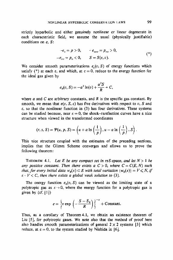
strictly hyperbolic and either genuinely nonlinear or linear degenerate in each characteristic field, we assume the usual (physically justifiable) conditions on e, S:
-e, = P > 0,
-em = PO < 0,
-evuo = puu > 0,
S = S(e, 0). (*)
We consider smooth parameterizations e,(u, S) of energy functions which satisfy (*) at each E, and which, at E = 0, reduce to the energy function for the ideal gas given by
e,(u, S) = -2 In(v) + $ + C,
where a and C are arbitrary constants, and R is the specific gas constant. By smooth, we mean that e(v, S, E) has five derivatives with respect to u, S and E, so that the nonlinear function in (3) has four derivatives. These systems can be studied because, near E = 0, the shock-rarefaction curves have a nice structure when viewed in the transformed coordinates
(r, s, S) = Y(u, p, S) = ( (P)y~-~ln($),S). 24 + a In I
This nice structure coupled with the estimates of the preceding sections, implies that the Glimm Scheme converges and allows us to prove the following theorem:
THEOREM 4.1. Let E be any compact set in r&space, and let N > 1 be any positive constant. Then there exists a C > 0, where C = C(E, N) such that, for every initial data wO(x) c E with total variation { wO(x)} = V < N, if E . V < C, then there exists a global weak solution to (3).
The energy function e,(u, S) can be viewed as the limiting state of a polytropic gas as E -+ 0, where the energy function for a polytropic gas is given by (cf. [ 11)
e= ]uexp (-y) I-‘+Constant.
Thus, as a corollary of Theorem 4.1, we obtain an existence theorem of Liu [5], for polytropic gases. We note also that the method of proof here also handles smooth parameterizations of general 2 x 2 systems [3] which reduce, at E = 0, to the system studied by Nishida in [6].
100 J.BLAKE TEMPLE
1. PRELIMINARIES
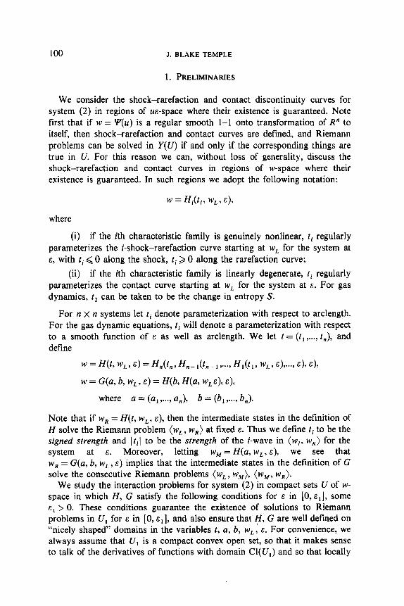
We consider the shock-rarefaction and contact discontinuity curves for system (2) in regions of us-space where their existence is guaranteed. Note first that if w = y(u) is a regular smooth l-l onto transformation of R” to itself, then shock-rarefaction and contact curves are defined, and Riemann problems can be solved in Y(U) if and only if the corresponding things are true in U. For this reason we can, without loss of generality, discuss the shock-rarefaction and contact curves in regions of w-space where their existence is guaranteed. In such regions we adopt the following notation:
where
(i) if the ith characteristic family is genuinely nonlinear, ri regularly parameterizes the i-shock-rarefaction curve starting at wL for the system at E, with ti < 0 along the shock, ti > 0 along the rarefaction curve;
(ii) if the ith characteristic family is linearly degenerate, ti regularly parameterizes the contact curve starting at w, for the system at E. For gas dynamics, t2 can be taken to be the change in entropy S.
For n x n systems let ti denote parameterization with respect to arclength. For the gas dynamic equations, ti will denote a parameterization with respect to a smooth function of E as well as arclength. We let t = (fi,..., f,J, and define
W=H(t,WL,E)=H,(t”,H,_,(t,-1,...,H,(fl, WL,E),...,E),E),
w = G(a, b, w,, E) = H(b, H(u, WOE), E),
where a = (a, ,..., a,), b = (b, )...) b,).
Note that if wR = H(t, wL, E), then the intermediate states in the definition of H solve the Riemann problem (w, , wR) at fixed E. Thus we define ti to be the signed strength and 1 til to be the strength of the i-wave in (w,, w,) for the system at s. Moreover, letting w,,, = H(a, wL, E), we see that wR = G(a, b, w,, E) implies that the intermediate states in the definition of G solve the consecutive Riemann problems (w, , wIM), (We, wR).
We study the interaction problems for system (2) in compact sets U of w- space in which H, G satisfy the following conditions for E in [O,E,], some E, > 0. These conditions guarantee the existence of solutions to Riemann problems in U, for E in [0, sr], and also ensure that H, G are well defined on “nicely shaped” domains in the variables t, a, b, wL, E. For convenience, we always assume that U, is a compact convex open set, so that it makes sense to talk of the derivatives of functions with domain Cl(U,) and so that locally

NONLINEAR HYPERBOLIC CONSERVATION LAWS 101
Lipschitz continuous functions on CI(U,) have uniform Lipschitz bounds. For n x n systems (2), Lemma 1.2 states that such a U, exists in a neighborhood of every u E R”, where E, = 1. For systems (3), we shall show in the next section that every compact set U, in (r, s, S) = w-space satisfies these conditions for some E, > 0.
Conditions (H). There exists a compact convex open set U, I> Cl(U,), and positive constants r < r2 such that, for E in [0, E,], the following hold:
(i) H is defined for every (t, IV,, E) in
r, = {t E R”: Jr,1 <z,} x Cl U, x [0, E,].
00 u2 = Rwe,,,,+ (H) for each fixed w, in Cl U, , E in [0, E,]. U, c RangeItilGT (H) for each fixed w, in Cl U,, E in [0, E,].
(iii) G(I) c U,, where
I-= {a E R”: Ja,J < z} x {b E R”: lbij <z} x Cl U, x [0, E,].
(iv) H, G are C* functions of their arguments, and second derivatives of H, G are locally Lipschitz in I’,, I’, respectively.
(v) H is l-l and IaH/atI # 0 in r, for each fixed w,, E.
Note that Condition (ii) implies that Riemann problems (We, w) are solvable when wL and w are in U,, and E < E, . Condition (v) then implies that we can solve for t in terms of (w, wL, E) in the relation w = H(t, w,, E) when w and wL are in U, , and E < E, . Denoting this function as t = B’(w, wL, E), we can write
where
t = B’(G(a, b, w,, E), w,, E) = B(u, b, w,, E)
= (Bl(a, b, w,, EL.., B,(a, b, w,, ~1,
(u, 2 u,) = (2 = (a, ,***> a,),
(u,, u,) = b = (b, ,..., b,),
(q, UR) = t = c = (c, )...) c,).
For notational convenience, we let c denote the range variable of the function B, which is defined on r. At fixed a, b and w,, we write
C(E) = B(a, b, w,, E),
where C(E) is a function of a, b, w,. Conditions (iv) and (v) imply the following lemma:
LEMMA 1.1. Let U, and E, satisfy the Conditions (H). Then the function

102 J. BLAKE TEMPLE
c = B(a, b, w,, E) is defined, is C2, and second derivatives of B are locally Lipschitz in lY
Proof of Lemma 1.1. By the chain rule, the composition of C2 functions with locally Lipschitz second derivatives, is also a C* function with locally Lipschitz second derivatives. Thus we show that B’ satisfies Lemma 1.1. Consider the equation P(w, t, w, , E) = w - H(t, w, , E) = 0 defined on U, x r,. P is C2 with locally Lipschitz second derivatives in U, x r2. Moreover,
by condition (v), and thus the implicit function theorem implies that t = B’(w, wt, E) is defined locally and has the same smoothness as P. Since P is also l-l at each w, wL, E in U, X U, x [0, ei] by (iv), we have that B’ is globally defined, is C2, and has second derivatives which are locally Lipschitz in U, x U, x [0, E,]. But B(a, b, w,, E) = B’(G(a, b, wL, E), wL, E), and hence B satisfies the conditions of Lemma 1.1. Q.E.D.
We say that two waves a,, bj in a, b approach (cf. Glimm [2]) if i > j, or if i = j and not both a, and bj are positive (i.e., not both ai, bj measure the strengths of rarefaction waves). We define D = D(a, b) to be the sum of the products of the strengths of the approaching waves in a, b, and write this
D = 2: lail 1bjl. APP
(1.0)
For rr x it systems of Eqs. (2), we are interested in estimating the difference between the strengths of the outgoing and incoming waves in the interaction function B; hence we study the functions
ei = ci - a, - b, = Bi(a, b, w,, E) - ai - bi
= Fi(U, b, W, 3 E), (1.01)
where again the domain of Fi is r. It is easy to check (cf. Glimm [ 21) that ei = 0 when D = 0 (since the outgoing waves are then the same as the incoming waves in the corresponding interaction). Moreover
c~(E) - c,(O) = ei(e) - e,(O) = Bi(a, b, W, , E) - Bi(a, b, w,, 0)
is zero when D = 0 or when E = 0. We shall show that this, together with the smoothness properties of B given in Lemma 1.1, imply that
ci=O(a,b,w,,e).D,
where 0 is uniformly bounded, and locally Lipschitz in E uniformly in the

NONLINEAR HYPERBOLIC CONSERVATION LAWS 103
remaining variables. Since the domain of 0 is the compact set r, this will imply that on r,
O(a, b, w, ) E) - O(a, b, w, ) 0) = O( 1)E
and hence the following estimates hold in r for some constant G > 1:
I Ci(e) - Ci(O)l < G&D, ICi-Ui-bil< GD.
(l-1)
One difficulty is the D changes form depending on whether ai and bi are positive an negative. Thus we break the domain r up into regions where D has a fixed form; i.e., regions where sign@,) and sign@,) are constant. Thus we let
and define
s = (SI ,a**> SZJ where si = + or -
r, = {(a, b, wL, E) E R sign@,) = si, sign(b,) = Si+n}.
(For convenience, we allow x = 0 to satisfy sign(x) = si for every si.) Then on r,,
D, = 6, la,41 + Ia,4 + 4 Ia,& + lax&l + Ia,& t 6,lu,b,l t a-. + 6,lu,,b,l
with 6, = (6, ,..., 8,) some sequence of O’s and 1’s. We show that ci = O(u, b, w,, E) D, on each r,, where 0 is bounded and locally Lipschitz in (w,, E) uniformly in a, b. This will imply that the estimates (1.1) hold in each r, and hence on all of r. The proof of the following theorem is the primary goal of the next section: -
THEOREM 1.1. Let w E R” with the setting of system (2). If U, and E, satisfy Conditions (H), then the interaction estimates (1.1) hold for every w, , w,, wR in U,, and E in [0, cl].
The following lemma, whose proof is left to Apendix I, implies that for n x n systems (2), interaction estimates (1.1) holds for every E, in some neighborhood of every u E R”.
LEMMA 1.2. For every u E R”, there exists a neighborhood U, of u such that Conditions (H) hold with E, = 1 and w = u.
Theorem 1.1 and Lemma 1.2 together imply the following theorem, which yields among other things, the main interaction estimates of Glimm [2].

104 .I. BLAKE TEMPLE
THEOREM 1.2. For every u E R”, there is a neighborhood U, of u such that the interaction estimates (1.1) hold for every uL, u,, uR in U, , and every E in [0, 11.
2. INTERACTION ESTIMATES
Let c =f(a, b, z) be defined on the set
W= {a E R”: ai > 0) x {b E R”: bi > 0) X Z with cER’,
where Z c R’ is compact, convex, and is the closure of its interior. Assume that f E C* in Int( IV) with derivatives continuous up to the boundary, and that second derivatives off are locally Lipschitz in W. Further assume that c = 0 when D = 0, where
D=6,a,b,+a2b,+6,a2b2+a,b,+a,b2+6,a,b,+~~~+6,a,b,, (2.1)
where 6 = (6, ,..., S,) is a fixed sequence of O’s and 1’s. The main result of this section is the following theorem:
THEOREM 2.1. If c = f (a, b, z), where f satisfies the conditions above on the domain W, then
c = O(a, 6, z) . D,
where 0 is locally bounded, and locally Lipschitz in z, uniformly in a, b.
We prove this theorem with the aid of the following lemmas. We write
D=(S,a,+a,+.~. +a,)b,+(6,a2+a,+~~~+a,)b2+~~~+6,a,b,.
Letting the coefficients of b, be denoted by d,, we have
6, 1 1 1 -.. 1 0 6, 1 1 *** 1
* 0 0 . a a . . 6,
which we abbreviate as d = Ma, and thus D = Cy=, di bi. This is the setting for the following lemma.
LEMMA 2.1. There exists nonsingular transformations A, B such that a’=Aa,b’=Bb and D = Cy=, a; bj for some m Q n, where A, B are matrices all of whose entries are either O’s or 1’s. Moreover, the image of a

NONLINEAR HYPERBOLIC CONSERVATION LAWS 105
(for a, > 0) under A is the region a’, > ai > --. a; >,O in the first m variables of a’, and for k > m, ai > 0 or 0 < ai < a; for some 1 Q j Q m determines the range of A in the remaining variables. The image of b Gfor bi > 0) under B is the region bi > 0 for 1 < i < m, and for k > m, 0 < b; < b; , for some I,< j < m, determines the range of B in the remaining variables.
Proof: We define A, B by defining each row of A, B. Thus, let Mk, A,, and B, denote the vectors which are respectively the kth rows of M, A, and B. We would like to define A, = Mk, B, = ek = the vector with 1 in the kth spot, zeros everywhere else, so that ai = d,, b: = bi with Ct=i d,b, = D; but whenever ai = 0, ai+ I = 1 we see that di = di+ i, and hence A would not be nonsingular. However, in this case we can write d,b, + di+ 1 bi+ 1 = d,(b, + b,, i). To exploit this idea, we partition the sequence {S, ,..., 6,) into consecutive subsequences of a nice form. Without changing the order of the fS;s, let
16 1,***9 &I = {&,,..., &,I, {&*‘... SJ,..., {Bmp,..., B”J,
s, S2 SP
where, by choosing S, = 0 as needed, we make the following conditions hold on the parity of the indices of {S,}:
For i even:
Si = {0, 0 ,..., 0, 1 } or 0 if i # p.
If 6, = 0, make p even with S, = {0, 0 ,,.., 0).
For i odd: Si = { 1, l,..., 1 } or 0.
It is clear that any sequence of O’s and l’s can be so partitioned. We say loosely that j E S, if mk < j & nk for S, # 0. With this set up, we define A, and B, as follows:
(i) If k = n, or k = nj - 1 for j even with Sj # 0, define
A nj-l =M,,-p A,j = em,,
B nj- 1 = en,-, + e,, B,j = e,.
(ii) Otherwise
A, =Mk,
Bk=ek.
We show that A is nonsingular.

106 J. BLAKE TEMPLE
First, every A, for k E Sj is either Mk or em,. Thus all entries in A, for i < mj are zero, and not all entries from mj to nj are zero. But a quick check shows that every A, such that I& Sj has either ones in the mj - 1 through nj entries, or else zeros in the mj through nj entries (depending on whether A, is a row which is respectively above or below AJ. Thus linear combinations of (A,} have either a constant value in the mj - 1 through nj entries, or else all zeros in the mj through nj entries. Thus A, & Span{A,: I& Sj}. Therefore A is nonsingular if {Amj,..., Anj} are linearly independent for every j such that S, f 0. But this is clearly true forj odd, since then the vectors A,,..., A, are upper triangular with nonzero entries along the diagonal of A. For j even, A,,..., Anj} are linearly independent. Therefore A is a nonsingular matrix all of whose entries are O’s and 1’s.
We show that B is nonsingular.
B, = ek if k # nj - 1 or nj for some j even,
while
Bvj = e,,, Bnj-, = enj+, + %j otherwise.
It is thus clear that {Bk} are linearly independent, and hence B is a nonsingular matrix of O’s and 1’s.
Claim.
D = x ai bi. isdhthat
a;=di
We have that D = Cy= r d, bi. Moreover, for i # nj or nj - 1 for j even, we have
ai = d,,
b; = b,.
But in the other case, d,- , = d,,, which implies that
d,-lb,-, +dn,bn,=d,j-,(bn,-l +b,)=aLj-,bkj-,,
where
aLj- 1 = dnj-, .
NONLINEAR HYPERBOLIC CONSERVATION LAWS 107
Hence
D= i dibi= C dibi + C dnj-l(bnj-l + b,i) i=l i*nj,,nj-I ieven
fOrJC%Jel? Sj+0
= ii a:b; t x a;j-lb;j-, v i*nj,nj-1 jeven
forjeven Aj+ 0
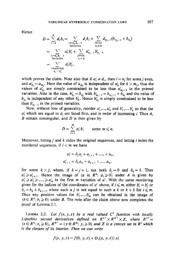
= T‘ a;b;, isuchthat
a;&;
which proves the claim. Note also that if a: # di, then i = nj for somej even, and a:, = ami. Here the value of amj is independent of a; for k > mj, thus the values of aLj are simply constrained to be less than akJ-, in the primed variables. Also in the case, bAj = b, with b’,,- r = b,, r t 6, and the value of b,j is independent of any other b;. Hence b& is simply constrained to be less than bkj-, in the primed variables.
Now, without loss of generality, reorder a; ,,.,, a; and b’, ,..., b; so that the a{ which are equal to di are listed first, and in order of increasing i. Then A, B remain nonsingular, and D is then given by
D = f a; b; some m < n. i=l
Moreover, letting j and k index the original sequences, and letting i index the reordered sequences, if i < m we have
a; = sjuj t uj+ 1 t )...) + a,,
ai+, = 6,a, t ak+, t ,..., a,,
for some k > j, where, if k= j + 1, not both Sj= 0 and 6,= 1. Thus ai > a;,, . Hence the image of {a in R”: a, > 0) under A is given by a’ , , *, ,..., > a:, in the first m variables of a’. With the same reordering > a’ > given for the indices of the coordinates of a’ above, if i < m, either bi = bJ or bi=b,+bk+t, where such a j is not equal to such a k or k t 1 for i < m. Thus any positive values for b;,..., b& can be obtained in the image of {b E R”: bi > 0) under B. The note after the claim above now completes the proof of Lemma 2.1.
LEMMA 2.2. Let f(x, y, z) be a real valued C2 function with locally Lipschitz second derivatives defined on R”+ x R”‘+ x Z, where Rni = (x E R”: xi > 0}, R”+= {y E Rm: yi > 0) and Z is a convex set in R’ which is the closure of its interior. Then we can write
I-(-% YY z) = f(O, Y9 z> + 0,(-T Y, z> II XII

108 J. BLAKE TEMPLE
and
0,(x, Y, z) = 0,(x, 0, z) + 0,(x, Yv z> II YII,
where 0,(x, y, z) is locally bounded and locally Lipschitz in z, uniformly in x and y.
Proof. First, let g(t) be a real valued CN function of the real variable t for t > 0. Then by Taylor’s theorem,
g(t) = g(o) + g’(o)t + ,..., + gcN--l)(0)f + RN,
where
Letting s = ut, ds = t du, we can write
RN = I J & -’ (1 - u)N- ‘fCN’(ut) du 1 p,
- 0
and so for N = 1, we have
g(t) = g(0) + I I1 g'(d) du 1 t. CT,) 0
Now let X be a unit vector in the domain of the variable x. For fixed 2, define
qt, Y, z> =.tw Y, z).
Then by (T,), we can write
qt, y, z) =f(O, Y, z) + O,(t, y, z) * t,
where
O,(t, Y, z) = j’ F&t, y, z> du, 0
where the subscript “(1)” denotes the partial derivative with respect to the first slot variable. Thus, for x = tf we have
f(x, Y, z) =f@, Yv z) + 0,(x, Y9 z) IIXIL

NONLINEAR HYPERBOLIC CONSERVATION LAWS 109
where
01(x, YY z) = j’ & - f(utf, y, z) du
or
0,(x, y, z) = j1 V,,,f(ux, Y, z) . f du, 0
CT,)
where V,,,f denotes the gradient off with respect to the first slot variable. Since 0,(x, y, z) is uniformly bounded by 2 [IVC,,f(O, y, z)ll near x = 0, we can differentiate with respect to y through the integral sign in (T,). Fixing i again, choose a fixed unit vector 7 in the domain of the variable y, and define
0,(x, .% 2) = 0,(x, v, z).
Using Taylor’s theorem again, we obtain
0,(x, s, z) = 0,(x, 0, z) + 0,(x, s, z) - 3,
where, for y = ~7, we have
0,(x, y, z) = j1 Vo,O,(x, uy, z) . Ydu> 0
where V(,,O, denotes the gradient of 0, with respect to the second slot variable. Substituting (T,) into the last equation yields
0*(x, Y9 z) = j' j; V,,,{V,,,.f(ux, uy, z) .2} s jjdu du
or
0,(x, Y, z) = j1 j1 x - [acux;~~uy,, W, UY, 41 . y” du duv Cr,) 0 0 where the expression in brackets denotes the n X m matrix with (i, j)th entry given. Thus, 0,(x, y, z) is uniformly bounded by 2 Il(a’fl8X,@j)(O, 0, z)ll near x = 0, y = 0. That 0,(x, y, z) is locally Lipschitz in z, uniformly in x and y, follows immediately from the hypothesis that
[ a”(x, B.z)J. a4 aYj

110 J.BLAKE TEMPLE
a second derivative off, is locally Lipschitz; i.e., on compact sets,
1 I
< Jj IL zf
0 0 a(uxi> a(uYj) (UT VYY 4 1
- [ a(ux~(~yj) tux, uy, zl)] I/ d” dv <Kllz,-z,II
since
-& (4 Y.Z)] 1 J
is uniformly Lipschitz continuous on compact sets. This completes the proof of Lemma 2.2.
Note that the proof of Lemma 2.2 also goes through if f satisfies the conditions of this lemma on the closure of a domain of the form ~8’ x 9 x Z, where &’ [resp. 91 is a convex subset of R”’ [resp. R”‘], which is the closure of its interior and contains x = 0 [resp. y = 01.
LEMMA 2.3. Let c = f (a, b, a, /?, y, z) be a real valued function which is C2 and has locally Lipschitz second derivatives on a domain Y of the
following form:
a,>a2>.-.>a,>0, 1 <i<n,
bi > 0, I<i<n,
0 < ai < ai or OTi = 0, I<i<n,
O</3,<biorp,=0, I<i<n,
Yi > ak(i) or Yi < Yj for Yj 2 ak(j) or Yi s 03 I<i<m,
z E Z a convex open set in R’.
Then if c = 0 when the inner product a - b = 0 in Y, then
c = O(a, 6, a, p, y, z)a . b
where in Y, O(a, b, y, z) is locally bounded and locally Lipschitz in z,

NONLINEAR HYPERBOLIC CONSERVATION LAWS 111
uniformly in the remaining variables. (The main point here is that Y is convex, and further, if (a, b, a,/?, y, z) is in Y, then the point obtained by letting bi = pi = 0 or a = a = 0 without changing the other entries, is also in
y-1
Proof. We prove this by induction on n. For case n = 1 we have that c = f(a, b, a, /?, y, z) satisfies
f(O, b, 0, P, Y, z) = 0 = f(a, 0, a, 0, Y, z)
in Y a convex set. Since Lemma 2.2 applies to f(a, b, a,/?, y, z) with x = (a, a) and y = (b, p), we can write
f(a, b, a, P, Y, z) = f(O, b, 0,l-h Y, z) + O,(a, b, a, P, Y, z) lb, a)ll,
where
O,(a, b, a,p, y, z) = O,(a, 0, a, 0, Y, z> + O,(a, 6, a,B, Y, z) II(b9P)II
and where O,(a, 6, a,/?, y, z) is locally bounded, and locally Lipschitz in z, uniformly in the remaining variables. Since
0 = O,(a,O, b, 0, Y, z) II@, allI
we have that
f(a, 6, a, P, y, z) = O,(a, b, a, P, Y, z) II@, a>ll WY B)ll.
But since b >/3 and a > a in Y, we have
m= J 0
2
1+ f ’ Il(a,= 2
b a
where each of these is bounded by & in Y. Therefore
f(a, b, a, B, Y, z) = I O,(a, b, a, A Y, 2) Jl+(f)‘JI+(~)‘I a.b
=O,O,a.b=O(a,b,a,jI,y,z)a.b.
Here 0, is bounded by 2 in Y and does not involves the z variables, and so O,O, as well as 0, is locally bounded and locally Lipschitz in z, uniformly in the remaining variables. This proves case n = 1.
We now prove case p = n. Assume Lemma 2.3 is true for p < n - 1, and let
c = f(a, b, a, P, Y, z)
=f(a,,...,a,,b,,..., b,,a,,...,a,,p,,...,Pn,y,z)
505/41/M

112 .I. BLAKE TEMPLE
satisfy the hypotheses of the lemma. Then Lemma 2.2 applies to f with x = (b,, /3,) and y = (a, a), and so we can write
where
f(a, b, a, P, Y, z) = f(a, 0, b, v..., b,, > a, 0, Pz ,..., P,, Y, z)
+ o,@, b, a, A Y, z> II@, 9 PA (A)
O,(~,b,a,~,y,z)=0,(0,b,O,~,y,z)+O2(u,b,a,~,r,z)Il(u,a)l/ (B)
and where 0, is locally bounded and locally Lipschitz in z, uniformly in the remaining variables. But
f@ 1,...,u,,0,b2,...,b,,a,,...,a,,0,~2,...,~,,~,z)
= g(a,,...,a,,b,,...,b,,a,,...,a,,p,,...,p,,a,,a,, r,z>
= g(a’, b’, a’, P’, Y’, z),
where
u’ = (a,,..., a,) is defined on a, > u3 > ,..., > a,,
b’ = (b, ,..., b,) is defined on b, > 0,
a’ = (a,,..., a,) is defined on 0 < oi < Ui or oi E 0,
p’ = v,,...,/?,,) is defined on 0 <pi < bi or pi E 0,
y’=(a,,a,,y)isdefinedfora,<u,foru,>u,.
Since g(u’, b’, a’, p’, y’, z) = 0 when a’ . b’ = 0, g satisfies the hypotheses of this lemma for p = II - 1. So by the induction hypothesis
g(u’, b’, a’, p’, y’, z) = O;(u’, b’, a/,/3’, y’, z) a’ . b’
= O,(u, b, a, P, Y, Z) 2 aibi, cc>
i=Z
where 0; and hence 0, is locally bounded and locally Lipschitz in z, uniformly in the remaining variables on Y. Since a . b = 0 when a = 0, we have from (A) that
O= O,(O, h&P, Y,Z) ll(b,~P,)II
and so combining (A), (B), and (C) yields
f(a, h a, P, Y, Z) = O,(G by a7 A Y, Z> t ui bi i=2
+ o,@, by aTA Y, z) lb, a)li Il(b,~P,N PI
NONLINEARHYPERBOLIC CONSERVATION LAWS 113
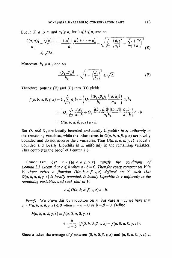
Butin Y,a,>qanda,>qfor l<i<ti,andso
IJ(a,==u~+...+a:+a:+...+a: 01 aI
,<\/2n.
Moreover, b, > /3,, and so
WI VPJI b, =J1+ (gyc\/i (F)
Therefore, putting (E) and (F) into (0) yields
f (a, b, a, 0, y, Z) = 0, i sib, + 02 I
ll@iP,)ll II@, a>ll - i=2 I ail
’ a,bi = OJ-
I i=2 a * b + o, II@, y PA Ilh alI
a,b,
b
= O(a, b, a, @, y, z) a - b.
But 0, and 0, are locally bounded and locally Lipschitz in z, uniformly in the remaining variables, while the other terms in O(a, b, a, /I, y, z) are locally bounded and do not involve the z variables. Thus O(a, b, a, /3, y, z) is locally bounded and locally Lipschitz in z, uniformly in the remaining variables. This completes the proof of Lemma 2.3.
COROLLARY. Let c =f(a, b, a,P, y, z) satisfy the conditions of Lemma 2.3 except that c ,< 0 when a - b = 0. Then for every compact set V in Y, there exists a function O(a, b, a, /I, y, z) d@zed on Y, such that O(a, /I, a, p, y, z) is locally bounded, is locally Lipschitz in z uniformly in the remaining variables, and such that in V,
c 4 O(a, h a, A Y, z) a + b.
proof. We prove this by induction on n. For case n = 1, we have that c=f(a,b,a,/I,r,z),<O when u=a=O or b=p=O. Define
h@, b, a, /A Y, z) = f(a, 0, a9 0, Y, z>
t ~{f(O,b,O,~,y.z)-f(a,O,a,O,y,z)}.
Since h takes the average off between (0, b, 0, P, y, z) and (a, 0, a, 03 Y7 z) at

114 J. BLAKE TEMPLE
fixed (y, z), and since f is negative when a = 0 or b = 0 in Y, we can conclude that
h(a, b, a, /A Y, 2) < 0,
and moreover, h agrees with f when a = a = 0 or b = j3 = 0. Since
! f(O, b, 0, P, y, z) - f(a, 0, a, 0, Y, z)
a+b I
has the smoothness properties off away from a = b = 0, and loses at most one derivative at a = b = 0, it can easily be shown that
--&- {f(O, b, O,P, Y, z) -f(a, 0, a, 0, Y, z)}
and hence h, has the same smoothness as f in Y. Thus,
g(u, b, a, /I?, y, z) = f (a, b, a, P, Y, z> - Nay by a3 03 YY Z>
dominates f, has the smoothness of f, and vanishes when a = a = 0 or b = j? = 0. Therefore, by Lemma 2.3,
g(a, b, a, P, Y, z) = %, b, a, P, y, z) ab
and so
f(a, b, a,P, Y, z> < Wa, b, a,P, Y, z> ah
where o(a, b, a,p, 7, z) is locally bounded and locally Lipschitz in z, uniformly in the remaining variables on Y. This completes the proof of the corollary for case n = 1.
We now prove the case p = n. Assume the corollary is true for p < n and let
c = f (a, b, a, P, Y, z>
= f(a ,,..., a,,, b, ,..., b,,a,,...,a,,p,,...,Pn, Y,Z)
satisfy the hypotheses of the corollary, so that, in particular, c < 0 when the inner product a . b = 0. Let
fi(a, b, a,@, y,z) = f(al ,..., a,,O, b, ,... , b,,al,...,a,,O,p,,...,P,, Y, z),
f&, b, a, p, y, z) = f(a, ,..., a,- ,, 0, bl,..., b,, al,..., a,-Iv &PI v...9P,7 Y, ~1.

NONLINEAR HYPERBOLIC CONSERVATION LAWS 115
But f,(u, b, a, p, y, z) [respectively &,(a, b, a, P, y, z)] is negative when
5 u,bi = 0 respectively “i’ uibi = 0 , i=2 i=l 1
and SO with a renaming of the variables as in the proof of Lemma 2.3, fi satisfies the conditions of the corollary for p = n - 1; i.e.,
fi(~, by a, P, Y, Z) < O,(G 6, a, /A ~3 Z) i aibiy i=2
n-1
f2(a, 6, a, /?, y, Z) < O~(U, b, a, /A 7, Z) C uibi, i=l
where in particular, Oi are locally bounded in Y. These local bounds yield a uniform bound G > 1 on the compact set V, and so we can conclude that
Ata, b, a, P, Y, z) < Ga . b
in V. Now consider the function
(A)
+ ~{h(u,b~a,aY,z)-fi(u,b,a,8.~,z)J
-Gu.b.
As in the case n = 1, h has the same smoothness properties as f, and by (A), h is negative in V. Moreover, h agrees with f in Y when a . b = 0. That is, assuming u - b = 0 in Y, we must have a, b, = 0. If (I, = 0, then since a, > a, > a,, a, = a, = 0, implying that f(a, b, a,/3, y, z) = f2(u, b, a, P, y, z) = h(u, b, a, A Y, z). If b, = 0, then f(u, b, a, P, Y, z) = f,(u, 6, a,@, y, z) = h(u, b, a,/?, y, z).) Therefore we can write
g(a, b, a, P, y, z> = f(a, b, a, P, Y, z) - W b, a, /A Y, z),
where g vanishes in Y when the inner product a . b = 0, and where g has the same smoothness as $ Therefore, by Lemma 2.3,
da, b, a. P, y, z) = O(a, b, a, P, y, z) a - b,
where O(a, b, a, /I, y, z) is defined on Y, is locally bounded, and locally Lipschitz in z uniformly in the remaining variables. Since h is negative in V, we conclude that
f(u, b, a, P, Y, z) Q O@, b, a, P, Y, z) a . b

116 J. BLAKE TEMPLE
in V. This completes the proof of case p = n, and so completes the proof of the corollary.
Proof of Theorem 2.1. We are given the real valued function c = f(a, b, r) which is C* in Int(w) with derivatives continuous up to boundary, and which has locally Lipschitz second order derivatives in W. Further, c = 0 when D = 0, where D is a quadratic term of form given in (2.1). By Lemma 2.1, we can write a’ =Aa and b’ = Bb, where A and B are nonsingular transformations satisfying D = a; b; + e.. + a; bh in W, and such that the image of {a E R”: a, > 0}, {b E R”: bi >, 0) under A, B in the first m variables of a’, b’, respectively, is the set given by
al, 2 a; > * * * > a:, > 0,
b; 2 0, l<k<m.
Moreover, for k > m, we can assume without loss of generality that the image is given by
O<u;<aj forsomel<j<m,
0 Q b; < 6; forsome l<j<m
(this follows since, when a; > 0 defines the image of a; under A for k > m, a case which happens only when 6, = 0 and 6, = 1, the value of a; is independent of the other a; and yet does not appear in the expression for D. In this case ai can be incorporated into the z-variables). Let C denote this image set in the variables a’ and b’.
Let
a” = (a; )...) al,), b” = (b; ,..., b’,),
a = (a, )..., a,) where aj = a; ifu;,ajforj<m,k>m
=o otherwise,
P = (PI v..., P,) where /Ij = b: ifb;<b$forj<m,k>m (2.2)
=o otherwise.
Let Z’ be the domain of (a”, b”, a, /I). Note that .Z’ = C in the nonzero variables of (a”, b”, a, p). Let Y’ = Z’ x 2. Then Y’ satisfies the conditions for the domain Y of Lemma 2.3. Thus we have
c =f(u, b, z) =@-‘a’, B-lb’, z) = g(u”, b”, a, /3, z),
(a”, b”, a, j?, z) E Y’ and c = 0 when u” . b” = 0.

NONLINEAR HYPERBOLIC CONSERVATION LAWS 117
Thus by Lemma 2.3, c = O,(a”, b”, a, p, z) a” - b”, where 0, is locally bounded and locally Lipschitz in z uniformly in a”, b”, a, /3. Thus
c = O,(a”, b”, a, p, z) u” . b” = Ol(u’, b’, z) u” . b” = O&a, Bb, z) . D
= O(a, b, z) . D for (a, b, z) E W.
Since 0, is obtained from 0, by deleting the zero variables among a and p, ,it is clear that 0, is locally bounded and locally Lipschitz in z uniformly in a’, b’. Let Y = C x Z be the image of W under the bijective map CD, where
@:W+ Y,
@(a, b, z) = (AZ, Bb, z).
Let U be a compact convex open subset of W. Then since nonsingular linear transformations preserve compactness and convexity, we have G(U) = V, a compact convex open set in Y. Thus, if (a, b, zI) E U for i = 1,2, and K, A4 are respectively the uniform bound and uniform Lipschitz bound in z for V, we have
lO(a, b, zi)l = IO(A-‘a’, B-lb’, zi)l <it4,
1% b, ~2) - O(a, 6, zl)l = I &(a’, b’, ~2) - O,(a’, b’, ZJ (K I(z2 - z1 11.
Thus O(a, b, z) is locally bounded and locally Lipschitz in z uniformly in Q, b inside W. This proves Theorem 2.1.
COROLLARY 1. Let f (a, b, z) be C2 with locally Lipschitz second derivatives in the domain
V= {a E R”: 0 < a, Q t} x {b E R”:O < b, < t} x Z,
where r is a given positive constant, and Z c R’ is compact, convex and the closure of its interior. Then if c = 0 when D = 0 for some D as given in (2. l), then
c = O(a, b, z) . D,
where 0 is uniformly bounded and uniformly Lipschitz in z on V.
ProoJ The proof of Theorem 2.1 carries through in this restricted domain to imply that c = O(a, b, z) . D, where 0 is locally bounded and locally Lipschitz in z uniformly in a, b. Since V is a compact set, these local bounds imply uniform bounds in V.
COROLLARY 2. Let c = f(a, b, z) be C* with locally Lipschitz second
118 J. BLAKE TEMPLE
derivatives in the domain V above. If c Q 0 when D = 0 for some D as given in (2. l), then there exists a positive constant G > 1 such that
in V.
Proof. Applying the corollary to Lemma 2.3 in the proof of Theorem 2.1 yields the result that c Q O(a, b, z) . D in V, where O(a, b, z) is locally bounded. This proof carries through under the conditions of Corollary 2; i.e., where we only assume that c < 0 when a . b = 0 in V above. The local bounds on O(a, b, z) then imply a uniform bound over the compact set V, which proves that c < GD in V, for some G > 1.
Proof of Theorem 1.1. We have from (1.01)
e, = ci - ai - b, = B,(a, b, wL,e)-ai-b~=Fi(a,b,w,,e).
By Lemma 1.1, B, is C* with locally Lipschitz second order derivatives in r, and hence so is Fi. We apply Corollary 1 of Theorem 2.1 to each I+, c IY Let
fZ= (Iall la,l,..., IanI), 6= (lb,l, lbzl,..., lb,l>,
(2.3)
and let
V={dER”:O<&i<r)X {6’ERn:O<6i<t)XCIU,X [0,&l],
and write
ei = ~~(a, b, w, , E) =f&i, S, w, , ~1 on r, -
Since sign(a,) and sign(b,) are constant on r,,f;: E C* with locally Lipschitz second derivatives in V. Hence, Corollary 1 of Theorem 2.1 applies tofi with z = (wL, E), and so
where 0 is uniformly bounded and uniformly Lipschitz with respect to E in V. Let G, be the maximum of these two uniform bounds and let G = sup,{G,}. Then if (a, b, w,, E) E I’, it is also in some r,, and hence we have
1 eil= If& S, wL, &)I < G,D, Q GD, = GD
NONLINEAR HYPERBOLIC CONSERVATION LAWS 119
and also I Ci(E) - c[(o)l = Ih(& S, wL 9 &) -fr(K S, wL 9 O)l
= 1 O(ci, s, w,, E) - O(& s, w,, O)( D,
Q G,ED, Q GED, = G&D
since D = D, if (a, 6, w,, E) E r,. This proves Theorem 1.1. In the next section, we need estimates on the difference between the
strengths of incoming and outgoing shock and rarefaction waves in the interaction function B. Thus define
z?(q) = 0 if a,< 0
=Q f if a,>0
Y(Ui)=lUil if U,<O
=o if a,>O.
We call R(Ui) the strength of the ith rarefaction wave in Q, and we call y(aJ the strength of the ith shock wave in a. The following two theorems are needed to obtain certain interaction estimates needed in the next section.
THEOREM 2.2. For ci = Bi(a, b, wL, E) defined and C* with locally Lipschitz second derivatives in the compact set r, we have
R (Ci(E)) - R (C,(O)) < G&D,
Y(Ci(e)) - Y(Ci(O>) < G&D,
where G&D is a uniform bound on r.
Proof: We do the case for rarefaction waves. By Theorem 1.1 we have
1 ci(c) - q(O)1 < G&D
on r. Thus Ci(E) - R(ci(O)) ~ cI(E) - C,(O) ~ G&D.
But if ci(s) > 0, then cl(s) = R(Ci(E)) and we have
R(Ci(E)) - R(c,(O)) < G&D,
while if ci(s) < 0, then R(ci(s)) = 0 and we have
R (c~(E)) - R (~~(0)) < 0 < G&D.
This completes the proof of Theorem 2.2.
120 J.BLAKE TEMPLE
THEOREM 2.3. Consider c,. = Bi(a, b, w,, s) defined and C2 with locally Lipschitz second derivatives in the compact set r. Assume that on each I’, we have
R(ci) - R(ai) - R(bi) < 0 when 01 =O,
where 0: is a sum of form (2.1) among a’ = (ai, ,..., a*,) and b’ = (bj, ,..., bj,,,), where {ik}, { jkjs m and 0: depend on s.
Then for some G > 1 we have
R(Ci) - R(ai) - R(bi) < GD’,
Y(Ci) - AaJ - y(bi) < GD’,
where D’ = 0: on r,.
Proof. We do the case for rarefaction waves. Let
ci - R(aJ - R(bJ = B,(a, b, W,, E) -II - R(b,) = hi(a, b, WL, E).
We apply Corollary 2 of Theorem 2.1 to each r, c I’. For each s, we can write
h,(a, b, wi, E) =fi(6’, 6, y, u,, E) =fr(a”, 8, z)
where z = (y, I+, E), y is the vector of all components of a, b not appearing in a’, b’, and q = Ia{ I. Now set
V, = (a” E Rm: 0 < 6; < t} x 16’ E R”‘: 0 <s; <r} x Z.
Since sign(a,) and sign(b,) are constant on rS,fi E C2 with locally Lipschitz second derivatives in VS. Hence, Corollary 2 of Theorem 2.1 applies to J;:, and so
ci - R(a,) - R(bi) Q G,D:,
where G, D, is a bound which holds uniformly in each V,, and so hi(a, b, w,, E) is uniformly bounded by G, . D, on each I’,. Let G = sup,{ G, J. Then if (a, b, w,, E) E r, then (a, b, w,, E) E r, for some s, and so we have
ci - R(a,) - R(bi) < G, 0: < GD’. (2.4)
Now if ci 2 0, then R(ci) = c, and so by (2.4)
R(c,) - R(a,) - R(bi) < GD’,
NONLINEAR HYPERBOLIC CONSERVATION LAWS 121
while if ci < 0, then R(ci) = 0 and so
R(ci) -R(q) - R(bi) < 0 < GD’.
This completes the proof of Theorem 2.3.
3. GAS DYNAMIC EQUATIONS
In this section we study the one-dimensional Lagrangian equations of motion (3) for gas dynamics. This system of equations is determined by specifying the constitutive relation e = e(v, S). We are primarily concerned with energy functions for ideal gases, and for this reason Sections 2-4 of Courant and Friedricks [ 1] are summarized in the following paragraph.
An ideal gas is one that satisfies the equation of state
pv=RT, (3.1)
where p = -e, = pressure, v = specific volume, T = temperature and R = specific gas constant. Moreover, the internal energy gained by the gas during a change of state is equal to the heat contributed to the gas plus the work done on the gas by compressive action of the pressure forces. This fact is expressed by the fundamental relation
de= Tds-pdv. (3.2)
For any given ideal gas, the choice of units for p, v, e, and S together with the molecular weight of the gas determines the constant R. We can take the relation
(3.3)
as the definition of temperature. It is important to note that, since we can only measure changes in energy and entropy, values for e and S at a particular thermodynamic state of the gas are determined only after we choose arbitrary ground states for zero energy and entropy. With these choices, we obtain from (3.2) and (3.3)
de=$dS- pdv, (3.4)

122 J. BLAKE TEMPLE
which yields the linear partial differential equation for e(u, S)
Re, + ve, = 0, (3.5)
the general solution of which is
e = h(v exp(-S/R)), (3.6)
where h is an arbitrary differentiable function. It is also generally true for actual media that
P(V, S) = -e”(V, S) > 0,
P&, S) = -euu(v, S) < 0,
P~V, S) = --euvv(v, 9 > 0.
(3.7)
Hence, for ideal gases, (3.7) is expressed by
h’(x) < 0,
h”(X) > 0, (3.8)
h”‘(X) < 0.
Any gas whose energy function satisfies (3.1~(3.8) we call an ideal gas. A gas is polytropic if further
e=c,T+ C, (3.9)
for some constant c, > 0. The energy function for a polytropic gas is given
e= lvexp (-y) /-‘+CO, (3.10)
where h(x) = exp(-cS,/R)x-’ + C,. For any choice of S, and C, a gas with energy function (3.10) satisfies (3.9) with
For a given polytropic gas, the value of S, is dependent upon our choice of the ground state for entropy, and the arbitrary constant C, in (3.10) is required to adjust for a preassigned choice of ground state for energy.’
For any ideal gas, system (3) can be written
u, + j-(U), = 0, (3.12)
’ The constant C, is usually taken to be zero [ 11, but below we make another choice.

NONLINEAR HYPERBOLIC CONSERVATION LAWS 123
where U = (u, U, E)’ and f(U) = (p, -u, up)‘. (p, -u, up)‘. (p, -u, up)’ is indeed a function of U since (3.6) and (3.8) imply that S = S(e, u) and hence p = p(u, S) = p(u, U, E). The eigenvalues, eigenvectors and Riemann invariants for df are given in (u, U, S) coordinates below. Note that eigen- values and Riemann invariants can be computed in any transformed coor- dinates, but eigenvectors and jump conditions are determined by the variables that yield the conservation form (3.12) of the equations.
R,= (L+=p+~),
R, = (0, e,,, eveus - e,e,,),
R,= 1,~ &--& 3 ( )
1-Riemann invariants S, u - [” fidv,
(3.13)
2-Riemann invariant u, p, (3.13)
3-Riemann invariants S, u + r fidv.
A quick check shows that the equations are genuinely nonlinear in the 1, 3- characteristic fields, and linearly degenerate in the 2-field.
The jump conditions which determine the shock curves for system (3) must be computed from the conservation form of the equations. Letting [u]=u-Mu,, etc., these are
4ul= [PI, u[u] = -[u], (3.14)
m= [PI. Eliminating the shock speed u in the first two equations and requiring the usual entropy conditions (cf. [4]) yields
(3.15)
and eliminating u and u from the third equation yields the Hugoniot relation,
0 = e - eL + +(p + p,)(u - u,). (3.16)
Define the transformation
1 r=U+aln--, s=u-alnl
P P’ (3.17)

124 J. BLAKE TEMPLE
for a > 0 arbitrary. (u, p) + (r, s) defines a one to one and onto regular C” transformation from R x R+ + R x R. Since pv # 0, the transformation
YF (u, p, S) + (r, s, S) (3.18)
determines a one to one and onto regular C” mapping from the domain of the variables (u, u, E) to R3. Hence we can view the shock-rarefaction and contact discontinuity curves of system (3) for any ideal gas, in &-space. Note that since S is a l- and 3-Riemann invariant, and since U, p are 2- Riemann invariants, 1,3-rarefaction curves in &-space lie at constant S, and the 2-contact discontinuity curves are vertical lines parallel to the S axis. We let
w = (r, s, S). (3.20)
For arbitrary constant a and C, consider now the energy function
e,,(u, S) = --a* ln(v exp(-S/R)) + C (3.21)
2
= -a* In ZI + y + C.
e,(u, S) satisfies conditions -(3.1)-(3.5) for an ideal gas with h(x) = -a* In x + C. We now study properties of the shock-rarefaction curves in rsS-space for system (3) with energy function e,(u, S). Since we are soon to consider smooth parameterizations e,(y, s) = e(u, S, a) which reduce to (3.21) at E = 0, we call system (3) with e = e,(u, S) the system at E = 0. We use these special properties together with the estimates of section 2 to prove Theorem 4.1. A corollary of Theorem 4.1 is a Theorem by Liu [ 51 on the existence of solutions to Eqs. (3) for polytropic gases.
Note first that p(u, S) = -e,(u, S) = a’/~ for e,(u, S). Hence Eqs. (3) decouple, and the first two equations here describe the 2 X 2 system studied by Nishida in [6]. Note also that T is a 3-Riemann invariant while s is a l- Riemann invariant for e,(u, S). Thus 1-rarefaction curves lie parallel to the r- axis and 3-rarefaction curves lie parallel to the s-axis. Moreover, the shock conditions (3.15) and (3.16) yield, respectively,
U-uL=-a iup, UUL
S-S,=R
(3.22)
l-shocks are parameterized for 0 < u/u, < 1 while 3-shocks are parameterized for 0 < uL/u < 1. By writing conditions (3.22) in terms of r, s we obtain

NONLINEAR HYPERBOLIC CONSERVATION LAWS 125
l-shock curves:
Cl-l r-rL=a-
\/;; + a In a,
a-l s-sL=a--
6 a In a, O<$=a<l,
S-S,=R I
a*- 1 Ina- ;
I
3-shock curves:
a-l r-rL=a--
6 a In a,
a-l s-sSL=a - + a In a,
\/;; O<:=a<l,
S-S,=--R I
a* - 1 lna-- .
2a I
(3.23)
Thus the shock-rarefaction curves are all the same except that entropy decreases along 3-shocks and increases along l-shocks, as needed to ensure that entropy increases in time. Differentiating (3.23) yields
l-shock curves:
d(s-sL) = ($J;)‘>“, 4r - rL)
O<a=t< 1,
4s - s,> d(r-r,)
=-; (;+ll)*+<o;
3-shock curves:
d(r-rL) = (g+:)*>o, 4s - sd
O<a=:< 1.
4s - s,) 4s - sd
(3.24)
Thus l-shock curves can be parameterized with respect to r - r,, and 3- shock curves with respect to s - s,. Note also that the change in entropy

126 J. BLAKE TEMPLE
along a l-shock [respectively 3-shock] is monotone increasing [respectively decreasing], and on compact sets the change in entropy is uniformly bounded by some constant times r - r, [respectively s - s,].
Since in the rs-plane,the shock curves reduce to those for the isothermal system [6], Riemann problems can be globally solved here by solving them in the rs-plane, and then connecting in the middle by a vertical contact discontinuity. Thus for the energy function e,(u, S), the functions
are everywhere defined as in Section 1, with t, = r - r,, t, = S - S,, t,=s-ss,. Because H, and H, are C’ away from ti = 0, with C2 contact at ti = 0, each Hi is C” with locally Lipschitz second derivatives, and hence so are the functions
w = H(t, wL, 01,
w = G(a, b, wL, O),
where a = (a,, a2, a&, b = (b, , b,, b3) as in Section 2. Moreover
1 I g 20 (3.25)
holds everywhere for e,(v, S), since by (3.24) the shock-rarefaction curves in r&space are nowhere parallel, and vertical vectors are never in the span of two tangent vectors from 1, 3-shock-rarefaction curves. Thus the columns
of aH/at are everywhere independent, so that (3.25) holds. Since H is l-l at fixed w,, (3.25) and the Inverse Function Theorem imply that
t=B’(w, w,,O)
as well as the interaction function
c=t=B(a,b,w,,O) (3.26)
are everywhere defined, and everywhere C* with locally Lipschitz second derivatives. We wish to distinguish i-shocks from i-rarefaction waves among the waves in the interaction function (3.26), so let us adopt the following notation meaningful at any E where B is defined:

NONLINEAR HYPERBOLIC CONSERVATION LAWS 127
aI = the l-shock in a, = 0 if a,>0
=la,l if a, GO, (3.27)
,u, = the I-rarefaction wave in a, = a, if a,>0
=o if a, GO. Similarly let
a, = l-shock in b,, ,+ = I-rarefaction wave in b, ,
p, = 3-shock in u3, f7r = 3-rarefaction wave in u3,
/I2 = 3-shock in b,, q2 = 3rarefaction wave in b,,
164 = 149 I&l = lb& CI’ = l-shock in cr , p’ = 1-rarefaction wave in cr ,
p’ = 3-shock in c,, 77’ = 3-rarefaction wave in c3,
16’) = I cz/ = contact wave in cl.
(3.27)
We let a, P denote arbitrary 1, 3-shocks,
iu, rl arbitrary 1,3-rarefaction waves .
Yi arbitrary shock waves,
Ri arbitrary rarefaction waves,
16il arbitrary contact waves,
4i arbitrary shock or rarefaction waves,
Pi arbitrary waves,
(3.27)
in some solution. The symbols in (3.27) are used to denote both the names as well as the strengths of the corresponding waves (Si denotes signed strength, so that 16,l denotes strength). Let D = the sum of the strengths of the approaching waves among a, b as defined in (l.O), and write
where D=D,+D,+D,,
APP (3.28)
APP
APP

128 J. BLAKE TEMPLE
Finally, letting
w = Hi(tj ,wL 3 O> = (ri(tjT w,! > O), sj(fj, w, 3 O), Sj(tj, w, 3 O)),
define
6, = S,(t, 3 w, 9 0) - s, 2 0,
6, = s, - S&j) WL ,O) > 0.
PROPOSITION 3.1. For every compact set U,, in t-s-space, there exists a constant f < C, < 1 such that every interaction at E = 0 with w,, w,,,, wR in U,, (at any S) satisfies:
6’-a,-6,=0 when D, + D, = 0,
P’-P1-P2<0 when D,=O,
rl’-rll-rtlGo when D, = 0,
a’-a,-a,=A,p’-P,-Pz=B,
where A, B satisfy (I) or (II):
(I) A=-randO<B<C,lorB=-candO<A<C,,&
(II) A < 0 and B Q 0.
The constant C, is determined as follows: Since U,, is compact and shock curves look the same at every entropy level, every Riemann problem in U,, is solvable with shock wave strengths uniformly bounded by a constant P. Set
c = max
I
L d(s-slJ 0 2 ’ d(r - rJ
along a l-shock ; r--lo=p I
i.e., C, is a constant, i Q C, < 1, which dominates the slopes of l-shock curves and reciprocal slopes of 2-shock curves which occur in waves which solve interactions in U,,.
Proof. The results above involving shocks and rarefaction waves are proven via a case by case study of interactions in the rs-plane where strengths are defined. This is given in Appendix II. That 6’ - 6, - 6, = 0 when D, + D, = 0 is a consequence of the fact that when there are no approaching waves among the shocks and rarefaction waves in (wL, w,,,), (Yw wl), the Riemann problems for (wL, wI1) has the same solution waves in the rs-plane. Thus the only change across the interaction is in the contact waves, and hence
NONLINEARHYPERBOLIC CONSERVATION LAWS 129
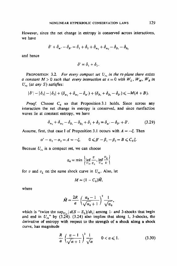
However, since the net change in entropy is conserved across interactions, we have
and hence
PROPOSITION 3.2. For every compact set U,, in the rs-plane there exists a constant M > 0 such that every interaction at e = 0 with W, , W,, W,, in U,, (at any S) satisfies:
Proof: Choose C, so that Proposition 3.1 holds. Since across any interaction the net change in entropy is conserved, and since rarefaction waves lie at constant entropy, we have
6,, + da2 - 6,, -a,, + 6, + 6, = d,, - a,, + 8’. (3.29)
Assume, first, that case I of Proposition 3.1 occurs with A = -<. Then
a’-a,-q=A=-t, O<pl-p,-/3,=B<C&
Because U,, is a compact set, we can choose
a, = min I i~,nfF, inf !L
L fJrs v I
for v and vL on the same shock curve in U,,. Also, let
M = (1 - CO)&,
where
which is “twice the sup”, 1 d(S - S,)/dt,j among l- and 3-shocks that begin and end in U,: by (3.24). (3.24) also implies that along 1, 3-shocks, the derivative of entropy with respect to the strength of a shock along a shock curve, has magnitude
O<a<l. (3.30)

130 .I. BLAKE TEMPLE
Since a decreases along the shock curve as the strength increases, we see that (3.30) and hence the magnitude of this derivative is monotone increasing along shocks. Thus, p’ > 1, f & implies that
60, > &I f s,,. (3.3 1)
that if Moreover, for interactions in U,.,, our choice of M implies a’-a,--*=A=-tthen
is,, + da* - 6, I < $@(.
Hence, using (3.29) together with (3.32) we obtain
(6’ - 6, - 6,) + (S,, + a4* - S,J = 6,, + d,, - 6,s < ;A?(
and so
(8’ - 6, - 6,) t (s,l t s,* - 6,s) + (S,, + is& - a,,)
< $s7( + $I@< = A?(.
Also using (3.29) together with (3.31) we obtain
-(6’ - 6, - 8,) -t (S,, + aa2 - da>) + (d,, - 6,, - 8&) = 0
and
-(sl - 6, - 6,) + (S,, + sa2 - da<) + (6,, + do* - 6,t) < 0.
Putting (3.33) and (3.34) together yields
16’ - 6, - &I+ (S,, + be2 + S,,) + (B& + Jo2 - S,J
< n;ir = M( I - C& < -M(A + 8)
and hence
(3.32)
(3.33)
(3.34)
This proves case (I). For case (II) we have a’ -a,-a,=A<O and /?‘-~,-f?2=B<0.
Thus the estimate (3.32) applies in both cases to yield
NONLINEAR HYPERBOLIC CONSERVATION LAWS 131
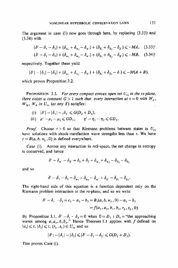
The argument in case (I) now goes through here, by replacing (3.33) and (3.34) with
(6’ - 4 - 4) + (&l + a,, - 6,s) + (S,, + do2 - 6,t) <-MA, (3.33)’
-(s’ - 61 - a,> + &, + a,, - d,t) + (a,, + db2 - d,<) < -MB, (3.34)’
respectively. Together these yield
16’1-1~,l-l6,l+(~,,+6,2-6,,)+(6,,+842-6,)~-M(A+B), which proves Proposition 3.2.
PROPOSITION 3.3. For every compact convex open set U,, in the m-plane, there exists a constant G > 1 such that every interaction at E = 0 with W,, W,, W, in U,, (at any S) satisfies:
(9 l~‘l-l~,l-l~,l~~~~,+~,~~ (ii> P’ -P, -P, < GD,, q’-711-v,<GD,.
Proof. Choose r > 0 so that Riemann problems between states in U,, have solutions with shock-rarefaction wave strengths less than r. We have c = B(a, 6, w,, 0) is defined everywhere.
Case (i). Across any interaction in rsS-space, the net change in entropy is conserved, and hence
and so
6’ - 6, - 6, = 6,* + Be* - 6,< + 6,, - 6,, - f&.
The right-hand side of this equation is a function dependent only on the Riemann problem interaction in the rs-plane, and so we write
6’ - 6, - 6, = c2 -a, - b, = B,(a, b, w,, 0) - a, - b,
=f(a,,a,,b,,b,,r,,s,,O).
By Proposition 3.1, 6’ - 6, - 6, = 0 when 0 = D, + D, = “the approaching waves among a, a,, b, b, .” Hence Theorem 1.1 applies with f defined on Iail < 5, lbil< ~7 (rL, sL) E u,, ad ~0
I~‘l-I~,I-I~,l~I~-~,-~,l~~~~,+~,).
This proves Case (i).
132 J. BLAKE TEMPLE
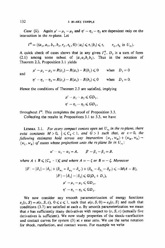
Case (ii). Again ,u’ -,u, -,uuz and ?,I’ - q1 - r12 are dependent only on the interaction in the rs-plane. Let
~=((a~,a~,~~,~~,~~,~~,O):lail~~,I~il~~~ rL,sL in u,,l. A quick check of cases shows that in any given r,“, D, is a sum of form (2.1) among some subset of {a,a,b,b,}. Thus in the notation of Theorem 2.3, Proposition 3.1 yields
and P’ -P, - ru2 = W,) - R(a,) - WI) < 0 when D,=O
v’ - v1 - r2 = WJ -WJ -WA < 0 when D,=O.
Hence the conditions of Theorem 2.3 are satisfied, implying
throughout p. This completes the proof of Proposition 3.3. Collecting the results in Propositions 3.1 to 3.3, we have
LEMMA 3.1. For every compact convex open set U,, in the rs-plane, there exist constants M > 0, i & C, < 1, and G > 1 such that, at E = 0, the following estimates hold across any interaction (wL, ww) + (w,, wR) + (wL, wR) of states whose projections onto the rs-plane lie in U,, :
a’ - a, - a2 = A, P’-P,-/32=&
where A + B Q (C, - l)r and where A = - < or B = - <. Moreover
ld’l- l&l - 1621+ @a, + 6a2 - b> + (S,, + &- d,J < --M(A + B),
16’1-1~,1-1~21~~~~2+~,~~
We now consider any smooth parameterization of energy functions e&v, S) = e(v, S, E), 0 <E < 1, such that e(v, S, 0) = e,(v, S) and such that conditions (3.7) are satisfied at each E. By smooth parameterization we mean that e has sufficiently many derivatives with respect to (v, S, E) (actually five derivatives is sufficient). We now study properties of the shock-rarefaction and contact curves for system (3) at E near zero. We use the same notation for shock, rarefaction, and contact waves. For example we write

NONLINEARHYPERBOLIC CONSERVATION LAWS 133
PROPOSITION 3.4. Let U, be any compact convex open set in rsBspace. Let
r=infr, F=supr, s=infs, F= sups. UI UI Ul UI
Then there exists an E, > 0 such that, for 0 < E < E, , l- and 3-shock- rarefaction curves starting in U,, can be parameterized with respect to r - r,, s - s,, respectively, in a neighborhood of U, as folows:
I-shock-rarefaction curves are defined for ] r - rL. I< F- r, w, E U, by
s--L=fi(r-rL,wWL,E)
S-S,= gl(r-rL,wLtE) (3.35A)
3-shock-rarefaction curves are defined for 1 s - s, 1 < 5- s, wL E U, by
r-rL=f3(s-sSL,wL,E)
s-s,= g,(s-S,,W,,E) (3.35B)
Moreover, (3.35A) and (3.36A) dej?ne the functions
w = (r, s, S) = (r, s, +fi(r - rL, w, , E), S, + g,(r - r, v we v E)) E H;(r - r, , wL, e), (3.36A)
w=(r,s,S)=(rL+f3(s-sSL,wL,e),s,SL+gJ(s-sSL,wL,e))
=H;(s-s,, w~,E), (3.36B)
where H; [resp. Hi] is defined, is C*, and has locally Lipschitz second order derivatives in [-IF--11, IF-I]] x C]U, X [O,eI] [resp. [-IS--_s], ]s-:]I X CIU, x [O~~lll.
Proof The shock conditions (3.15) and (3.16) for system (3) are
u - u, = - \/<P, - P>(V - VL), (3.15)
0 = e -e, + f(p + pL)(v - vL). (3.16)
Since S, and vt are smooth functions of w, = (rL, sL, S,) it follows that (3.16) can be written as
0 = e - e, + f(p +p,)(v - vL) = h(S - S,, a, w,, E), (3.37)
where a = v/v,. At E = 0 we have by (3.22) that ah/a(S - S,) # 0 and h is
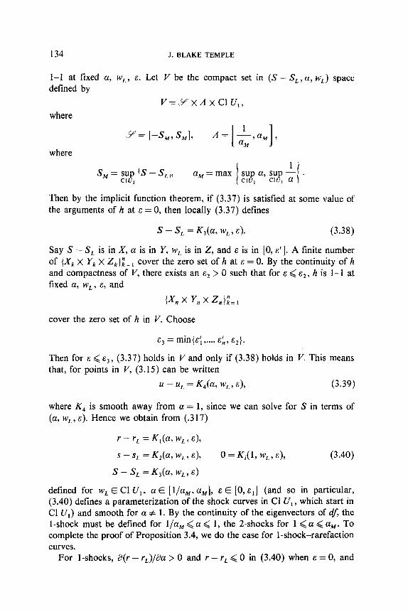
134 J. BLAKE TEMPLE
I-l at fixed a, w,, E. Let V be the compact set in (S - S,, a, wL) space defined by
where
where
Then by the implicit function theorem, if (3.37) is satisfied at some value of the arguments of h at E = 0, then locally (3.37) defines
S - S, = K,(a, wL, E). (3.38)
Say S - S, is in X, a is in Y, wL is in 2, and E is in [0, a’]. A finite number of (X, X Y, X Z,}:!, cover the zero set of h at E = 0. By the continuity of h and compactness of V, there exists an Ed > 0 such that for E < E,, h is 1-I at fixed a, wL, E, and
ix, x yn x Z,l,“= 1
cover the zero set of h in V. Choose
sj = min{e; ,..., EL, al}.
Then for E < Ed, (3.37) holds in V and only if (3.38) holds in V. This means that, for points in V, (3.15) can be written
u - u, = &(a, w,, ~1, (3.39)
where K, is smooth away from a = 1, since we can solve for S in terms of (a, w, , E). Hence we obtain from (.3 17)
r - rL = K,(a, w,, E),
s - sL = &(a, w,, ~1, 0 =K#, wL, E), (3.40)
S-SL=K,(a,w,,c)
defined for wL E Cl U,, a E [l/a M, aM], E E [0, E,] (and so in particular, (3.40) defines a parameterization of the shock curves in Cl U,, which start in Cl U,) and smooth for a # 1. By the continuity of the eigenvectors of df, the l-shock must be defined for l/a, < a < 1, the 2-shocks for 1 < a < aM. To complete the proof of Proposition 3.4, we do the case for I-shock-rarefaction curves.
For l-shocks, a(r - rJLJa > 0 and r - rL < 0 in (3.40) when E = 0, and
NONLINEAR HYPERBOLIC CONSERVATION LAWS 135
hence the inverse function theorem implies that globally, K, defines
a=KS(r-rL, WL,O) in V. (3.41)
Thus the continuity of K, together with the compactness of V implies that in some neighborhood [0,&i] of E=O, a=K, (r-rTL.,wL,a) with r--r,<0 holds if and only of (3.40) holds in V with I - r, < 0. Hence we have
s-sL=f,(r--L,wL,e), S - S, = g, (r - r,, WI., -51,
r<r,, (3.42)
where at each w,E Cl U,, and E in [0, si], (3.42) is defined on some interval r < r < r, which parameterizes the l-shock curve in U, starting from w, at this E. Therefore, without loss of generality, we can assume that (3.42) is defined for r - r, <r - r; wL in Cl U, and E in [0, si]. Note also thatf, and g, are as smooth as e,(v, S, E) and hence are C4 functions.
The 1-rarefaction wave starting at w, for the system at E is the positive portion of the integral curve of the vector field of eigenvectors
R, = (L&u+-+), (3.43)
where R, has at least two less derivatives than e and so is C3. At E = 0 these curves lie along the lines parallel to the positive r-axis, since S and s are I- Riemann invariants at E = 0. Let y(& w,, E) be the 1-rarefaction wave starting at wL for the system at E:
(3.44)
By scaling R, if necessary, we can assume that r parameterizes y with respect to arclength. This defines
r - rL = P,(tl w,, 61,
s - SL = P&, w, ) E),
S-S,=p,(r,w,,E).
(3.45)
Now at E = 0, < = r - r, > 0 and hence (i?r - r-,)/L?< = 1. Let U, be any compact set in rsS-space. Then by the Inverse Function Theorem, there exists an E, > 0 such that for E < E, , c = P,(r - r,, w,, E) throughout U, . Choosing U, large enough, we can write
S--L=fi(r-rL,wL,e),
S-S,= g,(r--L,wL,c), (3.46)

136 .I. BLAKE TEMPLE
where f, and g, are defined for wL in Cl U,, E in [0, ei], and 0 < r - r, < r--r. Hence (3.46) defines a parameterization of the l- rarefaction waves in U, that start in U,, wheref, and g, are again at least c3.
Letting E, be the minimum of this cl and the one found above, we can put (3.42) and (3.46) together to write the 1-shock-rarefaction curves in U, for O<E<E, as
~--~=f,(r-r~,w~,e),
S-S,= gL(r-rL,wL,E), (3.47)
defined for Ir - r,l< F--r, w, in Cl U, and E in [O,E,], where$, and g, are C3 functions for r - r, # 0.
We show that fi and g, are C* at r = r,, and since one sided third derivatives exist at r = rL, this implies that f, and g, are C* with locally Lipschitz second derivatives. Shock curves in U, between 0 and E, are functions of r - r, at a fixed wL in U, , and by Lax [4], the curves defined by (3.47) have C* contact at w,. This implies that first and second derivatives off, and g, with respect to r - r, exist, and are continuous, at r = r,. Since derivatives off, and g, with respect to wL and E are zero from the left and right of r - r, = 0, and Ri(r - r,, wL, E) is differentiable in wL and E, f, and g, are C* at r - r, = 0. Hence f, and g, are C* with locally Lipschitz second derivatives in their domains. This completes the proof of Proposition 3.4.
Let U, and si satisfy Proposition 3.4. We wish to parametrize the 1, 3- shock-rarefaction curves in U, with respect to r - r, + E . arclength [respec- tively s - s, + E . arclength]. Thus let
t,=r-rL+c -H;(r-rL,wL,c) dr,
t3=s-sL+& - H;(r - r,, wL, E) ds.
It is immediate that
at, at3 a(r - rL)
>o and a - SL)
>o
and t, [resp. t3] is a function of (r - r,, w,, E) [resp. (s - sL, w,, E)] which is as smooth as Hi. This implies that ti can be taken to parameterize the i- shock-rarefaction curve; i.e., the Inverse Function Theorem implies that (3.47) defines
r--rL =A,(t,, wL,E), s -SL =A&33 WL, 61,
where Ai are C* with locally Lipschitz second derivatives. Therefore,
NONLINEAR HYPERBOLIC CONSERVATION LAWS 137
substituting into Hi gives the shock-rarefaction curves in U, parametrized with respect to ti at each w, E U,, E E [0, E,]:
(3.48)
where Hi are C2 with locally Lipschitz second derivatives. Moreover, since u and p are 2-Riemann invariants at every E, r and s are constant along 2- contact discontinuity curves. Thus contact discontinuity curves can be smoothly parameterized with respect to t, = S - S,, and we can write
This enables us to define
and
where H, G are C2 with locally Lipschitz second derivatives throughout their domains. Again, the domain and range variables of G determine an interaction with w = We, w, = H(a, w,, E).
Consistent with the notation in (3.27), we let ] tiI be the strength of a wave, and hence in regions where shock-rarefaction curves are parameterized with respect to ti we have
For l-waves a = Var;(a) + E Var(a),
For 3-waves /3 = Vat-;@?) + E Var@),
For 2-waves 6 = AS.
,u = Var,‘@) + E Var@),
q = Var:(q) + s Var(g),(3.49)
(Here, e.g., Var;(a) = the variation of a in the minus r direction.)
PROPOSITION 3.5. For every compact, convex open set U, in r&space, there exists U, 3 U, , 52 > 5 > 0, and E 1 > 0 such that
(i) For each fixed w, in Cl U,, E in [0, el]
Cl U, c Range H(t, w, , E). lfil <r
(ii) For each (a,b,w,,&) in r= {tER3:~t,~<~}2xC1U, x [O,E~],
G(a,hw,,~)~U2.
(iii) For each fixed w, in Cl U, and E in [0, ~~1, H is defined for Itil < f2 and Cl U2 c Range,,il+ H(t, w,, E).

138 J. BLAKE TEMPLE
Proof. Choose U; 2 Cl U,, and r > 0 such that at E = 0,
u; = pa;, m WLY 0) for each fixed wL in Cl U, .
Choose U, such that at E = 0,
Gh b, w,, 0) = u, foreach wLEU;,lail~2t,lbil~22r.
Choose Vi 2 Cl U, and r2 > 0 such that at E = 0
Vi c Range H(t, w,, 0) if/l <(1/2)r2
for each fixed w, in Cl U,.
We claim that there exists an E, > 0 such that (i), (ii), and (iii) hold with the above choices of U,, t, and t2.
First we show that there exists an E, > 0 such that, if E is in [0, E,], then (i) holds. For every w, wL in Cl U,, by choice of r we have w = H(t, wL, 0) for some t with 1 til < r/2. Since
I I g+O at & = 0,
and since by Proposition 3.4 H is defined and continuous in a neighborhood of (t, w,, 0), the Inverse Function Theorem implies that t = B’(w, w,, E) is detined in some neighborhood W x V x [0, E] such that W c U; , Vc U’, and I til < r. Fixing wL , such a W, V, and E exist for every w in Cl U,. A finite number { W, ,..., W,} cover Cl U, since it is compact. Choose P= fi;=, V,, E= min{s , ,..., E,,}. Then for each fixed r? in P and E in [0, E], Cl u, = Rwq,,, Gz H(t, r?, E). Now such a P exists about each w, in Cl U,, so a finite number {P, ,..., FM} cover Cl U, . Choose E, = min{E’, ,..., E’,}. Then for E in [0, si] and fixed w, in Cl U, , we have
Cl U, c Range H(t, wL, E), Ifil<T
which proves (i). Condition (iii) now follows by the same argument. We now show that there exists an E, > 0 such that if E is in [0, ei], then
(ii) holds. Let (a, b, w,, 0) be any point such that I ai] < t, ] bi] < z, and wL is in
Cl U, . Then w = G(u, b, w,, 0) is in U,. Hence, by continuity of G, there exists a neighborhood V of (a, b, wL) and an E > 0 such that
G(Vx [0,c])cU2.
A finite number {Vi,..., V,} cover
(a E R3: Iail <z} x {b E R3: lbil <t} x Cl U,.
NONLINEARHYPERBOLIC CONSERVATIONLAWS 139
Choose E, = min{e , ,..., E,,}. E, clearly satisfied condition (ii). Choosing E, to be the smallest E, from the three cases, Proposition 3.5 follows.
PROPOSITION 3.6. For every compact convex open set U, in &-space, there exists an E, > 0 such that Conditions (H) of Section 1 hold.
Proof: Choose E’,, U,, r, r2 so that Proposition 3.5 holds. At E = 0, IaH/& # 0 and H is globally l-l at each w,, and so by the continuity of H, these conditions also hold in a neighborhood of E = 0 on compact sets. Since r, is compact, Proposition 3.6 follows for some 0 < E, < E;. This proves Proposition 3.6.
Hence, using Lemma 1.1 we can define the interaction function c = B(a, b, w,, E) so that B is C2 with locally Lipschitz second derivatives on r, and such that every interaction that occurs in U, , occurs in this domain of B. For convenience, we now assume that U,, and or, are arbitrary compact convex open sets in rs-space, and that U, and 0, are arbitrary sets of the form U,., x [ $,g] and ur, x [S, $1, respectively. We prove the main interaction lemma for energy functions near e,(v, S).
LEMMA 3.2. For every set U, = U,, x [S, g] in rsS-space there exists E, > 0 and G > 1 such that interactions are defined for every wL, wy and wR in U,, and such that the following estimates hold for these interactions:
(Change in strength at E) < (Change in strength at E = 0) + G&D;
i.e. Aa=a’-a,-a,<AaQ+GeD,
Ap=p’-&-&<A/3°+G~D,
A~6~=~6’~-~61~-~62~~A~6~0+G~D,
Ap=,u’-,u,-pu,<Apo+G~D,
Ay=q’-q,-q,<Ar/“+GeD,
AS, = 6,, + 6,, - 6,, < A6; + G&D,
AS, = 6,, + 6,, - S,, <AS; + G&D.
Proof. We do the proofs for A ] 61, A,u, and AS, ; the others are done similarly. First, let E, be chosen for Proposition 3.6 so that U, , E, satisfy Conditions (H).
Case (i). A 161 <A 16/O + G&D.
Since U,, cl satisfy Conditions (H), Theorem 1.1 applies, and thus across interactions in U, we have
140 J. BLAKE TEMPLE
and thus
1 C*(E) - c,(O)1 = I&(E) - S’(O)1 < G&D
and so 1 d’(e)1 - 1 S’(O)1 < G&D
or IS’@)1 - 141 -lb/ < IS’(O)l- l&l - 14 + G&D
A 161 <A (61°+ G&D.
This proves case (i).
Case (ii). Ap <A,u” + G&D.
Since U,, E, satisfy Condition (H), interactions in U, occur between the states of the interactions function c = I?@, b, w,, E) in the domain r. With the notation of Theorem 2.2, we have
P(E) -P(O) = W,(E)) -W,(O)) G 0
and so Theorem 2.2 applies to yield
which implies
P(E) -P, -P, <P(O) -PU, -~2 + G~J
or
4 Q Ape + GED.
This proves case (ii).
Case (iii). AS, <AS: + G&D. At each E, 6, is the change in entropy along a l-shock curve. Since
w, = (r, s, S) = H,(t, , w, , E) defines the 1-shock-rarefaction curve, we can define s,(t, , wL, E) = S - S, . Of course s&r, w,, E) = 0 when I, = 0 since S = S,. Moreover, 6&r, w,, E) is a C2 function of (tr , w,, E) with locally Lipschitz second derivatives. With this notation we can write
B,,(E) = d,(Cl, w,, E) = J,(B,(a, 6, wt, E), WL, &),
defined on I-. Thus
A~,=~,(~,,~,,~)+~,(~,,w~,~)--~,(c~,w~,~)
= g&, b, w, 3 E)
NONLINEAR HYPERBOLIC CONSERVATION LAWS 141
and
Aa, - AS: = g&, b, w, , E) - g,(a, b, w,, 0)
= f,(a, b, w,, E).
But when D = 0, AS, = 0 and 46: = 0, and hence
f,(a, b, WL, E) = 0.
Also when E = 0, AS: = 0, and again
Since f, is C* with locally Lipschitz second derivatives, Corollary 1 of Theorem 2.1 applies to each I’, to yield
and hence AS, & ASi + G&D. This completes the proof of Lemma 3.2. Without loss of generality, we let G be the same as the one in Lemma 3.1.
LEMMA 3.3. For every set U, = Ur, x [s,S], there exists an M > 0 depending only on Ur,, and an E, > 0 such that, tf wL, w,, E U, , the associated Riemann problem is solvable for each E E [0, E,], and the waves in these Riemann problems satisfy the following estimates:
M Var;(a) > Var(a),
M Var;@) > VartJ),
2 VarJ@) > Var(u),
2 Var:(rt) > Var(r),
Var,cU) < Q,
Var;(a) < a,
Var;GB) < P,
Var; 01) = 0,
Var; (rj) = 0,
V=,(tl) < av.
Proof. These estimates are immediate consequences of the fact that the estimates hold at E = 0, together with the fact that, in some neighborhood of E = 0, Riemann problems in U, are uniquely solvable, and the shock- rarefaction curves that give these solutions depend differentiably on E.
LEMMA 3.4. For every compact set E in rsS-space, there exists a constant 0 < C, < 1 such that, for every B,,(w) with w in E (B,,(w) = ball of radius C,, center w), interaction problems in B,,(w) are solvable for each E E (0, l] with solution waves that satisfy the estimates of Lemma 3.2.
142 J.BLAKE TEMPLE
ProoJ By Theorem 1.1, there is a neighborhood B,(w) about every w in E such that Conditions (H) are satisfied in B,(w). This is all that is needed to obtain Lemma 3.2 for interactions that occurs in B,(w). E being compact implies that a finite number
cover E. Let
n
C,=min + . I I k=l
Then for every w E E, B,,(W) c II,-, for some k, and so Lemma 3.4 follows.
Let E be an arbitrary compact set in rsS-space. Let 0, = or, X [S, $1 be a compact set in r&-space that contains the points within a distance C, of E, C, from Lemma 3.4. Choose tI > 0 so that Lemmas 3.1 to 3.3 apply to 0,. Then Riemann problems ( wL, wR) in 0, are uniquely solvable if E < El,, or if w,, w, E Bcl(w) for w in E and 0 ,< E < 1. Let V, denote the variation in the solution of one of these Riemann problems at any time t > 0.
LEMMA 3.5, With V, defined as above, there exists a constant K, > 1 such that
Proof Since the waves in the solutions of Riemann problems above have uniformly bounded total variation, the lemma is only interesting when (( wL - wRJ( is small. But the existence of a K, in a neighborhood of every (w, E) E 8, x [0, 1 J follows from the strict hyperbolicity of the equations, together with the continuity of the eigenvectors with respect to E. The compactness of 0, x [O, 1) then implies the existence of a uniform constant K,, as desired.
4. EXISTENCE THEOREM USING GLIMM DIFFERENCE SCHEME
We first describe the Glimm difference approximation U,(x, t), h > 0 as described by Liu in [5]. Fix mesh lengths h > 0, 1 > 0 in the x, t directions, respectively. U,, E (r,,, s,, S,) is defined inductively by the following process:
Choose an equidistributed random number ak in (-1, 1) and consider mesh points am,n = ((m + a,) h, nZ), m an integer, m + n even. Now if
NONLINEAR HYPERBOLIC CONSERVATION LAWS 143
U,,(x, t) is defined for 0 < t < nl, we get a piecewise constant function on t = nl, ---co < x < 00, by setting
U,(x, nf) = U,((m + aJh, nl- 0), (m-l)h<x<(m+l)h,
where m + n is even, and then by solving the corresponding Riemann problems we can construct the approximate solution U,(x, t) in the strip nz < t < (n + l)Z, -co < x < co.
In the above process, in order that in each strip nl < t < (n + 1)Z the solutions of the Riemann problems do not interact, we impose the following (Courant-Friedricks-Lewy) condition:
(4.1)
We shall show later such an Z/h > 0 can be chosen for the initial data we consider.
In order to obtain a subsequence of approximate solutions U,, which converges to a solution of system (3), we need to obtain a uniform bound on the total variation of U,,(., t) on each line t = constant > 0. To this end, we need a functional F which measures the total variation of U, along any “Z- curve.” A curve is an Z-curve if it consists of line segments of the form L m,n,mt I,n+ 1) L m,n.m+l.n-l joining a,,,,,, to am+l.n+LT and joining a,,,,,, to a ,,,+ ,,n--l, respectively, and if the mesh index m increases monotonically from -co to +co along such a curve. We can partially order the Z-curves by saying that larger curves lie toward larger time. Let 0 denote the Z-curve passing through the mesh points on t = 0 and t = h. In what follows, J, J, and J, are Z-curves, and J, is the immediate successor of J, if Ji pass through the same mesh points except one with J, < J,. We write J c U, c rsS-space if the states that cross J lie in U,, and we let Var(J) denote the total variation in r, s and S of all the waves that cross J.
Let E be an arbitrarily large compact set in r&-space. We consider now regions U, = U,, x [S, S] that satisfy the conditions in Lemmas 3.1 to 3.4 for some cl > 0, G > 1, M > 1, K, > 1, 0 ( C, < 1. Let
ap(v, s, > “2 O<$(“yf;,, 1 - au
I /( . I 9 ) I
Since U, x [0, 1 ] is compact and ~?p/lav is continuous, such a positive minimum exists. We now consider Z-curves that evolve in U, from initial data in E of total variation V. We wish to choose U, and E, so that, if E . V is sufficiently small, then Z-curves either remain in U, or in B,,(w) some w E E, and Var(J) remains uniformly bounded for all Z-curves J. We obtain
505/41/l IO

144 J.BLAKE TEMPLE
this by showing that a certain functional F which dominates the total variation of the solution on J, decreases. Hence let
L(J)=C~a~-M06~,+Pi-MO~~,}+M~~~6~~+~~{~*+~,}+V, .I J J
L(J)=X iai=M06ai+Pi-Mo84,} tMOJJ6il t EC {/ii+ ?ji} + V, J J .I
Q(J) = M, \' A=
Pil6il t”2 1 4iRi f”3 1 alPi APP APP
J J J
F(J) = LO + &Q(J),
where M,, , M, , M,, and M, are to be chosen later. Since near E = 0, the derivative of the change in entropy with respect to
shock strength goes to infinity along shock curves, we need a bound on the variation of Z-curves in the rs-plane which is independent of M,. To this end we define
LO(J)=x {ai tpi) t vy J (4.3)
Foe(J) = Lo(J) + &Q(J).
LEMMA 4.1. Let U, , E I, and M satisfy the conditions of Lemmas 3.1 to 3.3 as above. Let J, be an Z-curve which evolves at E < E, from initial data wO(x) of variation V, through Z-curves that lie in U,; i.e., assume that for J < J,, J is in U,. Then the following estimates hold for any M,, < 1/2M, and any J, an immediate successor of J, :
6) var,,(J2) < 2OL,(J,);
(ii) VNJ,> < WJ,), where X=$,M,,<& 0
Proof: Since all Z-curves go from w- to w+ (w* = lim,,, m we(x)) we have
so
(Varf (J,) - Var;(J,)I = 1 r+ - r- 1 Q V.
Var: (Jz) Q V + Var;(J,).
Moreover, by Lemma 3.3
(*I
Var,? (J2) > Var,! (1-rarefaction waves) > + 2 ,Ui 3
Var;(Jz) = Var;(2-rarefaction waves) t Var:(shock waves)

NONLINEAR HYPERBOLIC CONSERVATION LAWS 145
where the notation is clear. Hence (*) yields
Similarly
and adding we obtain
(**I
But again by Lemma 3.3 we have
V~r,(JJ G 2 c (a* + Pi) + 2 c Ol, + tl,) J2 Jl
and hence
Var,,(J,) Q 2 c (a, + PJ + 16 (v + c ai + Pi) Jl J2
4 2OJqJ2).
This proves case (i). Next, by Lemma 3.3 we have
Therefore,
Var(J,) < Var(shocks) -I- Var(rarefaction waves) + Var(contact waves)
~MC(aitB,)+2C~i+?i)tClsil
J2 J2 J2
146 J.BLAKE TEMPLE
and by (**)
< 80M*L(J,) =
This completes the proof of Lemma 4.1. Again consider any compact set E in r&space from which our initial
data are chosen. To show that F decreases we need to choose a set U,, containing E, which is independent of the constant K, in Lemma 3.5. We also need ai and pi to dominate Modei and Modoi far away from E = 0. To this end we distinguish between 17, and 8, = or’,, x [& $1, and will choose U, 3 8, depending on estimates we obtain in 8,. Thus let I?,, ti, E;, C, satisfy the conditions of Lemmas 3.1 to 3.5. K, then depends on 0,. Moreover, we have the following lemma.
LEMMA 4.2. Let 8,1 E, cl, A? and C, satisfy the conditions of Lemmas 3.1 to 3.5 as above. Let J, be an I-curve which evolves at E in [0, l] from initial data of variation V, through I-curves that lie in B,,(w) for some w E E; i.e., assume that for J< J,, J is in B,,(w). Then the following estimate holds for any J, an immediate successor of J,, so long as MO sa tisfles : -2
M,<min ?,A =&IO: I I
Var(J,) < WJ,), f&E iv; ’
Proof: Since strengths of waves are defined as in (3.49), we have, for I: > t, )
ai - MO 6,i > Var,(ai) + 6, Var(a,) - G Var(a,)
> $ Var(a,)
NONLINEAR HYPERBOLIC CONSERVATION LAWS 147
and likewise
Therefore,
L(J,) > 2 C { Var(ai) + VW@J} + MO 2 Var(di) J2 J2
+ E”: x {var@i) + var(qi)} > $ Var(J,). J2
If E & E”, , then Lemma 4.1 applies and we have
L(J,) > $ Var(J,).
This proves Lemma 4.2. We now come to the main theorem of Section 4.
THEOREM 4.1. Let E be any compact set in r&space, and let N > 1 be any positive constant. Then there exists a constant C = C(E, N) such that, for every initial data wO(x) c E with TV(w,(x)) = V < N, if EV < C, then there exists a global weak solution to problem (3).
Proof. We show that there exists constants M,, C depending only on E and N, such that, if EV < C, then F bounds the variation of all Z-curves J, F decreases, and Z-curves remain within a region where our estimates hold, and where Condition (4.1) is maintained. In order to be sure that Z14,dai and M,6,, are dominated by the respective shock strengths, we need to do an induction on F0 as well as F. This yields a uniform bound on the variation of all Z-curves that arise from wO(x), and hence by [2,8], implies that there exists a global weak solution to problem (3). First, note that by the definition of wave strength, pi Q 2 Var(pi) for any wave pi, and hence, for any Z-curve J,
x pi 6-x 2 Var(p,) = 2 Var(J), .I J
L(0) < 2 Var(0) + V (‘4)
We now define the constants M,,, M,, M,, M, and C. Let 8, 2 E, t?,, ii?,, K,, and C, be chosen so that Lemmas 3.4, 3.5, and 4.2 hold. Let U,, be the set of points in the rs-plane within a distance of 20(6K,N) of or;,. This

148 J. BLAKE TEMPLE
choice of U,, determines the M and C, of Lemmas 3.1 to 3.3 and Lemma 4.1. Define
M,=min &,a0 , I I
K=max -$,l . I I 0
Let U, = U,, x [S, $1, where
min{dist(0,, S), dist(o,, s)} > 6K,KN.
Choose 0 < E, Q d, and G > 1 so that Lemmas 3.1 to 3.4 and Lemma 4.1 hold with this choice of U,. Let
Let .Z and 0 denote Z-curves that satisfy the conditions of either Lemma 4.1 or 4.2. We have
Var(J) < KL(J) for O<e&l,
V~,,V) < 2oJ5om for E<E,. (B)
Now define
M, = 8G,
M, = 8G + 2M,K(6KoN)G, 63
M, = 8G + 2M,K(6KoN)G + 4M2K(6KoN)G,
and let
K, = 7K;M, N. CD)
Note that Lemma 3.5 implies Var(0) <K, V if E 6 E, or if V < C, . In this case we have by (A)
L(O) < 2 Var(0) + V < 3K, V,
L,(O) Q 2 Var(0) + V< 3K, V.
Moreover, Q(0) < M,(2 Var(0))’ Q 4M, Ki V*, hence
Q(0) < 4M,K;NV< K, V,
and so for O<E< 1,
(E)
(F)
F(0) Q 3K, V + 4M, K;NV < 7K;M, NV = K, V. (G)
NONLINEAR HYPERBOLIC CONSERVATION LAWS 149
Let E,, = min{s, , l/K,}. Then if E < E,, we have E . Q(0) < V and hence
F(0) < 2L(O) < 6K, v,
F,(O) < &(O) < 6K, K &<&,. W
Note here that E,,, M, depend only on E, N. Let C, = e,, C,/K, K. Then if E > s0 and EV < C,, we have KK, V < C,, which by (G) implies
KF(0) < c, for E > sO, (1)
so that C,/K < 1, together with (H), implies that if EV < Cr, then
F(O) < 6&N, for O<e<l.
Finally, let
(J>
C, = min I
(i2M,GK)-’ 1 - C,
K, I ’ 4M,KK, ’
in which case, if EV < C,, then &F(O) < EK, V < K, C, and so
1 -c, &F(O) < (12&f, GK)-’ and &F(O) < 4~~ for 0 < E < 1. (K)
3
Let C = min{C,, C,}. We now prove by induction that with these choices of M,, M, , M2 , M,
and C, if EV < C, then F decreases across successive Z-curves and Z-curves remain within regions where our estimates for Lemmas 3.1 to 3.5, 4.1 and 4.2 hold (i.e., J remains within U, if E < E,,, and within B,,(w) some w E E if s > co). Specifically, we prove by induction that the following inequalities hold at every I-curveJ:
Var(J) < KL(J) < KF(J) < KF(O), for 0 < E < 1,
Var,,(J) < 20&(J) < 2OF,(J) < 2OF,(O) < 20(6K,N), for 0 < E < sO.
Hence, by (I) and (J), all approximate solutions from w,,(x) have uniformly bounded total variation at each E in [0, 11, which by Glimm [2] and Liu [8], implies that there exists a global weak solution to our problem (3). Now if J = 0, then since wO(x) c 0,) and since EV < C, we have from (B) and (H) that for E < E,,,
Var,,(O) < 2OL,(O) < 2OF,,(O) < 20(6K,N),

150 J. BLAKE TEMPLE
implying 0 c U,,. Moreover
Var(0) < KF(0) < 6KK,N,
implying 0 c U,. For E > E,, we have from (B) and (I)
Var(0) <J@(O) < C,
and hence 0 c B,,(w) some w E E. Thus if J = 0, then the desired bounds on Var(J) obtain, and so 0 lies within the regions where our estimates hold. Now let J, be an immediate successor of J,, and let A be the diamond shaped region between J, and J2 in the xt-plane. The states on J2\J, are obtained from the Riemann problem of states (w,, wA) which lie at the lateral vertices of A; and states on J,\J, are obtained from the Riemann problems (wL, w,+,M), (w,,,, wd, where Y,, is the state at the lower vertice of A. Assume by induction that F(J) Q F(0) and F,(J) < I;,(O) for all J < J, (and hence that J c U, for E < e0 or J c B,,(w) for E > E,, o E E). Then across A the interaction ( wL, We) + (w,, We) --t ( wL, wR) occurs, and the estimates of Lemmas 3.1 to 3.3 apply to this interaction. The following estimates are now easily obtained by applying the interaction estimates of Lemma 3.1 to corresponding wave strength differences across A, and including an error of G&D in each case as required by Lemmas 3.2 and 3.4.
<+(A +B)+7GcD<- (1 - Co) 2
< + 7G&D since M, < -&.
MJ2) - ~dJ,) < a’ - aI - a2 +P’ -PI -P2 < (A + B) + 2GeD < -(I - C& + 2GcD.
Q(J,)-Q(J,)<M, C Pi(16’I-I’,j-I’,I)-M*D, Jl\A
+“2 C 4io1’-Pl -P2) JI\p
+M2 C qiol’-Vl-V2)-M2D2 JIV
+ M, C yi(a’ - a, - a2) JI\p

NONLINEAR HirPERBOLIC CONSERVATION LAWS 151
+“3 J% YiV-PI-P2)-“3D3 I
< M, 2 Var(J,){G(D, + D,) + G&D} - 44, D,
+ M,2 Var(J,){GD, + G&D} - M,D,
+ 2M, 2 Var(J,){ G&D} - M,D, + M, 2 Var(J,)r.
By the induction hypothesis, Var(J,) <K&r,) < KF(O), hence
Q<J,> - Q(J,> < 2M,KJ’(O){G(D, + 03) + G&D} --MID, + 4M,KF(O)( GD, + G&D} - M, D,
+ 4M, KF(0) (G&D} - M, D, + M, 2KF(O)<.
The following estimate on F(J,) - F(J,) is obtained by collecting terms with ED, or <, and then factoring them out. Since our estimate for L,(J,) - &,(.I,) is stronger than the one for L(J,) - L(J,), the following estimates will also hold for F&I,) -F&I,).
F(J2)-F(J1)<(7G+4{M1+M2+M3}KG~F(0)-M1}cD1
+ { 7G + 2A4, KF(O)G
+4{M,+M,+M,}KGeF(O)-M,}cD,
+ (7G + 2M,KF(O)G + 4M,KF(O)G
+4(M,+M,+M,JKG&F(O)-M,)&D,
1 - c, 2M,KcF(O) - 2 <.
I
By (K), &F(O) < K, C, which implies that
4(M, + M, + M,} KG&F(O) < 1 and i 2M, K&F(O) -
Moreover, by (J), F(0) < 6K, N and so
F(J2)-F(J,)<{7G+l-M,}ED,
+{7G+2M,K(6KoN)G+1-M,}&D,
+ (7G + 2M,K(6K,N)G + 4M,K(6K,N)G + 1 - M,}ED,
< 0 by our choice of M,, M, and M, in (C).
505/41/1~1 I
152 J.BLAKE TEMPLE
By the note above we also have
F,(J*) - FLdJ,) & 0.
We now can conclude that, if E < cO,
V=,,(J,) Q 2OUJ,) < 2OR,(J,) < 2OR,(J,) < 2OF,(O) Q 20(6K,N)
and hence J2 c U,,. Moreover
Var(J,> < KL(J,) < KF(J,) < KF(J,) < U(O) < 6KK,N
and hence J, c U,. If E,, < E < 1, then
Var(J,) < KL(J,) < KF(J,) < KF(J,) Q KF(0) < C,
and hence J, c B,,(w) some w E E. This concludes the proof of Theorem 4.1.
5, AN EXISTENCE THEOREM FOR POLYTROPIC GASES
In this section we use Theorem 4.1 to prove an existence theorem for polytropic gases, which is essentially the result obtained by Liu in [5]. The main difference here is that Liu does not view the polytropic gas equations as being near the energy function e,(u, S), and moreover, Liu measures the variation of solutions in coordinates that depends on the parameter E which appears in the polytropic gas equations.
The equation for a polytropic gas is given in (3.10). It is important to note that for a given polytropic gas which satisfies (3.9) for some c, = R/E with R and E fixed, the equation for the energy function in (3.10) depends on our choice of ground states for specific entropy S and specific internal energy e. For example, if we fix ground states for S and e, and choose units for v, S, p, and e, then the equation for the energy of our polytropic gas will be
e(u, S) = h(u exp(--S/R)),
where
h(x)= exp -% x-’ + C, ( )
for some (now determined) constant S, and C,. If we were now to change the ground states from which entropy and energy are measured, then the equation for the energy function of this polytropic gas would change, and this change would occur in the constants S, and C,. Moreover, since any

NONLINEAR HYPERBOLIC CONSERVATION LAWS 153
values for the ground states of entropy and energy can be chosen, we can, by an appropriate choice, obtain an equation for the energy function of this gas with preassigned values of S, and C,. Let us choose these ground states so that
and
We now can take
e,(u, S) = ]uexp (-g) I-‘-- 1
E (5-l)
as the energy function of a polytropic gas. But
Fz e,(v, S) = -ln(u exp(-S/R)) = e,(v, S)
and the convergence is smooth in (0, S, E). Thus Lemma 4.1 applies, and we have the following theorem: for any compact set E in M-space and any N > 0, there exists a constant C > 0 such that, if our initial data w,,(x) are in E with total variation { wO(x)} = V Q N, then if SV < C, there exists a global weak solution to problem (3) with energy function (5.1).
APPENDIX I
In this article we prove Lemma 1.2 of section 1, which addresses the local solvability of Riemann problems, as well as the local smoothness of the functions H and B for the general system (2).
LEMMA 1.2. For any ii in the domain of f,(u), there exists a neighborhood U, of ii such that conditions (H) of Section 1 hold with E, = 1.
We prove this with the aid of the following propositions, and refer to the notation of system (2).
PROPOSITION 1. For every ti in the domain of f,(u), there exists a neighborhood U of ii, and a r2 > 0, so that u = H(t, ut, E) is defined, is C2 with locally Lipschitz second derivatives, and satisfies (aHI& ( # 0 in
T, x Ux [0, 11, where T2={tER”:Itil<~,}.
Proof. The eigenvalues of dfE are real and distinct, and letting Ri denote the zth eigenvector of gE, we have that R,(u, E) is a C3 function of its
154 J. BLAKE TEMPLE
arguments. Assume 1 Ri( = 1, and assume that Ri points in the direction of increasing Izi if the ith characteristic field is genuinely nonlinear. Define
U = Hi(ti, UL, E) so that $ = Ri(U, E), I (A)
u = u, if ti = 0,
where ti > 0 if the ith characteristic field is genuinely nonlinear. Then Hi is in C3, and at fixed E, Hi is the arclength parameterization of either the i- rarefaction curve or else the i-contact discontinuity curve starting at u,, for the system at E.
We now show that if the ith characteristic field is genuinely nonlinear, then for any E, there is a neighborhood U x A of (ti, E) such that in U x li, the ith shock curve exists and is defined by
u = Hi(ti9 uL 3 &) for ti < 0,
where Hi is in C3, and at fixed uL and E, Hi is the arclength parameterization of the ith shock curve from uL for the system at E. The jump conditions for system (2) at fixed E are
(u - uL>a = f,(u> -.f&L)~
where u is the shock speed. This can be written as
[G,(u, uL) - u](u - uL) = 0, 03) where
G,(u, u,) = G(u, u,, &I= I l %-A+ + z(u - UL)) dz
0 au
G(u, uL, E) is a C3 function of its arguments, and G(u, uL, E) approaches m>/au LUL as u approaches u,. Moreover, c must be an eigenvalue &(u, uL, E) of G, with u - u, a right eigenvector. Since G(u; ~7, E) = (L?flau)(zi, E), G has real and distinct eigenvalues in a neighborhood W of (ii, ~7, E), and so cr exists in this neighborhood. Note also that r~ = xi(u, u,, E) approaches &(u,, E) as u approaches uL. In W, let &(u, u,,, E) be the left eigenvector for G; i.e., let
&(u, UL 3 6) * G(u> UL 3 &) = Xi(u, UL 3 E) ((UT UL 7 E)
in W.Then,when(B)holdswitha=~i,wehave~~[G-a]~(u-u,)=O, which implies that
(/lj - Ai) 6 * (u - UL) = 0.

NONLINEAR HYPERBOLIC CONSERVATION LAWS 155
Since 5 # xi in W for i #j, (B) holds for u = xi if and only if the following system of n - 1 equations are satisfied:
4 * (u - UL) = 0, i # j. ((3
Since 4 are independent at (17, E, E), the implicit function theorem implies that there exists a neighborhood I/ of (0, ii, E) in which (C) defines a smooth one parameter family of states at each (u,, E), which is as smooth as the 4. By invoking the usual entropy condition of Lax [4] (that A,(u) < xi(u, uL) < Ai on a shock curve), we can now write
U = Hi(ti, UL, E) for -ti < 0, P)
where H is C3 in V and where, at fixed uL and E, (D) defines the arclength parameterization of the i-shock curve from u, for the system at E.
Putting (A) and (D) together, we have the i-shock-rarefaction or contact discontinuity curves defined in a neighborhood of (U; E) by
U=Hi(ti,UL,&) for U,E U, lCi(~72, EEA. 09
Bp,LaxJt], at fixed u, and E, Hi has second derivatives with respect to ti at ti = 0, and by the smoothness of Hi, one-sided third derivatives exist at ci = 0. Since u, = H,(O, U,, E), we also have that at ti = 0, one sided limits of any three derivatives with respect to u, and E exist and are the same. Finally,
uLY E)=Ri(ULY E) and ~(O,u,,E)=~~i.Ri(~LrE) I
have at least three and two derivatives, respectively, with respect to (u,, E), and so H,(t,, uL , E) is a C2 function with locally Lipschitz second derivatives in V. By choosing f2 and U containing Q sufficiently small, we can define
H(t, uL, E) = H,(t,,, H,- ,(t,- , ,..., H&, , u,, E), . . . . E), E)
in T, x U x A, where H is C2 with locally Lipschitz second derivatives. Moreover, since the eigenvectors of u” are linearly independent, ] aH/iYt I# 0 at c = 0, and so we can assume that 1 aH/atI # 0 in T, x U x A and that H is one to one for each fixed u,, E in U x A. Now since [0, l] is compact, a finite number of A’s, say {Ak}trl, cover [0, 11. Therefore, by renaming 7*
and U as
72 = min{zJ~=, and u= fi u,, k=l
we can conclude that H is defined on T, x U x [0, 11, where C is in U and H

156 .I. BLAKE TEMPLE
is C2 with locally Lipschitz second derivatives. This completes the proof of Proposition 1.
PROPOSITION 2. For every 0 ( z < r2, there exists a neighborhood U containing zi, such that, for everyjixed (ZQ, E) in U x [0, 11, we have
U c Rany H(t, uL, E). I T
Proof. Since U = H(0, P, E) and IaH/& 1 # 0 at (0, ~7, E), the inverse function theorem implies that there exists neighborhoods V, W, T, = {t E R,: ] til < r, < r2}, and A, such that
if and only if
u=H(t,uL,e) (F)
t = B’(U, UL) E) (G)
for u in V, u, in W, t in T, and E in A. By the continuity of (G) together with the compactness of A, we can choose U containing C so that
B’(u, uL) E) c {t E R”: 1 tiI ~ 5)
for each fixed uL and E in U x A. Now, again, a finite number of A’s, say lAklL19 cover [0, 11. Therefore, by renaming
u= fi u,, k=l
we have that
U c Rpge H(t, u, , e) i r
for any fixed (uL, E) in U X [0, 11. This completes the proof of Proposition 2.
Proof of Lemma 2.1. By Proposition 2, we can choose U, containing U so that, for each fixed (uL, E) in U, x [0, 11, we have
(I, c Range H(t, u, , E). Itil=GTz
Now choose r < r2 and U’, so that, for (u,, E) in U’ x [0, l] we have
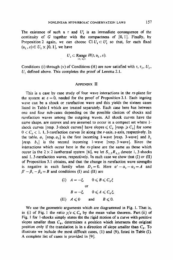
NONLINEAR HYPERBOLIC CONSERVATION LAWS 157
The existence of such a r and U’, is an immediate consequence of the continuity of G together with the compactness of [0, 11. Finally, by Proposition 2 again, we can choose Cl U, c U: so that, for each fixed (u,, E) E U, x [0, 11, we have
Conditions (i) through (v) of Conditions (H) are now satisfied with r, rz , U,, U, defined above. This completes the proof of Lemma 2.1.
APPENDIX II
This is a case by case study of four wave interactions in the rs-plane for the system at E = 0, needed for the proof of Proposition 3.1. Each ingoing wave can be a shock or rarefaction wave and this yields the sixteen cases listed in Table I which are treated separately. Each case here has between one and four sub-cases depending on the possible choices of shocks and rarefaction waves among the outgoing waves. All shock curves have the same shape, are convex and are assumed to occur in a compact set where l- shock curves [resp. 3-shock curves] have slopes < C, [resp. > C,] for some 0 < C, ( 1. 1, 3-rarefaction curves lie along the r-axis,-s-axis, respectively. In the table, a, [resp. a,] is the first incoming l-wave [resp. 3-wave] and b, [resp. b3] is the second incoming l-wave [resp. 3-wave]. Since the interactions which occur here in the r-s-plane are the same as those which occur in the 2 x 2 isothermal system [6], we let S,,,R,*, denote 1,3-shocks and 1,3-rarefaction waves, respectively. In each case we show that (I) or (II) of Proposition 3.1 obtains, and that the change in rarefaction wave strengths is negative in each family when D, = 0. Here a’ - a1 - 01~ =A and p’ -/I, -& = B and conditions (I) and (II) are
(I) A = -6 O<B<C,t or
B=-t;, O<A<C,t,
(II) A<0 and B < 0.
We use the geometric arguments which are diagrammed in Fig. 1. That is, in (i) of Fig. 1 the ratio JJ/Z < C, by the mean value theorem. Part (ii) of Fig. 1 for l-shocks simply states the the rigid motion of a curve with positive slopes smaller than Co, determines a position which intersects the original position only if the translation is in a direction of slope smaller than C,. To illustrate we include the most difftcult cases, (1) and (9), listed in Table (I). A complete list of cases is provided in [9].
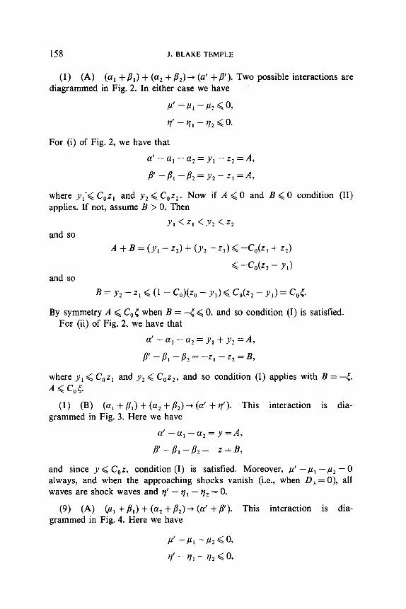
158 .I. BLAKE TEMPLE
(1) (A) (a, + pi) + (a2 + &) + (a’ + p’). Two possible interactions are diagrammed in Fig. 2. In either case we have
P’-Pu,-,&GO,
r’ - ?I - yI2 < 0.
For (i) of Fig. 2, we have that
a’-aI--a,=y,-z,=A,
P-P~-P~=Y~-z,=A,
where yi-< C,z, and y, < C,z, . Now if A < 0 and B & 0 condition (I applies. If not, assume B > 0. Then
Yl < Zl < Y2 < z2
and so
and so
A + B = (Y, - ~2) + (~2 - zd < -W, + 22)
G -C&2 - YJ
B = ~2 - zl< (1 - G,)(z, - Y,) < C&2 - Y,) = GA.
.I)
By symmetry A < C, c when B = -< < 0, and so condition (I) is satisfied. For (ii) of Fig. 2, we have that
a’-a,-a,=y,+y,=A,
pl-/3,-P2=-zl-z2=B,
where y, < C,z, and y, < C0z2, and so condition (I) applies with B = -<, A<C,C
(1) (B) (a, + pl) + (a2 + &) --t (a’ + v’). This interaction is dia- grammed in Fig. 3. Here we have
a’-aa,-a,=y=A,
pl-P,-Pz=-z=B,
and since y < C,,z, condition (I) is satisfied. Moreover, P’ --,LL~ -,u2 = 0 always, and when the approaching shocks vanish (i.e., when D, = 0), all waves are shock waves and q’ - q, - q2 = 0.
(9) (A) (u, + p,) + (a2 +&)+ (a’ + p’). This interaction is dia- grammed in Fig. 4. Here we have
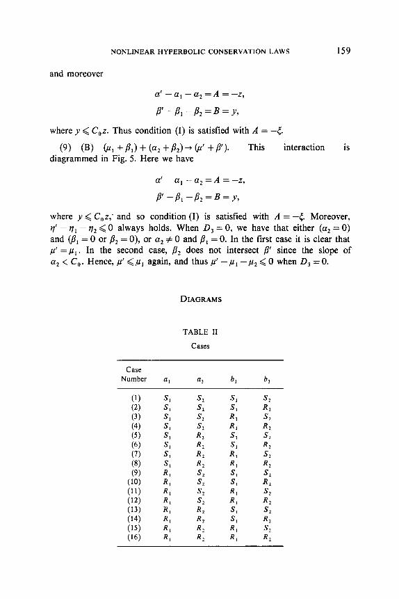
NONLINEAR HYPERBOLIC CONSERVATION LAWS 159
and moreover
a’-a,-a,=A =-z,
P’-PI-Pz=B=y,
where y < C,z. Thus condition (I) is satisfied with A = -r.
(9) 03) Cul +PJ + (a2 +&I -+ 01’ +p’)+ This interaction is diagrammed in Fig. 5. Here we have
a’-a,-aa,=A=-z,
P-B,-&=B=Y,
where y < COz; and so condition (I) is satisfied with A = -<. Moreover, 9’ - q1 - v2 < 0 always holds. When D, = 0, we have that either (a2 = 0) and (/I, = 0 or /I2 = 0), or a2 # 0 and /3, = 0. In the first case it is clear that flu’ =Pl. In the second case, p2 does not intersect p’ since the slope of a2 < C,. Hence, p’ < ,u, again, and thus ,u’ - ,U I --cl2 < 0 when D, = 0.
DIAGRAMS
TABLE II
Cases
Case Number (I, a3 b, b,
(1) s, s* s, s2 (2) s, s* (3) s, s, Rs:
R s:
(4) s, (5) s, Rs:
R s:
R s:
(6) S, R, (7) S, R, ,“;
R S;
(8) (9) R”:
R s:
R s:
R s:
(10) R, S, (11) R, S, ,“:
R S:
(12) R, (13) R, i;
R S;
R S:
(14) R, R, (15) R, R, ,“;
R2
(16) R, R, R, :I
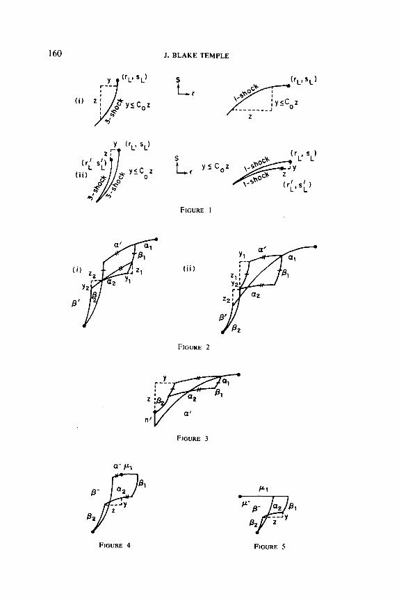
160 J. BLAKE TEMPLE
a’ PP’ Ii)
22 : 21
Y/- r a2 Yl
B
8'
FIGURE 1
(ii)
FIGURE 2
Y r--- Ql
2:
r
Q2 4
a' n’
fi- Q2
63 81
--JY 2
82
FIGURE 4
FIGURE 3
FIGURE 5

NONLINEARHYPERBOLIC CONSERVATION LAWS 161
ACKNOWLEDGMENTS
The author wishes to thank Professor Joel Smaller of the University of Michigan for help and encouragement during the writing of this paper. The author also wishes to acknowledge the papers of Nishida and Smaller [7] and Liu (51 for supplying motivating ideas.
REFERENCES
1. R. COURANT AND K. 0. FRIEDRICKS, “Supersonic Flow and Shock Waves,” Wiley, New York, 1948.
2. J. GLIMM, Solutions in the large for nonlinear hyperbolic systems of equations, Comm. Pure Appl. Math. 18 (1965), 697-715.
3. J. JOHNSON AND J. A. SMOLLER, Global solutions for an extended class of hyperbolic systems of conservation laws, Arch. Rat. Mech. Anal. 32 (1969), 169-189.
4. P. D. LAX, Hyperbolic systems of conservation laws, II, Comm. Pure Appl. Math. 10 (1957), 537-566.
5. TAI-PING Lru, Solutions in the large for the equations of nonisentropic gas dynamics, Indiana Univ. Math. .I. 26, No. 1 (1977).
6. T. NISHIDA, Global solutions for an initial boundary value problem of a quasilinear hyperbolic system, Proc. Japan Acad. 44 (1968), 642-646.
7. T. NISHIDA AND J. A. SMOLLER, Solutions in the large for some nonlinear hyperbolic conservation laws, Comm. Pure Appl. Math. 26 (1973), 183-200.
8. TAI-PING LIU, The deterministic version of the Glimm scheme, Comm. Math. Phys. 57 (1977), 135-148.
9. J. B. TEMPLE, “Solutions in the Large for Some Nonlinear Hyperbolic Conservation Laws of Gas Dynamics,” Ph. D. Dissertation, Univ. of Michigan, 1980.
10. T. NAISHIDA, “Nonlinear Hyperbolic Equations and Related Topics in Fluid Dynamics,” Publications Mathtmatiques D’Orsay, Septembre 1978.
Primed in Belgium