solution to fractional-order riccati di erential equations...

$: Solution to fractional-order Riccati di erential equations ...scientiairanica.sharif.edu/article_21122_82e85ea0d3e882b726867b... · Scientia Iranica D (2019) 26(3), 1608{1616 Sharif$
Scientia Iranica D (2019) 26(3), 1608{1616

Sharif University of TechnologyScientia Iranica

Transactions D: Computer Science & Engineering and Electrical Engineeringhttp://scientiairanica.sharif.edu

Solution to fractional-order Riccati di�erentialequations using Euler wavelet method

A.T. Dincel�

Department of Mathematical Engineering, Davutpasa Campus, Yildiz Technical University, 34220, Esenler, Istanbul, Turkey.

Received 24 June 2018; received in revised form 27 September 2018; accepted 3 October 2018

KEYWORDSEuler wavelet;Fractional calculus;Operational matrix;Numerical solution;Riccati di�erentialequations.

Abstract. The Fractional-order Di�erential Equations (FDEs) have the ability to modelthe real-life phenomena better in a variety of applied mathematics, engineering disciplinesincluding di�usive transport, electrical networks, electromagnetic theory, probability, andso forth. In most cases, there are no analytical solutions; therefore, a variety of numericalmethods have been developed for obtaining solutions to the FDEs. In this paper, we derivenumerical solutions to various fractional-order Riccati-type di�erential equations using theEuler Wavelet Method (EWM). The Euler wavelet operational matrix method converts thefractional di�erential equations to a system of algebraic equations. Illustrative examplesare included to demonstrate validity and e�ciency of the technique.© 2019 Sharif University of Technology. All rights reserved.

1. Introduction

Fractional Di�erential Equations (FDEs) have di�er-entiator operators of non-integer orders. There hasbeen an increasing interest in modeling using FDEs,since they have the ability to model the real-worldphenomena more accurately in a variety of disciplinessuch as visco-elasticity [1], solid mechanics [2], bioengi-neering [3,4], economics [5], continuum mechanics [6],signal processing [7], system analysis [8], optimalcontrol [9,10], and numerical solutions to integraland di�erential equations [11-13]. Since most of thefractional-order di�erential equations do not have ana-lytical solutions, there have been numerous numericalmethods developed to attain solutions to them, includ-ing Adomian Decomposition Method (ADM) [14,15],Variational Iteration Method (VIM) [16], Fourier trans-forms [17], Laplace transforms [18], eigenvector expan-

*. Tel.: +90 212 3834610E-mail address: [email protected]

doi: 10.24200/sci.2018.51246.2084

sion [19], Homotopy Perturbation Transform Method(HPTM) [20,21], and various wavelet methods [22-25].

In many areas of engineering and applied sci-ence, such as transmission-line phenomena, optimal�ltering, network synthesis, robust stabilization, imageprocessing, control theory, etc., Riccati di�erentialequations are utilized. Recently, various numericalmethods [26-29] have been developed to solve Riccatidi�erential equations. As for the numerical methods forfractional Riccati di�erential equations, Yuzbasi [30]developed a numerical method using the Bernsteinpolynomial; Mabood et al. [31] used the OptimalHomotopy Asymptotic Method (OHAM); Li et al. [32]applied a Reproducing Kernel Method (RKM); Odi-bat and Momani [33] used the Modi�ed HomotopyPerturbation Method (MHPM); Khader [34] used thefractional Chebyshev �nite di�erence method; andSakar et al. [35] applied an Iterative ReproducingKernel Hilbert Space Method (IRKHSM) to get thesolutions to fractional Riccati di�erential equations.

In this paper, we consider the following Riccatidi�erential equations of the form:

D�y(t) = u(t) + v(t)y(t) + w(t)[y(t)]2;

A.T. Dincel/Scientia Iranica, Transactions D: Computer Science & ... 26 (2019) 1608{1616 1609

t > 0; n < � � n+ 1; (1)

which is subject to the initial conditions yk(0) = gk andk = 1; 2; � � � ; n�1, where � is the fractional derivative-order parameter; n is an integer; u(t), v(t), and w(t)are given functions; and gk is a constant.

When � is a positive integer, the fractional equa-tion becomes a classical Riccati di�erential equation.

The wavelet theory is one of the popular areasin applied science and engineering, such as segmenta-tion, data compression, and time-frequency analysis.Wavelets generally provide accurate modeling in bothtime and frequency domains. Moreover, it is possible todevelop fast numerical algorithms using wavelets [36].The main advantage of using wavelet methods is that,after the discretization process, the obtained coe�cientmatrix of the algebraic equations is a sparse matrix,which decreases the computational load and expeditesthe simulation.

The focus of this paper is on solving the fractionalRiccati di�erential equations by using Euler wavelets.The Euler wavelets are constructed by Euler polyno-mials. The method consists in reducing the fractionaldi�erential equation to a system of algebraic equationswith unknown coe�cients by using Euler wavelets.Even though the Euler polynomials are not based onorthogonal functions, they have the operational matrixof integration. In addition, numerical examples havedemonstrated that the Euler wavelet performs better inapproximating an arbitrary function than the Legendreand the Chebyshev wavelets do [37].

The structure of the paper is as follows: InSection 2, we present some basic de�nitions andproperties of the fractional calculus. In Section 3,the Euler wavelets are constructed and the EulerWavelets Operational Matrix of the Fractional In-tegration (EWOMFI) is derived. In Section 4, weapply EWM to the solution to the fractional Riccatidi�erential equations through numerical examples; andthe conclusion is presented in Section 5.

2. Preliminary concepts

In this section, we present de�nitions for the prelimi-nary fractional calculus used in the paper.

De�nition 1. The Riemann-Liouville fractional in-tegral operator of order � is given as:

(I�f)(t) =

8><>: 1�(�)

tR0

f(�)(t��)1�� d� � > 0; t > 0;

f(t) � = 0

9>=>; :(2)

For � � 0, � � 0, a � 0, and � � �1, we have thefollowing properties of the Riemann-Liouville fractional

integral:

i) I�I� = I�I�; (3)

ii) I�(I�f(t)) = I�(I�f(t)) = I�+�f(t); (4)

iii) I�(t� a)� =�(� + 1)

�(�+ � + 1)(t� a)�+�: (5)

The Riemann-Liouville fractional derivative is de�nedby:

(D�f)(t) =�ddt

�n(In��f)(t);

0 � n� 1 < � � n; (6)

where n is an integer and t > 0. However, thederivative of the Riemann-Liouville operator has cer-tain shortcomings in modeling real-world phenomena.Therefore, in this paper, we use the modi�ed versionof the fractional di�erential operator D� proposed byCaputo, which is given in the following de�nition.

De�nition 2. The Caputo de�nition of the fractionalderivative operator is given by the following expression:

(D�f)(t)

=

8>>><>>>:dnf(t)dtn � = n 2 R

1�(n��)

tR0

f(n)(�)(t��)1�n+� d� 0�n�1<��n

9>>>=>>>; :(7)

The relation between Riemann-Liouville operator andCaputo operator can be expressed by the following twocommon equations:

(D�I�f)(t) = f(t); (8)

and:

(I�D�f)(t) = f(t)�n�1Xk=0

f (k)(0+)tk

k!: (9)

The reader is referred to [18] for more details aboutfractional di�erentiation and integration.

3. Derivation of the operational matrix offractional integration for Euler wavelets

3.1. Wavelets and Euler waveletsWavelet analysis uses localized wavelike functionscalled `wavelets.' A family of wavelets consists of amother wavelet and dilated and translated versions ofthe mother wavelet. By making the dilation parametera and the translation parameter b vary continuously, we

1610 A.T. Dincel/Scientia Iranica, Transactions D: Computer Science & ... 26 (2019) 1608{1616

can obtain the following family of continuous waveletsas [24]:

a;b(t) = jaj�1=2 �t� ba

�; a; b 2 R; a 6= 0:

(10)

If the translation and dilation parameters are chosento have discrete values, a = a�k0 , b = nb0a�k0 , a0 > 1,b0 > 0, where n and k are positive integers, the familyof discrete wavelets is obtained as:

kn(t) = ja0jk=2 (ak0t� nb0): (11)

Euler wavelets nm = (k; ~n;m; t) have 4 arguments:~n = n�1, n = 1; 2; 3; � � � ; 2k�1; k can take any positiveinteger value; m is the order for Euler polynomials; andt is the normalized time. Euler wavelets de�ned on theinterval [0, 1) yield:

nm(t)

=

(2k�1

2 ~Em(2k�1t�n+1); n�12k�1 � t< n

2k�1

0; otherwise

);(12)

and:

~Em(t) =

8>>><>>>:1; m = 0

1r2(�1)m�1(m!)2

(2m)! E2m+1(0); m > 0

9>>>=>>>; ; (13)

where m = 0; 1; 2; � � � ;M � 1 and n = 1; 2; 3; � � � ; 2k�1.The coe�cient 1r

2(�1)m�1(m!)2(2m)! E2m+1(0)

is for normality,

the dilation parameter is a = 2�(k�1), and the trans-lation parameter is b = ~n2�(k�1). Em(t) representsthe Euler polynomials of the order m and given asfollows [38]:

mXk=0

�mk

�Ek(t) + Em(t) = 2tm; (14)

where�mk

�is the binomial coe�cient. The �rst few

Euler polynomials yield:

E0(t) = 1; E1(t) = t� 12; E2(t) = t2 � t;

E3(t) = t3 � 23t2 +

14; � � � : (15)

3.2. Function approximationA function f(t) de�ned over [0,1) may be expanded by

Euler wavelets as:

f(t) =2k�1Xn=1

M�1Xm=0

cnmnm(t) = CT (t); (16)

where superscript T indicates transposition, and C and (t) are 2k�1 � 1 vectors given as:

C = [c10; c11; � � � ; c1(M�1); c20; c21; � � � ; c2(M�1);

; � � � ; c2k�10; c2k�11; � � � ; c2k�1(M�1)]T ;(17)

= [10;11; � � � ;1(M�1);20;21; � � � ;2(M�1);

; � � � ;2k�10;2k�11; � � � ;2k�1(M�1)]T :(18)

Now, let us de�ne m0 = 2k�1M . The Euler waveletmatrix is de�ned as:�m0�m0 =

�(t1);(t2);(t3); � � � ;(tm0)

�; (19)

where ti represents collocation points. If the colloca-tion points are chosen as ti = i�0:5

m0 , i = 1; 2; 3; � � � ;m0,the Euler wavelet matrix for k = 2, M = 3, and � = 0:5becomes:

�m0�m0(t) =

266666641:4142 1:4142 1:4142�0:2357 0 0:2357�0:0802 �0:1443 �0:0802

0 0 00 0 00 0 0

0 0 00 0 00 0 0

1:4142 1:4142 1:4142�0:2357 0 0:2357�0:0802 �0:1443 �0:0802

37777775 : (20)

3.3. Euler wavelet operational matrix offractional integration

3.3.1. Block pulse functionsAn m0 set of Block Pulse Functions (BPFs) is de�nedas:

bi(t) =

(1 (i� 1)=m0 � t < i=m00 otherwise

); (21)

where i = 1; 2; 3; � � � ;m0. The function bi(t) is disjointand orthogonal. For t 2 [0; 1):

bi(t)bj(t) =

(0 i 6= jbi(t) i = j

); (22)

1Z0

bi(�)bj(�)d� =

(0 i 6= j1=m0 i = j

): (23)

It is known that any square integral function f(t)


de�ned in [0,1) can be expanded into an m0 set of BPFsas:

f(t) =m0Xi=1

fibi(t) = fTBm0(t); (24)

where:

f = [f1; f2; � � � ; fm0 ]T ;Bm0(t) = [b1(t); b2(t); � � � ; bm0(t)]T ;

and fi is given as:

fi =1m0

i=m0Z(i�1)=m0

f(t)bi(t)dt: (25)

The Euler wavelet matrix can also be expanded to anm0 set of BPFs as:

(t) = �m0�m0Bm0(t): (26)

The block pulse operational matrix for fractional inte-gration F� is de�ned as [39]:

(I�Bm0) (t) � F�Bm0(t); (27)

where:

F�=1m�

1�(�+2)

2666666641 �1 �2 �3 � � � �m0�10 1 �1 �2 � � � �m0�20 0 1 �1 � � � �m0�3...

.... . . . . .

......

0 0 � � � 0 1 �10 0 � � � 0 0 1

377777775 ;(28)

with �k = (k + 1)�+1 � 2k�+1 + (k � 1)�+1.Now, let us derive the Euler Wavelet Operational

Matrix of Fractional Integration (EWOMFI):

(I� )(t) � P�m0�m0 (t); (29)

where matrix P�m0�m0 is called the EWOMFI.Using Eqs. (26) and (27), we obtain:

(I�)(t) � (I��m0�m0Bm0)(t)

= �m0�m0(I�Bm0)(t) � �m0�m0F�Bm0(t):(30)

Furthermore, using Eqs. (26), (29), and (30) yields:

P�m0�m0(t) � (I�)(t) � �m0�m0F�Bm0(t)= �m0�m0F��1

m0�m0(t):

The resulting EWOMFI P�m0�m0 becomes:

P�m0�m0 � �m0�m0F��1m0�m0 : (31)

As an example, the EWOMFI for k = 2, M = 3, and� = 0:5 yields:

P�m0�m0 =

266666640:4616 1:2601 �0:97870:0219 0:2243 0:6305�0:0217 �0:1061 0:2354

0 0 00 0 00 0 0

0:5012 �0:6034 0:84250:0179 �0:0449 0:0940�0:0352 0:0410 �0:05450:4616 1:2601 �0:97870:0219 0:2243 0:6305�0:0217 �0:1061 0:2354

37777775 : (32)

We use AB = (aij � bij)m0�m0 for the multiplicationof two matrices of size m0 �m0.

The reader is referred to [37] for the convergenceanalysis of the Euler wavelet basis.

4. Numerical examples

In this section, we provide three numerical examplesto demonstrate the accuracy of the Euler WaveletMethod (EWM). Matlab R2017a has been used forthe simulations. We have also calculated the order ofconvergence, which is expressed as [40,41]:

converg. rate =log�

solution(i�1)�solution(i�2)solution(i�2)�solution(i�3)

�log(2)

: (33)

4.1. Example 1

D�y(t) + y(t)� y2(t) = 0; (34)

with initial condition y(0) = 1=2, where the parameter� denotes the fractional time derivative with 0 < � � 1.The exact solution for � = 1 is given as y(t) = e�t

1+e�t .Let:

D�y(t) � CT (t): (35)

Then, with the initial conditions, we have:

y(t) � (I�D�y)(t) � CTP�m0�m0 (t) + y(0): (36)

Substituting Eq. (26) into Eq. (36) the following isobtained:

y(t) �CTP�m0�m0�m0�m0Bm0(t)

+�

12;

12; � � � ; 1

2

�Bm0(t): (37)

Let:


CTP�m0�m0�m0�m0 = [a1; a2; � � � ; am0 ]; (38)

using Eq. (26), we have:

[y(t)]2 =[a21; a

22; � � � ; a2

m0 ]Bm0(t) + 2KBm0(t)

+�

14;

14; � � � 1

4

�Bm0(t); (39)

where:

K = CTP�m0�m0�m0�m0 �

12;

12; � � � ; 1

2

�: (40)

Substituting Eqs. (39), (37), and (35) into Eq. (34), weget:

CT�m0�m0 + CTP�m0�m0�m0�m0 +�

12;

12; � � � ; 1

2

�� [a2

1; a22; � � � ; a2

m0 ]� 2K ��

14;

14; � � � ; 1

4

�= 0:

(41)

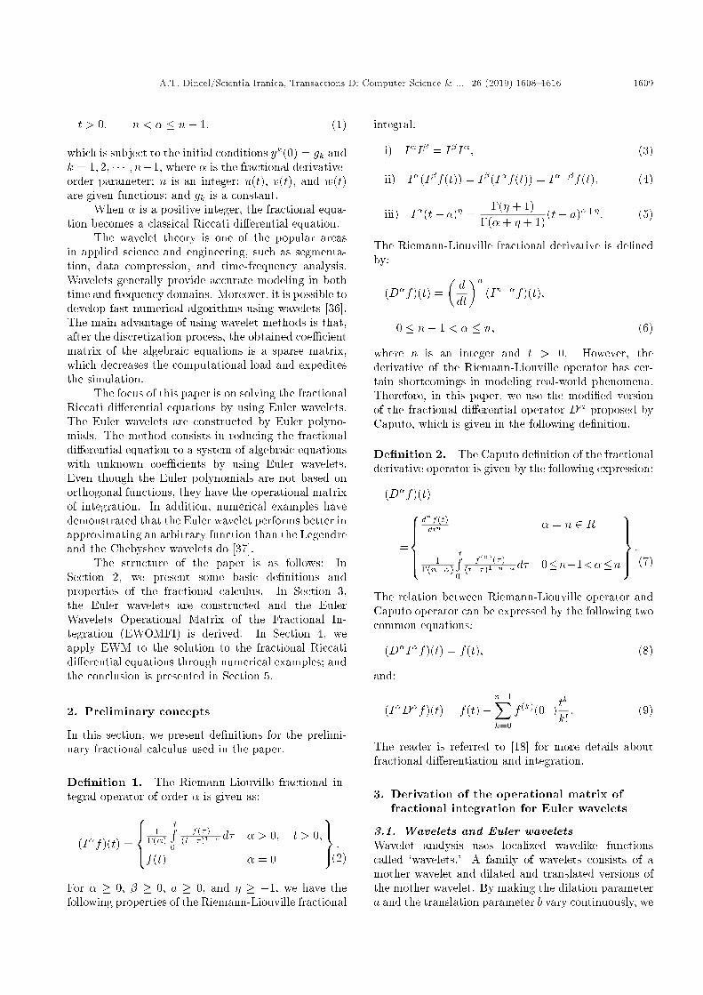
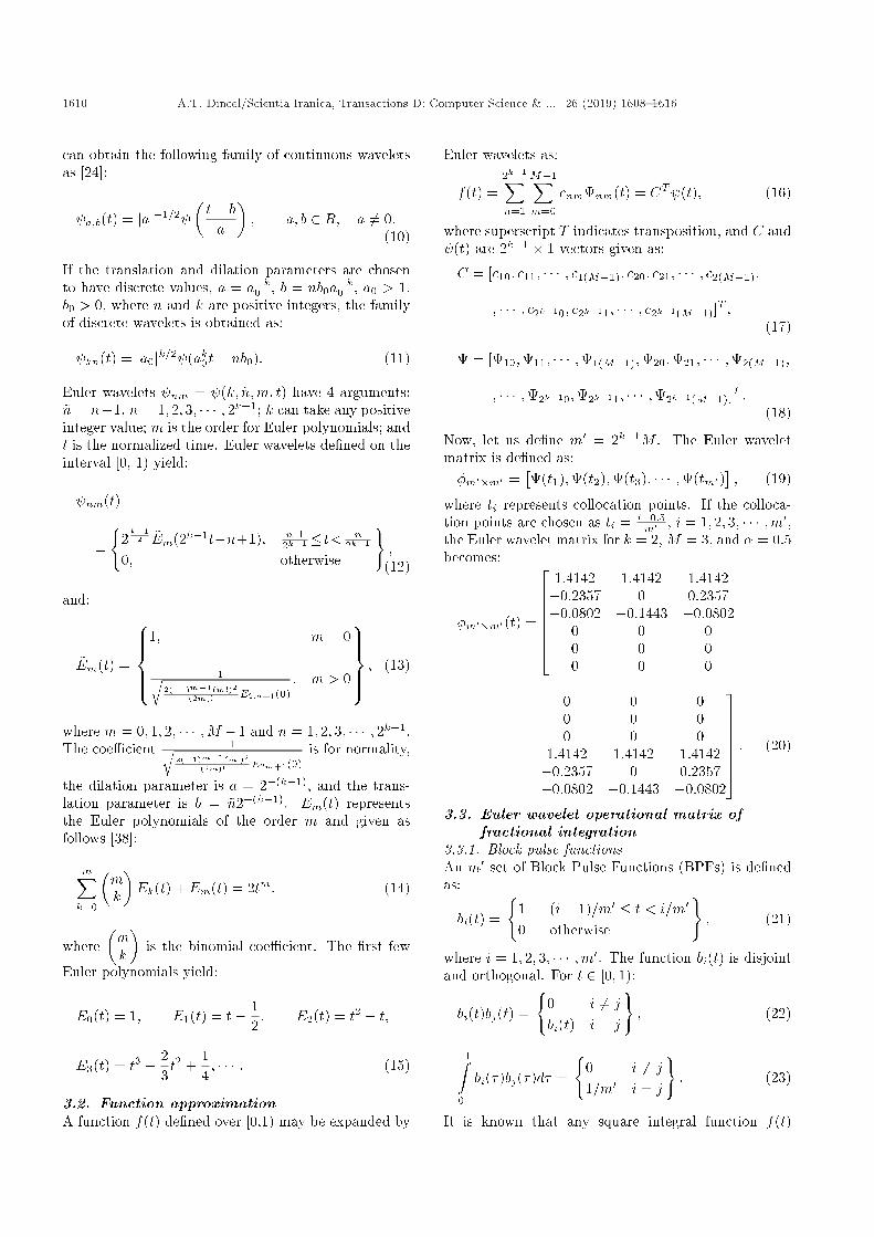
This nonlinear system of equations can be solved usingNewton iteration method and the vector of unknowncoe�cients C can be computed. After calculatingthe vector C, we can obtain the numerical solutionfor y(t) using Eq. (36). Figure 1 shows the EWMsolution for m0 = 80 and the exact solution for � =1. The comparison between the exact solution andEWM solution for various values of m0 is presentedin Table 1. As can be seen in the table, even fairlysmall values of k = 3 and M = 3 (m0 = 12) producea good approximation. As m0 increases, the absoluteerror decreases to the order of E-9. EWM solutionfor m0 = 80 with various fractional values of � isgiven in Figure 2. As � approaches 1, the solutionto the fractional-order di�erential equation approachesthe solution to integer-order di�erential equation. Theorder of convergence is given in Table 2. As it isshown [41,42], this rate tends to 2.

Figure 1. The solution of EWM for � = 1 and the exactsolution for Example 1.

Figure 2. The solution of EWM for various values of �for Example 1.

4.2. Example 2Consider the following Riccati di�erential equation:

D�y(t)� 2y(t) + y2(t)� 1 = 0:

y(0) = 0; (42)

where 0 < � � 1. The exact solution for � = 1 is givenas:

Table 1. Comparison of the exact solution and EWM with � = 1 and various values of m0 for Example 1.

t Exact solution m0 = 12 m0 = 24 m0 = 48 m0 = 96 m0 = 192 m0 = 384

0.0 0.5000000 0.5000223 0.5000028 0.5000004 0.5000000 0.5000000 0.50000000.1 0.4750208 0.4750248 0.4750229 0.4750213 0.4750209 0.4750208 0.47502080.2 0.4501660 0.4501822 0.4501699 0.4501669 0.4501662 0.4501661 0.45016600.3 0.4255575 0.4255764 0.4255623 0.4255588 0.4255578 0.4255576 0.42555750.4 0.4013123 0.4013419 0.4013188 0.4013140 0.4013128 0.4013124 0.40131240.5 0.3775407 0.3775881 0.3775507 0.3775429 0.3775412 0.3775408 0.37754070.6 0.3543437 0.3543778 0.3543529 0.3543460 0.3543443 0.3543438 0.35434370.7 0.3318122 0.3318532 0.3318224 0.3318147 0.3318128 0.3318124 0.33181230.8 0.3100255 0.3100667 0.3100358 0.3100282 0.3100262 0.3100257 0.31002560.9 0.2890505 0.2890953 0.2890613 0.2890532 0.2890512 0.2890507 0.2890505


Table 2. The solution and convergence rate at pointt = 0:5 for Example 1.

i m0 Solution (i) Convergence rate

1 12 0.3775881 |2 24 0.3775507 |3 48 0.3775429 2.26154 96 0.3775412 2.19795 192 0.3775408 2.08746 384 0.3775407 2.0000

y(t) = 1 +p

2 tanh

p2t+

12

log

p2� 1p2 + 1

!!:

Using the same approximation as that given for Ex-ample 1 in detail, we obtain the following nonlinearequation, the solution to which produces C coe�cients:

CT�m0�m0 � 2CTP�m0�m0�m0�m0

+�a2

1; a22; � � � ; a2

m0�� [1; 1; � � � ; 1] = 0: (43)

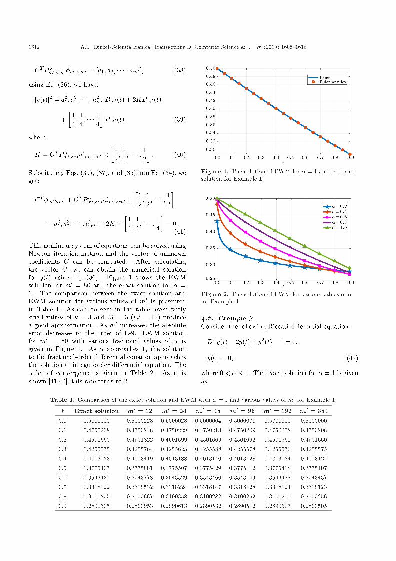
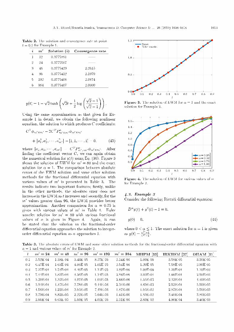
where [a1; a2; � � � ; am0 ] = CTP�m0�m0�m0�m0 . After�nding the coe�cient vector C, we can again obtainthe numerical solution for y(t) using Eq. (36). Figure 3shows the solution of EWM for m0 = 80 and the exactsolution for � = 1. The comparison between absoluteerrors of the EWM solution and some other solutionmethods for the fractional di�erential equation withvarious values of m0 is presented in Table 3. Theresults indicate two important features; �rstly, unlikein the other methods, the absolute error does notincrease in the EWM as t increases and secondly, for them0 values greater than 96, the EWM provides betterapproximation. Another comparison for � = 0:75 isgiven with various values of m0 in Table 4. Eulerwavelet solution for m0 = 80 with various fractionalvalues of � is given in Figure 4. Again, it canbe stated that the solution to the fractional-orderdi�erential equation approaches the solution to integer-order di�erential equation as � approaches 1.



4.3. Example 3Consider the following Riccati di�erential equation:

D�y(t) + y2(t)� 1 = 0;

y(0) = 0; (44)

where 0 < � � 1. The exact solution for � = 1 is givenas y(t) = e2t�1

e2t+1 .

Table 3. The absolute errors of EWM and some other solution methods for the fractional-order di�erential equation with� = 1 and various values of m0 for Example 2.t m0 = 24 m0 = 48 m0 = 96 m0 = 192 m0 = 384 MHPM [33] IRKHSM [27] OHAM [31]

0.1 5.52E-04 1.38E-04 3.43E-05 8.57E-06 2.14E-06 1.00E-06 3.58E-05 3.20E-050.2 6.47E-04 1.63E-04 4.06E-05 1.01E-05 2.54E-06 1.20E-05 7.58E-05 2.90E-050.3 7.27E-04 1.78E-04 4.46E-05 1.12E-05 2.80E-06 1.00E-06 1.20E-04 1.10E-030.4 7.44E-04 1.85E-04 4.56E-05 1.14E-05 2.86E-06 3.03E-04 1.66E-04 2.50E-030.5 5.20E-04 1.52E-04 4.07E-05 1.05E-05 2.66E-06 1.55E-03 2.12E-04 4.40E-030.6 5.84E-04 1.47E-04 3.78E-05 9.44E-06 2.34E-06 4.69E-03 2.52E-04 5.50E-030.7 4.56E-04 1.22E-04 3.05E-05 7.49E-06 1.87E-06 1.05E-02 2.87E-04 5.50E-030.8 3.79E-04 8.82E-05 2.22E-05 5.64E-06 1.41E-06 1.89E-02 3.40E-04 3.80E-030.9 2.66E-04 6.63E-05 1.60E-05 4.02E-06 1.01E-06 2.80E-02 4.90E-04 3.40E-03


Table 4. Comparison of the EWM and some other solution methods for the fractional-order di�erential equation with� = 0:75 for Example 2.

t m0 = 24 m0 = 48 m0 = 96 m0 = 192 m0 = 384 RKM [32] MHPM [33] IRKHSM [35]0.2 0.476341 0.475422 0.475178 0.475117 0.475117 0.4695 0.4288 0.47300.4 0.939340 0.938740 0.938586 0.938548 0.938548 0.9335 0.8914 0.93680.5 1.149579 1.149198 1.149097 1.149070 1.149070 1.1448 1.1327 1.14750.6 1.334765 1.334444 1.334360 1.334339 1.334339 1.3309 1.3702 1.33300.8 1.623300 1.623073 1.623011 1.622995 1.622995 1.6215 1.7948 1.6220

The nonlinear equation used to obtain the coe�-cient vector C becomes:

CT�m0�m0 � [1; 1; � � � ; 1] + [a21; a

22; � � � ; a2

m0 ] = 0;(45)

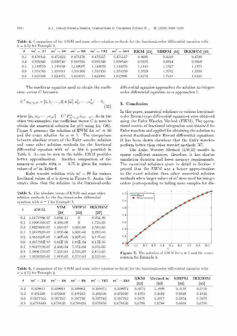
where [a1; a2; � � � ; am0 ] = CTP�m0�m0�m0�m0 . As in theother two examples, the coe�cient vector C is used toobtain the numerical solution for y(t) using Eq. (36).Figure 5 presents the solution of EWM for m0 = 80and the exact solution for � = 1. The comparisonbetween absolute errors of the Euler wavelet solutionand some other solution methods for the fractionaldi�erential equation with m0 = 384 is provided inTable 5. As can be seen in the table, EWM providesbetter approximation. Another comparison of thenumerical results with � = 0:75 is given for variousvalues of m0 in Table 6.

Euler wavelet solution with m0 = 80 for variousfractional values of � is given in Figure 6. Again, theresults show that the solution to the fractional-order

Table 5. The absolute errors of EWM and some othersolution methods for the fractional-order di�erentialequation with � = 1 for Example 3.

t EWM VIM[28]

MHPM[33]

IRKHSM[27]

0.1 1.117589E-07 5.00E-11 0 9.05E-060.2 2.100616E-07 4.39E-09 0 1.72E-050.3 2.822560E-07 1.56E-07 1.00E-06 2.38E-050.4 3.281852E-07 1.97E-06 5.00E-06 2.85E-050.5 3.464860E-07 1.38E-05 3.90E-05 3.11E-050.6 3.307795E-07 6.61E-05 1.93E-04 3.17E-050.7 2.962782E-07 2.43E-04 7.37E-04 3.07E-050.8 2.480617E-07 7.35E-04 2.33E-03 2.81E-050.9 1.922805E-07 1.91E-03 6.37E-03 2.32E-05

di�erential equation approaches the solution to integer-order di�erential equation as � approaches 1.

5. Conclusion

In this paper, numerical solutions to various fractional-order Riccati-type di�erential equations were obtainedusing the Euler Wavelet Method (EWM). The opera-tional matrix of fractional integration was obtained forEuler wavelets and applied for obtaining the solution toseveral fractional-order Riccati di�erential equations.It has been shown elsewhere that the Euler waveletsperform better than other wavelet methods [37].

The Euler Wavelet Method (EWM) results insparse coe�cient matrices; therefore, it has shortersimulation duration and lower memory requirements.The numerical solutions given in detail in Section 4proved that the EWM was a better approximationto the exact solution than other numerical solutionmethods when larger values of m0 were used for integerorders (corresponding to taking more samples for dis-


Table 6. Comparison of the EWM and some other solution methods for the fractional-order di�erential equation with� = 0:75 for Example 3.

t m0 = 24 m0 = 48 m0 = 96 m0 = 192 m0 = 384 RKM[32]

Method in[30]

MHPM[33]

IRKHSM[35]

0.2 0.309815 0.309924 0.309962 0.309972 0.309972 0.3073 0.3099 0.3138 0.31000.4 0.481539 0.481609 0.488162 0.481630 0.481630 0.4803 0.4816 0.4929 0.48160.6 0.5977565 0.597762 0.597780 0.597782 0.597782 0.5975 0.5977 0.5974 0.59780.8 0.6788444 0.678850 0.6788495 0.678850 0.678850 0.6796 0.6788 0.6604 0.6788



cretization). Moreover, the numerical solutions for thefractional orders showed that as � approached 1, theyapproached those for the integer orders. The resultsproved that the method could be applicable to variousother fractional di�erential equations.

The approach used here can be applied to therelated di�erential equations in [43].

References

1. Colinas-Armijo, N., Di Paola, M., and Pinnola, F.P.\Fractional characteristic times and dissipated energyin fractional linear viscoelasticity", Commun. Nonlin-ear Sci. Numer. Simul., 37, pp. 14-30 (2016).

2. Rossikhin, Y.A. and Shitikova M.V. \Application offractional calculus for dynamic problems of solid me-chanics: novel trends and recent results", Appl. Mech.Rev., 63(1), pp. 1-52 (2009).

3. Magin, R.L. and Ovadia M. \Modeling the cardiactissue electrode interface using fractional calculus", J.Vib. Control, 14(9-10), pp. 1431-1442 (2008).

4. Sommacal, L., Melchior, P., Oustaloup, A., Cabelguen,J.M., and Ijspeert, A.J. \Fractional multi-models ofthe frog gastrocnemius muscle", J. Vib. Control, 14(9-10), pp. 1415-1430 (2008).

5. Baillie, R.T. \Long memory processes and fractionalintegration in econometrics", J. Econom., 73(1), pp.5-59 (1996).

6. Carpinteri, A. and Mainardi, F., Fractals and Frac-tional Calculus in Continuum Mechanics, Springer-Verlag, Vien, New York (1997).

7. Lima, M.F.M., Machado, J.A.T., and Cris�ostomo,M. \Experimental signal analysis of robot impacts ina fractional calculus perspective", J. Adv. Comput.Intell. Intell. Inform., 11, pp. 1079-1085 (2007).

8. Chen, C. and Hsiao, C. \Haar wavelet method forsolving lumped and distributed-parameter systems",IEE P-Contr. Theor. Appl., 144(1), pp. 87-94 (1997).

9. Karimi, H., Moshiri, B., Lohmann, B., and Maralani,P. \Haar wavelet-based approach for optimal control of

second-order linear systems in time domain", J. Dyn.Control Syst., 11(2), pp. 237-252 (2005).

10. Sadek, I., Abualrub, T., and Abukhaled, M. \Acomputational method for solving optimal control ofa system of parallel beams using Legendre wavelets",Math. Comput. Model, 45(9-10), pp. 1253-1264 (2007).

11. Babolian, E., Masouri, Z., and Hatamzadeh-Varmazyar, S. \Numerical solution of nonlinearVolterra-Fredholm integro-di�erential equations viadirect method using triangular functions", Comput.Math. Appl., 58(2), pp. 239-247 (2009).

12. Kajani, M. and Vencheh, A. \The Chebyshev waveletsoperational matrix of integration and product opera-tion matrix", Int J. Comput. Math., 86(7), pp. 1118-1125 (2008).

13. Razzaghi, M. and Youse�, S. \The Legendre waveletsoperational matrix of integration", Int. J. Syst. Sci.,32(4), pp. 495-502 (2001).

14. El-Wakil, S.A., Elhanbaly, A., and Abdou, M.A.\Adomian decomposition method for solving fractionalnonlinear di�erential equations", Appl. Math. Com-put., 182(1), pp. 313-324 (2006).

15. Momani, S. and Odibat, Z. \Numerical approach todi�erential equations of fractional order", J. Comput.Appl. Math., 207(1), pp. 96-110 (2007).

16. Das, S. \Analytical solution of a fractional di�usionequation by variational iteration method", Comput.Math. Appl., 57(3), pp. 483-487 (2009).

17. Gaul, L., Klein, P., and Kemple, S. \Damping descrip-tion involving fractional operators", Mech. Syst. SignalPr., 5(2), pp. 81-88 (1991).

18. Podlubny, I., Fractional Di�erential Equations: AnIntroduction to Fractional Derivatives, Fractional Dif-ferential Equations, to Methods of Their Solution andSome of their Applications, New York, Academic Press(1999).

19. Suarez, L. and Shokooh, A. \An eigenvector expansionmethod for the solution of motion containing frac-tional derivatives", J. Appl. Mech., 64(3), pp. 629-635(1997).

20. Kumar, S. \A new fractional analytical approach fortreatment of a system of physical models using Laplacetransform", Sci. Iran. B, 21(5), pp.1693-1699 (2014).

21. Khader, M.M. \Application of homotopy perturbationmethod for solving nonlinear fractional heat-like equa-tions using Sumudu transform", Sci. Iran. B, 24(2),pp. 648-655 (2017).

22. Xu, X. and Xu, D. \Legendre wavelets method forapproximate solution of fractional-order di�erentialequations under multi-point boundary conditions",Int. J. Comput. Math., 95(5), pp. 998-1014 (2018).

23. Wang, Y.X. and Fan, Q.B. \The second kind Cheby-shev wavelet method for solving fractional di�erentialequation", Appl. Math. Comput., 218(17), pp. 8592-8601 (2012).


24. Shah, F.A. and Abass, R. \Haar wavelet operationalmatrix method for the numerical solution of fractionalorder di�erential equations", Nonlinear Engin., 4(4),pp. 203-213 (2015).

25. Rahimkhani, P., Ordokhani, Y., and Babolian, E.\Numerical solution of fractional pantograph di�er-ential equations by using generalized fractional-orderBernoulli wavelet", J. Comput. Appl. Math., 309(1),pp. 493-510 (2017).

26. El-Tawil, M.A., Bahnasawi, A.A., and Abdel-Naby,A. \Solving Riccati di�erential equation using Ado-mian's decomposition method", Appl. Math. Comput.,157(2), pp. 503-514 (2004).

27. Sakar M. \Iterative reproducing kernel Hilbertspacesmethod for Riccati di�erential equations", J. Comput.Appl. Math., 309, pp. 163-174 (2017).

28. Batiha, B., Noorani, M.S.M., and Hashim, I. \Applica-tion of variational iteration method to general Riccatiequation", Int. Math. Forum, 2(56), pp. 2759-2770(2007).

29. Geng, F., Lin, Y., and Cui, M. \A piecewise varia-tional iteration method for Riccati di�erential equa-tions", Comput. Math. Appl., 58(11-12), pp. 2518-2522(2009).

30. Yuzbas�, S. \Numerical solutions of fractional Riccatitype di�erential equations by means of the Bernsteinpolynomials", Appl. Math. Comput., 219(11), pp.6328-6343 (2013).

31. Mabood, F., Ismail, A.I., and Hashim, I. \Appli-cation of optimal homotopy asymptotic method forthe approximate solution of Riccati equation", SainsMalays., 42(6), pp. 863-867 (2013b).

32. Li, X.Y., Wu, B.Y., and Wang, R.T. \Reproducingkernel method for fractional Riccati di�erential equa-tions", Abstr. Appl. Anal., Article ID 970967, 6 pages(2014).

33. Odibat, Z. and Momani, S. \Modi�ed homotopy per-turbation method: application to quadratic Riccatidi�erential equation of fractional order", Chaos Soli-tons Fractals, 36(1), pp. 167-174 (2008).

34. Khader, M.M. \Numerical treatment for solving frac-tional Riccati di�erential equation", J. Egyptian Math.Soc., 21(1), pp. 32-37 (2013).

35. Sakar, M.G., Akg�ul, A., and Baleanu, D. \On solu-tions of fractional Riccati di�erential equations", Adv.Di�er. Equ., 39, pp. 1-10 (2017).

36. Beylkin, G., Coifman, R., and Rokhlin, V. \Fastwavelet transforms and numerical algorithms", I.Commun. Pure Appl. Math., 44(2), pp. 141-183(1991).

37. Wang, Y. and Zhu, L. \Solving nonlinear Volterraintegro-di�erential equations of fractional order byusing Euler wavelet method", Adv. Di�er. Equ., 27,pp. 1-16 (2017).

38. He, Y. and Wang, C. \Recurrence formulae forApostol-Bernoulli and Apostol-Euler polynomials",Adv. Di�er. Equ., 209, pp. 1-16 (2012).

39. Kilicman, A. \Kronecker operational matrices for frac-tional calculus and some applications", Appl. Math.Comput., 187(1), pp. 250-265 (2007).

40. Atkinson, K.E., An Introduction to Numerical Analy-sis, Wiley, New York (1978).

41. Majak, J., Shvartsman, B., Karjust, K., Mikola, M.,Haavaj oe, A., and Pohlak, M. \On the accuracy of theHaar wavelet discretization method", Compos. Part B,80, pp. 321-327 (2015).

42. Majak, J., Pohlak, M., Karjust, K., Eerme, M.,Kurnitski, J., and Shvartsman, B.S. \New higherorder Haar wavelet method: Application to FGMstructures", Compos. Struct., 201, pp. 71-78 (2018).

43. Tural Polat S.N. \The vector-matrix form numericalsimulations for time-derivative cellular neural net-works", Int. J. Numer. Model., 31(5), pp. 1-13 (2018).

Biography

Arzu Turan Dincel received the PhD degree inMathematical Engineering from the Yildiz TechnicalUniversity, Istanbul, Turkey. She is currently anAssistant Professor in the Mathematical EngineeringDepartment of Yildiz Technical University. Some of herresearch interests include fractional calculus, fracturemechanics, and �nite element method.

solution to fractional-order riccati di erential equations...

Documents