solution methods for quadratic...
TRANSCRIPT

Solution Methods forQuadratic Optimization
Robert M. Freund
April 4, 2002

Outline�Pivoting Algorithms for Quadratic Optimization
� Interior-Point Methods for Quadratic Optimization
�Active Set Methods for Quadratic Optimization
�Reduced Gradient Algorithm for QuadraticOptimization
�Some Computational Results
c�2002 Massachusetts Institute of Technology. All rights reserved. 15.094 1

Pivoting Algorithms forQuadratic Optimization
Quadratic Problem
Consider the following format for QP:��� ����������
����� ���
��� �� � � ��
� � � ��
Associate multipliers � and � with the constraintsabove.
c�2002 Massachusetts Institute of Technology. All rights reserved. 15.094 2

Pivoting Algorithms forQuadratic Optimization
KKT Conditions
��� ��������
������ ���
�� � �� � � ���
� � � ��
The KKT optimality conditions for QP are:
� �� ��� � � �
� � �
��� ����� � � � �
� � �
� � �
���� � � � � � � � �
���� � � � � � � � ��
c�2002 Massachusetts Institute of Technology. All rights reserved. 15.094 3

Pivoting Algorithms forQuadratic Optimization
The Tableau
� �� ��� � � �
� � �
��� ��� � � � �
� �
� � �
��� � � � � �� ��
���� � � � � �� � �
Write the first five conditions in the form of a tableau of linearconstraints in the nonnegative variables �� � ���:
� � � � Relation RHS
� � �� �� � �
� � �� � � ��
� � � � � � � � � � � �
c�2002 Massachusetts Institute of Technology. All rights reserved. 15.094 4
Pivoting Algorithms forQuadratic Optimization
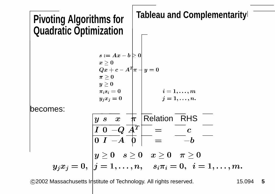
Tableau and Complementarity
� �� ��� � � �
� � �
��� ��� � � � �
� �
� � �
��� � � � � �� ��
���� � � � � �� � �
becomes:
� � � � Relation RHS
� � �� �� � �
� � �� � � ��
� � � � � � � � � � � �
���� � � � � � � � � ���� � � � � � � � ��
c�2002 Massachusetts Institute of Technology. All rights reserved. 15.094 5

Pivoting Algorithms forQuadratic Optimization
Basic Feasible Solutions
� � Relation RHS
� � �� �� � �
� � �� � � ��
� � � � � � � � � �
��� � �� � �� � � � � �� ��� � �� � � �� � � � ���
This tableau has exactly ����� rows and ������ columns.
Any basic feasible solution (BFS) will have exactly one half of thecolumns in the basis.
We can find a BFS using the simplex algorithm.
It is curious to note that this system has no objective function.
c�2002 Massachusetts Institute of Technology. All rights reserved. 15.094 6

Pivoting Algorithms forQuadratic Optimization
Complementary Basic Feasible Solutions
� � Relation RHS
� � �� �� � �
� � �� � � ��
� � � � � � � � � �
��� � �� � �� � � � � �� ��� � �� � � �� � � � ���
We really want to find a complementary basic feasible solution (CBFS).A CBFS is a BFS with the following complementarity property:
� Either �� is in the basis or �� is in the basis, but not both,
� � � � � �
� Either �� is in the basis or �� is in the basis, but not both,
� � � � � ��
c�2002 Massachusetts Institute of Technology. All rights reserved. 15.094 7

Pivoting Algorithms forQuadratic Optimization
Complementary Basic Feasible Solutions
� � Relation RHS
� � �� �� � �
� � �� � � ��
� � � � � � � � � �
��� � �� � �� � � � � �� ��� � �� � � �� � � � ���
Such a CBFS will have the following nice property:
� Either �� � � or �� � �, � � � � � �
� Either �� � � or �� � �, � � � � � � �A CBFS will satisfy the KKT conditions and so will solve QP.
c�2002 Massachusetts Institute of Technology. All rights reserved. 15.094 8

Pivoting Algorithms forQuadratic Optimization
A Strategy for Finding a CBFS
Add a nonnegative parameter � and solve the following tableau:
� � Relation RHS
� � �� �� � �� ��
� � �� � � ��� ��
Here � is the vector of ones of any appropriate dimension.Notice that for � sufficiently large, that the RHS is nonnegative and so thecomplementary basic solution:�
���
�
��
��� ��
����� ��
��� ��
��
����
is a CBFS.Start from this solution, and to drive � to zero by a sequence of pivots thatmaintain a CBFS all the while.
It is easy to derive pivot rules for this strategy.
c�2002 Massachusetts Institute of Technology. All rights reserved. 15.094 9

Pivoting Algorithms forQuadratic Optimization
The Complementary Pivot Algorithm
� � � Relation RHS
� �� �� � � ��
� �� � � �� ��
The resulting algorithm is called the complementarypivot algorithm.
Originally developed by George Dantzig andRichard Cottle in the 1960s.
Analyzed and extended by Carl Lemke, also in the 1960s.
c�2002 Massachusetts Institute of Technology. All rights reserved. 15.094 10

Pivoting Algorithms forQuadratic Optimization
The Complementary Pivot Algorithm
� � Relation RHS
� � �� �� � �� ��
� � �� � � ��� ��
The pivot rules are simple but technical, and are easy toimplement.
Proof of convergence is combinatoric in nature.
Proof depends on the fact that the matrix � is SPSD.
Many existing software packages for QP solve quadratic modelsusing the complementary pivot algorithm.
c�2002 Massachusetts Institute of Technology. All rights reserved. 15.094 11

Pivoting Algorithms forQuadratic Optimization
Computational Performance
� � Relation RHS
� � �� �� � �� ��
� � �� � � ��� ��
The tableau has twice the number of constraints and twice the number ofvariables as a regular linear optimization problem would have.
This is because the primal and the dual variables and constraints are writtendown simultaneously in the tableau.
The complementary pivot algorithm will take roughly eight times as long tosolve a quadratic program via pivoting as it would take the simplex methodto solve a linear optimization problem of the same size as the primal problemalone.
c�2002 Massachusetts Institute of Technology. All rights reserved. 15.094 12

Interior-Point Methods forQuadratic Optimization
The Central Path Equation System
QP and its Dual...
Consider QP in the following format:��� ����������
����� ���
��� �� � �
� � � �
c�2002 Massachusetts Institute of Technology. All rights reserved. 15.094 13

Interior-Point Methods forQuadratic Optimization
The Central Path Equation System
...QP and its Dual
� �� �������
������ ���
���� �� � �
� � � �
Its dual is given by:
��� ������������ �� � �
�����
��� �� ��� � �
� � �c�2002 Massachusetts Institute of Technology. All rights reserved. 15.094 14

Interior-Point Methods forQuadratic Optimization
The Central Path Equation System
KKT Optimality Conditions��� ��������
������ ��� ��� ����������� ���� ������
�� � �� � � �� � ���� ��� � �
� � � � � �
The KKT optimality conditons for QP are as follows:
�� � �
� � �
���� ���� � �
� � �
���� � � � � � � � ��
Here we see that if � � � satisfy the KKT conditions, then � � �
is feasible and optimal for the DP.
c�2002 Massachusetts Institute of Technology. All rights reserved. 15.094 15

Interior-Point Methods forQuadratic Optimization
The Central Path Equation System
Weak Duality��� ��������
������ ��� ��� ����������� ���� ������
�� � �� � � �� � ���� ��� � �
� � � � � �
Proposition 1 (Weak Duality): If � is feasible for QPand � � � is feasible for DP, then the duality gap is
������ �����
�� ��
������
� �� �
c�2002 Massachusetts Institute of Technology. All rights reserved. 15.094 16

Interior-Point Methods forQuadratic Optimization
The Central Path Equation System
Strong Duality��� ��������
������ ��� ��� ����������� ���� ������
�� � �� � � �� � ���� ��� � �
� � � � � �
Proposition 2 (Strong Duality): If � is feasible forQP and and � � � is feasible for DP, then � solves QPand � � � solves DP if and only if�� � � �
c�2002 Massachusetts Institute of Technology. All rights reserved. 15.094 17
Interior-Point Methods forQuadratic Optimization
The Central Path Equation System
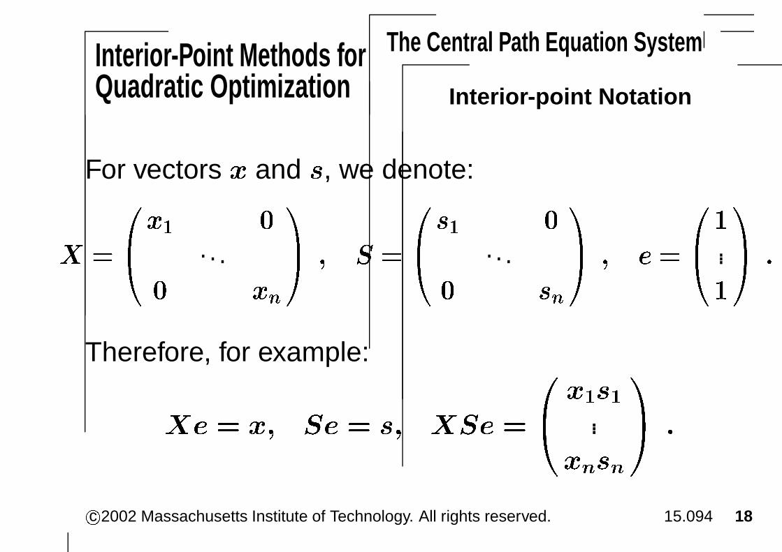
Interior-point Notation
For vectors � and , we denote:
� ��
��� �. . .
� ���
� � � ��
� � �
. . .
� ��
� � � ��
��
...
��
� �
Therefore, for example:
�� � �� �� � � ��� ��
� ���
...
����
� �
c�2002 Massachusetts Institute of Technology. All rights reserved. 15.094 18

Interior-Point Methods forQuadratic Optimization
The Central Path Equation System
The KKT conditions in IPM notation
The KKT optimality conditions:
�� � � � � �
���� ���� � � � � �
���� � � � � � � � ��
With our interior-point notation we can write this system as:
�� � � � � �
���� ���� � � � � �
��� � � �
c�2002 Massachusetts Institute of Technology. All rights reserved. 15.094 19

Interior-Point Methods forQuadratic Optimization
The Central Path Equation System
Relaxing the KKT Conditions
The KKT conditions are: �� � �� � � �
���� ��� � �� � �
��� � � �
We relax the KKT conditions by picking a value of � � � and instead solve:
�� � �� � � �
���� ��� � �� � �
��� � �� �
A solution ��� �� � � ���� ��� �� to this system for some value � is called apoint on the central path or central trajectory of the problem.
Proposition 3: If ��� �� � is on the central path for some value � � �, thenthe duality gap is
������� �����
�����
������
� �� � �� �
c�2002 Massachusetts Institute of Technology. All rights reserved. 15.094 20

Interior-Point Methods forQuadratic Optimization
The Central Path Equation System
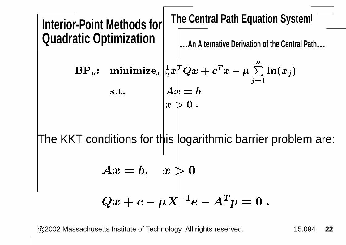
An Alternative Derivation of the Central Path...
Considering the following logarithmic barrier problemassociated with QP for a given value of �:
���� ����������
����� ���� �
�� ������
��� �� � �
� � � �
c�2002 Massachusetts Institute of Technology. All rights reserved. 15.094 21
Interior-Point Methods forQuadratic Optimization
The Central Path Equation System
...An Alternative Derivation of the Central Path...
��� �� �������
������ ���� �
������ ����
���� �� � �
� � � �
The KKT conditions for this logarithmic barrier problem are:
�� � �� � � �
�� �� �������� � � �
c�2002 Massachusetts Institute of Technology. All rights reserved. 15.094 22

Interior-Point Methods forQuadratic Optimization
The Central Path Equation System
...An Alternative Derivation of the Central Path
The KKT conditions for the logarithmic barrier problem:
�� � � � � �
��� �� ��������� � � �
Define �� ����� � � and rearrange the abovesystem, we obtain:
�� � �� � � �
�� ��� � �
��� � �� �
c�2002 Massachusetts Institute of Technology. All rights reserved. 15.094 23

Interior-Point Methods forQuadratic Optimization
The Newton Equation System
The current “point” is ���� � � � for which �� � � and
� � �, but ��� ��� and �� � ����� ���.
We are given a value of � � �.
We want to compute a direction ����� �� so that:
(1) ������ � �
(2) ������� ���� � ��� � �
(3) � �� �� � �� �� � � �� �c�2002 Massachusetts Institute of Technology. All rights reserved. 15.094 24
Interior-Point Methods forQuadratic Optimization
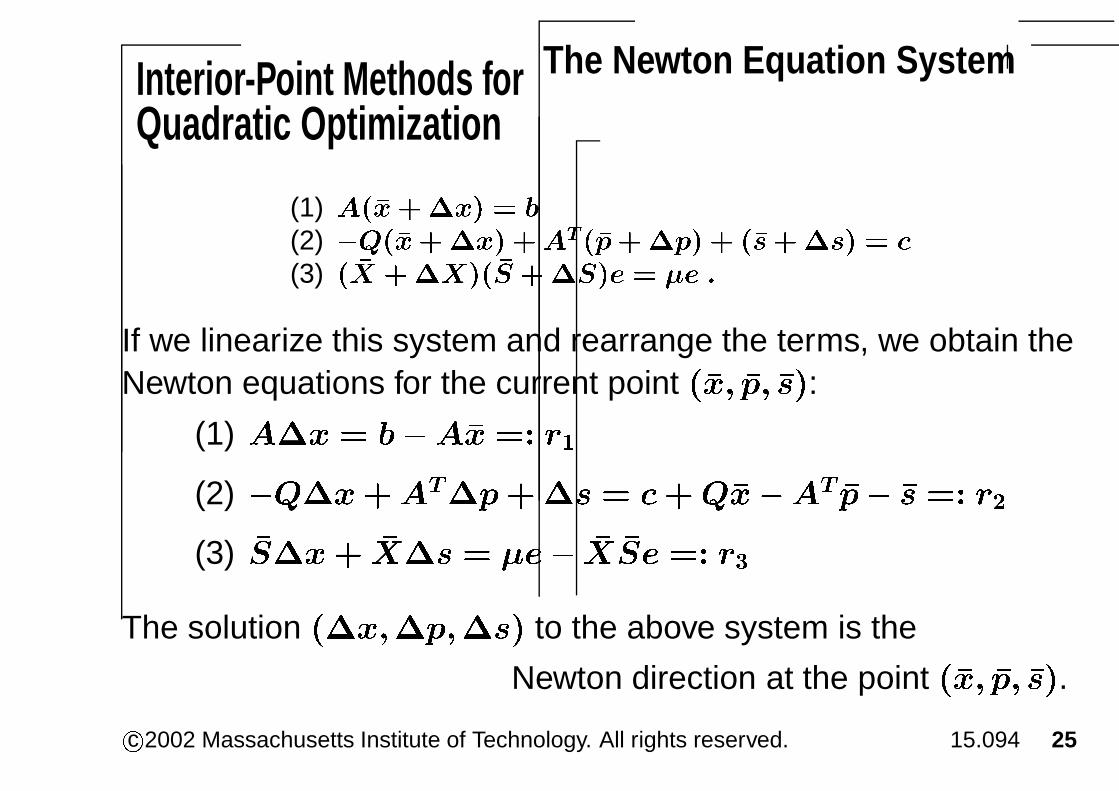
The Newton Equation System
(1) �������� � �
(2) ��������� ���������� � ����� � �
(3) � �� ����� �� ����� � �� �
If we linearize this system and rearrange the terms, we obtain theNewton equations for the current point ��� �� ���:
(1) ��� � ����� �� ��
(2) ������������ � �������� ��� �� �� ��
(3) ����� ���� � ��� �� ��� �� ��
The solution �������� to the above system is the
Newton direction at the point ��� �� ���.
c�2002 Massachusetts Institute of Technology. All rights reserved. 15.094 25
Interior-Point Methods forQuadratic Optimization
The Step-sizes
The Step...
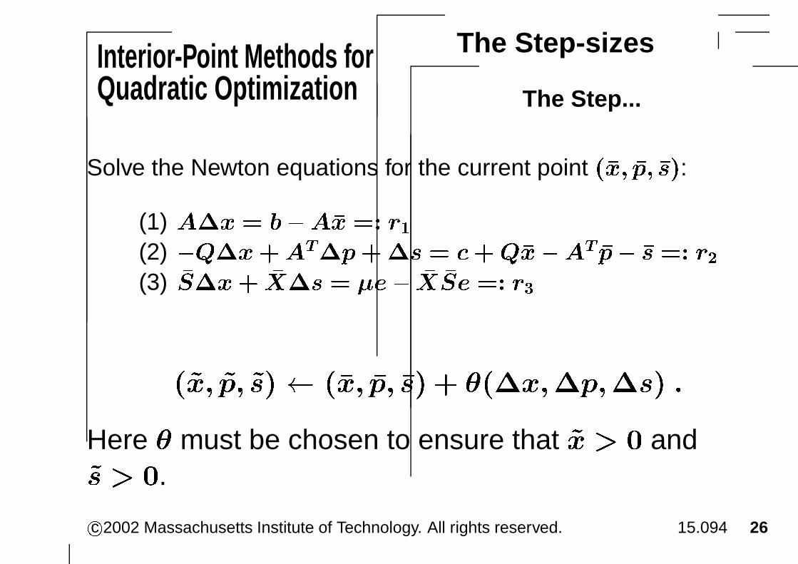
Solve the Newton equations for the current point ��� �� ���:
(1) ��� � ����� �� ��
(2) ������������ � �������� ��� �� �� ��
(3) ����� ���� � ��� �� ��� �� ��
���� � � � � ���� � � � ������ �� �
Here � must be chosen to ensure that �� � � and
� � �.
c�2002 Massachusetts Institute of Technology. All rights reserved. 15.094 26

Interior-Point Methods forQuadratic Optimization
The Step-sizes
...The Step
��� �� ��� � ��� �� ��� � ��������� �
To ensure that �� � � and � � �,we set � � � (� � ���� is typical), and set:
�� � ����
�� � ���
������
��
���
�� � ����
�� � ���
�����
�
��
� � ������ � ��� �
c�2002 Massachusetts Institute of Technology. All rights reserved. 15.094 27

Interior-Point Methods forQuadratic Optimization
Decreasing the Path Parameter �
We want to shrink � at each iteration, in order to (hopefully) shrink the dualitygap.
The current iterate is ���� ��� ��, and the current values satisfy:��� � � �� equivalently: � ���� �
�
�
Re-set � to��
��
����
��� ��
��
where “��” is user-specified.
Then solve: (1) ��� � ����� �� ��
(2) ����������� � �������� ��� � �� ��
(3) ����� ��� � ��� �� ��� �� ��c�2002 Massachusetts Institute of Technology. All rights reserved. 15.094 28

Interior-Point Methods forQuadratic Optimization
The Full Interior-Point Algorithm
a) Given ���� ��� �� satisfying �� � �, � � �, and �� � �, and � satisfying
� � � � �, and � � �. Set �� �.
b) Test stopping criterion. Check if: (1) ��� � �� � �
(2) � ��� ���� � � �� � �
(3) ���� � � �
If so, STOP. If not, proceed.
c) Set ���
���
������ ��
�
�d) Solve the Newton equation system:
(1) ��� � ���� �� ��
(2) ����������� � ���� ���� � �� ��
(3) ������ � ������ �� ��c�2002 Massachusetts Institute of Technology. All rights reserved. 15.094 29
Interior-Point Methods forQuadratic Optimization
The Full Interior-Point Algorithm
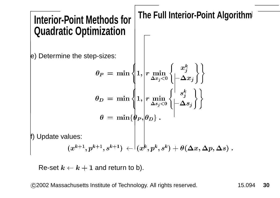
e) Determine the step-sizes:
� � ���
�� � ���
�����
��
����
�� � ���
�� � ���
�����
�
���
� � ����� � ��� �
f) Update values:
����� ���� ��� � ��� �� � � ���������� �
Re-set �� �� � and return to b).
c�2002 Massachusetts Institute of Technology. All rights reserved. 15.094 30

Interior-Point Methods forQuadratic Optimization
Solving the Newton Equations
(1) ��� � ����� �� ��
(2) ����������� � �������� ��� � �� ��
(3) ����� ��� � ��� �� ��� �� ��
After much manipulation, we obtain the following system andformula for ��:
������ ����� ������ � ������ ����� � ���� � ���
� ��
�� ��
������ ����� ������� �
������ ����� � ���� � ���
� ���
�
After computing ��, compute �� and �� as follows:
�� ������ ����� �
�� � ����� �������
�� � ���� �� ����� �
c�2002 Massachusetts Institute of Technology. All rights reserved. 15.094 31
Interior-Point Methods forQuadratic Optimization
Solving the Newton Equations
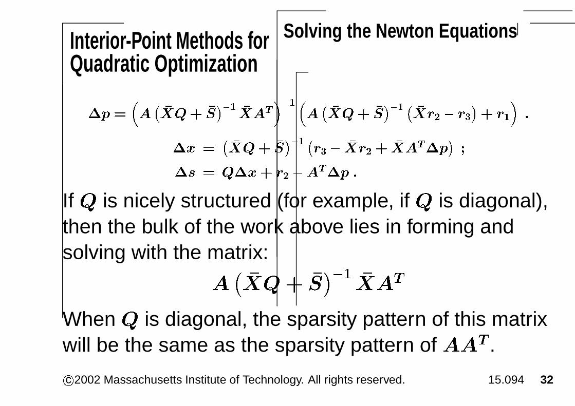
�� ��
������ �� �� ������� �
������ �� �� � ���� � ��
� ���
�
�� �
����� �� �� �
�� � ����� ������
�
� � ���� �� ����� �
If � is nicely structured (for example, if � is diagonal),then the bulk of the work above lies in forming andsolving with the matrix:
���� ����� ����
When � is diagonal, the sparsity pattern of this matrixwill be the same as the sparsity pattern of ��� .
c�2002 Massachusetts Institute of Technology. All rights reserved. 15.094 32

Interior-Point Methods forQuadratic Optimization
Remarks on Interior-Point Methods� The algorithm just described is almost exactly what is used in
commercial interior-point method software.
� The interior-point code LOQO, which is used in this course, isan implementation of this basic interior-point method, withsome additional enhancements.
� A typical interior-point code will solve a linear or quadraticoptimization problem in 25–80 iterations, regardless of thedimension of the problem.
c�2002 Massachusetts Institute of Technology. All rights reserved. 15.094 33
Interior-Point Methods forQuadratic Optimization
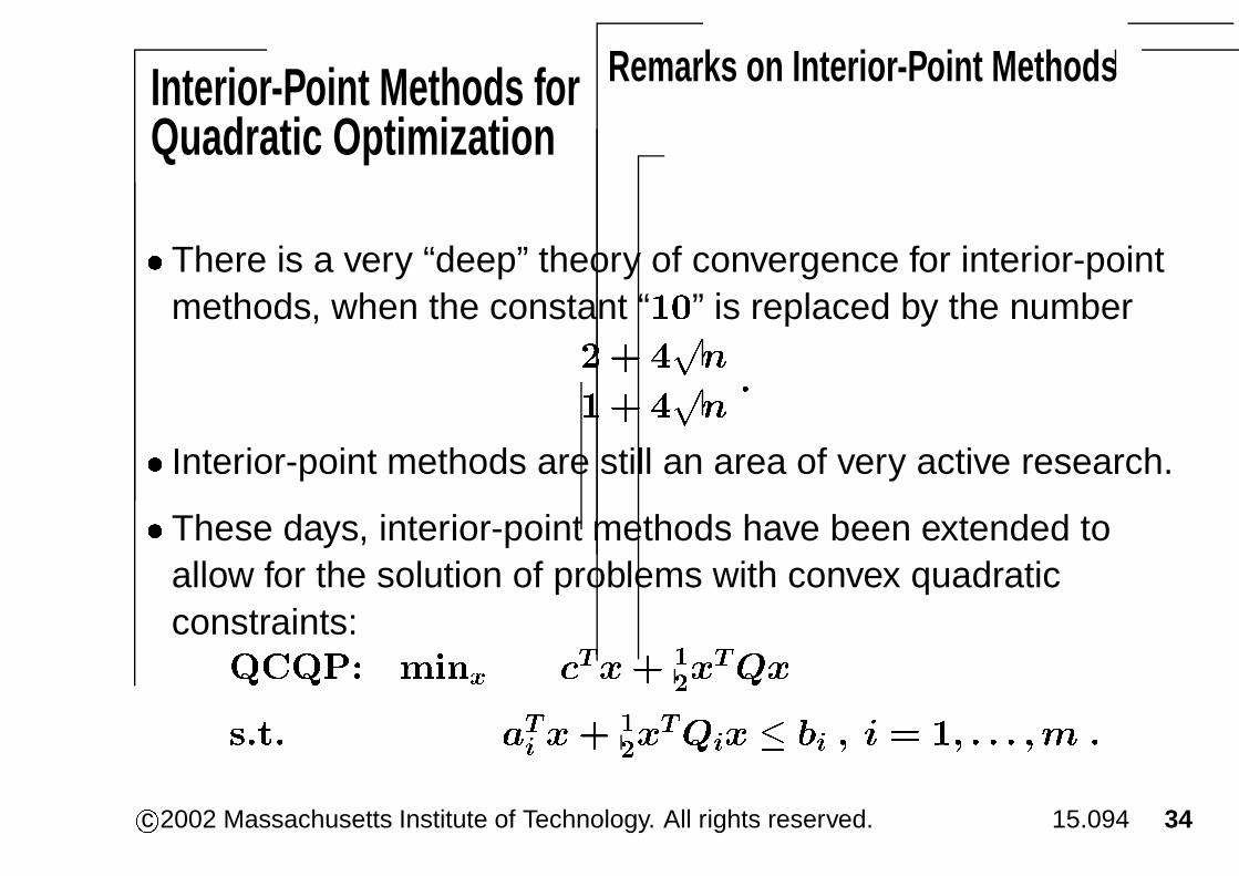
Remarks on Interior-Point Methods� There is a very “deep” theory of convergence for interior-point
methods, when the constant “��” is replaced by the number
�� ��
�
�� ��
��
� Interior-point methods are still an area of very active research.
� These days, interior-point methods have been extended toallow for the solution of problems with convex quadraticconstraints:
�� �� � ���� ������
���� ��� ���
������ � �� � � � � � � �
c�2002 Massachusetts Institute of Technology. All rights reserved. 15.094 34

Active Set Methods forQuadratic Optimization
Motivation
In a constrained optimization problem, someconstraints will be inactive at the optimal solution, andso can be ignored, and some constraints will be activeat the optimal solution.
If we knew which constraints were in which category,we could throw away the inactive constraints, and wecould reduce the dimension of the problem bymaintaining the active constraints at equality.
c�2002 Massachusetts Institute of Technology. All rights reserved. 15.094 35

Active Set Methods forQuadratic Optimization
Motivation
Of course, in practice, we typically do not know whichconstraints might be active or inactive at the optimalsolution.
Active set methods are designed to make an intelligentguess of the active set of constraints, and to modifythis guess at each iteration.
Herein we describe a relatively simple active-setmethod that can be used to solve quadraticoptimization problems.c�2002 Massachusetts Institute of Technology. All rights reserved. 15.094 36

Active Set Methods forQuadratic Optimization
Motivation
Consider a quadratic optimization problem in theformat:
��� ����������
����� ���
��� �� � �
� � � �
Suppose that � is very large.
Suppose that intuition suggests that very few variables
� will be non-zero at the optimal solution.
c�2002 Massachusetts Institute of Technology. All rights reserved. 15.094 37

Active Set Methods forQuadratic Optimization
Motivation
��� ��������
������ ���
�� � �� � �
� � � �
Suppose we have a feasible solution �.
Partition the components of �: � � ��� ���
where �� � � and �� � � �
In this partition, the number of elements in � is presumably smallrelative to �.
Re-write the data for our problem as:
� ��
��� ���
��� ����
� � ��� ��� � ��
����
�
c�2002 Massachusetts Institute of Technology. All rights reserved. 15.094 38

Active Set Methods forQuadratic Optimization
Motivation
We have a feasible solution � � �� � ���
where � � � and �� � � �
Re-write the data for our problem as:
� ��
� � �
�� ����
� � � �� ��� � � ��
� ��
��
“Guess” that the variables ��� � will be zero in the optimal solution, and socan be eliminated.
We then solve the much smaller problem:
�� � �� � ���������
���� � � � �� �
�� � � � � �
� � � �
c�2002 Massachusetts Institute of Technology. All rights reserved. 15.094 39
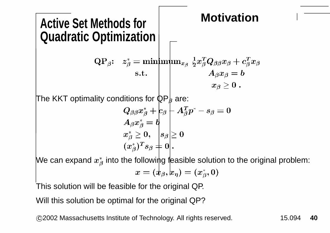
Active Set Methods forQuadratic Optimization
Motivation
�� � �� � ���������
���� � � � �� �
�� � � � � �
� � � �
The KKT optimality conditions for QP are:
� ��
� � ��� �� � � �
� ��
� �
�� � �� � �
��� �� � � �
We can expand �� into the following feasible solution to the original problem:
� � �� � ��� � ��� ���
This solution will be feasible for the original QP.
Will this solution be optimal for the original QP?
c�2002 Massachusetts Institute of Technology. All rights reserved. 15.094 40

Active Set Methods forQuadratic Optimization
Motivation
KKT conditions for QP : � ��
� � ��� �� � � �
� ��
� �
�� � �� � �
��� �� � � �
KKT conditions for QP stated with �� � ��� ��� and ��:�� � �
�� �����
�� �
���
� ��
���
��
���
��� ��
�
�� �
�� ����
�� �
�� �
��� ��� � �
��� �� � �� ��� � � �
All of these conditions are automatically satisfied except for the condition that
� � �, where: � �� �� ��
� �� ������ �
c�2002 Massachusetts Institute of Technology. All rights reserved. 15.094 41

Active Set Methods forQuadratic Optimization
Checking for Optimality
KKT conditions for QP stated with �� � ������ and ��:���� ���
��� �����
����
��
����
��
���
���
��� ��
����
� �
��� ����
����
� �
������ � �
�������� � � ���� � � �
�� �� �����
�� �� ������ �
Proposition 4: If � � �, then �� �� is an optimalsolution to QP.c�2002 Massachusetts Institute of Technology. All rights reserved. 15.094 42
Active Set Methods forQuadratic Optimization
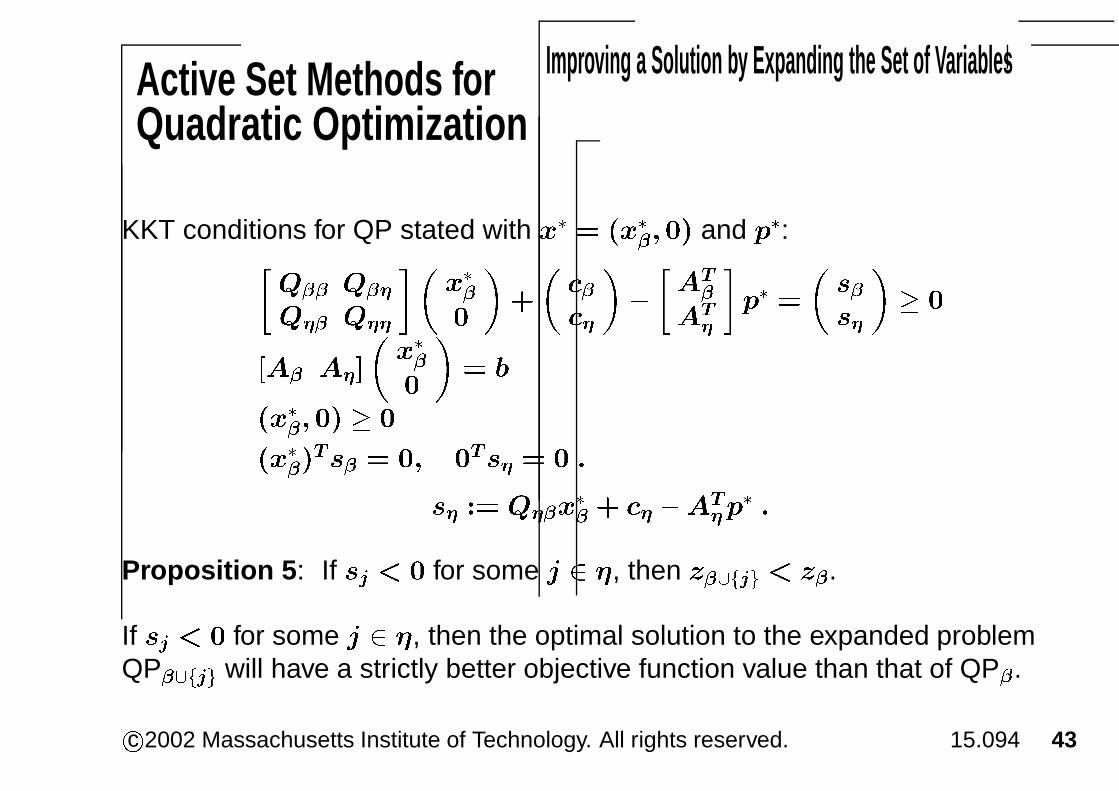
Improving a Solution by Expanding the Set of Variables
KKT conditions for QP stated with �� � ��� ��� and ��:�� � �
�� �����
�� �
���
� ��
���
��
���
��� ��
�
�� �
�� ����
�� �
�� �
��� ��� � �
��� �� � �� ��� � � �
� �� �� ��
� �� ������ �
Proposition 5: If � � � for some �, then � ���� � � .
If � � � for some �, then the optimal solution to the expanded problemQP ���� will have a strictly better objective function value than that of QP .
c�2002 Massachusetts Institute of Technology. All rights reserved. 15.094 43

Active Set Methods forQuadratic Optimization
An Active Set Algorithm
0. Define some partition of the indices, ��� � � � � �� � � �.
1. Solve the reduced problem�� � �� � ���������
���� � � � �� �
�� � � � � �
� � � �
obtaining the optimal solution �� and optimal KKT multiplier �� on theequations “� � � �”.
2. Compute � �� �� ��
� �� ������ �
If � � �, STOP. In this case, ��� ��� is optimal for QP. Otherwise if � � �
for some �, then set � � � �, � �� � � � �, and go to 1.
c�2002 Massachusetts Institute of Technology. All rights reserved. 15.094 44
Active Set Methods forQuadratic Optimization
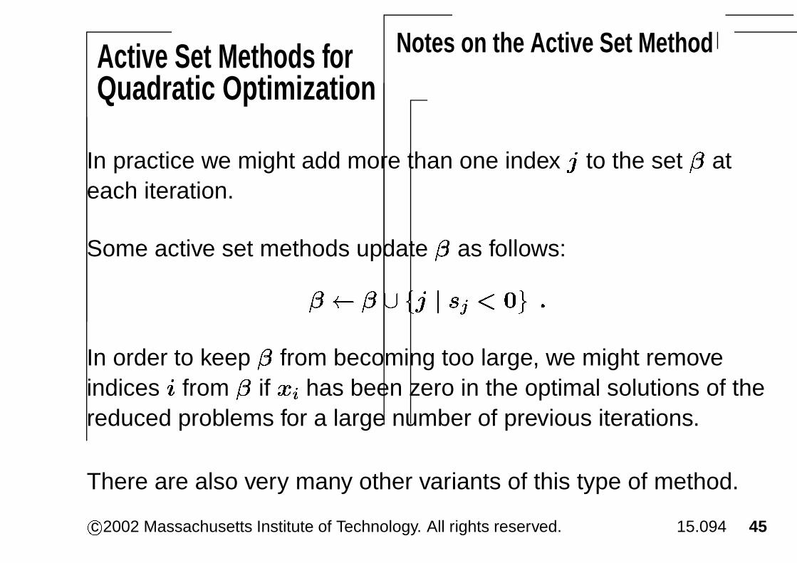
Notes on the Active Set Method
In practice we might add more than one index to the set � ateach iteration.
Some active set methods update � as follows:
� � � � � �� � � �
In order to keep � from becoming too large, we might removeindices from � if �� has been zero in the optimal solutions of thereduced problems for a large number of previous iterations.
There are also very many other variants of this type of method.
c�2002 Massachusetts Institute of Technology. All rights reserved. 15.094 45

Reduced Gradient Algorithmfor Nonlinear Optimization
Format for the Reduced Gradient Algorithm
The reduced gradient algorithm is designed to solve aproblem of the form:
���� ��������� ���
��� �� � �
� � � �
In the case of a suitably formatted quadratic problem,
��� ��
����� ��� and ���� � �� � �
c�2002 Massachusetts Institute of Technology. All rights reserved. 15.094 46

Reduced Gradient Algorithmfor Nonlinear Optimization
Assumptions Needed for Analysis
��� �� ������ ����
���� �� � �
� � � �
We assume the following regarding bases for thesystem “�� � �� � � �”:
�For any basis � � ��� � � � � �� with � ��, � isnonsingular.
�For any basic feasible solution �� � �� � ���� ���
we have � � �, where here � �� ��� � � � � �� �.
c�2002 Massachusetts Institute of Technology. All rights reserved. 15.094 47

Reduced Gradient Algorithmfor Nonlinear Optimization
Motivation for the Reduced Gradient Algorithm
Choose a Basis and Partition the Indices
��� �� ������ ����
���� �� � �
� � � �
The reduced gradient algorithm tries to mimic certain aspects ofthe simplex algorithm, starting with a partition of variables:
At any iteration, we have a feasible solution �� for NLP.
Pick a basis � for which ��� � �.
Such a basis must exist by our assumptions.
Such a basis might not be uniquely determined by the currentsolution ��.
Set � �� �� � � � � � �.
c�2002 Massachusetts Institute of Technology. All rights reserved. 15.094 48
Reduced Gradient Algorithmfor Nonlinear Optimization
Motivation for the Reduced Gradient Algorithm
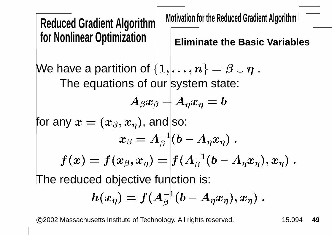
Eliminate the Basic Variables
We have a partition of ��� � � � � �� � � � � .The equations of our system state:
� � ���� � �
for any � � �� � �� , and so:� � ��� ������� �
��� � ��� � �� � ����� ������� � �� �
The reduced objective function is:
���� � ����� ������� � �� �
c�2002 Massachusetts Institute of Technology. All rights reserved. 15.094 49

Reduced Gradient Algorithmfor Nonlinear Optimization
Motivation for the Reduced Gradient Algorithm
The Reduced Gradient
The reduced objective function is:
���� � ����� ������� � �� �
The reduced gradient has the following formula:
����� � �������
������� � ��
�������
�� ����
������� � �� �
At �� � ��� � ��� , this is:
������ � ������ �������
�� ��� �
c�2002 Massachusetts Institute of Technology. All rights reserved. 15.094 50

Reduced Gradient Algorithmfor Nonlinear Optimization
Motivation for the Reduced Gradient Algorithm
A Direction Based on the Reduced Gradient
At �� � ���� ����, the reduced gradient is:
������� � ��������������
� ������� �
For notational convenience, let us use:
�� � ��� � ������� � ��������������
� �������
We use the reduced gradient to define a new direction � as follows:For �, we define:
�� ����
� ���� if ��� � �
���� if ��� � �
� if ��� � � and ��� � �
For �, we define: �� �� ����� ���� �
c�2002 Massachusetts Institute of Technology. All rights reserved. 15.094 51

Reduced Gradient Algorithmfor Nonlinear Optimization
Properties of the Reduced Gradient Direction
The following properties of the direction � are easy to prove:
�� is a feasible direction: �� � � and ���� � � forall � � � and sufficiently small.
� If � � �, then �� is a KKT point, with associated KKTmultipliers � � ���
�� ��� for the equations“�� � �”.
� If � �� �, then � is a descent direction, that is,
����� �� � �.
c�2002 Massachusetts Institute of Technology. All rights reserved. 15.094 52

Reduced Gradient Algorithmfor Nonlinear Optimization
The Reduced Gradient Algorithm
0. The current point is ��. Choose � for which �� � � and
� ��. Define � �� �� � � � � � �.
1. Compute the reduced gradient:
��� �� ��������������
� ������� �
2. Compute the direction �.
For �, define: �� ����
� ���� if ��� � �
���� if ��� � �
� if ��� � �� and ��� � �
For �, define: �� �� ����� ���� �
c�2002 Massachusetts Institute of Technology. All rights reserved. 15.094 53

Reduced Gradient Algorithmfor Nonlinear Optimization
The Reduced Gradient Algorithm
3. Compute the step-size. Define the following threequantities:
�� �� ��� ������� � ��
�� �� ��� ������� � � ��
�� �� ������!�
������ � � ������� ���
4. Update values. If � � �, then STOP (�� is a KKTpoint). If � �� �, then set ��� �����, and go to(0.).
c�2002 Massachusetts Institute of Technology. All rights reserved. 15.094 54

Reduced Gradient Algorithmfor Nonlinear Optimization
Comments on the Reduced Gradient Algorithm�The reduced gradient algorithm has been very
effective on problems with linear equality andinequality constraints. That is because it is actuallymimicking the simplex algorithm as much aspossible.
�One very useful modification of the reduced gradientalgorithm is to set � to correspond to the index of theset of the � largest components of ��.
c�2002 Massachusetts Institute of Technology. All rights reserved. 15.094 55

Reduced Gradient Algorithmfor Nonlinear Optimization
Comments on the Reduced Gradient Algorithm�As it turns out, there is no proof of convergence for
the algorithm as written above. A slightly modifiedrule for determining the direction � is given in thenotes, and leads to a straightforward proof ofconvergence.
c�2002 Massachusetts Institute of Technology. All rights reserved. 15.094 56

Some ComputationalResults
Problem Instances
REGULAR Model
We consider solving the dual of the pattern classificationquadratic program, namely D1:
��� ����� ����
��������
����� � � ��
���
������� ���
��� ���
�� ���
������� ���
��� ���
�
����
�����
�� ���
��� � � �
� � � � �
� �� �� �
We refer to this problem as the REGULAR model.
c�2002 Massachusetts Institute of Technology. All rights reserved. 15.094 57

Some ComputationalResults
Problem Instances
EXPANDED Model
Define the extra variables �: � ���
����"�#� �
�����$����
�
Re-write the REGULAR model as:
��� ������������
����"��
�����$� ��
����
�� � ���
����"�#� �
�����$����
� �
����"� �
�����$� � �
" � �� $ � �
" � $ � �
We refer to this model as the EXPANDED model.
c�2002 Massachusetts Institute of Technology. All rights reserved. 15.094 58

Some ComputationalResults
Problem Instances
REGULAR and EXPANDED Models
��� ����������
����"��
�����$� ��
��
����"�#� �
�����$����� �
����"�#� �
�����$����
�� �
����"� �
�����$� � �
" � �� $ � � " � $ � �
��� ������������
����"��
�����$� ��
����
�� � ���
����"�#� �
�����$����
� �
����"� �
�����$� � �
" � �� $ � � " � $ � �
c�2002 Massachusetts Institute of Technology. All rights reserved. 15.094 59

Some ComputationalResults
Ten Problem Instances
Ten instances of the pattern classification problemSeparable or Not Dimension � Number of points �
Separable 2 100Non-separable 2 100Separable 2 1,000Non-separable 2 1,000Separable 20 300Non-separable 20 300Separable 20 1,000Non-separable 20 1,000Separable 20 10,000Non-separable 20 10,000
c�2002 Massachusetts Institute of Technology. All rights reserved. 15.094 60

Some ComputationalResults
Ten Problem Instances
Separable 2-Dimensional Model
−1 −0.8 −0.6 −0.4 −0.2 0 0.2 0.4 0.6 0.8 1−1
−0.8
−0.6
−0.4
−0.2
0
0.2
0.4
0.6
0.8
1
Separable model with 100 points.
c�2002 Massachusetts Institute of Technology. All rights reserved. 15.094 61

Some ComputationalResults
Ten Problem Instances
Non-separable 2-Dimensional Model
−1 −0.8 −0.6 −0.4 −0.2 0 0.2 0.4 0.6 0.8 1−1
−0.8
−0.6
−0.4
−0.2
0
0.2
0.4
0.6
0.8
1
Non-separable model with 100 points.
c�2002 Massachusetts Institute of Technology. All rights reserved. 15.094 62

Some ComputationalResults
Ten Problem Instances
Separable 2-Dimensional Model
−1 −0.8 −0.6 −0.4 −0.2 0 0.2 0.4 0.6 0.8 1−1
−0.8
−0.6
−0.4
−0.2
0
0.2
0.4
0.6
0.8
1
Separable model with 1,000 points.
c�2002 Massachusetts Institute of Technology. All rights reserved. 15.094 63

Some ComputationalResults
Ten Problem Instances
Non-separable 2-Dimensional Model
−1 −0.8 −0.6 −0.4 −0.2 0 0.2 0.4 0.6 0.8 1−1
−0.8
−0.6
−0.4
−0.2
0
0.2
0.4
0.6
0.8
1
Non-separable model with 1,000 points.
c�2002 Massachusetts Institute of Technology. All rights reserved. 15.094 64

Some ComputationalResults
Algorithms Used
� IPM (Interior-Point Method) We solved the problems using the softwarecode LOQO, which is an interior-point algorithm implementation for linear,quadratic, and nonlinear optimization.
� MINOS We solved the problems using the software code MINOS, whichcombines aspects of the reduced gradient algorithm, quasi-Newtonmethods, etc. MINOS is best thought of as a solver for problems with linearconstraints and a quadratic, nonlinear, and/or linear objective function.
� ACTSET (Active Set Method) We solved the problems using a simpleactive set method, that adds one new index at each outer iteration, and doesnot drop any indices from consideration. The method starts with 30 indicesin the set .
c�2002 Massachusetts Institute of Technology. All rights reserved. 15.094 65

Some ComputationalResults
Algorithms Used
The Advantages of Active Set Methods
We should expect active set methods to perform verywell for this problem. Why?
�We expect very few points to be binding in the primalsolution.
�Therefore very few of the dual variables �� and/or ��
will be non-zero in the dual solution.
�And we are solving the dual.
c�2002 Massachusetts Institute of Technology. All rights reserved. 15.094 66

Some ComputationalResults
Objective Function Values
Optimal solution values reported by each method for each problem.REGULAR EXPANDED
ACTSETType � � IPM MINOS IPM MINOS IPM MINOSSep. 2 100 19.4941 19.4941 19.4941 19.4941 19.4941 19.4941Non. 2 100 992.4144 992.4144 992.4144 992.4144 992.4144 992.4144Sep. 2 1,000 88.8831 88.8831 88.8831 88.8831Non. 2 1,000 5,751.2161 5,751.2163 5,751.2161 5,751.2163Sep. 20 300 1.1398 1.1398 1.1398 1.1398 1.1398 1.1398Non. 20 300 2,101.6155 2,101.6155 2,101.6155 2,101.6155 2,101.6155 2,101.6155Sep. 20 1,000 1.9110 1.9111 1.9110 1.9111Non. 20 1,000 7,024.1791 7,024.1792 7,024.1791 7,024.1792Sep. 20 10,000 4.0165 4.0165 4.0165Non. 20 10,000 96,850.5000
Blanks indicate the method ran out of memory.
c�2002 Massachusetts Institute of Technology. All rights reserved. 15.094 67

Some ComputationalResults
Iterations of the Algorithms
Iteration count for each problem and each method.REGULAR EXPANDED
ACTSETType � � IPM MINOS IPM MINOS IPM MINOSSep. 2 100 27 110 26 9 58 17Non. 2 100 32 103 32 55 194 116Sep. 2 1,000 28 20 101 42Non. 2 1,000 60 335 1,237 1,019Sep. 20 300 30 353 32 88 340 319Non. 20 300 40 433 39 400 778 1,615Sep. 20 1,000 35 122 417 347Non. 20 1,000 54 1,888 2,022 5,753Sep. 20 10,000 173 598 372Non. 20 10,000 � 5,000 � 20,000 � 160,561Blanks indicate the method ran out of memory.
c�2002 Massachusetts Institute of Technology. All rights reserved. 15.094 68
Some ComputationalResults
Iterations of the Algorithms� The non-separable problems take more iterations to solve.
� Interior point methods use very few iterations in general, ascompared to MINOS.
� As the dimensions of the problem grows, the iteration count forMINOS grows proportionally.
� The iteration counts for interior-point method does not reallygrow much at all.
� The exception to these observations is the active setalgorithms, for which the total iteration count can be misleading.
c�2002 Massachusetts Institute of Technology. All rights reserved. 15.094 69

Some ComputationalResults
CPU Times for Each Algorithm
CPU times, in seconds.REGULAR EXPANDED
ACTSETType � � IPM MINOS IPM MINOS IPM MINOSSep. 2 100 2.89 51.92 0.20 0.13 0.04 0.20Non. 2 100 3.23 51.73 0.24 0.07 0.17 0.95Sep. 2 1,000 240.85 3.52 0.09 0.83Non. 2 1,000 278.56 3.60 3.39 13.64Sep. 20 300 27.16 914.10 8.04 1.90 0.99 6.63Non. 20 300 41.39 912.47 4.30 1.93 3.90 19.20Sep. 20 1,000 175.60 16.95 1.27 17.53Non. 20 1,000 289.15 17.17 12.00 99.19Sep. 20 10,000 1,805.75 1.02 166.20Non. 20 10,000 � 1,807.07 � 58,759 � 11,048.78Blanks indicate the method ran out of memory.
c�2002 Massachusetts Institute of Technology. All rights reserved. 15.094 70

Some ComputationalResults
Comparing REGULAR to EXPANDED
CPU times, in seconds.REGULAR EXPANDED
Type � � IPM MINOS IPM MINOSSep. 2 100 2.89 51.92 0.20 0.13Non. 2 100 3.23 51.73 0.24 0.07Sep. 2 1,000 240.85 3.52Non. 2 1,000 278.56 3.60Sep. 20 300 27.16 914.10 8.04 1.90Non. 20 300 41.39 912.47 4.30 1.93Sep. 20 1,000 175.60 16.95Non. 20 1,000 289.15 17.17Sep. 20 10,000 1,805.75Non. 20 10,000 � 1,807.07
Blanks indicate the method ran out of memory.
c�2002 Massachusetts Institute of Technology. All rights reserved. 15.094 71

Some ComputationalResults
Comparing REGULAR to EXPANDED�The interior-point algorithm takes much less time to
solve the REGULAR model.
�MINOS takes less time to solve the EXPANDEDmodel.
�The EXPANDED model takes less time to solve thandoes the REGULAR model.
�As the dimensions of the problem grows, the time tosolve the models grows, with one exception.
c�2002 Massachusetts Institute of Technology. All rights reserved. 15.094 72

Some ComputationalResults
Analysis of Active Set Method
CPU times, in seconds.EXPANDED EXPANDED
ACTSETType � � IPM MINOS IPM MINOSSep. 2 100 0.20 0.13 0.04 0.20Non. 2 100 0.24 0.07 0.17 0.95Sep. 2 1,000 240.85 3.52 0.09 0.83Non. 2 1,000 278.56 3.60 3.39 13.64Sep. 20 300 8.04 1.90 0.99 6.63Non. 20 300 4.30 1.93 3.90 19.20Sep. 20 1,000 175.60 16.95 1.27 17.53Non. 20 1,000 289.15 17.17 12.00 99.19Sep. 20 10,000 1,805.75 1.02 166.20Non. 20 10,000 � 1,807.07 � 58,759 � 11,048.78Blanks indicate the method ran out of memory.
c�2002 Massachusetts Institute of Technology. All rights reserved. 15.094 73

Some ComputationalResults
Analysis of Active Set Method�The active set method is not a clear winner when the
inner iterations are performed by MINOS.
�The active set method works very well when theinner iterations are performed by an interior-pointalgorithm. This seems to be the best combination.
c�2002 Massachusetts Institute of Technology. All rights reserved. 15.094 74