solute injection

7/27/2019 Solute Injection

http://slidepdf.com/reader/full/solute-injection 1/10

© COPYRIGHT 2008. All right reserved. No part of this documentation may be photocopied or reproduced in

any form without prior written consent from COMSOL AB. COMSOL, COMSOL Multiphysics, COMSOL Reac-

tion Engineering Lab, and FEMLAB are registered trademarks of COMSOL AB. Other product or brand names

are trademarks or registered trademarks of their respective holders.

Solute InjectionSOLVED WITH COMSOL MULTIPHYSICS 3.5a

®



S O L U T E I N J E C T I O N | 1

S o l u t e I n j e c t i o n

Introduction

Predicting the transport of contaminants that move with subsurface fluids generally

means analyzing at least two physics. This model tracks a contaminant that enters an

at a point, such as an injection well or toxic spill, and spreads through the aquifer with

time. The model has an analytic solution developed by Wilson and Miller (Ref. 1),

which has been used to test several dedicated fluid flow and transport codes. The

particular problem in this model comes from the MT3DMS manual of Zheng and

Wang (Ref. 2).

The analysis models steady-state fluid flow and follows up with a transient

solute-transport simulation; it employs the Darcy’s Law application mode and the

Solute Transport application mode from the Earth Science Module. In COMSOL

Multiphysics it is straightforward to specify a fluid velocity without solving a flow

problem. This example solves for the velocities to demonstrate the mechanics of

coupling flow and transport simulations in one model file.

The example also shows how to use the solver settings for the combined steady-state

and transient solution. The instructions detail how to model a point source using the

point flux settings available in the Earth Science Module.

The first section in this discussion gives an overview of the problem. Next it gives the

equations and describes how the fluid flow and the solute transport application modeslink in COMSOL Multiphysics. Next come a few implementation details including a

table of model data. The results shown next then illustrate various postprocessing

options. The last section describes how to build the model using the COMSOL

Multiphysics graphical user interface.

Model Definition

In this example, there is regional flow from left to right across a 450 m-by-300 m

aquifer. The fluid moves at a Darcy velocity of 0.11 m/d. The aquifer has

homogeneous and isotropic material properties. A point source releases a small

amount of fluid into the aquifer at 1 m3/d, a release rate small enough for the flow

field to remain uniform. The injected fluid carries a nonreactive solute at a

concentration of 1000 ppm. The contaminant migrates by advection and dispersion




and never reaches a boundary. The aquifer is initially pristine with concentrations

everywhere equal to zero. The only source of contaminant is the injection, so flow

through the inlet has zero concentration. The period of interest is one year.

F L U I D F L O W

Darcy’s law describes the fluid flow in this problem. With the hydraulic-head

formulation, the governing equation is

where K is hydraulic conductivity (m/d), H is hydraulic head (m), and Qs is the volume flow rate of fluid per unit volume of aquifer (d−1).

The point source is

where W is the volumetric pumping rate W (m3/d); b is the aquifer thickness (m); and

δ denotes the Dirac delta function, which is nonzero only in the point ( xi, yi), where xi and yi are the well coordinates.

Because the flow field is at steady state, you can obtain a unique solution by specifying

the model geometry, the point source, the material properties, and the boundary

conditions. The problem statement gives the hydraulic head at the inlet and the outlet

and indicates symmetry conditions on the sides. In the Darcy’s Law application mode,

you express these boundary conditions as

where n is the unit vector normal to the boundary.

C O U P L I N G

The groundwater-flow and solute-transport equations given here are linked by the

Darcy velocity, , which gives the specific flux (m/d) of fluid across an

infinitesimal surface representing both the solids and the pore spaces. COMSOL

Multiphysics computes the Darcy velocity vector u, which consists of the x and y

directional velocities denoted by u and v, respectively.

∇ K ∇ H –( )⋅ Qs

=

Qs

W

b-----δ x xi y yi–,–( )=

n K ∇ H ( )⋅ 0= ∂Ω Sides

H H in

= ∂Ω Inlet

H 0= ∂Ω Outlet

u K ∇ H –=




S O L U T E T R A N S P O R T

The advection-dispersion equation governs solute transport in this problem:

Here D L is the hydrodynamic dispersion tensor (m2/d); θs denotes the fluid volume

fraction; c gives the dissolved concentration (kg/m3); u is the Darcy velocity (m/d);

and Sc represents the quantity of solute added per unit volume of porous medium per

unit time (kg/(m3·d)).

The entries for the dispersion tensor are

where D Lii are the principal components of the dispersion tensor; D Lij are the cross

terms; α represents the dispersivity (m); and the subscripts “1” and “2” denote

longitudinal and transverse flow, respectively.

In this problem, Sc represents the solute injected at the point well, which is defined by

where cQ is the concentration of the solute in the water (kg/m3). You implement the

solute injection with the same logic as the fluid point source.

The problem statement specifies that the only contaminant source in the aquifer is the

point well, and that the boundaries far enough from the injection well for the

contaminant never to leave the model domain. You thus set the inlet concentration to

zero and assign the other boundaries an advective flux. The expressions for these

boundary conditions are

where n is the unit vector normal to the boundary.

θs

c∂

t∂----- ∇ θ

s– D L c uc+∇( )⋅+ S

c=

θ D Li i α1

ui2

u

------- α2

u j2

u

-------+=

θ D Li j θ D Lj i α1

α2

–( )uiu

j

u

-----------= =

Sc

Qs

cQW

b-----cQδ x xi y yi–,–( )= =

n θs

– D L c∇( )⋅ 0= ∂Ω Sides

c 0= ∂Ω Inlet

n θs

– D L c∇( )⋅ 0= ∂Ω Outlet




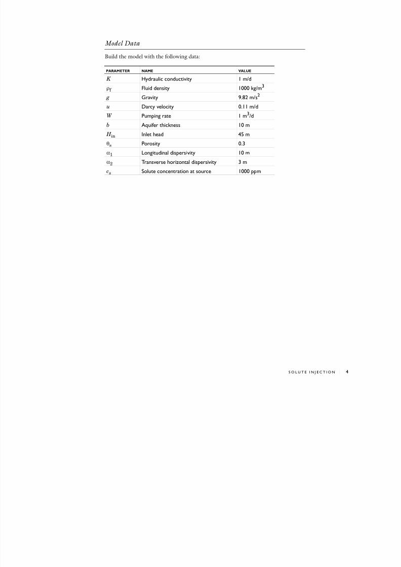
Model Data

Build the model with the following data:

PARAMETER NAME VALUE

K Hydraulic conductivity 1 m/d

ρf Fluid density 1000 kg/m3

g Gravity 9.82 m/s2

u Darcy velocity 0.11 m/d

W Pumping rate 1 m3/d

b Aquifer thickness 10 m

H in Inlet head 45 m

θs Porosity 0.3

α1 Longitudinal dispersivity 10 m

α2 Transverse horizontal dispersivity 3 m

cs Solute concentration at source 1000 ppm




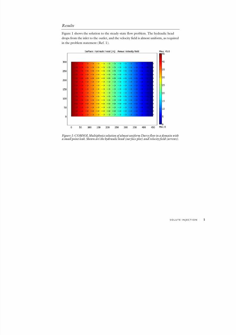
Results

Figure 1 shows the solution to the steady-state flow problem. The hydraulic headdrops from the inlet to the outlet, and the velocity field is almost uniform, as required

in the problem statement (Ref. 1).

Figure 1: COMSOL Multiphysics solution of almost uniform Darcy flow in a domain with a small point leak. Shown are the hydraulic head (surface plot) and velocity field (arrows).




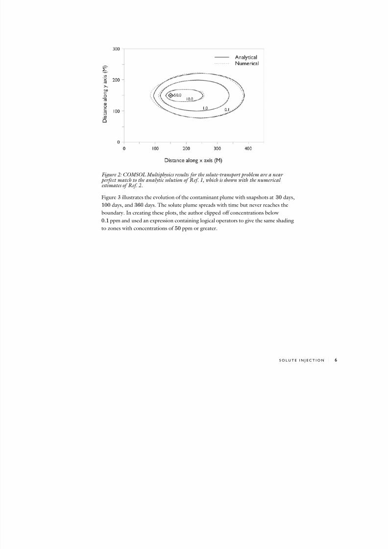
Figure 2: COMSOL Multiphysics results for th e solute-transport problem are a near perfect matc h to th e analytic solution of Ref. 1, which is shown with the numerical estimates of Ref. 2 .

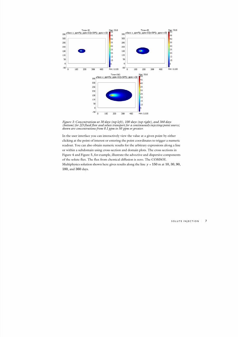
Figure 3 illustrates the evolution of the contaminant plume with snapshots at 30 days,

100 days, and 360 days. The solute plume spreads with time but never reaches the

boundary. In creating these plots, the author clipped off concentrations below

0.1 ppm and used an expression containing logical operators to give the same shading

to zones with concentrations of 50 ppm or greater.




Figure 3: Concentrations at 30 days (top left), 100 days (top right), and 360 days (bottom) for 2D fluid flow and solute transport for a continuously injecting point source; shown are concentrations from 0.1 ppm to 50 ppm or greater.

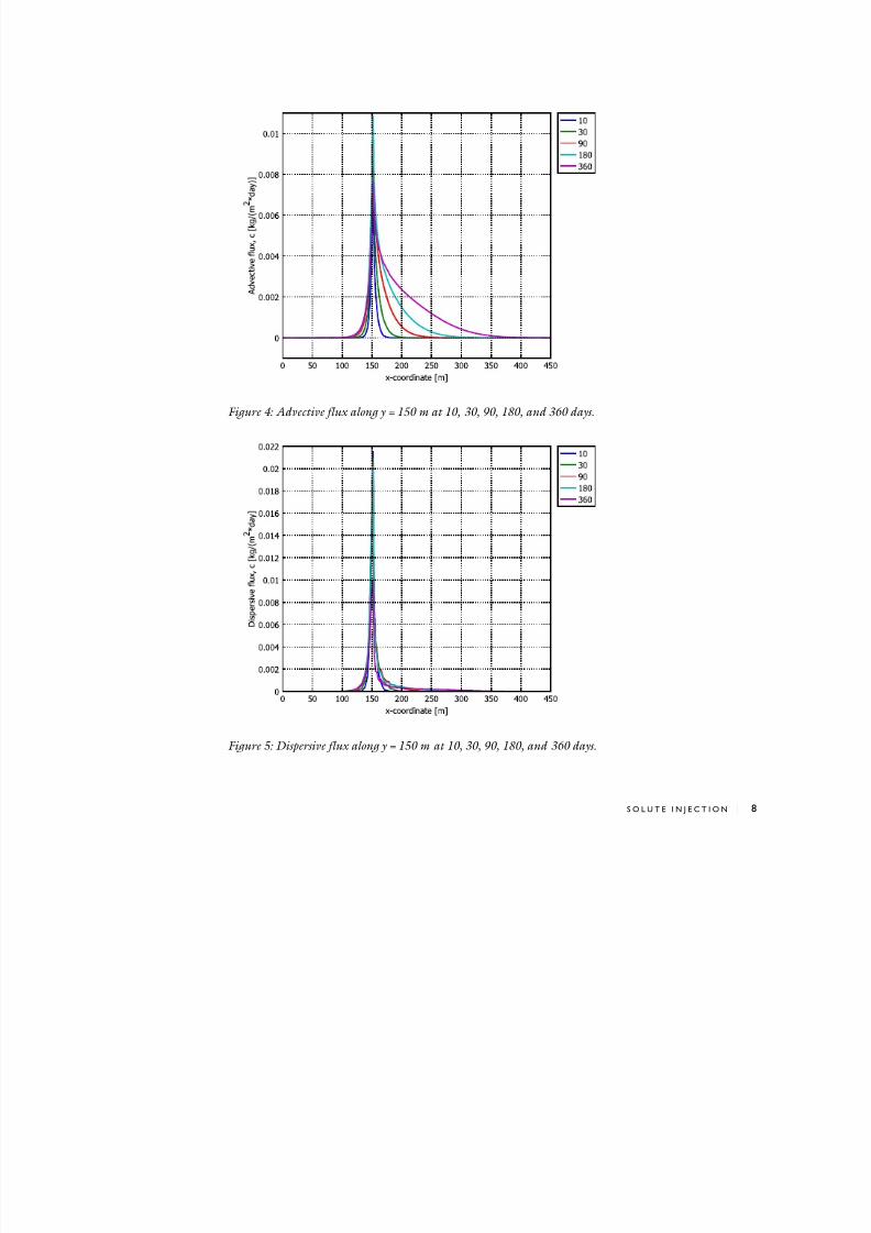
In the user interface you can interactively view the value at a given point by either

clicking at the point of interest or entering the point coordinates to trigger a numeric

readout. You can also obtain numeric results for the arbitrary expressions along a line

or within a subdomain using cross-section and domain plots. The cross sections in

Figure 4 and Figure 5, for example, illustrate the advective and dispersive components

of the solute flux. The flux from chemical diffusion is zero. The COMSOL

Multiphysics solution shown here gives results along the line y = 150 m at 10, 30, 90,

180, and 360 days.




Figure 4: Advective flux along y = 150 m at 10, 30, 90, 180, and 360 days.

Figure 5: Dispersive flux along y = 150 m at 10, 30, 90, 180, and 360 days.




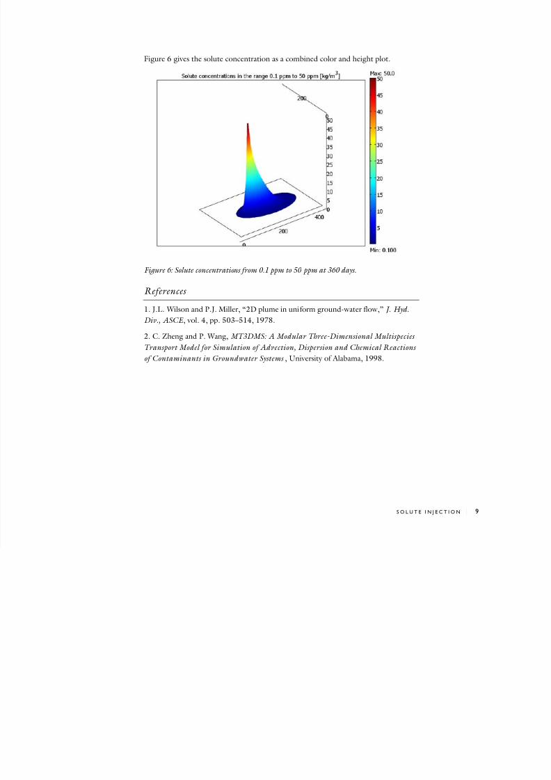
Figure 6 gives the solute concentration as a combined color and height plot.

Figure 6: Solute concentrations from 0.1 ppm to 50 ppm at 360 days.

References

1. J.L. Wilson and P.J. Miller, “2D plume in uniform ground-water flow,” J. Hyd.

Div., ASCE , vol. 4, pp. 503–514, 1978.

2. C. Zheng and P. Wang, MT3DMS: A Modular Three-Dimensional Multispecies

Transport Model for Simulation of Advection, Dispersion and Chemical Reactions

of Contaminants in Groundwater Systems , University of Alabama, 1998.

solute injection

Documents