solitons in aparametrically driven damped discrete ... · solitons in aparametrically driven damped...
TRANSCRIPT

arX
iv:1
206.
2405
v1 [
nlin
.PS]
11
Jun
2012
Solitons in a parametrically driven damped
discrete nonlinear Schrodinger equation
M. Syafwan1,2, H. Susanto1, and S. M. Cox1
1 School of Mathematical Sciences, University of Nottingham, University Park,Nottingham, NG7 2RD, UK
2 Department of Mathematics, Andalas University, Limau Manis, Padang, 25163,Indonesia
We consider a parametrically driven damped discrete nonlinear Schrodinger(PDDNLS) equation. Analytical and numerical calculations are performed todetermine the existence and stability of fundamental discrete bright solitons.We show that there are two types of onsite discrete soliton, namely onsitetype I and II. We also show that there are four types of intersite discretesoliton, called intersite type I, II, III, and IV, where the last two types areessentially the same, due to symmetry. Onsite and intersite type I solitons,which can be unstable in the case of no dissipation, are found to be stabilizedby the damping, whereas the other types are always unstable. Our furtheranalysis demonstrates that saddle-node and pitchfork (symmetry-breaking)bifurcations can occur. More interestingly, the onsite type I, intersite type I,and intersite type III-IV admit Hopf bifurcations from which emerge peri-odic solitons (limit cycles). The continuation of the limit cycles as well as thestability of the periodic solitons are computed through the numerical contin-uation software Matcont. We observe subcritical Hopf bifurcations along theexistence curve of the onsite type I and intersite type III-IV. Along the exis-tence curve of the intersite type I we observe both supercritical and subcriticalHopf bifurcations.
1 Introduction
In this paper, we consider a lattice model governed by a parametrically drivendamped discrete nonlinear Schrodinger (PDDNLS) equation
iφn = −ε∆2φn + Λφn + γφn − iαφn − σ|φn|2φn. (1)
In the above equation, φn ≡ φn(t) is a complex-valued wave function atsite n, the overdot and the overline indicate, respectively, the time derivativeand complex conjugation, ε represents the coupling constant between two

2 M. Syafwan, H. Susanto, and S. M. Cox
adjacent sites,∆2φn = φn+1−2φn+φn−1 is the one-dimensional (1D) discreteLaplacian, γ is the parametric driving coefficient with frequency Λ, α is thedamping constant, and σ is the nonlinearity coefficient. Here we confine ourstudy to the case of focusing nonlinearity, i.e., by setting positive valued σwhich then can be scaled, without loss of generality, to σ = +1.
In the absence of parametric driving and damping, i.e., for γ = 0 andα = 0, Eq. (1) reduces to the standard discrete nonlinear Schrodinger (DNLS)equation which appears in a wide range of important applications [1]. It isknown that the DNLS equation admits bright and dark solitons with focusingand defocusing nonlinearities, respectively. The stability of discrete brightsolitons in the DNLS system has been discussed, e.g., in Refs. [3, 4, 5], whereit was shown that one-excited-site (onsite) solitons are stable and two-excited-site (intersite) solitons are unstable, for any coupling constant ε. Moreover, thediscrete dark solitons in such a system have also been examined [6, 7, 8, 9, 10];it is known that intersite dark solitons are always unstable, for any ε, andonsite solitons are stable only in a small window of coupling constant ε.
Furthermore, the parametrically driven discrete nonlinear Schrodinger(PDNLS) equation, i.e, Eq. (1) with no damping (α = 0), has been stud-ied in [11] for the case of focusing nonlinearity, where it was reported that anonsite bright discrete soliton can be destabilized by a parametric driving. Thestudy of the same equation was extended for the other variants of discretesolitons in [12], showing that a parametric driving can not only destabilizeonsite bright solitons, but also stabilize intersite bright discrete solitons aswell as onsite and intersite dark discrete solitons. In the latter, the PDNLSmodel was particularly derived, using a multiscale expansion reduction, from aparametrically driven Klein-Gordon system describing coupled arrays of non-linear resonators in micro- and nano-electromechanical systems (MEMS andNEMS).
The discrete nonlinear Schrodinger equation with the inclusion of para-metric driving and damping terms as written in Eq. (1) was studied for thefirst time, to the best of our knowledge, by Hennig [22] focusing on the exis-tence and stability of localized solutions using a nonlinear map approach. Hedemonstrated that, depending upon the strength of the parametric driving,various types of localized lattice states emerge from the model, namely peri-odic, quasiperiodic, and chaotic breathers. The impact of damping constantand driving (but external) in the integrable version of the DNLS system, i.e.,the discrete Ablowitz-Ladik equation, has also been studied [23] which con-firmed the existence of breathers and multibreathers. In deriving Eq. (1), onecan follow, e.g., the method of reduction performed in [12] by including adamping term in the MEMS and NEMS resonators model.
On the other hand, the continuous version of the PDDNLS (1), i.e., whenφn ≈ φ and −ε∆2φn ≈ ∂2
xφ, was numerically discussed earlier in [24] result-ing in a single-soliton attractor chart on the (γ, α)-plane from which one maydetermine the regions of existence of stable stationary solitons as well as sta-ble time-periodic solitons (with period-1 and higher). Instead of using direct

Solitons in a parametrically driven damped DNLS equation 3
numerical integration as performed in the latter reference, Barashenkov andco-workers recently proposed obtaining the time-periodic one-soliton [25] andtwo-soliton [26] solutions as solutions of a two-dimensional boundary-valueproblem.
Our objective in the present paper is to examine the existence and sta-bility of the fundamental onsite and intersite excitations of bright solitons inthe focusing PDDNLS (1). The analysis of this model is performed througha perturbation theory for small ε which is then corroborated by numericalcalculations. Such analysis is based on the concept of the so-called anticon-tinuum (AC) limit approach which was introduced initially by MacKay andAubry [27]. In this approach, the trivial localized solutions in the uncoupledlimit ε = 0 are continued for weak coupling constant. Moreover, our study hereis also devoted to exploring the relevant bifurcations which occur in both sta-tionary onsite and intersite discrete solitons, including time-periodic solitonsemerging from Hopf bifurcations. For the latter scheme, we employ the nu-merical continuation software Matcont to path-follow limit cycles bifurcatingfrom the Hopf points.
The presentation of this paper is organized as follows. In Sec. 2, we firstlypresent our analytical setup for the considered model. In Sec. 3, we performthe existence and stability analysis of the discrete solitons through a pertur-bation method. Next, in Sec. 4, we compare our analytical results with thecorresponding numerical calculations and discuss bifurcations experienced bythe fundamental solitons. The time-periodic solitons appearing from the Hopfbifurcation points of the corresponding stationary solitons are furthermoreinvestigated in Sec. 5. Finally, we conclude our results in Sec. 6.
2 Analytical formulation
Static localized solutions of the focusing system (1) in the form of φn =un, where un is complex valued and time-independent, satisfy the stationaryequation
−ε∆2un + Λun + γun − iαun − |un|2un = 0, (2)
with spatial localization condition un → 0 as n → ±∞. We should notice thatEq. (2) (and accordingly Eq. (1)) admits the reflection symmetry under thetransformation
un → −un. (3)
Following [24, 25, 26], we assume that both the damping coefficient α andthe driving strength γ are positive. For the coupling constant ε, we also setit to be positive (the case ε < 0 can be obtained accordingly by the so-calledstaggering transformation un → (−1)nun and Λ → (Λ − 4ε)). The range ofthe parameter Λ is left to be determined later in the following discussion.
In the undriven and undamped cases, the localized solutions of Eq. (2) canbe chosen, without lack of generality, to be real-valued (with Λ > 0) [3]. This

4 M. Syafwan, H. Susanto, and S. M. Cox
is no longer the case for non-zero γ and α in the stationary PDDNLS (2),therefore we should always take into account complex-valued un. By writingun = an + ibn, where an, bn ∈ R, and decomposing the equation into real andimaginary parts, we obtain from Eq. (2) the following system of equations:
−ε∆2an + (Λ+ γ)an + αbn − (a2n + b2n)an = 0, (4a)
−ε∆2bn + (Λ− γ)bn − αan − (a2n + b2n)bn = 0. (4b)
Thus, the solutions of Eq. (2) can be sought through solving the above systemfor an and bn.
Next, to examine the stability of the obtained solutions, let us introducethe linearisation ansatz φn = un + δǫn, where δ ≪ 1. Substituting this ansatzinto Eq. (2) yields the following linearized equation at O(δ):
iǫn = −ε∆2ǫn + Λǫn + γǫn − iαǫn − 2|un|2ǫn − u2nǫn. (5)
By writing ǫn = ηneiωt + ξne
−iωt, Eq. (5) can be transformed into the eigen-value problem (EVP)
[
ε∆2 − Λ+ iα+ 2|un|2 u2n − γ
γ − u2n −ε∆2 + Λ− iα− 2|un|2
] [
ηnξn
]
= ω
[
ηnξn
]
. (6)
The stability of the solution un is then determined by the eigenvalues ω, i.e.,un is stable only when Im(ω) ≥ 0 for all eigenvalues ω.
As the EVP (6) is linear, we can eliminate one of the eigenvectors, forinstance ξn, so that we obtain the simplified form
[
L+(ε)L−(ε)− 4(anbn)2]
ηn = (ω − iα)2ηn, (7)
where the operators L+(ε) and L−(ε) are given by
L+(ε) ≡ −ε∆2 − (a2n + 3b2n − Λ+ γ),
L−(ε) ≡ −ε∆2 − (3a2n + b2n − Λ− γ).
3 Perturbation analysis
Solutions of Eq. (2) for small coupling constant ε can be calculated analyticallythrough a perturbative analysis, i.e., by expanding un in powers of ε as
un = u(0)n + εu(1)
n + ε2u(2)n + · · · . (8)
Solutions un = u(0)n correspond to the case of the uncoupled limit ε = 0.
For this case, Eq. (2) permits the exact solutions u(0)n = a
(0)n + ib
(0)n in which
(
a(0)n , b
(0)n
)
can take one of the following values
Solitons in a parametrically driven damped DNLS equation 5
(0, 0), (sA+,−sB−), (sA−,−sB+), (9)
where
A± =
√
(γ ±√
γ2 − α2)(Λ ±√
γ2 − α2)
2γ,
B± =
√
(γ ±√
γ2 − α2)(Λ ∓√
γ2 − α2)
2γ,
and s = ±1. Due to the reflection symmetry (3), we are allowed to restrictconsideration to the case s = +1.
Following the assumption γ, α > 0, we can easily confirm that nonzero(A+,−B−) and (A−,−B+) are together defined in the following range ofparameters
Λ > γ ≥ α > 0. (10)
In particular, when γ = α, the values of (A+,−B−) are exactly the same as(A−,−B+).
Once a configuration for u(0)n is determined, its continuation for small ε can
be sought by substituting expansion (8) into Eq. (2). In this paper, we onlyfocus on two fundamental localized solutions, i.e., one-excited site (onsite) andin-phase two-excited site (intersite) bright solitons. Out-of-phase two-excitedsite modes also referred to as twisted discrete solitons (see, e.g., [28]), whichexist in the model considered herein, are left as a topic of future research.
Next, to study the stability of the solitons, we also expand the eigenvectorhaving component ηn and the eigenvalue ω in powers of ε as
ηn = η(0)n + εη(1)n +O(ε2), ω = ω(0) + εω(1) +O(ε2). (11)
Substituting these expansions into Eq. (7) and collecting coefficients at suc-cessive powers of ε yield the O(1) and O(ε) equations which are respectivelygiven by
Lη(0)n = 0, (12)
Lη(1)n = fn, (13)
where
L = L+(0)L−(0)− 4(a(0)n b(0)n )2 − (ω(0) − iα)2, (14)
fn =[
L−(0)(∆2 + 2a(0)n a(1)n + 6b(0)n b(1)n ) + L+(0)(∆2 + 2b(0)n b(1)n + 6a(0)n a(1)n )
+8a(0)n b(0)n (a(0)n b(1)n + a(1)n b(0)n ) + 2ω(0)ω(1) − 2iαω(1)]
η(0)n . (15)
One can check that the operator L is self-adjoint and thus the eigenvector
h = col(..., η(0)n−1, η
(0)n , η
(0)n+1, ...) is in the null-space of the adjoint of L.
6 M. Syafwan, H. Susanto, and S. M. Cox
From Eq. (12), we obtain that the eigenvalues in the uncoupled limit ε = 0are
ω(0)C = ±
√
Λ2 − γ2 + iα, (16)
and
ω(0)E = ±
√
L+(0)L−(0)− 4(a(0)n b
(0)n )2 + iα, (17)
which correspond, respectively, to the solutions u(0)n = 0 (for all n) and
u(0)n = a
(0)n + ib
(0)n 6= 0 (for all n). For bright soliton solutions having boundary
condition un → 0 as n → ±∞, the eigenvalues ω(0)E and ω
(0)C have, respec-
tively, finite and infinite multiplicities which then generate a correspondingdiscrete and continuous spectrum as ε is turned on.
Let us first investigate the significance of the continuous spectrum. Byintroducing a plane-wave expansion ηn = µeiκn + νe−iκn, one can obtain thedispersion relation
ω = ±√
(2ε(cosκ− 1)− Λ)2 − γ2 + iα, (18)
from which we conclude that the continuous band lies between
ωL = ±√
Λ2 − γ2 + iα, when κ = 0, (19)
andωU = ±
√
Λ2 − γ2 + 8ε(Λ+ 2ε) + iα, when κ = π, (20)
From the condition (10), one can check that all the eigenvalues ω ∈ ±[ωL, ωU ]always lie on the axis Im(ω) = α > 0 for all ε, which means that the continuousspectrum does not give contribution to the instability of the soliton. Therefore,the analysis of stability is only devoted to the discrete eigenvalues. Discreteeigenvalues that potentially lead to instability are also referred to as criticaleigenvalues.
3.1 Onsite bright solitons
When ε = 0, the configuration of an onsite bright soliton is of the form
u(0)n = 0 for n 6= 0, u
(0)0 = A+ iB, (21)
where (A,B) 6= (0, 0). From the combination of nonzero solutions (9), we canclassify the onsite bright solitons, indicated by the different values of (A,B),as follows:
(i) Type I, which has (A,B) = (A+,−B−),(ii) Type II, which has (A,B) = (A−,−B+),
Solitons in a parametrically driven damped DNLS equation 7
which we denote hereinafter by un{±} and un{∓}, respectively.The continuation of the above solutions for small ε can be calculated from
the expansion (8), from which one can show that an onsite soliton type I andtype II, up to O(ε2), are respectively given by
un{±} =
(A+ − iB−) +(A+−iB
−)ε
Λ+√
γ2−α2, n = 0,
(A+−iB−)ε
Λ+√
γ2−α2, n = −1, 1,
0, otherwise,
(22)
and
un{∓} =
(A− − iB+) +(A
−−iB+)ε
Λ−√
γ2−α2, n = 0,
(A−−iB+)ε
Λ−√
γ2−α2, n = −1, 1,
0, otherwise.
(23)
In particular, when α = γ, the onsite type I and type II become exactly thesame.
To examine the stability of the solitons, we need to calculate the corre-sponding discrete eigenvalues for each of type I and type II, which we elaboratesuccessively.
3.1.1 Onsite type I
One can show from Eq. (12) that at ε = 0, an onsite bright soliton type I hasa leading-order discrete eigenvalue which comes as the pair
ω(0){±} = ±
√P + iα, (24)
whereP = 4Λ
√
γ2 − α2 + 4γ2 − 5α2. (25)
The eigenvector corresponding to the above eigenvalue has components η(0)n =
0 for n 6= 0 and η(0)0 = 1.
We notice that P can be either positive or negative depending on whetherα ≶ αth, where
αth =2
5
√
5γ2 − 2Λ2 + Λ√
4Λ2 + 5γ2. (26)
Therefore, the eigenvalue ω(0){±} can be either
ω1(0){±} = ±
√
4Λ√
γ2 − α2 + 4γ2 − 5α2 + iα, (27)
for the case α < αth, or
ω2(0){±} = i
(
α±√
5α2 − 4Λ√
γ2 − α2 − 4γ2
)
, (28)

8 M. Syafwan, H. Susanto, and S. M. Cox
for the case αth < α ≤ γ.The continuation of the eigenvalues (29) and (30) for nonzero ε can be
evaluated from Eq. (13) by applying a Fredholm solvability condition. As thecorresponding eigenvector has zero components except at site n = 0, we onlyneed to require f0 = 0, from which we obtain the discrete eigenvalue of un{±}
for small ε, up to O(ε2), as follows.
(i) For the case α < αth:
ω1{±} = ±√
4Λ√
γ2 − α2 + 4γ2 − 5α2± (4√
γ2 − α2)ε√
4Λ√
γ2 − α2 + 4γ2 − 5α2
+iα.
(29)(ii) For the case αth < α ≤ γ:
ω2{±} = i
α±√
5α2 − 4Λ√
γ2 − α2 − 4γ2 ∓ (4√
γ2 − α2)ε√
5α2 − 4Λ√
γ2 − α2 − 4γ2
.
(30)
We should note here that the above expansions remain valid if ±P are O(1).Let us now investigate the behavior of the above eigenvalue in each case. In
case (i), the imaginary part of ω1(0){±} (i.e., when ε = 0) is α, which is positive.
We also note that |ω1(0){±}| ≷ |ω(0)
C | when α ≶ αcp, where
αcp =1
5
√
25γ2 − Λ2. (31)
As ε increases, the value of |ω1{±}| also increases. As a result, the eigenvaluesω1{±} will collide either with the upper band (ωU ) of the continuous spec-trum for α < αcp, or with the lower band (ωL) for αcp < α < αth. Thesecollisions then create a corresponding pair of eigenvalues bifurcating from theaxis Im
(
ω1{±}
)
= α. This collision, however, does not immediately lead tothe instability of the soliton as it does for α = 0 [11, 12]. In addition, the
distance between ω1(0){±} and ω
(0)C increases as α tends to 0, which means that
the corresponding collisions for smaller α happen at larger ε. From the aboveanalysis we hence argue that for α < αth and for relatively small ε, the onsitesoliton type I is stable.
In case (ii), it is clear that√
5α2 − 4Λ√
γ2 − α2 − 4γ2 ≤ α which implies
0 ≤ min(Im(ω2(0){±})) < α; the latter indicates the soliton is stable at ε =
0. As ε increases, both max(Im(ω2{±})) and min(Im(ω2{±})) tend to α atwhich they finally collide. From this fact, we conclude that for small ε and forαth < α ≤ γ, the soliton remains stable. In particular, when α = γ, we havemin(Im(ω2{±})) = 0 for all ε, which then implies that the soliton is alwaysstable.

Solitons in a parametrically driven damped DNLS equation 9
3.1.2 Onsite type II
Performing the calculations as before, we obtain that the discrete eigenvalue(in pairs) of an onsite bright soliton type II is given, up to O(ε2), by
ω{∓} = i
α±√
4Λ√
γ2 − α2 − 4γ2 + 5α2 ± (4√
γ2 − α2)ε√
4Λ√
γ2 − α2 − 4γ2 + 5α2
.
(32)
Again, we should assume that the term (4Λ√
γ2 − α2 − 4γ2 + 5α2) in theabove expansion is O(1).
When α < γ, we simply have√
4Λ√
γ2 − α2 − 4γ2 + 5α2 > α, from which
we deduce min(Im(ω(0){∓})) < 0, meaning that at ε = 0 the soliton is unstable.
In fact, as ε increases, the value of min(Im(ω{∓})) decreases. Therefore, inthis case we infer that the soliton is unstable for all ε.
When α = γ, by contrast, the value of min(Im(ω{∓})) is zero for all ε,which indicates that the soliton is always stable. In fact, the stability of anonsite type II in this case is exactly the same as in type I. This is understand-able as the onsite type I and type II possess the same profile when α = γ.
3.2 Intersite bright solitons
Another natural fundamental solution to be studied is a two-excited site (in-tersite) bright soliton whose mode structure in the uncoupled limit is of theform
u(0)n =
A0 + iB0, n = 0,A1 + iB1, n = 1,0, otherwise,
(33)
where (A0, B0) 6= (0, 0) and (A1, B1) 6= (0.0). The combination of the nonzerosolutions (9) gives the classification for the intersite bright solitons, indicatedby different values of (A0, B0) and (A1, B1), as follows:
(i) Type I, which has (A0, B0) = (A1, B1) = (A+,−B−),(ii) Type II, which has (A0, B0) = (A1, B1) = (A−,−B+),(iii)Type III, which has (A0, B0) = (A+,−B−) and (A1, B1) = (A−,−B+),(iv)Type IV, which has (A0, B0) = (A−,−B+) and (A1, B1) = (A+,−B−).
Let us henceforth denote the respective types by un{±±}, un{∓∓}, un{±∓},and un{∓±}.
From the expansion (8), we obtain the continuation of each type of solutionfor small ε, which are given, up to order ε2, by

10 M. Syafwan, H. Susanto, and S. M. Cox
un{±±} =
(A+ − iB−) +12(A+−iB
−)ε
Λ+√
γ2−α2, n = 0,
(A+ − iB−) +12(A+−iB
−)ε
Λ+√
γ2−α2, n = 1,
(A+−iB−)ε
Λ+√
γ2−α2, n = −1, 2,
0, otherwise,
(34)
un{∓∓} =
(A− − iB+) +12
(A−−iB+)ε
Λ−√
γ2−α2, n = 0,
(A− − iB+) +12
(A−−iB+)ε
Λ−√
γ2−α2, n = 1,
(A−−iB+)ε
Λ−√
γ2−α2, n = −1, 2,
0, otherwise,
(35)
un{±∓} =
(A+−iB+)ε
Λ+√
γ2−α2, n = −1,
(A+ − iB−) +12
(A+−iB−)ε
γ(Λ+√
γ2−α2), n = 0,
(A− − iB+) +12
(A−−iB+)ε
γ(Λ−√
γ2−α2), n = 1,
(A−−iB
−)ε
Λ−√
γ2−α2, n = 2,
0, otherwise,
(36)
un{∓±} =
(A−−iB
−)ε
Λ−√
γ2−α2, n = −1,
(A− − iB+) +12
(A−−iB+)ε
γ(Λ−√
γ2−α2), n = 0,
(A+ − iB−) +12
(A+−iB−)ε
γ(Λ+√
γ2−α2), n = 1,
(A+−iB+)ε
Λ+√
γ2−α2, n = 2,
0, otherwise,
(37)
where
A± = 2γA± + (Λ ±√
γ2 − α2)A∓, (38)
B± = 2γB∓ − (Λ±√
γ2 − α2)B±. (39)
All solutions above are defined on the region (10) and exhibit the same profileswhen α = γ. One can check that intersite type III and IV are symmetric, thusthey should really be considered as one solution. However, we write them hereas two ‘different’ solutions because, as shown later in the next section, theyform two different branches in a pitchfork bifurcation (together with intersitetype I).
Let us now examine the stability of each solution by investigating theircorresponding discrete eigenvalues.
3.2.1 Intersite type I
By considering Eq. (12) and carrying out the same analysis as in onsite typeI, we obtain that the intersite type I has the double leading-order discrete

Solitons in a parametrically driven damped DNLS equation 11
eigenvalue
ω1(0){±±} = ±
√
4Λ√
γ2 − α2 + 4γ2 − 5α2 + iα, (40)
for α < αth, and
ω2(0){±±} = i
(
α±√
5α2 − 4Λ√
γ2 − α2 − 4γ2
)
, (41)
for αth < α ≤ γ. The corresponding eigenvector for the above eigenvalues has
components η(0)n = 0 for n 6= 0, 1, η
(0)0 6= 0, and η
(0)1 6= 0.
One can check, as in onsite type I, that the position of ω1(0){±±} relative to
ω(0)C depends on whether α ≶ αcp = 1
5
√
25γ2 − Λ2, i.e., the value of |ω1(0){±±}|
is greater (less) than |ω(0)C | when α is less (greater) than αcp.
The next correction for the discrete eigenvalues of an intersite type II canbe calculated from Eq. (13), for which we need a solvability condition. Due tothe presence of two non-zero components of the corresponding eigenvector atn = 0, 1, we only require f0 = 0 and f1 = 0. Our simple analysis then shows
η(0)0 = ±η
(0)1 from which we obtain that each of double eigenvalues (40) and
(41) bifurcates into two distinct eigenvalues, which are given, up to order ε2,as follows.
(i) For the case α < αth:
ω11{±±} = ±√
4Λ√
γ2 − α2 + 4γ2 − 5α2± (2√
γ2 − α2)ε√
4Λ√
γ2 − α2 + 4γ2 − 5α2
+iα,
(42)
ω12{±±} = ±√
4Λ√
γ2 − α2 + 4γ2 − 5α2∓ 2(Λ+√
γ2 − α2)ε√
4Λ√
γ2 − α2 + 4γ2 − 5α2
+iα.
(43)(ii) For the case αth < α ≤ γ:
ω21{±±} = i
α±√
5α2 − 4Λ√
γ2 − α2 − 4γ2 ∓ (2√
γ2 − α2)ε√
5α2 − 4Λ√
γ2 − α2 − 4γ2
,
(44)
ω22{±±} = i
α±√
5α2 − 4Λ√
γ2 − α2 − 4γ2 ± 2(Λ+√
γ2 − α2)ε√
5α2 − 4Λ√
γ2 − α2 − 4γ2
.
(45)
As before, we assume here that the terms ±(4Λ√
γ2 − α2 − 4γ2 + 5α2) areO(1) so that the above expansions remain valid.
Let us first observe the behavior of the eigenvalues in case (i). In the
uncoupled limit ε = 0, the imaginary part of ω11(0){±±} = ω12
(0){±±} is α >
12 M. Syafwan, H. Susanto, and S. M. Cox
0 which indicates that the soliton is initially stable. When ε is turned on,the value of |ω11{±±}| increases but |ω12{±±}| decreases. Therefore, we candetermine the mechanism of collision of these two eigenvalues with the inneror outer boundary of continuous spectrum (ωL or ωU ) as follows.
• For α < αcp, the first collision is between ω12{±±} and ωU . Because ωU
moves faster (as ε is varied) than ω11{±±}, the next collision is betweenthese two aforementioned eigenvalues.
• For α > αcp, the mechanism of collision can be either between ω12{±±}
and ωL, or between ω12{±±} and itself.
All of the mechanisms of collision above generate new corresponding pairsof eigenvalues bifurcating from their original imaginary parts, which is α.Yet these collisions do not immediately cause an instability, because α > 0.Therefore, we may conclude that for sufficiently small ε and for α < αth, anintersite bright soliton type I is stable.
Next, we describe the analysis for the eigenvalues in case (ii). When
ε = 0, we have 0 ≤ min(Im(ω21(0){±±})) = min(Im(ω22
(0){±±})) < α. As ε is
increased, min(Im(ω21{±±})) increases but min(Im(ω22{±±})) decreases. Thelatter then becomes negative, leading to the instability of soliton. By takingmin(Im(ω22{±±})) = 0, one obtains
εcr =α√
5α2 − 4Λ√
γ2 − α2 − 4γ2
2(Λ+√
γ2 − α2)− 5α2 − 4Λ
√
γ2 − α2 − 4γ2
2(Λ+√
γ2 − α2), (46)
which yields an approximate boundary for the onset of instability, e.g., in the(ε, α)-plane for fixed Λ and γ.
3.2.2 Intersite type II
From our analysis of Eqs. (12) and (13), we obtain the discrete eigenvaluesfor an intersite bright soliton type II, which are given, with errors of order ε2,by
ω1{∓∓} = i
α±√
4Λ√
γ2 − α2 − 4γ2 + 5α2 ± (2√
γ2 − α2)ε√
4Λ√
γ2 − α2 − 4γ2 + 5α2
,
(47)
ω2{∓∓} = i
α±√
4Λ√
γ2 − α2 − 4γ2 + 5α2 ± 2(Λ−√
γ2 − α2)ε√
4Λ√
γ2 − α2 − 4γ2 + 5α2
,
(48)
assuming the term (4Λ√
γ2 − α2 − 4γ2 + 5α2) is O(1). Notice that ω1{∓∓}
and ω2{∓∓} are equal when α =√
4γ2 − Λ2/2.
Solitons in a parametrically driven damped DNLS equation 13
When α < γ, both min(Im(ω1{∓∓})) and min(Im(ω2{∓∓})) are negative atε = 0 and always decrease as ε is increased; the decrement of min(Im(ω2{∓∓}))
is greater than min(Im(ω1{∓∓})) for α >√
4γ2 − Λ2/2. When α = γ,min(Im(ω1{∓∓})) and min(Im(ω2{∓∓})) are zero at ε = 0. At nonzero ε,the former remains zero, but the latter becomes negative and decreases as εincreases. These facts allow us to conclude that an intersite bright soliton typeII is always unstable, except at α = γ and ε = 0. One can check that whenα = γ, the eigenvalues of intersite type II are the same as in intersite type I.
3.2.3 Intersite type III and IV
As intersite type III and IV are symmetric, their eigenvalues are exactly thesame. Our calculation shows the following.
(i) For the case α < αth, the eigenvalues of the intersite type III and IV, upto O(ε2), are
ω11{±∓} = ω11{∓±} = iα±√
4Λ√
γ2 − α2 + 4γ2 − 5α2
± (2γ√
γ2 − α2 − Λγ + α√
Λ2 − γ2 + α2)ε
γ
√
4Λ√
γ2 − α2 + 4γ2 − 5α2
, (49)
ω12{±∓} = ω12{∓±} = i
(
α±√
4Λ√
γ2 − α2 − 4γ2 + 5α2
± (2γ√
γ2 − α2 + Λγ − α√
Λ2 − γ2 + α2)ε
γ√
4Λ√
γ2 − α2 − 4γ2 + 5α2
. (50)
(ii) For the case αth < α ≤ γ, the eigenvalues, up to order ε2, are
ω21{±∓} = ω21{∓±} = i
(
α±√
5α2 − 4Λ√
γ2 − α2 − 4γ2
∓ (2γ√
γ2 − α2 − Λγ + α√
Λ2 − γ2 + α2)ε
γ√
5α2 − 4Λ√
γ2 − α2 − 4γ2
, (51)
ω22{±∓} = ω22{∓±} = i
(
α±√
4Λ√
γ2 − α2 − 4γ2 + 5α2
± (2γ√
γ2 − α2 + Λγ − α√
Λ2 − γ2 + α2)ε
γ√
4Λ√
γ2 − α2 − 4γ2 + 5α2
. (52)
We should assume again that the terms ±(4Λ√
γ2 − α2 + 4γ2 − 5α2) and
(4Λ√
γ2 − α2 − 4γ2 + 5α2) in the above expansions are of O(1).

14 M. Syafwan, H. Susanto, and S. M. Cox
In the first case, the eigenvalues (50) are apparently pure imaginary, withan imaginary part whose minimum value is negative for all ε. In the secondcase, it is clear that for α < γ the minimum value of the imaginary partof the eigenvalues (51) is positive (less than α) initially at ε = 0 and thenincreases as ε increases. However, for this case (α < γ), the minimum valueof the imaginary part of the eigenvalues (52), which are exactly the same asthe eigenvalues (50), is negative at ε = 0 and then decreases as ε is turnedon. In contrast, for α = γ the minimum value of the imaginary part of theeigenvalues (51) and (52) remains zero for all ε. The above fact shows thatboth intersite soliton type III and IV are always unstable, except at α = γ.In fact, as shown in the numerical calculation later, the intersite type III andIV are no longer defined along this line, due to a pitchfork bifurcation withintersite type I.
4 Comparisons with numerical results, and bifurcations
In order to find the numerical solutions for each soliton discussed in theprevious section, we solve the stationary equation (2) [cf. Eq. (4)] usinga Newton-Raphson (NR) method. The evaluation is performed in domainn ∈ [−N,N ], i.e., for a lattice of 2N + 1 sites, with periodic boundary con-ditions u±(N+1) = u∓N . As an initial guess, we use the corresponding exactsoliton solutions in the uncoupled limit ε = 0 from which we then numericallycontinue for nonzero ε. As an illustrative example, the numerical solutionsfor each type of onsite and intersite bright soliton with parameter values(ε, Λ, γ, α) = (0.1, 1, 0.5, 0.1) are depicted in Fig. 1. The corresponding ana-lytical approximations are also plotted therein showing good agreement withthe numerical results.
To examine the stability of each soliton, we solve the eigenvalue problem(6) numerically and then compare the results with the analytical calculations.Moreover, we show later that the relevant solitons experience saddle-nodeand/or pitchfork bifurcations. To depict the diagram of these bifurcations, weuse a pseudo-arclength method which allows us to continue the solution pastturning points (by varying one parameter). In addition, our analysis of theeigenvalues for some particular solutions leads to the fact of the presence ofHopf bifurcations. We will determine the nature of Hopf bifurcation pointsand perform continuation of the bifurcating limit cycles in the next sectionby employing the numerical continuation package Matcont.
In all illustrative examples below, we use N = 50 which is large enough tocapture the behavior of the soliton in an infinite domain but not too costly innumerical computations. In addition, for the sake of simplicity, we set Λ = 1and γ = 0.5.

Solitons in a parametrically driven damped DNLS equation 15
−5 0 5−0.2
0
0.2
0.4
0.6
0.8
1
1.2
1.4
n
Re(
u n), Im
(un)
(a) Onsite type I
−5 0 5
−0.8
−0.6
−0.4
−0.2
0
0.2
n
Re(
u n), Im
(un)
(b) Onsite type II
−5 0 5−0.2
0
0.2
0.4
0.6
0.8
1
1.2
1.4
n
Re(
u n), Im
(un)
(c) Intersite type I
−5 0 5−0.8
−0.7
−0.6
−0.5
−0.4
−0.3
−0.2
−0.1
0
0.1
n
Re(
u n), Im
(un)
(d) Intersite type II
−5 0 5−1
−0.5
0
0.5
1
1.5
n
Re(
u n), Im
(un)
(e) Intersite type III
−5 0 5−1
−0.5
0
0.5
1
1.5
n
Re(
u n), Im
(un)
(f) Intersite type IV
Fig. 1. Profiles of onsite and intersite bright solitons of different types, as indicatedin the caption of each panel, for parameter values (ε,Λ, γ, α) = (0.1, 1, 0.5, 0.1). Solidlines show the numerical results while dashed lines indicate the analytical approxi-mations given by Eqs. (22) and (23) for the onsite type I and II, respectively, andby Eqs. (34), (35), (36), and (37) for the intersite type I, II, III, and IV, respec-tively. The circle and cross markers correspond to the real and imaginary part ofthe solutions, respectively.

16 M. Syafwan, H. Susanto, and S. M. Cox
4.1 Onsite bright solitons
4.1.1 Onsite type I
We start by testing the validity of our analytical approximation for the criticaleigenvalues given by Eqs. (29) and (30). We present in Fig. 2 comparisonsbetween the analytical and numerical results for the critical eigenvalues asfunctions of ε. We plot comparisons for three values α = 0.1, 0.47, 0.497 torepresent the cases α < αcp, αcp < α < αth, and αth < α < γ, respectively(see again the relevant discussion in the previous section). From the figure,we conclude that our prediction for small ε is relatively close to the numerics.
0 0.02 0.04 0.06 0.08 0.10.2
0.4
0.6
0.8
1
1.2
1.4
1.6
1.8
2
ε
|ω|
Fig. 2. Comparisons between the critical eigenvalues of an onsite bright solitontype I obtained numerically (solid lines) and analytically (dashed lines). The upperand middle curves correspond, respectively, to α = 0.1 and α = 0.485, which areapproximated by Eq. (29), whereas the lower corresponds to α = 0.497, which isapproximated by Eq. (30).
For the three values of α given above, we now present in Fig. 3 the eigen-value structure of the soliton and the corresponding diagram for the imaginarypart of the critical eigenvalues as functions of ε. Let us now describe the resultsin more detail.
First, we notice that at ε = 0 the critical eigenvalues for α = 0.1 lie be-yond the outer band of the continuous spectrum, while for α = 0.485 theyare trapped between the two inner bands of the continuous spectrum. As ε isturned on, the corresponding critical eigenvalues for α = 0.1 and α = 0.485collide with, respectively, the outer and the inner bands, leading to the bi-furcation of the corresponding eigenvalues. The minimum imaginary part ofthese bifurcating eigenvalues, however, does not immediately become negative.Hence, for relatively small ε we conclude that the soliton is always stable; thisin accordance with our analytical prediction of the previous section. The crit-ical values of ε at which min(Im(ω)) = 0 indicating the onset of the instability
Solitons in a parametrically driven damped DNLS equation 17
are depicted by the star markers in panels (c) and (f) in Fig. 3. Interestingly,for α = 0.485 there is a re-stabilization of the soliton as shown by the largerε star marker in panel (f).
Next, for α = 0.497 the discrete eigenvalues initially (at ε = 0) lie on theimaginary axis; they come in pairs and are symmetric about the line Im(ω) =α = 0.497, furthermore the minimum one is above the real axis. When εincreases, both eigenvalues approach one another and finally collide at thepoint (0, α = 0.497) creating a new pair of discrete eigenvalues along the lineIm(ω) = α = 0.497. Each pair of the eigenvalues then again bifurcates afterhitting the inner edge of the continuous spectrum. However, the minimumimaginary part of these bifurcating eigenvalues is always greater than zeroeven for larger ε [see panel (i)]. From this fact, we therefore conclude that thesoliton in this case is always stable. This conclusion agrees with our analyticalinvestigation.
The minimum value of Im(ω) (in color representation) of the onsite brightsoliton type I for a relatively large range of ε and α gives the (in)stabilityregion in the (ε, α)-plane as presented in Fig. 4. The stable region is indeeddetermined whenever min (Im(ω)) ≥ 0 for each ε and α. The lower and upperdotted horizontal lines in this figure, i.e., respectively, α = αcp ≈ 0.4583 andα = αth ≈ 0.49659, represent the boundaries of the regions which distinguishthe description of the eigenvalue structure of the soliton. The solid line in thisfigure indicates the (in)stability boundary, i.e., when min (Im(ω)) = 0. Threerepresentative points (star markers) lying on this line reconfirm the corre-sponding points in panels (c) and (f) in Fig. 3. As shown in the figure, thereis an interval of α in which the soliton is stable for all ε. This is interesting asthe onsite soliton, which was shown [11, 12] to be destabilized by a parametricdriving, now can be re-stabilized by a damping constant.
Let us revisit Fig. 3 for α = 0.1 and α = 0.485. We notice that at zero-crossing points εc (shown by the star markers in panels (c) and (f)), thefollowing conditions hold:
(i) There is a pair (equal and opposite) of non-zero real eigenvalues, and(ii) The ε-derivative of the imaginary part of the pair of eigenvalues mentioned
in (i) is non-zero at εc.
The second condition is also called the transversality condition. We assumethat the so-called first Lyapunov coefficient of the zero-crossing points isnonzero, i.e. the genericity condition. According to the Hopf bifurcation the-orem (see, e.g., Ref. [29], keeping in mind that our eigenvalue is denoted byiω), the above conditions imply that at ε = εc Eq. (1) has time-periodic (limitcycle) solutions bifurcating from a (steady-state) onsite bright soliton type I.We then call such a critical point εc a Hopf point. By applying the centremanifold theorem, for example, we can generally determine the nature of aHopf point εc through its first Lyapunov coefficient l1(εc) (see, e.g., Ref. [29]);the Hopf bifurcation is subcritical iff l1(εc) > 0 and supercritical iff l1(εc) < 0.

18 M. Syafwan, H. Susanto, and S. M. Cox
−4 −2 0 2 40
0.05
0.1
0.15
0.2
Re(ω)
Im(ω
)
(a) α = 0.1, ε = 0.1
−4 −2 0 2 4−0.2
−0.1
0
0.1
0.2
0.3
0.4
Re(ω)
Im(ω
)
(b) α = 0.1, ε = 0.5
0 0.5 1 1.5 2
−0.4
−0.2
0
0.2
0.4
0.6
ε
Im(ω
crit)
(c) α = 0.1
−3 −2 −1 0 1 2 30
0.2
0.4
0.6
0.8
1
Re(ω)
Im(ω
)
(d) α = 0.485, ε = 0.05
−3 −2 −1 0 1 2 3
0
0.2
0.4
0.6
0.8
1
Re(ω)
Im(ω
)
(e) α = 0.485, ε = 1.2
0 0.5 1 1.5 2
0
0.2
0.4
0.6
0.8
1
ε
Im(ω
crit)
(f) α = 0.485
−3 −2 −1 0 1 2 30
0.2
0.4
0.6
0.8
1
Re(ω)
Im(ω
)
(g) α = 0.497, ε = 0.02
−3 −2 −1 0 1 2 30
0.2
0.4
0.6
0.8
1
Re(ω)
Im(ω
)
(h) α = 0.497, ε = 1
0 0.5 1 1.5 20
0.2
0.4
0.6
0.8
1
ε
Im(ω
crit)
(i) α = 0.497
Fig. 3. The first and second columns of panels show the (Re(ω), Im(ω))-plane of theeigenvalues of onsite bright solitons type I for several values of α and ε, as indicatedin the caption of each panel (each row of panels depicts three different values of α).For α = 0.1 and α = 0.485, the corresponding left and middle panels illustrate theeigenvalues of stable and unstable solitons. The third column shows the path of theimaginary part of the critical eigenvalues ωcrit as functions of ε for the correspondingα. The locations of ε at which Im(ωcrit) = 0 are indicated by the star markers.
Because the occurrence of Hopf bifurcation in the onsite type I also in-dicates the onset of (in)stability, the collection of Hopf bifurcation points inthe (ε, α)-plane therefore lies precisely on the (in)stability boundary line (seeagain Fig. 4). However, at the stationary point ε ≈ 1.46 the condition (ii)for the occurrence of a (non-degenerate) Hopf bifurcation does not hold. Atthis special point, we have a saddle-node bifurcation of Hopf points, i.e. adouble-Hopf (Hopf-Hopf) bifurcation. Due to the violation of the transver-sality condition, there may be no periodic solution or even multiple periodicsolutions at the denegerate point. We will examine this point later in Sec. 5,where it will be shown through numerical continuations of limit cycles nearthe degenerate point that the former possibility occurs.

Solitons in a parametrically driven damped DNLS equation 19
ε
α
0 0.5 1 1.5 20
0.1
0.2
0.3
0.4
0 0.5 1 1.5 20.496
0.498
0.5
−0.6
−0.5
−0.4
−0.3
−0.2
−0.1
0
0.1
0.2
0.3
0.4
unstablestable
stable
Fig. 4. (Color online) The (in)stability region of onsite bright solitons type I in the(ε, α)-plane. The corresponding color represents the minimum value of Im(ω) (for alleigenvalues ω) for each ε and α. Thus, the region in which min (Im(ω)) ≥ 0 indicatesthe region of stable soliton, otherwise unstable. The boundary of stable-unstableregions, i.e., when min (Im(ω)) = 0, is given by the solid line (three representativepoints (star markers) on this line correspond to those points in panels (c) and (f)in Fig. 3). The boundary curve also indicates the occurrence of Hopf bifurcationswith one degenerate point, i.e. a double-Hopf bifurcation, at ε ≈ 1.46 as indicatedby the white-filled circle. The lower and upper horizontal dotted lines correspond toEqs. (31) and (26), respectively (see text).
4.1.2 Onsite type II
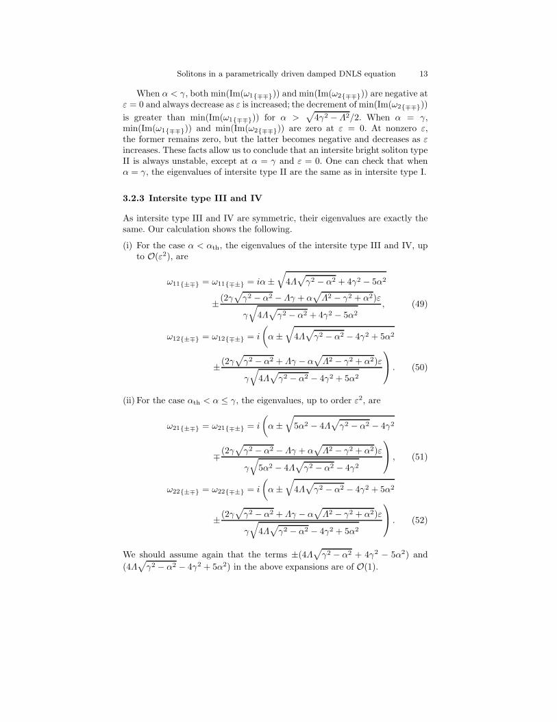
For this type of solution, a comparison between the critical eigenvalues ob-tained by analytical calculation, which is given by Eq. (32), and by numerics,is presented in Fig. 5. We conclude that our analytical prediction for small εis quite accurate.
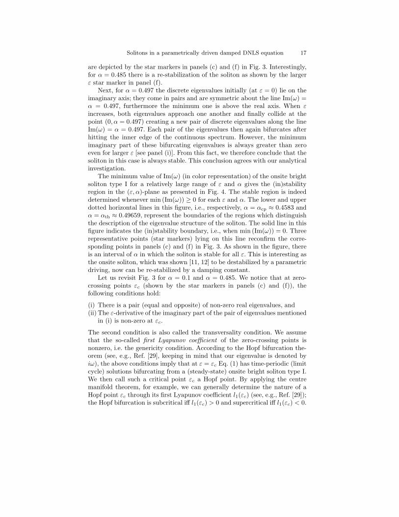
The eigenvalue structure of onsite solitons type II for α = 0.1 and the twovalues ε = 0.1, 1 and the corresponding curve of imaginary part of the criticaleigenvalues are given in Fig. 6. This figure shows that the soliton is alwaysunstable even for a large ε. This fact is consistent with the analytical predic-tion. We notice in the figure that there is a new pair of discrete eigenvaluesbifurcating from the inner edge of continuous spectrum at relatively large ε[see panel (b)].
By evaluating the minimum value of Im(ω) for a relatively large ε and α, weobtain that the soliton is always unstable for α < γ = 0.5 and, contrastingly,stable for α = γ. In the latter case, the eigenvalues of the onsite type II are
20 M. Syafwan, H. Susanto, and S. M. Cox
0 0.002 0.004 0.006 0.008 0.010.9
0.905
0.91
0.915
0.92
0.925
0.93
ε
|ω|
Fig. 5. Comparison between the critical eigenvalues of onsite bright solitons type IIfor α = 0.1 produced by numerics (solid line) and by analytical approximation (32)(dashed line).
−2 −1.5 −1 −0.5 0 0.5 1 1.5 2
−1
−0.5
0
0.5
1
Re(ω)
Im(ω
)
(a) α = 0.1, ε = 0.01
−2 −1.5 −1 −0.5 0 0.5 1 1.5 2−1.5
−1
−0.5
0
0.5
1
1.5
Re(ω)
Im(ω
)
(b) α = 0.1, ε = 1
0 0.5 1 1.5−1.5
−1
−0.5
0
0.5
1
1.5
ε
Im(ω
crit)
(c) α = 0.1
Fig. 6. The top panels show the eigenvalue structure of onsite bright solitons typeII for α = 0.1 and two values of ε as indicated in the caption. The bottom paneldepicts the imaginary part of the critical eigenvalues as a function of ε.

Solitons in a parametrically driven damped DNLS equation 21
exactly the same as in the onsite type I; the minimum value of the imaginarypart remains zero for all ε.
4.1.3 Saddle-node bifurcation of onsite bright solitons
We observed from numerics and analytics that when approaching α = γ, theonsite bright soliton type I and type II possess the same profile as well asthe same stability, consistent with the saddle-node bifurcation experiencedby the two solitons. A diagram of this bifurcation can be produced, e.g., byplotting the norm of the numerical solution of these two solitons as a functionof α for fixed ε = 0.1. To do so, we apply a pseudo-arc-length method toperform the numerical continuation, starting from the onsite type I at α = 0.The obtained diagram is presented in Fig. 7 and the corresponding analyticalapproximation is also depicted therein. As shown in the figure, the onsitetype I, which is stable, turns into the onsite type II, which is unstable. Bothnumerics and analytics give the same turning point [or so-called limit point(LP)] at α = γ = 0.5. We also conclude that the analytical approximation forthe norm is quite close to the numerics, with the accuracy for the onsite typeI better than type II. Indeed, their accuracy could be improved if one usessmaller ε.
0 0.05 0.1 0.15 0.2 0.25 0.3 0.35 0.4 0.45 0.5
0.7
0.8
0.9
1
1.1
1.2
1.3
1.4
1.5
α
||un||
−5 0 5−1
−0.5
0
α = 0.1
−5 0 5
−0.5
0
0.5
α = 0.5
−5 0 5
00.5
11.5
α = 0.1
onsite type II(unstable)
onsite type I(stable)
LP
Fig. 7. A saddle-node bifurcation of onsite bright solitons for ε = 0.1. The onsitetype I (stable) merges with the onsite type II (unstable) at a limit point (LP) α =γ = 0.5. The solid and dashed lines represent the norm of the solutions obtained bynumerical calculation and analytical approximation, respectively. The insets depictthe profile of the corresponding solutions at the two values α = 0.1, 0.5.

22 M. Syafwan, H. Susanto, and S. M. Cox
4.2 Intersite bright solitons
4.2.1 Intersite type I
Let us first compare our analytical prediction for the critical eigenvalues,given by Eqs. (42)-(43) and (44)-(45), with the corresponding numerical re-sults. We present the comparisons in Fig. 8 by considering three values ofα = 0.1, 0.465, 0.497 as representative points for the three cases discussed inthe previous section. From the figure we see that the double eigenvalues whichcoincide originally at ε = 0 then split into two distinct eigenvalues as ε in-creases. We conclude that our approximation for small ε is generally quiteaccurate.
0 0.02 0.04 0.06 0.08 0.11.5
1.55
1.6
1.65
1.7
1.75
1.8
ε
|ω|
(a) α = 0.1
0 0.02 0.04 0.06 0.08 0.1
0.65
0.7
0.75
0.8
0.85
0.9
0.95
1
ε
|ω|
(b) α = 0.465
0 0.005 0.01 0.015 0.020
0.05
0.1
0.15
0.2
0.25
0.3
0.35
0.4
ε
|ω|
(c) α = 0.497
Fig. 8. Comparisons of the two distinct critical eigenvalues of intersite bright soli-tons type I obtained numerically (solid lines) and analytically (dashed lines) forthree values of α as indicated in the caption of each panel. The upper and lowercurves in panels (a) and (b) are plotted from, respectively, Eqs. (42) and (43), whilein panel (c) from Eqs. (45) and (44).
Next, we move on to the description of the eigenvalue structure of theintersite bright solitons type I and the corresponding imaginary part of the

Solitons in a parametrically driven damped DNLS equation 23
two critical eigenvalues as functions of ε; these are depicted in Fig. 9 for thethree values of α used before. The first and second columns in the figure rep-resent conditions of stability and instability, respectively. For α = 0.1, the twocritical eigenvalues successively collide with the outer band of the continuousspectrum and the corresponding bifurcating eigenvalues coming from the firstcollision contribute to the instability. For α = 0.465, the first collision is be-tween one of the critical eigenvalues with the inner edge of the continuousspectrum. The second collision is between the other critical eigenvalue withits pair. In contrast to the previous case, the instability in this case is causedby the bifurcating eigenvalues coming from the second collision. Moreover,for α = 0.497, contribution to the instability is given by one of the criticaleigenvalues moving down along the imaginary axis. All the numerical resultsdescribed above are in accordance with our analytical observations in Sec. 3.
Let us now focus our attention on the right panels of Fig. 9 by particularlydiscussing the properties of the critical points of ε at which the curve of theminimum imaginary part of the critical eigenvalues crosses the real axis (theseare shown by the star markers). The first and third points (from left to right) inpanel (c) as well as the points in panels (f) and (i) indicate the onset of stable-to-unstable transition. Contrastingly, the second point in panel (c) illustratesthe beginning of the re-stabilization of solitons. In fact, the first three pointsin panel (c) mentioned above admit all conditions for the occurrence of a Hopfbifurcation (see again the relevant explanation about these conditions in ourdiscussion of onsite type I); therefore, they also correspond to Hopf points. Inaddition, the fourth point of zero crossing in panel (c), which comes from oneof the purely imaginary eigenvalues, indicates the branch point of a pitchforkbifurcation experienced by the solutions of intersite type I, III, and IV. Wewill discuss this type of bifurcation in more detail in the next section.
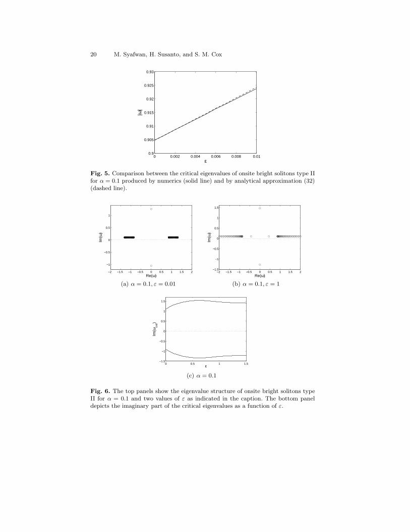
The (in)stability region of intersite bright solitons type I in the (ε, α)-plane is given by Fig. 10. In the figure, we also depict the two distinguish-able (solid and dashed) lines representing the two distinct critical eigenvalueswhose imaginary parts become zero. The star points on the lines correspondto those points in the right panels of Fig. 9. The boundary line which sepa-rates the stable and unstable regions in the figure is shown by the bold (solidand dashed) lines. The lower and upper dotted horizontal lines in the figurerepresent, respectively, α = αcp ≈ 0.4583 and α = αth ≈ 0.49659 which di-vide the region into three different descriptions of the eigenvalue structure.Interestingly, for αth < α, we can make an approximation for the numericallyobtained stability boundary (see the inset). This approximation is given byEq. (46) which is quite close to the numerics for small ε.
We notice in Fig. 10 that the solid line (not the rightmost) and dashedline also represent Hopf bifurcations, with one special point (the white-filledcircle) which does not meet the second condition for the occurrence of a (non-degenerate) Hopf bifurcation mentioned above. We will analyse the specialpoint in the next section. We see from the figure that the bold parts of theHopf lines coincide with the (in)stability boundary, while the nonbold ones

24 M. Syafwan, H. Susanto, and S. M. Cox
−2 −1 0 1 20
0.05
0.1
0.15
0.2
Re(ω)
Im(ω
)
(a) α = 0.1, ε = 0.08
−2 −1 0 1 2−0.05
0
0.05
0.1
0.15
0.2
Re(ω)
Im(ω
)
(b) α = 0.1, ε = 0.35
0 0.2 0.4 0.6−0.1
0
0.1
0.2
0.3
ε
Im(ω
crit)
(c) α = 0.1
−1.5 −1 −0.5 0 0.5 1 1.50
0.2
0.4
0.6
0.8
Re(ω)
Im(ω
)
(d) α = 0.465, ε = 0.02
−1.5 −1 −0.5 0 0.5 1 1.5−1
−0.5
0
0.5
1
1.5
2
Re(ω)
Im(ω
)
(e) α = 0.465, ε = 0.5
0 0.2 0.4 0.6
0
0.2
0.4
0.6
0.8
1
ε
Im(ω
crit)
(f) α = 0.465
−2 −1 0 1 20
0.2
0.4
0.6
0.8
1
Re(ω)
Im(ω
)
(g) α = 0.497, ε = 0.04
−2 −1 0 1 2−1
−0.5
0
0.5
1
1.5
2
Re(ω)
Im(ω
)
(h) α = 0.497, ε = 0.3
0 0.2 0.4 0.6
0
0.2
0.4
0.6
0.8
1
ε
Im(ω
crit)
(i) α = 0.497
Fig. 9. The first and second columns of panels show the structure of eigenvaluesof intersite bright solitons type I in the complex plane, for three values of α, eachof which uses two different values of ε, to depict the condition of stability (leftpanel) and instability (middle panel). The third column shows the imaginary partof the two distinct critical eigenvalues as functions of ε for the corresponding α. Thelocations of zero-crossings in these panels are indicated by the star markers.
exist in the unstable region. In addition, we also observe that the rightmostsolid line in Fig. 10 indicates the collection of branch points of pitchforkbifurcation experienced by the intersite type I, III, and IV; the bold part ofthis line also indicates the (in)stability boundary.
4.2.2 Intersite type II
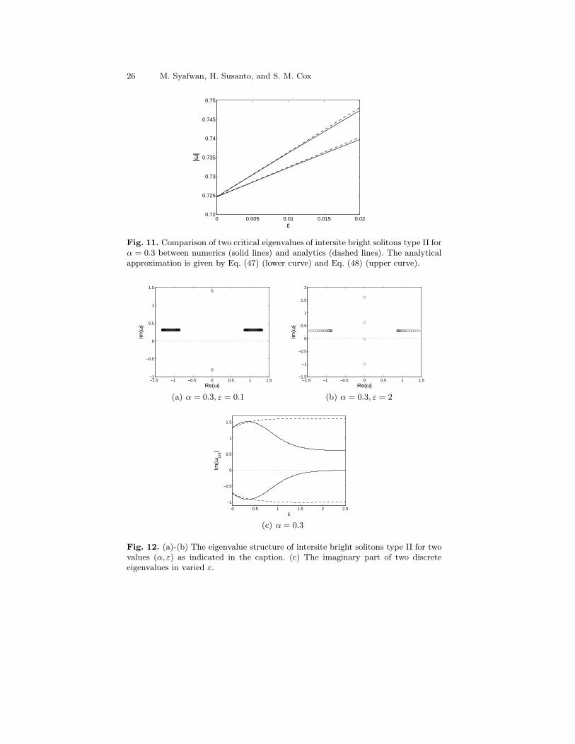
For intersite bright solitons type II, we present in Fig. 11 a comparison oftwo critical eigenvalues between the numerics and the analytical calculationgiven by Eqs. (47) and (48). We see from the figure that our approximationfor relatively small ε is quite close to the numerics. The snapshot of the eigen-value structure of this type of solution for two points (α, ε) and the path of
Solitons in a parametrically driven damped DNLS equation 25
ε
α
0 0.1 0.2 0.3 0.4 0.5 0.6 0.70
0.05
0.1
0.15
0.2
0.25
0.3
0.35
0.4
0.45
0.5
0 0.05 0.10.495
0.5
−1.4
−1.2
−1
−0.8
−0.6
−0.4
−0.2
0
0.2
0.4
stable
unstable
unstable unstable
Fig. 10. (Color online) As Fig. 4 but for intersite bright solitons type I. The bound-ary between stable and unstable regions is given by the bold (solid and dashed)lines. The dashed-dotted line in the inset is our analytical approximation given byEq. (46). The Hopf bifurcation lines are depicted by the solid (not the rightmost) anddashed lines. The white-filled circle indicates a degenerate Hopf point. The branchpoints of pitchfork bifurcation are shown by the rightmost solid lines.
the imaginary part of corresponding two discrete eigenvalues are depicted inFig. 12. We conclude that the intersite soliton type II is unstable even forlarge ε.
Moreover, the evaluation of the minimum value of Im(ω) of the intersitebright solitons type II in the (ε, α)-plane gives the (in)stability window (notshown here). It is shown that the soliton, except at the point α = γ = 0.5 andε = 0, is always unstable. This result agrees with our analytical prediction.
4.2.3 Intersite type III and IV
Now we examine the intersite bright soliton type III which, due to symmetry,has exactly the same eigenvalues as type IV. Shown in Fig. 13 is the analyticalapproximation for two critical eigenvalues given by Eqs. (49)-(50) or (51)-(52),which are compared with the corresponding numerical results. We concludethat the approximation is quite accurate for small ε and that the range ofaccuracy is wider for smaller value of α.
The structure of the eigenvalues of this type of solution and the curvesof the imaginary part of the corresponding two critical eigenvalues are givenby Fig. 14 for the three values of α used in Fig. 13. The figure reveals the
26 M. Syafwan, H. Susanto, and S. M. Cox
0 0.005 0.01 0.015 0.020.72
0.725
0.73
0.735
0.74
0.745
0.75
ε
|ω|
Fig. 11. Comparison of two critical eigenvalues of intersite bright solitons type II forα = 0.3 between numerics (solid lines) and analytics (dashed lines). The analyticalapproximation is given by Eq. (47) (lower curve) and Eq. (48) (upper curve).
−1.5 −1 −0.5 0 0.5 1 1.5−1
−0.5
0
0.5
1
1.5
Re(ω)
Im(ω
)
(a) α = 0.3, ε = 0.1
−1.5 −1 −0.5 0 0.5 1 1.5−1.5
−1
−0.5
0
0.5
1
1.5
2
Re(ω)
Im(ω
)
(b) α = 0.3, ε = 2
0 0.5 1 1.5 2 2.5
−1
−0.5
0
0.5
1
1.5
ε
Im(ω
crit)
(c) α = 0.3
Fig. 12. (a)-(b) The eigenvalue structure of intersite bright solitons type II for twovalues (α, ε) as indicated in the caption. (c) The imaginary part of two discreteeigenvalues in varied ε.

Solitons in a parametrically driven damped DNLS equation 27
condition of instability of solitons up to the limit points of ε at which theminimum imaginary part of the eigenvalues becomes zero; these conditions areindicated by the corresponding vertical lines in the third column. In fact, theselimit points indicate the branch points of pitchfork bifurcation experienced bythe intersite solitons type I, III, and IV (we will discuss this bifurcation inmore detail in the next section).
The first and second columns of Fig. 14 respectively present the conditionjust before and after a collision of one of the discrete eigenvalues which doesnot contribute to the instability of solitons. Interestingly, as shown in panel(c), such an eigenvalue also crosses the real axis at some critical ε as indicatedby the empty circle. The latter condition, in fact, indicates a Hopf bifurcation,which occurs when the soliton is already in unstable mode. This is differentfrom the previous discussions where the Hopf bifurcations also indicate thechange of stability of solitons.
0 0.005 0.01 0.015 0.02 0.025 0.030.8
0.9
1
1.1
1.2
1.3
1.4
1.5
1.6
1.7
1.8
ε
|ω|
(a) α = 0.1
0 0.002 0.004 0.006 0.008 0.010.4
0.5
0.6
0.7
0.8
0.9
1
ε
|ω|
(b) α = 0.465
0 0.2 0.4 0.6 0.8 1
x 10−3
0.2
0.25
0.3
0.35
0.4
ε
|ω|
(c) α = 0.497
Fig. 13. Comparisons between two critical eigenvalues of intersite bright solitons IIIand IV obtained numerically (solid lines) and analytically (dashed lines) for valuesof α as shown in the caption. In panels (a) and (b), the upper and lower dashedcurves correspond, respectively, to Eqs. (49) and (50), whereas in panel (c) theycorrespond to Eqs. (51) and (52).
28 M. Syafwan, H. Susanto, and S. M. Cox
Presented in Fig. 15 is the (in)stability window for intersite bright solitonstype III and IV which is defined as the area to the left of the solid line; thisline represents the set of the branch points of pitchfork bifurcation in the(ε, α)-plane. From the figure, we conclude that the intersite type III and IVare always unstable. The area to the right of the solid line belongs to theunstable region of intersite type I. One can check that this line is exactlythe same as the rightmost solid line in Fig. 10. In addition, the dashed lineappearing in Fig. 15 depicts the occurrence of Hopf bifurcations. However,there is one special point indicated by the white-filled circle, at which theε-derivative of the imaginary part of the corresponding critical eigenvalue iszero; this degenerate point will be discussed further in Sec. 5. The emptycircle lying on the Hopf line reconfirms the corresponding point in panel (c)of Fig. 14.
4.2.4 Saddle-node and pitchfork bifurcation of intersite bright
solitons
From both numerical and analytical results discussed above, we observed thatthe intersite type I and type II have the same profile and stability when ap-proaching α = γ. This fact indicates the appearance of a saddle-node bifur-cation undergone by the two solitons. Moreover, there also exists a pitchforkbifurcation experienced by the intersite type I, III, and IV.
One can check that the norm of the intersite type III and IV is exactlythe same for all parameter values so that this quantity can no longer be usedfor depicting a clear bifurcation diagram. Therefore, we now simply plot thevalue of |u0|2 for each solution, e.g., as a function of α and fixed ε = 0.1; thisis shown in Fig. 16 where the numerics (solid lines) is obtained by a pseudo-arc-length method. As seen in the figure, the intersite type I, III, and IV meetat a (pitchfork) branch point (BP) α ≈ 0.49. At this point, the stability ofthe intersite type I is switched. Furthermore, the intersite type I and II alsoexperience a saddle-node bifurcation where they merge at a limit point (LP)α = γ = 0.5. Just before this point, the intersite type I possesses one unstableeigenvalue, while the type II has two unstable eigenvalues. The two criticaleigenvalues for the intersite type I and II then coincide at LP. We confirmthat our analytical approximation for the value of |u0|2 is relatively close tothe corresponding numerical counterpart.
Next, let us plot the value of |u0|2 for each soliton by fixing α = 0.1 andvarying ε (presented in Fig. 17). The pitchfork bifurcation experienced by theintersite type I (solid line), type III (upper dashed line), and type IV (lowerdashed line) is clearly shown in the figure. The three solitons meet togetherat a branch point BP. We also depict in the figure the points at which Hopfbifurcations emerge (labelled by indexed H). For the shake of completeness,we also plot the relevant curve for the intersite type II (dotted line).

Solitons in a parametrically driven damped DNLS equation 29
−2 −1 0 1 2−1.5
−1
−0.5
0
0.5
1
1.5
Re(ω)
Im(ω
)
(a) α = 0.1, ε = 0.1
−2 −1 0 1 2
−0.5
0
0.5
1
Re(ω)
Im(ω
)
(b) α = 0.1, ε = 0.5
0 0.2 0.4 0.6
−1
−0.5
0
0.5
1
ε
Im(ω
crit)
(c) α = 0.1
−1 −0.5 0 0.5 1−0.5
0
0.5
1
1.5
Re(ω)
Im(ω
)
(d) α = 0.465, ε = 0.01
−1 −0.5 0 0.5 1−0.5
0
0.5
1
1.5
Re(ω)
Im(ω
)
(e) α = 0.465, ε = 0.15
0 0.05 0.1 0.15 0.2−0.5
0
0.5
1
ε
Im(ω
crit)
(f) α = 0.465
−1 −0.5 0 0.5 1−0.2
0
0.2
0.4
0.6
0.8
1
1.2
Re(ω)
Im(ω
)
(g) α = 0.497, ε = 0.005
−1 −0.5 0 0.5 1−0.2
0
0.2
0.4
0.6
0.8
1
1.2
Re(ω)
Im(ω
)
(h) α = 0.497, ε = 0.04
0 0.02 0.04 0.06−0.2
0
0.2
0.4
0.6
0.8
1
ε
Im(ω
crit)
(i) α = 0.497
Fig. 14. (First and second columns) The structure of eigenvalues of intersite brightsolitons type III and IV for parameter values (α, ε) as indicated in the caption.(Third column) The imaginary part of two critical eigenvalues obtained by varyingε. The vertical lines indicate the limit points of ε up to which the soliton exists, i.e.,when the minimum imaginary part of the eigenvalues becomes zero.
5 Nature of Hopf bifurcations and continuation of limit
cycles
If there is only one pair of non-zero real eigenvalues and the other eigenval-ues have strictly positive imaginary parts, a Hopf bifurcation also indicatesthe change of stability of the steady state solution. In this case, the periodicsolutions bifurcating from the Hopf point coexist with either the stable or un-stable mode of the steady state solution. If the periodic solutions coexist withthe unstable steady state solution, they are stable and the Hopf bifurcation iscalled supercritical. On the other hand, if the periodic solutions coexist withthe stable steady state solution, they are unstable and the Hopf bifurcationis called subcritical.

30 M. Syafwan, H. Susanto, and S. M. Cox
ε
α
0 0.1 0.2 0.3 0.4 0.5 0.6 0.70
0.05
0.1
0.15
0.2
0.25
0.3
0.35
0.4
0.45
0.5
−1.4
−1.2
−1
−0.8
−0.6
−0.4
−0.2
0
Intersite type II(unstable)
Intersite type III and IV(unstable)
Fig. 15. The (in)stability region of intersite bright solitons type III and IV in(ε, α)-space. The solid line indicates the branch-point line of pitchfork bifurcation.The dashed line represents the occurrence of Hopf bifurcations (with one degeneratepoint at the white-filled circle), which arises from one of the critical eigenvalueswhich does not contribute to the instability of solitons. The empty circle lying onthe dashed line corresponds to that point depicted in panel (c) of Fig. 14.
To numerically calculate the first Lyapunov coefficient for a Hopf pointand perform a continuation of the bifurcating limit cycle, we use the numericalcontinuation package Matcont. Due to the limitations of Matcont, we evaluatethe soliton using 21 sites. In fact, this setting does not affect significantly thesoliton behavior compared to that used in the previous section.
In this section, we examine the nature of Hopf points and the stability ofcycle continuations in onsite type I, intersite type I, and intersite type III-IV.
5.1 Onsite type I
For this type of solution, in particular at α = 0.1, we have one Hopf point,which occurs at εc ≈ 0.3077 (see again panel (c) in Fig. 3). From Matcont,we obtain l1(εc ≈ 0.3077) > 0 which indicates that the Hopf point εc is sub-critical and hence the limit cycle bifurcating from this point is unstable. Acontinuation of the corresponding limit cycle is given in Fig. 18(a). As theHopf point in this case also indicates the change of stability of the station-ary soliton, one can confirm that the bifurcating periodic solitons are stablebecause they coexist with the stable onsite type I; this agrees with the com-puted first Lyapunov coefficient above. Interestingly, the continuation of the

Solitons in a parametrically driven damped DNLS equation 31
0 0.1 0.2 0.3 0.4 0.5 0.6
0.4
0.6
0.8
1
1.2
1.4
1.6
1.8
2
α
|u0|2
−5 0 5
00.5
11.5
α=0.1
−5 0 5−1
0
1
α=0.1
−5 0 5−1
−0.5
0
α=0.1
−5 0 5−1
0
1
α = 0.1
−5 0 5−1
0
1
α = 0.5
−5 0 5−1
0
1
α ≈ 0.49
intersite type IV(unstable)
intersite type II (unstable)
intersite type III(unstable)
intersite type I (stable)
BP
LP
intersite type I (unstable)
Fig. 16. Saddle-node and pitchfork bifurcations of intersite bright solitons by vary-ing α and fixing ε = 0.1. The curves depict the value of |u0|
2 of each solutionsobtained numerically (solid lines) and analytically (dashed lines). The profiles ofthe corresponding solutions at some values of α are shown in the relevant insets.The intersite type I, III, and IV merge at a branch point (BP) α ≈ 0.49 and theintersite type I and II meet at a limit point (LP) α = γ = 0.5.
limit cycle also experiences saddle-node and torus bifurcations, as indicatedby the points labelled LPC (limit point cycle) and NS (Neimark-Sacker), re-spectively. The profile of a representative periodic soliton over one period isshown in Fig. 18(b), from which we clearly see the typical oscillation in thesoliton amplitude.
From the previous discussion we have mentioned that there is one degen-erate point for Hopf bifurcations in onsite type I, which is indicated by thewhite-filled circle in Fig. 4. In Fig. 19, we depict numerical continuations of pe-riodic orbits of two Hopf bifurcations near the degenerate point. We obtainedthat the limit cycle branches bifurcating from the Hopf points are connectedand form a closed loop. This informs us that as α approaches the critical valuefor a degenerate Hopf point, the “radius” of the loop tends to zero. Hence,one may conclude that at the double-Hopf point, there is no bifurcation ofperiodic orbits.
5.2 Intersite type I
In particular for α = 0.1, there are three Hopf points detected for the inter-site type I (see again Fig. 17). For point H1 (ε ≈ 0.2782), Matcont gives anegative value for the first Lyapunov coefficient, which means that the bifur-cating periodic soliton is stable or H1 is supercritical. The corresponding cycle

32 M. Syafwan, H. Susanto, and S. M. Cox
0 0.1 0.2 0.3 0.4 0.5 0.6 0.70.4
0.6
0.8
1
1.2
1.4
1.6
1.8
2
2.2
ε
|u0|2
BPH
2
H3
H1
H4
H5
Fig. 17. A pitchfork bifurcation of intersite bright solitons for fixed α = 0.1 andvaried ε. The curves represent the numerical value of |u0|
2 for the correspondingsolutions as a function of ε. The intersite type I (dashed line), type III (upperdashed line), and type IV (lower dashed line) merge at a branch point (BP). Theoccurrence of Hopf bifurcation (Hi) is detected in intersite type I, III, and IV. Thedotted line corresponds to the intersite type II.
0.25 0.26 0.27 0.28 0.29 0.3 0.31 0.321.1
1.2
1.3
1.4
1.5
1.6
1.7
1.8
1.9
ε
max
(||u
n||), m
in(|
|un||)
H
LPCNS
(a)
−10−5
05
10
0
1.7160
3.43190
0.5
1
1.5
nt
|un|
(b)
Fig. 18. (a) The continuation of the limit cycle from a Hopf point H for an onsitesoliton type I with α = 0.1. The first Lyapunov coefficient for H calculated byMatcont is positive, i.e. H is subcritical. The bold solid line represents the normof the stationary soliton while the solid and dashed lines indicate, respectively, themaximum and minimum of the norm of the bifurcating periodic solitons. (b) Theprofile of an unstable periodic soliton (as H is subscritical) over one period (T ≈3.4319) corresponding to the black-filled circle in panel (a).

Solitons in a parametrically driven damped DNLS equation 33
1.45 1.455 1.46 1.465 1.47
2.054
2.056
2.058
2.06
2.062
2.064
ε
max
(||u
n||), m
in(|
|un||)
Fig. 19. As Fig. 18(a) but for α = 0.492642. Two Hopf points (stars) in the neigh-bourhood of the degenerate point (the while-filled circle in Fig. 4) are shown to beconnected by a branch of limit cycles.
continuation is presented in Fig. 20(a). As shown in the figure, the limit cy-cle bifurcating from H1 coexist with the unstable mode of the (steady-state)intersite type I which confirms the supercritical H1. This is valid becausethe Hopf bifurcation in this case also indicates the change of stability of thesoliton. We also see from the figure that the cycle continuation contains NS,LPC, and BPC (branch point cycle) points which indicate the occurrenceof, respectively, torus, saddle-node, and pitchfork bifurcations for limit cycle.The branches of the cycle continuation from the BPC point are shown in thefigure. A representative periodic soliton (in one period) which occurs at onerepresentative point along the cycle continuation is depicted in Fig. 20(b),which shows the oscillation between the two excited sites.
Next, for H2 (ε ≈ 0.3871) and H3 (ε ≈ 0.4934), the first Lyapunov coeffi-cients given by Matcont are negative and positive valued, respectively. Thus,H2 is supercritical while H3 is subcritical, which implies that the limit cyclebifurcating from H2 and H3 are stable and unstable, respectively. The contin-uations of the corresponding limit cycles are shown in Fig. 21(a). From thefigure, we see that the limit cycles bifurcating from H2 and H3 respectivelycoexist with the unstable and stable stationary intersite soliton type I. Thisfact is consistent with the nature of H2 and H3 as given by Matcont. In ad-dition, as shown in the figure, a period-doubling (PD) bifurcation also occursin the cycle continuation coming from H3. This bifurcation seems to coincidewith the turning point of cycle (LPC) which appears in the cycle continua-tion starting from H2. The profile of one-period periodic solitons at the tworepresentative points near H2 and H3 are presented in Figs. 21(b) and 21(c),respectively. We cannot see clearly the typical oscillation of the periodic soli-

34 M. Syafwan, H. Susanto, and S. M. Cox
0.25 0.26 0.27 0.28 0.29
1
1.5
2
2.5
3
ε
max
(|u 0|2 ),
min
(|u 0|2 )
LPCBPCNS
LPCBPCNS
H1
(a)
−10−5
05
10
0
2.7633
5.52650
0.5
1
1.5
nt
|un|
(b)
0.27 0.271 0.272 0.273 0.274 0.275 0.276
2.46
2.48
2.5
2.52
2.54
2.56
2.58
2.6
2.62
2.64
ε
max
(|u 0|2 ),
min
(|u 0|2 )
LPCBPCNS
(c)
0.272 0.274 0.276 0.278 0.28
1.05
1.1
1.15
1.2
1.25
1.3
1.35
ε
max
(|u 0|2 ),
min
(|u 0|2 )
LPCBPCNS
(d)
Fig. 20. (a) The cycle continuation from Hopf point H1 for intersite bright solitontype I with α = 0.1. In this case, H1 is supercritical. The bold solid line indicates thevalue of |u0|
2 for the stationary soliton, which is the same as that shown in Fig. 17.The solid and dashed lines represent, respectively, the maximum and minimum valueof |u0|
2 for the bifurcating periodic solitons, which also experience a pitchfork cyclebifurcation. The branches of the cycle are depicted by the dash-dotted (maximum|u0|
2) and dotted (minimum |u0|2) lines. (b) The profile of a stable periodic soliton
(as H1 is supercritical) over one period (T ≈ 5.5265) corresponding to the star pointin panel (a). (c,d) Enlargements of, respectively, the upper and the lower rectanglesin panel (a).
.
ton in Fig. 21(b) as it occurs very near to H2. By contrast, the oscillation inthe soliton amplitude is clearly visible in Fig. 21(c).
Similarly to the onsite type I, we also noticed the presence of a double-Hopf bifurcation in the intersite type I, i.e., the white-filled circle in Fig. 10.To investigate the point, we evaluate several Hopf points nearby the bifur-cation point and perform numerical continuations for limit cycles, which arepresented in Fig. 22. Unlike the case in the onsite type I, here the (non-degenerate) Hopf points are not connected to each other by a closed loop of abranch of limit cycles. As we observe this scenario at any Hopf point that is

Solitons in a parametrically driven damped DNLS equation 35
0.38 0.4 0.42 0.44 0.46 0.48 0.5
1.4
1.6
1.8
2
2.2
2.4
2.6
LPC
LPC
ε
max
(|u 0|2 ),
min
(|u 0|2 )
PD
PD
0.387 0.3872
1.78
1.8
1.82
1.84LPCPDNS
H3
H2
H2
(a)
−10−5
05
10
0
3.354
6.7080
0.5
1
1.5
nt
|un|
(b)
−10−5
05
10
0
1.7493
3.49850
0.5
1
1.5
nt
|un|
(c)
Fig. 21. (a) As Fig. 20(a) but for H2 and H3, where the inset gives the zoom-in forthe corresponding region showing that H2 and H3 are supercritical and subcritical,respectively. The bold solid line is the same as that shown in Fig. 17, i.e., representingthe value of |u0|
2 for the stationary intersite soliton. The solid (dashed) and dash-dotted (dotted) lines shows the maximum (minimum) value of |u0|
2 for the periodicsoliton which bifurcates from, respectively, H2 and H3. (b,c) The profile of periodicsolitons over one period T ≈ 6.708 and T ≈ 3.4985 which corresponds, respectively,to the star and the black-filled circle in panel (a). From the nature of H2 and H3,periodic solitons in (b) and (c) are stable and unstable, respectively.
36 M. Syafwan, H. Susanto, and S. M. Cox
arbitrarily close (up to a numerical accuracy) to the degenerate (codimension2) bifurcation, it indicates that at the double-Hopf point, there is a bifurcationof at least two branches of periodic solutions.
0.33 0.34 0.35 0.36 0.371.5
1.6
1.7
1.8
1.9
2
2.1
2.2
ε
max
(|u 0|2 ),
min
(|u 0|2 )
LPC
LPC
LPC
LPC
LPC
LPC
Fig. 22. As Fig. 21(a) but for α = 0.108 (triangles) and α = 0.11082 (stars) in theproximity of the while-filled circle in Fig. 15.
5.3 Intersite type III and IV
As intersite bright soliton type III and IV possess the same eigenvalue struc-tures, the nature of the corresponding Hopf bifurcation and the stability ofthe continuation of each limit cycle will be the same as well. Therefore it issufficient to devote our discussion to intersite type III only.
As shown in Fig. 17, there is one Hopf point, namely H4, for the intersitetype III at α = 0.1. In this type of solution, the Hopf bifurcation occurs whileother eigenvalues already give rise to instability; this is different from thetype of Hopf bifurcation discussed previously. Therefore we cannot performthe analysis as before in determining the stability of the bifurcating periodicsoliton. In fact, according to calculation given by Matcont, the first Lyapunovcoefficient for H4 is positive (subcritical), which means that the bifurcatingperiodic soliton is unstable.
Fig. 23(a) shows the continuation of the corresponding limit cycle fromH4. A representative one-period periodic soliton at ε near H4 (indicated bythe black-filled circle) is shown in Fig. 23(b), from which we can see clearlythe oscillation in the amplitude of soliton.
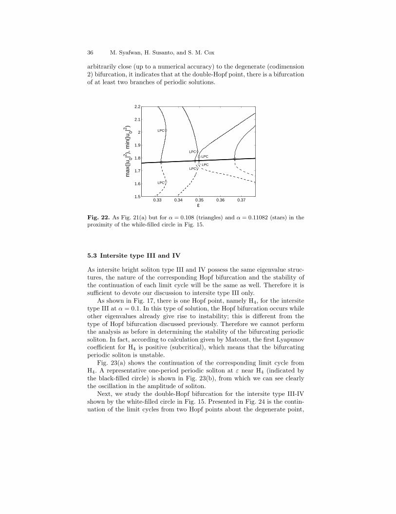
Next, we study the double-Hopf bifurcation for the intersite type III-IVshown by the white-filled circle in Fig. 15. Presented in Fig. 24 is the contin-uation of the limit cycles from two Hopf points about the degenerate point,
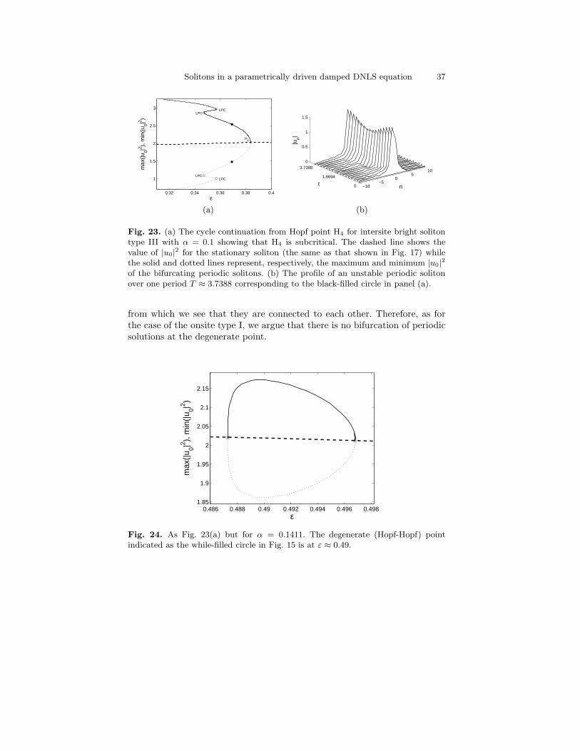
Solitons in a parametrically driven damped DNLS equation 37
0.32 0.34 0.36 0.38 0.4
1
1.5
2
2.5
3
H4
ε
max
(|u 0|2 ),
min
(|u 0|2 )
LPC
LPC
LPC
LPC
(a)
−10−5
05
10
0
1.8694
3.73880
0.5
1
1.5
nt
|un|
(b)
Fig. 23. (a) The cycle continuation from Hopf point H4 for intersite bright solitontype III with α = 0.1 showing that H4 is subcritical. The dashed line shows thevalue of |u0|
2 for the stationary soliton (the same as that shown in Fig. 17) whilethe solid and dotted lines represent, respectively, the maximum and minimum |u0|
2
of the bifurcating periodic solitons. (b) The profile of an unstable periodic solitonover one period T ≈ 3.7388 corresponding to the black-filled circle in panel (a).
from which we see that they are connected to each other. Therefore, as forthe case of the onsite type I, we argue that there is no bifurcation of periodicsolutions at the degenerate point.
0.486 0.488 0.49 0.492 0.494 0.496 0.4981.85
1.9
1.95
2
2.05
2.1
2.15
ε
max
(|u 0|2 ),
min
(|u 0|2 )
Fig. 24. As Fig. 23(a) but for α = 0.1411. The degenerate (Hopf-Hopf) pointindicated as the while-filled circle in Fig. 15 is at ε ≈ 0.49.

38 M. Syafwan, H. Susanto, and S. M. Cox
6 Conclusion
In this paper, we have considered a parametrically driven damped discretenonlinear Schrodinger (PDDNLS) equation. The existence and stability offundamental discrete bright solitons have been examined analytically througha perturbation theory for small ε and then corroborated by numerical calcu-lations. We showed that there are two types of onsite discrete soliton, namelyonsite type I and II. For onsite type I, we found an interval in α for which thesoliton is stable for any coupling constant, i.e., a damping can re-stabilize adriven onsite soliton. Contrastingly, the onsite type II was found to be alwaysunstable for all ε. These two solitons experience a saddle-node bifurcationwith the limit point α = γ for any ε.
We also showed that there are four types of intersite discrete soliton, calledintersite type I, II, III, and IV. In fact, intersite type III and IV are essentiallyconsidered as one solution due to its symmetry. We obtained that intersite typeI in the region of instability in the non-dissipative case can be stabilized bydamping while intersite type II and III-IV are always unstable. A saddle-nodebifurcation, as for the onsite soliton, was found to be undergone by intersitetype I and II. Moreover, we also obtained that intersite type I, III, and IVexperience a pitchfork bifurcation. The branch points of such a bifurcation inthe (ε, α)-plane have been calculated numerically.
More interestingly, we observed that Hopf bifurcation also occurs in onsitetype I, intersite type I, and intersite type III-IV, which confirms the existenceof the corresponding periodic solitons (limit cycles) in the PDDNLS equation.The continuation of the limit cycles as well as the stability of the periodicsolitons have been demonstrated numerically using the numerical continuationsoftware Matcont. In particular, subcritical Hopf bifurcations for onsite typeI and intersite type III-IV were observed. Moreover, we obtained three Hopfbifurcations for intersite type I. It was shown that two of these points generatestable periodic solitons, i.e. the bifurcations are supercritical.
Note that similar studies for the continuum limit of Eq. (1) have been putforward in, e.g., Refs. [24, 25, 26]. Hopf bifurcations and the correspondingperiodic solitons were reported and discussed therein. The connection betweenthe results presented in this work, which correspond to weakly coupled lattices,and those of [24, 25, 26] are proposed for future study.
Acknowledgments
The authors thank to Hill Meijer for fruitful discussions and guidance onMatcont. MS acknowledges financial support from the Ministry of NationalEducation of the Republic of Indonesia.

Solitons in a parametrically driven damped DNLS equation 39
References
1. P. G. Kevrekidis (Editor), Discrete Nonlinear Schrodinger Equation: Mathe-
matical Analysis, Numerical Computations and Physical Perspectives (Springer:New York, 2009).
2. P. G. Kevrekidis, K. O. Rasmussen and A. R. Bishop, The discrete nonlinear
Schrodinger equation: A survey of recent results, Int. J. Mod. Phys. B 15, 2833(2001).
3. D. Hennig and G. Tsironis, Wave transmission in nonlinear lattices, Phys. Rep.307, 333 (1999).
4. G. L. Alfimov, V. A. Brazhnyi and V. V. Konotop, On classification of intrinsic
localized modes for the discrete nonlinear Schrodinger equation, Physica D 194,127 (2004).
5. D. E. Pelinovsky, P. G. Kevrekidis and D. J. Frantzeskakis, Stability of discrete
solitons in nonlinear Schrodinger lattices, Physica D 212, 1 (2005).6. E. P. Fitrakis, P. G. Kevrekidis, H. Susanto and D. J. Frantzeskakis, Dark
solitons in discrete lattices: Saturable versus cubic nonlinearities, Phys. Rev. E75, 066608 (2007).
7. M. Johansson and Yu. S. Kivshar, Discreteness-induced oscillatory instabilities
of dark solitons, Phys. Rev. Lett. 82, 85 (1999).8. Yu. S. Kivshar, W. Krolikowski and O. A. Chubykalo, Dark solitons in discrete
lattices, Phys. Rev. E 50, 5020 (1994).9. H. Susanto and M. Johansson, Discrete dark solitons with multiple holes, Phys.
Rev. E 72, 016605 (2005).10. D. E. Pelinovsky and P. G. Kevrekidis, Stability of discrete dark solitons in
nonlinear Schrodinger lattices, J. Phys. A. 41, 185206 (2008).11. H. Susanto, Q. E. Hoq and P. G. Kevrekidis, Stability of discrete solitons in the
presence of parametric driving, Phys. Rev. E 74, 067601 (2006).12. M. Syafwan, H. Susanto, and S. M. Cox, Discrete solitons in electromechanical
resonators, Phys. Rev. E 81, 026207 (2010).13. N. V. Alexeeva, I. V. Barashenkov and G. P. Tsironis, Impurity-induced sta-
bilization of solitons in arrays of parametrically driven nonlinear oscillators,Phys. Rev. Lett. 84, 3053 (2000).
14. I. V. Barashenkov, N. V. Alexeeva and E. V. Zemlyanaya, Two- and three-
dimensional oscillons in nonlinear faraday resonance, Phys. Rev. Lett. 89,104101 (2002).
15. N. V. Alexeeva, Stabilization mechanism for two-dimensional solitons in non-
linear parametric resonance, Theor. Math. Phys. 144, 1075 (2005).16. I. V. Barashenkov, E. V. Zemlyanaya and M. Bar, Traveling solitons in the
parametrically driven nonlinear Schrodinger equation, Phys. Rev. E 64, 016603(2001).
17. I. V. Barashenkov, S. R. Woodford and E. V. Zemlyanaya, Parametrically
driven dark solitons, Phys. Rev. Lett. 90, 054103 (2003).18. I. V. Barashenkov, S. Cross and B. A. Malomed, Multistable pulselike solutions
in a parametrically driven Ginzburg-Landau equation, Phys. Rev. E 68, 056605(2003).
19. I. V. Barashenkov and S. R. Woodford, Complexes of stationary domain walls
in the resonantly forced Ginzburg-Landau equation, Phys. Rev. E 71, 026613(2005).

40 M. Syafwan, H. Susanto, and S. M. Cox
20. I. V. Barashenkov, S. R. Woodford and E. V. Zemlyanaya, Interactions of
parametrically driven dark solitons. I. Neel-Neel and Bloch-Bloch interactions,Phys. Rev. E 75, 026604 (2007).
21. I. V. Barashenkov and S. R. Woodford, Interactions of parametrically driven
dark solitons. II. Neel-Bloch interactions, Phys. Rev. E 75, 026605 (2007).22. D. Hennig, Periodic, quasiperiodic, and chaotic localized solutions of a driven,
damped nonlinear lattice, Phys. Rev. E 59, 1637 (1999).23. M. Kollmann, H. W. Capel and T. Bountis, Breathers and multibreathers in a
periodically driven damped discrete nonlinear Schrodinger equation, Phys. Rev.E 60, 1195 (1999).
24. M. Bondila, I. V. Barashenkov and M. M. Bogdan, Topography of attractors of
the parametrically driven nonlinear Schrodinger equation, Physica D 87, 314(1995).
25. I. V. Barashenkov, E. V. Zemlyanaya and T. C. van Heerden, Time-periodic
solitons in a damped-driven nonlinear Schrodinger equation, Phys. Rev. E 83,056609 (2011).
26. I. V. Barashenkov and E. V. Zemlyanaya, Soliton complexity in the damped-
driven nonlinear Schrodinger equation: Stationary to periodic to quasiperiodic
complexes, Phys. Rev. E 83, 056610 (2011).27. R. S. MacKay and S. Aubry, Proof of existence of breathers for time-reversible
or Hamiltonian networks of weakly coupled oscillators, Nonlinearity 7, 1623(1994).
28. P. G. Kevrekidis, A. R. Bishop, and K. Ø. Rasmussen, Twisted localized modes,Phys. Rev. E 63, 036603 (2001).
29. Y. A. Kuznetsov: Elements of Applied Bifurcation Theory (Applied Mathemat-ical Sciences Vol. 112), 2nd edn, (Springer-Verlag, New York 1998)