Soliton solutions of nonlinear Dirac equationsK. Takahashi Citation: Journal of Mathematical Physics 20, 1232 (1979); doi: 10.1063/1.524176 View online: http://dx.doi.org/10.1063/1.524176 View Table of Contents: http://scitation.aip.org/content/aip/journal/jmp/20/6?ver=pdfcov Published by the AIP Publishing Articles you may be interested in Ground state solutions for nonperiodic Dirac equation with superquadratic nonlinearity J. Math. Phys. 54, 101502 (2013); 10.1063/1.4824132 Asymptotic stability of small gap solitons in nonlinear Dirac equations J. Math. Phys. 53, 073705 (2012); 10.1063/1.4731477 On the integrability of nonlinear Dirac equations J. Math. Phys. 25, 2331 (1984); 10.1063/1.526404 Similarity solutions of nonlinear Dirac equations and conserved currents J. Math. Phys. 23, 145 (1982); 10.1063/1.525202 Solitons and rational solutions of nonlinear evolution equations J. Math. Phys. 19, 2180 (1978); 10.1063/1.523550

This article is copyrighted as indicated in the article. Reuse of AIP content is subject to the terms at: http://scitation.aip.org/termsconditions. Downloaded to IP:

128.59.226.54 On: Tue, 09 Dec 2014 06:14:14

Soliton solutions of nonlinear Dirac equations K. Takahashi

Department of Physics, Tohoku University, Sendai 980, Japan (Received 26 October 1978)

Dirac equations with fourth order self-couplings are investigated in one time and three space dimensions. Both stringlike and ball-like soliton solutions carrying nontopological quantum numbers are shown to exist, depending on the symmetries taken into account. The energies (per unit length) of stringlike solutions turn out to be always smaller than those of plane wave solutions. For ball-like solutions, it is shown that the region of values of the non topological quantum numbers exists in which the total energies of solitons are smaller than those of plane waves.

1. INTRODUCTION

Soliton solutions of nonlinear field equations have been studied in detail in the last few years. 1 They have finite spa­tial extensions and finite energies and are regarded as candi­dates for models of elementary particles. These soliton solu­tions are classified into two categories: topological and nontopological solitons.z,} The stability of topological soli­tons is expected to some degree from their topological quan­tum numbers, while U(1) charges play an important role for the stability of non topological solitons. We investigate non­topological solitons in this article.

Models are given by Lagrangians (1.1) or (3.1), which describe systems of self-interacting Dirac spinors. The space-time is four-dimensional. Analogous models in one time and one space dimension have already been studied' and exact solutions are known. Also, in four-dimensional space-time, exact solutions can be obtained by introducing a peculiar interaction. s In the present case, however, we shall have recourse to computer calculations at the final step of the investigation.

We start our discussions by considering plane wave so­lutions for the model

5e 1 = ¢(io - m)¢ + gZ (¢¢)2, 2

(1.1)

where ¢ is a four component Dirac spinoe Throughout this paper we are concerned with the case in which the force is attractive (i.e., gZ > 0) when ¢ is regarded as a quantized Fer­mi field. The equation of motion is

(iiJ - m)¢ + gZ(ij,¢)¢ = o. The energy and charge density are given by

cyp .7.( . i a ).,. g2 (.7..,,)2 eN ! = 'I' - ly-. + m 'I' - - '1''1' ,

aX' 2 p = ¢t¢.

The lowest energy plane wave of the form

(1.2)

(1.3)

(1.4)

(1.5)

where u and v are constant two component spinors, satisfies

(1.2) if

t m-{j) u u = --z-, V = O.

g (1.6)

Here we have confined the whole system into a large cube of volume 11 and imposed the periodic boundary condition. The total energy and the total charge are given by

m -(j) Q=pfl=--fl.

g2

(1.7)

(1.8)

Fixing Q and taking the limit 11---+ 00 , we obtain the expected result

E=Qm. (1.9)

Thus, for a given Q, the energy of a stable soliton must be smaller than Qm.

In Sec. 2, we shall see that there exist stringlike solu­tions for the U(1) invariant model (1.1). Given a charge Q per unit length along the string, the energy per unit length is always smaller than Qm. In Sec. 3, ball-like solutions with finite spatial extensions in the three-dimensional space are found. The associated group is SO(3). Computer calcula­tions in Sec. 4 show that there is a region of Q in which the energies of solitons are smaller than Qm.

2. STRINGLIKE SOLUTIONS A. Equation of motion

In this section we solve Eq. (1.2) and seek cylindrically symmetric solutions, whose axis lies along the Xl direction, under the ansatz

¢(p,t) = e - ivmt + in~(i~ !/J,(p) + ¢2(p»).

2 2 i= - I y'x i = I y'x i, (2.1)

i= 1 i= 1

where v is a real number whose sign we set to be positive. cp is the azimuthal angle around the Xl axis. In order that ¢ is single-valued, n must be an integer. p is the distance from the Xl axis:p = (xi + XDIIZ. ¢, and ¢2 are real functions ofp only.

1232 J. Math. Phys. 20(6). June 1979 0022-2488179/061232-07$01.00 CD 1979 American Institute of PhYSics 1232

This article is copyrighted as indicated in the article. Reuse of AIP content is subject to the terms at: http://scitation.aip.org/termsconditions. Downloaded to IP:

128.59.226.54 On: Tue, 09 Dec 2014 06:14:14

For r matrices, we adopt the notation of Bjork en and Orell.6

One may recognize that the appearance of the phase factor expin¢ in (2.5) is similar to the situation for the Higgs field in the Ginzburg-Landau type equation studied by Nielsen and Olesen. 2 However, we are interested in solutions which van­ish at infinity so that no topological quantum number will emerge.

The substitution of (2.1) in Eq. (1.2) gives a complex coupled equation in 1/11 and 1/12' However, if 1/11 and 1/12 are eigenfunctions ofY' with the same eigenvalue, - P, Eq. (1.2) reduces to a simpler form owing to the equalities ¢ktl/11 = O. In fact, requiring the coefficients of expi( - vmt + n¢ ) and expi( - vm t + n¢ );1 in Eq. (1.2) to vanish independen tly, we obtain a set of equations

~1/11 + ~1 + n~,)r/JI - m(l + VP)1/12 + g2(¢r/J)r/J2 = 0,

dp P (2.2)

~r/J2 - !!..~;tP2 - m(l - VP)tPI + g2(¢tP)tPI = O. (2.3) dp p

Here.I, = (i/2)[y1 ,r2] and ¢tP = - ¢ltPI + ¢2r/J2'

The simultaneous presence of the second tenns of (2.2) and (2.3) will, in general, hinder us from finding a solution nonsingular atp = 0 and nondivergent atp = 00. Therefore, we have to impose as a condition either n.I,tPI = - tPI or n = O. Since we see that the interchange of conditions ! n.I, = - I,P l+--+! n = 0, - P I simply means the inter­change of tPI and tP2, it is sufficient to treat the case n.IJ = - 1 for both P = + 1 and P = - 1. For definite­ness, we set n = + 1. This means .I, = - 1 (note that tPI and tP2 must have the same eigenvalue of .IJ) and the fonns of tPk are

tPI(P) = [ ~ ],

f(p)

for P = + 1, (2.4)

¢,(p) ~ r~)l for P = - 1, (2.5)

B. Special limit

First, consider the case P = + I. Equations (2.2) and (2.3) can be rewritten in terms of/and has

~/ - m(l + v)h + g2(f2 - h 2)h = 0, (2.6) dp

~h + ~h - m(1 - v)f + g2(f2 - h 2) = O. (2.7) dp P

Since it is not manifest whether or not these equations have nontrivial solutions, we investigate this point by adopting the tactics used in Ref. 3, i.e., we assume that solutions of Eqs. (2.6) and (2.7), if any, approach the plane wave solution as S = (m( 1 - V»II2-<J •. The following expansion in S turns out to be of much use for our purpose:

/= Sa(r) + ... ,

1233 J. Math. Phys., Vol. 20, No.6, June 1979

(2.8)

where r=Y 2m Sp. Substituting (2.8) into (2.6), one finds

da = (3, (2.9) d1'

and from (2.7)

d'{J 1 - + -(3 - a + g2a J = O. d1' l'

(2.10)

From (2.9) and (2.10), one obtains a differential equation for a,

d 2a 1 da 2 J 0 --+---a+ga = . d1'2 l' dr

(2.11)

As mentioned in Ref. 3, Eq. (2.11) can be looked upon as describing the motion of a point particle in a potential

1 2 v= _--a2 +~4, 2 4

(2.12)

and under the action of a frictional force

1 da Fj = ---.

l' dr

Soliton solution must satisfy the boundary conditions

and

da = 0, at l' = 0 d1'

a-<J, when 1'-00.

(2.13)

(2.14)

Note that (2.13) together with (2.9) requires (3 to vanish at l' = 0 and assures the regularity of tP given by (2.1). (2.14) may be necessary for the sake of Lorentz in variance of the vacuum.

An infinite number of solutions are known to exist, which are specified by the number of radial nodes. The solu­tion with the lowest energy (per unit length) has no radial nodes. The total energy per unit length of the soliton is the integration of the Hamiltonian density:

(2.15) where Q is the total charge per unit length,

(2.16)

The second term on the right-hand side ofEq. (2.15) vanish­es identically. This can be seen in the following way. First, note that Eq. (2.10) is just the condition that the quantity A defined by

A = rdr - - + --a2 - !La-i "'" [ 1 (da)2 1 2]

o 2 dr 2 4 (2.17)

K. Takahashi 1233

This article is copyrighted as indicated in the article. Reuse of AIP content is subject to the terms at: http://scitation.aip.org/termsconditions. Downloaded to IP:

128.59.226.54 On: Tue, 09 Dec 2014 06:14:14

should be stationary under small variations of a,

c5A = 0. c5a

(2.18)

Now, we scale a: a(r)-aPa(ar). Then (2.17) becomes

A (a) = a2PK + a2p ~ 2Ll - a4p ~ 2L,. (2.19)

K, L l , and L, are defined by

K=- rdr-, 1 l'" (da)2 2 0 dr

Ll = ! rdra', L, = !L rdra'. 1'" , i'" o 4 0

Since A (a) is stationary at a = 1,

(2.20)

Requiring (2.20) to hold for any p, we obtain the vi rial relation

(2.21)

Thus, the above statement is proved. At any rate, we see that E and Q approach definite quantities. It is these observations that motivate further numerical calculations in the region of finite 5. The results are given in Sec. 4.

Finally, we coment on the case P = - 1. Equations (2.2) and (2.3) are rewritten as

~f - mel - v)h + g'( - f' + h ')h = 0, (2.22) dp

~h + ~h - m(l + v)f + g'( - f2 + h ')f = 0. (2.23) dp p

For 5-+0., nontrivial solutions may be obtained from pre­sumptive expansions

f=(52/V2m)a(r)+ ... , h=5{3(r)+ .... (2.24)

The equations for a and {3 are

da dr - {3 + g2{3 1 = 0, (2.25)

d{3 + ~{3 - a = 0. (2.26) dr r

A differential equation obtained from these equations is

(2.27)

(2.27) is analogous to (2.11) except for the third term in the left-hand side. However, the existence of this term is essen­tial. {3 (0) = 0 for the sake of regularity of the solutions. On the other hand, (d{3/ dr) I T = 0 need not vanish because singu­larities cancel each other in the combination

~ d{3 -~{3. r dr r'

Thus, a point particle starts from {3 = 0, the local maximum of the potential, with some initial velocity. It falls down and next proceeds to rise up the potential wall. After changing its direction of motion, it returns to (3 = 0 at r = 00 if the mag­nitude of the initial velocity is appropriate. This solution has

1234 J. Math. Phys., Vol. 20, No.6, June 1979

no nodes. The ones with nodes will appear if the initial veloc­ity is varied. For each solution, a(O) = 0 and a( 00 ) = 0. Contrary to the solutions for P = - l,Jis a small compo­nent of ¢ when 5 is small, as can be seen from (2.24).

3. BALL-LIKE SOLUTIONS

In this section we investigate a model which yields ball­like soliton solutions. Consider the model invariant under the group SO(3) as well as U(1),

if, = Ir(itr - m)¢a + g2 (i[f~Y. (3.1) 2

The index a runs from 1 ~3 and the summation over repeated index is implied. The equation of motion is

(3.2)

The Hamiltonian density is

$', = if/( - iY~ + m)¢a _ g2 (if/¢a),. (3.3) ax' 2

Although we have seen that (3.2) will have stringlike solutions if two of ¢ a identically vanish, we seek another type of solution by setting up an ansatz

X xax) + iy"-¢)(r) - -¢.(r) . r r (3.4)

Here X - 2~ ~ I ]lxi. ¢k (k = 1 ~ 4) are assumed to be real functions of r only, r = (xi + x~ + X~)ll2. V is again a real positive parameter. We further assume that all ¢k have the same eigenvalue, - P, of 1'" for the reason mentioned in Sec. 2. After substituting (3.4) into the left-hand side of (3.2), we set terms proportional to y", x a

, y"x, and x ax equal to zero, respectively. Then we obtain a set of equations:

~¢, - ~¢4 - m(l - vP)¢) + g2(rfa¢a)¢, = 0, (3.5) dr r

~¢, + ~ !!.-¢4 + ~¢4 - m(l - vP)¢, + g'(/fa¢a)¢, = 0, dr 2 dr 2r

(3.6)

~¢J + ~¢, - m(1 + vP)¢, + g'(/fa¢G)¢, = 0, dr r

(3.7)

~¢, - !!.-¢] - J..-¢l + ~¢l + m (1 + vP )¢, dr dr r r 2

- -; (/fa¢u)¢. = 0, (3.8)

where

Although these equations are rather complicated to solve in a general way, we can simplify them greatly if we deal with

K. Takahashi 1234

This article is copyrighted as indicated in the article. Reuse of AIP content is subject to the terms at: http://scitation.aip.org/termsconditions. Downloaded to IP:

128.59.226.54 On: Tue, 09 Dec 2014 06:14:14

the case in which tP4 does vanish. Then, from (3.8), toghether with the boundary conditions tPz = tPJ = 0 at r = 00, we have

tPJ = tPz, when tP4 = O. (3.9)

From (3.9), we immediately recognize that Eqs. (3.5) and (3.6) become identical. In the end, two equations remain:

d --tPl - m(l + VP)tP2 + g2(I/f'I/f')tPz = 0, dr

(3.10)

~tP2 + J:...tP2 - mel - VP)tPl + g2(/iI'tP°)tPl = 0, (3.11) dr r

where ¢atP° = - ¢JtPl + ¢ZtP2'

One may see that these equations resemble (2.2) and (2.3) with IJtPl = - tPl' The only difference is that the coef­ficient of tP2!r in (3.11) is double that in (2.7). Of course, this is a reflection of the difference of the effective dimension of space. By an method similar to that presented in Sec. 2 B, we see the possibility of the existence of soliton solutions, whose total energy and total charge now diverge as m(1 ± vP)= t 2--+0. These observations will be ..:onfirmed in Sec. 4 by nu­merical calculations.

Before closing this section, let us consider the total an­gular momentum of the system

M, and !I; are the orbital and spin angular-momentum op­erator, respectively. With the form (2.4) for tPl and tP2, we can show by straightforward calculations,

(3.13)

where Q is the total U(1) charge Sd)x tP at tP o. Now, the Som­

merfeld's quantum condition is expressed in terms of tP° and its canonically conjugate momentum 1f' = itPut as

f>dt stands for the integration over one period of time 21T/vm. no is an integer. On the other hand, since we can also show for our soliton solution that n1 = n2 = n), (3.14) and (3.13) mean that Q = 3n (nis an integer) and that the magni­tude of the total angular momentum will take values ofinte­ger or half-integer.

4. NUMERICAL CALCULATIONS

We first solve equations which correspond to P = + 1. The case of P = - 1 can be treated in an analogous way mentioned below.

A. String like solutions

Equations to be solved are (2.6) and (2.7). The following

1235 J. Math. Phys .. Vol. 20. No.6, June 1979

redefinition of variables is convenient:

Equations (2.6) and (2.7) become

~F - (l + v)H + (P - H 2)H = 0, dz

~H + J....H - (1- v)F+ (F2 _H2)F= O. dz z

The energy and charge per unit length are

(4.l)

(4.2)

(4.3)

(4.4)

(4.5)

Note that Eqs. (4.2) and (4.3) can be derived from the vari­ational principle 8L, = 0 with v fixed, where

1T l"" (dH dF 1 2 Ls=- zdz F--H-+-FH-(I-v)F gZo dz dz z

(4.6)

10

5

05 1.0

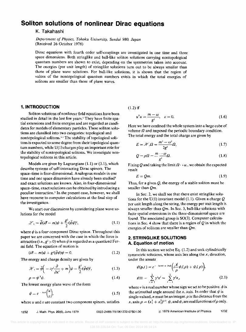
FIG. I. E,=.(g'/rr)E, and Q,=.(mg'/rr)Q, for solutions of (2.6) and (2.7) (p= + I).

K. Takahashi 1235

This article is copyrighted as indicated in the article. Reuse of AIP content is subject to the terms at: http://scitation.aip.org/termsconditions. Downloaded to IP:

128.59.226.54 On: Tue, 09 Dec 2014 06:14:14

2!

I

- ___ 09

_'--- ________________ 1 ______ ~ __ " _____ ~ __ ~ _____ _

° 1 2 3 X 4

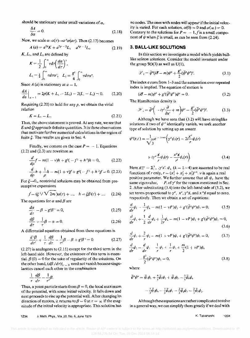
FIG. 2. (a) (g'/m),p \band (b)(g'/m)~,pforv = 0.5,0.7, and 0.9 (P = + I).

By the same argument used in deriving (2.21), we have the virial relation

K (5) = - 2 V~'l, V~S) = 0,

where

K (s) =!!..- ('xc ZdZ(F dH _ H dF + J.-.FH ), g2 Jo dz dz Z

Thus, the energy (4.4) is expressed as

(4.7)

(4.8)

Now, in solving Eqs. (4.2) and (4.3), we seek solutions which have no radial node. We start with an initial value of F at Z = 0 and investigate numerically whether F and H ap­proach zero at large Z or not. If they do and (4.7) is satisfied simultaneously with appropriate precision, we adopt them as solutions. Calculations were performed by the Runge­Kutta method with precision of about 10-4

• In Fig. 1, we /'0. '"

show the behaviors of Es=(g2/1T)Es and Qs=(g2/1T)mQs vs. A A A""'"

v. In the region v < 1, Es < Qs' and both Es and Qs ap-proach the same value as v.-?1, as expected, which implies that our solutions have lower energies than that of plane wave solutions once Qs is fixed. We illustrate (m/g2)1/1 ttP and (m/g2)¢tP for some values of v in Fig. 2 (a) and (b). It is interesting to note that tP t tP has a peripheral structure for small v while ¢tP is always central. For large v, the quantities 1/1 t 1/1 and ¢1/1 have similar behaviors.

1236 J. Math. Phys., Vol. 20, No.6, June 1979

B. Ball-like solutions The equations to be solved are (3.10) and (3.11). We

again restrict ourselves to the case P = + 1. Furthermore, we can choose tPl and tP2 to be eigenfunctions of say,.IJ

I.I; = (i/2)~jk [yj,y"] l due to the invariance of (3.10) and (3.11) under the operation exp(i/2)wl; on tPk' Let us set .I,tPk = tP k' Then tPk are expressed in a similar manner to (2.4).

After changing variables

z=mr, F= g f, H= g h. Ym Ym

Equations (3.10) and (3.11) become

d -F - (1 + v)H + (P - H 2)H = 0, dz

d 2 -H +-H - (1- v)F+ (F2 _H2)F=0. dz z

The energy and charge are

(4.9)

(4.10)

(4.11)

ioo

41T i oo (dF dH 2 EB = 41T rdr?t'2 = -- z2dz H- - F- --F

o mg2 0 dz dz z

(4.12)

1 l j 0.5 10

/;

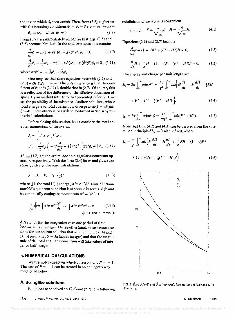
FIG. 3. En=(mg'/61T)EB and Qn=(m'g'/61T)Qnforsolutionsof(3.1O) and (3.II)(P= + I).

K. Takahashi 1236

This article is copyrighted as indicated in the article. Reuse of AIP content is subject to the terms at: http://scitation.aip.org/termsconditions. Downloaded to IP:

128.59.226.54 On: Tue, 09 Dec 2014 06:14:14

r

·-- -_ .. -- ----.----~----.-.---~~- - , (0)

v = 0.5

,------_._---------- --~---~--.----~-~

I (b) 1

~, o . ..----- -- - -- 2 . 3 4

:x:

FIG. 4. (a) (g'/3m)¢at¢d and (b) (g'/3m)¢al/f' fOT v = 0.5, 0.7, and 0.9 (P= + I).

Q8 = 417" f'" rdn(l't¢a = 417" foo z2dz(F2 + H2). Jo m2g2 Jo (4.13)

As in Sec. 4 A, it is useful to derive the virial relation for the

r~-~~--'------T

I 3 i

1

2

/ I

I

(0 )

4 5 6 7

r----~-----~~~-~~T"-\

I 11=0.5 I

/ I (b)

I

o 2 3 4 5 6 7 :x:

FIG. 5. E..:=(g'hr)E, and Q,:=(mg'/rr)Q, for solutions of(2.23) and (2.24) (p= - I).

1237 J. Math. Phys., Vol. 20, No.6, June 1979

r---~------- -- --- -- - ----l

I Os I

I - f, I /00 I .

t\ ~ ,

50 ~

'~

'~

'or -, , L _.....L. __ ~ __ ...L..----L.._~ __ -'-I ---.J

0.5 /.0 /I

FIG. 6. (a) (g'/m)¢ tl,band (b) (g'/m)¢¢for v = 0.5,0.7, andO.9 (P = - I).

present case. The variational principle which produces (4.10) and (4.11) is 8L 8 = 0 with v fixed, where

L8 = 217" foo Z2dZ(F dH _ H dF + l:..FH - (l - v)F2 mg2 Jo dz dz z

/00

50

/0

Q. -- t.

- .. --- ~l

I

I L-.~_~_~~ __ .L....._~ ___ .J

0.5 /.0

(4.14)

FIG. 7. En:=(mg'/6rr)EB and On:=(m'g'/6rr)Qn for solutions of(3. 10) and (3.II)(P = - I).

K. Takahashi 1237

This article is copyrighted as indicated in the article. Reuse of AIP content is subject to the terms at: http://scitation.aip.org/termsconditions. Downloaded to IP:

128.59.226.54 On: Tue, 09 Dec 2014 06:14:14

2

J 0 2 :3 4 5 6 7

x

0.5 ( b)

0

0 2 :3 4 5 6 7 X

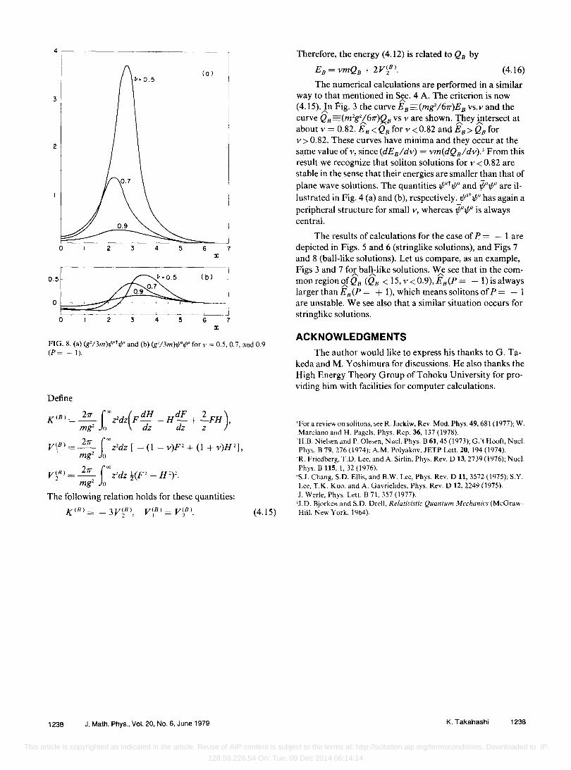
FIG. 8. (a) (g'/3m)l/I't¢" and (b) (g'/3m)¢Q¢" for v = 0.5, 0.7, and 0.9 (p= - 1).

Define

K(B)= 2rr ("'Z'dz(p dH _HdP +2..PH ), mg' Jo dz dz z

ViB) = 2rr (00 z'dz [ _ (1 _ v)P + (1 + v)H'], mg' Jo

viB) =.l:!!...- f'>CO z'dz !(P _ H')'. mg' )0

The following relation holds for these quantities:

K(B)= -3viB), V\B) = ViB). (4.15)

1238 J. Math. Phys., Vol. 20, No.6, June 1979

Therefore, the energy (4.12) is related to QB by

EB = vmQB + 2ViB). (4.16)

The numerical calculations are performed in a similar way to that mentioned in Sxc. 4 A. The criterion is now (4.15). In Fig. 3 the curve E B (mg' /6rr)E B vs. v and the curve QB (m'g'/6rr)QB vs v are shown. They intersect at about v = 0.82. iB < QB for v < 0.82 and iB> QB for v> 0.82. These curves have minima and they occur at the same value of v, since (dEB/dv) = vm(dQB/dv).' From this result we recognize that soliton solutions for v < 0.82 are stable in the sense that their energies are smaller than that of plane wave solutions. The quantities if;at if;G and lifif;a are il­lustrated in Fig. 4 (a) and (b), respectively. if;Gt I/P has again a peripheral structure for small v, whereas ¢Gif;G is always central.

The results of calculations for the case of P = - 1 are depicted in Figs. 5 and 6 (stringlike solutions), and Figs 7 and 8 (ball-like solutions). Let us compare, as an example, Figs 3 and 7 fo;:. bal,klike solutions. W~ see that in the com­mon region ofQB (QB < 15,v<0.9),EB(P= -1)isalways larger than iB(p = + 1), which means solitons of P = - 1 are unstable. We see also that a similar situation occurs for stringlike solutions.

ACKNOWLEDGMENTS

The author would like to express his thanks to G. Ta­keda and M. Yoshimura for discussions. He also thanks the High Energy Theory Group of Tohoku University for pro­viding him with facilities for computer calculations.

'For a review on solitons, see R. Jackiw, Rev. Mod. Phys. 49, 681 (1977); W. Marciano and H. Pagels, Phys. Rep. 36,137 (1978).

'H.B. Nielsen and P. Olesen, Nucl. Phys. B 61, 45 (1973); G.'t Hooft, Nucl. Phys. B 79,276 (1974); A.M. Polyakov, JETP Lett. 20,194 (1974).

'R. Friedberg, T.D. Lee, and A. Sirlin, Phys. Rev. D 13, 2739 (1976); Nucl. Phys. B 115, 1,32 (1976).

'S.J. Chang, S.D. Ellis, and B.W. Lee, Phys. Rev. D 11, 3572 (1975); S.Y. Lee. T.K. Kuo, and A. Gavrielides, Phys. Rev. D 12. 2249 (1975).

'J. Werle, Phys. Lett. B 71,357 (1977). 'J.D. Bjorken and S.D. Drell. Relativistic Quantum Mechanics (McGraw-· Hill. New York. 1964).

K. Takahashi 1238

This article is copyrighted as indicated in the article. Reuse of AIP content is subject to the terms at: http://scitation.aip.org/termsconditions. Downloaded to IP:

128.59.226.54 On: Tue, 09 Dec 2014 06:14:14