Copyright

By

Rohan Ram Mahadik

2011

The Thesis committee for Rohan Ram Mahadik

Certifies that this is the approved version of the following thesis:

Harvesting wind energy using a galloping piezoelectric beam

APPROVED BY

SUPERVISING COMMITTEE:

Supervisor: ________________________________________

Jayant Sirohi

________________________________________

Jeffrey Bennighof

Harvesting wind energy using a galloping piezoelectric beam

by

Rohan Ram Mahadik B.Tech

Thesis

Presented to the Faculty of the Graduate School

of the University of Texas at Austin

in Partial Fulfillment

of the Requirements

for the Degree of

Master of Science in Engineering

The University of Texas at Austin

May 2011

Dedicated

To My

Sister, Rucha and my Parents

v

Acknowledgements

I would like thank Dr.Jayant Sirohi, my advisor, for guiding me so well during

the entire period of my research. He has been a mentor at every point of time in

my Master‘s program. His criticism helped me in improving over my mistakes.

His attittude towards understanding me as student, helping me come up with a

solution, helped a lot. The research carried out as a part of the thesis, would not

have been possible without his supportive nature and continual guidance. I

realized the importance of fundamentals and the need of strong base in one‘s area

of study while working with him. Secondly, I would like to thank my sister,

Rucha, and my parents for being so supportive. I would also like to thank my

friends from Bangalore, India, namely, Ghanshyam Lalwani, Pankaj Patel and

Jayesh Rathod who supported me in all situations, before I joined my Master‘s

program at University of Texas at Austin. All my friends from Austin have been

truly amazing and supportive during my entire stay, with a special mention for

Mithun, Tamanna, and Tushar. I would also like to acknowledge Jerome Sicard,

my colleague, for being helpful in the lab, at times, during my Master‘s program.

Special thanks to Dr. Jeffrey Bennighof for taking out time to read my thesis and

give me valuable suggestions.

vi

Harvesting wind energy using a galloping piezoelectric beam

By

Rohan Ram Mahadik, M.S.E.

The University of Texas at Austin, 2011

SUPERVISOR: Jayant Sirohi

Galloping of structures such as transmission lines and bridges is a classical

aeroelastic instability that has been considered as harmful and destructive.

However, there exists potential to harness useful energy from this phenomenon.

The study presented in this paper focuses on harvesting wind energy that is being

transferred to a galloping beam. The beam has a rigid prismatic tip body.

Triangular and D-section are the two kinds of cross section of the tip body that are

studied, developed and tested. Piezoelectric sheets are bonded on the top and

bottom surface of elastic portion of the beam. During galloping, vibrational

motion is input to the system due to aerodynamic forces acting on the tip body.

This motion is converted into electrical energy by the piezoelectric (PZT) sheets.

A potential application for this device is to power wireless sensor networks on

outdoor structures such as bridges and buildings. The relative importance of

various parameters of the system such as wind speed, material properties of the

beam, electrical load, beam natural frequency and aerodynamic geometry of the

vii

tip body is discussed. A model is developed to predict the dynamic response,

voltage and power results. Experimental investigations are performed on a

representative device in order to verify the accuracy of the model as well as to

study the feasibility of the device. A maximum output power of 1.14 mW was

measured at a wind velocity of 10.5 mph.

viii

Contents

1. Introduction .............................................................................................. 1

1.1 Galloping........................................................................................... 1

1.2 Energy Harvesting ............................................................................ 6

1.3 Applications .................................................................................... 11

2. Theory of Galloping ............................................................................... 15

2.1 ‗D – Section‘ ................................................................................... 16

2.2 Triangular Section ........................................................................... 20

3. Physical mechanism of the galloping device ......................................... 21

3.1 Device based on D – section ........................................................... 21

3.2 Device based on a triangular section .............................................. 23

4. Analytical Model .................................................................................... 28

4.1 Structural model: ............................................................................. 28

4.2 Aerodynamic model: ....................................................................... 33

4.2.1 Galloping device (I) based on D-section ..................................... 33

4.2.2 Galloping device (II) based on equilateral triangular section ..... 34

4.3 Solution procedure: ......................................................................... 35

5. Experimental Set up for model verification ........................................... 37

ix

5.1 Galloping device (I): D – Section ................................................... 37

5.2 Galloping device (II): Triangular section ....................................... 39

6. Results and Discussion ........................................................................... 45

6.1 Galloping device (I): D – Section ................................................... 45

6.2 Galloping device (II): Triangular Section ....................................... 52

7. Summary and Conclusion ...................................................................... 57

8. References .............................................................................................. 60

VITA ............................................................................................................... 64

x

List of Tables 1-1 Comparison of currently available vibration energy harvester products …... 10

1-2 Summary of wireless sensor technology applications ……………….......... 13

5-1 Properties of Galloping device (I) having tip body with D-section ……….. 39

5-2 Accelerometer Specifications ……………………………………………… 43

5-3 Properties of Galloping device (II) having tip body with equilateral triangular

section ……………………………………………………………...................... 44

6-1 Results for galloping device (II) ……………………………………............ 55

xi

List of Figures

Figure 1-1: Schematic of negatively damped oscillation .................................................... 2

Figure 1-2: Transmission line section [2] .......................................................................... 4

Figure 1-3: Humdinger energy [11] windbelt device ........................................................ 11

Figure 2-1: Forces on a D-section in an incident wind ..................................................... 16

Figure 2-2: Cl and Cd plots for a D-section, from Ratkowski [28]. The angle of attack is

defined with respect to the flat face. ........................................................................ 18

Figure 2-3: Parameters of an isosceles triangular section body subjected to incident wind

velocity ..................................................................................................................... 20

Figure 3-1: Schematic of galloping device (I) showing galloping mechanism and change

in instantaneous angle of attack α ............................................................................ 21

Figure 3-2: Stability diagram in the angle of attack-main vertex angle plane (α, β).

Numbers on the curves indicate the value of (dCldα Cd ) Note that the stability

diagram is symmetric with respect to α = 180o [30] ................................................ 24

Figure 3-3: Cl , Cd plot for an equilateral triangular section (vertex angle β = 60o) [30] .. 26

Figure 3-4: Schematic of galloping device (II) with a triangular section tip body attached

to an elastic beam, subjected to incident wind speed ............................................... 27

Figure 4-1: Schematic of device (I) showing spatial discretization over tip body of D-

section ...................................................................................................................... 33

Figure 4-2: Schematic of beam geometry ......................................................................... 35

Figure 4-3: Block diagram of solution procedure in MATLAB Simulink ....................... 36

Figure 5-1: Experimental set up showing bimorph beam and attached wooden bar of D

section ...................................................................................................................... 38

xii

Fig 5-2: Schematic of the accelerometer position on the tip of the beam to measure

acceleration in X and Y direction ............................................................................. 40

Figure 5-3: Schematic of beam tip displacement .............................................................. 40

Figure 5-4: Experimental set up in the subsonic wind tunnel at the university, showing

two elastic beams attached to a triangular section tip body. .................................... 42

Figure 5-5: A photograph capturing the oscillations due to galloping instability of a tip

body with equilateral triangular section attached to elastic beams. Location:

Subsonic wind tunnel at the University of Texas at Austin ..................................... 43

Figure 6-1: Measured voltage generated by the piezoelectric sheets, 0.7MΩload

resistance at wind velocity of 9.5 mph ..................................................................... 45

Figure 6-2: Measured voltage generated by the piezoelectric sheets at steady state,

0.7MΩload resistance at wind velocity of 9.5 mph ................................................ 46

Figure 6-3: Measured impulse response of the beam, with electrodes open-circuited. .... 47

Figure 6-4: Comparison of measured and predicted voltage at steady state, 0.7 MΩload

resistance at wind speed of 8 mph. ........................................................................... 48

Figure 6-5: Transient response of the beam as predicted by analysis, at incident wind

speed of 8.6 mph, and 0.7 MΩ load resistance ........................................................ 48

Figure 6-6: Comparison of measured and predicted steady state voltage, as a function of

load resistance, at wind speed of 8.5 mph ................................................................ 49

Figure 6-7: Comparison of measured and predicted steady state voltage as a function of

incident wind velocity, for 0.7 MΩ load resistance ................................................. 50

Figure 6-8: Measured power as a function of load resistance, at 8.5 mph wind speed ..... 50

xiii

Figure 6-9: Measured and predicted output power versus wind velocity, 0.7 MΩ load

resistance. ................................................................................................................. 51

Figure 6-10: Accelerometer voltage signal measuring X (blue line) and Y (green line)

acceleration at the tip of the beam, at incident wind speed of 7 mph ....................... 53

Figure 6-11: Transient tip displacement response of galloping device (II) subjected to

incident wind speed of 6.4 mph ............................................................................... 54

Figure 6-12: Steady state tip displacement response of galloping device (II) subjected to

incident wind speed of 6.4 mph ............................................................................... 55

1

1. Introduction

1.1 Galloping

Galloping of a structure is characterized as a phenomenon involving low

frequency, large amplitude oscillations normal to the direction of incident wind.

Typically, it occurs in lightly damped structures with asymmetric cross sections.

Galloping is caused by a coupling between aerodynamic forces acting on the

structure and the structural deflections.

Consider a body within a fluid at rest. Let the body be a flexible structure

having some stiffness. If it is excited by an impulse forcing, it will undergo

oscillation but eventually, the structural damping and the viscosity of the

surrounding fluid will attenuate the oscillations and the body will come to rest.

However, due to interaction with fluid, there is a possibility that the body may be

acted upon by forces with an appropriate phasing. An appropriate phasing would

mean that the forces generated are acting at a point in the periodic cycle when

they do not attenuate but enhance the disturbance caused. In such a case, the body

might continue to oscillate or even amplify its oscillations. Such a behavior

occurs when the body is unstable. The state of being unstable can be defined as

the state when the forces act in a phasing so as to increase oscillation amplitude.

This behavior is called galloping. Galloping can be called as self-excited

2

oscillations. It can be translational or torsional in nature. The thesis discusses

translational galloping only.

Den Hartog [1] explained the phenomenon of galloping for the first time in

1934 and introduced a criterion for galloping stability. He was the first to explain

how disturbances can also cause self-excited vibrations. In self-excited vibration

the alternating force that sustains the motion is created or controlled by the

motion itself; when the motion stops, the alternating force disappears. In an

ordinary forced vibration, the sustaining alternating force exists independently of

the motion and persists even when the vibratory motion is stopped. Another way

of looking at this matter is by defining self-excited vibration as vibration with

negative damping.

Figure 1-1: Schematic of negatively damped oscillation

A system with negative damping is dynamically unstable. The oscillations

grow or magnify in amplitude with time as shown in Fig 1-1. On the other hand, a

Time

Oscill

atio

n (

dis

pla

ce

me

nt)

3

system with positive damping is dynamically stable. The oscillations reduce in

amplitude with time.

Den Hartog explained how self excited oscillations occur due to winds with

the help of an example about galloping of ice-covered electrical transmission

lines. Transmission lines have been observed to vibrate with large amplitudes

during winter weather conditions. This phenomenon has been observed in cold

countries like Canada and Northern part of the U.S. during winter when a strong

transverse wind is blowing. The frequency of vibration has been observed to be

same as the natural frequency of the transmission line system. The cross section

of the transmission line cable is generally circular. Circular section being

symmetric is dynamically stable if transverse wind is blowing. There is no

disturbance force acting on it. However, when ice sleet is formed underneath the

transmission line, the circular cross section now converts into an asymmetric

shape as shown in Fig 1.2. Such asymmetric shapes are prone to exhibit galloping.

Chabart and Lilian [2] have conducted galloping experiments in wind tunnel on

scaled bodies to replicate galloping of transmission lines having ice-sleet on them.

4

Figure 1-2: Transmission line section [2]

There are various asymmetric shapes that are prone to galloping. Studies have

been carried out in past on different cross-sections, such as, rectangular,

prismatic, D-section and triangular. Significant research has also been done to

study various other parameters that influence galloping of structures due to wind.

Alonso et al. [3] conducted experimental measurements on a triangular cross

section undergoing galloping due to wind. Alonso et al. demonstrated

experimentally the dependence of angle of attack* on occurrence of galloping. He

determined aerodynamic coefficients, such as lift and drag, over a range of angle

of attack from 0 to 180 degrees by means of wind tunnel experiments. This was

helpful in predicting the unstable region in that range, for an isosceles triangular

section subjected to transverse wind.

* Angle of attack: Angle between wind velocity incidence and mean chord of a section undergoing

galloping at an instant of time.

5

The vertex angle of an isosceles triangular section also decides the instability.

Kazakevich and Vasilenko [4] have investigated and found dependence of

galloping amplitude on wind velocity by a means of a closed form analytical

solution for a rectangular section. They showed galloping begins only beyond a

certain wind velocity, called as critical wind velocity. It is the minimum wind

velocity required to initiate galloping and varies from section to section. Using

their model, critical wind velocity can be predicted for rectangular sections. They

have also discussed how breadth to height ratio affects the stability of rectangular

section. From this example and the previous example of isosceles triangular

section, it is seen that geometry plays a significant role in galloping. Experimental

results obtained by Laneville et al. [5] on a D-section exposed to wind flow show

that it is highly prone to galloping at higher angles of attack. Thus, this past

research identifies influence of parameters such as geometry of the section, wind

velocity and angle of attack, on galloping stability.

The self-excited structural oscillations are a form of available mechanical

energy. They can be beneficial if harvested into useful form. The following

section discusses the concept of energy extraction, and the currently available

devices that can extract energy available from different energy sources, into

useful form.

6

1.2 Energy Harvesting

Energy harvesting is the process of converting available energy from one form

to another useful form. As a part of this thesis, conversion of structural vibrations

to useful electrical energy has been discussed. There are several ways to harvest

energy. The methods discussed here, relevant to this study, are:

1. Harvesting energy from base-excited vibration

2. Harvesting energy from flow induced vibrations

3. Harvesting energy from flutter due to wind flow

Energy harvesting from base-excited vibration is done by conversion of

available ambient vibration at source into electrical energy. The source of ambient

vibration, as an example, can be operating machinery. The method of conversion

involves using smart materials such as piezoelectric (PZT) materials.

Piezoelectricity refers to generation of electricity when such smart materials are

subjected to mechanical stress. It is observed in many naturally occurring crystals.

Most piezoelectric materials are crystalline in nature; they can be either single

crystals or polycrystalline. The unit cell of these crystals possess a certain degree

of asymmetry, leading to separation of positive and negative charges that results

in permanent polarization. The effect was first predicted and then experimentally

measured by the Curie brothers, Pierre and Jacques, in 1880. This effect is also

7

known as the direct piezoelectric effect which means electric polarization

produced by mechanical stress, is directly proportional to the applied stress. In

other words, if stress is applied to the piezoelectric material, a proportional

electrical charge is produced. This charge can be extracted by means of an

electrical circuit.

. Piezoelectric materials have found wide application as low power generators.

In the majority of these applications, the energy harvester is attached to a

structure, and it extracts energy from ambient vibrations by operating as a base-

excited oscillator. Several analytical models have been proposed to quantify the

electrical energy that can be generated. Sodano et al. [6] developed a model of a

piezoelectric beam undergoing base-excited vibrations, to predict the dynamic

response, power, voltage and current output. The model uses energy methods to

develop constitutive equations for a bimorph piezoelectric energy harvesting

beam. Umeda et al. [7] investigated the electrical energy generated by a metal ball

falling on a plate with a bonded piezoelectric sheet, and proposed an electrical

equivalent circuit that described the conversion of potential energy into electrical

energy in the piezoelectric material. Roundy et al. [8] discussed the operation and

analytical modeling of a base-excited energy harvester consisting of a

piezoelectric bimorph with a lumped mass attached to its tip. A relationship for

power output as a function of input vibration amplitude and frequency was

developed. Ottman et al. [9] designed optimal power conditioning electronics for

a piezoelectric generator driven by ambient vibrations. Ajitsaria et al. [10]

8

developed mathematical models for the voltage generated by a bimorph

piezoelectric cantilever beam, using three different approaches.

Several academic research institutions and commercial manufacturers are

involved in the design and manufacturing of energy harvesters excited by ambient

vibration. Some of them are listed here. They include IMEC and the Holst Centre

– Eindhoven Netherlands, Massachusetts Institute of Technology at Boston,

Georgia Institute of Technology at Atlanta, University of California at Berkeley,

Southampton University in U.K, PMG Perpetuum, and National University of

Singapore.

IMEC & Holst centre [10] has developed a micro-machined energy harvester

which delivers 60μW power at an input acceleration of 2g and resonance

frequency equal to 500Hz. It consists of a piezoelectric capacitor formed by a Pt

electrode made of an aluminium-nitride (Al-N) layer and a top Al electrode. The

capacitor is fabricated on a cantilever beam which has a tip mass. When the

harvester vibrates, the mass on the cantilever causes the piezoelectric layer to

bend, inducing an electrical power. The Al-N layer has advantage over

piezoelectric material that it can be made by a simpler deposition process.

AdaptivEnergy [12] designs, manufactures and markets energy harvesting power

solutions. The company provides a range of products for different operating

frequencies and required output DC voltage. The product module is designed to

operate at random vibration environments. In its present form and application

space, the module can power microelectronic devices such as microcontrollers,

9

wireless switches, wireless sensor networks and ActiveRFID tags in

transportation and industrial environments. Environment such as bridges, roads,

tunnels, motors, compressors, pumps, helicopter and power transformers are used

as vibration source by these energy harvesting modules. Advanced Cerametrics

Incorporated – ACI‘s Harvestor line of products [13] produce electrical power

from ambient vibration energy by means of piezoelectric fiber composites (PFC)

and their proprietary efficient power management circuits. The working principle

is that the piezo-ceramics bend due to input vibration and electrical charge is

produced. Their latest power module product named ‗Harvester–III‘ is light

weight, compact in size, with different models available to operate at different

excitation frequencies of vibration. Mide Technology Corporation [14], located in

Cambridge, Boston, Massachusetts, is another manufacturer of wireless

vibrational energy harvesters named ‗Volture‘. PMG Perpetuum [15] , located in

Southampton, U.K., is a leading producer of vibration energy harvesting products.

All the above studies targeted piezoelectric energy harvesters based on ambient

structural vibrations. As a result, these devices are inherently limited to relatively

low power outputs. Table 1.1 gives a comparison of currently available vibration

energy harvester products.

10

Company Dimension

(mm3)

Operating

Vibration

frequency

(Hz)

Output

Volt

DC

Acceleration

amplitude

‗g‘ value

Power

output

(mW)

Capacitive

storage

(μF)

AdaptivEnergy

Joule thief

module

60 x 25 x 25 14 3.6 0.075 0.18 66

ACI -Harvester

–III H30

165 x 35 x 40 30 3.0 3 -- 100

ACI: Harvester

– III H60

125.3 x 50 x

22.5

60 3.0 3 -- 100

ACI: Harvester

– III H120

125.3 x 50 x

22.5

120 3.0 3 -- 100

ACI: Harvester

– III H220

110.2 x 56 x

23.5

220 3.0 3 -- 100

Mide: Volture

PEH25w

92 x 43.8 x 9.9 75-175 N.A. 0.35-1.8 3 – 31

at 50 Hz

0.2

Perpetuum:

PMG17 – 100

55 dia, 55

height

100 4.5 0.025 - 1 1 – 45 N.A.

Table 1-1 Comparison of currently available vibration energy harvester products.

There have been limited studies in past on harvesting energy from

aerodynamic instabilities [16]. Wang and Ko [17] have carried out studies to

harvest energy from flow-induced vibrations. Their base-excited energy harvester

converts flow energy obtained from pressure excitation into electricity by

oscillation of a piezoelectric sheet. They generate an output power of 0.2μW at an

excitation frequency of 26 Hz. Barrero-Gil et al. [18] theoretically investigated

the feasibility of energy harvesting from structures undergoing galloping. They

represented the sectional aerodynamic characteristics using a cubic polynomial

and obtained an expression for the harnessable energy. Specific methods for

energy extraction were not discussed. Robbins et al. [19] investigated the use of

11

flexible, flag-like, piezoelectric sheets to generate power while flapping in an

incident wind.

Energy harvesting from flutter phenomenon has also become known. Self-

excited oscillations or flapping of a tensioned membrane incident to wind flow

can be referred to as flutter. Humdinger wind energy [20] is a recently formed

company that researches and develops windbelt generator. Windbelt is a

harvesting device that uses a tensioned membrane undergoing a flutter oscillation

to extract energy from the wind. It uses electromagnets to generate electricity

from the flutter of the membrane.

Figure 1-3: Humdinger energy [11] windbelt device

1.3 Applications

The availability of low-power micro-sensors, actuators, and radios is enabling

the application of distributed wireless sensing to a wide range of applications such

12

as smart spaces, medical applications, and precision agriculture [21][22]. Sensor

networks can remotely report temperature, moisture and sunlight intensity in

farms, to a central computer. Wang et al. [23] have described a wireless sensing

prototype system specially designed for structural monitoring of a bridge.

Mainwaring et al. [24] have provided an in-depth study of applying wireless

sensor networks to real-world habitat and environmental monitoring such as

monitoring seabird nesting environment in an ecological reserve. They describe

the power requirement for each node to be 6.9mAh per day. The ‗eKo system‘ by

Crossbow Technology Inc. [25] is a similar application of outdoor wireless

sensing in fields which however, uses a miniature solar panel for powering the

sensor network . Evans and Bergman [26] are leading a USDA research group to

study precision irrigation control. Wireless sensors were used in the system to

assist irrigation scheduling using combined on-site weather data, remotely sensed

data and grower preferences. Table 1.2 gives a summary of wireless sensor

technology manufacturers and their respective applications.

13

Company Sensor Technologies Sensor Application

Crossbow Motes: Mica2, Mica2Dot, MicaZ

Gateway nodes: Stargate,MIB600

Interface board: MIB600 Ethernet,

MIB510 Serial, MIB520 USB

Seismic structural monitoring,

indoor/outdoor environmental

monitoring, security protection

and surveillance monitoring,

inventory monitoring, health

monitoring

Sentilla

(Moteiv)

Motes: T-mote sky

Gateway nodes:T-mote Connect

Indoor and outdoor monitoring

applications

Dust Networks SmartMesh-XT motes: M1030,

M2030, M2135

SmartMesh-XT manager: PM1230,

PM2030, PM2130

Building automation monitoring,

industrial process monitoring,

and security and defense

monitoring

Millenial net MeshScape 916 MHz and 2.4

MHz: mesh node, mesh gate, end

nodes

Mesh485: mesh sub-based router,

mesh router, and mesh bridges

Building monitoring and

industrial process monitoring

Sensicast Sensicast EMS and RTD nodes

Sensicast gateway bridge, mesh

Router

Industrial monitoring of

temperature and energy

Table 1.2: Summary of wireless sensor technology applications [27]

Most of the wireless sensor network systems are powered by batteries.

Replacement of depleted batteries for large network systems is expensive, often

impractical and environmentally unfriendly. Hence, the use of energy harvesting

methods to power the sensors on-site can be beneficial. Energy harvesting reduces

dependency on battery power. The harvested energy may be sufficient to

eliminate battery completely. It reduces maintenance costs and eliminates battery

replacement labour. This is especially important in outdoor locations such as

14

inaccessible terrain, geological parks where human interaction is minimum.

Powering the wireless sensors, located outdoors, by means of wind energy is a

practical alternative to battery power sources.

A piezoelectric energy harvesting device based on a galloping cantilever beam

is described in the present work. Such a device has the primary advantages of

simplicity and robustness, and could be collocated with the wireless sensors to

provide a source of renewable wind energy.

15

2. Theory of Galloping

Galloping theory for D-section and triangular section is discussed in the

following sub sections. The motivation for performing research in this area came

from a simple galloping experiment. The apparatus is shown in Fig 2-1. A semi

circular wooden bar (12 inch long and 1 inch in diameter) is suspended by four

springs. The natural frequency is kept low (<10 cycles per second). When the

apparatus is placed in front of an axial fan, the bar builds up vibrations. Energy is

being added into the system and the bar can sustain its oscillations over time,

inspite of structural damping of the system. Galloping is dependent on the shape

and size of the body subjected to transverse air flow. In the following sections, the

theory of galloping for two geometrical cross sections has been discussed in

detail.

Figure 2-1: Schematic of a galloping beam experiment in lab

16

2.1 ‘D – Section’

Consider a prismatic structure with a D-shaped cross-section mounted on a

flexible support, exposed to incident wind with a velocity V∞ along the x-

direction as shown in Figure 2-1. . Initial perturbations generated by the vortices

shed from the D-section result in small, periodic oscillations normal to the

direction of incident wind. Let the section be moving downward with a velocity

(defined as positive in the positive y-direction). The instantaneous angle of attack

α is given by:

α =

= -

(1)

where ‗Va‘ is the apparent velocity of the air, equal in magnitude and opposite

in direction to Va is defined as positive in y direction. α depends upon the

velocity of the galloping body and on the free air flow velocity.

Figure 2-1: Forces on a D-section in an incident wind

L

Dα

y

x

Va

V∞

Vrel

Incident wind

velocity

b

17

It is seen that α depends upon the velocity of the galloping body as well as

on the incident velocity. The quasi-steady lift force L and drag force D (per unit

length) on the section are given by:

L =

(2)

D =

(3)

where b is the characteristic length normal to incident flow (chord of the D-

section), ρ is the air density, and Cl, Cd are the sectional lift and drag coefficients

respectively. Previous research has shown that it is sufficient to include only

quasi-steady aerodynamic forces in the analysis, because the characteristic time

scale of the system (b/V∞) is much smaller than the galloping time period [18] .

The components of the lift and drag along the y-direction give the

instantaneous excitation force per unit length Fy as:

(4)

where the coefficient of the force in the y-direction, CFy, is given by:

[ ] (5)

Typical 2D (two-dimensional) sectional lift and drag coefficients for a D-

section were measured by Ratkowski [28], and are shown in Fig. 2-2. Note that

the angle of attack (plotted along the x-axis) is defined as the angle between the

incident wind and the flat face of the D-section. For a D-section oriented as

shown in Figure 1, the angle of attack is close to 90°. In this region, it is seen that

18

the lift coefficient Cl is approximately linear and has a negative slope. The drag

coefficient Cd is approximately constant.

Figure 1-2: Cl and Cd plots for a D-section, from Ratkowski [27]. The angle of attack is

defined with respect to the flat face.

Let the flexible support structure have an effective mass per unit length of ‗m’,

damping factor ‗‘ and stiffness ‗m ‘. The equation of motion of the D-section

mounted on the flexible support is basically that of a linear spring mass damper

oscillator with a forcing term ‗ ‘ that is a function of angle of attack α, and

therefore depends on the velocity of the D-section. The equation of motion is

given by:

[ n n ] (6)

For small displacements from the equilibrium position (α=0),

-0.4

-0.2

0

0.2

0.4

0.6

0.8

1

1.2

0 10 20 30 40 50 60 70 80 90Aer

od

yn

amic

co

effi

ecie

nt

Angle of attack, deg

Cl

Cd

19

(7)

where the dependence of the force coefficient CFy with angle of attack is given

by:

(

dCl

dα Cd) (8)

Hence, for small α, Eq.(6) can be written as:

[ n n ]

(dCl

dα Cd)

(9)

Equation (9) represents the general equation of motion governing galloping of

the structure. It is seen that the forcing term acts as an additional damping due to

its dependence on . Unstable oscillations, i.e., galloping, occur when the

effective damping of the system becomes negative. For low values of ,the

condition for galloping to occur can be written as:

(dCl

dα Cd ) 0 (10)

Equation (10) is known as the Den Hartog criterion 0 and can be used to

estimate when galloping will occur on any given structure. This criterion depends

only on the sectional aerodynamic coefficients; specifically, galloping occurs

when

α (11)

From Figure 2-2, it is seen that this condition is satisfied for the D-section

when the incident wind is perpendicular to the flat face. The negative damping

20

factor ‗’ during galloping condition indicates that energy is extracted by the

structure from the air stream. This energy can be harvested and used as a power

source.

2.2 Triangular Section

Similar to a D-section, a triangular section also undergoes galloping

oscillation when subjected to wind. Alonso et al. [29] discuss galloping instability

of triangular section bodies in particular. Equations (1) to (11) are valid also for

the triangular section arrangement shown in Fig 2-3. For an isosceles triangular

section, let αo be the angle of attack with respect to incident wind velocity, and β

be its main vertex angle. β is a key geometrical parameter affecting the sectional

aerodynamic characteristics and hence the galloping stability.

Figure 2-3: Parameters of an isosceles triangular section body subjected to incident wind

velocity

The studies conducted by Alonso et al. [29] helped in a second choice of a

triangular section to build the galloping device.

21

3. Physical mechanism of the galloping device

Two Galloping devices are investigated to demonstrate energy harvesting

capabilities. Galloping device (I) is made of a body having D-section with flat

face facing the incoming wind. Galloping device (II) is made of a body having

triangular section with flat face facing the incoming wind. These devices are

described in the following sections 3.1 and 3.2.

3.1 Device based on D – section

Figure 3-1: Schematic of galloping device (I) showing galloping mechanism and change in

instantaneous angle of attack α

Free Air

stream

Oscillating

motion

Aluminium

Cantilever beam

D section

Strip of Piezoelectric

material

+ -

A.C.

Voltage

generated

+ -

FRONT

VIEWSIDE

VIEW

0

+-

α

1

3

2,4

3

24

1

y

22

A galloping device (I) developed as a part of this study consists of a rigid

wooden bar 235 mm long, having D-shaped cross section of 30 mm diameter. The

bar is attached to the tip of an aluminum cantilever beam. The aluminum beam

size (in mm) is 90 x 38 x 0.635. The schematic of the device (I) is shown in Fig.

3-1. The beam is initially held at rest. The direction of incident wind is normal to

the flat surface of the D-section, which corresponds to an angle of attack of 90° as

defined in Fig 3-1. For angles of attack in this range, the lift curve slope of the D-

section is negative, and the Den Hartog criterion is satisfied. As a result, the D-

section is prone to galloping. Initial perturbations are caused by vortex shedding

and the D-section begins to gallop in a direction transverse to the plane of the

beam. The resulting oscillatory bending displacement of the beam progressively

increases in magnitude as energy is transferred from the incident wind to the

structure. Piezoelectric sheet elements (PZT) bonded to the top and bottom

surface of the aluminum beam generate an alternating voltage in response to the

bending induced by the galloping D-section. In a practical wind energy harvester,

the generated electrical energy would be stored or used to power other devices,

however, in the present study, the voltage is simply discharged across a load

resistance.

The load resistance across the piezoelectric sheets dissipates energy in the

form of Ohmic heating and hence, acts as an additional positive damping on the

system. Therefore the amplitude of oscillation of the beam increases till a steady

state is reached, wherein the energy extracted from the incident wind is exactly

23

equal to the energy dissipated across the load resistance. In this steady state, the

amplitude of oscillation remains constant. For a given incident wind velocity, the

induced angle of attack is a function of the beam tip displacement, oscillation

frequency, tip slope and location along the tip body.

3.2 Device based on a triangular section

This section examines the effects of cross-sectional shape and angle of attack

on transverse galloping stability of a triangular section. Published data on

triangular section are used to determine its geometry and aerodynamic

characteristics for maximum energy extraction. Alonso and Meseguer [30] have

analyzed the effect of main vertex angle β and angle of attack α on galloping

stability of triangular section bodies. Their study identified unstable regions in the

(α, β) plane. Figure 3-2 shows these zones. Alonso and and Meseguer [30] tested

nine triangular prisms having sharp edges, the main vertex angle ranging from β =

10o to 90

o in 10 degree increment. Section Cl and Cd data results for these nine

prisms were thus obtained through wind tunnel experiments over a range of 0 to

180o angle of attack. The Den-Hartog criterion (

dCl

dα Cd < 0) is applicable to a

triangular section also and it is evaluated in the (α, β) plane. When plotted it

results in Fig 3-2. Unstable regions can be identified where the Den-Hartog

criterion is negative.

24

Figure 3-2: Stability diagram in the angle of attack-main vertex angle plane (α, β). Numbers

on the curves indicate the value of (d l

dα d ) Note that the stability diagram is

symmetric with respect to α = 180o [30]

Galloping of triangular cross-section bodies is more favourable when the base

of the triangle is facing the incident wind stream. Figure 3-2 shows how the

unstable zones lie around α = 60o and α = 180

o. The aerodynamic drag coefficient

(Cd in (dCl

dα Cd )) is larger when there is a separation of flow behind the triangular

25

cross-section. As the main vertex angle β increases, separation of flow increase,

and thus the magnitude of drag force also increases. A large angle β is

undesirable, since it reduces the value of (dCl

dα Cd ) term. Although the unstable

zone close to α = 180o becomes wider as value of β increases, the value of

(dCl

dα Cd ) term reduces with larger β. For very small angle β, the instability

region near α = 60o and α = 180

o is narrow. Hence, very small angle β is

undesirable. For β < 60o, although (

dCl

dα Cd ) is more negative in value, the

unstable range of α near 180o is narrow. Galloping motion depends on angle of

attack α and occurs for only a certain range of α. A narrow unstable range of α

would be undesirable. On the other hand, for β > 60o, the unstable range of α near

180 o

is wide, however, (dCl

dα Cd ) is less negative in value and is close to zero.

But a more negative value is desirable to maximise galloping amplitude. Hence,

as a trade off, an equilateral triangular section (β = 60o) is selected as the best

preferred geometry to produce galloping. Figure 3-3 shows the Cl, Cd plot for

equilateral (β = 60o) triangular section. At α = 60

o, the base of the triangular

section is facing the incoming wind stream, and such an orientation is desirable

for galloping to occur. The range of α in these regions for instability is wide. The

negative Cl slope region ranges from α = 25o to 95

o, where α = 60

o being the mean

position. The galloping will continue as long as the angle of attack stays within

this region.

26

Figure 3-3: Cl , Cd plot for an equilateral triangular section (vertex angle β = 60o) [30]

A 2nd

galloping device (II) is developed as shown in Fig 3-4, and it consists of

a 251 mm long tip body with an equilateral triangular section (each side 50 mm)

attached to two elastic beams, 161 mm long each, at both ends. As discussed

before, the base of the triangular section faces the incident wind, implying the

angle of attack αo at mean equilibrium position is 60o.

-1.5

-1

-0.5

0

0.5

1

1.5

2

0 30 60 90 120 150 180

Cl

, C

d

angle of attack (deg)

Cl

27

Figure 3-4: Schematic of galloping device (II) with a triangular section tip body attached to

an elastic beam, subjected to incident wind speed

28

4. Analytical Model

A coupled electromechanical model of the galloping energy harvesting device

is developed from a mechanics based approach, using the coupled

electromechanical energy of the system (see Sodano et al [6] , Lee [31], Nisse

[32]) The goal of the model is to predict the voltage generated by the PZT as a

function of time, for a given incident wind speed, beam geometry and load

resistance. The model consists of two parts: the structural model and the

aerodynamic model. Devices with different tip bodies can be modeled using

different aerodynamic models in conjunction with the same structural model.

4.1 Structural model:

The constitutive equations of a piezoelectric material, relating the strain and

electric displacement D to the mechanical stress , and electric field E are given

by Error! Reference source not found.:

* + *

+ *

+ (12)

where is the compliance matrix, is the matrix of dielectric constants,

and is the piezoelectric coupling matrix. The superscripts E and signify

quantities measured at constant electric field and mechanical stress, respectively.

29

The potential energy of the device consists of terms due to mechanical strain

energy as well as electrical energy, and is given by:

∫

∫

∫

(13)

where the quantity Vp indicates the volume of the piezoelectric element and Vs

is the volume of the base structure. In the case of the device in the present study,

Eq.(13) can be simplified by substituting one-dimensional quantities for stress,

strain, electric field and electric displacement, yielding:

∫

∫

∫

(14)

Because the coupled energy (as opposed to enthalpy) of the system is being

considered, it must be expressed in terms of the basic quantities D and .

Dropping the subscripts and substituting for stress and electric field from the

piezoelectric constitutive equations gives

∫

∫

∫

(15)

where the superscripts D and refer to quantities measured at constant electric

displacement and constant strain, respectively. The electromechanical coupling

coefficient of the piezoelectric, k is given by:

(16)

Note that

(17)

30

(18)

Using the Euler-Bernoulli theory for a beam in bending yields the strain at any

height y from the neutral axis as:

(19)

where is the curvature (v is the vertical displacement in the y-direction).

The beam displacement v can be assumed as:

∑ (20)

where is the row vector of shape functions set to satisfy boundary

conditions, r is the column vector of temporal coordinates of displacement and N

is the number of shape functions included in the analysis. The electric

displacement is related to the charge generated q and the area of the electrodes Ap

by:

(21)

Substituting the above expressions into Eq. 15 yields the potential energy of

the device as:

∫

∫

∫

(22)

The kinetic energy T is given by:

∫

∫

(23)

31

The quantities mtip and Itip correspond to the mass and moment of inertia of the

tip body, respectively. Substituting for the assumed displacements, we get

∫

∫

(24)

The external virtual work done on the system is given by:

(25)

where Ftip and Mtip are the external forces and moments acting at the tip of the

beam, and is the voltage across the electrodes on the piezoelectric sheets. The

governing equations of the system can be derived from the potential energy,

kinetic energy and virtual work either by using Hamilton‘s principle or by

applying Lagrange‘s equations. The governing equations are:

(26)

(27)

In the above equations, the effective mass matrix is given by:

∫

∫

(28)

The effective stiffness matrix is given by:

∫

∫

(29)

A coupling vector can be defined as:

∫

(30)

32

The capacitance of the piezoelectric sheets, Cp is given by (assuming a

uniform cross-section and a piezoelectric sheet of thickness tp):

(31)

In addition, for the present system, the voltage and charge are coupled

together by the load resistance RL connected across the electrodes of the

piezoelectric sheets. This relation can be expressed as:

(32)

Eq.(26) and Eq.(27), in conjunction with the voltage-charge relation given by

Eq.(32) represent a coupled electromechanical model of the power harvesting

device. To account for structural damping, an additonal proportional damping

matrix C is incorporated.

C = α M + β K (33)

where α and β are determined from:

i = 1,2,..N (34)

In the above equation, is the natural frequency of the ith

mode, is the

modal damping, and N is the number of modes (equal to the dimension of the

mass and stiffness matrices). These quantities are measured experimentally from

the impulse response of the beam with an appropriate electrical boundary

condition for the piezoelectric sheets.

33

4.2 Aerodynamic model:

The aerodynamic model will vary for D-section and triangular section. The

right hand side of Eq.(26) represents the forcing function.

4.2.1 Galloping device (I) based on D-section

Figure 4-1: Schematic of device (I) showing spatial discretization over tip body of D-section

The tip of the beam is subjected to aerodynamic force Ftip and tip moment Mtip

that are due to the sectional aerodynamic force Fy integrated over the length L of

the tip body.

∫

∫ [ ]

(35)

∫

(36)

where s is the length coordinate along the tip body. Due to the geometry of the

device, the sectional angle of attack is a function of rate of change of beam tip

displacement, rate of change of beam tip slope and the location of the section

along the tip body. The section angle of attack accounts for the rotation of the tip

body. It is given as:

34

(37)

The sectional lift and drag coefficients were obtained from the data measured

by Ratkowski [28] (Fig. 2-2). Note that the angle of attack αeff required to use

this data is related to the angle of attack in Eq.(37) by:

(38)

4.2.2 Galloping device (II) based on equilateral triangular section

The geometry of the galloping device (II) [Fig. 3-6] is such that, every cross

section along the length of the triangular tip body is subjected to the same angle

of attack at any given point of time. It implies that the lift force acting at any cross

section of the tip body is same over the entire length of the tip body at any instant

of time. Hence, it is not required to consider for the rotation effect over the length

of the triangular tip body. The calculation of tip aerodynamic force is as follows:

Fy tip (triangular) = ∫

∫ [ ]

(39)

Where Fy is the aerodynamic force per unit length of tip body with triangular

section. The tip aerodynamic force is used as external forcing to determine the

output of the system. There is no moment acting on the tip body.

35

The sectional lift and drag coefficients were obtained from the data measured

by Alonso [30] (Fig.3-4). Note that the angle of attack αeff required to use this

data is related to the angle of attack in Eq.(39) by:

(40)

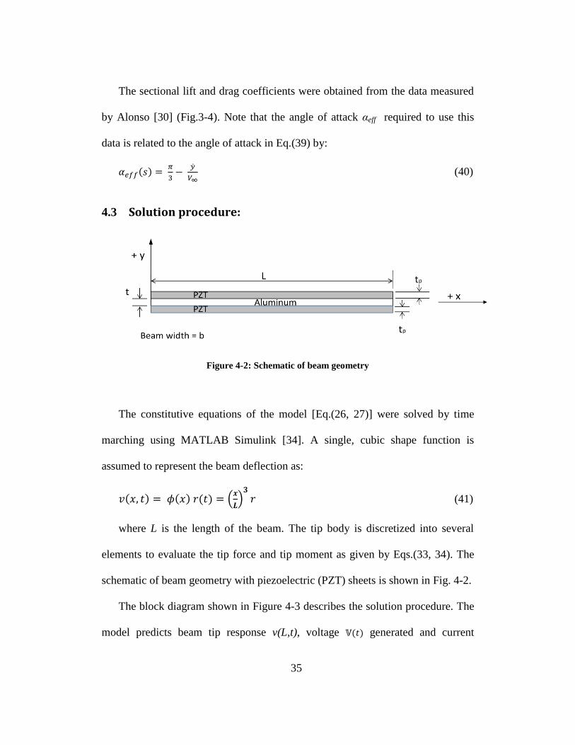
4.3 Solution procedure:

Figure 4-2: Schematic of beam geometry

The constitutive equations of the model [Eq.(26, 27)] were solved by time

marching using MATLAB Simulink [34]. A single, cubic shape function is

assumed to represent the beam deflection as:

(

)

(41)

where L is the length of the beam. The tip body is discretized into several

elements to evaluate the tip force and tip moment as given by Eqs.(33, 34). The

schematic of beam geometry with piezoelectric (PZT) sheets is shown in Fig. 4-2.

The block diagram shown in Figure 4-3 describes the solution procedure. The

model predicts beam tip response v(L,t), voltage generated and current

36

flowing through the load resistance for given values of incident wind velocity,

load resistance and device geometry. Tip bodies of any cross-sectional geometry

can be evaluated by incorporating the appropriate sectional airfoil characteristics

in the form of a table lookup.

Figure 4-3: Block diagram of solution procedure in MATLAB Simulink

37

5. Experimental Set up for model verification

5.1 Galloping device (I): D – Section

A prototype galloping beam device was constructed and tested to validate the

analytical model. The tip body is a rigid wooden bar 235 mm long, with a D-

shaped cross section of 30 mm diameter. The bar is attached to the tip of a 90 mm

long aluminum cantilever beam, of width 38 mm and thickness 0.635 mm (see

Fig 5-1). Two piezoelectric sheets (PSI-5H4E from Piezo systems, Inc. [35]). of

length 72.4 mm, width 36.2 mm and thickness 0.267 mm are bonded to the top

and bottom surface of the aluminum beam. The piezoelectric sheets are connected

in parallel with opposite polarity, because the top layer undergoes tension when

the bottom layer is undergoing compression. In this way, the charges developed

by the piezoelectric sheets are added together and the effective capacitance is the

sum of the capacitances of the individual sheets. The properties of the beam, tip

body and piezoelectric sheets are listed in Table 5-1.

A range of load resistances are connected across the piezoelectric sheets to

measure the voltage generated. A NI 9205 data acquisition system in conjunction

with Labview was used to acquire the data. A voltage divider buffer circuit was

used to scale the generated voltage down to the range of the data acquisition

system. The beam was exposed to different wind velocities by placing it in front

38

of a variable speed axial fan. The wind velocity was measured by a digital

anemometer. The tip of the beam was initially held at rest. The generated voltage

caused by galloping of the beam was measured over a range of incident wind

velocities for a constant load resistance. The power generated was calculated

based on the generated voltage and the load resistance. The generated voltage was

measured over a range of load resistances at a constant wind velocity.

Figure 5-1: Experimental set up showing bimorph beam and attached wooden bar of D

section

39

Property Symbol Value

PZT Strain Coefficient (pC/N) d31 -320

PZT Young‘s Modulus (GPa) YpE 62

PZT Dielectric Constant (nF/m) eσ 33.64

5 PZT Density (kg/m

3) ρp 7800

Aluminum Young‘s Modulus (GPa) Ys 70

Aluminum Density (kg/m3) ρs 2700

Tip Mass (g) mtip 65

Table 5-1: Properties of Galloping device (I) having tip body with D-section

5.2 Galloping device (II): Triangular section

A galloping device (II) with an equilateral triangular section tip body is built

to carry out experiments. The objective is to see the workability of the device. It is

decided to verify only the dynamic response obtained through the model. There

are no piezoelectric sheets attached to the beam in this device. Styrofoam is used

as a convenient material to fabricate the tip body. Each face of the triangular tip

body is fabricated on the Roland CNC mill and then bonded together. The edges

of the tip body are smoothed using sand paper to achieve a perfect triangle

section. The objective of the experiment is to determine the tip displacement of

the galloping beam possible for various ranging wind speeds. A dual-axis Analog

Devices ADXL322 accelerometer (having range from 2g to -2g) was used for

measurement purpose. The accelerometer was mounted at the tip of the beam to

40

measure acceleration in X and Y direction in the plane of oscillation of the beam.

The accelerometer signal is integrated over time to obtain displacement in X and

Y direction.

Fig 5-2: Schematic of the accelerometer position on the tip of the beam to measure

acceleration in X and Y direction

When the beam is oscillating, its tip moves on a curved path as shown in Fig

5-2. The direction of accelerometer is constantly changing at every time instant.

The x displacement measured is the curved path of the tip. x can be assumed to be

a straight line since x >> y. The displacement measured in X and Y direction can

be shown as follows:

Figure 5-3: Schematic of beam tip displacement

The tip deflection is measured as follows:

41

δtip = √ (42)

Where x and y are displacement of beam tip in X and Y direction respectively

The galloping device with two elastic beams, and a triangular section tip body,

as shown in Fig 5-4, is mounted in a subsonic wind tunnel at the University of

Texas at Austin. The device is mounted in the center of the open section of the

tunnel to avoid any tunnel-wall drag and to have a smooth airflow around its

body. Constant wind speed is incident on the device. As the flat surface of the

triangular tip body faces the incoming wind, the device starts galloping. Signal

measurements from the accelerometer are performed using NI data acquisition

system for analog signals.

42

Figure 5-4: Experimental set up showing two elastic beams attached to a triangular section

tip body. Location: Subsonic wind tunnel at the University of Texas at Austin

43

Figure 5-5: A photograph capturing the oscillations due to galloping instability of a tip body

with equilateral triangular section attached to elastic beams. Location: Subsonic wind

tunnel at the University of Texas at Austin

Table 5-2: Accelerometer Specifications:

Parameter Conditions Typical value Unit

Measurement range Each axis ±2 g

Sensitivity at Xout, Yout Vs = 3V 420 mV/g

0 g voltage at Xout, Yout Vs = 3V 1.5 V

Power supply:

Operating voltage range 2.4-6 V

Supply Current 0.45 mA

44

Table 5-3: Properties of Galloping device (II) having tip body with equilateral

triangular section

Parameter Symbol Value Unit

Beam Density ρ 2700 kg/m3

Beam modulus (each) E 70 GPa

Beam length (each) L1, L2 0.161, 0.112 m

Beam width (each) b 0.04 m

Beam thickness (each) t 0.635 mm

Area Moment of inertia (each) I 0.874 mm4

Triangular tip body mass mtip 47.6 g

* Since there are two identical beams attached to the triangular section tip

body, all the above parameters related to the beam, refer to each beam.

L1, L2 in Table 5-3 refer to two different set of beams used for the galloping

device, keeping all other parameters constant. The experiments were conducted

for beams of two different lengths, thereby of two different stiffnesses or natural

frequencies. The natural frequency for beam of length L1 is 6.5 Hz and for the

beam of length L2 is 11.2 Hz. Tip mass is kept constant.

Beam stiffness,

(43)

ωn = √

where m = mass of the beam = ρ.(volume of beam) (44)

45

6. Results and Discussion

6.1 Galloping device (I): D – Section

The focus of the experiments was to measure the bending response of the

beam and the voltage generated by the piezoelectric sheets. These data were used

to validate the analysis. The influence of various parameters of the system on the

power generated was also studied. Figure 6-1 shows the general trend of

measured voltage generated by the piezoelectric sheets starting from rest at a

constant incident wind speed. A steady state voltage amplitude of 32V was

measured across a 0.7 M load resistance, at a wind speed of 9.5 mph.

Figure 6-1: Measured voltage generated by the piezoelectric sheets, 0.7MΩload resistance at

wind velocity of 9.5 mph

10 20 30 40 50 60-40

-30

-20

-10

0

10

20

30

40

Time (sec)

Vo

lta

ge

(V

)

46

A closer look at the steady state voltage is shown in Fig.6-2. It was observed

that the response is predominantly a single mode. The frequency of oscillation

was found to be constant irrespective of load resistance or wind velocity, and was

equal to the natural frequency (4.167 Hz) of the cantilever beam.

Figure 6-2: Measured voltage generated by the piezoelectric sheets at steady state,

0.7MΩload resistance at wind velocity of 9.5 mph

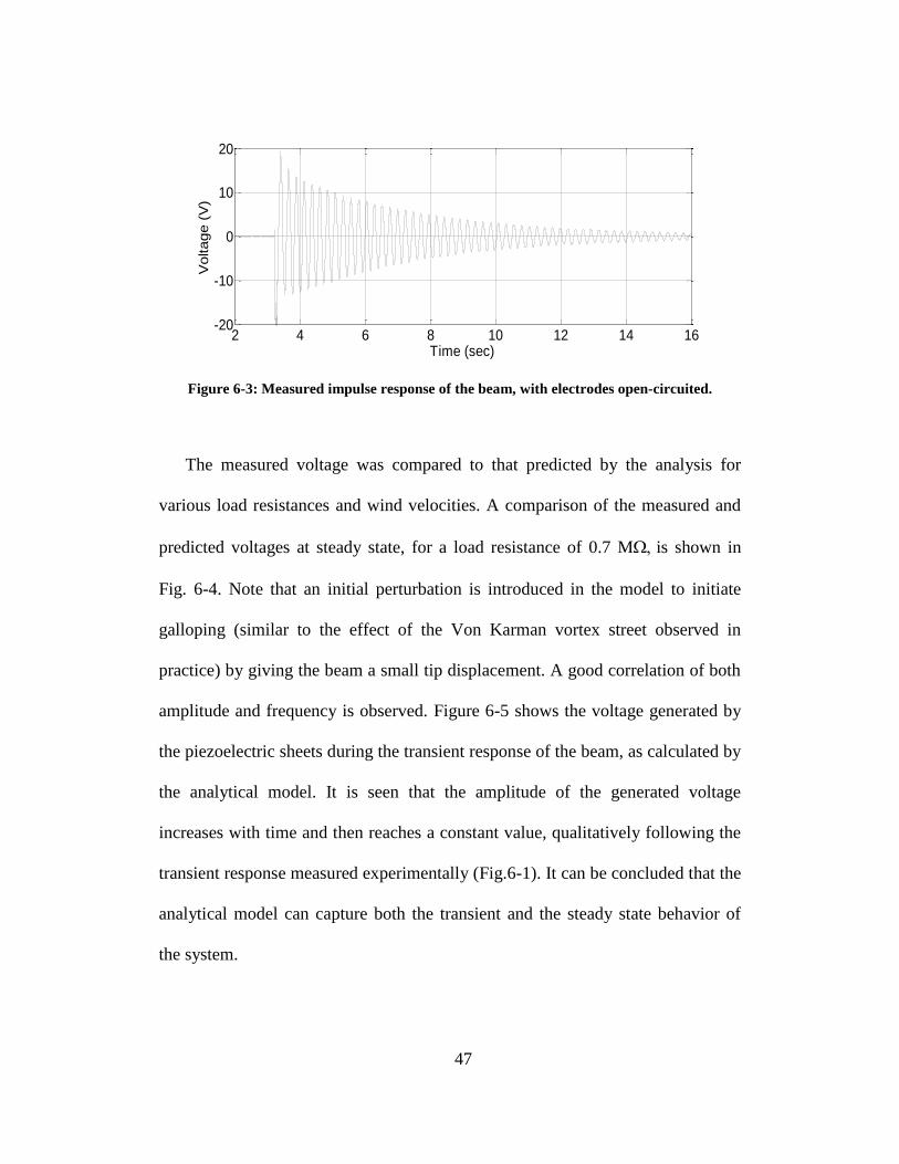
The mechanical damping ratio of the cantilever beam is calculated from the

impulse response of the beam. The voltage generated by the piezoelectric sheets,

with open-circuited electrodes, in response to a tip impulse is shown in Fig.6-3.

From these data, the damping is calculated using the logarithmic decrement.

64 64.5 65 65.5 66 66.5 67-40

-30

-20

-10

0

10

20

30

40

Time (sec)

Vo

lta

ge

(V

)

47

Figure 6-3: Measured impulse response of the beam, with electrodes open-circuited.

The measured voltage was compared to that predicted by the analysis for

various load resistances and wind velocities. A comparison of the measured and

predicted voltages at steady state, for a load resistance of 0.7 Mis shown in

Fig. 6-4. Note that an initial perturbation is introduced in the model to initiate

galloping (similar to the effect of the Von Karman vortex street observed in

practice) by giving the beam a small tip displacement. A good correlation of both

amplitude and frequency is observed. Figure 6-5 shows the voltage generated by

the piezoelectric sheets during the transient response of the beam, as calculated by

the analytical model. It is seen that the amplitude of the generated voltage

increases with time and then reaches a constant value, qualitatively following the

transient response measured experimentally (Fig.6-1). It can be concluded that the

analytical model can capture both the transient and the steady state behavior of

the system.

2 4 6 8 10 12 14 16-20

-10

0

10

20

Time (sec)

Voltage (

V)

48

Figure 6-4: omparison of measured and predicted voltage at steady state, 0.7 MΩload

resistance at wind speed of 8 mph.

Figure 6-5: Transient response of the beam as predicted by analysis, at incident wind speed

of 8.6 mph, and 0.7 MΩ load resistance

Good correlation is also observed between the measured and predicted steady

state voltage amplitudes as a function of load resistance (Fig.6-6) and wind speed

(Fig.6-7). It is seen that the generated voltage increases approximately linearly

with the wind velocity for a given load resistance. Note that the voltage generated

20 20.5 21 21.5 22 22.5 23-30

-20

-10

0

10

20

30

Time (sec)

Voltage (

V)

Predicted

Measured

0 2 4 6 8 10 12 14 16-30

-20

-10

0

10

20

30

Time (sec)

Pre

dic

ted V

oltage (

V)

49

by the piezoelectric sheets was on the order of 30V, which implies that small

signal electrical characteristics are no longer applicable. This may account for the

discrepancies between the predictions and the measured data. Other sources of

error could include the effect of the finite thickness bond layer, and discrepancies

between the operating conditions (for example, Reynolds number) of the present

experimental setup and the experimental setup used for the published

aerodynamic coefficients. Although the generated voltage increases with load

resistance and wind velocity, the device generates maximum power when the load

resistance is optimal. This trend can be seen in Fig.6-8. The power plotted is the

average power, which is half of the peak power.

Figure 6-6: Comparison of measured and predicted steady state voltage, as a function of load

resistance, at wind speed of 8.5 mph

0

5

10

15

20

25

30

35

0 0.2 0.4 0.6 0.8 1 1.2

Pea

k V

olt

age

(Vo

lts)

Load resistance (M)

Measured

Predicted

50

Figure 6-7: Comparison of measured and predicted steady state voltage as a function of

incident wind velocity, for 0.7 MΩ load resistance

Figure 6-8: Measured power as a function of load resistance, at 8.5 mph wind speed

0

5

10

15

20

25

30

35

40

45

0 2 4 6 8 10 12

Pea

k V

olt

age

(Vo

lts)

Incident wind velocity (mph)

Measured

Predicted

0.0

0.1

0.2

0.3

0.4

0.5

0.6

0 0.2 0.4 0.6 0.8 1 1.2

Aver

age

Po

wer

Outp

ut

(mW

)

Load resistance (M)

51

The variation of measured power output on wind velocity is shown in Figure

6-9, along with analytical predictions. These values correspond to the maximum

power output, based on a load resistance of 0.7 M. It is seen that the power

output progressively increases with increasing wind velocity. The power output is

negligible below a wind velocity of 5.6 mph due to the inherent structural

damping in the device. However, annual average wind speed estimates, for

example, in region of Texas is around 13 mph [37] , which implies that the range

of power output shown Fig.6-9 is practically achievable. For the prototype

galloping device, a maximum power output of 1.14mW was achieved at 10.5

mph. Experimental results by Ajitsaria et al. [10] have indicated a maximum

power of 250μW produced by their bimorph PZT bender based on harvesting

structural vibrations. It can be concluded that it may be possible to harvest larger

amounts of power using galloping devices compared to devices based on

structural vibrations.

Figure 6-9: Measured and predicted output power versus wind velocity, 0.7 MΩ load

resistance.

0.0

0.2

0.4

0.6

0.8

1.0

1.2

1.4

0 2 4 6 8 10 12

Aver

age

pow

er o

utp

ut

(mW

)

Incident wind velocity (mph)

Predicted

Measured

52

6.2 Galloping device (II): Triangular Section

An approach similar to D-section is used to measure experimental data for a

triangular section galloping device (II). The purpose of these experiments is to

verify the dynamic response from the model with measured tip displacement

response. Figure 6-10 shows a general accelerometer signal measuring in X and Y

direction. The accelerometer is attached to the tip of the beam as shown in Fig. 5-

2. Subjected to a constant incident wind speed in the wind tunnel, the signal

measured starts from rest, captures the transient response and settles at steady

state amplitude. As the angle of attack just goes out of the unstable region of

negative Cl slope, the response attains steady state amplitude. In order to continue

extracting energy from the galloping device, it is essential that the galloping

operation continues to be within the unstable region. Since there is no

piezoelectric material attached to the beam, no energy is being extracted.

53

Figure 6-10: Accelerometer voltage signal measuring X (blue line) and Y (green line)

acceleration at the tip of the beam, at incident wind speed of 7 mph

0 2 4 6 8 10 12-2

-1.5

-1

-0.5

0

0.5

1

1.5

2

time (sec)

Voltage (

V)

(repre

senting X

and Y

accele

ration)

sensitivity: 0.420V/g = 0.0428 V/(m/s2)

54

Figure 6-11: Transient tip displacement response (measured) of galloping device (II)

subjected to incident wind speed of 6.4 mph

The accelerometer signal is converted from voltage to acceleration using the

sensitivity factor. The acceleration is integrated over time twice to obtain a

displacement response of the beam tip. Figure 6-11 shows an integrated signal

representing transient response of tip displacement of the galloping beam at 6.4

mph wind speed. Figure 6-12 shows a close look at a steady state measured

response at same wind speed. The frequency of oscillation is determined

experimentally from the steady state and is found to be 6.5 Hz.

5 6 7 8 9 10 11 12

-20

-15

-10

-5

0

5

10

15

20

time (sec)

x a

nd y

dis

p (

mm

)

55

Figure 6-12: Steady state tip displacement response (measured) of galloping device (II)

subjected to incident wind speed of 6.4 mph

Table 6-1: Results for galloping device (II)

Measured Simulated

Wind Natural Stiffness Max. Beam Max. Beam

Speed frequency of the system tip deflection tip deflection

(mph) (Hz) (N/mm) (mm) (mm)

6.4 6.5 0.088 31.8 29

7.0 6.5 0.088 32.5 30.5

10.0 11.25 0.260 41 38

11.0 11.25 0.260 43 40.4

The simulated results for steady tip displacement are close to the measured

results. They follow a same increasing trend. Increasing wind speed result in an

increase in tip deflection, denoting higher strain energy produced in the beam.

Measurements are taken for two natural frequencies of the system, by changing

0 0.5 1 1.5 2 2.5 3-20

-15

-10

-5

0

5

10

15

20

time t (sec)

tip d

ispla

cem

ent

(mm

)

56

the beam length (L1, L2: see Table 5-3) and keeping the tip mass constant. In both

cases, the beam oscillations are noted to be at the natural frequency, that is, at

resonance. To initiate galloping, a higher minimum speed (7.5mph) is required for

the system with natural frequency = 11.25 Hz. For the system with lower natural

frequency, the corresponding minimum wind speed required is 5 mph. It shows

systems with very high natural frequencies may not be suitable for the galloping

device.

57

7. Summary and Conclusion

A device based on galloping piezoelectric cantilever beam was developed to

extract power from wind. The beam has a rigid tip body of D-shaped cross

section. The tip body undergoes galloping oscillations when subjected to incident

wind. Piezoelectric sheets bonded on the beam convert strain energy into

electrical energy.

The electrical power generated by a prototype device 325 mm long was

measured over a range of wind velocities, and the feasibility of wind energy

harvesting using this device was demonstrated. The power output was observed to

increase rapidly with increasing wind speed. Due to the structural damping of the

beam, a minimum wind velocity of 5.6 mph was required to generate power from

this device. For a wind velocity of 10.5 mph, a maximum power output of

1.14mW was measured.

An analytical model was developed including the aerodynamic properties of

the tip body, structural properties of the beam and the electro-mechanical

coupling of the piezoelectric sheets. Based on incident wind velocity, geometry

and other structural parameters of the galloping device, the model could predict

the dynamic voltage generated across load resistor, current produced and power

output. The model showed good correlation with measured data, and was able to

predict both the transient and the steady-state behavior of the device. It was

observed that beam geometry and mass parameters, which determine the natural

58

frequency of the system, play a significant role in the maximum power generated.

All these parameters can be optimized within the model to maximise the power

output.

Any tip body could be modeled by inputting appropriate sectional

aerodynamic data. Based on this data, dynamic angle of attack and aerodynamic

forcing on the device was predicted by the model, which in turn predicts power

output. In this way, a tip body with optimum aerodynamic properties can be

designed to maximize the power output of this device.

A 2nd

device based on galloping cantilever beam was developed and tested for

workability. The beam of this device has a rigid tip body of equilateral triangular

section. A study of the geometry of the tip body was carried out and the

equilateral triangle cross-section was observed to be more favourable to cause

galloping than other isosceles triangle cross-sections. Aerodynamic data for this

geometry was used in the analytical model to predict beam tip response. The

predicted result agreed with experimental measurements of beam tip response.

Galloping experiment was conducted for two different natural frequencies of the

system. Higher natural frequency of the system led to increasing the minimum

wind speed required to initiate galloping. This result was in conjunction with the

model.

A potential application of power generation using this device is to power

wireless sensor devices in large civil structures, exposed to natural wind. It can be

concluded that it is possible to harvest significantly more power using this kind of

59

device compared to a device based on ambient structural vibrations. The device

described in this paper forms a baseline for future advancements in development

of wind energy based piezoelectric power generators.

60

8. References

[1] Den Hartog, J.P., 1956, ―Mechanical Vibrations‖, Dover Publications Inc.,

New York, pp. 299-305.

[2] Chabart, O. and Lilien, J. L., 1998, ―Galloping of electrical lines in wind

tunnel facilities‖, Journal of Wind Engineering and Industrial Aerodynamics, Vol

74-76, pp. 967-976.

[3] Alonso, G., Meseguer, J. and Pérez-Grande, I., 2007, ―Galloping stability

of triangular cross-sectional bodies: A systematic approach,‖ Journal of Wind

Engineering and Industrial Aerodynamics 95, pp. 928–940.

[4] Kazakevich, M. I. and Vasilenko, A. G., 1996, ―Closed analytical solution

for galloping aeroelastic self-oscillations,‖ Journal of Wind Engineering and

Industrial Aerodynamics, 65, pp. 353-360.

[5] Laneville, A., Gartshore, I. S. and Parkinson, G. V., 1977, ―An

explanation of some effects of turbulence on bluff bodies‖ Proceedings of the

Fourth International Conference on Wind Effects on Buildings and Structures,

Cambridge University Press, pp. 333–341.

[6] Sodano, H., Park, G. and Inman D., 2004, ―Estimation of electric charge

output for piezoelectric energy harvesting‖, Strain, 40 (2), pp. 49-58.

[7] Umeda M., Nakamura K. and Ueha S., 1996, ―Analysis of the

transformation of mechanical impact energy to electric energy using piezoelectric

vibrator,‖ Japan. J. Appl. Phys. 35, pp. 3267–73.

[8] Roundy S., Wright P. K. and Rabaey J. M., 2004, ―Energy Scavenging for

wireless sensor networks with special focus on vibrations,‖ Kluwer Academic

Publishers.

[9] Ottman G. K., Hofmann H. F. and Lesieutre G. A., 2003, ―Optimized

Piezoelectric Energy Harvesting Circuit Using Step-Down Converter in

Discontinuous Conduction Mode,‖ IEEE Trans. Power Electronics, 18(2), pp.

696–703.

61

[10] Ajitsaria J., Choe S. Y., Shen D. and Kim D. J., ―Modeling and analysis of

a bimorph piezoelectric cantilever beam for voltage generation,‖ 2007, Smart

Materials and Structures, 16, pp. 447-454.

[11] Holst Centre, High Tech Campus 31, 5656 AE Eindhoven, Netherlands.

<www.holstcentre.com>

[12] AdaptivEnergy, 1000 Lucas Way Suite B, Hampton VA 23666, USA.

<www.adaptivenergy.com>

[13] Advanced Cerametrics, Inc., P.O. Box 128, 245 N. Main St., Lambertville,

NJ 08530, USA. <www.advancedcerametrics.com/pages/energy_harvesting>

[14] Mide Technology Corporation, 200 Boston Avenue, Suite 1000, Medford,

MA 02155, USA. <www.mide.com/products/volture/volture_catalog.php>

[15] PMG Perpetuum Ltd., Epsilon House, Southampton Science Park,

Southampton, SO16 7NS. 5. www.perpetuum.co.uk

[16] Jung, H.J., Lee, S.W. and Jang, D.D., 2009, ―Feasibility Studies on a New

Energy Harvesting Electromagnetic Device Using Aerodynamic Instability‖,

IEEE Transactions on Magnetics, 45(10), pp. 4376-4379.

[17] Wang D.A. and Ko H.H., 2010, ―Piezoelectric energy harvesting from

flow-induced vibration‖, Journal of Micromechanics and Microengineering,

20(2).

[18] Barrero-Gil A., Alonso G. and Sanz-Andres A., 2010 ―Energy harvesting

from transverse galloping‖, Journal of Sound and Vibration, 329(14), pp. 2873-

2883.

[19] Robbins, W. P., Morris, D., Marusic, I. and Novak, T. O., 2006, ―Wind-

Generated Electrical Energy Using Flexible Piezoelectric Materials‖,

IMECE2006-14050, ASME Publications-AD, Vol. 71, pp. 581—590.

[20] Humdinger Wind Energy <www.humdingerwind.com>

[21] Estrin D., Govindan R., and Heidemann J., (Eds.), 2000, ―Special Issue on

Embedding the Internet. Communications of the ACM‖, 43(5).

62

[22] Badrinath B. R., Srivastava M., Mills K., Scholtz J. and Sollins K., (Eds.),

2000, Special Issue on Smart Spaces and Environments IEEE Personal

Communications.

[23] Wang Y., Kenneth J. Loh, Lynch J. P., Fraser M., Kincho Law and Ahmed

Elgamal, 2006, ―Vibration Monitoring of the Voigt Bridge using Wired and

Wireless Monitoring Systems,‖ The Proceeding of 4th China-Japan-US

Symposium on Structural Control and Monitoring‘.

[24] Mainwaring A., Polastre J., Szewczyk R., Culler D. and Anderson, J.,

2002, ―Wireless sensor networks for habitat monitoring,‖ Proceedings of the 1st

ACM international workshop on Wireless sensor networks and applications,

Atlanta, Georgia, USA, pp. 88-97.

[25] Crossbow Technology Inc., 1421 McCarthy Boulevard, Milpitas CA

95035

[26] Evans, R. and Bergman, J., 2007, ―Relationships between cropping

sequences and irrigation frequency under self – propelled irrigation systems in the

northern great plains,‖ USDA annual report, Project number: 5436-13210-003-02.

[27] Jennifer Yick, Biswanath Mukherjee and Dipak Ghosal, 2008, ―Wireless

sensor network survey,‖ Computer Networks 52, 2292-2330.

[28] Ratkowski J., 1961, ―Experiments with galloping spans,‖ AIEE Winter

General Meeting New York, N.Y., paper 62.

[29] Alonso, G., Meseguer, J. and Pérez-Grande, I., 2005, ―Galloping

instabilities of two-dimensional triangular cross-section bodies‖, Experiments in

Fluids, 38, pp. 789-795.

[30] Alonso, G. and Meseguer, J., 2006, ―A parametric study of galloping of

two dimensional triangular cross section bodies‖, Journal of Wind engineering

and Industrial Aerodynamics, 94, pp. 241-253.

[31] Lee, P C Y., 1991, ―A Variational Principle for the Equations of

Piezoelectromagnetism in Elastic Dielectric Crystals‖, Journal of Applied

Physics, 69(11), pp. 7470.

[32] Nisse, E P E., 1967, ―Variational Method for Electroelastic Vibration

Analysis‖, IEEE Transactions on Sonics and Ultrasonics, Vol. SU-14(4), pp. 153.

63

[33] IEEE Standard on Piezoelectricity, ANSI/IEEE, Std. 176, 1987.

[34] Matlab Simulink, Mathworks.

[35] Product Information, 2010, Piezo Systems Inc., 65 Tower Office Park,

Woburn, MA 01801, USA. http://www.piezo.com/prodsheet2sq5H.html

[36] Analog devices, USA. http://www.analog.com/en/sensors/inertial-

sensors/adxl322/products/product.html

[37] Schwartz, M. N., and Elliot, D. L., 1993, ―United States Areal Wind

Resource Assessment‖, Report PNL-SA-21606, Presented at the Alternate Fuels

and the Environment Symposium, Denver, CO.

64

VITA

Rohan Ram Mahadik was born in Ratnagiri, India. After completing his study

in schools at Mumbai and Ahmedabad, India, he entered Nirma University in

Ahmedabad, India. He received the degree of Bachelor of Technology in

Mechanical Engineering from Nirma University in June, 2007. During the

following year, he was employed as Member, Research and Development,

Chassis-Suspension, at TVS Motor Company in Bangalore, India. In September,

2008, he entered the Graduate School in Aerospace engineering at the University

of Texas at Austin.

Permanent email: rohanez@gmail.com

Permanent Address: 203 Kirtankunj, Champaner Society,

Usmanpura, Ashram Road,

Ahmedabad-380013

India

This thesis was typed by the author.