solar plant startup optimization - indian institute of...

Solar Plant Startup

Optimization

Predictive controller

to optimize the start-

up cost in Solar

Power Plants.

Presentation by: Prabir Purkayastha

Co-Authors: K.V. Lakshmi, V. Agrawal, R. Talwar

Overview

INTRODUCTION

OPTIMISATION OF OPERATION OF CSP WITH TES

FIRST PRINCIPLES MODELING OF CSP WITH TES

DYNAMIC SIMULATOR OVERVIEW

SOLAR PLANT START UP OPTIMIZATION

CONVENTIONAL PLANT STARTUP OPTIMIZATION

REFERENCES

Operating Environment

Freitag, 27. Dezember

2013

Fußzeilentext 3

Why Optimise the operation of a CSP?

• To decide when to switch the turbine on (or off)

• To decide when to draw heat from storage and supply to the

power block

• To adapt to a time-of-day tariff regime

These are binary choices that are required to be made at all

times during the chosen operating horizon – an 8-hour shift or a

24-hour day or a week

Modeling Approach


2013

Fußzeilentext 4

The very nature of these operational decisions calls for an

approach that can deal with integer and real variables that

represent the operating choices in discrete time blocks of

15 or 60 minutes’ duration

The decision problem can be modeled adequately by

means of a mixed integer linear programming (MILP)

model

Model Framework


2013

Fußzeilentext 5

Objective

Maximise the net margin between the tariff earning from

net power despatched and the following costs

•Start-up cost

•O&M cost

Constraints

A number of constraints are required to capture adequately

the techno-economics of a CSP plant with thermal storage

Modeling Approach


2013

Fußzeilentext 6

The major data requirements are

•Hourly solar insolation

•Plant capacity

•Solar field

•Thermal energy storage

•Power block

•Performance curves

These are obtained from STEAG’s in-house first-

principles model for CSP with TES (presented after the

modeling approach).

Model Framework


2013

Fußzeilentext 7

Decision Variables

The following non-negative variables are relevant to the problem. The time

block is denoted by the index T.

X(T) a binary variable denoting whether the power block is running in T

GROSSE(T) gross generation in T

NETE(T) net generation in T

STORE(T) stored energy at start of T

INSOLE(T) energy captured by solar block in T

INSOLES(T) portion of energy captured by solar block sent to storage

INSOLEP(T) portion of energy from solar block sent directly to power block

USTORE(T) stored energy used in T

STARTE(T) energy used for power block start-up in T

Model Framework


2013

Fußzeilentext 8

Constraints

A number of constraints are required to capture adequately

the techno-economics of a CSP plant with thermal storage.(In the following constraints f and g denote functions

a. Energy captured by solar block depends on the

insolation. The latter data will be an input to the model.

INSOLE(T) = f(insolation_data)

Model Framework


2013

Fußzeilentext 9

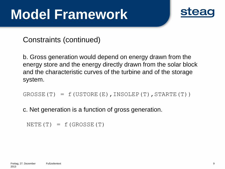
Constraints (continued)

b. Gross generation would depend on energy drawn from the

energy store and the energy directly drawn from the solar block

and the characteristic curves of the turbine and of the storage

system.

GROSSE(T) = f(USTORE(E),INSOLEP(T),STARTE(T))

c. Net generation is a function of gross generation.

NETE(T) = f(GROSSE(T)

Model Framework


2013

Fußzeilentext 10


d. Gross generation would be limited to a given capacity and

whether the unit is available in the time block or not.

GROSSE(T) <= captg*X(T)

e. Inter-temporal changes in the gross generation would be

limited by the given ramp rates applied to gross generation in the

preceding time block.

f(GROSSE(T-1)) <= GROSSE(T) <= g(GROSSE(T-1)))

Model Framework


2013

Fußzeilentext 11


f. Energy balances and limits on energy that can be drawn from storage.

INSOLE(T) = INSOLES(T) + INSOLEP(T)

STORE(T+1) = STORE(T) + INSOLES(T) – USTORE(T) – STARTE(T)

f(USTORE(T-1)) <= USTORE(T) <= g(USTORE(T-1))

g. Initial conditions at start of first time block T1.

X(T1) = x1

STORE(T1) = store1

Ebsilon Model- 1st Principle

Thermodynamic Modeling


2013

Fußzeilentext 12

The Solar-Thermal plant behavior can be examined using the Ebsilon

tool

INTRODUCTION: Solar Plant

Start-Up Time Optimization

Optimal Start-up strategies vary with theType and Construction of the Solar Plant:

HTF Based/DSG based

With or without Storage

With or without backup Boiler.

Start-Up time computed using predictivecontroller

Validate using dynamic Solar Simulator Reduction in Start Up time

Additional Revenue

Start-up procedure realized at any specificday depends on :

Irradiation profile1. Time of the day2. The season.

Thermal State of HTF in the morningi.e. Initial Condition

1. Number of night hours2. Night-time ambient temperature3. Storage usage during the night

Other meteorological conditions likewind speed, presence of clouds etc.

Reduction in Start Up time

Additional Revenue

INTRODUCTION: Solar Plant

Start-Up Time Optimization


2013

Fußzeilentext 15

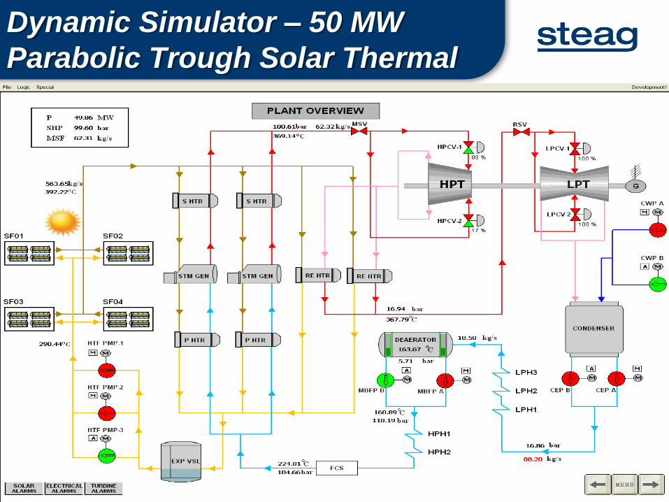
Dynamic Simulator – 50 MW

Parabolic Trough Solar Thermal


Parabolic Trough Features:

Indirect steam generation - HTF Based.

Solar Field : 1. Total 112 Loops; 2. Four solar subfields having 28 loops each; 3. Collector operation Modes: Solar Tracking; 4. Complete defocus & specific

position; 5. Control for HTF Outlet Temperature.

Solar Steam Generation : 1. Three HTF Pumps, 2.Two streams of solar super heaters, steam generator and a preheater; 3. Two streams of reheaters; 4.Steam generator level control.

Turbine : 1.Turbine with HP and LP Stage; 2.Single reheat and Governing Controls.

Condensate and Feedwater System: Two MDBFPs, Three LP and Two HP heaters.

PROCESS

+

CONTROL

MODELS

(In TRAX)

SHARED

MEMORY

HUMAN

MACHINE

INTERFACE

(In INTOUCH)

,

Solar Plant Start-Up Time Possible

Optimization Options :

Options for Start Up time Reduction

3. Better Design for

Maximum Heat Capture

and Minimum Loss

5. Optimizing

inlet temperature

and amount of

HTF to solar

heat exchangers

1. Quick Heating of

HTF/Steam(using

thermal storage)

4. Better

Control

System

2. Quick Heating of

HTF/Steam (using quick

start backup boiler)

Solar Plant Start-Up Time Optimization -

Formulation

Objective Function is defined to minimize the start up time:

where, x[n] are the state variables, u[n] are the control variables, and

are the optimizing weights corresponding to state and control variables, N is the

prediction time horizon

For Nonlinear Plant, Partial Differential Model Equations:

Subjected to Constraint Equations:

Here, constraint are Thermal Stresses on heat exchangers walls,

-σ < Differential Metal-wall Temperatures < +σ

Optimized Set Points:

a. Flow of HTF to Heat Exchangers

b. Temperature at which HTF to be passed to Heat Exchangers

c. Heat flow from Storage/Backup Boiler (if present).

Functional Block Diagram

PROCESS

VARIABLES FROM

SOLAR SIMULATOR

SOLAR HEAT EXCHANGERS

MODELLING: Preheater,

Steam Generator,Economizer

Iteration

SQP

OPTIMIZER

Cost Function = Min. start-up time

Constraint: Thermal Stresses

OPTIMIZATION GOALS

OPTIMIZED

VARIABLES:

Main Steam FlowDrum PressureMetal and Steam Temperatures

OPTIMIZED

SET POINTS

INPUTS:

Predicted DNIWind SpeedHTF Amount HTF TemperatureHeat from Storage/Backup Boiler

NON-LINEAR MODEL PREDICTIVE CONTROLLER


2013

Fußzeilentext 20


Parabolic Trough Solar HTF Path


2013

Fußzeilentext 21

Dynamic Simulator : Parabolic

Trough Heat Exchanger Path

Nonlinear Model Predictive Controller (NMPC) to minimize thestart-up time for Subcritical Suratgarh 250MW Thermal Power Plant.

Constraints:

1. Fuel Cost

2. Thermal stresses on critical walls of Heat Exchangers.

Heat Exchangers are modeled in Modelica Language usingOpenModelica Compiler, as the simulation environment.

1.Highly Non Linear Solver available2.Multi-variable, Time Based Partial Differential Equations3.Component Based Modeling, using connectors4.An Open Source & commercial versions available, Dymola etc.5.Supports huge Multi-Domain Modelica Standard Library6.External linking with Non-Modelica Environments

Conventional Boiler Startup

Optimization

Optimization Technique: Sequential Quadratic Programming.

Optimizer computes the following optimal set-points:

1. Heat input

2. Control valve opening position of HP by-pass station.

Objective Function is defined to match the desired pressureprofile, for 2 to 60 bar drum pressure:

where, = tuning weights= pressure at each time step

Results:

Start-up time, between 2 to 60bar drum pressure:

Actual Start-up Time: 4 to 6 Hours

With Predictive Controls : Reduction of 30 – 45 mins.


Optimization


Optimization- Block Diagram

REAL BOILER /

SIMULATOR MODEL

BOILER

MODEL

(OpenModelica

Platform)

Iteration

SQP

OPTIMIZER

Cost function

= minimum

OPTIMIZATION GOALS

Optimized

Variables

Optimized

Set points

Inputs

Process

Inputs &

Variables

References

K. Azizian, M. Yaghoubi, I. Niknia, and P. Kanan, “Analysis of

Shiraz Solar Thermal Power Plant Response Time”, in Journal of

Clean Energy Technologies, Vol. 1, No. 1, January 2013.

Juergen H. Peterseim, Udo Hellwig, Manoj Guthikonda, and Paul

Widera, “Quick Start-up Auxiliary Boiler / Heater – Optimizing

Solar Thermal Performance”, in SolarPACES 2012 conference

Marrakech, 11-14 September 2012.

Tobias Hirsch, Heiko Schenk, Norbert Schmidt and Richard

Meyer‚ “Dynamics Of Oil-based Parabolic Trough Plants - Impact

Of Transient Behaviour On Energy Yields”, Proc. of the 2010

SolarPACES conference, Perpignan, France (2010).

Modelica home page: www.openmodelica.org

References

Hubert Thieriot, Maroun Nemer, Mohsen Torabzadeh-Tari, Peter

Fritzson, Rajiv Singh, “Towards Design Optimization with

OpenModelica including Parameter Optimization with Genetic

Algorithms ”, in 8th International Modelica Conference, 2011.

Rüdiger Franke, and Bernd Weidmann, “Startup optimization for

steam boilers in E.ON power plants”, in ABB Review 1/2008.

R¨udiger Franke, B.S. Babji, Marc Antoine and Alf Isaksson‚

“Model-based online applications in the ABB Dynamic

Optimization framework”, in Modelica Association 2008, March

3rd - 4th ,

THANK YOU

REFERENCE SLIDES

1. NMPC CONTROLLER

2. OPEN MODELICA FEATURES

3. CONVENSIONAL SIMPLE BOILER MODEL

4. CONVENSIONAL SIMPLE BOILER EQUATIONS

Receding horizon philosophy

A multivariable control algorithm that uses:

an internal dynamic model of the nonlinear process.

a history of past control moves

an optimization cost function, P over the receding

prediction horizon.

Steps:

At time t: solve an optimal control problem over a

finite future horizon of N steps.

Only apply the first optimal move.

At time t+1: Get the new measurements, repeat the

optimization.

Advantage of repeated on-line optimization:

FEEDBACK

It will sample the current plant state and

computes/predicts a cost minimal control strategy for

relatively short time horizon in the future.

,

1.Conventional Boiler Startup Optimization-

Non-linear Model Predictive(NMPC) Controller

,

Object-oriented Modeling Paradigm.

Declarative type equation based textual language.

Multivariable Time Based Differential Equation for simulation purposes.

Component Based Modeling: using connectors that reduces modeling errors.

Multi-Domain Hybrid Modeling that supports Modelica Standard Library (containsabout 1280 model components and 910 functions, from different physical domainslike electrical, mechanical, hydraulic domains, etc.).

External linking of Library Functions developed in Non-Modelica Languages can beinterlinked, like steam tables defined in Fortran Compiler.

Modelica Simulation Environments are available as open source and alsocommercially, like CATIA Systems, CyModelica, Dymola, LMS AMESim,JModelica.org, MapleSim, SCICOS, SimulationX, Vertex and Wolfram SystemModeler.

Reference: www.openmodelica.org

2. Conventional Boiler Startup Optimization-

OpenModelica Platform


Component Based Boiler Model

Metal and Steam Temperatures

FURNACE

BOILER DRUM

SUPERHEATERS1. LTSH2. SHDP3. SHPL

ECONOMIZER

REHEATER

Fuel Flow Main Steam Flow

Drum PressureHPBP VLV POSITION

Thermal Stresses

INPUTSCOMPONENTSIn MODELICA OUTPUTS

TUNING PARAMETERS: Heat Transfer CoefficientsThermal and Flow ConductanceEmissivity Constants


OpenModelica Platform

The Simple Boiler Drum Equations :

Steam temperature is a non-linear function of pressure inside drum,

Feedwater flow is equal to the main steam flow, assuming no blowdown .

Steam temperature inside drum is assumed to be equal to the metal wall temperature.

Energy transferred from flue gas to riser water walls Q, is a function of the difference between flue gas temperature and metal temperature.

where,

Heat given to boiler drum Q, is also equal to the energy stored in the water walls and the heat given to the steam. Where,

HPBP control linear valve equation:

solar plant startup optimization - indian institute of...

Documents