solar disinfection for point of use water …haiti is the poorest nation in the western hemisphere...
TRANSCRIPT

SOLAR DISINFECTION FOR POINT OF USE WATER TREATMENT IN HAITI
by
Peter M. Oates
Submitted to the Department of Civil and Environmental Engineering on May 11th, 2001 in partial fulfillment of the requirements for the degree of Master of Engineering in Civil and Environmental Engineering. ABSTRACT Haiti is the poorest nation in the western hemisphere and cannot afford conventional means of water treatment. Consequently, waterborne disease causes great suffering and death throughout the Haitian community. This research effort investigates using solar disinfection or SODIS for point-of-use water treatment in Haiti, which can provide disease-free water at the cost of a plastic bottle. The SODIS treatment process consists of filling plastic bottles with water and exposing them to sunlight. SODIS operates on the principle that sunlight-induced DNA alteration, photo-oxidative destruction, and thermal effects will inactivate microorganisms. To achieve adequate disinfection, an area should receive at least 500 W/m2 of radiation for 5 hours. Haiti and other developing countries do not have sufficient meteorological data to assess if they meet this threshold. A mathematical model is presented, calibrated, and used to simulate monthly average, minimum, and maximum daily sunlight intensity profiles to estimate if Haiti would be suitable for SODIS. This method is general in that it can be used to simulate sunshine intensity profiles anywhere in the world per degree longitude and latitude. The sunshine simulations suggest that SODIS would be applicable throughout Haiti year-round. Field studies were conducted in Haiti during January 2001 to test SODIS. SODIS efficacy was evaluated by the inactivation of total coliform, E. coli, and H2S-producing bacteria under different natural conditions. Exposure period proved critical. Under various sunshine intensities, bottle water temperatures, and initial bacterial amounts, 1-day exposure achieved complete bacterial inactivation 52 % of the time, while the 2-day exposure period achieved 100 % microbial inactivation for every test. To maintain the beauty of this technology, a practical way of providing people with cold water every morning that has undergone a 2-day exposure period has been developed and termed a “SODIS triangle.” Essentially, it consists of three groups of bottles that are rotated every morning, so two groups are out in the sun and one is being used for consumption. It is hoped that this relatively new disinfection method will provide an economically feasible technology to improve water quality and public health in Haiti. Thesis Supervisors: Peter Shanahan and Martin Polz Title: Lecturer and Assistant Professor

3
DEDICATED TO MY PARENTS PETER AND NANCY TO WHOM I OWE EVERYTHING
TO MY SISTER KATE FOR NOT LETTING ME BE COMPLETELY ENGULFED BY SCIENCE
TO WLBC AND THE LATE NIGHTS OF PHILOSPHY THAT HELPED PUT ME HERE
A HEARTFELT THANK YOU TO MY TEAMATES AND FRIENDS NADINE, DANIELE, AND FARZANA
AND MY ADVISORS PETER SHANAHAN AND MARTIN POLZ
A MOST SINCERE THANK YOU TO THOSE WHO MADE THIS EXPERIENCE POSSIBLE SUSAN MURCOTT; PHIL, BILL, TRUDI, AND KEVIN FROM GIFT OF
WATER; AND NATHAN AND WANDA FOR THEIR HOSPITATLIY

4
TABLE OF CONTENTS
SECTION I: OVERVIEW OF DRINKING WATER IN HAITI .............................. 10
1 INTRODUCTION................................................................................................... 11 1.1 HAITIAN WATER RESOURCES ............................................................................ 13
1.1.1 Precipitation ............................................................................................. 13 1.1.2 Rivers and Surface Water ......................................................................... 14 1.1.3 Groundwater ............................................................................................. 15 1.1.4 Impacts of Deforestation........................................................................... 16
1.2 HAITIAN WATER SUPPLY................................................................................... 18 1.3 HAITIAN WATER QUALITY ................................................................................ 21 1.4 POINT-OF-USE WATER TREATMENT .................................................................. 24
SECTION II: SODIS FOR POINT OF USE WATER ............................................... 27
TREATMENT................................................................................................................. 27
2 SODIS: SOLAR WATER DISINFECTION........................................................ 28 2.1 SODIS INTRODUCTION AND DEVELOPMENT ..................................................... 28 2.2 SOLAR RADIATION AND DISINFECTION.............................................................. 29 2.3 DNA ALTERATION BY UV................................................................................. 30 2.4 PHOTO-OXIDATIVE DISINFECTION..................................................................... 32 2.5 THERMAL INACTIVATION................................................................................... 35 2.6 INACTIVATION OF INDICATOR ORGANISMS AND PATHOGENS ............................ 37
2.6.1 Indicator Organisms ................................................................................. 37 2.6.1.1 Total Coliform ...................................................................................... 38 2.6.1.2 Fecal Coliform and E. coli .................................................................... 39
2.6.2 Inactivation of Specific Microorganisms and Heat Sensitivity................. 40 2.7 UV-ENHANCED BACTERIAL GROWTH AND BACTERIAL REGROWTH ................. 42
3 IMPORTANT SODIS VARIABLES .................................................................... 45 3.1 HAITIAN CLIMATE ............................................................................................. 45
3.1.1 Haitian Sunshine....................................................................................... 46 3.1.2 Mathematical Development of Sunshine Simulation ................................ 49 3.1.3 Simulation of Haitian Sunshine ................................................................ 55 3.1.4 Haitian Temperature................................................................................. 64 3.1.5 Haitian Topography.................................................................................. 65
3.2 TURBIDITY......................................................................................................... 68 3.3 SODIS BOTTLE CHARACTERISTICS ................................................................... 69
3.3.1 PET Bottles ............................................................................................... 69 3.3.2 Water Depth .............................................................................................. 69 3.3.3 Transmittance Loss and Household Preference ....................................... 70
3.4 ECONOMIC CONSIDERATIONS ............................................................................ 71 3.5 ACCEPTANCE OF SODIS.................................................................................... 72

5
SECTION III: MATERIALS AND METHODS ......................................................... 74
4 FIELD TESTS......................................................................................................... 75 4.1 SUNLIGHT INTENSITY......................................................................................... 75 4.2 TEMPERATURE ................................................................................................... 76 4.3 TURBIDITY......................................................................................................... 76 4.4 MICROBIAL PRESENCE ABSENCE TESTS ............................................................ 77
4.4.1 Total Coliform and E. coli ........................................................................ 77 4.4.2 HACH PathoScreenTM .............................................................................. 79
5 EXPERIMENTAL SETUP AND PROCEDURE................................................ 81 5.1 EXPERIMENTAL SETUP....................................................................................... 81 5.2 EXPERIMENTAL PROCEDURE.............................................................................. 82
SECTION IV: RESULTS AND DISCUSSION ........................................................... 85
6 DAILY RESULTS AND DISCUSSION ............................................................... 86 6.1 RESULTS FOR WATER COLLECTED ON 01/12/01 ................................................ 86 6.2 RESULTS FOR WATER COLLECTED ON 01/13/01 ................................................ 89 6.3 RESULTS FOR WATER COLLECTED ON 01/15/01 ................................................ 92 6.4 RESULTS FOR WATER COLLECTED ON 01/16/01 ................................................ 94 6.5 RESULTS FOR WATER COLLECTED ON 01/17/01 ................................................ 95 6.6 RESULTS FOR WATER COLLECTED ON 01/18/01 ................................................ 99 6.7 RESULTS FOR WATER COLLECTED ON 01/19/01 .............................................. 103 6.8 RESULTS FOR WATER COLLECTED ON 01/20/01 .............................................. 105 6.9 RESULTS FOR 01/21/01 .................................................................................... 107
7 SUMMARY OF RESULTS AND DISCUSSION .............................................. 108 7.1 SUMMARY OF RESULTS.................................................................................... 109
7.1.1 Turbidity.................................................................................................. 109 7.1.2 Sunshine and Temperature ..................................................................... 109 7.1.3 Measured Intensity Comparison to Model Prediction............................ 111 7.1.4 Overall Microbial Analysis..................................................................... 113
7.2 DISCUSSION ..................................................................................................... 114
SECTION V: PRACTICAL APPLICATION GUIDELINES ................................. 118
8 PRACTICAL SODIS PROCEDURE ................................................................. 119 8.1 BOTTLES .......................................................................................................... 119 8.2 WATER ............................................................................................................ 120 8.3 EXPOSURE........................................................................................................ 121 8.4 ANTICIPATED MISTAKES.................................................................................. 123
SECTION VI: SUMMARY AND CONCLUSIONS ................................................. 124
9 SUMMARY AND CONCLUSIONS ................................................................... 125

6
APPENDIX: CODE USED FOR SUNLIGHT SIMULATION................................ 129
REFERENCES.............................................................................................................. 134

7
FIGURES AND TABLES
LIST OF FIGURES FIGURE 1-1. MAP OF HAITI............................................................................................................................ 12 FIGURE 2-1. SODIS OVERVIEW .................................................................................................................... 28 FIGURE 2-2. IMPORTANT COMPONENTS OF THE ELECTROMAGNETIC SPECTRUM (SOLOMON, 1996) ............. 29 FIGURE 2-3. UV-A AND TEMPERATURE EFFECT ON FECAL COLIFORM (EAWAG/SANDEC, TECHNICAL
NOTES). ............................................................................................................................................... 30 FIGURE 2-4. FORMATION OF THYMINE DIMERS (RAVEN AND JOHNSON, 1996; MATHEWS AND VAN HOLDE,
1996) ................................................................................................................................................... 31 FIGURE 2-5. AEROBIC VS. ANAEROBIC MICROBIAL INACTIVATION (REED, 1997)......................................... 34 FIGURE 2-6. SYNERGISTIC EFFECTS OF UV AND TEMPERATURE (EAWAG/SANDEC, TECHNICAL NOTES) 36 FIGURE 2-7. BACTERIAL REGROWTH (WEGELIN ET AL., 1994) ...................................................................... 43 FIGURE 3-1. DISCRETIZATION OF HAITI (NASA LANGLEY RESEARCH CENTER ATMOSPHERIC SCIENCES
DATA CENTER, 2001) .......................................................................................................................... 46 FIGURE 3-2. AVERAGE MONTHLY VALUE OF TOTAL DAILY RADIATION (NASA LANGLEY RESEARCH
CENTER ATMOSPHERIC SCIENCES DATA CENTER, 2001)..................................................................... 48 FIGURE 3-3. FOURIER SERIES OF SUNSHINE INTENSITY FOR 3 DAYS STARTING AND ENDING AT MIDNIGHT . 53 FIGURE 3-4. MODEL VALIDATION OF SIMULATED VERSUS OBSERVED SUNSHINE INTENSITY PROFILE......... 56 FIGURE 3-5. SIMULATED INTENSITY PROFILE FOR EACH MONTH IN AREA 1 (NASA LANGLEY RESEARCH
CENTER ATMOSPHERIC SCIENCES DATA CENTER, 2001)..................................................................... 57 FIGURE 3-6. COMPARISON OF SIMULATED TO OBSERVED AVERAGE PEAK THREE-HOUR AVERAGE
INTENSITIES (NASA LANGLEY RESEARCH CENTER ATMOSPHERIC SCIENCES DATA CENTER, 2001) . 58 FIGURE 3-7. YEARLY FIVE-HOUR AVERAGE INTENSITY PROFILE OF HAITI (NASA LANGLEY RESEARCH
CENTER ATMOSPHERIC SCIENCES DATA CENTER, 2001)..................................................................... 59 FIGURE 3-8. YEARLY FIVE-HOUR MINIMUM INTENSITY PROFILE OF HAITI (NASA LANGLEY RESEARCH
CENTER ATMOSPHERIC SCIENCES DATA CENTER, 2001)..................................................................... 60 FIGURE 3-9. AVERAGE PERCENT DAY TIME CLOUD COVER (NASA LANGLEY RESEARCH CENTER
ATMOSPHERIC SCIENCES DATA CENTER, 2001) .................................................................................. 61 FIGURE 3-10. YEARLY FIVE-HOUR MAXIMUM INTENSITY PROFILE OF HAITI (NASA LANGLEY RESEARCH
CENTER ATMOSPHERIC SCIENCES DATA CENTER, 2001)..................................................................... 62 FIGURE 3-11. YEARLY FIVE-HOUR AVERAGE, MAXIMUM, AND MINIMUM INTENSITY PROFILE OF HAITI
(NASA LANGLEY RESEARCH CENTER ATMOSPHERIC SCIENCES DATA CENTER, 2001) ..................... 63 FIGURE 3-12. AVERAGE TEMPERATURE PROFILE (NASA LANGLEY ATMOSPHERIC SCIENCES DATA CENTER,
2001) ................................................................................................................................................... 64 FIGURE 3-13. PHYSIOGRAPHICAL REGIONS OF HAITI (USAID, 1985) ........................................................... 66 FIGURE 3-14. HAITIAN TOPOGRAPHICAL MAP (GENERATED BY GEOVU, MATLAB, AND TECPLOT USING
NOAA DATA)...................................................................................................................................... 67 FIGURE 3-15. TURBIDITY ASSESSMENT (EAWAG/SANDEC, TECHNICAL NOTES)...................................... 68 FIGURE 4-1. KIPP AND ZONEN SOLRAD KIT................................................................................................... 75 FIGURE 4-2. HACH POCKET TURBIDIMETER ............................................................................................... 76 FIGURE 4-3. NEGATIVE (LEFT) AND POSITIVE (RIGHT) RESULTS OF TOTAL COLIFORM BCP TEST ................. 78 FIGURE 4-4. MUG (4-METHYLUMBELLIFERYL- β -DIBLUCUROMIDE) (MAIER ET AL., 2000)......................... 78 FIGURE 4-5. NEGATIVE (LEFT) AND POSITIVE (RIGHT) RESULTS OF E. COLI MUG TEST................................ 79 FIGURE 4-6. NEGATIVE (LEFT) AND POSITIVE (RIGHT) RESULTS OF H2S PATHOSCREENTM TEST................... 80 FIGURE 5-1. A TYPICAL ROOF TOP EXPERIMENT .......................................................................................... 83 FIGURE 6-1. WATER SOURCE FOR 01/12/01 .................................................................................................. 86 FIGURE 6-2. SUNLIGHT INTENSITY, AVERAGE SODIS BOTTLE TEMPERATURE, AND CORRESPONDING
DISINFECTION THRESHOLDS FOR 01/12/01 .......................................................................................... 87 FIGURE 6-3. ON-SITE WATER SOURCE FOR 01/13/01 ..................................................................................... 89 FIGURE 6-4. SUNLIGHT INTENSITY, AVERAGE SODIS BOTTLE TEMPERATURE, AND CORRESPONDING
DISINFECTION THRESHOLDS FOR 01/13/01 .......................................................................................... 90

8
FIGURE 6-5. SUNLIGHT INTENSITY, AVERAGE SODIS BOTTLE TEMPERATURE, AND CORRESPONDING DISINFECTION THRESHOLDS FOR 01/15/01 .......................................................................................... 92
FIGURE 6-6. SUNLIGHT INTENSITY, AVERAGE SODIS BOTTLE TEMPERATURE, AND CORRESPONDING DISINFECTION THRESHOLDS FOR 01/16/01 .......................................................................................... 94
FIGURE 6-7. "THE FESTERING PIT" WATER SOURCE FOR 01/17/01................................................................. 96 FIGURE 6-8. GIFT OF WATER FILTER............................................................................................................. 97 FIGURE 6-9. SUNLIGHT INTENSITY, AVERAGE SODIS BOTTLE TEMPERATURE, AND CORRESPONDING
DISINFECTION THRESHOLDS FOR 01/17/01 .......................................................................................... 98 FIGURE 6-10. LOCAL STREAM WATER SOURCE FOR 01/18/01...................................................................... 100 FIGURE 6-11. SUNLIGHT INTENSITY, AVERAGE SODIS BOTTLE TEMPERATURE, AND CORRESPONDING
DISINFECTION THRESHOLDS FOR 01/18/01 ........................................................................................ 101 FIGURE 6-12. SUNLIGHT INTENSITY, AVERAGE SODIS BOTTLE TEMPERATURE, AND CORRESPONDING
DISINFECTION THRESHOLDS FOR 01/19/01 ........................................................................................ 103 FIGURE 6-13. SUNLIGHT INTENSITY, AVERAGE SODIS BOTTLE TEMPERATURE, AND CORRESPONDING
DISINFECTION THRESHOLDS FOR 01/20/01 ........................................................................................ 105 FIGURE 6-14. SUNLIGHT INTENSITY, AVERAGE SODIS BOTTLE TEMPERATURE, AND CORRESPONDING
DISINFECTION THRESHOLDS FOR 01/21/01 ........................................................................................ 107 FIGURE 7-1. AVERAGE SUNLIGHT AND BOTTLE WATER TEMPERATURE OBSERVED IN HAITI DURING
JANUARY ........................................................................................................................................... 109 FIGURE 7-2. AVERAGE STORMY DAY PROFILE OBSERVED FOR THE 13TH AND 15TH OF JANUARY (2 OF 9 DAYS)
.......................................................................................................................................................... 110 FIGURE 7-3. AVERAGE NON-STORMY DAY PROFILE FOR PARTLY CLOUDY TO MOSTLY SUNNY DAYS (7 OF
9). ...................................................................................................................................................... 111 FIGURE 9-1. WATER IN THE HAITIAN COMMUNITY ..................................................................................... 127

9
LIST OF TABLES TABLE 1-1. PRINCIPAL CATCHMENT AREAS OF HAITI (LIBRARY OF CONGRESS, 1979) ................................ 14 TABLE 1-2. GROUNDWATER POTENTIALS FOR 22 SELECTED AREAS (HARZA, 1979)................................... 15 TABLE 1-3. DEFORESTATION AND RIVER DISCHARGES (OAS, 1972; HARZA, 1979; SHELADIA ASSOCIATES,
1983) ................................................................................................................................................... 17 TABLE 1-4. WATER SUPPLY SYSTEMS (HARZA, 1979; USAID, 1985) ........................................................ 20 TABLE 1-5. INFECTIOUS AGENTS PRESENT IN RAW DOMESTIC WASTEWATER (METCALF & EDDY, 1991)... 22 TABLE 1-6. SOME REPORTED CASES OF WATER RELATED DISEASES IN 1980 (CONADEPA, 1984)............ 23 TABLE 2-1. CRITERIA FOR AN IDEAL INDICATOR ORGANISM (MAIER ET AL., 2000) ...................................... 37 TABLE 2-2.VIRUS-COLIFORM RATIOS FOR SEWAGE AND POLLUTED SURFACE WATERS (MASTERS, 1997).. 38 TABLE 2-3. INDICATOR ORGANISMS USED IN ESTABLISHING PERFORMANCE CRITERIA FOR VARIOUS WATER
USE (METCALF AND EDDY, 1991) ....................................................................................................... 39 TABLE 2-4. SODIS INACTIVATION OF MICROORGANISMS ............................................................................ 40 TABLE 2-5. THERMAL DESTRUCTION OF MICROORGANISMS (FEACHEM ET AL., 1983).................................. 41 TABLE 3-1. RECOMMENDED AVERAGE DAY FOR EACH MONTH (DUFFIE AND BECKMAN, 1980).................... 50 TABLE 3-2. ADJUSTMENT FOR DAILY TIME (WUNDERLICH, 1972) ............................................................... 54 TABLE 3-3. AVERAGE MONTHLY TEMPERATURE RANGE °C FOR EACH AREA (NASA LANGLEY
ATMOSPHERIC SCIENCES DATA CENTER, 2001) .................................................................................. 65 TABLE 3-4. ADVANTAGES AND DISADVANTAGES OF PET BOTTLES ............................................................. 70 TABLE 3-5. PET BOTTLE COST IN DIFFERENT COUNTRIES (EAWAG/SANDEC, TECHNICAL NOTES) ........ 71 TABLE 3-6. RESULTS OF WORLD SODIS SURVEY (ENVIRONMENTAL CONCERN, 1997) ................................ 72 TABLE 5-1. BOTTLE EXPOSURE ARRANGEMENT FOR JANUARY 16TH TO 21ST................................................. 82 TABLE 6-1. RESULTS OF MICROBIAL ANALYSIS FOR RAW, DARK, AND SODIS WATER COLLECTED ON
01/12/01 .............................................................................................................................................. 88 TABLE 6-2. RESULTS OF MICROBIAL ANALYSIS FOR 01/13/01...................................................................... 91 TABLE 6-3. RESULTS OF MICROBIAL ANALYSIS FOR 1-DAY EXPOSURE OF WATER COLLECTED ON 01/15/01
............................................................................................................................................................ 93 TABLE 6-4. RESULTS OF MICROBIAL ANALYSIS FOR 1-DAY EXPOSURE OF WATER COLLECTED ON 01/16/01
AND 2-DAY EXPOSURE OF WATER COLLECTED ON 01/15/01 .............................................................. 95 TABLE 6-5. RESULTS OF MICROBIAL ANALYSIS FOR 1-DAY EXPOSURE OF WATER COLLECTED ON 01/17/01
AND 2-DAY EXPOSURE OF WATER COLLECTED ON 01/16/01 .............................................................. 98 TABLE 6-6. RESULTS OF MICROBIAL ANALYSIS FOR 1-DAY EXPOSURE OF WATER COLLECTED ON 01/18/01
AND 2-DAY EXPOSURE OF WATER COLLECTED ON 01/17/01 ............................................................ 102 TABLE 6-7. RESULTS OF MICROBIAL ANALYSIS FOR 1-DAY EXPOSURE OF WATER COLLECTED ON 01/19/01
AND 2-DAY EXPOSURE OF WATER COLLECTED ON 01/18/01 ............................................................ 104 TABLE 6-8. RESULTS OF MICROBIAL ANALYSIS FOR 1-DAY EXPOSURE OF WATER COLLECTED ON 01/20/01
AND 2-DAY EXPOSURE OF WATER COLLECTED ON 01/19/01 ............................................................ 106 TABLE 6-9. RESULTS OF MICROBIAL ANALYSIS 2-DAY EXPOSURE OF WATER COLLECTED ON 01/19/01 AND
FOR BACTERIAL REGROWTH FROM WATER ON 01/12/01 ................................................................... 108 TABLE 7-1. COMPARISON BETWEEN SIMULATED AND OBSERVED AVERAGE, MINIMUM, AND MAXIMUM 5-
HOUR AVERAGE PEAK INTENSITY VALUES........................................................................................ 112 TABLE 7-2. PERCENT AGREEMENT BETWEEN SIMULATED AND OBSERVED INTENSITY VALUES, AND
OBSERVED AND NASA 10-YEAR AVERAGE TOTAL ENERGY VALUES FOR THE MAXIMUM AND MINIMUM ENERGY IN JANUARY ........................................................................................................ 112
TABLE 7-3. OVERALL MICROBIAL ANALYSIS ............................................................................................. 113 TABLE 7-4. PERCENT AGREEMENT BETWEEN DIFFERENT MICROBIAL TESTS ............................................. 114 TABLE 9-1. POINT-OF-USE WATER TREATMENT COMPLIANCE CRITERIA (LEHR ET AL., 1980; SHULTZ ET AL.,
1984) ................................................................................................................................................. 126

10
Section I: Overview of Drinking Water in Haiti
11
1 Introduction
Water is the most ubiquitous compound in living cells and it is imperative to all forms of
life. Haiti is the poorest nation in the western hemisphere and potentially faces
catastrophe from lack of this essential resource. Pastor Nathan Dieudonne, an outstanding
member of the Haitian community, commented on the current water situation in Haiti
during a recent interview for the Bethel Missions Church:
Interviewer: “What about the water in Haiti? Is the water safe to drink for the
general public?” Pastor Nathan: “Bad water is [the] number one problem we have in Haiti. [In]
Haiti we don’t have good water anywhere, even in the city. There is no good water.”
Interviewer: “Would you say then that’s probably one of the main reasons for a
lot of the sickness and death in Haiti, because of the water?” Pastor Nathan: “Yes, exactly” (Bethel Missions of Haiti Vision 2000 New Medical Clinic, 2000)
Overpopulated, Haiti’s resources are exhausted and trends of further deterioration are
readily apparent. Vast advancements in water resources are needed to improve the
livelihood for the warm and wonderful people of Haiti.
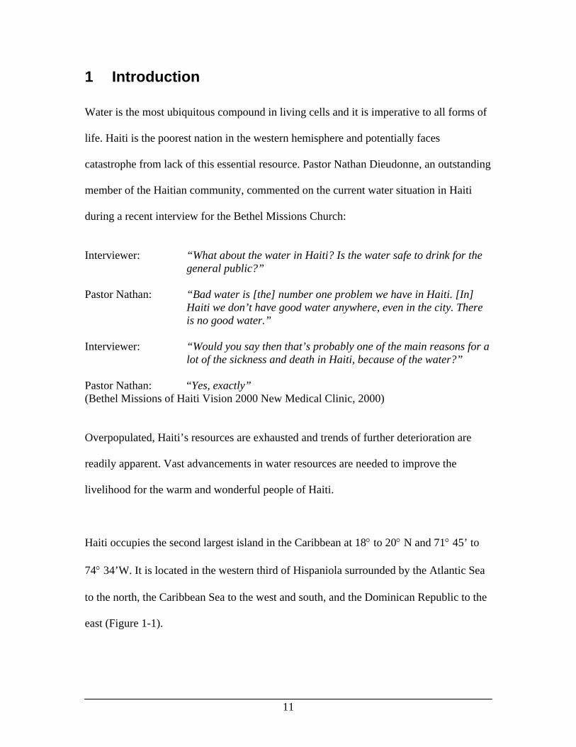
Haiti occupies the second largest island in the Caribbean at 18° to 20° N and 71° 45’ to
74° 34’W. It is located in the western third of Hispaniola surrounded by the Atlantic Sea
to the north, the Caribbean Sea to the west and south, and the Dominican Republic to the
east (Figure 1-1).

12
Figure 1-1. Map of Haiti
Haitians are of approximately 95% African decent and some still practice traditional
voodoo despite the state religion of Catholicism. French is the official language, but 80%
of the population speaks Creole. In 1994, the United States forcibly tried to reinstate
democratically elected president Jean-Bertand Aristide who was removed by the army in
1991. Eventually, the U.S. forces were replaced by a U.N. military mission. The external
fighting and internal struggle for power amongst Aristide’s successors has created chaos.
This has left Haiti without a functioning government since June 1997 and deprived the
country of 150 million dollars in foreign aid (Country Profile: Haiti., 2000). The resulting

13
turmoil has adversely impacted Haiti’s public health, particularly water related issues.
Haitian water is the focus of this study and will now be discussed in more detail.
1.1 Haitian Water Resources
Water in Haiti is generally available from precipitation, rivers and surface water, and
groundwater. All of these resources are intimately related in the hydrologic cycle, which
ultimately provides water for the Haitian community. The amount of water potentially
available from each resource will now be examined followed by the impacts of
deforestation.
1.1.1 Precipitation
Most precipitation is brought by the northeast trade winds with a slight contribution from
easterly winds. Extreme patterns including storms, hurricanes, droughts, and floods are
common. Rainfall can range from less than 30 mm in the northwest to more than 3000
mm in the mountains of the southwest. Orographic factors greatly influence site-specific
rainfall patterns creating the largest precipitation amounts in highly mountainous areas
(USAID, 1985). A rough characterization of rainfall for seven principal areas in Haiti is
(Library of Congress, 1979):
• Northern plain and mountains: More than 1270 mm, with as much as 2540 mm on the higher mountains.
• Northwest: Semi-arid conditions prevail throughout the region, especially around Mole St. Nicolas (508 mm) on the extreme western end of the northern peninsula; Port-de-Paix has about 1524 mm in the mountainous areas.
• Western coast from Mole St. Nicolas to the Cul-de-Sac Plain at Port-au-Prince: Very dry with 500 to 1000 mm of rain; a semi-arid area extending back from the coast over the plain to the mountains covered xerophytic vegetation.
• The island of La Gonave: Similar cover and a rainfall of about 508 to 762 mm.

14
• Artibonite Valley: Lower portion of the valley is a semi-arid region, but rainfall increases rapidly up the valley until it reaches a mean annual level of about 3000 mm; however, about 40 km away in the Cul-de-Sac plain, at about the same altitude, the driest area receives about 500 to 750 mm.
• Eastern part of the mainland between the two peninsulas: The Central Plateau receives about 1016 to 1524 mm of rain.
• Southern Peninsula: Well-watered, with 1524 mm of rain or more in all parts, except the southern slope of the western and a small area near Anse-a-Pitre in the Southeast.
The amount of rainfall that does not infiltrate the ground becomes present in the form of
rivers and surface water.
1.1.2 Rivers and Surface Water
Surface water is used by the majority of Haitians. Most of Haiti’s rivers are short and
swiftly flowing with the exception of the Artibonite River. The broken and steep
landscape gives rise to numerous streams and rivers. However, most of these rivers only
flow during periods of rainfall and few rivers have permanent flow (USAID, 1985). The
principal rivers and corresponding catchment area size are provided by Table 1-1:
Table 1-1. Principal Catchment Areas of Haiti (Library of Congress, 1979)
Main River Average Runoff [m3/s] Length [km] Catchment Area [km2]
Aribonite 34 280 6,862 Riviere de la Grande-Anse 27 90 556 Riviere de l’Estere 19 NA 834 Les Trois Rivieres 12 102 897 Riviere de Cavillon 9 43 380 Grande Riviere du Nord 7 70 312 Riviere du Limbe 6.4 70 312 Riviere Momance 6.4 53 330 Grande Ravine du Sud 3.9 34 330 Grand Riviere du Cul-de-Sac 3.3 NA 290 Riviere l’Acul NA 36 NA

15
Although these flows are presented as averages, they are still highly irregular. The
amount of precipitation that does not contribute to surface water percolates into the soil
and is available as groundwater.
1.1.3 Groundwater
Groundwater is Haiti’s second most important water resource and could become the
primary supply of freshwater in the future. Limestone underlies 80% of the nation
making groundwater readily accessible with well-drilling equipment. Water quality is
high, although hard and slightly saline in some cases. Groundwater is especially abundant
in the coastal plains and these aquifers can yield between 10 to 120 liters a second. Port-
au-Prince and domestic areas such as Cul-de-Sac, Leogane, Carrefour, St-Marc, Cabaret,
Grande-Riviere Du Nord, Limonade, Ouanaminthe, and Aquin widely use groundwater
for domestic purposes (Library of Congress, 1979). Some regions of Haiti contain ample
groundwater but they could be hard to develop as they contain a karstic substratum
(USAID, 1985). HARZA (1979) estimated the potential groundwater resources in 22
select areas summarized by Table 1-2.
Table 1-2. Groundwater Potentials for 22 selected areas (HARZA, 1979)
Region Number of Project Areas
Number of Project Aquifers
No. of Aquifers
Water flow [l/s]
North and North Western 7 13 7 500-685 Artibonite 2 2 - - Southeast Coast 3 5 2 399-1114 South Coast 5 3 2 530+ Central Plains 5 6 1 15-45 Total 22 29 12 1444-1844

16
The onset of any future development of this resource must be carefully evaluated. If
pumping rates exceed groundwater recharge rates, salinization of the freshwater could
occur. Additionally, to obtain optimal benefits from groundwater, as well as surface
water, the effects of deforestation must not only be considered but also remedied.
1.1.4 Impacts of Deforestation
Groundwater and surface water resources depend on the capacity of a watershed to store
water and then gradually release it into rivers and recharge water tables. The ability of a
watershed to retain water depends on its vegetative properties. Surface root structures,
small plants, and dead leaf matter increase overland friction to flow and this allows more
surface water to infiltrate. Deforestation causes a much larger portion of the water to
flow overland, which decreases groundwater base flow. This causes river levels to rise
and fall dramatically as a function of precipitation events. This type of river flow
provides a highly variable and ultimately unreliable source of water. Additionally, loss of
vegetative cover results in significant soil erosion, which degrades both upland and
downstream areas and causing high maintenance costs.
At the beginning of the 16th century, Haiti was covered with lush forests. As of today,
only about 7% of the land is forested. Twelve of the thirty major watersheds were
deforested by 1978. If the rate of deforestation continues, only one pine forest and its
corresponding watershed will remain by the year 2008 (USAID, 1985). The effect of
little vegetative cover on Haiti’s River flows can be seen in Table 1-3.

17
Table 1-3. Deforestation and River Discharges (OAS, 1972; HARZA, 1979; Sheladia Associates, 1983)
River Site of Cleared Land Year [1900]
Mean [m3/s]
Max [m3/s]
Min [m3/s]
Trois Paulin Lacorne 65-67 13.13 527.0 2.65 Pont Gros Morne 23-40; 62-47 6.95 1,500.0 .3 Plaisance 25-40; 62-67 .87 193.0 .01 Limbe Roche a l’Inde 22-40 4.29 458.0 .3 Grande River du Nord Pont Parois 22-40 3.41 9.4 - Massacre Ouanaminthe 22-40 5.34 450.0 .05 Boyaha St. Raphael 22-40 3.41 9.4 - Guayamouc Hinche 26-31 25.52 900.0 .9 Artibonite Mirebalais 22-40 86.9 2,500.0 8.4 Artibonite Pont Sonde 22-40 101.4 850.0 11.1 Estere Pont Estere 65-67 18.76 95.3 1.85 Fer-a-Cheval Pont Petion 23-31 11.85 700.0 .73 Blanche La Gorge 22-40 1.97 200.0 .65 Grise Amt. Bassin Gen. 19-40 3.97 475.0 .31 Pedernales Anse-a-Pitre 29-30 .46 .8 .06 Marigot Peredot 28-30 2.42 79.0 .07 De Jacmel Jacmel 26-31 4.67 800.0 .12 Momance Amont Barrage 20-40 5.88 420.0 .6 Cotes de Fer Cotes de Fer 28-30 .27 7.5.0 0.0 Cavaillon Cavaillon 22-41 9.42 1,035.0 .70 Islet Charpentier 23-31 2.52 500.0 .66 Torbec Torbec 23-31 2.66 188.0 .39 Ravine du Sud Camp Perrin 23-35 4.88 350.0 .28 Grande Anse Passe Ranja 25-31 26.85 60.0 .70 Voldrogue Passe Laraque 28-30 6.07 - .52 Limbe Pont Christophe 22-30 7.1 - .3 Gallois Grison Garde 22-31 .44 - 0.0 Estere Pont Benoit 22-31 3.95 - 0.0 Bois Verrettes 24-31; 33-40 2.58 - .8 La Theme Passe Fine 23-31 4.76 - .64 Montrouis Pont Toussaint 24-30 1.84 - .15 Torcelle Messaye 22-41 1.15 - 0.0 Courjol Bassin Proby 22-39 1.23 - .3 Matheux Arcahaie 22-36 1.50 - .4 Islet Cayes 23-31 2.68 - .64 Acul Carr. Valere 83 3.7 - -

18
There is a 99% average difference between maximum and minimum flow for this data,
which means there are extreme periods of plentiful and deficient water. The goal is to
have a steady source of water available, which may not be possible with the current
amount of deforestation. Significant actions need to be taken to protect and restore the
vegetative cover, and thus the water resources of Haiti’s watersheds. Although Haiti’s
water resources are not known in detail, with the right care, they are believed to be
adequate to meet the needs of the Haitian people. One major task is harnessing these
resources and delivering them to the Haitian people.
1.2 Haitian Water Supply
Two government sections are responsible for managing and developing water resources
in Haiti. The Ministry of Agriculture, through the Services des Ressources en Eau, is in
charge of water resources studies, research, control, and protection. The Ministry of
Public Works provides drinking water through two organizations: Centrale Autonome
Metropolitaine d’Eau Potable (CAMEP) for the metropolitan area, and Service Nationale
d’Eau Potable (SNEP) for the remainder of the country. In reality, there is little control
over the use of water resources and several other government and non-government
organizations administer water supply programs (USAID, 1985).
In 1978, there were 40 domestic water supply systems in the country serving 700,000
people, or roughly 15 percent of the population (HARZA, 1979). The existing water
supply programs are the result of investments by government agencies, and bilateral and
multilateral cooperation organizations. In 1984, the government devoted 4 percent of the

19
budget to potable water projects and this contribution was financed at 84 percent by
external assistance (USAID, 1984).
CAMEP serves Port-au-Prince, Petionville, Carrefour, and Delmas. CAMEP supplies its
customers from 17 springs and 3 wells from the Cul-de-Sac (USAID, 1985). The upkeep
of these structures and associated distribution pipes leave much to be desired. Water loss
from the pipes is estimated from between 50 and 70 percent (DATPE, 1984; Fass, 1982).
All of these sources, with the exception of Doco Spring, have disinfection units but they
are usually not operational. CAMEP nominally serves about 500,000 people through
40,000 connections and 80 functioning standpipes. In actuality, only about 80,000 people
utilize CAMEP as their legal source of water. Approximately 300,000 people obtain
water from private vendors, 100,000 share a connection with a subscriber, and about
40,000 illegally tap into CAMEP’s pipes (USAID, 1985).
SNEP is responsible for the construction, operation, and maintenance of all water supply
systems outside the metropolitan area. SNEP’s finances are severely limited it but has
received assistance from UNICEF, WHO, The World Bank, Inter American
Development Bank, German Foundation for Technical Assistance, and USAID (USAID,
1985). SNEP has 185 water supply systems in operation, serving a total population of
700,000. Most of these systems are capped springs. Community systems range from a
dug or bored well with a hand pump serving about 200 people, to house connections and
public fountains that serve about 60,000 (USAID, 1985). Several organizations helped
finance or physically participated in the construction of these systems: IDB, Organization

20
pour le Development du Nord, and Department de la Sante Publique et de la Population
at the Ministry of Health. In addition, several non-governmental organizations made vital
contributions: CARE, World Church Service, Missionary Church Association, German
Foundation for Technical Assistance, and Canadian Agency for International
Development. A summary of water supply systems is given by Table 1-4.
Table 1-4. Water Supply Systems (HARZA, 1979; USAID, 1985)
Service Area 1978 1985 1991 Metropolitan Area 460,000 500,000 600,000 Balance of West Department 60,000 150,000 290,000 Southeast Department 14,600 30,000 80,000 North Department 30,900 150,000 290,000 Northeast Department 5,400 15,000 90,000 Artibonite Department 51,000 160,000 360,000 Center Department 17,500 30,000 80,000 Northwest Department 36,300 40,000 130,000 South Department 24,000 75,000 230,000 Grand’ Anse Department 14,900 50,000 150,000
Total Served 715,000 1,200,00 2,300,000 Total Population 4,750,000 5,200,000 5,600,000 Percent Served 15% 23% 41%
1985 Systems under POCHEP and UNICEF
Service Area Population Served Service Area Population Served North (18) 15,200 West (50) 27,400 Northeast (0) 0 Southwest (3) 4,900 Artibonite (38) 34,100 South (18) 23,100 Center (4) 6,500 Grande Anse (8) 9,500 Northwest (0) 0 Subtotal (139) 120,700
A major problem with these water supply systems is there is no presence of national
drinking water supply standards. The managers of CAMEP, SNEP, Public Hygiene
Division, and Sanitation Office indicate the main concern is bacteriological

21
contamination. It is generally agreed that there is enough water for drinking purposes and
the real issue is to develop the quality of the resource (DATPE, 1984).
1.3 Haitian Water Quality
Water-related diseases run rampant in Haiti. CAMEP and SNEP water is theoretically
disinfected before distribution. However, treatment is very erratic due to breakdowns and
lack of backup supplies. Surface water and groundwater from uncapped springs is
considered unsafe due to the high risk of contamination. Water from private vendors can
pose a risk of disease because it is not disinfected and the sources are unprotected. Even
bottled water cannot be guaranteed, as there is potential contamination during the
shipping process. Essentially, there is no controlled potable water in Haiti and every
source could contain pathogens (DATPE, 1984).
Waterborne pathogens are capable of causing illness depending on the dose and physical
condition of the exposed individual. Infectious organisms found in water may be
discharged by human beings who are carriers of a disease. Pathogenic organisms include
bacteria, viruses, protozoa, and helminthes, which can all cause a wide array of diseases.
Table 1-5 depicts common perilous organisms found in water and their corresponding
disease.

22
Table 1-5. Infectious Agents Present in Raw Domestic Wastewater (Metcalf & Eddy, 1991)
Organism Disease Remarks Bacteria Escherichia coli Gastroenteritis Diarrhea Legionella pneumophila Legionellosis Acute respiratory illness Leptospira Leptospirosis Jaundice, fever (Weil's disease) Salmonella typhi Typhoid fever High fever, diarrhea, ulceration Salmonella Salmonellosis Food poisoning Shigella Shigellosis Bacillary Dysentery Vibrio cholerae Cholera Extremely heavy diarrhea, dehydration Yersinia enterolitica Yersinosis Diarrhea Viruses Adenovirus (31 types) Respiratory disease Enteroviruses (67 types)
Gastroenteritis, heart anomalies, meningitis
Hepatitis A Infectious hepatitis Jaundice, fever Norwalk agent Gastroenteritis Vomiting Reovirus Gastroenteritis Rotavirus Gastroenteritis Protozoa Balantidium coli Balanticliasis Diarrhea, dysentery Cryptosporidium Cryptosporidiosis Diarrhea Entamoeba histolytica Amebiasis (amoebic dysentery) Prolonged diarrhea with bleeding, abscesses
of the liver and small intestine Giardia lamblia Giardiasis Mild to severe diarrhea, nausea, indigestion Helminths Ascaris lumbricoides Ascariasis Roundworm infestation Enterobius vericularis Enterobiasis Pinworm Fasciola hepatica Fascioliasis Sheep liver fluke Hymenolepis nana Hymenolepiasis Dwarf tapeworm Taenia saginata Taeniasis Beef tapeworm Taenia solium Taeniasis Pork tapeworm Trichuris trichiura Trichuriasis Whipworm

23
These infectious organisms can have highly deleterious impacts on community members.
Table 1-6 shows there were several thousand cases of water related diseases reported in
1980 (CONADEPA, 1984).
Table 1-6. Some Reported Cases of Water Related Diseases in 1980 (CONADEPA, 1984)
Area Population Diarrhea Intestinal Infections Typhoid Cases /1000 Cases /1000 Cases /1000
Port-au-Prince 650,000 6608 10.2 4694 7.2 460 .7 Gonaives 33,000 225 7.7 167 5.1 11 .3 Port-de-Paix 15,000 455 30.3 2171 145 114 7.6 Hinche 10,000 694 69.4 738 74 100 10.0 St. Marc 23,000 851 37.0 314 13.7 266 11.6 Petit Goave 7,000 294 42.0 1357 194 2 .3 Belladere 2,500 875 350.0 272 109 68 27.2 Jacmel 13,000 320 24.6 152 11.7 87 6.7 North Dept. 560,000 3145 5.6 6819 12.2 141 .3 South Dept. 500,000 1909 3.8 2380 4.8 462 .9
The actual numbers of diarrhea and intestinal infections are much higher as many
occurrences are never reported. In 1979, diarrhea alone caused the death of 9% of the
babies less than one year of age (USAID, 1984). A study from 1994 to 1995 found nearly
one-half of all deaths occurred within the first five years of life. Additional statistics
indicate, approximately 74 out of 1,000 births die before one year of age and 131 never
reach five years of age (PAHO, 1999). The National Health Survey conducted a survey
from 1987-1994 and found that the incidence of diarrhea was about 47.7% in
6-to-11-month-old infants. Diarrheal diseases are the leading cause of illness and death in
children under five years of age, and are often associated with malnutrition and acute
respiratory infections (PAHO, 1999). These daunting statistics make water quality the
biggest water resource issue in Haiti. If correctly managed, there is an ample amount of

24
water to meet the needs of the Haitians but they need an easy and economical way to
destroy waterborne pathogens.
1.4 Point-of-Use Water Treatment
In developed countries, pathogens are typically destroyed by elaborate centralized water
treatment plants. Unfortunately, it is not financially possible to upgrade to conventional
water treatment technologies in Haiti. As a more plausible alternative, low-cost
point-of-use disinfection technologies can treat water and are more economically
realistic. The choice of a point-of-use water technique should fulfill the following criteria
(Lehr et al., 1980; Shultz et al., 1984):
1. Effective on many types and large numbers of pathogens 2. Should perform regardless of water fluctuations 3. Must operate in appropriate pH and temperature range 4. Should not make the water toxic or unpalatable 5. Should be safe and easy to handle 6. Any chemical concentrations should be minor 7. Must provide residual protection against possible recontamination 8. Units must be affordable to all 9. Should be adaptable to local conditions and variations 10. Specialized equipment should be produced locally 11. Must be accepted by local traditions, customs, and cultural standards 12. Must comply with national sanitation and pollution policies
Common point-of-use disinfection techniques such as chlorination, boiling, and filtration
can be successful but have associated problems. Chlorine is the most widespread
disinfection method and will be discussed in the most detail.
Chlorine’s most important attributes are its germicidal potency and persistence in water
distribution systems. Chlorination uses chlorine gas, Cl2; sodium hypochlorite, NaOCl; or

25
calcium hypochlorite, Ca(OCl)2. These forms of chlorine act as powerful oxidizing
agents that damage vital cell structures. The key reaction of the dissolution of chlorine
gas in water is as follows:
2 2Cl H O HOCl H Cl+ −+ + +! !!! !!
HOCl H OCl+ −+! !!! !!
The hypochlorous acid formed, HOCl, is the prime disinfection agent. The protonation of
hypochlorous acid depends on pH and yields the less effective hypochlorite, OCl−
.
Together the HOCl and OCl − make up the free available chlorine, which is most useful
for disinfection. In addition, chlorine based compounds can form long lasting residual
compounds to provide continual disinfection (Metcalf and Eddy, 1991).
Chlorination has been controversial for decades, as consumers do not like the associated
odor and taste. Chlorine also reacts with natural aquatic substances to produce
disinfection byproducts such as trihalomethanes (Gibbons and Laha, 1999). Animal and
epidemiological studies suggest these byproducts can cause adverse health affects, are
possibly carcinogenic, and are linked to an increased risk of birth defects (Trussell 1999;
Per Magnus et al., 1999). Furthermore, chlorine poses additional problems such as
reliable supply, timely distribution, and correct dosage (Wegelin et al., 1994).
Other household disinfection mechanisms include boiling the water and filtering. In
Haiti, boiling water uses energy in the form of firewood, which is no longer possible due
to extensive deforestation. Filtration is often unaffordable and is subject to frequent

26
clogging and leaking. In addition, filtering typically requires additional disinfection steps.
These problems call for the development of an alternative disinfection technology that is
effective, practical, and simple enough to be applied by individuals at the household
level. Under the right conditions, solar water disinfection, or SODIS, may be that
alternative.

27
Section II: SODIS for Point of Use Water Treatment

28
2 SODIS: Solar Water Disinfection
2.1 SODIS Introduction and Development
SODIS uses the sun’s energy to provide an economically feasible means of providing
safe drinking water. This treatment process produces disease-free water by filling
transparent containers and exposing them to sunlight:
Figure 2-1. SODIS Overview
The science behind SODIS will be discussed after a little background. This technology
was pioneered in the late 1970s by Acra et al. at the American University of Beirut,
Lebanon, to find an inexpensive disinfection method for oral rehydration solutions (Acra
et al., 1984). Their exciting results gave birth to a new disinfection technique.

29
Consequently, a workshop on SODIS was held in Montreal in 1988 (Lawand et al.,
1988), and SANDEC/EAWAG (Swiss Federal Institute for Environmental Science and
Technology) started to investigate the SODIS process in 1991. Their findings were
encouraging and field-tests where launched to include several countries: Columbia,
Bolivia, Burkina Faso, Togo, Indonesia, Thailand, and China (EAWAG/SANDEC,
1998). The most alluring aspect of this technology is the low investment costs of plastic
bottles and the disinfection energy that is provided free of charge by the sun.
2.2 Solar Radiation and Disinfection
SODIS uses the destructive power of different bands of the electromagnetic spectrum to
destroy pathogens. Photodynamic inactivation of microorganisms was first demonstrated
by Raab in 1900. The sun emits energy in the form of electromagnetic radiation that
covers the ultraviolet, visible, and infrared range. The most important bandwidths for
SODIS are the UV-A, red, and infrared, which are shown in relation to the electromagnet
spectrum by Figure 2-2.
Figure 2-2. Important Components of the Electromagnetic Spectrum (Solomon, 1996)

30
Recent studies have shown that UV-A light is the main bandwidth involved in the
eradication of microorganisms (Acra et al, 1984; Acra et al., 1990; Reed et al., 1997;
McGuigan et al., 1998). UV-A has direct effects on DNA and forms highly destructive
oxygen species as a secondary product. In addition, water strongly absorbs red and
infrared light creating heat, which results in pasteurization. Figure 2-3 shows the
combined effects of UV-A and water temperature on coliform bacteria.
Figure 2-3. UV-A and Temperature Effect on Fecal Coliform (EAWAG/SANDEC, Technical Notes).
Microbial inactivation is contingent on the disinfection mechanisms of DNA alteration,
photo-oxidative destruction, and thermal pasteurization damaging cellular defenses. This
concept for each process will now be discussed further.
2.3 DNA Alteration by UV
To assure pathogenic organisms are eradicated, DNA must be damaged faster than
microbes can repair it. DNA has a maximum UV absorbance at around 260 nm that
causes mutagenesis and results in cellular death (Raven and Johnson, 1996). Absorbed
UV light causes adjacent thymine bases to covalently bond together, forming thymine
dimers:

31
Figure 2-4. Formation of Thymine Dimers (Raven and Johnson, 1996; Mathews and Van Holde, 1996)
When this damaged DNA replicates, nucleotides do not complementary base pair with
the thymine dimers and this terminates replication. Organisms may also replace thymine
dimers with faulty base pairs, which causes mutations, leads to faulty protein synthesis,
and may result in death.
The effect of thymine dimer formation may be reversed to some extent by exposure to
visible light in a process called photoreactivation. Visible light can activate the enzyme
DNA photolyase that breaks the bond joining the thymine bases. DNA can also be
repaired by excision, where DNA polymerase and DNA ligase cut out damaged DNA and
replace it with a stretch of error-free DNA (Mathews and Van Holde, 1996).
When DNA damage is too extensive for photoreactivation and excision mechanisms, the
cell coordinates the expression of a large number of unlinked genes, which enhance
capacity for DNA repair and inhibit cell division. This orchestrated activation of diverse

32
metabolic functions to repair damaged DNA damage has been called the SOS response
(Mathews and Van Holde, 1996). The manifestation of the SOS response eventually leads
to DNA repair and returns the cell to its normal growth cycle.
Extreme UV-resistance of some bacteria is a result of efficient DNA repair machinery
along with powerful scavenging activity of cells toward various reactive oxygen species
generated by UV irradiation (reactive oxygen species are discussed in the next section).
To ensure UV-A radiation overpowers pathogenic cellular defense mechanisms, a
sunlight intensity of 500 W/m2 should be applied for 3 to 5 hours to induce lethal effects
(SODIS News No. 1, 1998). UV-A also creates highly reactive oxygen species as a
secondary disinfection product in a process called photo-oxidative disinfection.
2.4 Photo-Oxidative Disinfection
UV-induced reactive oxygen species can be lethal if they are present in numbers higher
than the organism is capable of attenuating. Natural dissolved organic matter can absorb
ultraviolet radiation to induce photochemical reactions (Miller, 1998). The energy
transfer of a high-energy photon to absorbing molecule produces highly reactive species
such as superoxides (O2-), hydrogen peroxides (H2O2), and hydroxyl radicals (OH•)
(Stumm and Morgan, 1995; Miller 1998). These highly reactive species in turn oxidize
microbial cellular components such as nucleic acids, enzymes, and membrane lipids,
which kill the microorganisms (McGuigan et al., 1999; Reed 1996; Reed 1997).

33
In their defense, microorganisms have evolved powerful scavenging activity toward
various reactive oxygen species. (Yun et al., 2000; Fridovich, 1988; Halliwell, and
Gutteridge, 1999). A common defense against superoxide is carried out by a group of
enzymes called superoxide dismutase. Superoxide dismutase catalyzes the following
reaction, which decreases the lifetime of superoxide by a factor of 109 (Fridovich, 1998):
2 2 2 2 22O O H H O O− − ++ + +! !!! !!
Microbes cope with hydrogen peroxides using two groups of enzymes called catalases
and peroxidases. Catalases eliminate hydrogen peroxide by:
2 2 2 22 2H O O H O+! !!! !!
while peroxidases uses the reducing power of NADH:
2 2 22 2 2H O NADH NAD H O++ +! !!! !!
In addition to superoxide dismutases, catalases, and peroxidase, there is an additional
orchestrated defense observed in E. coli involving the SoxRS and OxyR regulons. When
activated, these regulons express several genes to provide additional defense (Fridovich,
1998).
Superoxide and hydrogen peroxide are not themselves dramatically devastating, but they
can produce hydroxyl radicals, which form a juggernaut of oxidative power, in two ways:
2 2 2
3 22 2
2 32 2
1.
2 .
2 .
H O e H H O OH
a M O M O
b M H O OH M OH
where M is a metal
− +
−+ +
+ − +
+ + +
+ +
+ + +
! !! !! !!
! !!! !!
! !! !! !!

34
After the hydroxyl radical if formed, it reacts extremely fast with almost every type of
molecule found in living cells causing tremendous damage.
For photo-oxidative disinfection to occur, sufficient levels of oxygen need to be initially
present. This was demonstrated by Reed in 1997 by comparing aerobic and anaerobic
inactivation rates E. coli and Ent. faecalis using solar disinfection.
Figure 2-5. Aerobic vs. Anaerobic Microbial Inactivation (Reed, 1997).
The aerobic rates of disinfection (circles) are much faster than the anaerobic rates
(squares), indicating that the presence of oxygen is essential for the rapid solar
destruction of E. coli and Ent. faecalis.

35
Reed’s experiments demonstrated the importance of oxygen to SODIS. This desired
aeration can be achieved on a practical level by vigorously shaking the SODIS containers
before sunlight exposure. This is especially important for stagnant water sources where
the levels of dissolved oxygen are questionable (EAWAG/SANDEC, Technical Notes).
2.5 Thermal Inactivation
Thermal effects can act synergistically in the disinfection process if they can overcome
microbial heat resistance. As temperatures rise past the maximum growth value, it
becomes difficult for proteins to form their proper structures and it causes already formed
proteins to unfold. Denatured proteins do not function properly and may eventually kill
the organism (Brock, 2000).
Microorganisms have special chaperone proteins that are especially suited for elevated
temperatures due to better hydrogen bonding, superior hydrophobic packing, and
enhanced secondary structure. These heat shock proteins are present in low
concentrations under normal conditions, but are expressed at high levels when exposed to
a sudden increase in temperature. These proteins help keep other proteins functional and
can cause heat resistance (Brock, 2000). The efficacy of these heat-shock proteins
determines how much temperature an organism can withstand before heat inactivation.
It has been observed that water temperatures between 20 and 40 ° C do not affect the
inactivation of E.coli by sunlight (Wegelin et al., 1994). However, synergistic effects are
observed at a water temperature of 45 ° C (McGuigan et al., 1998). Compared to lower
36
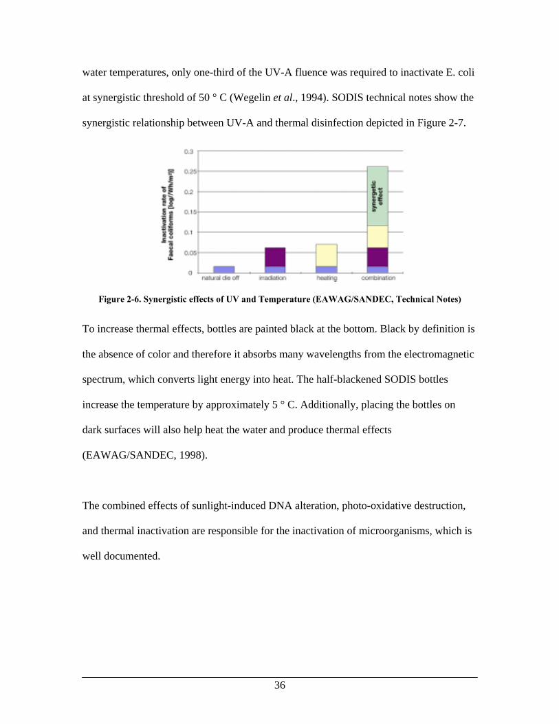
water temperatures, only one-third of the UV-A fluence was required to inactivate E. coli
at synergistic threshold of 50 ° C (Wegelin et al., 1994). SODIS technical notes show the
synergistic relationship between UV-A and thermal disinfection depicted in Figure 2-7.
Figure 2-6. Synergistic effects of UV and Temperature (EAWAG/SANDEC, Technical Notes)
To increase thermal effects, bottles are painted black at the bottom. Black by definition is
the absence of color and therefore it absorbs many wavelengths from the electromagnetic
spectrum, which converts light energy into heat. The half-blackened SODIS bottles
increase the temperature by approximately 5 ° C. Additionally, placing the bottles on
dark surfaces will also help heat the water and produce thermal effects
(EAWAG/SANDEC, 1998).
The combined effects of sunlight-induced DNA alteration, photo-oxidative destruction,
and thermal inactivation are responsible for the inactivation of microorganisms, which is
well documented.

37
2.6 Inactivation of Indicator Organisms and Pathogens
SODIS efficacy is usually established through the inactivation of indicator organisms, but
effects on actual pathogens have also been investigated. A brief overview of indicator
organisms will be given, as they are the most commonly used gauges of SODIS success.
This will be followed by a tabulation of microorganisms that are inactivated by SODIS
and a table of the heat sensitivities of some pathogens will also be provided, as thermal
effects are an important aspect of the SODIS process.
2.6.1 Indicator Organisms
A person discharges billions of organisms per day and most of the pathogenic fraction of
these organisms is difficult to isolate and identify. Consequently, the presence of easily
identifiable organisms is used to suggest the existence of pathogenic ones. The
characteristics of an ideal indicator organism are shown in Table 2-1.
Table 2-1. Criteria for an Ideal Indicator Organism (Maier et al., 2000)
Used for all types of water Present whenever enteric pathogens are present Should have a reasonably longer survival rate than pathogens Should not grow in water Testing method should be easy to perform Density should allude to extent of fecal pollution Should be a member of the microflora of warm-blooded animals
Unfortunately, no single group of organism meets all of the above criteria. Consequently,
multiple indicator organism groups are often used. The two most common ones are total
and fecal coliform.

38
2.6.1.1 Total Coliform
Coliform bacteria include the genera Escherichia, Enterobactor, and Klebsiella and are
characteristically facultatively anaerobic, gram-negative, non-spore-forming, rod-shaped
bacteria that can ferment lactose to produces gas (Maier et al., 2000). Traditionally,
coliform quantity has served as the standard to gauge water quality with respect to
pathogens.
Experience has shown that the absence of coliform bacteria in 100 ml of drinking water
will prevent enteric diseases. Two realizations have been made to support this
observation. First, relatively few individuals excrete pathogens while the entire
population contributes coliform to the waste stream. Therefore, the number of coliform
should far exceed the number of pathogens as shown for infectious viruses by Table 2-2.
Table 2-2.Virus-Coliform Ratios for Sewage and Polluted Surface Waters (Masters, 1997)
Virus Coliform Virus/Coliform Ratio Sewage 500/100 ml 46*106/100 ml 1:92,000
Polluted Surface Water 1/500 ml 5*104/100 ml 1:50,000
Second, the survival rate of pathogens outside of the host is much lower than the survival
rate of coliform bacteria. The combination of these two factors statistically suggests that
it is extremely unlikely to have water containing pathogens without numerous coliform.
However, coliform bacteria have characteristics that make them less than an ideal
indicator organism: regrowth in tropical waters, suppression of numbers by background

39
bacterial growth, some eukaryotic organisms like Giardia can survive considerably
longer outside their host, and not all coliform are of fecal origin.
2.6.1.2 Fecal Coliform and E. coli
To help eliminate possible false positives, coliform of only fecal origin can be used.
These organisms consist of the Escherichi and Klebsiella genera. These coliforms can
ferment lactose to produce both acid and gas at 44.5 ° C within 24 hours (Maier et al.,
2000). It has been suggested that E. coli be used as an indicator organism as it can readily
be distinguished from other members of the coliform group. However, E. coli cannot be
differentiated between human and animal origin. Despite these limitations, fecal coliform
bacteria have proven invaluable in assessing drinking water quality as shown by Table
2-3:
Table 2-3. Indicator Organisms Used in Establishing Performance Criteria for Various Water Use (Metcalf and Eddy, 1991)
Water Use Indicator Organisms Drinking Water Total coliform Freshwater Recreation Fecal coliform, E. coli, Enterococci Saltwater Recreation Fecal coliform, total coliform, Enterococci Shellfish Growing Areas Total coliform, fecal coliform Agricultural irrigation Total coliform (for reclaimed water) Wastewater effluent disinfection Total coliform, fecal coliform
In 1984, Acra demonstrated that E. coli serves as good indicator organism for SODIS as
it is more resistant to the lethal effects of sunlight than other bacteria. Coliform bacteria
have become the general standard in assessing microbial water quality but many other
organisms have been put to the SODIS test.

40
2.6.2 Inactivation of Specific Microorganisms and Heat Sensitivity
Table 2-4 is a list of microorganisms that have been inactivated by the SODIS process. It
is not comprehensive and the references for coliform bacteria are far more extensive.
However, it demonstrates that many different microorganisms are sensitive to the SODIS
method.
Table 2-4. SODIS Inactivation of Microorganisms
Microorganism Reference: E. coli Wegelin et al., 1994 Fecal Coliform Sommer, 1997 Vibrio Cholera Sommer, 1997 Vibrio Cholera New Scientist Magazine, 2000 P. aerugenosa Acra et al., 1984 S. flexneri Acra et al., 1984 S. typhi Acra et al., 1984 S. enteritidis Acra et al., 1984 S. paratyphi Acra et al., 1984 Aspergillus niger Acra et al., 1984 Aspergillus flavus Acra et al., 1984 Candida Acra et al., 1984 Str. Faecalis Wegelin et al., 1994 Penicillium Acra et al., 1984 Polio Virus Cubbage et al.,1979 Bacteriophage MS2 Kapuscinski and Mitchell, 1982 Enterocci Wegelin et al., 1994 Bacteriophage f2 Wegelin et al., 1994 Encephalomyocarditis virus Wegelin et al., 1994 Rotavirus Wegelin et al., 1994 Cryptosporidium∗ Bukhari et al., 1999; Clancy et al., 1998 Cryptosporidium New Scientist Magazine, 2000 Giardia Muris∗ Craik et al., 2000
∗Found under a UV lamp measured in the UV-C range. Although UV-C is not found in sunlight, it suggests these organisms would be sensitive to the UV-A portion of sunlight.

41
While this list does not address all of the important pathogens, there is active research to
investigate important pathogens such as Giardia (SODIS Conference Synthesis, 1999).
Some additional insight to other microorganisms could be gained by examining their
thermal sensitivities, as thermal inactivation of microorganisms is a very important
process in SODIS. Table 2-5 shows the heat sensitivities of several infectious organisms.
Table 2-5. Thermal Destruction of Microorganisms (Feachem et al., 1983)
Time and Temperature for 100% destruction Microorganism 1 min 6 min 60 min Enteroviruses 62 °C Rotaviruses 63 °C for 30 min Salmonellae 62 °C 58 °C Shigella 61 °C 54 °C Vibrio Cholera 45 °C Entamoeba Histolytica cysts 57 °C 54 °C 50 °C Giardia Cysts 57 °C 54 °C 50 °C Hookworm eggs and larvae 62 °C 51 °C Ascaris eggs 68 °C 62 °C 57 °C Schistosomas eggs 60 °C 55 °C 50 °C Taenia eggs 65 °C 57 °C 51 °C
The inactivation of microorganisms by the SODIS process is fairly well established.
However, there has been some concern of secondary UV effects enhancing bacterial
growth and the possible regrowth of enteric pathogens. These issues will now be
examined.

42
2.7 UV-Enhanced Bacterial Growth and Bacterial Regrowth
Studies have shown that exposures of UV radiation can actually increase indigenous
concentrations of bacteria (Moran and Zepp, 1997; Bertilsson et al., 1999; Lindell et al.,
1995). Solar UV radiation may alter the chemistry of dissolved humic substances in water
to produce lower molecular weight organic compounds, which serve as substrate for
microorganisms (Mopper and Stahovec, 1986; Kieber et al., 1989). Additionally,
photochemical reactions can generate free ammonium in humic and natural waters
(Bushaw et al., 1996; Gao and Zepp, 1998). These effects of liberated food and nutrients
can enhance bacterial growth. Furthermore, studies have shown that E. coli can regrow
after UV-C inactivation (Mechsner and Fleischmann, 1990; Mechsner et al., 1991;
Mechsner and Fleischmann, 1992). These various factors suggest that it may be possible
for pathogens to be present after short-term storage if given enough time to regenerate.
Wegelin et al. (1994) examined various aspects of microbial regrowth to show that
sunlight and UV-C do not fully kill bacteria mixtures beyond regrowth, and E. coli could
regenerate from UV-C radiation. However, there was no revival observed for E. coli
inactivated by the SODIS process (Figure 2-7).

43
Figure 2-7. Bacterial Regrowth (Wegelin et al., 1994)
Wegelin et al. state that the difference in E. coli regrowth can be attributed to the
relatively longer exposure time required to inactivate the cells with solar radiation when
compared to the UV-C fluence. For the study conducted by Wegelin et al. (1994), the
regrowth of natural bacteria from sunlight was attributed to the resistant saprophytic
bacteria and their spores.
An interesting question for further research is, in general, why can indigenous microbial
populations regenerate from the SODIS process while enteric pathogens are permanently
inactivated? One can speculate that the indigenous aquatic microorganisms have much
more developed DNA repair and reactive oxygen species defense mechanisms (as
previously described). Evolution in an environment that has frequent exposure to UV and
reactive oxygen species would cause the microorganisms that are most resistant to these

44
adverse effects to be most successful. This would cause microbial populations indigenous
to aquatic systems to have greater UV and reactive oxygen species resistance. However,
enteric pathogens have evolved in the dark anaerobic human gut and, consequently, there
would be no selective pressure to produce such developed repair mechanisms against UV
and reactive oxygen species. Consequently, when enteric pathogens are exposed to the
SODIS process, they are inactivated while the indigenous populations can revive. Despite
any bacterial revival, the aim of SODIS is to produce a pathogen-free source of water and
not a sterile solution, which the study conducted by Wegelin et al. (1994) demonstrated.
The science behind SODIS has been discussed. However, SODIS efficacy is highly
dependent on site-specific conditions. These conditions along with some practical aspects
must be considered before applying SODIS.

45
3 Important SODIS Variables
SODIS operates on the principle that sunlight-induced DNA alteration, photo-oxidative
destruction, and thermal effects will inactivate microorganisms. For these parameters to
be effective, the environment must be sunny and hot enough, the water must be clear
enough to allow the light to penetrate, and the type of bottle being used must not
substantially hinder these processes. In addition, for this technology to become a reality,
people must be able to afford it, and they must believe in it, or it would never be applied.
Haiti’s climate as it relates to SODIS will be discussed, including an approach to simulate
sunshine intensities. This will be followed by a discussion of the social acceptance
observed in different parts of the world along with economic considerations.
3.1 Haitian Climate
Assuming there is adequate oxygen to mix into the water, the two most influential
variables affecting SODIS efficacy are sunshine and temperature. These two parameters
are a function of seasonal and geographical climate variation. To assess these factors,
Haiti is discretized into seven sections that correspond to the degree latitude and
longitude data obtained from NASA Langley Atmospheric Sciences Data Center (Figure
3-1).

46
Figure 3-1. Discretization of Haiti (NASA Langley Research Center Atmospheric Sciences Data
Center, 2001)
Based on this discretization, seasonal Haitian sunshine and temperature will be examined
followed by influences of topography.
3.1.1 Haitian Sunshine
The sun is a giant fusion reactor that destroys matter to yield energy in the form of
electromagnetic radiation. The earth is partially shielded from solar radiation by
absorption, scattering, and reflection in the stratosphere and troposphere (Brooks and
Miller, 1963; McVeigh, 1977; Sabins, 1978; Michaels, 1979; WHO, 1979).
Stratospheric ozone strongly absorbs shorter wavelength radiation while its affinity
decreases rapidly with higher wavelengths. This high-energy absorption blocks the earth
4 5 6 7321

47
from UV-C and only allows a fraction of UV-B and UV-A to reach ground level (Acra,
1990). Solar attenuation in the troposphere is primarily caused by clouds, dust, smoke,
haze, smog, and various gases. Tropospheric scattering highly depends on particle size
and produces both selective and nonselective scattering. Selective scattering is caused by
smoke, fumes, haze, and gas molecules that are smaller than or equal to the incident
radiation wavelength. This type of scattering affects shorter wavelengths and is more
severe for polluted atmospheres. Nonselective scattering is caused by dust, fog, and cloud
particles with sizes more than 10 times the wavelength of the incident radiation. In
addition, thin clouds may reflect less than 20% of the incident solar radiation, while thick
clouds may reflect over 80% of all radiation (Acra, 1990).
Atmospheric attenuation causes the amount of solar radiation that reaches the earth’s
surface to be highly dependent on the path length through the atmosphere. This path
length is a function of the earth’s tilt, rotation, and slightly elliptical orbit. As the earth
rotates around the sun, its axis is tilted constantly at 23.47°. During summer, the
hemisphere tilts towards the sun, which causes the radiation to be more perpendicular and
of greater duration. In winter, the hemisphere tilts away from the sun creating a longer
atmospheric path and shorter days. A gradual transition occurs between these two
extremes, giving seasonal changes. NASA Langley Atmospheric Sciences Data Center
provides visualization for Haiti of a 10-year average monthly value of total daily
radiation (Figure 3-2).

48
Figure 3-2. Average Monthly Value of Total Daily Radiation (NASA Langley Research Center Atmospheric Sciences Data Center, 2001)
The monthly amount of total surface radiation provides important information for
assessing SODIS. However, recommendations for SODIS are based on a threshold of

49
sunlight intensities rather than the total amount of energy received. Fortunately, these two
entities are intimately related and can be sufficiently described by mathematical models.
3.1.2 Mathematical Development of Sunshine Simulation
SODIS efficacy depends on an adequate duration of sunshine radiation. It has been
deduced that an intensity of 500 W/m2 should be available for 3 to 5 hours for effective
disinfection (SODIS News No. 1, 1998). A value of at least 5 hours of sunshine above
500 W/m2 will be used as a conservative threshold. Many areas of the world in need of
SODIS are developing countries, and consequently, do not have meteorological data on
sunshine intensity profiles. However, NASA Langley Atmospheric Sciences Data Center
provides web accessible data on the 10-year average, minimum, and maximum amount of
total energy received for a representative day of each month. This data has a spatial
resolution of one-degree latitude and longitude for the entire world. Quantitative
knowledge of the total amount of daily energy received, allows for the simulation of daily
sunshine intensity profile. This information can then be used to calculate the average,
minimum, and maximum intensity for the peak five hours of sunshine to get a first
approximation of whether SODIS would be applicable for any given month. This
technique will be applied to simulate Haitian sunshine but could be easily extended to
simulate monthly sunshine values for anywhere in the world.
The general approach is to calculate the day length based on location and time of the
year, which involves the earth’s declination angle and sunrise angle. Next, the sun’s hour
angle relative to the location is obtained. This combined information is then used to
determine what fraction of the total radiation is received at a given hour, ultimately

50
generating daily sunshine profile. The meanings and calculations for each necessary
parameter will now be discussed.
The declination, dω , is the angular distance at solar noon between the sun and the
equator, referenced as north positive. Declination changes with date and is independent of
location. It has maximum absolute value of 23.45 degrees during the summer and winter
solstice and 0 degrees on the equinoxes. It can be approximated for a specific Julian day
from the equation given by Cooper (1969).
( )360 28423.45sin
365
:[ ]
( 1)
Jdayd
d
Jday
n
wheredeclination angle
n julian day number of days after January
ω
ω
+=
= °=
(1.1)
For practical purposes, Duffie and Beckman (1980) provide a table with declination
angles that are representative of each month:
Table 3-1. Recommended average day for each month (Duffie and Beckman, 1980)
Month Date Julian Day Declination, [ ],dω °
January 17 17 -20.9 February 16 47 -13.0 March 16 75 -2.4 April 15 105 9.4 May 15 135 18.8 June 11 162 23.1 July 17 198 21.2 August 16 228 13.5 September 15 258 2.2 October 15 288 -9.6 November 14 318 -18.9 December 10 334 -23.0
*Values do not account for leap year; correct by adding 1 to months from March onward. Declination will also change slightly

51
The hour-angle, tω , is the angular displacement of the sun east or west of the local
meridian due to rotation of the earth at 15° per hour. The hour-angle can be calculated
from the following equation (Brock, 1980).
( 12)15
:- [ ]
[ ]
t
t
t
wherehour angle
t time from midnight hr
ω
ω
= −
= °=
(1.2)
The sunset or sunrise hour-angle, sω , is the hour-angle when the sun’s center reaches the
horizon and can be computed if the location’s latitude, L, and current declination, dω , are
known (Milankovitch, 1930).
( ) ( )( )1cos tan tan
:[ ]
[ ]
s d
s
L
wheresunrise or sunset angle
L latitude
ω ω
ω
−= −
= °= °
(1.3)
From the sunset angle, the day length, Dl , can be calculated:
2
15
:[ ]
sDl
whereDl day length hr
ω =
=
(1.4)
The total daily average solar radiation, daI , can be obtained from NASA’s website by
degree latitude and longitude for everywhere on earth (NASA Langley Research Center
Atmospheric Sciences Data Center, 2001). The hourly averages can be calculated by
determining the ratio, tr , of hourly amount radiation to the daily total (Duffie and
Beckman, 1980):

52
( ) cos coscos24 sin (2 / 360)cos
:
t st t
s s s
t
r a b
wherer ratio of hourly to daily sunshinea coefficientb coefficient
π ω ωωω πω ω
−= +
−
===
(1.5)
The coefficients a and b are:
.409 .5016sin( 60).6609 .4767sin( 60)
s
s
ab
ωω
= + −= − −
(1.6)
With this ratio known, the average hourly value can be calculated:
2
2
:[ / ]
[ / ]
ta t da
ta
da
t
I r I
whereI average hourly radiation W mI average daily radiation Wh mr ratio of hourly to daily radiaiton
=
==
=
(1.7)
This information was used to create a computer code, provided in the Appendix, to
simulate diurnal sunshine profiles. The model is essentially a Fourier series that uses the
amount of total sunshine and the day length to produce correct amplitude and
wavelengths of the period function that simulates diurnal sunshine. The algorithm
produces the following shape for 74 hours (Figure 3-3).

53
0 10 20 30 40 50 60 70
-200
0
200
400
600
800
Local Hours from Midnight
W/m
2
Fourier Series used to simulate Diurnal Sunshine I i
Figure 3-3. Fourier Series of Sunshine Intensity for 3 days Starting and Ending at Midnight
For the specific parameters used to generate this profile, the sun rises around 6 A.M. and
sets around 6 P.M. The model assumes that solar noon is exactly at noon, the time at
which the solar angle is 0 as calculated by equation 1.2. This can cause the model to be
slightly out of phase with observed data. Solar time can differ from standard time for two
reasons. First, there is a constant correction for the difference in longitude between the
reference location and the meridian on which the local standard time is based. Second,
there are perturbations in the earth’s rate of rotation, which are taken into account by the
equation of time. The overall adjustment from solar time to standard time is given by
equation 1.8 (Duffie and Beckman, 1980).

54
4( )
:[ ]
[ ][ ]
[ ][ ]
st loc
st
loc
solar time standard time L L E
wheresolar time time minutesstandard time time minutesL standard local meridianL local longitudeE equation of time minutes
= + − +
==
= °= °
=
(1.8)
Time adjustments can also be interpolated from Table 3-2.
Table 3-2. Adjustment for Daily Time (Wunderlich, 1972)
Adjustment amount [minutes] for corresponding day of the month
1st 11th 21st January -3.58 -7.98 -11.38 February -13.68 -14.35 -13.75
March -12.38 -10.17 -7.32 April -3.98 -1.11 +1.28 May +2.95 +3.72 +3.57 June +2.38 +0.60 -1.52 July -3.62 -5.30 -6.23
August -6.22 -5.01 -3.12 September -0.03 +3.30 +6.85
October +10.23 +13.17 +15.28 November +16.33 +15.93 +14.12 December +10.98 +6.78 +1.95
Adjusting for solar time is only important when trying to match observed data and not for
simulating peak five-hour intensities. The aforementioned approach of using daily total
energy to generate intensity profiles will now be used to validate the model and then
simulate Haitian sunshine.

55
3.1.3 Simulation of Haitian Sunshine
The average, minimum, and maximum peak 5-hour sunlight intensities will be simulated
throughout the year after the mathematical model has been verified. Model validation
will be made by comparing simulated intensity values to both measured intensities and
intensity values obtained from NASA Langley Atmospheric Sciences Data Center.
Sunlight intensity profiles were measured with a Kipp and Zonen Solrad kit (Section III,
4.1) from January 12th to January 21st 2001. Integration of an average intensity profile
yields the average total amount of energy observed in Haiti, which was 5394 Wh/m2.
This value is then plugged into the model to simulate an intensity profile, and this
simulated profile is then compared to the average measured intensity profile to validate
the model (Figure 3-4).

56
6 8 10 12 14 16 18 0
100
200
300
400
500
600
700
800
900
Local Hours after Midnight
Suns
hine
Inte
nsity
[W/m
2 ]
Validation of Sunshine Intensity
Simulated Sunshine Observed Sunshine
Figure 3-4. Model Validation of Simulated versus Observed Sunshine Intensity Profile
The model accuracy is demonstrated by its agreement within 99% of the measured
values. A second validation is made using NASA Langley Atmospheric Sciences Data
Center values for the average top three hours of sunshine intensity for each month of the
year. Average monthly values of total energy are used to generate monthly intensity
profiles as shown for Area 1 by Figure 3-5.

57
5 6 7 8 9 10 11 12 13 14 15 16 17 18 190
100
200
300
400
500
600
700
800
900
Hours from Midnight
W/m
2
Simulated Monthly Intensity Profiles
Jan Feb Mar Apr May JuneJulyAug SeptOct Nov Dec
Figure 3-5. Simulated Intensity Profile for Each Month in Area 1 (NASA Langley Research Center
Atmospheric Sciences Data Center, 2001)
From these monthly profiles, the peak three hours around noon are averaged for the first
six areas used to discretize Haiti. These averaged values are then compared to the NASA
data for each month of the year (Figure 3-6).

58
Jan Feb Mar Apr May June July Aug Sept Oct Nov Dec500
600
700
800
900W
/m2
Area 1
Jan Feb Mar Apr May June July Aug Sept Oct Nov Dec500
600
700
800
900
W/m
2
Area 2
Jan Feb Mar Apr May June July Aug Sept Oct Nov Dec500
600
700
800
900
W/m
2
Area 3
Jan Feb Mar Apr May June July Aug Sept Oct Nov Dec500
600
700
800
900
W/m
2
Area 4
Jan Feb Mar Apr May June July Aug Sept Oct Nov Dec500
600
700
800
900
W/m
2
Area 5
Jan Feb Mar Apr May June July Aug Sept Oct Nov Dec500
600
700
800
900
W/m
2
Area 6
SimulatedObserved
Figure 3-6. Comparison of Simulated to Observed Average Peak Three-Hour Average Intensities (NASA Langley Research Center Atmospheric Sciences Data Center, 2001)
Each area has an average correlation coefficient of .97 with a range of .98 to .95 between
the predicted and the NASA data. The simulated versus the observed values for each area
disagree by about 7.2% with a range of 6.2% to 8.1%. This span of error is well within
the uncertainty on the NASA data of 14.2% (NASA Langley Research Center
Atmospheric Sciences Data Center, 2001). Much of this difference can be attributed to
the fact that the observed values are based on a 4-year intensity average, while the total
energy used for the simulation is derived from a 10-year average.
With the model validated, the average peak five hours from the monthly intensity profiles
are compared to the SODIS threshold of 500 W/m2 (SODIS News No. 1, 1998). This

59
approach is applied to each of the seven areas used to discretize Haiti to assess potential
SODIS application throughout the year (Figure 3-7).
Jan Feb Mar Apr May June July Aug Sept Oct Nov Dec450
500
550
600
650
700
750
800
850
W/m
2
Simulated Average 5-hr Intensity Average Derived from Monthly Energy
ThresholdArea 1 Area 2 Area 3 Area 4 Area 5 Area 6 Area 7
Figure 3-7. Yearly Five-Hour Average Intensity Profile of Haiti (NASA Langley Research Center
Atmospheric Sciences Data Center, 2001)
These results show that Haitian sunshine is on average above the suggested disinfection
threshold, which means that SODIS would be effective in Haiti for an average day
throughout the year. However, Haitians still need to drink water during periods when
there is not average sunshine. NASA Langley Research Center Atmospheric Sciences
Data Center also provides data on the 10-year average monthly minimum and maximum
total energy received. These values can be used to simulate minimum and maximum

60
5-hour intensity values using the previously described approach. Figure 3-8 shows the
simulated results for the minimum expected 5-hr intensity profile.
Jan Feb Mar Apr May June July Aug Sept Oct Nov Dec450
500
550
600
650
700
750
800
850
W/m
2
Simulated Average 5-hr Intensity Average Derived from Minimum Monthly Energy
ThresholdArea 1 Area 2 Area 3 Area 4 Area 5 Area 6 Area 7
Figure 3-8. Yearly Five-Hour Minimum Intensity Profile of Haiti (NASA Langley Research Center
Atmospheric Sciences Data Center, 2001)
Figure 3-8 shows that based on the 10-year average minimum values, SODIS should still
be applicable. The large decrease in sunshine intensity during May coincides with Haiti’s
primary rainy season. This is reinforced by examining the yearly profile of daytime cloud
cover for each area of Haiti (Figure 3-9).

61
Jan Feb Mar Apr May June July Aug Sept Oct Nov Dec35
40
45
50
55
60
65
Per
cent
Day
time
Clo
ud C
over
Average Percent Daytime Cloud Cover
Area 1Area 2Area 3Area 4Area 5Area 6Area 7
Figure 3-9. Average Percent Day Time Cloud Cover (NASA Langley Research Center Atmospheric
Sciences Data Center, 2001)
As expected, there is an increase in percent cloudiness during May corresponding to
Haiti’s rainy season.
To establish expected upper bounds for the 5-hour intensity average for each month, the
maximum total energies observed are used to generate intensity profiles as depicted by
Figure 3-10.

62
Jan Feb Mar Apr May June July Aug Sept Oct Nov Dec450
500
550
600
650
700
750
800
850
W/m
2
Simulated Average 5-hr Intensity Average Derived from Maximum Monthly Energy
ThresholdArea 1 Area 2 Area 3 Area 4 Area 5 Area 6 Area 7
Figure 3-10. Yearly Five-Hour Maximum Intensity Profile of Haiti (NASA Langley Research Center
Atmospheric Sciences Data Center, 2001)
These values are well above the SODIS threshold implying SODIS in Haiti should be
extremely effective for sunny days.
A general sunshine intensity envelope for Haiti is obtained by examining the spatial
averages across Haiti of the average, minimum, and maximum intensity values (Figure
3-11).

63
Jan Feb Mar Apr May June July Aug Sept Oct Nov Dec450
500
550
600
650
700
750
800
850
W/m
2
Simulated 5-hr Intensity Average Derived from Monthly Energy for All of Haiti
Threshold Average IntensityMinimum IntensityMaximum Intensity
Figure 3-11. Yearly Five-Hour Average, Maximum, and Minimum Intensity Profile of Haiti (NASA Langley Research Center Atmospheric Sciences Data Center, 2001)
Figure 3-11 shows Haitian sunshine is on average above the recommend 5-hr average
disinfection threshold and SODIS should be effective year-round in Haiti. However, it is
important to note that these results are based on the discretization shown in Figure 3-1.
The total energy values used to generate the intensity profiles are an average for each one
of the grids and there could be substantial spatial variation within the spatial resolution of
the model (which will be discussed further in section 3.1.5). This method of sunshine
simulation is considered a good first approximation to assess the possible application of
SODIS throughout the year in Haiti. The other important variable in the SODIS process
that warrants investigation is temperature.

64
3.1.4 Haitian Temperature
To have synergistic sunlight and thermal effects in the SODIS process, water
temperatures should reach at least 45 °C (McGuigan et al., 1998). Bottle temperature
mainly depends on the amount of sunlight received and ambient temperature conditions.
Section 3.1.3 shows that there is sufficient sunlight for the SODIS process, so ambient
temperature conditions will be examined. Haiti has a warm tropical climate with average
temperatures ranging from 24 °C in the winter to 28 °C in the summer. The average
yearly temperature profile for the seven areas that compose Haiti is given by Figure 3-12.
Jan Feb Mar Apr May June July Aug Sept Oct Nov Dec24
24.5
25
25.5
26
26.5
27
27.5
28
28.5Average Temperature Profile
Tem
pera
ture
[C]
Area 1Area 2Area 3Area 4Area 5Area 6Area 7
Figure 3-12. Average Temperature Profile (NASA Langley Atmospheric Sciences Data Center, 2001)

65
Figure 3-12 shows the temperature in Haiti is consistently warm throughout the year. In
fact, the average annual temperature ranges are often below the daily temperature span.
The breadths of the average daily temperature fluctuations for a given area are provided
by Table 3-3.
Table 3-3. Average Monthly Temperature Range °C for Each Area (NASA Langley Atmospheric Sciences Data Center, 2001)
Area Jan Feb Mar Apr May June July Aug Sept Oct Nov Dec Averag
e 1 2.65 2.72 2.87 2.76 2.40 2.29 2.21 2.13 2.00 2.17 2.24 2.42 2.41
2 3.36 3.44 3.64 3.54 3.10 3.01 2.89 2.77 2.56 2.74 2.83 3.05 3.08
3 2.57 2.65 2.78 2.68 2.33 2.21 2.12 2.04 1.95 2.12 2.21 2.36 2.34
4 2.75 2.84 3.02 2.88 2.50 2.42 2.39 2.27 2.09 2.21 2.33 2.52 2.52
5 4.76 4.88 5.18 5.07 4.43 4.36 4.30 4.07 3.64 3.79 3.96 4.30 4.40
6 6.76 6.91 7.35 7.25 6.35 6.29 6.21 5.86 5.18 5.37 5.60 6.08 6.27
7 4.62 4.75 5.03 4.94 4.30 4.19 4.11 3.90 3.53 3.71 3.87 4.19 4.26
The high amount of sunshine Haiti receives and Haiti’s consistent warmth, suggests that
bottle temperatures should usually reach above the synergistic threshold. However,
topographical effects can have strong influences on both local sunshine and temperature.
3.1.5 Haitian Topography
The Native American Indian inhabitants called the island Ayti, meaning "Mountainous
Land." Approximately 63% of all land in Haiti have slopes greater than 20% and only
29% have slopes of less than 10% (USAID, 1985). Haiti’s heterogeneous terrains create
highly variable microclimates with a large range of sunshine, temperature, and rainfall.
Haiti’s major regions consist of mountains, plateaus, and plains (Figure 3-13).

66
Figure 3-13. Physiographical regions of Haiti (USAID, 1985)
The Massif de la Hotte and the Massif de la Selle, are home to the country’s highest peak
of 2,684 meters above sea level and run west to east in southern Haiti. The Central
Plateau contains smaller mountains extending northwest along the peninsula (USAID,
1985). A more general contour map of Haitian elevation is given by Figure 3-14.

67
Figure 3-14. Haitian Topographical Map (Generated by GEOVU, Matlab, and TECPLOT using NOAA data)
Haiti’s extreme topography in proximity to the ocean causes heavy cloud cover in the
mountainous areas due to orographic lifting. Essentially, this is where the mountains
physically force air to rapidly rise and cool. When the air cools enough to reach the dew
point, clouds and precipitation occur. This phenomenon is verified by the increase of
precipitation in the mountainous areas (Section 1.1.1). However, higher altitude can
increase the amount of UV radiation incident to the surface by decreasing the
atmospheric path (Acra, 1990). It will be assumed that any enhanced UV radiation due to
altitude will be dwarfed by orographic lifting effects on average. Furthermore,
temperatures can decrease greatly with altitude. For example, the village of Kenscoff at
an elevation of 1,432 meters has an average temperature of 16 °C, while Port-au-Prince,
at sea level, has an average temperature of 26 °C. These observations suggest that SODIS
2022.9
1685.7
1348.6
1011.4
674.3
337.15
0
Elevation [m]

68
could have limited effectiveness in the mountainous regions of Haiti but would need
further research. Aside from how Haitian climate affects the water, the physical
properties of the water, namely turbidity, are extremely important.
3.2 Turbidity
Turbidity measures the optical properties of liquids. Suspended particles can absorb and
scatter light as it passes through. Consequently, highly turbid solutions can severely limit
the amount of light penetration, thus reducing the efficiency of the SODIS process. For
effective solar disinfection, waters should be less then 30 NTU (Nephelometric Turbidity
Units) to ensure safe drinking water (SODIS News No. 3, August 1998). A practical
method has been developed to assess water turbidity as it applies to SODIS. In the shade,
the bottle is placed on top of the SODIS logo, and one looks from top to bottom. A
legible logo means the water is less then 30 NTUs and an illegible logo means that the
water is not initially suitable for solar disinfection (Figure 3-15).
Figure 3-15. Turbidity Assessment (EAWAG/SANDEC, Technical Notes)
When the water turbidity is higher than 30 NTUs, it must be treated by allowing coarse
solids to settle for one day, inducing flocculation/sedimentation, or filtering.
Place Logo Under Bottle Place Bottle in Sun (<30 NTUS)
Must Filter First (>30 NTUS)

69
3.3 SODIS Bottle Characteristics
PET (polyethylene terephthalate) bottles have emerged as the best SODIS container for
several reasons, which will now be discussed.
3.3.1 PET Bottles
Plastic mineral water and soft drink bottles are gradually replacing glass. Plastic bottles
are made of either PET or PVC (polyvinyl chloride). Both types of plastics contain UV-
stabilizers to protect the material from UV radiation and oxidation. There is some
concern, which needs further research, that some of these stabilizers may be a potential
health risk. These additives are used much less in PET compared to PVC making PET the
preferred SODIS material. PET is also a good transmitter of light in the UV and visible
range. Simple comparison methods have been developed to determine whether a plastic
material is PVC or PET. PVC has a distinct bluish gleam, which is especially noticeable
around the edges. Additionally, PVC smells caustic when burned, whereas PET smells
sweet (SODIS Technical Notes).
3.3.2 Water Depth
Another important characteristic of the PET bottles is they have an appropriate depth to
make the SODIS process effective. Sommer et al. (1997) demonstrated that UV radiation
is dramatically decreased by water depth. At a depth of 10 cm and a moderate turbidity
level of 26 NTUs, UV-A radiation was decreased by 50%. The black bottom of the
SODIS bottles induces a temperature gradient, which increases circulation. However, the

70
water depth should be less than 10 cm to ensure efficient disinfection, which is why
bottles of less than 2 liters are typically used.
3.3.3 Transmittance Loss and Household Preference
SODIS bottles that are used daily and over long periods get scratched. This scratching
leads to a reduction of UV transmittance and can decrease disinfection effectiveness over
time. For these reasons, SODIS containers eventually have to be replaced. Consequently,
PET bottles make the best choice as SODIS containers because they are usually the most
locally available and are relatively inexpensive. The cost of PET bottles will be given
more attention in the next section. Furthermore, field studies have shown the majority of
people like the PET bottles because they are easy to handle, sturdy, and durable (SODIS
News No. 3, 1998). In summary, PET Bottles have the following advantages and
disadvantages (Table 3-4).
Table 3-4. Advantages and Disadvantages of PET Bottles
Advantages Disadvantages Inexpensive Scratches and Aging Effects Readily Available Limited Heat Resistance (Slight deformation above 65 ° C) Chemically Stable Transparent Most people like the bottles
Low Weight Taste-neutral Relatively Unbreakable
One of the most important aspects of any point of use technology is cost.

71
3.4 Economic Considerations
Willingness to pay is essentially demand driven and depends on the level of income and
costs of the service provided. Access to good quality water in respect to its bacterial
quality may not necessarily be considered an important need by every culture. Several
severe diarrhea incidences per year may be regarded as “normal.” Thus, people may have
a low desire to pay for water quality improvement.
Cost can be divided into initial capital, operation, and maintenance cost. Solar energy is
free but bottles may have to be replaced due to aging and scratching. Replacement and
initial investment in PET bottles may vary from country to country but usually amount to
less than .5 US dollars per bottle. Typical Bottle costs are provided in Table 3-5.
Table 3-5. PET Bottle Cost in Different Countries (EAWAG/SANDEC, Technical Notes)
Country Cost equivalent in US dollars China .14 Thailand .3 Columbia .4-.6 Indonesia .07
The annual costs for a 5-person household would amount to about 3 US dollars. The full
costs for SODIS should be borne by the user in order to achieve economic stability
(Yayasan, 1997). This again brings up the most alluring aspect of this technology: the
ability to produce disease free water at the household level for the cost of a plastic bottle.
The social acceptance of this technology is extremely important, or it will never be
applied.

72
3.5 Acceptance of SODIS
SODIS demonstration projects were carried out in seven countries by local intuitions to
assess the socio-cultural acceptance of SODIS. The participating countries include:
Columbia, Bolivia, Burkina Faso, Togo, Indonesia, Thailand, and China. A survey was
then conducted to see how people felt about using SODIS to treat their water. The results
are summarized by Table 3-6.
Table 3-6. Results of world SODIS survey (Environmental Concern, 1997)
I will Continue to use SODIS Survey Country Certainly Maybe Probably Not Definitely Not Columbia 98 8 0 2 Bolivia 93 0 0 7 Burkina Faso 70 30 0 0 Togo 93 0 0 7 Indonesia 90 3 5 2 Thailand 97 0 0 3 China 55 45 0 0 Average 84 12.6 .4 3
This survey revealed that 84% of the users would definitely use SODIS in the future
while 12.6% said they might use it in the future. When asked, villagers said the main
reasons they would continue to use SODIS include:
• Easy and practical • It provides good and clean drinking water • Less work involved: (Not having to collect firewood for boiling etc.) • No pathogens anymore, less sickness, less diarrhea, no stomachaches • Save costs (fuel for boiling) • Saves time • Improves over quality of life

73
China and Burkina Faso had very high numbers answering maybe. Interviewees from
China stated they would still drink water even though they are aware it is of low
quality. Only 3% of the people said they would definitely not use SODIS again for
the following reasons:
• No trust that bacteria could be killed by sunlight • Time between preparation and consumption was too long • Water taste like plastic (from the SODIS bags, not the PET bottles) • Lack of materials
Overall, the results appear very positive with the majority of the villagers welcoming the
SODIS technology.
The background for SODIS has been presented. The next section involves the materials
and methods that were used to see if SODIS would work in Haiti.

74
Section III: Materials and Methods

75
4 Field Tests
To test the efficacy of SODIS in Haiti, the following measurements were made: sunlight
intensity, bottle water temperature, and turbidity. These disinfection parameters were
then coupled to microbial analysis, which consisted of presence-absence testing for total
coliform, E. coli, and H2S-producing bacteria.
4.1 Sunlight Intensity Sunlight intensity was measured with the Kipp and Zonen Solrad kit (Figure 4-1).
Figure 4-1. Kipp and Zonen Solrad kit
This kit operates on the principle of converting light energy to heat, and heat into a
quantifiable electric current. The effects of ambient temperature are automatically
minimized and the measurements are considered independent of local climate. The
protective glass dome filters in radiation between 350 – 1500 nm with a sensitivity of
± 5%. The field instrument was calibrated to ensure that the electrical current is

76
proportional to the watts per square meter incident to the ground. All of the user
instructions were followed to guarantee the most accurate measurements possible.
4.2 Temperature
Water temperature measurements were made with three Enviro-Safe thermometers.
These thermometers contain a mixture of biodegradable citrus oil, and a green non-toxic
dye, monoazo-anthroquinone. They are considered accurate to ± 1° C.
4.3 Turbidity
Turbidity measurements were made with a Hach Pocket Turbidimeter (Figure 4-2).
Figure 4-2. Hach Pocket Turbidimeter
This field instrument operates on the principle of the Nephelometric turbidity units
(NTUs). The optical system includes an infrared light emitting diode (LED) and a
detector to monitor scattered light. The LED emits light at 880 ± 20 nm, which is
received by the light detector at 90° to the source of scattered light. The instruction
manual was followed and the instrument was calibrated each day for quality control.

77
4.4 Microbial Presence Absence Tests
Presence absence tests do not quantify the amount of amount of bacteria. Instead, they
answer the simple question of whether the target organisms are present or not. While it
would have been useful to enumerate the amount of bacteria present, the most important
question is: are there harmful bacteria present, and if so, can SODIS destroy all of them.
For this reason, in addition to more simplistic testing procedures, presence absence test
were run in parallel for total coliform, E. coli, and H2S-producing bacteria.
4.4.1 Total Coliform and E. coli
Total coliform and E. coli were chosen as the main target organisms because of their
accepted use to screen for pathogens (as described in section 2.6). Additionally, Acra et
al. (1984) found that E. coli serve as a good indicator organisms for SODIS because they
are more resistant to SODIS process when compared to other bacteria such as P.
aerugenosa, S. flexner, S. typh, and S. enteritidis. Furthermore, Wegelin et al. (1994)
found that E. coli maybe used as indicator organisms for SODIS and that the survival
curves of different microorganisms are similar when exposed to sunlight. This implies
that pathogens would die at close to the same rate as E. coli.
Total coliform and E. coli were simultaneously screened with Hach’s Presence-Absence
Broth, which contains bromcesol purple (BCP) for total coliform and
methylumbelliferone glucuronide (MUG) for E. coli. BCP detects acid formation during
the fermentation of lactose by coliform bacteria. The BCP reacts with the acid during 48

78
hours of incubation to turn the solution yellow, indicating the presence of coliform
bacteria (Figure 4-3).
Figure 4-3. Negative (left) and Positive (right) results of total coliform BCP Test
E. coli is the only coliform to contain the enzyme β -glucuronidase which cleaves MUG ,
(Figure 4-4), to produce florescent byproducts.
Figure 4-4. MUG (4-methylumbelliferyl- β -diblucuromide) (Maier et al., 2000)
After 48 hrs of incubation, a long-wave ultraviolet lamp will cause bottles containing the
cleaved MUG to fluoresce, indicating the presence of E. coli (Figure 4-4).

79
Figure 4-5. Negative (left) and Positive (right) results of E. coli MUG Test
The MUG medium is readily available from Hach and has been successfully used to
analyze food and water for E. coli (Modberg, 1985; Feng and Hartman, 1982). However,
Fujioka et al. (1988) and Hazen (1988) demonstrated that E. coli might be naturally
present in waters that are without fecal contamination. Consequently, an additional test
for microbial pathogens will also be used.
4.4.2 HACH PathoScreenTM
Manja et al. (1982) observed that the presence of coliform bacteria is consistently
associated with H2S-producing bacteria. This indicates that H2S-producing bacteria could
be used to screen for fecal pathogens, which is advantageous in tropical regions because
E. coli does not typically produce H2S. Hach’s PathoScreenTM detects the presence of
H2S-producing bacteria including Salmonella, Citrobacter, Proteus, Edwardsiella, some
species Klebsiella, and other H2S-producing bacteria. A more extensive list of H2S

80
positive bacteria can be found in Farmer et al. (1985) and Brenner (1984). H2S is first
produced by the microorganism and it then complexes with iron in the PathoScreenTM
medium to produce a black solution as shown by Figure 4-6.
Figure 4-6. Negative (left) and Positive (right) results of H2S PathoScreenTM Test
There has been very good agreement in the literature between coliform and H2S tests.
Kasper et al. (1992) reported an 83% agreement between fecal coliform and H2S tests,
and a 96% agreement with total coliform. Martins et al. (1989) found no significant
difference between hydrogen sulfide and coliform results. Additionally, Grant and Ziel
(1996) found there to be as strong agreement between H2S and coliforms tests. Finally,
Kromoredjo & Fujioka (1991) concluded the H2S test to be at least comparable if not
superior to total coliform and E. coli test. Another major advantage of this test is it has a
highly variable incubation temperature between 22 and 37 ° C while producing consistent
results (Kasper et al., 1992). This makes it possible to perform these tests without
incubators in tropical regions. The composite testing for total coliform, E. coli, and

81
H2S-producing bacteria should reveal the efficacy of SODIS in Haiti under various
conditions. The precise experimental setup and procedure for making these
measurements will now be described.
5 Experimental Setup and Procedure
5.1 Experimental Setup
Field Measurements were made on January 12th and 13th in Dumay, and from January 15th
to the 21st in Santo. Nine 1.5 liter PET bottles were collected from a home, local
garbage, and a local store. PET bottles were readily available in Santo. Black paint was
applied to the bottom horizontal half of each of the bottle to enhance thermal effects.
Several coats were required to ensure an opaque finish. During January 12th and 13th, six
bottles were used. Three bottles were placed in the dark to serve as controls and three
were left out in the sun for one day. From January 16th to the 21st, nine bottles were used
to assess the effects of both one and two-day exposure. This bottle arrangement was
divided into three groups with three bottles per group: 1-Day, 2-Day1, and 2-Day2. The
temporal exposure arrangement of the nine bottles is given by Table 5-1.

82
Table 5-1. Bottle Exposure Arrangement for January 16th to 21st
Day number 1-Day 2-Day1 2-Day2
1 1-DayA 2-Day1-A 1-DayB 2-Day1-B 1-DayC 2-Day1-C
2 1-DayA 2-Day1-A 2-Day2-A 1-DayB 2-Day1-B 2-Day2-B 1-DayC 2-Day1-C 2-Day2-C
3 1-DayA 2-Day1-A 2-Day2-A 1-DayB 2-Day1-B 2-Day2-B 1-DayC 2-Day1-C 2-Day2-C
4 1-DayA 2-Day1-A 2-Day2-A 1-DayB 2-Day1-B 2-Day2-B 1-DayC 2-Day1-C 2-Day2-C
5 1-DayA 2-Day1-A 2-Day2-A 1-DayB 2-Day1-B 2-Day2-B
� 1-DayC 2-Day1-C 2-Day2-C
*The area of the encompassed by the dark brackets indicates exposure duration before microbial analysis.
This type of staggered arrangement allowed for the effects of both one and two day
exposure to be measured every day. For example on Day 2, the 1-Day and 2-Day1 groups
are analyzed, while 1-Day and 2-Day2 groups are tested the following day. The procedure
for the actual measurements taken will now be discussed.
5.2 Experimental Procedure
Water was collected from various sources in the early morning using the SODIS bottles.
Bottles were initially filled up about two-thirds and shaken vigorously for 30 seconds to
provide aeration for photo-oxidative disinfection. They were then completely filled.
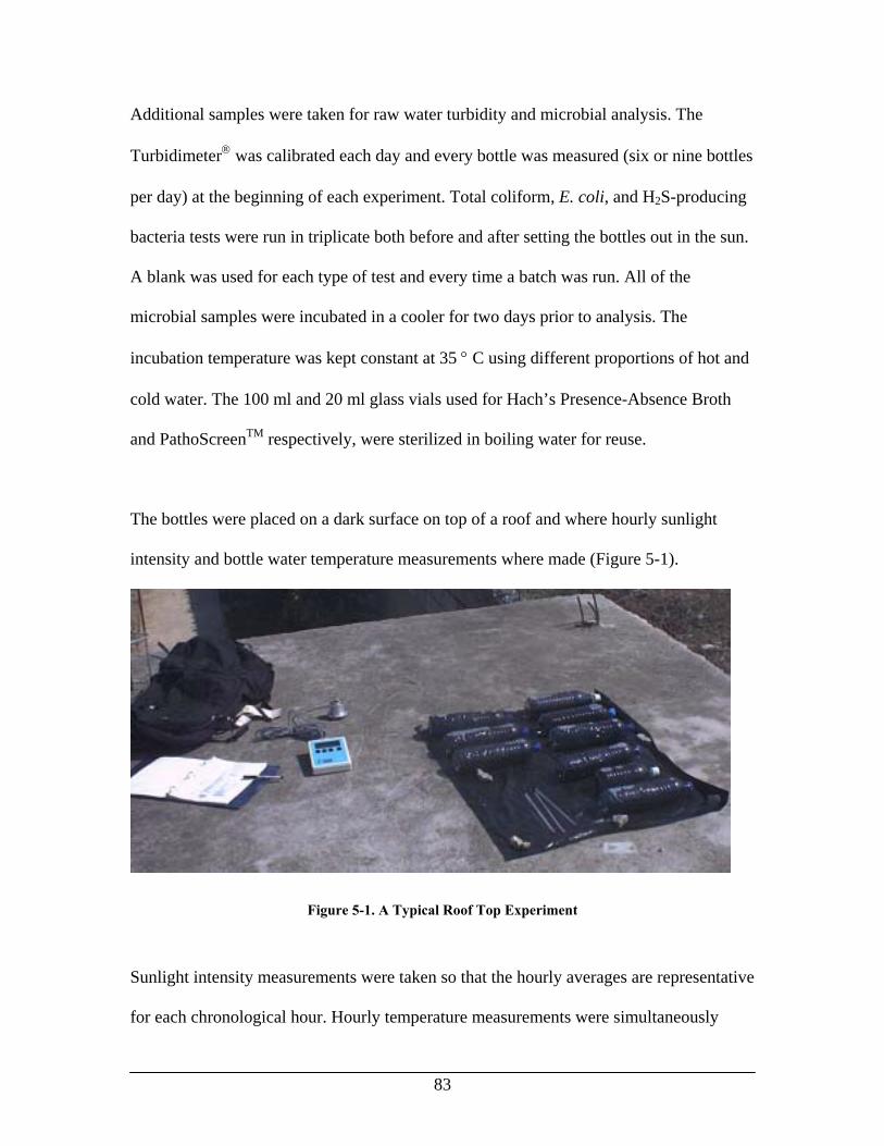
83
Additional samples were taken for raw water turbidity and microbial analysis. The
Turbidimeter was calibrated each day and every bottle was measured (six or nine bottles
per day) at the beginning of each experiment. Total coliform, E. coli, and H2S-producing
bacteria tests were run in triplicate both before and after setting the bottles out in the sun.
A blank was used for each type of test and every time a batch was run. All of the
microbial samples were incubated in a cooler for two days prior to analysis. The
incubation temperature was kept constant at 35 ° C using different proportions of hot and
cold water. The 100 ml and 20 ml glass vials used for Hach’s Presence-Absence Broth
and PathoScreenTM respectively, were sterilized in boiling water for reuse.
The bottles were placed on a dark surface on top of a roof and where hourly sunlight
intensity and bottle water temperature measurements where made (Figure 5-1).
Figure 5-1. A Typical Roof Top Experiment
Sunlight intensity measurements were taken so that the hourly averages are representative
for each chronological hour. Hourly temperature measurements were simultaneously

84
made on three bottles and the thermometers were allowed to equilibrate with the bottle
water temperature before readings were made. Most of the nights were spent completing
the microbial analysis for the daily group of designated bottles. The results of these
experiments will now be examined.

85
Section IV: Results and Discussion

86
6 Daily Results and Discussion
Field Measurements were made in Dumay on January 12th and 13th, and in Santo from
January 15th to the 21st, 2001. Both Dumay and Santo are in Area 6 from Figure 3-1. For
each day, the water source, turbidity measurement, sunlight intensity profile, temperature
profile, and the corresponding microbial analysis will be presented and discussed.
6.1 Results for Water Collected on 01/12/01
Experiments were conducted on the roof of a building at the Dumay Mission for January
12th and 13th. On January 12th, water was collected from a heavily utilized local point
source (Figure 6-1).
Figure 6-1. Water Source for 01/12/01

87
This water was very clear with an average turbidity of 1.3 ± .8 NTUs. The weather was
warm and sunny with a few scattered clouds. It was 40 °C in the sun at noon and became
slightly hazy towards the afternoon. Three bottles were placed in the dark for the duration
of the experiment to serve as controls and three were placed in the sun at 10 A.M. The
sunlight intensity profile, bottle water temperature profile, and corresponding thresholds
are shown by Figure 6-2.
SODIS Profile for 01/12/01
25
30
35
40
45
50
55
10:00 AM 11:00 AM 12:00 PM 1:00 PM 2:00 PM 3:00 PM 4:00 PM
Time [hr]
Tem
pera
ture
[°C
]
0
100
200
300
400
500
600
700
800
900
Sunl
ight
Inte
nsity
[W/m
2 ]
Average SODIS Temperature Synergistic Temperature ThresholdSunlight IntensitySunlight Intensity Disinfection Threshold
Figure 6-2. Sunlight Intensity, Average SODIS Bottle Temperature, and Corresponding Disinfection Thresholds for 01/12/01
The 5-hour average peak solar intensity was 715 W/m2, which is well above the
recommended disinfection threshold of 500 W/m2 for 5 hours. The total amount of energy
received from 10:00 A.M. to 5:00 P.M. was 4013 Wh/m2. Bottle water temperatures
surpassed the threshold of 45° C for 5 hours, indicating there would be synergistic
thermal effects. These results suggest that conditions should be excellent for SODIS. The

88
corresponding microbial analysis for the raw, dark, and SODIS water is given by Table
6-1.
Table 6-1. Results of Microbial Analysis for Raw, Dark, and SODIS Water Collected on 01/12/01
Total Coliform E. coli PathoScreenTM Sample Type
Sample Number
Raw Raw 1 √ √ √ Raw 2 √ √ √ Raw 3 √ √ √
Dark 1D √ √ √ 2D √ √ √ 3D √ √ √
Light 1L √ √ √ 2L √ √ √ 3L √ √ √
The raw water tested positive for total coliform, E. coli, and H2S-producing bacteria and
the dark bottles had no distinguishable difference. However, the bottles that were exposed
to the SODIS process tested negative for total coliform, E. coli, and H2S-producing
bacteria, indicating that all of the target organisms were completely inactivated by the
SODIS process. This suggests that for these types of conditions, SODIS was extremely
effective, producing a 100% kill rate for three different indicator organisms. Given the
sunlight and temperature profile, these results are consistent with the literature. To test
for possible bacterial regrowth, three 100 ml water samples were taken from the bottles
exposed to the SODIS process to be reanalyzed on the final day.

89
6.2 Results for Water Collected on 01/13/01
Water was collected from an on-site spring well in Dumay (Figure 6-3).
Figure 6-3. On-Site water source for 01/13/01
This water had a low turbidity of 1.2 ± .6 NTUs. Three bottles were placed in the dark
and three in the sun at 8 A.M. The morning was overcast with some haze, and black
thunderclouds moved in around 11:30. The temperature was 28° C at noon and the sky
cleared around 1:00 P.M. for an hour. Afterwards, it became cloudy again to produce a
fluctuating sunshine and temperature profile shown by Figure 6-4.

90
SODIS Profile for 01/13/01
25
30
35
40
45
50
8:00 AM 9:00 AM 10:00 AM 11:00 AM 12:00 PM 1:00 PM 2:00 PM 3:00 PM 4:00 PM 5:00 PM
Time [hr]
Tem
pera
ture
[°C
]
0
100
200
300
400
500
600
700
800
Sunl
ight
Inte
nsity
[W/m
2 ]
Average SODIS Temperature Synergistic Temperature ThresholdSunlight IntensitySunlight Disinfection Threshold
Figure 6-4. Sunlight Intensity, Average SODIS Bottle Temperature, and Corresponding Disinfection Thresholds for 01/13/01
The 5-hour average peak intensity was 530 W/m2, and the total amount of energy
measured from 8:00 A.M. to 5:00 P.M. was 3250 Wh/m2. However, the 5-hour average
peak intensity was largely raised because of the break through of sunshine around 1:00
P.M., and there were only 2 hours of sunlight intensity in excess of 500 W/m2. The bottle
water temperature never reached the synergistic threshold and these conditions are not
considered favorable for SODIS. The resulting microbial analysis is given by Table 6-2.

91
Table 6-2. Results of Microbial Analysis for 01/13/01
Total Coliform E. coli PathoScreenTM Sample Type
Sample Number
Raw Raw 1 √ √ √ Raw 2 √ √ √ Raw 3 √ √ √
Dark 1D √ √ √ 2D √ √ √ 3D √ √ √
Light 1L √ √ √ 2L √ √ √ 3L √ √ √
Every sample tested positive for all target organisms. The sunlight intensity never
reached 500 W/m2 for duration of 5 hours and the water temperature stayed below
synergistic temperature threshold. Therefore, not all of the indicator organisms were
inactivated for the bottles subjected to 1-day of the SODIS process. This implies that two
consecutive days of exposure may be required for complete disinfection. Based on these
results, the experimental methodology was shifted to incorporate the effects of 2-day
exposure (as described in section 5-1). Dark bottle controls again agreed with the raw
samples. Wegelin et al. (1994) found that the population of bacteria did not decrease in
dark bottles during the course of the experiment. Consequently, these bottles, with an
additional three, were used to investigate 2-day exposure. Furthermore, SODIS bottles
were then placed on black plastic and tire pieces to help enhance thermal effects.

92
6.3 Results for Water Collected on 01/15/01
The previous day was spent packing lab equipment and moving to Santo. The tap water at
this location was rumored to be undrinkable because of microbial contamination and was
therefore put to the SODIS test. Turbidity was very low at 1.7 ± .6 NTUs. This water was
extremely hard and produced a large amount of precipitate when boiled. The sky was
covered with heavy black thunderclouds for almost the entire day, with a special guest
appearance of the sun at around 11:00 A.M. When asked if this level of sunlight was
typical, a Haitian villager responded, “No, never this dark” (Personal communication,
01/05/01). It was 27 °C at noon, and the following sunlight and temperature profile was
observed (Figure 6-5).
SODIS Profile for 01/15/01
25
30
35
40
45
50
8:00 AM 9:00 AM 10:00 AM 11:00 AM 12:00 PM 1:00 PM 2:00 PM 3:00 PM 4:00 PM 5:00 PM
Time [hr]
Tem
pera
ture
[°C
]
0
100
200
300
400
500
600
700
Sunl
ight
Inte
nsity
[W/m
2 ]Average SODIS Temperature Synergistic Temperature ThresholdSunlight IntensitySunlight Disinfection Threshold
Figure 6-5. Sunlight Intensity, Average SODIS Bottle Temperature, and Corresponding Disinfection Thresholds for 01/15/01

93
The 5-hour average peak intensity was 383 W/m2, and the total amount of energy
measured from 8:00 A.M. to 5:00 P.M. was 2666 Wh/m2. The bottle water temperature
never reached the synergistic temperature and these conditions are poor for SODIS. The
microbial analysis is given by Table 6-3. The results of the 2-day exposure are given with
the results for the following day, as that day’s sunlight and temperature conditions have
an important influence on the outcome.
Table 6-3. Results of Microbial Analysis for 1-Day Exposure of Water Collected on 01/15/01
Total Coliform E. coli PathoScreenTM Sample Type
Sample Number
Raw Raw 1 √ √ √ Raw 2 √ √ √ Raw 3 √ √ √
1-Day 1 √ √ √ 2 √ √ √ 3 √ √ √
The raw water samples had relatively low bacterial concentrations. This was qualitatively
deduced by observing that it took almost two full days of incubation to produce a small
color change, and that two of the raw samples were negative for E. coli. This source was
not be used again because of its low level of contamination. Regardless, the SODIS
process was not 100% effective in destroying all of the tested organisms. This is in
agreement with the results for 1/13/01, which had similar sunshine and temperature
conditions. I suspect that if the raw water had higher bacterial concentrations, all of the
samples would have tested positive because of the low sunshine and temperature levels.

94
6.4 Results for Water Collected on 01/16/01
Water was collected from a local spring well in Santo very similar to Figure 6-3. The
water had a low turbidity of 1.1 ± .4 NTUs. The weather was hot and sunny with a few
scattered clouds, and the noontime temperature was 40° C in the sun. The observed
sunshine and temperature profile is given by Figure 6-6.
SODIS Profile for 01/16/01
25
30
35
40
45
50
55
8:00 AM 9:00 AM 10:00 AM 11:00 AM 12:00 PM 1:00 PM 2:00 PM 3:00 PM 4:00 PM 5:00 PM
Time [hr]
Tem
pera
ture
[°C
]
0
100
200
300
400
500
600
700
800
900
Sunl
ight
Inte
nsity
[W/m
2 ]
Average SODIS Temperature Synergistic Temperature ThresholdSunlight IntensitySunlight Disinfection Threshold
Figure 6-6. Sunlight Intensity, Average SODIS Bottle Temperature, and Corresponding Disinfection Thresholds for 01/16/01
The 5-hour average peak intensity was 710 W/m2, and the total amount of energy
received from 8:00 A.M. to 5:00 P.M. was 4920 Wh/m2. The bottle water temperature
surpassed the synergistic temperature for 4 hours and these conditions are considered
very favorable for SODIS. The microbial analysis is given by Table 6-4.

95
Table 6-4. Results of Microbial Analysis for 1-Day Exposure of Water Collected on 01/16/01 and 2-Day Exposure of Water Collected on 01/15/01
Total Coliform E. coli PathoScreenTM
Sample Type
Sample Numbe
r Raw Raw 1 √ √ √ Raw 2 √ √ √ Raw 3 √ √ √
1-Day 1 √ √ √ 2 √ √ √ 3 √ √ √ 2-Day 1-A √ √ √ (01/15/01)
1-B √ √ √
1-C √ √ √
The disinfection parameters were met and all of the target organisms were inactivated by
the SODIS process. Conclusions on the effects of 2-day exposure could not be made as
1-day exposure for 01/15/01 could have inactivated all of the organisms. However, 2-day
exposure did have 100% inactivation as expected.
6.5 Results for Water Collected on 01/17/01
To simulate scenarios when Haitians would not have access to a designated potable water
source, water with high bacterial concentrations was sought out. A puddle found by the
side of the road was chosen and named “the festering pit” (Figure 6-7). Personal
communication revealed that Haitians would never directly use a source such as “the
festering pit” for potable water. However, I was told situations could arise when they

96
would take water of this quality and try to filter it. A Gift of Water Filter, (Figure 6-8),
was used without chlorine to reduce the turbidity from 153 ± 6 NTUs to 23 ± 1.3 NTUs
before being put to the SODIS test. For more information of the Gift of Water Filter, refer
to Lantagne, 2001 and van Zyl, 2001.
Figure 6-7. "The Festering Pit" water source for 01/17/01

97
Figure 6-8. Gift of Water Filter
Raw water samples were taken after “the festering pit” water had passed through the filter
to ensure no residual chlorine in the filter bucket would kill the bacteria. The day was hot
and sunny with a noontime temperature of 38° C. Figure 6-9 shows the daily sunshine
and temperature profile.
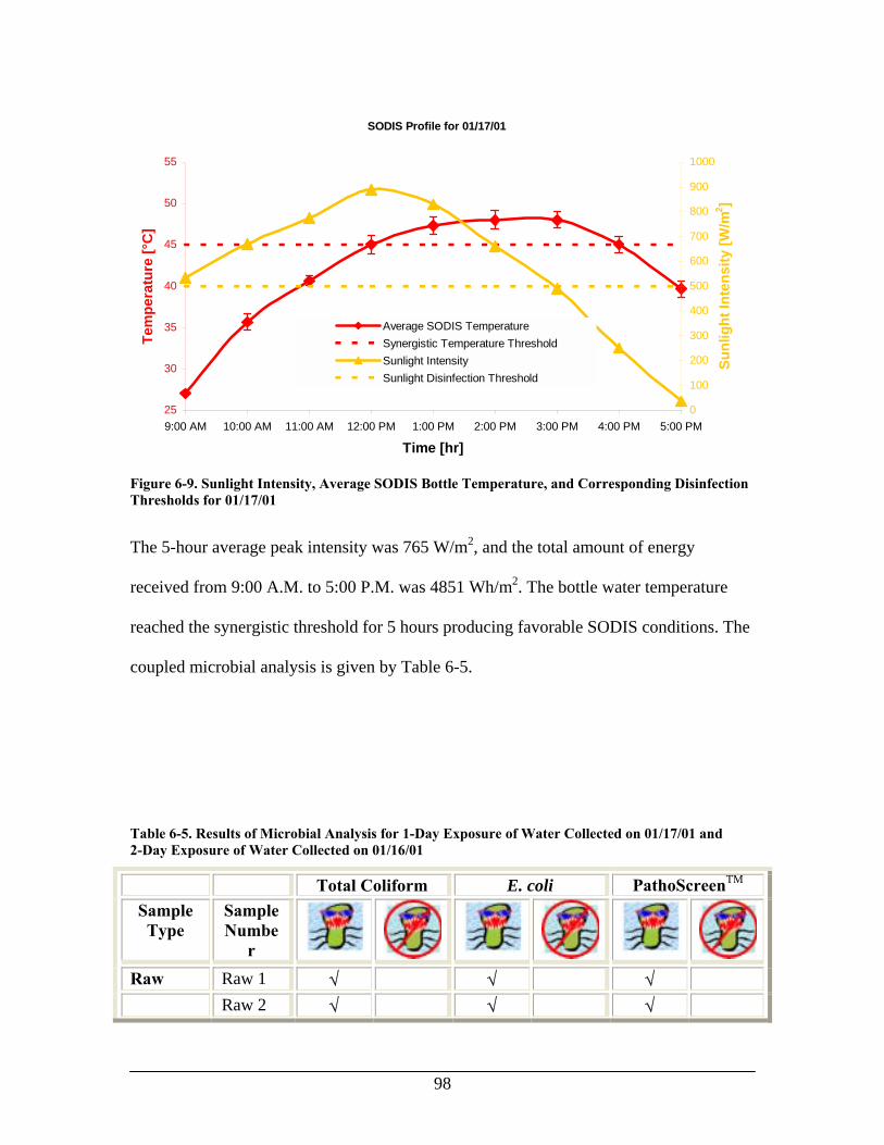
98
SODIS Profile for 01/17/01
25
30
35
40
45
50
55
9:00 AM 10:00 AM 11:00 AM 12:00 PM 1:00 PM 2:00 PM 3:00 PM 4:00 PM 5:00 PM
Time [hr]
Tem
pera
ture
[°C
]
0
100
200
300
400
500
600
700
800
900
1000
Sunl
ight
Inte
nsity
[W/m
2 ]
Average SODIS Temperature Synergistic Temperature ThresholdSunlight IntensitySunlight Disinfection Threshold
Figure 6-9. Sunlight Intensity, Average SODIS Bottle Temperature, and Corresponding Disinfection Thresholds for 01/17/01
The 5-hour average peak intensity was 765 W/m2, and the total amount of energy
received from 9:00 A.M. to 5:00 P.M. was 4851 Wh/m2. The bottle water temperature
reached the synergistic threshold for 5 hours producing favorable SODIS conditions. The
coupled microbial analysis is given by Table 6-5.
Table 6-5. Results of Microbial Analysis for 1-Day Exposure of Water Collected on 01/17/01 and 2-Day Exposure of Water Collected on 01/16/01
Total Coliform E. coli PathoScreenTM Sample Type
Sample Numbe
r Raw Raw 1 √ √ √ Raw 2 √ √ √

99
Raw 3 √ √ √
1-Day 1 √ √ √ 2 √ √ √ 3 √ √ √ 2-Day 2-A √ √ √ (01/16/01)
2-B √ √ √
2-C √ √ √
Contrary to expectation, the raw water results turned positive at comparable rates to
previous water sources and produced similar color intensities. This suggests that the
bacterial concentrations were not as high as hoped. The sunlight and temperature
disinfection criteria was met and all the target organisms where inactivated. The effects
of 2-day exposure could not be firmly concluded because all of the organisms could have
been inactivated on 01/17/01, but the 2-day exposure still produced 100% disinfection.
6.6 Results for Water Collected on 01/18/01
After the disappointing bacterial concentrations produced by “the festering pit,” a search
was undertaken for an even stronger source. Two goats, one cow, and a little boy were
observed defecating in an irrigation stream, which was then selected for the SODIS test.
Personal communication revealed that since the installment of local spring wells, this
type of source was thankfully no longer required. The motivation for testing this type of
source is if SODIS can work on water with large numbers of bacteria and high turbidity,
it will certainly work on clearer water with lower microbial concentrations. The part of
the irrigation stream sampled is shown by Figure 6-10.

100
Figure 6-10. Local Stream water source for 01/18/01
The stream was not as clear as the more realistic water sources previously sampled, and
had a turbidity of 26 ± 3 NTUs. It had rained heavily for a brief period during the night,
and runoff could have affected the stream’s turbidity. The day was very sunny with a few
clouds in the afternoon, and was slightly windier than past days. The noontime
temperature in the sun was 37° C, and the corresponding sunlight and temperature profile
is shown by Figure 6-11.

101
SODIS Profile for 01/18/01
23
28
33
38
43
48
53
8:00 AM 9:00 AM 10:00 AM 11:00 AM 12:00 PM 1:00 PM 2:00 PM 3:00 PM 4:00 PM 5:00 PM
Time [hr]
Tem
pera
ture
[°C
]
0
100
200
300
400
500
600
700
800
900
1000
Sunl
ight
Inte
nsity
[W/m
2 ]
Average SODIS Temperature Synergistic Temperature ThresholdSunlight IntensitySunlight Disinfection Threshold
Figure 6-11. Sunlight Intensity, Average SODIS Bottle Temperature, and Corresponding Disinfection Thresholds for 01/18/01
The 5-hour average peak intensity was 768 W/m2, and the total amount of energy
received from 8:00 A.M. to 5:00 P.M. was 5265 Wh/m2. The bottle water temperature
was over the synergistic threshold for 3 hours, providing favorable SODIS conditions.
The microbial analysis for 01/18/01 is given by Table 6-6.

102
Table 6-6. Results of Microbial Analysis for 1-Day Exposure of Water Collected on 01/18/01 and 2-Day Exposure of Water Collected on 01/17/01
Total Coliform E. coli PathoScreenTM Sample
Type Sample Number
Raw Raw 1 √ √ √ Raw 2 √ √ √ Raw 3 √ √ √
1-Day 1 √ √ √ 2 √ √ √ 3 √ √ √
2-Day 1-A √ √ √ (01/17/01) 1-B √ √ √ 1-C √ √ √
The raw water samples produced extremely strong positives in approximately 4 hours.
The H2S test turned so black, that the black ink labels on the bottle where no longer
legible without first emptying the contents of the bottle. Furthermore, the coliform
bacteria built up enough pressure by gas production, that the 100 ml bottles exploded
almost their entire contents when opened. After my first shower, the remaining bottles
were opened inside a garbage bag. This confirmed that the irrigation stream indeed had
high bacterial concentrations. In fact, despite the favorable SODIS conditions of over 7
hours of sunshine in excess of 500 W/m2, a 5-hour average peak intensity was 768 W/m2,
and 3 hours above the synergistic temperature, almost all of the 1-day samples still gave
weak positive results. This result is attributed to the high initial amount of bacteria
present. The 2-day samples from 01/17/01 were all negative but the microbes could have
easily been completely inactivated on either day. It was also observed that the water
temperatures seemed slightly low, given the amount of sunshine received. This could be

103
because the initial temperature was slightly colder than normal at 23 °C compared to the
typical 26 °C. Additionally, the slight increase in wind could have caused some
convective cooling effects.
6.7 Results for Water Collected on 01/19/01
Water was again collected from the irrigation stream because of its high bacterial
concentrations. The turbidity was much lower than the previous day at 7 ± .8 NTUs,
which could be explained by the lack of rain. The day was mostly sunny with a few
scattered clouds and it was very windy. A noontime air temperature of 38 °C was
observed, and the day’s sunshine and temperature profile is given by Figure 6-12.
SODIS Profile for 01/18/01
25
30
35
40
45
50
8:00 AM 9:00 AM 10:00 AM 11:00 AM 12:00 PM 1:00 PM 2:00 PM 3:00 PM 4:00 PM 5:00 PM
Time [hr]
Tem
pera
ture
[°C
]
0
100
200
300
400
500
600
700
800
900
Sunl
ight
Inte
nsity
[W/m
2 ]Average SODIS Temperature Synergistic Temperature ThresholdSunlight IntensitySunlight Disinfection Threshold
Figure 6-12. Sunlight Intensity, Average SODIS Bottle Temperature, and Corresponding Disinfection Thresholds for 01/19/01

104
The 5-hour average peak intensity was 761 W/m2, and the total amount of energy
received from 8:00 A.M. to 5:00 P.M. was 5330 Wh/m2. The bottle water temperature
never surpassed the synergistic threshold despite the large amount of sunshine and fairly
warm ambient temperatures. The microbial analysis is given by Table 6-4.
Table 6-7. Results of Microbial Analysis for 1-Day Exposure of Water Collected on 01/19/01 and 2-Day Exposure of Water Collected on 01/18/01
Total Coliform E. coli PathoScreenTM
Sample Type
Sample Number
Raw Raw 1 √ √ √ Raw 2 √ √ √ Raw 3 √ √ √
1-Day 1 √ √ √ 2 √ √ √ 3 √ √ √
2-Day 2-A √ √ √ (01/18/01) 2-B √ √ √ 2-C √ √ √
The raw water samples again exhibited the same strong positives as they did on 01/18/01.
This day received 7 hours of sunshine over the recommended threshold and had a
relatively high 5-hour average peak intensity. However, two-thirds of the samples tested
weakly positive for all of the target organisms. This is most likely a result of the high
initial amount of bacteria and the fact that the bottles never reached the synergistic
temperature threshold. Bottle temperatures were probably suppressed by the convective
cooling effects of this day’s strong wind. An important result is that the 2-day samples all

105
tested negative, while the samples from 1-day exposure for both days still had target
bacteria present. This clearly shows that 2 days of exposure produce superior bacterial
inactivation when compared to 1 day of the SODIS process.
6.8 Results for Water Collected on 01/20/01
Water was collected for the last time at the irrigation stream. The water had a turbidity of
13.2 ± 3.8 NTUs. The day was partly cloudy and the temperature in the sun was 38 °C at
noon. High winds were again observed. This time a board was placed near the bottles to
shelter them from any convective cooling effects, but not so close that it would cast a
shadow on the bottles. The sunlight and temperature profile is shown by Figure 6-13.
SODIS Profile for 01/20/01
25
30
35
40
45
50
8:00 AM 9:00 AM 10:00 AM 11:00 AM 12:00 PM 1:00 PM 2:00 PM 3:00 PM 4:00 PM 5:00 PM
Time [hr]
Tem
pera
ture
[°C
]
0
100
200
300
400
500
600
700
800
900
Sunl
ight
Inte
nsity
[W/m
2 ]
Average SODIS Temperature
Synergistic Temperature Threshold
Sunlight IntensitySunlight Disinfection Threshold
Figure 6-13. Sunlight Intensity, Average SODIS Bottle Temperature, and Corresponding Disinfection Thresholds for 01/20/01

106
The 5-hour average peak intensity was 729 W/m2, and the total amount of energy
received from 8:00 A.M. to 5:00 P.M. was 4742 Wh/m2. The bottle water temperature
surpassed the synergistic temperature for 4 hours. An important observation is that the
bottle temperatures did reach the synergistic temperature threshold for over 4 hours
despite having strong winds similar to the previous day. Furthermore, this day had a
lower 5-hour average peak intensity, 729 W/m2, than on 01/19/01, 761 W/m2.
Comparatively between these two days, the ambient temperatures were about the same,
01/20/01 received less sunshine, and 01/20/01 had higher bottle water temperatures
because of the difference in wind. This suggests that blocking convective cooling may be
an important aspect of SODIS in windy conditions. The microbial analysis for 01/20/01 is
given by Table 6-8.
Table 6-8. Results of Microbial Analysis for 1-Day Exposure of Water Collected on 01/20/01 and 2-Day Exposure of Water Collected on 01/19/01
Total Coliform E. coli PathoScreenTM Sample
Type Sample Number
Raw Raw 1 √ √ √ Raw 2 √ √ √ Raw 3 √ √ √
1-Day 1 √ √ √ 2 √ √ √ 3 √ √ √
2-Day 1-A √ √ √ (01/19/01) 1-B √ √ √ 1-C √ √ √

107
The raw water had the same high concentrations of bacteria as described on 01/18/01.
Favorable conditions were once again dwarfed by the high initial concentrations of
bacteria and two-thirds of the 1-day samples tested weakly positive for all the target
organisms. The 2-day exposure again had a 100% kill rate while the 1-day exposures
achieved only 66% inactivation.
6.9 Results for 01/21/01
The 2-day bottles from 01/20/01 were placed outside again on 01/21/01. The day started
out very sunny but heavy clouds appeared for an hour around 1:00 P.M. The noontime
temperature was 38 °C in the sun. The following sunlight and temperature profile was
produced (Figure 6-14).
SODIS Profile for 01/21/01
25
30
35
40
45
50
8:00 AM 9:00 AM 10:00 AM 11:00 AM 12:00 PM 1:00 PM 2:00 PM 3:00 PM 4:00 PM 5:00 PM
Time [hr]
Tem
pera
ture
[°C
]
0
100
200
300
400
500
600
700
800
900
Sunl
ight
Inte
nsity
[W/m
2 ]
Average SODIS Temperature Synergistic Temperature ThresholdSunlight IntensitySunlight Disinfection Threshold
Figure 6-14. Sunlight Intensity, Average SODIS Bottle Temperature, and Corresponding Disinfection Thresholds for 01/21/01

108
The 5-hour average peak intensity was 664 W/m2, and the total amount of energy
received from 8:00 A.M. to 5:00 P.M. was 4509 Wh/m2. The bottle water temperature
reached the synergistic temperature for 2-nonconsecutive hours. The microbial analysis
of the bottles testing for bacterial regrowth from 01/12/01 is also given by Table 6-9.
Table 6-9. Results of Microbial Analysis 2-Day Exposure of Water Collected on 01/19/01 and for Bacterial Regrowth from water on 01/12/01
Total Coliform E. coli PathoScreenTM Sample
Type Sample Number
2-Day 2-A √ √ NA NA (01/20/01) 2-B √ √ √ 2-C √ √ √ Regrowth 1 √ √ √ (01/12/01) 2 √ √ √ 3 √ √ √
Consistent with previous 2-day exposures, 100% inactivation was achieved. Sample
2-Day2-A for the H2S-producing bacteria was disregarded, as the cap for the 20 ml vial
was broken. No bacterial regrowth was observed for any of the target organisms, which is
consistent with the results found by Wegelin (1994).
7 Summary of Results and Discussion
The general results for turbidity, sunlight intensity, how the measured and modeled
sunlight intensity compared, and the overall microbial analysis will be presented. These
results and what they imply for SODIS in Haiti will then be discussed.

109
7.1 Summary of Results
7.1.1 Turbidity
All realistic water sources were very clear with an average turbidity of 1.3 ± .6 NTUs.
This is consistent with Lantagne (2001), who found an average turbidity of .88 ± .84
NTUs collected from several other places in Haiti.
7.1.2 Sunshine and Temperature
The average sunshine intensity and temperature profile for all days, January 12th through
January 21st, 2001 is given by Figure 7-1.
Overall Average Sunlight and Temperature Profiles
25
30
35
40
45
50
55
8:00 AM 9:00 AM 10:00 AM 11:00 AM 12:00 PM 1:00 PM 2:00 PM 3:00 PM 4:00 PM 5:00 PM
Time [hours]
Tem
pera
ture
[°C
]
0
100
200
300
400
500
600
700
800
900
1000
Sunl
ight
Inte
nsity
[W/m
2 ]
Average SODIS Temperature Synergistic Temperature ThresholdSunlight IntensitySunlight Disinfection Threshold
Figure 7-1. Average Sunlight and Bottle Water Temperature observed in Haiti during January

110
The 5-hour average peak intensity was 651 W/m2, and the average total amount of daily
energy received was 4537 Wh/m2. On average, the bottle water temperature hovered
around the synergistic temperature for about 3 hours.
Two of the nine days were under the cover of thunderclouds and had sunlight and
temperature profile shown by Figure 7-2.
Average Cloudy Profile
25
30
35
40
45
50
8:00 AM 9:00 AM 10:00 AM 11:00 AM 12:00 PM 1:00 PM 2:00 PM 3:00 PM 4:00 PM 5:00 PM
Time [hr]
Tem
pera
ture
[°C
]
0
100
200
300
400
500
600
700
800
Sunl
ight
Inte
nsity
[W/m
2 ]
Average SODIS Temperature Synergistic Temperature ThresholdSunlight IntensitySunlight Disinfection Threshold
Figure 7-2. Average Stormy Day Profile Observed for the 13th and 15th of January (2 of 9 days)
For these two stormy days, the 5-hour average peak intensity was 445 W/m2, and the total
amount of energy received was 2958 Wh/m2. The bottle water temperature never reached
the synergistic threshold.

111
Subtracting these two stormy days from the rest paints a better picture of a typical day of
Haitian sunshine and bottle water temperature. This can be seen in Figure 7-3 by the
decrease in the size of the error bars when compared to Figures 7-1 and 7-2.
Average Sunny Profile
25
30
35
40
45
50
55
8:00 AM 9:00 AM 10:00 AM 11:00 AM 12:00 PM 1:00 PM 2:00 PM 3:00 PM 4:00 PM 5:00 PM
Time [hr]
Tem
pera
ture
[°C
]
0
100
200
300
400
500
600
700
800
900
1000
Sunl
ight
Inte
nsity
[W/m
2 ]
Average SODIS Temperature Synergistic Temperature ThresholdSunlight IntensitySunlight Disinfection Threshold
Figure 7-3. Average Non-Stormy Day Profile for Partly Cloudy to Mostly Sunny days (7 of 9).
For the average of the non-stormy days, the 5-hour average peak intensity was 735 W/m2,
and the total amount of energy received was 5061Wh/m2. The bottle water temperature
rose past the synergistic threshold for 4 hours.
7.1.3 Measured Intensity Comparison to Model Prediction
The sunlight intensity measurements were made in Area 6 from Figure 3-1. The
measured average, minimum, and maximum 5-hour peak intensity values will be
compared to the simulated values in January for Area 6 (Table 7-1).

112
Table 7-1. Comparison between Simulated and Observed Average, Minimum, and Maximum 5-hour Average Peak Intensity Values.
Simulated (W/m2) Observed (W/m2) Percent Agreement Average 641 651 98.5 % Minimum 615 383 62.3 % Maximum 660 768 86.0 %
The simulated and measured average values are in excellent agreement. However, the
maximum and minimum are significantly different. The reason for this disagreement
becomes apparent when looking at the measured minimum and maximum daily total
energies compared to the 10-year average values obtained from NASA. The measured
minimum day had a measured total energy value of 2666 Wh/m2. This value was roughly
adjusted to 2800 Wh/m2 to compensate for the period between 6:00 A.M. and 8:00 A.M
when there was sunshine but no measurements. Similarly, the maximum intensity was
adjusted from 5265 Wh/m2 to 5600 Wh/m2 to compensate for the missed sunlight
between 6:00 A.M. to 8:00 A.M. A comparison of percent agreement between the two
total energy values along with the intensity values is given by Table 7-2.
Table 7-2. Percent Agreement between Simulated and Observed Intensity Values, and Observed and NASA 10-year Average Total Energy Values for the Maximum and Minimum Energy in January
Simulated (W/m2)
Observed (W/m2)
Intensity Percent
Agreement
Observed Total Energy
(Wh/m2)
Total Energy Provided by
NASA (Wh/m2)
Total Energy Percent
Agreement Minimum 615 383 62.3 % 2800 4490 62.4 % Maximum 660 768 86.0 % 5600 4960 88.6 %
The difference in total energy adequately explains the difference in intensity because they
are so intimately related. To verify this, the observed minimum total energy value is
plugged into the model and it produces a 5-hour average peak intensity value of 385

113
W/m2. This minimum average intensity is in over 99% agreement with the observed
value of 383 W/m2. The maximum observed value produces a 5-hour average peak
intensity of 770 W/m2, which is in over 99% agreement with the observed maximum
value of 768 W/m2. It then follows that the discrepancy between the simulated and
observed minimum and maximum results can be explained by the total energy values
provided by NASA. The reported minimum and maximum NASA total energies are
likely different from the measured values because they are representative of a 10-year
average for a degree latitude and longitude quantity. However, the measured amounts are
at a much smaller scale within that averaged area making them more susceptible to local
fluctuations.
7.1.4 Overall Microbial Analysis
Microbial testing was conducted using total coliform, E. coli, and H2S-producing bacteria
to assess how SODIS performed under various conditions. The total results for the raw
water, 1-day exposure, and 2-day exposure are given by Table 7-3.
Table 7-3. Overall Microbial Analysis
Initial Raw Contamination %, (Positive/Sampled)
1-Day Kill %, (Negative/Sampled)
2-Day Kill %, (Negative/Sampled)
97.2%, (70/72) 52.8%, (38/72) 100%, (53/53)
The three types of microbial tests showed good agreement between one another for both
positive and negative results for all tests made (Table 7-4).

114
Table 7-4. Percent Agreement between Different Microbial Tests
Type of Agreement Total Coliform and E. coli
Total Coliform and H2S Bacteria
E. coli and H2S Bacteria
Positive 92.7 % 95.1 % 97.4 % Negative 91.2 % 96.9 % 94.1 %
The different tests were in strong agreement indicating the raw water had all of the target
organisms present and that the SODIS process had roughly the same effect on the
different types of indicator bacteria.
7.2 Discussion
Every point source that people used for potable water in Dumay and Santo had very low
turbidity. Lantagne (2001) sampled several other locations in Haiti to find that they all
had minimal turbidity. Based on the measurements made in January, it would be
reasonable to say that most places would not need a prefiltration step and SODIS could
be directly applied. However, to make a broader conclusion, additional samples would
have to be taken in the rainy seasons (around October and May) to investigate how
increased runoff would affect turbidity.
The intense Haitian sunshine and warm climate appear to provide conditions suitable for
effective SODIS. This research was conducted during Haiti’s winter, implying shorter
and colder days compared to most of the year. However, “the rainy months like October
and May, could receive less sunshine, but you could easily count the days on your fingers
in Haiti that receive no sunshine because they are so few” (Nathan Dieudonne, personal
communication, 1/14/01). It would be important to conduct further SODIS testing around

115
October when there is less sunshine and increased cloudiness. The highly heterogeneous
nature of Haiti’s climate makes general conclusions difficult to formulate. At higher
altitudes, the orographic enhanced cloud cover and the colder temperatures could
compromise the effectiveness of SODIS. If the mountainous regions are too cold to
realistically incorporate synergistic thermal effects, the bottles should not be painted
black and could be placed in solar reflectors. This would have the SODIS process rely
solely on optical inactivation, which could be very effective given there is more UV
radiation at higher altitudes. If this technique were ineffective, an alternative disinfection
method would have to be used in the mountainous regions.
The mathematical sunshine model proved to be very accurate in predicting the 5-hour
average peak sunshine intensity for a given total energy value. However, caution should
be used when applying the NASA values obtained for the 10-year average of the average,
minimum, and maximum total daily energy. The average monthly values are regarded as
more accurate because they sample around 30 or 31 days per month, and that average is
then averaged over the span of 10 years. However, measurements for the minimum and
maximum energies are a single value for each month, and their average comes from a
much smaller sample population. More importantly, the NASA values are assumed
accurate for what they represent, but their spatial resolution does not capture the presence
of microclimates within a degree longitude and latitude. This can cause inaccurate
predictions for specific locations within highly heterogeneous areas smaller than a degree
longitude and latitude. However, simulated values would likely be much more accurate
for specific locations in a homogeneous site. The mathematical model that was presented
is a valuable tool to obtain a first approximation if SODIS would be applicable for Haiti

116
throughout the year. This method of sunshine simulation could easily be applied to
estimate the year-round SODIS effectiveness anywhere else in the world. One would
only need to obtain the locations latitude and total energy values from a source such as
NASA. If the sunlight intensities appear adequate for a location, then physical tests
should be conducted to evaluate the success of SODIS.
SODIS efficacy was evaluated by the inactivation of total coliform, E. coli, and
H2S-producing bacteria. The results verify that Haiti does have water problems with
microbial contamination as 97% of the samples tested positive for all indicator
organisms. Impacts of exposure duration varied significantly between 1-day and 2-day
periods. Under various sunshine intensities, bottle water temperatures, and initial
bacterial concentrations, 1-day exposure completely inactivated all of the bacteria half of
the time, while the 2-day exposure period achieved 100% inactivation for all conditions
experienced. A major drawback of this study is two consecutive stormy days such as on
01/15/01 were not observed and SODIS efficacy for these conditions in Haiti is unknown.
Guidelines that differentiate between 1-day and 2-day exposure have been suggested in
the literature. However, it is considered more practical to have every bottle exposed for a
2-day duration. It was observed that 100% bacteriological inactivation is mainly a
function on sunlight, temperature, and initial microbial concentration (the effects of
turbidity and wind are considered less important for Haiti). These parameters are highly
variable and the right conditions for 100% inactivation with 1-day exposure were only
met half of the time. To ask a villager to gauge how much sunshine a specific day has

117
received takes away from the simplistic beauty of this technology. First, it is distracting
for villagers to have to constantly think about how much sunshine a bottle is receiving.
Second, this judgment is prone to large errors (I met a man who told me he was 177 years
old), which could ultimately cause illness or death. If the 2-day exposure results that were
observed in January hold true, leaving every bottle out in the sun for 2-day exposure
would take the guess work out of this technology and would always lean towards the
conservative side of disinfection. A practical way of providing people with cold water
every morning that has undergone a 2-day exposure period can be termed “a SODIS
triangle.” Essentially, it consists of three groups of bottles that are rotated every morning,
so two groups are out in the sun and one is being used for consumption. This process is
illustrated in detail in the next section. From the experiences and the results produced in
Haiti, a set of practical application guidelines has been constructed.

118
Section V: Practical Application Guidelines

119
The SODIS disinfection process is simple to apply but would require training at the
community level to ensure optimal benefits. These guidelines are a product of what was
experienced in Haiti along with some adaptations from the SODIS Technical Notes
(EAWAG/SANDEC), and should be applied to those areas deemed suitable for SODIS.
8 Practical SODIS Procedure
8.1 Bottles
Collect Clear PET bottles from home or local market of 1-2 liters. Enough should be obtained to sustain a household level of consumption. PET bottles can be easily identified as they will say PET on the bottom or they main contain the following symbol:
Make sure the bottles are not to scratched up so light can easily penetrate.
Make sure the bottles do not leak and have caps that seal watertight.
All labels should be removed and both the inside and outside of the bottles should be washed to ensure optimal light transmittance.
Paint half of the bottles black (if paint is available): • The side with any residual label glue should be painted. This
eliminates the hassle of trying to remove it and prevents future dirt build up, which would reduce light transmittance.
• Use as many paint coats as necessary to create an opaque finish. • Hold the bottle up to light and make sure light does not come through
the bottom.

120
8.2 Water
Water should be obtained from a common village supply: well, stream, pond, reservoir, etc.
Water must be clear enough for SODIS to work. Turbidity can be checked by placing a copy of the SODIS logo under the bottle and checking its readability.
If the logo is legible, then turbidity is low enough for SODIS. If not, the
water must be left to settle or processed with a filter if available.
When collecting water, rinse the outside of the bottle to remove any buildup that would block sunlight transmission
Fill the SODIS bottles about two-thirds full and screw on the cap. Shake the bottles vigorously for about 20 seconds to ensure the water is sufficiently oxygenated. The bottles are now ready for exposure.
Place logo under a bottle Put in sun (<30 NTUs) Have to filter or let settle until logo is legible (>30 NTUs)

121
8.3 Exposure
An area must be chosen that receives sunshine throughout the entire day.
Place bottles on dark surfaces to enhance thermal inactivation such as black plastic or tire pieces, which appear to be ubiquitous in Haitian garbage. Corrugated metal rooftops reach high temperatures and they would be excellent SODIS areas if they receive full sunshine during the day.
Bottles should be sheltered from high winds, if the occasion calls for it, to decrease thermal depletion by convection (wind blowing the heat away from the bottles). Make sure that any objects use to shelter wind do not shelter sunshine.
To make things simple, routine, and conservative, groups of bottles should be set out for two days, regardless of the weather conditions. This takes out the guesswork as to the whether conditions are right for SODIS. A practical approach to this exposure guideline would be to set up a “SODIS Triangle.” This involves three groups of bottles: A, B, and C; and two designated SODIS areas: SODIS Area 1 and SODIS Area 2. The two areas could simply be adjacent spots on a roof. The SODIS Triangle is set up as follows:
Morning of Day 1:
SODIS Area 1 SODIS Area 2
A
A
• Collect water with group A • Place bottle group A in
SODIS Area 1
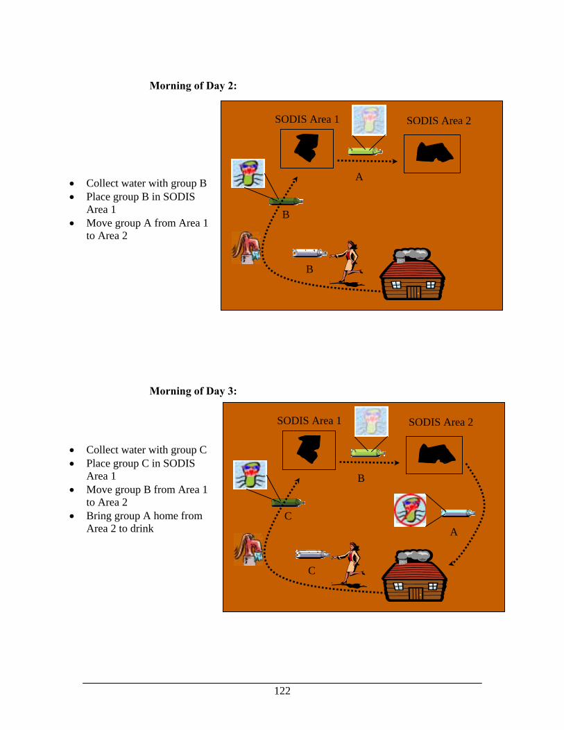
122
Morning of Day 2:
Morning of Day 3:
SODIS Area 1 SODIS Area 2
C
C
B
A
SODIS Area 1 SODIS Area 2
B
B
A• Collect water with group B • Place group B in SODIS
Area 1 • Move group A from Area 1
to Area 2
• Collect water with group C • Place group C in SODIS
Area 1 • Move group B from Area 1
to Area 2 • Bring group A home from
Area 2 to drink

123
Morning of Day 4: This now establishes an indefinite loop where a person goes out in the
morning to fill up a group of bottles and returns the same morning with a group of bottles that have undergone two days of SODIS treatment. This has the added advantage that the bottles have been allowed to cool over night.
8.4 Anticipated Mistakes
Some bottles are placed in sunny areas in the morning but the areas become shady after a few hours.
Many people like to place their bottles on chairs, but the chair backs shade bottles after a few hours.
Some users expose the bottle with the black side on top.
Users don’t plan well, become impatient, drink the water prematurely, and get sick.
SODIS Area 1 SODIS Area 2
A
A
C
B
• Collect water with group A • Place group A in SODIS
Area 1 • Move group C from Area 1
to Area 2 • Bring group B home from
Area 2 to drink

124
Section VI: Summary and Conclusions
125
9 Summary and Conclusions
SODIS is a simple technology that operates on the principle that sunlight-induced DNA
alteration, photo-oxidative destruction, and thermal effects will inactivate
microorganisms. The treatment process consists of filling plastic bottles with water and
exposing them to sunlight. Using this technique, 100% inactivation of total coliform, E.
coli, and H2S-producing bacteria was achieved after a 2-day exposure period under a
variety of conditions. Based on these results in January, it is recommended that a “SODIS
triangle” be applied to ensure every bottle receives 2 days of the SODIS process.
Mathematical sunshine simulations suggest that SODIS would be applicable, on average,
throughout Haiti year-round. However, this model does not take into account
microclimates and mountainous areas may have limited success due to lower sunshine
and temperature. This aspect needs further research. Overall, the results are encouraging
and it is strongly recommended that SODIS be further investigated for at least some parts
of Haiti. It is hoped that this extremely affordable point-of-use treatment technology can
help alleviate the water quality problems that currently plague Haiti. To evaluate SODIS
as a point-of-use treatment technology, it will be compared to the point-of-use water
treatment criteria established in section 1.4 and summarized in Table 9-1.
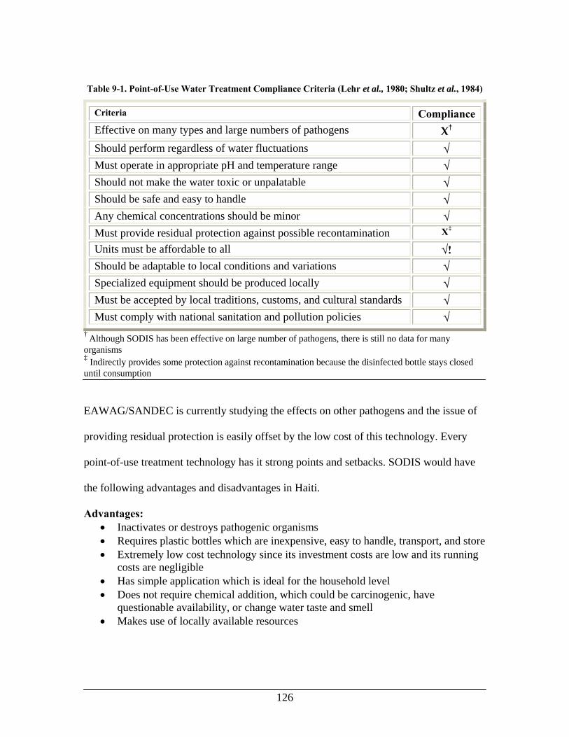
126
Table 9-1. Point-of-Use Water Treatment Compliance Criteria (Lehr et al., 1980; Shultz et al., 1984)
† Although SODIS has been effective on large number of pathogens, there is still no data for many organisms ‡ Indirectly provides some protection against recontamination because the disinfected bottle stays closed until consumption
EAWAG/SANDEC is currently studying the effects on other pathogens and the issue of
providing residual protection is easily offset by the low cost of this technology. Every
point-of-use treatment technology has it strong points and setbacks. SODIS would have
the following advantages and disadvantages in Haiti.
Advantages: • Inactivates or destroys pathogenic organisms • Requires plastic bottles which are inexpensive, easy to handle, transport, and store • Extremely low cost technology since its investment costs are low and its running
costs are negligible • Has simple application which is ideal for the household level • Does not require chemical addition, which could be carcinogenic, have
questionable availability, or change water taste and smell • Makes use of locally available resources
Criteria Compliance Effective on many types and large numbers of pathogens Χ† Should perform regardless of water fluctuations √ Must operate in appropriate pH and temperature range √ Should not make the water toxic or unpalatable √ Should be safe and easy to handle √
Any chemical concentrations should be minor √ Must provide residual protection against possible recontamination Χ‡
Units must be affordable to all √! Should be adaptable to local conditions and variations √
Specialized equipment should be produced locally √ Must be accepted by local traditions, customs, and cultural standards √ Must comply with national sanitation and pollution policies √
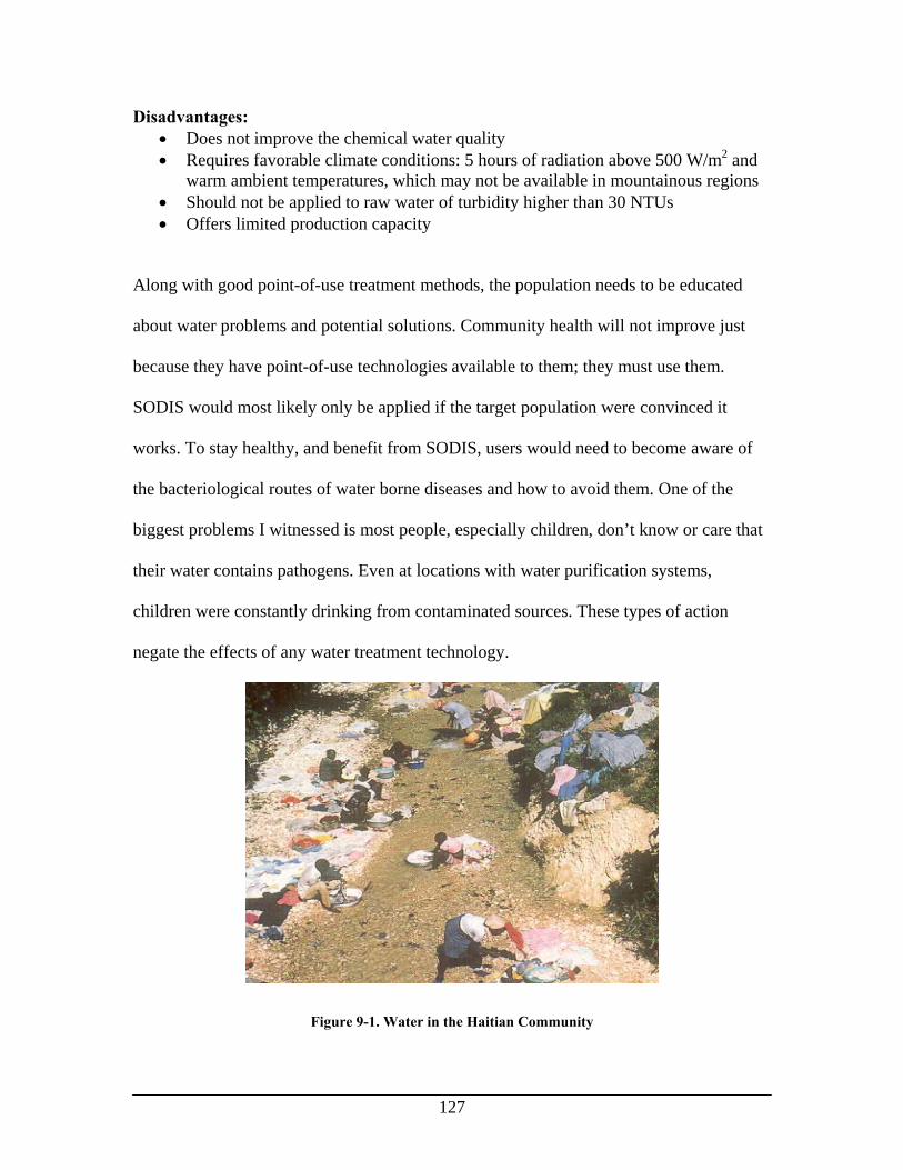
127
Disadvantages: • Does not improve the chemical water quality • Requires favorable climate conditions: 5 hours of radiation above 500 W/m2 and
warm ambient temperatures, which may not be available in mountainous regions • Should not be applied to raw water of turbidity higher than 30 NTUs • Offers limited production capacity
Along with good point-of-use treatment methods, the population needs to be educated
about water problems and potential solutions. Community health will not improve just
because they have point-of-use technologies available to them; they must use them.
SODIS would most likely only be applied if the target population were convinced it
works. To stay healthy, and benefit from SODIS, users would need to become aware of
the bacteriological routes of water borne diseases and how to avoid them. One of the
biggest problems I witnessed is most people, especially children, don’t know or care that
their water contains pathogens. Even at locations with water purification systems,
children were constantly drinking from contaminated sources. These types of action
negate the effects of any water treatment technology.
Figure 9-1. Water in the Haitian Community

128
Ultimately, this point-of-use treatment option is very attractive as it could provide a safe
source of water at the cost of a plastic bottle. It is hoped that this relatively new
disinfection method will produce an economically feasible technology to improve water
quality and public health in Haiti.

129
Appendix: Code Used for Sunlight Simulation % Numerical Model of Daily Sunlight Profile % Peter Oates % 2/24/01 % MIT %clear; clf; % Data for total Energy obtained from NASA % Set Trip = 1,2,3 for average, minimum, maximum, or 4 year respectively trip=1; % Set cal=1 if you want to run calibration plots for noon data % note: have to change the length of the n vector to average over the appropriate time cal=1; %noon time calibration data noondat1=[0.64 0.72 0.76 0.78 0.73 0.72 0.73 0.74 0.71 0.64 0.59 0.56]*1000; noondat2=[0.62 0.70 0.75 0.76 0.71 0.69 0.70 0.72 0.68 0.61 0.56 0.56]*1000; noondat3=[0.61 0.69 0.74 0.75 0.70 0.67 0.68 0.69 0.66 0.66 0.62 0.54]*1000; noondat4=[0.68 0.75 0.80 0.80 0.76 0.74 0.74 0.75 0.72 0.66 0.62 0.61]*1000; noondat5=[0.65 0.73 0.77 0.77 0.72 0.70 0.71 0.72 0.69 0.63 0.59 0.57]*1000; noondat6=[0.63 0.70 0.75 0.75 0.69 0.66 0.67 0.69 0.66 0.60 0.56 0.56]*1000; %My data for calibration dat=[0.0000 120.0000 340.7500 519.0000 666.8333 793.6667 814.0000 749.6667 650.1667 461.3333 203.3333 65.33334 0.0000]; if trip==1 %Average Data Kw/m2/day E=[4.68 5.32 5.99 6.30 6.16 5.99 5.96 5.86 5.61 4.95 4.50 4.28 %Area 1 4.59 5.23 5.89 6.16 6.03 5.80 5.79 5.70 5.46 4.84 4.42 4.21 %Area 2 4.51 5.16 5.86 6.13 5.98 5.69 5.68 5.58 5.36 4.76 4.36 4.13 %Area 3 4.90 5.52 6.21 6.47 6.26 6.09 6.01 5.91 5.72 5.08 4.66 4.51 %Area 4 4.79 5.38 6.03 6.22 6.04 5.80 5.75 5.68 5.49 4.91 4.54 4.40 %Area 5 4.68 5.25 5.89 6.04 5.86 5.54 5.52 5.47 5.29 4.76 4.44 4.30 %Area 6 4.55 5.15 5.82 5.99 5.79 5.40 5.37 5.31 5.15 4.66 4.36 4.21]; %Area 7 end if trip==2 %Minimum Data E=[4.40 5.05 5.67 5.62 5.39 5.55 5.78 5.45 5.00 4.38 3.99 3.91 %Area 1 4.36 4.96 5.56 5.58 5.35 5.42 5.59 5.32 4.88 4.29 3.92 3.79 %Area 2

130
4.34 4.87 5.52 5.54 5.31 5.36 5.48 5.23 4.91 4.13 3.90 3.70 %Area 3 4.66 5.27 5.99 5.80 5.30 5.64 5.80 5.41 5.07 4.48 3.94 4.18 %Area 4 4.57 5.14 5.80 5.73 5.21 5.39 5.58 5.23 4.80 4.36 3.88 4.01 %Area 5 4.49 5.01 5.62 5.64 5.14 5.18 5.34 5.04 4.62 4.24 3.85 3.86 %Area 6 4.41 4.90 5.55 5.60 5.14 5.07 5.23 4.91 4.63 4.08 3.87 3.74]; %Area 7 end if trip==3 %Maximum Data E=[4.99 5.58 6.22 6.56 6.82 6.35 6.24 6.10 5.89 5.28 4.82 4.50 %Area 1 4.90 5.46 6.10 6.40 6.69 6.12 6.05 5.95 5.75 5.15 4.75 4.43 %Area 2 4.79 5.40 6.10 6.47 6.61 6.01 5.98 5.86 5.75 5.13 4.73 4.36 %Area 3 5.16 5.80 6.49 6.70 6.93 6.45 6.28 6.15 6.09 5.46 5.04 4.67 %Area 4 5.07 5.62 6.33 6.50 6.75 6.11 5.98 5.92 5.81 5.23 4.90 4.58 %Area 5 4.96 5.46 6.18 6.37 6.59 5.83 5.73 5.75 5.60 5.04 4.79 4.49 %Area 6 4.82 5.39 6.07 6.41 6.49 5.78 5.62 5.69 5.58 5.05 4.74 4.42]; %Area 7 end My_dat=[120 340.75 519 666.8333333 793.6666667 814 749.6666667 650.1666667 461.3333333 203.3333333 65.33333333]; T_dat=[7 8 9 10 11 12 13 14 15 16 17]; E=E*1000; %Transforms kW=W %E=5394; %my value %T=[4:.1:20]; %T=[6:18]; %Increment by .5 for calibration T=[6.25:.5:18.25]; %Increment by .5 for calibration lsm=-.1533; Tad=T+lsm; Tm=[1:12];Tm=Tm'; %Time in months base=zeros(1,length(T)); %T=[10]; IH=[]; FIHRAVE=[]; MASTER_AVE=[]; Seas=[]; %Latitude Lat=[19.5 19.5 19.5 18.5 18.5 18.5 18.5]; % Latitudes Area 1-7 %Monthly Declination dec=[-20.9 -13 -2.4 9.4 18.8 23.1 21.2 13.5 2.2 -9.6 -18.9 -23.0]; for j=1:7 for i=1:length(dec) for k=1:length(T) hsa=acos(-(tan(Lat(j)*pi/180))*tan(dec(i)*pi/180));hsa=hsa*180/pi; %sunset angle %Matlab works in radians ha=(T(k)-12)*360/24; %hour angle a=.409+.5016*(sin(hsa*pi/180-60*pi/180)); %coefficients b=.6609-.4767*(sin(hsa*pi/180-60*pi/180)); %coefficients A=(pi/24)*(a+b*cos(ha*pi/180)); B=cos(ha*pi/180)-cos(hsa*pi/180); C=sin(hsa*pi/180)-(2*pi*hsa/360)*cos(hsa*pi/180); R=A*B/C; %t ratio

131
Ih=R*E(j,i); %intensity at the hour %Ih=R*E; %intensity at the hour IH=[IH Ih]; %vector that builds daily profile end %daylength=hsa/15*2 Seas=[Seas IH]; %fihrave=(IH(5,1)+IH(6,1)+IH(7,1)+IH(8,1)+IH(9,1))/5; %five hour average correct %fihrave=(IH(10,1)+IH(11,1)+IH(12,1)+IH(13,1)+IH(14,1)+IH(15,1)+IH(17,1))/7; %three hour increment, must change T by .5 fihrave=(IH(10,1)+IH(11,1)+IH(12,1)+IH(13,1)+IH(14,1)+IH(15,1))/6; %three hour increment, must change center weighted %fihrave=(IH(4,1)+IH(5,1)+IH(6,1)+IH(7,1)+IH(8,1)+IH(9,1))/6; %three hour increment, must change center weighted IH=[]; FIHRAVE=[FIHRAVE fihrave]; end MASTER_AVE=[MASTER_AVE FIHRAVE]; FIHRAVE=[]; end supave1=mean(MASTER_AVE') if cal==1 figure(1); %plot(T,SI(:,1),T,SI(:,2),T,SI(:,3),T,SI(:,4),T,SI(:,5),T,SI(:,6),T,SI(:,7),T,SI(:,8),T,SI(:,9),T,SI(:,10),T,SI(:,11),T,SI(:,12)); subplot(3,2,1);plot(Tm,MASTER_AVE(:,1),'-',Tm,noondat1,'*','LineWidth',1.5,'MarkerSize',11); axis([1 12 500 950]); set(gca,'XTick',1:1:12) set(gca,'XTickLabel',{'Jan','Feb','Mar','Apr','May','June','July','Aug','Sept','Oct','Nov','Dec'}) ylabel('W/m^2'); title('Area 1'); subplot(3,2,2);plot(Tm,MASTER_AVE(:,2),'-',Tm,noondat2,'*','LineWidth',1.5,'MarkerSize',11); axis([1 12 500 950]); set(gca,'XTick',1:1:12) set(gca,'XTickLabel',{'Jan','Feb','Mar','Apr','May','June','July','Aug','Sept','Oct','Nov','Dec'}) ylabel('W/m^2'); title('Area 2'); subplot(3,2,3);plot(Tm,MASTER_AVE(:,3),'-',Tm,noondat3,'*','LineWidth',1.5,'MarkerSize',11); axis([1 12 500 950]); set(gca,'XTick',1:1:12)

132
set(gca,'XTickLabel',{'Jan','Feb','Mar','Apr','May','June','July','Aug','Sept','Oct','Nov','Dec'}) ylabel('W/m^2'); title('Area 3'); subplot(3,2,4);plot(Tm,MASTER_AVE(:,4),'-',Tm,noondat4,'*','LineWidth',1.5,'MarkerSize',11); axis([1 12 500 950]); set(gca,'XTick',1:1:12) set(gca,'XTickLabel',{'Jan','Feb','Mar','Apr','May','June','July','Aug','Sept','Oct','Nov','Dec'}) ylabel('W/m^2'); title('Area 4'); subplot(3,2,5);plot(Tm,MASTER_AVE(:,5),'-',Tm,noondat5,'*','LineWidth',1.5,'MarkerSize',11); axis([1 12 500 950]); set(gca,'XTick',1:1:12) set(gca,'XTickLabel',{'Jan','Feb','Mar','Apr','May','June','July','Aug','Sept','Oct','Nov','Dec'}) ylabel('W/m^2'); title('Area 5'); subplot(3,2,6);plot(Tm,MASTER_AVE(:,6),'-',Tm,noondat6,'*','LineWidth',1.5,'MarkerSize',11); axis([1 12 500 950]); set(gca,'XTick',1:1:12) set(gca,'XTickLabel',{'Jan','Feb','Mar','Apr','May','June','July','Aug','Sept','Oct','Nov','Dec'}) ylabel('W/m^2'); title('Area 6'); legend('Simulated','Observed') end Cloudy=[38.6 40.7 44.6 50.6 57.0 50.8 49.4 47.6 51.2 49.3 46.2 39.8 % Area 1 39.9 42.1 45.5 52.0 58.1 50.7 48.8 47.3 50.9 49.3 46.3 39.9 % Area 2 42.6 44.1 45.2 52.1 59.2 52.7 50.6 49.0 51.8 50.2 48.1 42.5 % Area 3 35.7 39.0 40.7 47.4 56.0 51.0 51.7 49.9 51.7 49.7 45.8 38.1 % Area 4 37.2 40.5 43.1 50.2 57.5 50.9 49.8 48.2 51.3 49.3 45.3 37.4 % Area 5 38.9 42.5 44.8 52.0 58.6 51.0 49.5 48.1 51.7 49.3 45.3 37.5 % Area 6 42.3 45.2 45.2 52.0 59.8 53.8 52.3 50.7 53.4 50.4 47.4 40.9]; % Area 7 Rain=[3.03 3.03 3.18 3.32 3.71 3.82 3.84 4.05 4.20 4.25 3.85 3.32 % Area 1 3.01 3.02 3.17 3.32 3.69 3.78 3.81 4.01 4.17 4.25 3.84 3.30 % Area 2 3.00 3.02 3.17 3.32 3.67 3.76 3.78 3.95 4.12 4.23 3.85 3.27 % Area 3 3.10 3.11 3.25 3.48 3.81 3.90 3.86 4.13 4.28 4.33 3.91 3.41 % Area 4 3.09 3.09 3.24 3.48 3.81 3.85 3.84 4.09 4.25 4.33 3.89 3.40 % Area 5 3.07 3.08 3.24 3.48 3.80 3.82 3.83 4.07 4.21 4.32 3.88 3.39 % Area 6 3.06 3.09 3.24 3.47 3.80 3.81 3.80 4.00 4.13 4.29 3.88 3.35]; % Area 7

133
Heat=[25.5 25.2 25.4 26.0 26.5 27.5 27.7 27.8 27.8 27.6 27.0 26.0 % Area 1 25.1 24.9 25.2 25.8 26.3 27.2 27.4 27.5 27.5 27.3 26.6 25.7 % Area 2 25.2 24.9 25.1 25.7 26.3 27.2 27.4 27.6 27.6 27.4 26.7 25.8 % Area 3 25.9 25.6 25.9 26.5 26.9 27.7 27.9 28.0 27.9 27.7 27.2 26.4 % Area 4 25.2 25.1 25.5 26.2 26.5 27.2 27.3 27.4 27.2 27.1 26.5 25.6 % Area 5 24.5 24.5 25.1 25.9 26.1 26.7 26.7 26.8 26.5 26.5 25.8 24.9 %Area 6 24.9 24.7 25.1 25.8 26.2 26.9 27.0 27.1 27.0 26.9 26.3 25.4]; % Area 7 MASTER_AVE=Cloudy'; Thresh=500*ones(1,length(Tm));Thresh=Thresh'; %disinfection threshold figure(2) %plot(T,Seas) %plot(Tm,Thresh,'k:',Tm,MASTER_AVE(:,1),'y-x',Tm,MASTER_AVE(:,2),':m',Tm,MASTER_AVE(:,3),'-.+c',Tm,MASTER_AVE(:,4),'-*r',Tm,MASTER_AVE(:,5),'--g',Tm,MASTER_AVE(:,6),'b-.',Tm,MASTER_AVE(:,7),'k-','LineWidth',2,'MarkerSize',8); plot(Tm,MASTER_AVE(:,1),'y-x',Tm,MASTER_AVE(:,2),':m',Tm,MASTER_AVE(:,3),'-.+c',Tm,MASTER_AVE(:,4),'-*r',Tm,MASTER_AVE(:,5),'--g',Tm,MASTER_AVE(:,6),'b-.',Tm,MASTER_AVE(:,7),'k-','LineWidth',2,'MarkerSize',8); %plot(Tad,IH,'-',T_dat,My_dat,'o','Markersize',8,'lineWidth',2) %plot(T,IH,T,base); %plot(T,IH,'-') set(gca,'XTick',1:1:12) set(gca,'XTickLabel',{'Jan','Feb','Mar','Apr','May','June','July','Aug','Sept','Oct','Nov','Dec'}) %set(gca,'XTick',5:1:19) %xlabel('Hours from Midnight') ylabel('Percent Daytime Cloud Cover'); title('Average Percent Daytime Cloud Cover'); %title('Average Temperature Profile') %ylabel('Temperature [C]'); %ylabel('W/m^2'); %axis([1 12 24 28.5]); axis([1 12 35 65]); %title('Simulated Average 5-hr Intensity Average Derived from Monthly Energy for all areas of Haiti'); %title('Simulated Average 5-hr Intensity Average Derived from Monthly Energy'); %legend('Jan','Feb','Mar','Apr','May','June','July','Aug','Sept','Oct','Nov','Dec'); %legend('Threshold','Area 1','Area 2','Area 3','Area 4','Area 5','Area 6','Area 7'); legend('Area 1','Area 2','Area 3','Area 4','Area 5','Area 6','Area 7'); %axis([1 12 450 850]);

134
References
1. Country Profile: Haiti. 2000. ABCNews: http://www.abcnews.go.com/reference/countries/Haiti.html. (cited 6 Feb. 2001).
2. Acra, A., Jurdi, M., Mu’allem, H., Darahagopian, Y. & Raffoul, Z. (1990). Water Disinfection by Solar Radiation: Assessment and Applications. International Development Research Center. Ontario, Canada.
3. Acra, A. Raffoul, Z., & Karahagopian, Y. (1984). Solar Disinfection of Drinking Water and Oral Rehydration Solutions. UNICEF. Paris.
4. Bertilsson, S., Stepanauskas, R., Cuadros-Hanson, R., Granéli, W., Wikner, J., & Tranvik, L. (1999). Photochemically induced changes in bioavailable carbon and nitrogen pools in a boreal watershed. Aquatic Microbial Ecology, 19, 47-56.
5. Bethel Missions of Haiti Vision 2000 New Medical Clinic. (2000). [Video-tape].
6. Brenner, D. J. (1984). Facultatively anaerobic gram-negative rods, In N. R. Krieg and J. G. Holt (Eds.) Bergey’s Manual of Systematic Bacteriology, 9th edn. Baltimore, MD. Williams and Wilkins.
7. Brock, T., Madigan, T., Martinko, J., & Parker, J. (2000). Biology of Microorganisms. Prentice Hall.
8. Brock, T. (1981). Calculating solar radiation for ecological studies. Ecological Modeling, 14, 1-19.
9. Brooks, F. A., Miller, W. (1963). Availability of solar energy. In A. M. Zarem and D. Erway (Eds.) Introduction to the utilization of solar energy. (pp. 30-58). New York: McGraw-Hill.
10. Bukhari, Z., Hargy, T. M., Bolton, J. R., Dussert, B., & Clancy, J. L. (1999). Medium-pressure UV for oocyst inactivation. J Am. Wat. Wks. Assn. 91(3), 86-94.
11. Bushaw, K. L., Zepp, R. G., Tarr, M. A., Schulz-Jander, D., Bourbonniere, R. A., Hodson, R. E., Miller, W. L., Bronk, D. A., & Moran, M. A. (1996). Photochemical release of biologically available nitrogen from aquatic dissolved organic matter. Nature, 381, 404-407.
12. Chlorine Chemistry Council. Drinking Water Chlorination White Paper. http://www.cr3.org/newsroom/whitepapers/whitepapercl.htm. (cited 5 May. 2000).

135
13. Clancy, J. L., Bolton J. R., & Dussert, B. (1998). Inactivation of Cryptosporidium parvum oocysts using medium-pressure ultraviolet light in bench and pilot scale studies. In American Water Works Association Water Quality and Technology Conference. American Water Works Association, San Diego, CA.
14. Cooper, P. I. (1969). The absorption of solar radiation in solar stills. Sol. Energy, 12, 3.
15. CONADEPA. (1984). Bulletin de Statistiques et d’Epidemiologie, Departement de la Sante Publique et de la Population.
16. Craik, S. A., Gordon, R. F., Bolton, J. R., & Belosevic, M. (2000). Inactivation of Giardia Muris Cysts using Medium-Pressure Ultraviolet Radiation in Filtered Drinking Water. Wat Res. Vol.. 34, No. 18. 4325-4332.
17. Cubbage, C. P., Gannon, J. J., Cochran, K. W., Williams, & G. W. (1979.) Loss of Poliovirus 1 in river water under simulated field conditions. Wat. Res. 13, 1091-1099.
18. DATPE. (1984). Regions et Strategies de Developpment Regional, Ministere du Plan, Port-au-Prince.
19. Duffie, J. A. & Beckman, W. A. (1980). Solar Engineering of Thermal Processes. New York: Wiley-Interscience.
20. EAWAG/SANDEC. (1999, March). SODIS Conference Synthesis. http://www.sodis.ch/synthesis_e.html (cited 5 Nov. 2000).
21. EAWAG/SANDEC. (1997, August). SODIS News No. 1.
22. EAWAG/SANDEC. (1999, May). SODIS News No. 4. http://www.sodis.ch (cited 5 Nov. 2000).
23. EAWAG/SANDEC. (1998, August). SODIS News No. 3. http://www.sodis.ch (cited 5 Nov. 2000).
24. EAWAG/SANDEC. Technical Notes. http://www.sodis.ch (cited 5 Nov. 2000).
25. Environmental Concern (EC) Khon Kaen. (1997). SODIS Demonstration Projects. Final Evaluation. Khon Kaen, Thailand.
26. Farmer, J. J., Davis, B. R., Hickman-Brenner, F. W., McWorter, A., Huntley-Carter, G. P., Asbury, M. A., Riddle, C., Wathen-Grady, H. G., Elias, C., Fanning, G. R., Steigerwalt, A. G., O’Hara, C. M., Morris, G. K., Smith, P. B., & Brenner, D. J. (1985). Biochemical Identification of new species and biogroups of Enterobacteriaceae isolated from clinical specimens. J. Clin. Microbiol., 21, 46-76.

136
27. Fass, S. (1982). Water and Politics: The Process of Meeting a basic need in Haiti. Development and Change. London: Sage Publ.
28. Feachem R., Bradley, D., Garelick, M., & Mara, D. (1983). Sanitation and Disease, Health Aspects of Excreta and Wastewater Management. UK: John Wiley and Sons.
29. Feng, P. C. S., & Hartman, P. A. (1982). Fluorogenic assay for immediate confirmation of Esherichia coli. Appl. Environ. Microbiol., 50, 1383-1387.
30. Ford, T. E., & Colwell, R. R. (1996). A Global Decline in Microbiological Safety of Water: A Call for Action. American Academy of Microbiology. Standard Methods for the Examination of Water and Wastewater, ed. 20. American Public Health Association. Washington D.C.
31. Fujioka, R., Tenno, R., & Kansako, S. (1988). Naturally occurring fecal coliform and fecal streptococci in Hawaii’s freshwater systems. Toxic Assess., 3, 613-630.
32. Grant, M. A., & Ziel, C. A. (1996). Evaluation of a simple screening test for fecal pollution in water. J. Water SRT., 45(1), 13-18.
33. Gao, H., & Zepp, R. G. (1998). Factors influencing photoreactions of dissolved organic matter in a coastal river of the Southeastern United States. Environ. Sci. Technol., 32, 2940-2946.
34. Gibbons, J., & Laha, S. (1997). Water purifications systems: a comparative analysis based on the occurrence of disinfection by-products. Environmental Pollution, 106, 425-428.
35. Halliwell, B., & Gutteridge, M. C. (1999). Free Radicals in Biology and Medicine. Oxford: Oxford Univ. Press.
36. HARZA. (1979). Water Resources Study for Haiti. Final Report. HARZA Engineering Co. Chicago.
37. Kapuscinski, R. B., & Mitchell, R. (1982). Sunlight-Induced mortality of viruses and Escherichia coli in coastal seawater. Env. Sci. Technol., 17, 1-6.
38. Kasper, P., Guillen, I., Rivelli, D., Meza, T., Velazquez, H., Mino, D., Pozolli, L., Nunez, C., & Zoulek, G. (1992). Evaluation of a simple field test for the detection the quality of drinking water systems. Trop Med Parasitol., 43, 124-127.
39. Khayyat, A. M. (2000). Study of Point of Use Treatment Methods for the Disinfection of Drinking Water in Nepal. Massachusetts Institute of Technology Masters Thesis. Cambridge, MA.
137
40. Kieber, D.J., McDaniel, J., & Mopper, K. (1989). Photochemical source of biological substrates in seawater: Implications for carbon cycling. Nature, 341, 637-639.
41. Kromoredjo, P., & Fujoka, R. S. (1991). Evaluating three simple methods to assess the microbial quality of drinking water in Indonesia. Environ. Toxicol. Water Quality, 6, 259-270.
42. Lantagne, D. (2001). Trihalomethane Production in Household Water Filtration Systems in Rural Haiti. Massachusetts Institute of Technology Masters Thesis. Cambridge, MA.
43. Lawand T. A., Alward R., Odeyemi, O., Habn J., Kandpal, T. C., & Ayoub, J. (1988). Solar Water Disinfection. Proceedings of a work-shop held at the Brace Research Institute. Montreal, Canada. International Development Research Center, IDRC-MR231e, Ontario, Canada.
44. Lehr, J. H., Gass, T. E., Pettyjohn, W., A., & DeMarre J. (1980). Domestic Water Treatment. New York: McGraw-Hill.
45. Library of Congress. (1979). Draft environmental report on Haiti. Science and Technology Division. Washington, D.C.
46. Lindell, M. J., Granéli, W., & Tranvik, L. J. (1995). Enhanced bacterial growth in response to photochemical transformation of dissolved organic matter. Limnol. Oceanogr., 40(1), 195-199.
47. Maier, R. M., Pepper, I. L., & Gerba, C. P. (2000). Environmental Microbiology. Canada: Academic Press.
48. Manja K. S., Maurya, M. S., & Rao, K. M. (1982). A simple field test for the
detection of fecal pollution in drinking water. Bull. World Health Org., 60, 797-801.
49. Martins, M. T., El-Shaarawi, A. Dutka, B. J., Pellizari, V. H., Alfredo, G.,
Ribeiro, G., & Matsumoto, E. F. (1989). Coliphage association with coliform indicators: a case study – Brazil. Toxicity Assessment., 4, 329-338.
50. Masters, G. M. (1997). Introduction to Environmental Engineering and Science.
2nd edition. Upper Saddle River: Prentice Hall.
51. Mathews, C. K., & Van Holde, K. E. (1996). Biochemistry Second Edition. The Benjamin/Cummings Publishing Company Inc.
52. McGuigan, K. G., Joyce, T. M., Conroy, R. M., Gillespie, J. B., & Elmore-Meegan, M. (1998). Solar Disinfection of drinking water contained in plastic bottles:

138
characterizing the bacterial inactivation process. J. Appl. Microbiol., 84(6), 1138-48.
53. McVeigh, J. C. (1977). Sun Power – an introduction to solar energy. New York: Pergamon Press.
54. Mechsner, K. L., & Fleischmann, T. (1990). Ultraviolettdesinfektion des Wasssers und bakterielle Wiederverkeimung. Gas-Wasser-Abwasser., 70(6), 417-421.
55. Mechsner, K. L., Fleischmann, T., Mason C. A., & Hamer G. (1991). UV Disinfection: Short term inactivation and revival. Wat. Sci. Tech. 24(2), 339-342.
56. Mechsner, K. L., Fleischmann, T. (1992). Vergleichende Untersuchungen zur Wiederverkeimung des Wassers nach Ultrviolettdesinfektion. Gas-Wasser-Abwasser., 72, 807-811.
57. Metcalf & Eddy. (1991). Revised by Tchobanoglous, George; Franklin L. Burton. Wastewater Engineering: Treatment, Disposal and Reuse. Boston: Irwin McGraw-Hill.
58. Michaels, T. (1979). Solar energy utilization. New York: Van Nostrand Reinhold.
59. Milankovitch, M., (1930). Mathematishce Klimalehre und Astonomische Theorie der Klimaschwankungen. Handbuch der Klimatologie, Band I, Teil A. Gebruder Borntraeger, Berlin.
60. Miller, W. L. (1998). Effects of UV radiation on aquatic humus: Photochemical principles and experimental considerations. In D. O. Hessen and L. J. Tranvik (Eds.) Aquatic Humic Substances – Ecology and Biogeochemistry. (pp. 125-143).
61. Moberg, L. J. (1985). Flurogenic assay for rapid detection of Esherichia coli in food. Appl. Environ. Microbiol., 50, 1383-1387.
62. Mopper, K., & Stahovec, W. L. (1986). Sources and sinks of low molecular weight organic carbonyl compounds in seawater. Mar. Chem., 19, 305-321.
63. Moran, M. A. & Zepp, R. G. (1997). Role of photoreactions in the formation of biologically labile compounds from dissolved organic matter. Limnol. Oceanogr., 42, 1307-1316.
64. Morris, R. D., et al. (1996). Am. J. Public Health., 86(2), 237-239.
65. NASA Langley Research Center Atmospheric Sciences Data Center. (2001). Surface Meteorology and Solar Energy Data Set. http://eosweb.larc.nasa.gov/sse/ (cited 6 Feb. 2001).
139
66. National Research Council. (1996). Use of Reclaimed Water and Sludge in Food Crop Production. Washington D.C.: National Academy Press.
67. New Scientist Magazine. (2000). Safe to Drink. vol. 167 issue 2253.
68. NOAA. (2001). http://www.noaa.gov (cited 6 Feb. 2001).
69. OAS. (1972). Mission d’Assistance Technique Integree. Rapport Final. Haiti.
70. PAHO (Pan American Health Organization). (1999). Haiti: Basic Country Health Profiles, Summaries 1999. http://www.paho.org/english/sha/prflhai.htm (cited 9 Feb. 2001).
71. Per Magnus, J. J. K. J., Skrondal, A., Alexander, J., Becher, G., Krogh, & T., Dybing, E. (1999). Water Chlorination and Birth Defects. Epidemiology., 5, 513-517.
72. Raab, O. (1900). Ueber die wikung fluorescierender stoffe auf infusorien. Zeitschrigt fuer Biologie, 39, 524-546.
73. Raven P. H., Johnson G. B. (1999). Biology Fifth Edition. McGraw-Hill
74. Reed, R. H. (1997). Solar inactivation of fecal bacteria in water: The critical role of Oxygen. Lett. Appl. Microbiol., 24, 276-280.
75. Reed, R. H. (1997). Sunshine and Fresh Air: A practical approach to combating water-borne disease. Waterlines. 15 (4), 295-296.
76. Reed, R. H. (1996). Sol-Air Water Treatment. 22nd WEDC Conference: Discussion paper. New Delhi, India. 295-296.
77. Roberts, N. C., Freeman, B. O., & Bradford, H. B. (1980). A unique environmental occurrence of hydrogen sulfide positive Escherichia coli. Canad. J. Microbiol., 26, 232-234.
78. Sabins, F. F. (1978). Remote Sensing: principles and interpretation. San Francisco: W. H. Freeman.
79. Shah, S. K., McBean, E. A., & Anderson, W. A. (1996). Preliminary Studies into the disinfection of potable water using solar radiation. Canadian Journal for Civil Engineering, 23, 373-380.
80. Sheladia Associates. (1983). Integrated Agricultural Development Project Dubreuil. Report prepared for USAID/Haiti.

140
81. Shultz, C. R., & Okun, D. A. (1984). Surface Water Treatment for Communities in Developing Countries. New York: John Wiley and Sons.
82. Solomon, T. W. G. (1996). Organic Chemistry. New York: John Wiley and Sons.
83. Sommer, B., Marino, A., Solarte, Y., Salas, L. M., Dierolf, C., Valiente, C., Mora, D., Rechsteiner, R., Setters, P., Wirojanagud, W., Ajarmeh, H., Al-Hassan, A., & Wegelin, M. (1997). SODIS – an Emerging Water Treatment Process. J. Water SRT-Aqua. 46(3), 127-137.
84. Stumm W., & Morgan, J. J. (1995). Aquatic Chemistry. Chemical Equilibria and Rates in Natural Waters. 3rd ed. New York: John Wiley and Sons.
85. Trussell, R. R. (1999). An overview of disinfectant residuals in drinking water distribution dystems. Journal of Water Services Research and Technology-Aqua., 48(1), 2-10.
86. USAID. (1985). Haiti, Country Environmental Profile: A Field Study
87. van Zyl, N. (2001). Sodium Hypochlorite Generation for Household Water Disinfection in Haiti. Massachusetts Institute of Technology Masters Thesis. Cambridge, MA.
88. Wegelin, M., Canonica, S., Mechsner, K., Pesaro, F. & Metzler, A. (1994). Solar Water Disinfection: Scope of the process and analysis of radiation experiments. J. Water SRT-Aqua. 43(3), 154-169.
89. WHO (World Health Organization). (1979). Environmental health criteria 14: Ultraviolet radiation. Geneva: WHO.
90. WHO. (1996). Geneva.
91. Wunderlich, W. (1972). Tennessee Valley Authority Division of Water Control Planning Engineering Laboratory. Heat and Mass Transfer between a Water Surface and the Atmosphere. Water Resources Research: Laboratory Report No. 14. Norris, Tennessee.
92. Yayasan, D. D. (1997). Solar Disinfection System – Field Study. Final Report.
93. Yun, E. J. & Y. N. Lee. (2000). Production of two different catalase-peroxidases by Deinococcus radiophilus. FEMS Microbiol. Letters, 184, 155-159.