Revista Brasileira de Recursos HídricosBrazilian Journal of Water ResourcesVersão On-line ISSN 2318-0331RBRH, Porto Alegre, v. 26, e26, 2021Scientific/Technical Article

https://doi.org/10.1590/2318-0331.262120210063

1/17

This is an Open Access article distributed under the terms of the Creative Commons Attribution License, which permits unrestricted use, distribution, and reproduction in any medium, provided the original work is properly cited.

Soil water infiltration under different land use conditions: in situ tests and modeling

Infiltração de água no solo em diferentes condições de usos do solo: ensaios in situ e modelagem

Moisés Furtado Failache1 & Lázaro Valentin Zuquette1

1Universidade de São Paulo, São Carlos, SP, BrasilE-mails: moisesfailache@hotmail.com (MFF), lazarus1@sc.usp.br (LVZ)

Received: May 04, 2021 - Revised: June 24, 2021 - Accepted: June 29, 2021

ABSTRACT

The efficiency and suitability of different models to estimate infiltration rates in Ferralic Arenosols and Rhodic Ferralsols in southern Brazil are evaluated in this paper. The influence of nine types of land use and soil management practices on infiltration modeling is also assessed. Model parameterization was performed fitting 42 experimental infiltration curves obtained by in situ tests with a double-ring infiltrometer. Soil characterization was also performed in laboratory. The results were assessed using basic statistical descriptors and model accuracy indicators (Nash and Sutcliffe efficiency coefficient and root mean square error). The investigated models satisfactorily simulated the infiltration rates and the most accurate model was modified Kostiakov, followed by the Horton; Singh and Yu; modified Holtan; Holtan; Philip; Green and Ampt/Mein and Larson and Kostiakov. Different types of land uses and soil management practices significantly affect the infiltration rates, mainly those combination with great presence of macroporosity that resulted in an erratic infiltration behavior and affected the infiltration model accuracy.

Keywords: Infiltration rates; Infiltration modeling; Land-use management; Infiltration test; Brazil.

RESUMO

O objetivo deste trabalho foi avaliar a eficiência de diferentes modelos para estimar as taxas de infiltração de água nos tipos de solo Ferralic Arenosols e Rhodic Ferralsols localizados na região sudeste do Brasil, assim como a influência de nove tipos de uso do solo e práticas de manejo na modelagem da infiltração. A parametrização dos modelos foi realizada ajustando-se 42 curvas experimentais de infiltração obtidas em campo por meio do infiltrômetro tipo duplo anel. As propriedades básicas do solo das condições de infiltração foram determinadas por meio de ensaios laboratoriais. Os resultados foram avaliados usando estatística descritiva e indicadores de acurácia (coeficiente de eficiência de Nash e Sutcliffe e erro quadrático médio). Os modelos investigados simularam satisfatoriamente as taxas de infiltração e o modelo mais acurado foi o de Kostiakov modificado, seguido do Horton; Singh e Yu; Holtan modificado; Holtan; Philip; Green e Ampt/Mein e Larson e Kostiakov. Os diferentes tipos de usos da terra e práticas de manejo do solo afetam significativamente as taxas de infiltração, principalmente nas combinações que apresentam macroporosidade, que resultou em um comportamento errático da infiltração e afetou a acurácia dos modelos de infiltração.

Palavras-chave: Taxas de infiltração; Modelagem de infiltração; Práticas de manejo; Ensaios de infiltração; Brasil.

a

RBRH, Porto Alegre, v. 26, e26, 20212/17

Soil water infiltration under different land use conditions: in situ tests and modeling

INTRODUCTION

Obtaining and analyzing information on the process of water infiltration into soil are essential for assessing water dynamics, estimating surface runoff and groundwater recharge and evaluating the occurrence of natural processes, such as erosion and flooding. Infiltration models are used to describe and determine the infiltration process from collected data, and have been developed with different objectives, field and boundary conditions and are relatively simple to use and apply. However, it is challenging to select an appropriate model to accurately estimate the infiltration rate for a given field condition given the large number of available models with different origins, premises and parameters.

Several authors have performed a comparative analysis of the performance of models for different regions, soil types and over the past few decades (e.g., Gifford, 1976; Mishra et al., 2003; Machiwal et al., 2006; Mirzaee et al., 2014; Bayabil et al., 2019). Analyses of soils with different textures and origins have shown that the soil texture significant impacts the performance of infiltration models. That is, model performance depends on the soil type.

However, only a few studies (e.g., Tomasini et al., 2010; Shao & Baumgartl, 2014; Almeida et al., 2018; Suryoputro et al., 2018) have analyzed how land use and land management practices affect infiltration modeling. These practices change the physical and hydraulic properties of soil surface layers, which introduces considerable variability into infiltration rates (Shukla et al., 2003; Varadharajan et al., 2010; Failache & Zuquette, 2018). Studies, such as that by Suryoputro et al. (2018), showed that the land use type affects the model accuracy, and Almeida et al. (2018) found that soil infiltration characteristics are more sensitive to the land use type than the soil tillage practice. Tomasini et al. (2010) investigated only one type of soil and three types of land management for sugarcane crops in Brazil. Differences in model performance were observed, where the Horton model better described the studied conditions than the Kostiakov-Lewis and Philip models.

As few studies have explored the effects of land uses and land management practices on soil infiltration characteristics and the performance of infiltration models, the objective of this study was to analyze the infiltration behavior for nine types of land uses and associated management practices in two soil types (sandy and clayed). The study results provide basic data to assess infiltration in hydrographic basins to improve territorial planning and adopt

adequate measures to mitigate or control potential environmental problems related to aquifer recharge, erosion and flooding.

MATERIALS AND METHODS

Description of the study area

This study was conducted on soils classified as Ferralic Arenosols (sandstone residuals) and Rhodic Ferralsols (basalt residuals) by the World Reference Base for Soil Resources classification (Food and Agriculture Organization, 2015) and as Quartzarenic Neosols and Red Latosols within the Brazilian soil classification (Empresa Brasileira de Pesquisa Agropecuária, 2018). These soils constitute the surface layer of the recharge zone of the main aquifer in Brazil, the Guarani aquifer. These two soil types were analyzed because of their high occurrence in Brazil (Empresa Brasileira de Pesquisa Agropecuária, 1981) and highly distinct characteristics in terms of texture, mineralogy, field capacity, dry soil bulk density, porosity and void index under different land use types and management practice. In Table 1 is shown the main characteristics of the soil types.

Ferralic Arenosols and Rhodic Ferralsols are found over an area of approximately 1 million km2 in southern Brazil (Empresa Brasileira de Pesquisa Agropecuária, 1981). The study area for performing experiments and soil sampling encompassed the Araraquara and São Carlos regions, which is located in the east central part of São Paulo State, Brazil, with central coordinates 21º54’08”S and 48º04’50”W. The two types of soil cover an area of approximately 670 km2, which is approximately 50% of the extension. The modified Köppen classification (Peel et al., 2007) of the climate of this region is Cwa, with rains in the summer, drought in the winter and a mean annual precipitation of 1410 mm.

The region composed of these two soils has been subjected to different land uses and crop cultivation over the last century (e.g., livestock, sugarcane, corn, horticulture and different types of fruits), which associated with management practices change infiltration rates and therefore the annual groundwater recharge rates. These changes in infiltration have resulted in a decrease in the groundwater recharge, and in some zones, lowering of the groundwater level and increased erosion and flooding. Six main types of land uses are currently associated with the Ferralic Arenosols and Rhodic Ferralsols in the Araraquara and São Carlos region,

Table 1. General characteristics of the studied soil types and identified land use types.

Soil type Origin Texture Color

saturated hydraulic

conductivity (cm/s)

Depth (m) Porosity (m) Minerals Landuse types

Rhodic Ferralsols

Weathering of the basalts of the Serra Geral Formation

clay-to-loam-clay Reddish brown 10-4-10-5 <10 0.50-0.65

Quartz, kaolinite, limonite, magnetite,

hematite, goethite and ilmenite.

Pasture, (Brachiaria brizantha), Forest (semideciduous

forest), cultivated, forest (Eucalyptus sp. and Pinus sp.), sugarcane (Saccharum barberi), banana plantations (Musa sp.)

Ferralic Arenosols

weathering of the aeolian low cemented

sandstones of the Botucatu Formation

Sandy (fine and medium sand

fractions)

Yellowish to reddish yellow >10-4 5-25 <0.50 Quartz, kaolinite and

gibbsite

Pasture, (Brachiaria brizantha), Forest (semideciduous

forest), cultivated, forest (Eucalyptus sp. and Pinus sp.), sugarcane (Saccharum barberi),

orange plantation

RBRH, Porto Alegre, v. 26, e26, 2021

Failache & Zuquette

3/17

based on field studies and maps produced by Failache (2018), which are shown in Table 1.

Different soil management practices were identified for the study area. Two soil management practices were observed for pasture. The first practice corresponds to areas with intense cattle trampling that produce high soil compaction. The second practice corresponds to pasture without cattle trampling and with relatively lower compaction of the surface layer. There are three stages in the management cycle of sugarcane plantations that lasts an average of 6 years. At the beginning of the cycle (0-2 years), the soil is less compacted due to furrowing for planting. The surface soil layer becomes gradually compacted under the weight of agricultural machines during the middle of the cycle (2-4 years) and reaches its highest bulk density at the end of the cycle (4-6 years) (Oliveira et al., 1995). Only one management stage was identified for the other land use types.

Method - general aspects

Figure 1 shows the steps used to evaluate the infiltration behavior and the accuracy of the infiltration rates obtained using eight infiltration models considering nine types of land use and management practices for two soil types. In broad terms, the steps comprised field and laboratory studies, determining the model parameters, modeling the infiltration rates, analyzing the basic statistics of soil properties and infiltration parameters, obtaining and comparing the simulated and experimental infiltration curves and the parameters associated with both the infiltration capacity and sorptivity. These steps were used to determine the accuracy of the infiltration rates estimated by the models, where statistical parameters were used to quantify the differences between the estimated infiltration rates and those obtained by in situ tests.

Soil sampling and characterization of soil properties

Soil samples were taken nearest to where the infiltration experiments were performed. The samples were taken down to

0.5 m, the depth up to which land use and management types significantly affect the characteristics (e.g., bulk density, porosity, hydraulic conductivity and void ratio) of the soil surface layer and thus the infiltration behavior (Varadharajan et al., 2010; Failache & Zuquette, 2018). A total of 14 infiltration conditions (soil types + land uses and management practices) were sampled considering deformed and undisturbed samples taken from soils with different at two depths (0.1 m and 0.4 m) in triplicate, resulting in 252 samples. Trenches (1x1 m) were excavated by hand to reach the respective sample depth. Soil core sampling was carried out by removing a thin topsoil layer to exclude excess roots, followed by carefully placing polyvinyl chloride (PVC) cylinders (with a height by inner diameter of 4.8x7.5 cm and 15x9 cm) into the soil to obtain the undisturbed soil samples. The samples were wrapped in plastic film and bubble wrap to reduce moisture loss and prevent cracking. The deformed samples (1 kg for each depth) were obtained using a shovel. All the samples were stored in a polystyrene box to prevent moisture loss.

The following soil properties were determined in the laboratory in triplicate for each depth: the silt, clay and sand content; total porosity (n); void ratio (e); particle density (ρs); dry bulk density (ρd); saturated hydraulic conductivity (Ks) and initial moisture (θi). The measurements for each property at both depths were averaged to yield the final value. The undisturbed soil samples were used to obtain Ks, θi, ρd, n and e, and the deformed samples were used to obtain ρs and the clay, silt and sand contents. Ks was determined using the constant head method (Klute & Dirksen, 1986) with Darcy’s (1856) equation. The initial moisture content was determined gravimetrically. The dry bulk density of each undisturbed sample was determined using ρd = Md/Vt, where Vt is the total volume of the soil sample (the internal volume of each PVC cylinder) and Md is the dry mass of the soil sample. The clay, silt and sand contents and ρs were determined according to Associação Brasileira de Normas Técnicas (1984, 1995), respectively. The values of n and e for each soil sample were obtained from correlations with the soil physical indices, n = 1 – (ρd/ρs) and e = n/(1-n), respectively.

Figure 1. Sequence of the steps used in this study.

RBRH, Porto Alegre, v. 26, e26, 20214/17

Soil water infiltration under different land use conditions: in situ tests and modeling

Infiltration experiments and infiltration curves

A double-ring infiltrometer was used to measure the in situ infiltration rate based on ASTM D3385-118 (American Society for Testing and Materials, 2018). The infiltrometer consisted of two concentric stainless rings (a 30-cm inner diameter and a 60-cm outer diameter) that were embedded in soil up to a depth of 0.05 m and filled with water. The experiments were performed at least 5 m away from roads under all infiltration conditions to prevent border effects. A plate was placed on the top of the rings and struck regularly with a hammer to drive the rings into the ground without disturbing the topsoil surface. Note that prescribed procedures for each land use type were followed to perform the experiments. For pasture, grass at the soil surface inside the inner and outer rings was carefully cut with shears; for cultivated forest, banana, orange and sugarcane plantations, the experiments were performed between plants; for forest, only the litter was removed. The height of the ponded water in both rings was maintained constant at 12 cm in all tests (Bouwer, 1986).

The infiltration rates were determined at preset time intervals considering the drop in the water level inside a graduated cylinder with a 30-cm diameter and a 42-cm height. The cylinder was connected by a hose to a floater installed in the inner ring to maintain a constant water level. The water level in the outer ring was maintained manually using buckets. The graduated cylinder needed to be rapidly refilled with water when carrying out experiments on soils with high infiltration rates. The water register attached to the cylinder base was closed, and buckets were used to refill the cylinder. A graduated ruler was used to measure the water level inside the inner ring, and the water register was reopened. Tap water for the infiltration measurements was obtained from the nearest farms to the measurement locations and stored in two 200-L barrels. The experiment was carried out for at least 180 minutes to reach steady flow, i.e., the discharge change was < 0.5% over a five-minute interval. The infiltration rates during the tests generally stabilized between 100 and 180 minutes. Three trials were performed for each infiltration condition (combination of soil type, land use and management type), totaling 42 trials. Three trials were carried out under each infiltration condition because it would have been time consuming and expensive to perform more tests over the entirety of the large extension area. In this study, it was not find great variability in the three tests considering just one infiltration condition, because of that additional tests were not performed. However, is desirable additional infiltration tests to increase the accuracy of the statistical representation, as well as, to reduce the variability uncertainty.

The infiltration curves were obtained from the mean infiltration rates measured by the three double-ring tests over time for each infiltration condition. The stabilized infiltration rates were used as the experimental potential infiltration capacity (PIC). The water infiltration below the inner cylinder of the double-ring infiltrometer can be considered one-dimensional. As the soil surface becomes saturated over time (Bouwer, 1986), the water pressure at the surface decreases to near zero. Therefore, we took the near steady-state infiltration rate as Ks for comparison with the laboratory results. The experimental sorptivity (Sp) is the matric component of the infiltration process and is the physical measure

of a porous medium to take up and release capillary water into soil (Philip, 1957). A high matric gradient between the dry and wet portions of the soil results in a matricial contribution during the early stage of the infiltration process. Matricial forces were considered to influence the infiltration rates up to the inflection point in the infiltration curve inflection, beyond which the infiltration rate decreased increasingly slowly until stabilization. The inflection in the curve obtained for most tests usually occurred within five minutes. Sp corresponds to the slope of the line obtained by plotting the infiltration rate versus the square root of the time (Talsma, 1969) for all the infiltration rate points between the beginning of the test and the inflection point. As Sp is a function of the soil water content, we performed tests during dry periods (at least 45 days without rain) to obtain the maximum Sp that was used in the comparative analysis.

Infiltration models

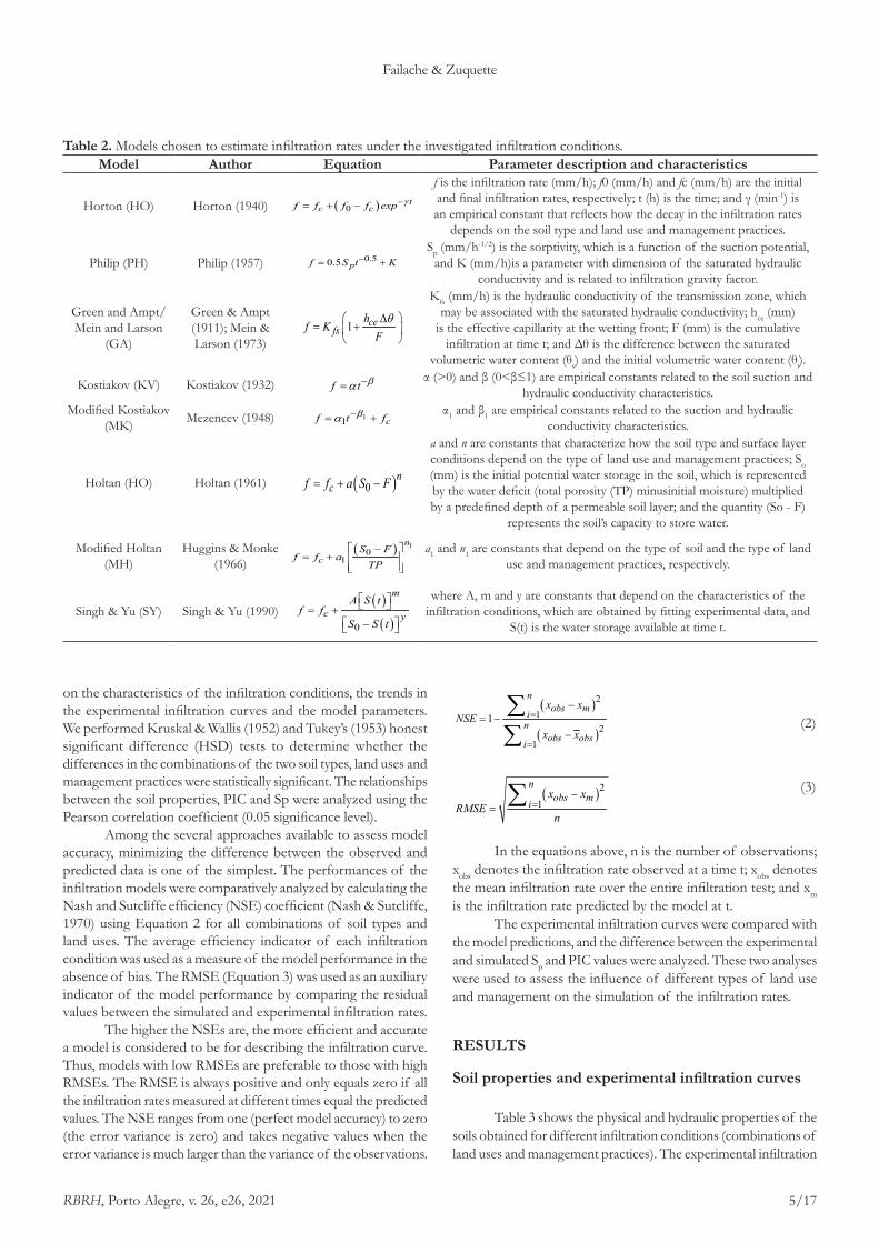
The eight infiltration models used to obtain the simulated infiltration curves, PIC and Sp were chosen based on the ease of obtaining the model input parameters, ease of application and successful application reported in the literature (e.g., Mishra et al., 2003; Sonaje, 2011). The eight selected infiltration models are shown in Table 2.

The parameters of the eight selected infiltration models (f0, fc, γ, Sp, K, Kfs, hce, Δθ, α, β, α1, β1, A, m, y, a, n, So, a1 and n1) were determined using an inverse solution method called the generalized reduced gradient (GRG) method, which is suitable for nonlinear problems, such as the infiltration process (Lasdon et al., 1978; Zakwan et al., 2016). The GRG generates the parameter values that produce the best fit between the infiltration curve obtained in the field and the simulated curve by minimizing the sum of the squared residuals of the infiltration rates. Note that nonempirical models, such as the Philip and Green and Ampt model, were treated as empirical models in this study because the underlying assumptions of the models were typically not satisfied (e.g., the uniformity of the soil properties and the initial water content). Thus, the model parameters were considered unknowns and subjected to a fitting procedure. The independent model parameters, such as F and t, were obtained directly from the infiltration data. However, the S(t) parameter of the Singh and Yu models could not be obtained directly and was determined using Equation 1. This equation involves the initial potential storage (So), the final infiltration rate (fc), the observed initial infiltration rate (fobs(i)) and the observed infiltration rate at time t (fobs(t)) determined in the double-ring tests, where the (t-1) index denotes the preceding interval.

( ) ( ) ( ){ } ( )( )10.5i c obs obs tS t S f f t f i t t − = + − + − (1)

Statistics and evaluation of the results

Basic statistics (e.g., the mean, standard deviation, maximum and minimum) were used to compile and analyze information

RBRH, Porto Alegre, v. 26, e26, 2021

Failache & Zuquette

5/17

on the characteristics of the infiltration conditions, the trends in the experimental infiltration curves and the model parameters. We performed Kruskal & Wallis (1952) and Tukey’s (1953) honest significant difference (HSD) tests to determine whether the differences in the combinations of the two soil types, land uses and management practices were statistically significant. The relationships between the soil properties, PIC and Sp were analyzed using the Pearson correlation coefficient (0.05 significance level).

Among the several approaches available to assess model accuracy, minimizing the difference between the observed and predicted data is one of the simplest. The performances of the infiltration models were comparatively analyzed by calculating the Nash and Sutcliffe efficiency (NSE) coefficient (Nash & Sutcliffe, 1970) using Equation 2 for all combinations of soil types and land uses. The average efficiency indicator of each infiltration condition was used as a measure of the model performance in the absence of bias. The RMSE (Equation 3) was used as an auxiliary indicator of the model performance by comparing the residual values between the simulated and experimental infiltration rates.

The higher the NSEs are, the more efficient and accurate a model is considered to be for describing the infiltration curve. Thus, models with low RMSEs are preferable to those with high RMSEs. The RMSE is always positive and only equals zero if all the infiltration rates measured at different times equal the predicted values. The NSE ranges from one (perfect model accuracy) to zero (the error variance is zero) and takes negative values when the error variance is much larger than the variance of the observations.

( )

( )

21

21

1

nobs mi

nobs obsi

x xNSE

x x

=

=

−= −

−

∑∑

(2)

( )21

nobs mi

x xRMSE

n=

−=∑ (3)

In the equations above, n is the number of observations; xobs denotes the infiltration rate observed at a time t; xobs denotes the mean infiltration rate over the entire infiltration test; and xm is the infiltration rate predicted by the model at t.

The experimental infiltration curves were compared with the model predictions, and the difference between the experimental and simulated Sp and PIC values were analyzed. These two analyses were used to assess the influence of different types of land use and management on the simulation of the infiltration rates.

RESULTS

Soil properties and experimental infiltration curves

Table 3 shows the physical and hydraulic properties of the soils obtained for different infiltration conditions (combinations of land uses and management practices). The experimental infiltration

Table 2. Models chosen to estimate infiltration rates under the investigated infiltration conditions.Model Author Equation Parameter description and characteristics

Horton (HO) Horton (1940) ( )0t

c cf f f f exp γ−= + −

f is the infiltration rate (mm/h); f0 (mm/h) and fc (mm/h) are the initial and final infiltration rates, respectively; t (h) is the time; and γ (min-1) is an empirical constant that reflects how the decay in the infiltration rates

depends on the soil type and land use and management practices.

Philip (PH) Philip (1957) 0.50.5 pf S t K−= +Sp (mm/h-1/2) is the sorptivity, which is a function of the suction potential,

and K (mm/h)is a parameter with dimension of the saturated hydraulic conductivity and is related to infiltration gravity factor.

Green and Ampt/Mein and Larson

(GA)

Green & Ampt (1911); Mein & Larson (1973)

1 ce

fsh

f KFθ∆

= +

Kfs (mm/h) is the hydraulic conductivity of the transmission zone, which may be associated with the saturated hydraulic conductivity; hce (mm)

is the effective capillarity at the wetting front; F (mm) is the cumulative infiltration at time t; and Δθ is the difference between the saturated

volumetric water content (θs) and the initial volumetric water content (θi).

Kostiakov (KV) Kostiakov (1932) f t βa −=α (>0) and β (0<β≤1) are empirical constants related to the soil suction and

hydraulic conductivity characteristics.Modified Kostiakov

(MK) Mezencev (1948) 11 cf t fβa −= +α1 and β1 are empirical constants related to the suction and hydraulic

conductivity characteristics.

Holtan (HO) Holtan (1961) ( )0n

cf f a S F= + −

a and n are constants that characterize how the soil type and surface layer conditions depend on the type of land use and management practices; So (mm) is the initial potential water storage in the soil, which is represented by the water deficit (total porosity (TP) minusinitial moisture) multiplied by a predefined depth of a permeable soil layer; and the quantity (So - F)

represents the soil’s capacity to store water.

Modified Holtan (MH)

Huggins & Monke (1966)

( ) 10

1

n

cS F

f f aTP

−= +

a1 and n1 are constants that depend on the type of soil and the type of land use and management practices, respectively.

Singh & Yu (SY) Singh & Yu (1990)( )

( )0

m

c y

A S tf f

S S t

= + −

where A, m and y are constants that depend on the characteristics of the infiltration conditions, which are obtained by fitting experimental data, and

S(t) is the water storage available at time t.

RBRH, Porto Alegre, v. 26, e26, 20216/17

Soil water infiltration under different land use conditions: in situ tests and modeling

curves and PIC values obtained from in situ tests for the identified land uses and management practice types are shown in Figure 2.

The physical and hydraulic properties of the studied soil vary with the land use type and management practice. The Rhodic Ferralsols are high in clay and silt particles, which are 71.3% of the soil matrix. By contrast, Ferralic Arenosols are sandy soil with 88.3% sand particles. Land use and management practices modify the soil surface layer and therefore, the soil properties. The ρd, n and experimental Sp values of the Rhodic Ferralsols were 1.20 to 1.52 g cm-3, 0.48 to 35.7 mm h-1/2 and 0.59 to 360 mm h-1/2, respectively. Variations in the soil properties of the Ferralic Arenosols were also observed, where the maximum and minimum values of the ρd, n and experimental Sp were 1.42 and 1.58 g cm-3, 0.47 and 764.4 mm h-1/2 and 0.41 and 26.5 mm h-1/2, respectively.

The in situ test results showed a significant variation in the infiltration behavior between the two soil types. The infiltration rates of the Rhodic Ferralsols were generally lower and exhibit less variability than those of the Ferralic Arenosols. The initial section of the infiltration rate curves (up to one minute) exhibited significant variability varying from 1260.0 mm/h (forest-Ferralic Arenosols) to 60 mm/h (sugarcane plantation in the middle of the cycle-Rhodic Ferralsols). The inflection in the infiltration curve for the Rhodic Ferralsols occurred within three minutes for six out of seven land use and management types, compared to between three and seven minutes for the Ferralic Arenosols for four land use and management types and before three minutes

for the remaining types. The average and standard deviation for the PIC for Rhodic Ferralsols were 62.4 mm/h and 73.7 mm/h, respectively, where the lowest and highest values of 8.0 mm/h and 192.0 mm/h, respectively, were obtained for with sugarcane plantations (at the end of the cycle) and banana plantations. The average, standard deviation and maximum and minimum values for the Ferralic Arenosols are 135.3, 202.0, 468.0 and 9.3 mm/h, respectively.

Considering the land use and management practice types independently of the soil types revealed a wide range of behaviors for the infiltration curves presented. The sugarcane, orange plantations and pastures with cattle trampling had lower infiltration rates and PIC and Sp values than pasture without cattle trampling, forests and banana plantations. However, different PIC and Sp values were obtained for the two soils for cultivated forest: 141.0 mm/h and 360.0 mm h-1/2, respectively, for the Rhodic Ferralsols and 18.0 mm/h and 44.0 mm h -1/2, respectively, for the Ferralic Arenosols.

The Ks values measured in the infiltration tests also exhibited variability across the land use and management types, ranging from 6.0 mm/h (Rhodic Ferralsols – sugarcane at the end of the cycle) to 736.8 mm/h (Ferralic Arenosols-forest). The Ks results were generally concordant with the PIC values, except for the Ferralic Arenosols, for which Ks was 268.8 mm/h higher and 199.2 mm/h lower for forest and pasture without cattle trampling, respectively, mainly because of macroporosity.

Table 3. Physical and hydraulic properties of the study soil for different land use types and management practices.

Soil

type

Part

icle

den

sity

(g c

m-3)

Cla

ya (%

)

Silta (

%)

Fine

san

da (%

)

Med

ium

san

d a (

%)

Coa

rse

sand

a (%

)

Text

ureb

Land

use

type

and

soi

l m

anag

emen

t pra

ctic

e

Dry

bul

k de

nsity

(g c

m-3)c

Tota

l por

osity

c

Exp

erim

enta

l sor

ptiv

ity c (

mm

h

-1/2

)

Satu

rate

d hy

drau

lic c

ondu

ctiv

ity

(mm

/h)

Rhodic Ferralsols (Red Latosol in Brazilian soil classification)

2.900 +- 0.067 48.2 +- 11.4 23.1 +- 6.9 21.6 +- 3.9 7.6 +- 1.2 3.1 +- 0.6 Clay Loam Sugarcane plantation (ending of the cycle)

1.520 0.48 37.3 6.8

Sugarcane plantation (middle of the cycle)

1.358 0.54 40.6 13.0

Sugarcane plantation (beginning of the cycle)

1.300 0.57 35.7 40.0

Forest 1.200 0.59 289.0 76.2Cultivated forests 1.425 0.57 360.0 117.5Pasture with cattle

trampling1.500 0.58 54.8.0 79.6

Banana plantation 1.450 0.57 346.8 237.1Ferralic

Arenosols (Quartzarenic

Neosol in Brazilian soil classification)

2.669 +- 0.129 4.3 +- 1.2 7.4 +- 3.2 34.3 +- 3.8 47.4 +- 1.4 6.6 +- 0.3 Sand Sugarcane plantation (ending of the cycle)

1.580 0.41 26.5 12.7

Sugarcane plantation (beginning of the cycle)

1.510 0.43 61.4 86.4

Pasture without cattle trampling

1.440 0.46 718.5 190.8

Forest 1.420 0.47 764.4 736.8Cultivated forests 1.540 0.42 44.0 40.2Pasture with cattle

trampling1.560 0.42 45.1 12.0

Orange plantation 1.570 0.41 41.8 86.4aAverage and standard deviation values obtained for each soil property; bSoil grain size was classified by texture triangle proposed by United States Department of Agriculture (1999); cAverage values obtained for each soil property.

RBRH, Porto Alegre, v. 26, e26, 2021

Failache & Zuquette

7/17

Infiltration model parameters

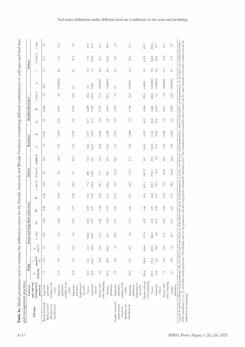
Table 4a and 4b shows the parameters obtained by fitting the experimental infiltration curves to the infiltration model and the initial moisture content determined by the in situ tests.

The parameters representing the gravitational component (K, Kfs, fc and fc1) ranged from 0.1 to 36.7 mm/h for infiltration conditions corresponding to experimental PIC values below 34 mm/h. Thus, the estimated values were in agreement with the values obtained from the in situ tests. There was more significant variation in the parameters for infiltration conditions with higher PIC values. For example, the infiltration capacity observed in the field was 192 mm/h for Rhodic Ferralsols in banana plantations, whereas the estimated parameters ranged from 143 to 219 mm/h. Agreement was also obtained between the parameters that reflect infiltration decay and soil suction (i.e., Sp and Hce) and the experimental Sp parameter, where infiltration conditions with high Sp values resulted in higher values of the respective parameters.

Accuracy and classification of infiltration models

The RMSEs and NSEs reported in Table 5 generally indicate a good fit between the simulated and experimental infiltration curves for nine out of 14 combinations of soil type with land uses and management practices. The models are ranked in order of best to worst accuracy for all infiltration conditions as follows: modified Kostiakov (which most adequately estimated the infiltration rates); Horton; Singh and Yu; modified Holtan; Holtan; Philip; Green and Ampt/Mein and Larson; and Kostiakov, with mean NSEs of 0.964, 0.941, 0.939, 0.936, 0.926, 0.914, 0.912 and

0.905, respectively, and mean RMSEs of 9.87, 11.87, 12.01, 12.55, 13.12, 13.27 13.89 and 17.78 mm/h, respectively.

Simulated infiltration curves

Simulated infiltration curves (Figures 3 and 4) were developed by applying the infiltration parameters to the models (Table 4a and 4b). Figure 5 is a comparison of the Sp and PIC values obtained from the experimental and simulated infiltration curves. The relationship between the PIC and Sp values obtained from the simulated infiltration curves is also shown.

The data presented in Figure 5a show that for the models simulated using infiltration conditions corresponding to experimental PIC values below 34 mm/h, the maximum difference between the estimated and observed values was ±5 mm/h, and the standard deviation between the infiltration models was below 2 mm/h. For infiltration conditions corresponding to experimental PIC values between 35 and 200 mm/h, the maximum difference between the observed and predicted values was ±29 mm/h, with a standard deviation between the infiltration models of approximately 9 mm/h. However, the data with the highest dispersion were obtained under infiltration conditions corresponding to experimental PIC values above 300 mm/h, where the maximum difference between the observed and predicted values was ±38 mm/h and the standard deviation between the infiltration models was higher than 15 mm/h. Figure 5b shows a good fit was obtained for the combination of soil type with land use and management practices corresponding to experimental Sp values below 30 mm h-1/2, where the differences between the measured and predicted values were below ±1.8 mm h-1/2. However, differences up to ±20 mm h-1/2 and

Figure 2. Experimental infiltration curves for study soils (Ferralic Arenosols and Rhodic Ferralsols) with different land uses and management practices.

RBRH, Porto Alegre, v. 26, e26, 20218/17

Soil water infiltration under different land use conditions: in situ tests and modelingTa

ble

4a. M

odel

par

amet

ers u

sed

to e

stim

ate

the

infil

tratio

n cu

rves

for t

he F

erra

lic A

reno

sols

and

Rhod

ic F

erra

lsols

cons

ider

ing

diff

eren

t com

bina

tions

of

soil

type

s and

land

use

s an

d m

anag

emen

t pra

ctic

es.

Soil

type

Land

use

ty

pe a

nd s

oil

man

agem

ent

prac

tices

Phili

pG

reen

and

am

pt-M

ein

and

Lars

onH

orto

nK

ostia

kov

Mod

ified

Kos

tiako

vH

olta

n

K (m

m/h

)

S p (m

m/h

-

1/2 )

K fs (m

m/h)

h ce (mm

)∆θ

θsaθ ib

fc (m

m/h)

fi (m

m/h)

γ (m

in-1)

αβ

α 1β 1

f c (mm

/h)

an

fc (m

m/h)

s o (mm

)

Rhod

ic F

erra

lsols

(Red

Lat

osol

in

Braz

ilian

soil

clas

sifica

tion)

Suga

rcan

e pl

anta

tion

(end

ing

of th

e cy

cle)

1.5

13.0

6.7

32.0

0.20

0.48

0.28

10.8

9533

.57.

20.

487

3.9

0.60

85.

020

.01.

211

.12.

9

Suga

rcan

e pl

anta

tion

(mid

dle

of th

e cy

cle)

11.5

9.5

17.0

6.2

0.24

0.54

0.30

17.3

6418

.815

.00.

289

10.5

0.34

94.

90.

0000

016.

617

.215

.2

Suga

rcan

e pl

anta

tion

(beg

inni

ng o

f th

e cy

cle)

12.8

9.2

16.6

5.6

0.32

0.57

0.25

20.3

9755

.215

.50.

278

0.6

0.93

518

.60.

34.

120

.34.

0

Fore

st25

.081

.115

.781

2.6

0.34

0.59

0.25

77.8

880

33.2

46.3

0.57

125

.70.

689

36.6

2.0

1.8

77.5

31.9

Cul

tivat

ed

fore

sts

49.8

164.

592

.833

0.0

0.27

0.57

0.30

162.

811

5830

.111

6.3

0.43

414

.30.

932

136.

80.

001

3.3

162.

267

.9

Past

ure

with

ca

ttle

tram

plin

g6.

925

.814

.353

.30.

260.

580.

3224

.717

229

.318

.20.

430

4.4

0.76

317

.20.

0000

076.

225

.116

.3

Bana

na

plan

tatio

n14

3.2

89.4

184.

264

.70.

240.

570.

3321

9.4

938

54.5

170.

20.

258

6.8

0.90

119

9.1

0.00

0003

4.0

243.

699

.9

Ferr

alic

Are

noso

ls (Q

uart

zare

nic

Neo

sol i

n Br

azili

an so

il cl

assifi

catio

n)

Suga

rcan

e pl

anta

tion

(end

ing

of th

e cy

cle)

1.9

10.5

4.3

28.6

0.27

0.41

0.14

11.0

113.

668

.35.

10.

524

0.5

1.02

59.

20.

35.

010

.63.

4

Suga

rcan

e pl

anta

tion

(beg

inni

ng o

f th

e cy

cle)

30.0

13.1

36.7

5.4

0.33

0.43

0.11

41.0

133.

647

.234

.20.

208

2.2

0.72

836

.00.

0000

16.

540

.911

.3

Past

ure

with

out

cattl

e tra

mpl

ing

306.

816

0.8

404.

667

.80.

290.

460.

1441

1.3

1367

.926

.735

4.5

0.23

558

.20.

566

335.

20.

0004

3.0

412.

911

9.7

Fore

st29

9.5

375.

342

3.1

288.

40.

380.

470.

0855

2.5

2730

.129

.545

2.2

0.32

138

.40.

886

485.

60.

0000

013.

855

0.0

255.

4C

ultiv

ated

fo

rest

s18

.48.

124

.22.

80.

270.

420.

1320

.352

.46.

021

.00.

214

21.0

0.21

40.

10.

0000

034.

620

.033

.7

Past

ure

with

ca

ttle

tram

plin

g7.

115

.013

.417

.90.

290.

420.

1217

.210

1.8

26.3

12.9

0.39

85.

40.

567

9.8

0.00

0003

6.3

16.2

15.5

Ora

nge

plan

tatio

n4.

715

.69.

329

.70.

270.

410.

1218

.014

6.4

56.5

10.0

0.46

40.

90.

950

14.9

0.00

0001

8.7

17.5

9.1

Lege

nd: K

and

Sp

are

Phili

p m

odel

par

amet

ers;

Kfs,

Hce,

∆θ,

θs a

nd θ

i are

Gre

en a

d A

mpt

-Mei

n an

d La

rson

mod

el p

aram

eter

s; fc,

fi a

nd γ

are

Hor

ton’s

mod

el p

aram

eter

s; α

and

β ar

e K

ostia

kov

mod

el p

aram

eter

s; α1

, β1,

and

fc1 a

re m

odifi

ed K

ostia

kov

mod

el p

aram

eter

s; a,

n, f c,

S o are

Hol

tan

mod

el p

aram

eter

s. a T

he a

dopt

ed v

alue

of

this

para

met

er w

as th

e to

tal p

oros

ity o

btai

ned

by la

bora

tory

test

s b The

con

sider

ed in

itial

vol

umet

ric w

ater

con

tent

was

the

valu

e ob

tain

ed in

the

field

con

ditio

n be

fore

the

infil

tratio

n te

st b

egin

ning

.

RBRH, Porto Alegre, v. 26, e26, 2021

Failache & Zuquette

9/17

a trend toward smaller simulated values were observed for infiltration conditions corresponding to experimental Sp values above 200 mm h-1/2. Differences of up to ±11.2 mm h-1/2 were observed for infiltration conditions corresponding to experimental Sp values between 100 and 200 mm h-1/2.

DISCUSSION

General comments

The main study results show different soil properties and infiltration rates for Ferralic Arenosols and Rhodic Ferralsols, as well as for different land uses and management practices. The infiltration capacity and Sp was not clearly correlated with studied soil properties (n, ρd, ρs and texture) for more than 40% of the infiltration conditions. Different model fits were obtained under different infiltration conditions. The models are ranked in order of best to worst accuracy as follows: modified Kostiakov (the model that most adequately estimated the infiltration rates), Horton; Singh and Yu; modified Holtan; Holtan; Philip; Green and Ampt/Mein and Larson and Kostiakov.

The procedures used in the study enabled us to determine and characterize the basic properties and infiltration behavior of soil and to evaluate the ability of infiltration models to simulate infiltration curves under different infiltration conditions. Although good results are obtained using the double ring method (Bouwer, 1969), which can be used to determine infiltration rates of large areas, a considerable quantity of water and time are needed to characterize

several infiltration conditions. Thus, faster methods that use lower water volumes are essential for infiltration studies on large areas to obtain an overview of the infiltration behavior of a study region. Indicators of the model performance were used for two soil types with different land use and management in this study and permitted to evaluate those infiltration conditions. Having briefly reviewed the main results and analyzed the study methodology, we assess the results and discuss the potential implications.

Soil characteristics and infiltration behavior

Different soil characteristics and infiltration behavior were obtained under different infiltration conditions in this study. A linear regression (Figure 6d and 6e) showed the PIC of the Ferralic Arenosols was strongly negatively and positively correlated with ρd and n, respectively, with R2 values of 0.90 and 0.94, respectively. This result is a statistical indication that the infiltration capacity is strongly affected by land use and management. However, the absence of a clear correlation between the PIC and soil properties for the Rhodic Ferralsols (Figure 6a and 6b) was attributed to macroporosity, as observed by Fagundes & Zuquette (2012) and Failache (2018), which can significantly modify infiltration rates in these soil types. Thus, the properties of the two studied soils do not adequately explain the infiltration behavior for the Rhodic Ferralsols, because the PIC could not be clearly correlated with the soil properties under all the infiltration conditions studied.

As previously discussed, the linear regression analysis did not show a statistically significant correlation between the PIC and the

Table 4b. (cont.) Model parameters used to estimate the infiltration curves for the Ferralic Arenosols and Rhodic Ferralsols considering different combinations of soil types and land uses and management practices

Soil typeLand use type and soil management

practices

Modified Holtana Singh and Yu

a1 n1

fc (mm/h) so (mm) A m y fc (mm/h) s

o (mm)

Rhodic Ferralsols (Red Latosol in Brazilian soil classification)

Sugarcane plantation (ending

of the cycle)9.0 1.2 11.1 2.9 3,00E-02 0 10.11 10.8 53.9

Sugarcane plantation (middle

of the cycle)0.00001 5.3 17.3 12.3 2.34 0.709 0.36 0 40.9

Sugarcane plantation

(beginning of the cycle)

0.2 3.2 20.4 3.2 0.85 0 3.29 19.1 65.0

Forest 0.00002 3.8 75.1 51.4 0.81 1.678 1.43 62.4 135.3Cultivated forests 0.000002 3.9 161.7 76.0 1.29 1.575 0 152.6 31.1Pasture with cattle

trampling 0.000001 5.4 25.2 14.7 0.86 1.149 0.29 0 42.0

Banana plantation 0.1 2.0 221.7 27.2 1279.91 0 1.57 203.3 58.0

Ferralic Arenosols (Quartzarenic

Neosol in Brazilian soil classification)

Sugarcane plantation (ending

of the cycle)0.02 4.5 10.7 3.0 9,00E-07 0.003 22.69 12.8 5.1

Sugarcane plantation

(beginning of the cycle)

0.000006 6.8 42.9 5.6 3.60 0.807 0.21 20.5 19.2

Pasture without cattle trampling 0.00004 3.0 413.0 119.7 1.63 1.955 1.47 403.0 62.3

Forest 0.000002 3.3 534.5 232.8 388.43 0.066 0.00 554.4 14.5Cultivated forests 0.02 2.1 21.2 15.1 2.30 0.959 0.25 2.4 18.4Pasture with cattle

trampling 0.000003 5.3 16.9 11.6 1.42 0.782 1.13 12.9 35.6

Orange plantation 0.000001 6.7 17.7 7.2 1.37 0.808 0.65 9.2 37.8Legend: a, n, fc, So are Holtan model parameters.; a, m, n, fc and So are Singh and Yu model parameters. athe total porosity for each infiltration condition is presented in Table 1.

RBRH, Porto Alegre, v. 26, e26, 202110/17

Soil water infiltration under different land use conditions: in situ tests and modeling

Table 5. Statistical parameters for the results obtained by infiltration modeling.

Soil type

Land use and

management practice

Model RMSE (mm/h) NSE

Model classification

based on NSE values

*1

Soil type

Land use and

management practice

Model RMSE (mm/h) NSE

Model classification

based on NSE values

*1

Rhodic Ferralsols

Sugarcane plantation (ending of the cycle)

PH 3.20 0.922 G Ferralic Arenosols

Sugarcane plantation (ending of the cycle)

PH 3.50 0.896 STGA 3.65 0.871 ST GA 3.59 0.900 GHO 3.16 0.960 VG HO 1.88 0.970 VGKV 3.66 0.919 G KV 4.03 0.889 STKM 2.86 0.927 G KM 1.47 0.981 VGHT 3.62 0.945 G HT 2.00 0.967 VGHM 3.62 0.945 G HM 2.07 0.966 VGSY 3.29 0.932 G SY 3.79 0.849 ST

Sugarcane plantation (middle of the cycle)

PH 4.56 0.846 ST Sugarcane plantation (middle of the cycle)

PH 3.18 0.920 G GA 4.56 0.846 ST GA 3.87 0.918 G HO 3.33 0.893 ST HO 6.04 0.826 STKV 2.27 0.937 G KV 4.31 0.854 STKM 2.21 0.939 G KM 3.53 0.933 GHT 3.24 0.893 ST HT 6.16 0.820 STHM 3.27 0.891 ST HM 6.74 0.813 STSY 3.63 0.860 ST SY 1.77 0.984 VG

Sugarcane plantation

beginning of the cycle)

PH 3.23 0.906 G Pasture without cattle

trampling

PH 42.89 0.921 GGA 2.57 0.941 G GA 57.56 0.878 STHO 1.85 0.961 VG HO 32.64 0.960 VGKV 4.90 0.805 ST KV 63.70 0.836 STKM 1.73 0.971 VG KM 44.24 0.929 GHT 1.95 0.958 VG HT 30.00 0.963 VGHM 1.99 0.955 VG HM 30.00 0.963 VGSY 1.47 0.978 VG SY 36.19 0.942 G

Forest PH 35.32 0.822 ST Forest PH 33.35 0.956 VGGA 18.91 0.975 VG GA 33.18 0.951 VGHO 17.72 0.984 VG HO 37.03 0.955 VGKV 20.68 0.978 VG KV 55.50 0.907 GKM 13.07 0.985 VG KM 31.83 0.959 VGHT 17.93 0.985 VG HT 37.90 0.954 VGHM 17.11 0.986 VG HM 38.91 0.951 VGSY 24.51 0.955 VG SY 45.88 0.912 G

Cultivated forests

PH 28.12 0.933 G Cultivated forests

PH 2.93 0.897 STGA 22.71 0.960 VG GA 5.29 0.708 UTHO 17.23 0.982 VG HO 1.66 0.968 VGKV 37.89 0.910 G KV 1.25 0.980 VG KM 13.12 0.986 VG KM 1.26 0.980 VG HT 17.64 0.981 VG HT 1.40 0.975 VGHM 17.38 0.981 VG HM 2.03 0.957 VGSY 27.10 0.925 G SY 1.95 0.945 G

Pasture with cattle trampling

PH 4.57 0.947 G Pasture with cattle trampling

PH 1.27 0.990 VGGA 4.22 0.961 VG GA 2.31 0.975 VGHO 6.10 0.917 G HO 2.43 0.979 VGKV 5.22 0.934 G KV 2.27 0.977 VGKM 3.85 0.967 VG KM 1.15 0.992 VGHT 5.83 0.923 G HT 2.09 0.983 VGHM 5.89 0.922 G HM 2.10 0.985 VGSY 4.61 0.946 G SY 2.14 0.968 VG

Banana plantation

PH 24.36 0.931 G Orange plantation

PH 3.91 0.913 G GA 17.88 0.960 VG GA 3.41 0.922 G HO 29.38 0.918 G HO 5.17 0.896 STKV 37.96 0.843 ST KV 5.32 0.894 STKM 15.44 0.977 VG KM 2.47 0.967 VGHT 51.31 0.710 UT HT 4.73 0.902 GHM 32.08 0.893 ST HM 4.90 0.898 STSY 17.03 0.970 VG SY 2.34 0.977 VG

Legend: PH = Philip’s model; GA = Green and Ampt-Mein and Larson model; HO = Horton’s model ; KV = Kostiakov’s model; KM = Modified Kostiakov’s model; HT = Holtan model; HM = Modified Holtan model; SY = Sing and Yu model; ST = Satisfactory; UT = Unsatisfactory; G = Good; VG = Very Good; 1*Classification based on Mishra et al. (2003) proposition.

RBRH, Porto Alegre, v. 26, e26, 2021

Failache & Zuquette

11/17

analyzed soil properties for one of the studied soils. However, lower infiltration rates and PIC values were found for the combinations of soil type and land uses that generally correspond to highly compacted conditions and vice versa. For example, the land uses and management practices (e.g., sugarcane, orange plantation, pasture with cattle trampling) that produced the highest dry ρd values for

Ferralic Arenosols (> 15 kN/m3) corresponded to much lower PIC values (34 mm/h) than combinations with lower ρd values (PIC > 390 mm/h). For the Rhodic Ferralsols, the two infiltration conditions corresponding to high compaction (pasture with cattle trampling and sugarcane at the end of the cycle) also corresponded to the two lowest PIC values; however, cultivated forest and banana

Figure 3. Comparison of the experimental and modeled infiltration rates for Rhodic Ferralsols. Legend: PH (Philip), GA (Green and Ampt-Mein and Larson), HO (Horton), KV (Kostiakov), KM (modified Kostiakov), HT (Holtan), HM (modified Holtan) and SY (Singh and YU).

RBRH, Porto Alegre, v. 26, e26, 202112/17

Soil water infiltration under different land use conditions: in situ tests and modeling

plantation had a high ρd (> 1.4 g cm-3), as previously mentioned, and macroporosity affected the infiltration behavior.

Performing a linear regression on PIC and Ks (Figure 7c and 7f) produced a positive correlation with an R2 of 0.86 and 0.72 for

Rhodic Ferralsols and Ferralic Arenosols, respectively, indicating that reliable PIC values were measured in the infiltration tests. The main variability found in the Ferralic Arenosols (forest and pasture without cattle trampling) may be attributed to the test area,

Figure 4. Comparison of the experimental and modeled infiltration rates for Ferralic Arenosols. Legend: PH (Philip), GA (Green and Ampt-Mein and Larson), HO (Horton), KV (Kostiakov), KM (modified Kostiakov), HT (Holtan), HM (modified Holtan) and SY (Singh and YU).

RBRH, Porto Alegre, v. 26, e26, 2021

Failache & Zuquette

13/17

which is considered large for double-ring infiltrometer tests, and can exhibit a high macroporosity.

The infiltration curves in Figure 3 show three distinct regimes for the infiltration rate: between the beginning of the test and the beginning of the inflection point, the inflection region and the end of the curve. Significant variability in the infiltration rates was observed over the first regime. Infiltration rates below 120 mm/h were observed for land use types producing intense compaction and particle rearrangement of the soil (sugarcane and orange plantations and pasture with cattle trampling). However, high infiltration rates ranging from 700 mm/h to approximately 1200 mm/h were observed for the land use types that do not produce such intense compaction and are attributed to the strong influence of the macroporosity on infiltration and the water deficit

(θs - θi), i.e., the higher the water deficit was, the higher the infiltration rate was. To determine the size and extension of the macropores and better explain the infiltration rates, cross sections were taken of the samples used in the saturated hydraulic conductivity tests. The macropore size varied from 0.1 mm to more than 8 mm for the Rhodic Ferralsols (banana plantation) and Ferralic Arenosols (forest) (see Figure 7a and 7b, respectively). This macroporosity was primarily induced by roots and animals. In most samples in which microporosity was identified, the pores were completely or partially connected.

The inflection in the infiltration curve generally occurred before three minutes of testing under high compaction conditions. However, the inflection occurred between three and seven minutes for the other land use and management types, which may be attributed

Figure 5. Comparison between experimental and simulated data: (a) potential infiltration capacity and (b) sorptivity. Legend: PH (Philip), GA (Green and Ampt-Mein and Larson), HO (Horton), KV (Kostiakov), KM (modified Kostiakov), HT (Holtan), HM (modified Holtan) and SY (Singh and YU).).

Figure 6 Linear regression of experimental potential infiltration capacity with soil properties (dry bulk density, total porosity and saturated hydraulic conductivity): (a), (b) and (c) correspond to the Rhodic Ferralsols; (d), (e) and (f) correspond to the Ferralic Arenosols.

RBRH, Porto Alegre, v. 26, e26, 202114/17

Soil water infiltration under different land use conditions: in situ tests and modeling

to the high porosity and presence of macropores in these soils, which increase the time required to fill pores with water. The final portion of the curve for infiltration conditions corresponding to PIC values below 100 mm/h tended to stabilize faster before the PIC was reached. Infiltration conditions corresponding to PIC values above 100 mm/h produced a higher variation in the infiltration rates and a longer time for stabilization. This result can be attributed to the longer time required for water to fill the macropores identified in the soils with the respective land uses and management.

The Kruskal-Wallis and Tukey tests were used to determine whether there were significant differences between the combinations of soil types and land use and management considering the PIC values. The p value from the Kruskal-Wallis test was lower than the 0.05 significance level, indicating that the median of the population of the groups was not equal; thus, there were differences between the infiltration conditions. Two main groups of infiltration conditions were identified based on the Tukey test. The first group corresponded to the Ferralic Arenosols, with sugarcane at the beginning and end of the cycle, orange plantations, pasture with cattle trampling and cultivated forest and the Rhodic Ferralsols with sugarcane at the beginning, middle and end of the cycle and pasture with cattle trampling. A maximum average PIC of 34 mm/h was reached under these infiltration conditions. The second group corresponded to the Rhodic Ferralsols with cultivated forest, forest and banana plantations and the Ferralic Arenosols with pasture without cattle trampling and forests, which corresponded to average PIC values above 48 mm/h. However, the infiltration conditions within the second group were not equivalent, that is, these conditions did not correspond to the same statistical behavior. These results corroborate the soil characterization and infiltration data showing that land use and management affect infiltration behavior and rates.

Infiltration model evaluation

Good results were generally obtained using the considered infiltration models for most infiltration conditions. A comprehensive

and qualitative analysis of the mean statistical indicators for all the infiltration conditions was used to evaluate the selected models more generally in terms of accuracy and the infiltration curves generated for the different infiltration conditions. Mishra et al.’s (2003) proposition was used as the evaluation criterion: infiltration conditions with NSEs between 1 and 0.95, 0.95 and 0.90, 0.90 and 0.75 and less than 0.75 were classified as very good, good, satisfactory and unsatisfactory, respectively.

Considering the NSEs for all the infiltration conditions, only the modified Kostiakov model fell into the very good class, whereas the other models were classified as good. The modified Kostiakov model outperformed the other models in terms of lower RMSEs. Zolfaghari et al. (2012) and Sihag et al. (2017) similarly found that the modified Kostiakov model fit measured data better than other models. Bayabil et al. (2019) and Mishra et al. (2003) found that the Horton and Singh and Yu models provided good fits to infiltration data, which is consistent with the results obtained in this study that these two models produced the second and third most accurate simulated infiltration rates. The Kostiakov and Green and Ampt and Philip models exhibited the worst performance and generated the highest residual values among the considered models. Jačka et al. (2016) reported similarly high RMSEs using the Philip and Green and Ampt/Mein and Larson models.

Separate analyses of the land uses and management practices showed that for the nine infiltration conditions corresponding to high compaction, few macropores and infiltration capacities below 35 mm/h, accurate simulated infiltration curves were obtained with RMSEs below 5 mm/h and a low standard deviation for the estimated PIC and Sp. However, for the five infiltration conditions corresponding to low compaction, high macroporosity and measured PIC values above 35 mm/h, a high RMSE was obtained, as well a large dispersion in the simulated PIC and Sp values relative to the experimental values. These infiltration conditions correspond to banana plantations, cultivated forest and forest with Rhodic Ferralsols and forest and pasture without cattle trampling with Ferralic Arenosols, which produced RMSEs

Figure 7. Cross section of samples used in saturated hydraulic conductivity test showing the presence of macropores in (a) Rhodic Ferralsols (banana plantation) and (b) Ferralic Anenosols (forest).

RBRH, Porto Alegre, v. 26, e26, 2021

Failache & Zuquette

15/17

above 15 mm/h in practically all the analyzed models. Note that applying the modified Kostiakov model to pasture without cattle trampling and with Ferralic Arenosols produced RSMEs of up to 63.0 mm/h. Suryoputro et al. (2018) obtained a similarly high RMSE by applying models to forest, which was considered unsatisfactory performance.

These high RMSEs are attributed to the infiltration data obtained in the field in this study. These data include the effect of soil heterogeneity and macroporosity (as previously identified by Fagundes & Zuquette (2012), Failache (2018) and in this study) under the considered infiltration conditions, which resulted in erratic infiltration rates. The considered models were not designed to be applied under conditions of heterogeneity and macroporosity, i.e., the characteristics of the infiltration conditions (hydraulic conductivity, initial moisture, porosity and suction) did not meet the assumptions and boundary conditions of the models. Thus, the simulated infiltration curves did not fit the data well, resulting in poor model performance.

A comparison of the types of model used to simulate the infiltration conditions in the presence of macroporosity and heterogeneity generally showed physical models performed below empirical models. However, the physical models tended to be more accurate for analyzing land uses and management practices that produce high compaction and homogenization of the soil structure. For example, applying the Green and Ampt/Mein and Larson model to pasture with cattle trampling and Rhodic Ferralsols produced the second-best performance for this infiltration condition. This result is corroborated by that of Mishra et al. (2003), who found a high accuracy using physical models to simulate infiltration rates based on laboratory data, which are more homogeneous than those based on field data and therefore agree well with experimental results.

Other models with more parameters could be applied to infiltration conditions that do not conform to the assumptions made in the commonly used infiltration models considered in this study. Although increasing the number of parameters generally improves model performance, overparameterization may occur, and parameter uncertainty may increase (Perrin et al., 2001). To solve this problem, an optimum model with the lowest number of fitting parameters for the same fitting condition could be defined using several statistical techniques, such as the F-statistic (Green & Caroll 1978), the F-statistic and Cp statistic of Mallows (1973) and the Akaike information criterion (AIC) (Carrera & Neuman 1986). It is important to consider that the best model for a specific infiltration condition may not be applicable to all types of problems.

CONCLUSIONS

High variability is observed for data obtained for different combinations of soils with land uses and management practices. Thus, different conditions for a hydrographic basin, in terms of infiltration and runoff rates, can be generated depending on the predominant combination in the basin that can change from one year to the next. The specific land uses and management practices developed in a basin can be used as basic input to a selected

model to simulate infiltration behavior and forecast potential environmental problems, such as erosion and flooding.

The estimated parameters reflecting the gravitational and matrix components in the infiltration models were significantly influenced by the macroporosity, void ratio and porosity. These parameters were considerably higher for infiltration conditions corresponding to high macroporosity, void ratios and porosities than for more compacted and homogeneous infiltration conditions.

The modified Kostiakov, Horton and Singh and Yu models can be applied to accurately estimate infiltration rates for the land use and management types used with Ferralic Arenosols and Rhodic Ferralsols. The Kostiakov model exhibited the worst performance among the investigated models by underestimating or overestimating the infiltration rates. The modified Holtan, Holtan, Philip and Green and Ampt/Mein and Larson models exhibited satisfactory to good performance in estimating the infiltration rates under eight infiltration conditions. The land uses and management practices affected the accuracy of the selected infiltration models. Poor model performance was generally observed for land uses and management practices that produced low-compaction soil layers with high porosities and void ratios, high degree of macroporosity and heterogeneity, which generated an erratic infiltration behavior. By contrast, the most accurately simulated infiltration rates were obtained for conditions corresponding to land uses and management practices that produced high compaction and low porosities and void ratios.

ACKNOWLEDGEMENTS

Financial support for this study was provided by the São Paulo Research Foundation (FAPESP) [No. 2014/02162-0].

REFERENCES

Almeida, W. S., Panachuki, E., Oliveira, P., Menezes, R., Sobrinho, T., & Carvalho, D. (2018). Effect of soil tillage and vegetal cover on soil water infiltration. Soil & Tillage Research, 175, 130-138. http://dx.doi.org/10.1016/j.still.2017.07.009.

American Society for Testing and Materials – ASTM. (2018). ASTM D3385-18: standard test method for infiltration rate of soils in field using double-ring infiltrometer. West Conshohocken: ASTM International.

Associação Brasileira de Normas Técnicas – ABNT. (1984). NBR 6508: solo, determinação da massa específica aparente (8 p.). Rio de Janeiro: ABNT.

Associação Brasileira de Normas Técnicas – ABNT. (1995). NBR 6502: rochas e solos: análise granulométrica conjunta (18 p.). Rio de Janeiro: ABNT.

Bayabil, B., Dile, Y., Tebebu, T., Engda, T., & Steenhuis, T. (2019). Evaluating infiltration models and pedotransfer functions: implications for hydrologic modeling. Geoderma, 338, 159-169. http://dx.doi.org/10.1016/j.geoderma.2018.11.028.

RBRH, Porto Alegre, v. 26, e26, 202116/17

Soil water infiltration under different land use conditions: in situ tests and modeling

Bouwer, H., (1969). Infiltration of water into nonuniform soil. Journal of Irrigation and Drainage Engineering, 95, 451-462.

Bouwer, H. (1986). Intake rate: cylinder infiltrometer. In A. Klute (Ed.), Methods of soil analysis, part 1: physical and mineralogical methods (pp. 825-844). Wisconsin: SSSA.

Carrera, J., & Neuman, S. P. (1986). Estimation of aquifer parameters under transient and steady state conditions: 1. Maximum likelihood incorporating prior information. Water Resources Research, 22(2), 199-210. http://dx.doi.org/10.1029/WR022i002p00199.

Darcy, H. (1856). Exposition et application des principes a suivre et des formulesa employer dans les questions de distribution d’eau. In V. Dalmont (Ed.), Les Fontaines Publiques de la Ville de Dijon. Paris: Dalmont.

Empresa Brasileira de Pesquisa Agropecuária – EMBRAPA. (1981). Levantamento pedológico semi-detalhado do Estado de São Paulo, 1:100.000 scale. Brasília: EMBRAPA.

Empresa Brasileira de Pesquisa Agropecuária – EMBRAPA. (2018). Sistema Brasileiro de Classificação de Solos (5. ed.). Brasília: EMBRAPA.

Fagundes, J. R. T., & Zuquette, L. V. (2012). Avaliação das características de infiltração de materiais inconsolidados residuais da Formação Botucatu considerando macroporosidades. In Anais do VI Congresso Luso-Brasileiro de Geotecnia, Lisboa.

Failache, M. (2018). Proposta de procedimentos para a estimativa de infiltração potencial e do escoamento superficial Hortoniano potencial baseada em dados geológicos, geotécnicos, de uso e ocupação e eventos de chuva (PhD thesis). Geotechnics Department, University of São Paulo, São Carlos.

Failache, M., & Zuquette, L. (2018). Geological and geotechnical land zoning for potential Hortonian overland flow in a basin in southern Brazil. Engineering Geology, 246, 107-122. http://dx.doi.org/10.1016/j.enggeo.2018.09.032.

Food and Agriculture Organization – FAO. (2015). World reference base for soil resources 2014 International soil classification system for naming soils and creating legends for soil map. Rome: FAO.

Gifford, G. F. (1976). Applicability of some infiltration formula to rangeland infiltrometer data. Journal of Hydrology, 28(1), 1-11. http://dx.doi.org/10.1016/0022-1694(76)90048-2.

Green, P. E., & Caroll, J. D. (1978). Analyzing multivariate data. New York: John Wiley & Sons.

Green, W. H., & Ampt, G. (1911). Studies on soil physics, 1. The flow of air and water through soils. Journal of Agricultural Science, 4, 1-24. http://dx.doi.org/10.1017/S0021859600001441.

Holtan, H. N. (1961). A concept for infiltration estimates in watershed engineering (Bulletin, No. 41-51). Washington: Agricultural Research Service, U.S. Department of Agriculture

Horton, R. E. (1940). An approach toward a physical interpretation of infiltration-capacity. Soil Science Society of America Journal, 5(C), 399-417. http://dx.doi.org/10.2136/sssaj1941.036159950005000C0075x.

Huggins, L. F., & Monke, E. J. (1966). The mathematical simulation of the hydrology of small watersheds (Technical Report, No. 1, 130 p.). Indiana: Resources Research Center, Purdue University Water.

Jačka, L., Pavlásek, J., Pech, P., & Kuráž, V. (2016). Assessment of evaluation methods using infiltration data measured in heterogeneous mountain soils. Geoderma, 276, 74-83. http://dx.doi.org/10.1016/j.geoderma.2016.04.023.

Klute, A., & Dirksen, C. (1986). Hydraulic conductivity and diffusivity: laboratory methods. In A. Klute (Ed.), Methods of soil analysis, part 1 (2nd ed., pp. 687-734, Agronomy Monograph, No. 9). Madison: American Society of Agronomy.

Kostiakov, A. N. (1932). On the dynamics of the coefficient of water-percolation in soils and on the necessity for studying it from a dynamic point of view for purposes of amelioration. Soviet Soil Science, 14, 17-21.

Kruskal, W. H., & Wallis, W. A. (1952). Use of ranks in one-criterion variance analysis. Journal of the American Statistical Association, 47(260), 583-621. http://dx.doi.org/10.1080/01621459.1952.10483441.

Lasdon, L. S., Waren, A. D., Jain, A., & Ratner, M. (1978). Design and testing of a generalized reduced gradient code for nolinear programming. ACM Transactions on Mathematical Software, 4(1), 34-50. http://dx.doi.org/10.1145/355769.355773.

Machiwal, D., Jha, M. K., & Mal, B. C. (2006). Modelling infiltration and quantifying spatial soil variability in a watershed of Kharagpur, India. Biosystems Engineering, 95(4), 569-582. http://dx.doi.org/10.1016/j.biosystemseng.2006.08.007.

Mallows, C. L. (1973). Some comments on Cp. Technometrics, 15(4), 661-675. http://dx.doi.org/10.2307/1267380.

Mein, R., & Larson, C. (1973). Modelling infiltration during a steady rain. Water Resources Research, 9(2), 384-394. http://dx.doi.org/10.1029/WR009i002p00384.

Mezencev, V. J. (1948). Theory of formation of the surface runoff. Meteorologia i Gidrologia, 3, 33-40.

Mirzaee, S., Zolfaghari, A. A., Gorji, M., Dyck, M., & Ghorbani Dashtaki, S. (2014). Evaluation of infiltration models with different numbers of fitting parameters in different soil texture classes. Archives of Agronomy and Soil Science, 60(5), 681-693. http://dx.doi.org/10.1080/03650340.2013.823477.

Mishra, S. K., Tyagi, J. V., & Singh, V. P. (2003). Comparison of infiltration models. Hydrological Processes, 17(13), 2629-2652. http://dx.doi.org/10.1002/hyp.1257.

RBRH, Porto Alegre, v. 26, e26, 2021

Failache & Zuquette

17/17

Nash, J. E., & Sutcliffe, J. V. (1970). River flow forecasting through conceptual models part I: a discussion of principles. Journal of Hydrology, 10(3), 282-290. http://dx.doi.org/10.1016/0022-1694(70)90255-6.

Oliveira, J. C., Vaz, C. M., & Reichardt, K. (1995). Efeito do cultivo contínuo da cana-de-açúcar em propriedades físicas de um Latossolo Vermelho Escuro. Scientia Agrícola, 52(1), 50-55. http://dx.doi.org/10.1590/S0103-90161995000100009.

Peel, M. C., Finlayson, B. L., & Mcmahon, T. A. (2007). Updated world map of the Köppen-Geiger climate classification. Hydrology and Earth System Sciences, 11(5), 1633-1644. http://dx.doi.org/10.5194/hess-11-1633-2007.

Perrin, C., Michel, C., & Andréassian, V. (2001). Does a large number of parameters enhance model performance? comparative assessment of common catchment model structures on 429 catchments. Journal of Hydrology, 242(3-4), 275-301. http://dx.doi.org/10.1016/S0022-1694(00)00393-0.

Philip, J. R. (1957). The theory of infiltration: 1. The infiltration equation and its solution. Soil Science, 83(5), 345-358. http://dx.doi.org/10.1097/00010694-195705000-00002.

Shao, Q., & Baumgartl, T. (2014). Estimating input parameters for four infiltration models from basic soil, vegetation, and rainfall properties. Soil Science Society of America Journal, 78(5), 1507-1521. http://dx.doi.org/10.2136/sssaj2014.04.0122.

Shukla, M. K., Lal, R., Owens, L. B., & Unkefer, P. (2003). Land use and management impacts on structure and infiltration characteristics of soils in the North Appalachian region of Ohio. Soil Science, 168(3), 167-177. http://dx.doi.org/10.1097/01.ss.0000058889.60072.aa.

Sihag, P., Tiwari, N., & Ranjan, S. (2017). Estimation and inter-comparison of infiltration models. Water Science, 31(1), 34-43. http://dx.doi.org/10.1016/j.wsj.2017.03.001.

Singh, V. P., & Yu, F. X. (1990). Derivation of infiltration equation using systems approach. Journal of Irrigation and Drainage Engineering, 116(6), 837-858. http://dx.doi.org/10.1061/(ASCE)0733-9437(1990)116:6(837).

Sonaje, N. (2011). Modelling of infiltration process. Indian Journal of Applied Research, 3(9), 226-230. http://dx.doi.org/10.15373/2249555X/SEPT2013/69.

Suryoputro, N., Soetopo, W., Suhartanto, E. S., & Limantara, L. M. (2018). Evaluation of infiltration models for mineral soils with different land uses in the tropics. Journal of Water and Land Development, 37(1), 153-160. http://dx.doi.org/10.2478/jwld-2018-0034.

Talsma, T. (1969). In situ measurement of sorptivity. Australian Journal of Soil Research, 7(3), 269-276. http://dx.doi.org/10.1071/SR9690269.

Tomasini, B., Vitorino, A., Garbiate, M., Souza, C., & Alves Sobrinho, T. (2010). Infiltração de água no solo em áreas cultivadas com cana-de-açúcar sob diferentes sistemas de colheita e modelos de ajustes de equações de infiltração. Engenharia Agrícola, 30(6), 1060-1070. http://dx.doi.org/10.1590/S0100-69162010000600007.

Tukey, J. W. (1953). The problem of multiple comparisons. In J. W. Tukey, H. I. Braun & B. Kaplan (Eds.), The collected works of John W. Tukey VIII, Multiple comparisons: 1948-1983 (300 p.). New York: Chapman & Hall.

United States Department of Agriculture – USDA. (1999). Soil taxonomy: a basic system of soil classification for making and interpreting soil surveys (2nd ed.). Washington: Natural Resources Conservation Service, U.S. Department of Agriculture.

Varadharajan, R., Bandyopadhyay, K., Sharma, K., Bhattacharyya, T., & Wani, S. (2010). Land use and soil management effects on infiltration model parameters in semi-arid tropical alfisols. Annals of Arid Zone, 49(1), 1-8.

Zakwan, M., Muzzammil, M., & Alam, J. (2016). Application of spreadsheet to estimate infiltration parameters. Perspectives on Science, 8, 702-704. http://dx.doi.org/10.1016/j.pisc.2016.06.064.

Zolfaghari, A., Mirzaee, S., & Gorji, M. (2012). Comparison of different models for estimating cumulative infiltration. International Journal of Soil Science, 7(3), 108-115. http://dx.doi.org/10.3923/ijss.2012.108.115.

Authors contributions

Moisés Furtado Failache: This author was responsible for data collection, model calculations, field and laboratory works, data interpretation, drawing the illustrations and developed, write and review the manuscript.

Lázaro Valentin Zuquette: This author was responsible for data interpretation and developed, write and review the manuscript.

Editor-in-Chief: Adilson Pinheiro

Associated Editor: Carlos Henrique Ribeiro Lima