soil moisture-based drip irrigation for...
TRANSCRIPT

SOIL MOISTURE-BASED DRIP IRRIGATION FOR EFFICICENT USE OF WATER
AND NUTRIENTS AND SUSTAINABILITY OF VEGETABLES CROPPED ON COARSE SOILS
By
JONATHAN H SCHRODER
A THESIS PRESENTED TO THE GRADUATE SCHOOL OF THE UNIVERSITY OF FLORIDA IN PARTIAL FULFILLMENT
OF THE REQUIREMENTS FOR THE DEGREE OF MASTER OF ENGINEERING
UNIVERSITY OF FLORIDA
2006

Copyright 2006
by
Jonathan H Schroder

This document is dedicated to the graduate students of the University of Florida.

iv
ACKNOWLEDGMENTS
To achieve the opportunity of studying at a wonderful institute like the University
of Florida I would like to thank my parents. They have given me the desire and platform
to study and grow and look for more out of every situation. I also thank Dr. Greg Kiker
for his enthusiasm towards my studies. He made my passage into the USA possible, and
started me out on a great academic experience from my first undergraduate year in South
Africa.
For their assistance in fieldwork at the TREC I thank Tina Dispenza and Harry
Trafford. For their assistance at Pine Acres, I thank Kristen Femminella, Jason Icerman,
Lincoln Zotarelli, and the Pine Acres field crew. For his continued encouragement, and
help in many fields, thank you to Paul Lane.
For all their support, advice and examples in academic research I thank Dr. Michael
Dukes and Dr. Yuncong Li. For his continued guidance, motivation, energy and advice,
along with racquet ball games and good wine, I want to thank my chair, Dr. Rafael
Muñoz-Carpena. I have learned many things from his fine examples and standards. My
experience, thanks to all these people and many more whom I have not listed, has been a
great one, and I am grateful for having had this time here.

v
TABLE OF CONTENTS page
ACKNOWLEDGMENTS ................................................................................................. iv
LIST OF TABLES............................................................................................................ vii
LIST OF FIGURES ......................................................................................................... viii
ABSTRACT...................................................................................................................... xii
CHAPTER
1 INTRODUCTION ........................................................................................................1
Rationale .......................................................................................................................1 Objectives .....................................................................................................................5
2 SOIL MOISTURE BASED DRIP IRRIGATION FOR IMPROVED WATER USE EFFICIENCY AND REDUCED LEACHING ON TOMATOES ......................6
Introduction...................................................................................................................6 Methods and Materials..................................................................................................9
Soil Characteristics ................................................................................................9 Experimental Design ...........................................................................................10
Field layout...................................................................................................10 Irrigation control and data capture hardware ...............................................14 Fertigation control and data capture hardware .............................................17
Analysis Methods ................................................................................................20 Results and Discussion ...............................................................................................22
Experiment 1: Calcareous gravelly soil...............................................................22 Experiment 2: Sandy Soil ....................................................................................26 Comparison of results..........................................................................................31
Conclusion ..................................................................................................................36
3 FERTIGATION METHODS FOR SOIL MOISTURE-BASED IRRIGATION OF VEGETABLE CROPS ...............................................................................................38
Introduction.................................................................................................................38 Improved Irrigation Management........................................................................39 Fertigation............................................................................................................40

vi
Benefits of Fertigation.........................................................................................40 Fertilizer Injection ........................................................................................40
Fertilizer application schedules ...........................................................................41 Fertigation coupled with soil moisture-based irrigation......................................43
Methods and Materials ...............................................................................................45 Experiment 1: South Florida gravelly soil ..................................................46
Experiment 2: North Central Florida sandy soil.................................................49 Combining continuous methods with scheduled fertigation ...............................52 Additional fertigation information ......................................................................54 Conclusions .........................................................................................................56
4 DIELECTRIC CAPACITANCE SOIL MOISTURE PROBE CALIBRATION AND SPATIAL SOIL MOISTURE DYNAMICS STUDY ......................................57
Introduction.................................................................................................................57 Methods and Materials ...............................................................................................60 Presentation of Results ...............................................................................................68 Discussion of results ...................................................................................................77
Rainfall ................................................................................................................78 Temperature.........................................................................................................79 Salinity.................................................................................................................81 Spatial distribution trends....................................................................................85
Conclusions.................................................................................................................86
5 SUMMARY AND CONCLUSIONS.........................................................................90
APPENDIX
A FERTIGATION FOR SOIL MOISTURE-BASED IRRIGATION...........................99
B SOIL MOISTURE DISTRIBUTIONS WITHIN A PLASTIC MULCHED BED ..107
LIST OF REFERENCES.................................................................................................113
BIOGRAPHICAL SKETCH ...........................................................................................118

vii
LIST OF TABLES
Table page 1.1 Scheduling treatments applied to two irrigation experiments on tomato crops. ......11
1.2 System specification and agronomic parameter summary for experiment 1. ..........17
1.3 Summary of system specifications for tomatoes grown in Experiment 2................17
1.4 Water application, yield, and irrigation water use efficiency (IWUE) averages for each treatment in Experiment 1 on calcareous gravelly soil. .............................22
1.5 Nutrient leaching data obtained from lysimeters in Experiment 1...........................24
1.6 Water application, yield and water use efficiency (WUE) for Experiment 2. .........27
1.7 Average volume leached and nitrate-nitrogen load leached per treatment for Experiment 2 ............................................................................................................30
1.8 Average values and the percentage change from the local grower treatment for the dependant variables measured in two experiments of tomatoes ........................31
2.1 Venturi injection rates and variability of injection rates from a calibration test conducted prior to the transplant of the tomato crop on Experiment 1....................48
2.2 IFAS suggested daily fertigation rates for tomatoes. ...............................................55
A.1 Mazzei injectors performance tables (Mazzei Injector Corp., Bakersfield, CA). ..101
A.2 Example of irrigation timer setup for decoupled continuous fertigation and soil moisture-based irrigation for the setup displayed in Figure 3................................102

viii
LIST OF FIGURES
Figure page 1.1 Irrigation distribution system and control system layout for Experiment 1.............12
1.2 Field layout and irrigation treatments for Experiment 2. .........................................13
1.3 Bucket lysimeters used to quantify leaching loads corresponding to different irrigation treatments on gravelly loam soil in Experiment 1....................................19
1.4 Vacuum pumps extracting leachate from lysimeters positioned 60 cm under the beds of Experiment 2 on sandy soil. ........................................................................20
1.5 Graph of cumulative season water application for the four irrigation treatments applied to the gravely loam soils of Experiment 1...................................................23
1.6 Cumulative average leached volume recorded by the lysimeters per treatment for Experiment 1 on calcareous gravelly soil. ...............................................................25
1.7 Cumulative load of nitrate captured in the lysimeters over the season for Experiment 1 on calcareous gravelly soil. ...............................................................26
1.8 Cumulative water application per treatment applied over the season to tomatoes in Experiment 2. .......................................................................................................27
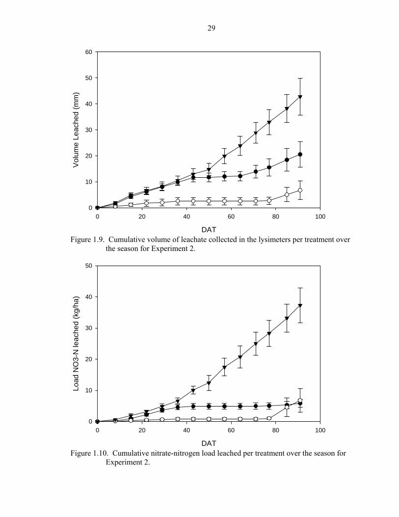
1.9 Cumulative volume of leachate collected in the lysimeters per treatment over the season for Experiment 2. ..........................................................................................29
1.10 Cumulative nitrate-nitrogen load leached per treatment over the season for Experiment 2. ...........................................................................................................29
2.1 A venturi injector schematic showing flow directions and operating principle (adapted from Mazzei Injectors Inc.) .......................................................................44
2.2 Pumphouse hardware layout for Experiment 1 ........................................................47
2.3 Venturi injectors placed across pressure regulators for added pressure differential. ...............................................................................................................47
2.4 Weekly manual injection of fertilizer solution carried out using a peristaltic pump for Experiment 2. ...........................................................................................50

ix
2.5 Cumulative nitrogen rates comparing continuous and manual fertigation treatments in Experiment 2 on sandy soil. ...............................................................51
2.6 Fertigation system for decoupled time-based fertigation and soil moisture-based irrigation. ..................................................................................................................54
4.1 ECH2O dielectric capacitance soil moisture probe (Decagon Devices Inc., Pullman, WA)...........................................................................................................61
4.2 Grid of nine ECH2O probes placed between two actively growing zucchini plants to determine soil moisture distribution for probe placement.........................63
4.3 TDR nest to measure soil moisture for corresponding to mV irrigation threshold set point. ...................................................................................................................64
4.4 Nest of dielectric capacitance probes and tensiometers used to generate the drier points of the soil moisture release curve for the fine sand at PSREU......................66
4.5 Probe grid of 33 dielectric capacitance probes to determine spatial dynamics in the root zone of a mature zucchini crop in plastic mulched bed ..............................67
4.6 Dielectric capacitance probe readings for different spatial positions within the root zone of a plastic mulched crop irrigated using a 475mV set-point. .................68
4.7 Dielectric capacitance probe readings for different spatial positions within the root zone of a plastic mulched crop irrigated using a 525mV set-point. .................69
4.8 Dielectric capacitance probe readings for different spatial positions within the root zone of a plastic mulched crop irrigated using a 475mV set point...................69
4.9 Bivariate plot of TDR and dielectric capacitance probes to obtain a linear relationship between soil moisture and mV .............................................................70
4.10 Soil moisture release curve obtained from in-situ measurements for the fine sand at the Plant Science Research and Education Unit in Citra County.........................71
4.11 Plot of soil moisture release curve obtained from manual tensiometer readings and data obtained from nests of tensiometers and TDRs. ........................................72
4.12 Soil moisture release curve and fitted model derived by ECH2O data and the calibration curve, corrected from nested tensiometer and TDR data. ......................72
4.13 Average soil moisture distribution between two zucchini plants in a plastic mulched bed using soil moisture based drip irrigation (threshold 475 mV). ...........73
4.14 Variability of soil moisture within the zone between two zucchini plants irrigated by soil moisture-based drip irrigation (threshold 475 mV) .......................73

x
4.15 Average soil moisture distribution between too zucchini plants in a plastic mulched bed using soil moisture based drip irrigation (threshold 525 mV) ............74
4.16 Variability of soil moisture within the zone between two zucchini plants irrigated by soil moisture-based drip irrigation (threshold 525 mV) .......................74
4.17 Average soil moisture distribution for the root zone of a mature zucchini plant irrigated by soil moisture-based scheduling (threshold 475 mV). ...........................75
4.18 Soil moisture variability for the root zone of a mature zucchini plant irrigated by soil moisture-based scheduling (threshold 475 mV)................................................75
4.19 Average soil moisture tension for the root zone of a mature zucchini plant irrigated by soil moisture-based scheduling (threshold 475 mV). ...........................76
4.20 Average cross-section profile of soil moisture across the bed with varying distance from drip tape for a mature zucchini crop..................................................77
4.21 Soil moisture time series showing how soil moisture spikes during rainfall events are limited to probes on exterior of bed ........................................................78
4.22 Temperature fluxes within three plastic mulched beds in the fall season of 2005. Thermocouples were buried approximately 15 mm beneath the surface.................80
4.23 Time series of soil moisture in bed I1 to show limited effects of temperature on outer probes that receive little irrigation water. .......................................................81
4.24 Water applications for the three soil moisture-based drip irrigation treatments I1, I2 and I3 on a plastic mulched zucchini crop...........................................................83
4.25 Soil moisture time series showing soil moisture determined by TDR and calculated by dielectric capacitance for soil moisture treatment I1. ........................83
4.26 Soil moisture time series showing soil moisture determined by TDR and calculated by dielectric capacitance for soil moisture treatment I2. ........................84
4.27 Soil moisture time series showing soil moisture determined by TDR and calculated by dielectric capacitance for soil moisture treatment I3 .........................84
A.1 Bypass venturi assembly for fertigation using either a pressure regulator or a control valve. ............................................................................................................99
A.2 Bypass assembly with a booster pump for venturi injection fertigation. ...............100
A.3 Bypass assembly with venturi injector installed across an irrigation pump. .........100
A.4 Automated soil moisture-based irrigation scheduling hardware developed by the University of Florida ..............................................................................................102

xi
A.5 Cumulative water use for ETc and the estimate for soil moisture-based scheduling using the QIC and dielectric probe set to 25 cbar soil moisture ..........104
A.6 Required 4-0-8 liquid fertilizer dilution to achieve IFAS rates when driven by estimated soil moisture-based water application....................................................105
A.7 Step-wise estimated evapotranspiration functions vs. likely actual functions. ......106
B.1 Probe layout and numbering, used to determine soil moisture distribution within the root zone of a mature zucchini plant grown in plastic mulched beds. .............107
B.2 ECH2O probes placed next to drip line, mV output. .............................................108
B.3 ECH2O probes placed perpendicular to drip tape to drip, line mV output. ...........108
B.4 ECH2O probes parallel to and 30 cm from the drip line, mV output. ...................109
B.5 ECH2O probes parallel to and 15 cm from the drip line, mV output. ..................109
B.6 ECH2O probes parallel to and –15 cm from the drip line, mV output. .................110
B.7 ECH2O probes parallel to and –30 cm from the drip line, mV output. .................110
B.8 ECH2O probes perpendicular to and 30 cm from the drip line, mV output. .........111
B.9 ECH2O probes perpendicular to and 15 cm from the drip line, mV output. .........111
B.10 ECH2O probes perpendicular to and -15 cm from the drip line, mV output. ........112

xii
Abstract of Thesis Presented to the Graduate School
of the University of Florida in Partial Fulfillment of the Requirements for the Degree of Master of Engineering
SOIL MOISTURE-BASED IRRIGATION: A SCHEDULING METHOD TO IMPROVE FUTURE RESORCE USE EFFICIENCIES AND PROMOTE
AGRICULTURE SUSTAINABILITY
By
Jonathan Schroder
May 2006
Chair: Rafael Munoz-Carpena Cochair: Michael Dukes Major Department: Agricultural and Biological Engineering
To improve water and nutrient use efficiency, growers need to maintain the soil
water in the crop root zone at optimal levels for plant growth and minimal nutrient
leaching. An automated drip irrigation system has been developed that interfaces a
dielectric capacitance probe to evaluate soil moisture and control irrigation accordingly.
If the soil moisture is below a user-set threshold the scheduled irrigation event is
initiated. If soil moisture is above the threshold, the event is bypassed and water is
conserved. Multiple small volume events are scheduled per day. The aims of this three-
season project were to quantify the water applications and the leached loads of nutrients
for soil moisture-based irrigation and traditional time-based irrigation; to develop a
fertigation methodology that could be integrated with soil moisture-based irrigation; and
to calibrate the soil moisture probe for sandy soils common in Florida, and gain
knowledge on the spatial dynamics of soil moisture within the plastic mulched beds.

xiii
Two experiments were conducted on tomato crops, one on Krome, a calcareous gravely
loam soil in South Florida, and another on a fine sandy soil in North Central Florida.
Replicates of soil moisture-based scheduling and time-based scheduling were applied.
Soil moisture-based scheduling applied 55 to 80% less irrigation water and yielded
Irrigation Water Use Efficiencies (IWUE’s) of 200% to 415% higher than time-based
scheduling. Leachate volumes were 68–74% lower, a 90% reduction of leached NH4-N,
a 75-89% reduction in NO3-N, and an 85% reduction in dissolved and total phosphorous
loads leached, and were obtained by soil moisture-based treatments compared to the time
based treatments. To further improve the system’s nutrient management an automated
fertigation system to be integrated within a soil moisture-based irrigation system was
developed and tested. The system used a venturi injector and provided sufficiently
accurate fertilizer applications to meet the crop nutrient needs throughout the season.
The system is easy to manage and relatively inexpensive. An experiment on a plastic
mulched zucchini crop was conducted to better understand spatial soil moisture
dynamics. This is critical, as the information from the soil moisture probe drives the
irrigation. Soil moisture in a narrow zone of up to 15 cm away from the drip line was
influenced by irrigation events in the fast draining sand soil. Soil moisture tensions were
found to increase rapidly beyond 8% soil moisture by volume. Temperature, and rainfall
showed very little effect on output readings of the dielectric capacitance probe, but
salinity effects could be significant and need to be calculated. The system has proved to
be successful at improving water and nutrient use efficiencies, and shows potential for
improved coexistence of vegetable production agriculture with environmental systems.

1
CHAPTER 1 INTRODUCTION
For the purpose of motivation of research this first chapter will briefly introduce
water management issues pertaining particularly to agriculture in Florida. Focus will be
given to areas where water management challenges have prompted agriculture to advance
its systems and become more competitive and sustainable.
Rationale
The Everglades and associated costal ecosystems of South Florida are unique and
highly valued ecosystems. One of the world’s largest water management systems has
been developed in South Florida over the past 50 years to provide flood control, urban
and agricultural water supply, and drainage of land for development. However this
system has inadvertently caused extensive degradation of the South Florida ecosystems
and elimination of whole classes of ecosystems. The hydrodynamics and water quality in
Everglades National Park and adjacent lands are now being restored in accordance with
the Comprehensive Everglades Restoration Plan (CERP). CERP
authorizes modifications of the existing surface water management system, so as to re-
establish historic freshwater flows that restore more natural hydro-patterns in the Park
and contribute to ecosystem restoration. Part of CERP’s mission is also to protect the
water resources in Central and Southern Florida by balancing and improving water
quality and supply. Lack of knowledge about the hydrological system and its effects on
crops, local and regional flow, and chemical transport patterns are all major concerns for
all stakeholders in the area (Muñoz-Carpena, 2004). As such, farmers in the area have

2
taken a key role in promoting the need for scientific investigation into the possible impact
of CERP on the sustainability of agriculture in South Florida.
To understand the scale of the industry that is being impacted by the need for
environmental compatibility one needs to look at the extent of agriculture in Florida.
Florida ranks second among the states in fresh market vegetable production on the basis
of area cultivated (9.6%) and in value (13%) of the crops grown. Tomato production
accounted for over 30% of the state’s total production in value in 2001-2002. According
to the National Resources Conservation Service (1995), Dade County produces roughly a
quarter of the state’s tomatoes. Higher yields than more northern growing areas, and the
ability to produce a crop during the winter season when other regions are inactive, have
helped establish this region’s importance in the tomato market. The Miami-Dade County
vegetable crops industry also employs over 6000 people, and has a $491 million impact
on the state economy.
Florida tomato growers are at a competitive disadvantage due to off-shore
competition from countries where labor is considerably cheaper than in the United States.
This disadvantage is even greater with the phase out of methyl-bromide in the U.S, but
not in other developing countries. Apart from environmental benefits, the vegetable
industry in Florida is hugely in need of methodologies that improve resource use and
decrease operating costs.
Water is a vital resource and is a driving force for much of crop production. With
its large contribution to industry in Florida, agricultural self-supply accounts for 35% of
fresh ground water withdrawals, and 60% of fresh surface water withdrawals, which
makes it the largest component of freshwater use in Florida (Marella, 1999). Overall,

3
82% of the farms in the Miami-Dade County have irrigation systems. The primary use of
this water is irrigation to supplement rainfall during dry crop periods (Muñoz-Carpena et
al., 2004). The high yields of the Biscayne Aquifer were originally attractive for growers
and have lead to the general perception among growers that water is not a limiting factor.
But as urban pressure in the Miami-Dade County area increases, water could become a
more scarce resource (Muñoz-Carpena et al., 2002). Despite the potential shortages,
over-irrigation is a problem in the area and may be explained by the low water holding
capacity and high permeability of Florida’s sandy soils, and especially the gravelly soils
found in the south Miami-Dade County agricultural area. Analysis shows that irrigation
efficiency is highly sensitive to both soil texture and irrigation volume. Over irrigation
can also be attributed to inadequate irrigation scheduling (Muñoz-Carpena et al., 2004).
Traditional irrigation based on low frequency and high volumes usually results in
inefficient water use. With this type of irrigation, a substantial volume of the applied
water percolates quickly to the shallow groundwater, potentially carrying with it nutrients
and other agrochemicals applied to the soil (Muñoz-Carpena et al., 2003a).
For some important reasons, drip irrigation of raised beds covered with plastic
mulch is the most suited form of micro irrigation for high value vegetable production. Its
slower more precise application of water is suitable to easily drained soils and one of the
major benefits of drip irrigation is the capacity to conserve water and fertilizer compared
to overhead sprinklers and subirrigation. Drip irrigation also helps reduce foliar disease
incidence compared to overhead sprinkler systems, which wet the plant foliage. By
maintaining drier plants drip irrigation reduces susceptibility to outbreaks of bacteria and
fungal diseases, and reduces the need for bactericides and fungicides (Hochmuth and

4
Smajstrla, 1998). Drip irrigation provides for precise timing and application of nutrients
and certain pesticides in vegetable production. Fertilizers can be prescription-applied
during the season in amounts that the crop needs and at particular times when those
nutrients are needed. These small, controlled applications of fertilizer under plastic
mulch not only save fertilizer, but also have the potential to reduce groundwater pollution
due to fertilizer leaching from heavy rainstorms or irrigation.
Drip irrigation however has become the standard for plastic mulched raised bed
vegetable production, and no longer gives any benefits over competitors. Furthermore,
the design and implementation of a good irrigation system requires good scheduling for it
to operate efficiently. The University of Florida’s Institute of Food and Agricultural
Sciences, a leader in developing best management practices, recommends scheduling
according to crop evapotranspiration requirements combined with soil moisture
monitoring. A methodology of scheduling has recently been developed to automatically
schedule water according to soil moisture status. Preliminary tests have shown the
system has potential for large savings in water application from traditional methods of
irrigation scheduling.
More and more, water conservation appears on top priority lists for projecting,
planning and managing future water needs, not just in South Florida, but statewide and
globally as well (Anon, 2003).
The following Chapters will introduce and discuss an automated drip irrigation
system and management practices that have been developed and tested by the University
of Florida. Different aspects of the system will be analyzed, namely the system
configuration and hardware, the system’s ability to conserve water and reduce leaching

5
with results from field trials, and the potential of integrating soil moisture based
scheduling with continuous fertigation. Although these studies have focused on a
specific hardware technology, it must be strongly emphasized that it is not the specific
technology that is of highest importance, but the methodologies presented here within.
The potential of the system lies within the methodology; the technologies are important
for optimization of the method.
Objectives
Chapter 2
1. To test and mange water and fertilizer application with the automated soil moisture based irrigation system
2. To quantify the load of nutrients being leached from the root zone of the crop for different irrigation scheduling methods to determine the effectiveness of the proposed system in reducing leaching loses
3. To demonstrate that with proper management that yields can be maintained while reducing water and nutrient application from local grower standards
Chapter 3
4. To evaluate the potential and effectiveness of integrating soil moisture based irrigation scheduling and automatic continuous fertigation
Chapter 4
5. To better understand soil moisture distribution within plastic mulched beds and its effects on probe placement for soil moisture based irrigation
6. To calibrate the soil moisture probe used with the UF developed automated soil moisture based system for the fine sand soils at local research site
Chapter 5
7. To hi-light potential issues for future research within this field.

6
CHAPTER 2 SOIL MOISTURE BASED DRIP IRRIGATION FOR IMPROVED WATER USE
EFFICIENCY AND REDUCED LEACHING ON TOMATOES
Introduction
Florida tomato growers are at a competitive disadvantage due to off-shore
competition from countries where labor is cheaper than in the United states (Munoz-
Carpena et.al., 2005). Improving irrigation efficiency can contribute to reducing
production costs of vegetables and make the industry more competitive and sustainable.
Through proper irrigation, average yields can be maintained or increased (Shae, et al.,
1999) while minimizing environmental impacts caused by excess water application and
subsequent agrichemical leaching. Tomatoes are typically grown in raised beds with
plastic mulch and drip irrigation. Although this method has the potential to be very
efficient, over-irrigation is a common occurrence in Florida due to inadequate irrigation
scheduling and low soil water holding capacity of soils commonly used for agriculture.
Traditional irrigation of applying large volumes of water at low frequencies (a few times
per week) results in a large portion of the irrigated water percolating quickly through the
root zone to the shallow groundwater, potentially carrying with it nutrients and other
agrochemicals in the soil. In addition, excess water in the root zone can reduce tomato
yields (Wang et al., 2004).
Recent technological advances have made low-cost soil water sensors available for
efficient and automatic operation of irrigation systems (Dukes and Muñoz-Carpena,
2005). Automation of irrigation systems based on soil moisture sensors may improve

7
water use efficiency by maintaining soil moisture at optimum levels in coarse soils (sands
and gravels) rather than a cycle of very wet to very dry as a result of typical low
frequency high volume irrigation. This is particularly critical in Florida’s sand and gravel
soils where available soil moisture is typically 6-8% by volume or less (Dukes et al.,
2003).
Soil moisture probes can be installed at representative points in an agricultural field
to provide repeated moisture readings over time for irrigation scheduling and
management. The target soil water status is usually set in terms of soil tension (or matric
potential expressed in kPa or cbar), or volumetric moisture content. Care needs to be
taken when using these soil moisture sensor devices in coarse soils, as most devices
require good contact with the soil matrix, which is difficult coarse soils (Dukes and
Munoz-Carpena, 2005). In addition soil moisture sensing devices need to be able to
capture fast soil water changes typical to coarse soils. Tensiometers have been widely
used in soil moisture based scheduling in various applications such as tomato production
(Clark et al, 1994; Smajstrla and Locascio, 1994), blackcurrent production (Hoppula and
Salo, 2005), and rice (Kukal, et al., 2005). Due to their direct reading of soil matrix
potential and thus plant water stress, tensiometers provide good scheduling applications.
Tensiometers however need to be carefully maintained (e.g. refilled) and the ceramic cup
has the potential to loose contact with coarse soils, requiring reinstallation. Dielectric
probes however need little maintenance and can be accurate without soil specific
calibrations, although soil-specific calibration increases accuracy, and is recommended
on certain soils (Munoz-Carpena, 2004). A drawback of some dielectric probes is the
cost due to the complex electronics.

8
Soil moisture based scheduling has resulted in water savings on coarse soils in
Florida. Smajstrla and Locascio (1996) reported reductions of irrigation of 40 to 50%
compared to local practices without affecting yield using switching tensiometers to
irrigate tomatoes on fine sands in Florida. Scheduling according to soil matric potential
measuring devices achieved a 70% reduction in water applications against time based
practices for tomato grown on a calcareous soil in South Florida compared to local
grower practices was reported by Muñoz-Carpena et al., (2005). The methodology of
using soil moisture based scheduling has been used successfully on other crops and
applications such as citrus (Fares and Alva, 2000), potatoes (Shae et al., 1999) and
(Shock et al., 1998), onions (Shock et al., 2000), and for the automatic irrigation of urban
landscapes (Qualls et al., 2001).
Corresponding reductions in nutrient leaching loads due to reduced water
applications are expected. Hebbar et al. (2003) found improved fertilizer use efficiencies
with all drip irrigated and fertigated treatments over furrow irrigation, as well as reduced
NO3-N leaching from soil analysis at varying depths. Drip irrigation and fertilizer
applied through fertigation, combined with soil moisture based scheduling has high
potential for reducing leaching of nutrients, but little quantification of the loads leached
have be reported.
The objective of this project were to determine the effect of the soil moisture-based
irrigation scheduling applied to plastic mulched tomatoes grown on two soil types and
seasons. The soil moisture based-irrigation scheduling was compared to traditional
time-based scheduling. Different dependant variables were studied to determine the
effect of the independent variable (irrigation scheduling method). The different variables

9
that were studied were 1) water application by treatment, 2) yield and water use
efficiency for each treatment, 3) volume of leachate passing through the root zone as a
result of different treatment water applications, and 4) the load of nutrients in the leachate
lost from the root zone corresponding to each treatment.
Methods and Materials
Two field trials were conducted on plastic mulched tomato crops using the soil
moisture based drip irrigation system. The first experiment was conducted during the
2004/2005 winter cropping season on gravelly loam soil in Homestead, Miami-Dade
County in South Florida. The second experiment was conducted during the 2005 spring
cropping season on sandy soils in Marion County, North Central Florida.
Soil Characteristics
The field site of the first experiment was at the Tropical Research and Education
Center (TREC) in Homestead, Miami-Dade County. The region is dominated by three
calcareous soils, namely Krome, Chekika, and Marl (Munoz-Carpena et al., 2002). The
soil at TREC is Krome, a calcareous soil artificially made by rock-ploughing the top
layer of the limestone coral bedrock. It is a bimodal soil and has 51% gravel particles
and the remainder is loam texture. The highly permeable gravel component the soil
presents soil water management challenges to growers in the area. A large portion of the
soil water (approx. 50%) can easily be leached during regular water applications, due to
the low water holding potential of the gravel component of the soil.
The second field site was at the Plant Research and Education Unit (PSREU) in
Marion County, on sandy soils. Buster (1979) classified the soil at the PSREU research
site as a Candler sand and Tavares sand. These soil types contain 97% sand-sized
particles and have a field capacity of 5.0% to 7.5% by volume in the upper 100 cm of the
10
soil profile (Carlise et al., 1978). Like the Krome soil in South Florida, the sandy soils of
this region are highly permeable and also have a low water holding capacity and high
potential for leaching.
Experimental Design
Tomatoes were grown according to local agronomic practices in each region. The
field in Experiment 1 had sorghum sudangrass grown as cover crops prior to the
cultivation and the tomato-cropping season. The tomato seedlings of the cultivar, ‘FL
47’, were transplanted on the 15th of October 2004 (Experiment 1), and the 5th of April
2005 (Experiment 2) into raised black plastic mulched beds. The beds were spaced 1.83
m apart, center-to-center, and seedlings were planted in one row per bed with plants
spaced 0.46 m apart. Dual drip lines under the plastic mulch were used to supply
irrigation water to the crop on the gravelly loam soil (Experiment 1), and single lines
were used for the sandy soil (Experiment 2). Dual lines were employed on Experiment 1
as the gravelly loam soil was only 35-45 cm deep and the wider wetting area would
provide a larger soil water storage volume, which is common horticultural practice.
Field layout
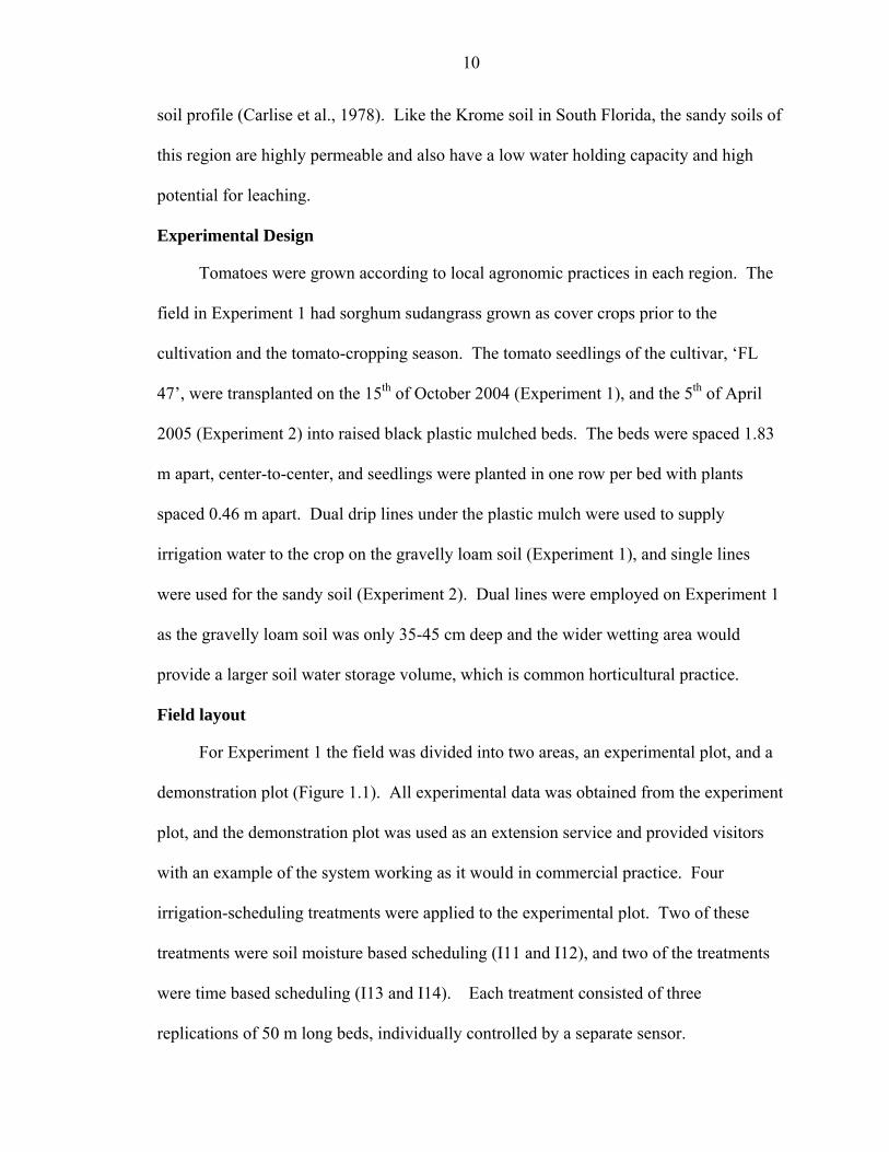
For Experiment 1 the field was divided into two areas, an experimental plot, and a
demonstration plot (Figure 1.1). All experimental data was obtained from the experiment
plot, and the demonstration plot was used as an extension service and provided visitors
with an example of the system working as it would in commercial practice. Four
irrigation-scheduling treatments were applied to the experimental plot. Two of these
treatments were soil moisture based scheduling (I11 and I12), and two of the treatments
were time based scheduling (I13 and I14). Each treatment consisted of three
replications of 50 m long beds, individually controlled by a separate sensor.

11
To reduce wiring treatments were not spatially randomized and control points could
be kept close together in the field and supplied by a single multiple station cable. The
demonstration plot consisted of two treatments, a soil moisture based treatment I12, and
the local grower time based treatment I14. Figure 1.1, shows the field layout.
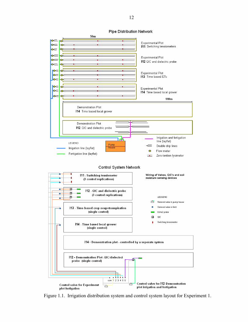
For Experiment 2 on the gravelly loam soil, a randomized complete block design
was used. Three irrigation treatments consisted of two soil moisture-based schedules,
and the third treatment was a time-based local grower schedule. Each treatment was
replicated four times (four 15 m beds) and a common valve and soil moisture probe
controlled all four replicates. Treatments I21 and I22 were soil moisture-based
treatments and I23 was a time-based treatment, similar to grower practices (Table 1.1).
Table 1.1. Scheduling treatments applied to two irrigation experiments on tomato crops.
The field layout and treatments can be seen in Figure 2. A single drip tape supplied
the irrigation water and a second line supplied the fertilizer. For treatments I22 and I23
these two lines were placed next to each other in the middle of the bed at the surface
under the plastic mulch. For treatment I21, the irrigation line was buried 15 cm beneath
the surface and 15 cm offset from the fertigation line, which was at the surface. Plats
were transplanted 10 cm away from the drip lines. In treatment I21 this was 10cm from
the fertilizer line at the surface.
Experiment Treatment Scheduling Method Device/practice
I11 Soil moisture-based Switching tensiometersI12 Soil moisture-based ECH2O dielectric probeI13 time-based ETc based on historical weather dataI14 time-based Local grower practice
I21 Soil moisture-based ECH2O dielectric probeI22 Soil moisture-based ECH2O dielectric probeI23 Time-based Local grower practice
1
2
12
Figure 1.1. Irrigation distribution system and control system layout for Experiment 1.
13
Figure 1.2. Field layout and irrigation treatments for Experiment 2.

14
Irrigation control and data capture hardware
The soil moisture-based treatments applied water during preset events depending
on soil moisture status. An irrigation timer was used to preset sub-daily irrigation events.
When it was time for an event to occur the soil moisture sensor was queried. If soil
moisture was below a set threshold the soil moisture sensor would allow a set event to
occur. If soil moisture was above the threshold set point, the event would be bypassed.
For Experiment 1 treatments I11 and I12 used switching tensiometers (LT-RA, Irrometer
Co., Inc., CA), and dielectric capacitance probes (ECH2O, Decagon Devices Inc.,
Pullman, WA) respectively. The switching tensiometer irrigation set point was set at a
soil matric potential of 25 cbar. The ECH2O probes were interfaced with an irrigation
timer by a quantified irrigation controller (QIC) developed by the University of Florida
Agricultural and Biological Engineering Department (Dukes and Munoz-Carpena, 2005).
The irrigation threshold for the QIC was set to 400mV, which corresponded to a soil
matric potential of approximately 25 cbar for the gravelly soil and dielectric probe.
Treatments I13 and I14 were time based with I13 derived from historic weather data and
IFAS recommended crop coefficients (Simonne et al., 2004), and I14 following local
grower practices, which corresponded to 1 hour of irrigation per day for the system (4
mm/day).
For Experiment 2 treatments I21 and I22 used dielectric, capacitance probes
(ECH2O, Decagon Devices Inc., Pullman, WA) interfaced with an irrigation timer using
QICs (Munoz-Carpena and Dukes, 2005). The irrigation threshold for the QICs was 500
mV, which corresponds to soil moisture content by volume of roughly 10-13 % for the
sandy soil using dielectric capacitance probes. Treatment I21 had its irrigation drip-tape
buried in the soil 15 cm beneath the surface of the bed, and its fertigation line on the

15
surface. Treatment I23 was the local grower practice time based treatment, and irrigated
once a day for 1 hour (2.1 mm/day) for the first 45 days after transplanting, and 2 hours
(4.2 mm/day) for the remaining 40 days in the season.
Soil moisture based scheduling with an automated system can apply water in two
different procedures. The soil moisture probes can continuously read the soil moisture
status and initiate irrigation whenever the level gets below a threshold, and switch the
irrigation off when once the profile has been sufficiently wetted which is an “on-demand”
technique (Dukes and Muñoz-Carpena, 2005). This technique has negative design
complications. The maximum flow rate of the system is not known, as the time at which
irrigation events occur during a day is dynamic, and there could be many valves open at
once or none. To accommodate the possibility that all the soil moisture treatment valves
could be open at once the system pipe network would have use large diameter pipes.
This would be particularly impractical in commercial systems where larger areas are
irrigated. As such, a fixed schedule of sub-daily events was employed where the soil
moisture sensor control system could bypass these timed events if soil moisture was
adequate (Dukes and Muñoz-Carpena, 2005).
For Experiment 1 four events of 12 minutes per event were employed per day.
This corresponded to maximum daily needs for the season (2.5 mm/day) calculated from
historical weather data (ETo = 2.79 mm/day) and crop coefficients (Kcmax = 0.9).
Experiment 2 was conducted during the following spring-summer season when warmer
temperatures increase crop water needs. As such five events per day were chosen. For
the beginning of the season each event was 12 minutes long. After 48 days the event
length was extended to 24 minutes (4.1 mm/day), which corresponded to the maximum

16
daily water requirement for a tomato crop in the area, and was derived from historical
weather data (ETo = 4.57mm/day) and crop evapotranspiration coefficients (Kcmax = 0.9).
Crop coefficients and historical weather data were obtained from (Simonne et al., 2004).
A schedule was programmed into an irrigation timer. The schedule consisted of 4
events per day (Experiment 1), and five events per day (Experiment 2). Each of the 4
events in Experiment 1 was 12 minutes long, and the 5 events in Experiment 2 were 12
minutes long for the first 45 days after transplant and 24 minutes long for the remaining
40 days. The soil moisture probes then either allowed or bypassed a prescheduled event
according to in-field soil moisture status, and a set threshold. The sub-daily events were
staggered and spread out through the day so that only one treatment was irrigated, if
needed, at a time. As a result of this scheduling set up, water is still delivered to the crop
as determined by the soil moisture probes, but the maximum flow rates are explicit and
reduced. The system specifications for Experiments 1 and 2 are presented in Table 1.2
and 1.3.
Water applications per treatment for Experiment 2, and per replication (individual
beds) within treatments for Experiment 1 were manually recorded from positive
displacement flowmeters (V100 1.6 cm diameter bore with pulse output, AMCO Water
Metering Systems Inc., Ocala, FL). In addition to manual readings on a weekly basis, the
flowmeters contained transducers that signaled a switch closure every 18.9 L. The switch
closures were recorded by data loggers (HOBO event logger, Onset Computer Corp. Inc.,
Bourne, MA) and provided continuous data of water and fertigation application times,
which were downloaded once a week. This data could be used to determine which events
had occurred and which were bypassed.
17
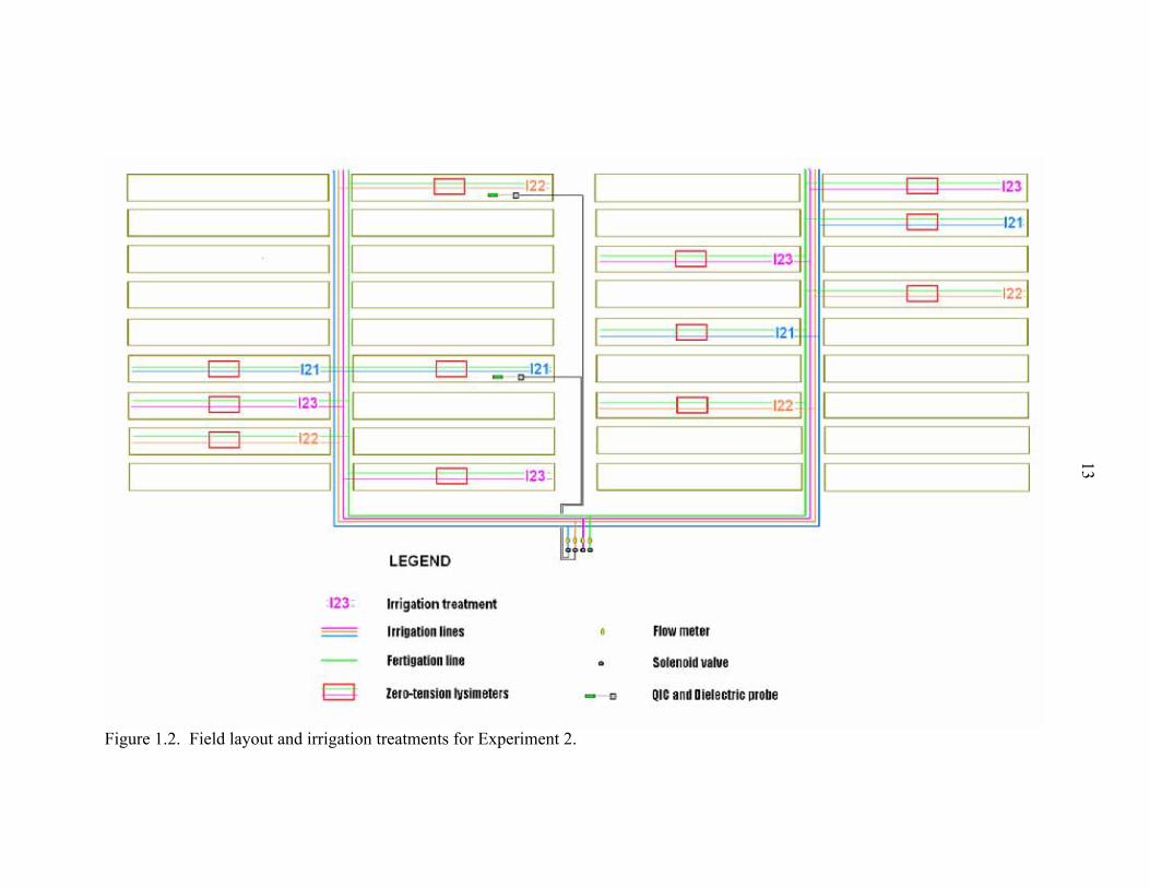
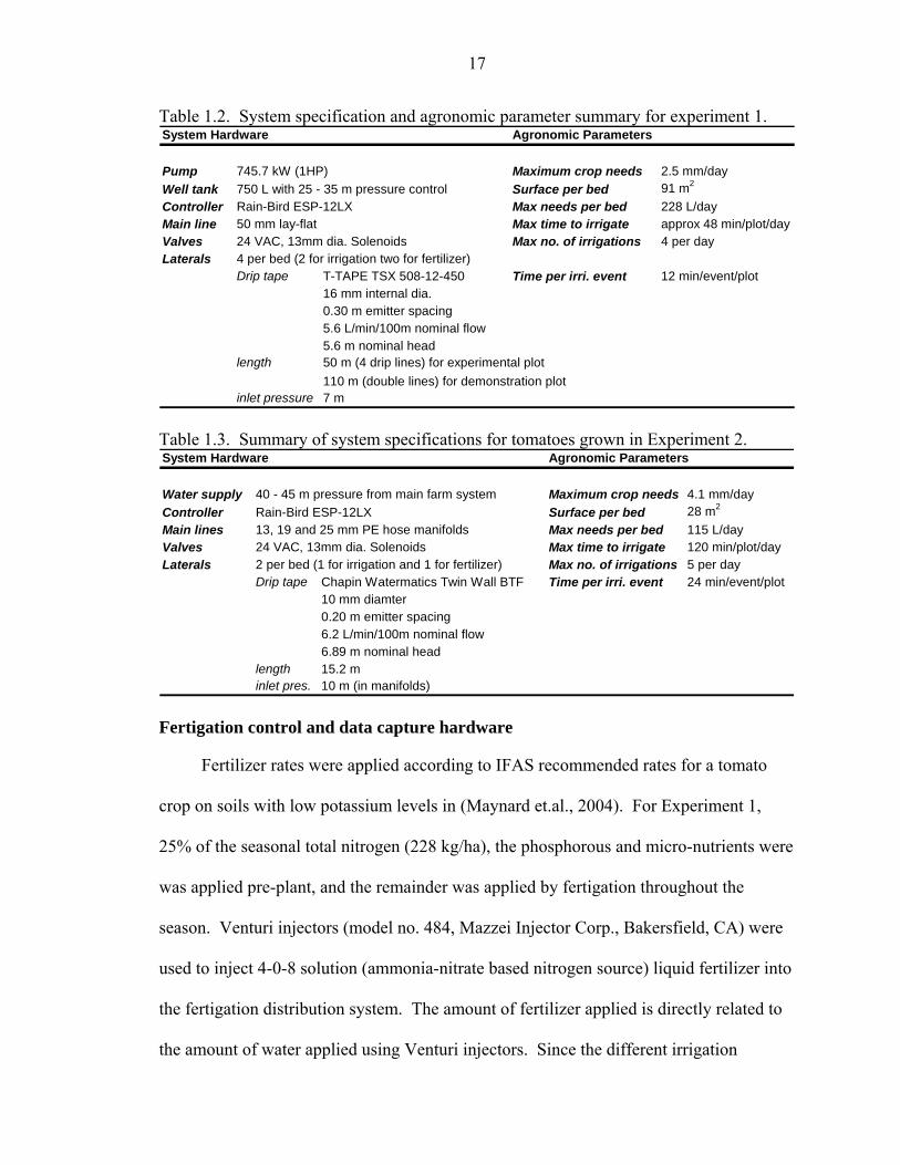
Table 1.2. System specification and agronomic parameter summary for experiment 1.
Table 1.3. Summary of system specifications for tomatoes grown in Experiment 2.
Fertigation control and data capture hardware
Fertilizer rates were applied according to IFAS recommended rates for a tomato
crop on soils with low potassium levels in (Maynard et.al., 2004). For Experiment 1,
25% of the seasonal total nitrogen (228 kg/ha), the phosphorous and micro-nutrients were
was applied pre-plant, and the remainder was applied by fertigation throughout the
season. Venturi injectors (model no. 484, Mazzei Injector Corp., Bakersfield, CA) were
used to inject 4-0-8 solution (ammonia-nitrate based nitrogen source) liquid fertilizer into
the fertigation distribution system. The amount of fertilizer applied is directly related to
the amount of water applied using Venturi injectors. Since the different irrigation
System Hardware Agronomic Parameters
Pump 745.7 kW (1HP) Maximum crop needs 2.5 mm/dayWell tank 750 L with 25 - 35 m pressure control Surface per bed 91 m2
Controller Rain-Bird ESP-12LX Max needs per bed 228 L/dayMain line 50 mm lay-flat Max time to irrigate approx 48 min/plot/dayValves 24 VAC, 13mm dia. Solenoids Max no. of irrigations 4 per dayLaterals 4 per bed (2 for irrigation two for fertilizer)
Drip tape T-TAPE TSX 508-12-450 Time per irri. event 12 min/event/plot16 mm internal dia.0.30 m emitter spacing5.6 L/min/100m nominal flow5.6 m nominal head
length 50 m (4 drip lines) for experimental plot110 m (double lines) for demonstration plot
inlet pressure 7 m
System Hardware Agronomic Parameters
Water supply 40 - 45 m pressure from main farm system Maximum crop needs 4.1 mm/dayController Rain-Bird ESP-12LX Surface per bed 28 m2
Main lines 13, 19 and 25 mm PE hose manifolds Max needs per bed 115 L/dayValves 24 VAC, 13mm dia. Solenoids Max time to irrigate 120 min/plot/dayLaterals 2 per bed (1 for irrigation and 1 for fertilizer) Max no. of irrigations 5 per day
Drip tape Chapin Watermatics Twin Wall BTF Time per irri. event 24 min/event/plot10 mm diamter0.20 m emitter spacing6.2 L/min/100m nominal flow6.89 m nominal head
length 15.2 m inlet pres. 10 m (in manifolds)

18
treatments were expected to apply different amounts of water, the water and fertigation
applications were separated so that each treatment received a variable amount of water,
but a common amount of fertilizer. A separate pipe distribution system was thus used to
fertigate all treatments for the experimental plot. Fertilizer was injected directly into the
irrigation system of the demonstration plot as would be done in a commercial practice.
The venturi injectors were calibrated before the start of the experiment, and were found
to provide consistent injection rates with those specified by the manufacturer, and yet
were low cost and low maintenance. Three venturies were used in Experiment 1, two to
inject fertilizer into the experimental plot fertigation system, and one venturi injected
fertilizer into the demonstration plots irrigation system. The calibration yielded an
average injection rate of 0.90 L/min with a standard deviation of 0.08 L/min.
For Experiment 2 phosphorous fertilizer was broadcast at 110 kg/ha prior to
bedding, along with a blanket of micronutrients. Nitrogen, potassium and magnesium
were all applied through fertigation once per week and none was applied preplant.
Calcium nitrate was the source of nitrogen and a total of 220 kg/ha of N was applied
through the season. Potassium as supplied in the form of Muriate of Potash (KCl) and
250 kg/ha of K was given for the season. Epsom salts applied provided the crop with
12.4 kg/ha of Mg for the season. Injection of the fertilizer in solution was carried out
manually once a week with a peristaltic pump (Experiment 2).
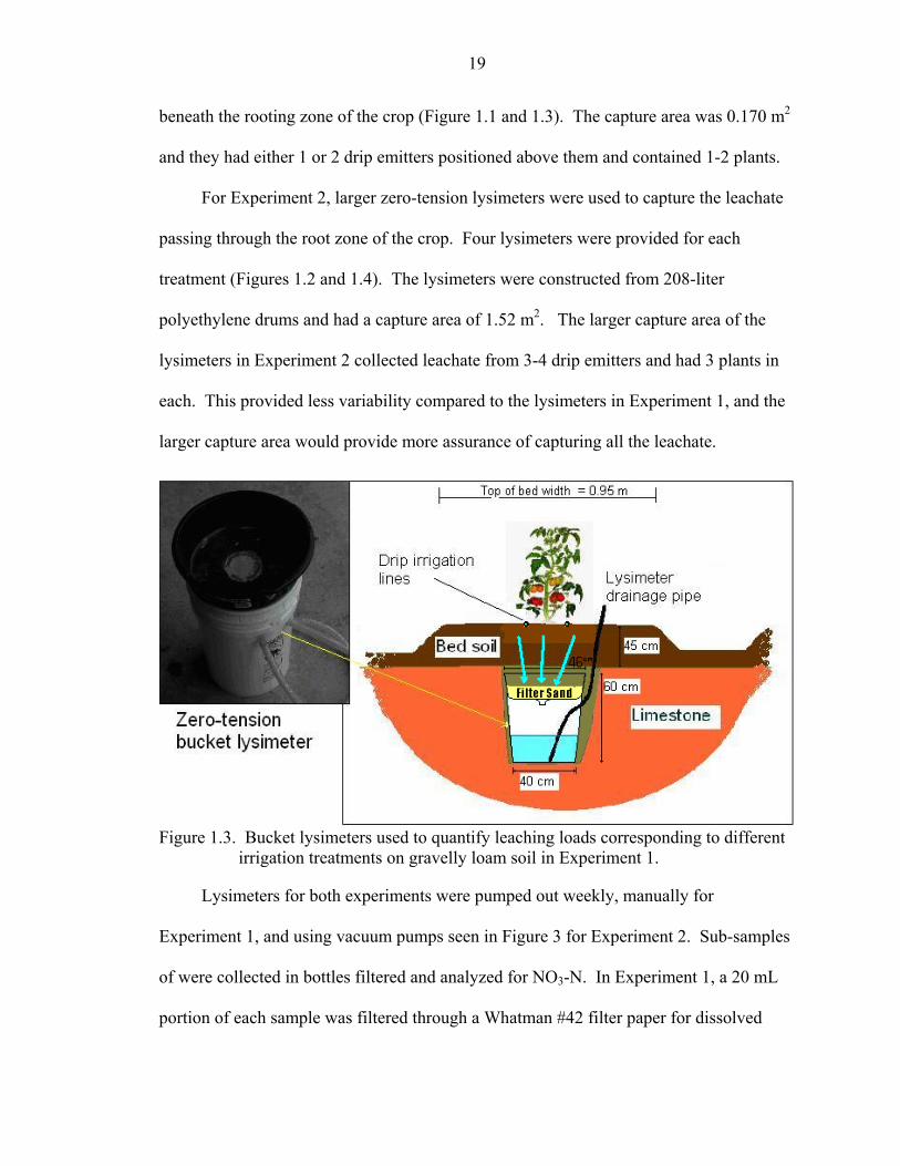
To quantify the volume and loads of nutrients leached associated with each
irrigation treatment, zero-tension lysimeters were installed into the fields. For
Experiment 1 seven zero-tension bucket lysimeters per treatment were buried directly
19
beneath the rooting zone of the crop (Figure 1.1 and 1.3). The capture area was 0.170 m2
and they had either 1 or 2 drip emitters positioned above them and contained 1-2 plants.
For Experiment 2, larger zero-tension lysimeters were used to capture the leachate
passing through the root zone of the crop. Four lysimeters were provided for each
treatment (Figures 1.2 and 1.4). The lysimeters were constructed from 208-liter
polyethylene drums and had a capture area of 1.52 m2. The larger capture area of the
lysimeters in Experiment 2 collected leachate from 3-4 drip emitters and had 3 plants in
each. This provided less variability compared to the lysimeters in Experiment 1, and the
larger capture area would provide more assurance of capturing all the leachate.
Figure 1.3. Bucket lysimeters used to quantify leaching loads corresponding to different irrigation treatments on gravelly loam soil in Experiment 1.
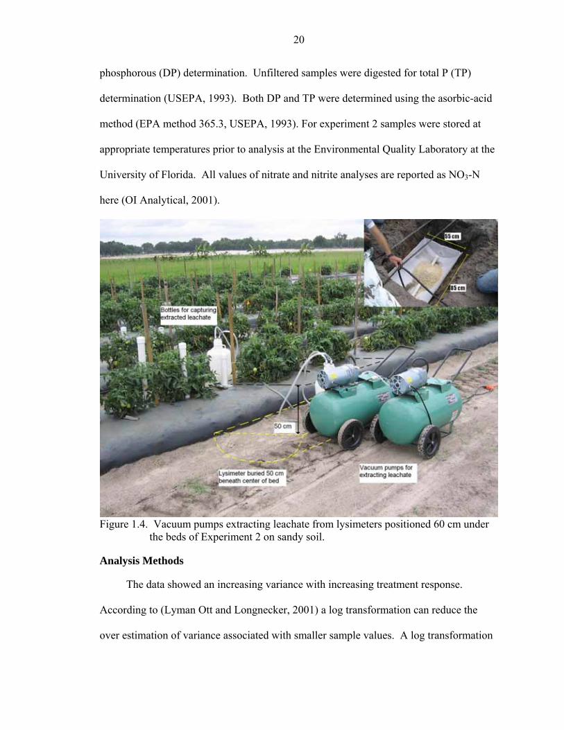
Lysimeters for both experiments were pumped out weekly, manually for
Experiment 1, and using vacuum pumps seen in Figure 3 for Experiment 2. Sub-samples
of were collected in bottles filtered and analyzed for NO3-N. In Experiment 1, a 20 mL
portion of each sample was filtered through a Whatman #42 filter paper for dissolved
20
phosphorous (DP) determination. Unfiltered samples were digested for total P (TP)
determination (USEPA, 1993). Both DP and TP were determined using the asorbic-acid
method (EPA method 365.3, USEPA, 1993). For experiment 2 samples were stored at
appropriate temperatures prior to analysis at the Environmental Quality Laboratory at the
University of Florida. All values of nitrate and nitrite analyses are reported as NO3-N
here (OI Analytical, 2001).
Figure 1.4. Vacuum pumps extracting leachate from lysimeters positioned 60 cm under the beds of Experiment 2 on sandy soil.
Analysis Methods
The data showed an increasing variance with increasing treatment response.
According to (Lyman Ott and Longnecker, 2001) a log transformation can reduce the
over estimation of variance associated with smaller sample values. A log transformation
21
was applied to the dependent variables before statistical analyses were conducted. All
dependent variables were analyzed using one-way ANOVA tests and their means were
compared for treatment effect using the Tukey-Kramer HSD (Honestly Significant
Difference) test. This test is an exact alpha-level test if the sample sizes are the same and
conservative if the sample sizes are different (Hayter 1984). Comparisons were made at
the 95% confidence level. The tests were carried out using JMP Version 5.1 software
(Lehman et al., 2004).
The independent variable was irrigation treatment and the dependent variables were
yield, irrigation water use efficiency, volume leached and load of nutrient leached. Crop
evapotranspiration (ETc) for the seasons was estimated by multiplying reference
evapotranspiration (Eto - calculated from weather data collected at the sites) by crop
coefficients (Kc) presented by Brouwer and Heibloem (1986) that had been adjusted for
plastic mulch field conditions by a reduction factor of 35% determined by (Haddadin and
Ghawi, 1983). According to Howell (2002) the irrigation water use efficiency (IWUE in
kg/m3) is calculated as the increase in yield due to irrigation divided by the irrigation
water. This is shown in Equation 1.
IWUE = (Y-Yd)/(IRR*1000) [1]
Where Y is the total marketable yield (kg/ha)
Yd is the total marketable dryland or non-irrigated yield
IRR is the applied irrigation water (mm)
The non-irrigated yield is assumed to be approximately zero for plastic mulched
tomatoes in Florida. Yields were the sum of two crop harvests for both experiments. The
first harvest of Experiment 1 was on the 13th of January 2005 and the second on the 26th

22
of January 2005. Harvests were from 5 m sections of the beds. The first harvest of
Experiment 2 occurred on the 16th of June 2005, and the second harvest was on the 29th
of June 2005. Harvests of the tomatoes for Experiment 2 occurred from 6 m sections of
the beds. The final marketable yields consisted of XL, L and M fruit as graded according
to the Florida Tomato Committee standards, from the two harvests for each experiment.
Results and Discussion
Results will be presented for each experiment, and comparisons and trends between
the two will then be highlighted and discussed to establish trends and draw conclusions.
Experiment 1: Calcareous gravelly soil
The analysis of treatment effects starts on the 29th of October 2004 when irrigation
treatments were put into effect, and ignores the first two weeks of establishment irrigation
that was common to all treatments. Water application over the season for each treatment
are presented in Figure 1.5, along with estimates of crop evapotranspiration (ETc)
estimated from plastic mulch adjusted crop coefficients. As can be seen the water
application for the soil moisture-based treatments matched crop water needs much more
closely than the time-based treatments, and did not over apply water (Table 1.4).
Table 1.4. Water application, yield, and irrigation water use efficiency (IWUE) averages
for each treatment in Experiment 1 on calcareous gravelly soil. † Different letters depict statistically different means for P ≤ 0.05 (Tukey-Kramer method) [z] Total water per treatment includes the hour per day of establishment irrigation which was treatment independent
Total Water applied [z] Water by treatment Yield IWUEmm mm kg/ha kg/m 3 water
I11 (tensiometer) 169 (± 13) 118 a 49955 a 30 aI12 (Dielectric probe) 101 (± 30) 50 a 40168 a 40 bI13 (time based -ETc) 370 (± 8) 319 b 42191 a 11 cI14 (time based -local grower) 570 (± 90) 519 c 45497 a 8 c
Treatment

23
Figure 1.5. Graph of cumulative season water application for the four irrigation treatments applied to the gravely loam soils of Experiment 1. Error bars represent one standard deviation.
Significant differences were found for average water applications between the soil
moisture-based treatments and time-based treatments. Scheduling according to the crop
growth curve I13 applied less water than the constant rate of I14 through the season. The
treatment employing switching tensiometers (I11) provided 71% water savings over the
time-based treatment (I14), and the dielectric probe and QIC system (I12) achieved 83%
savings over I14. The dielectric probe and QIC hardware required less maintenance and
labor than the switching tensiometers. The tensiometers had to be refilled on a weekly
basis due to breakage of the water column and loss of connection with the soil water in
the coarse textured soil. This is a common problem associated with tensiometers in
DAT
0 20 40 60 80 100
Wat
er a
pplie
d (m
m)
0
50
100
150
200
250
300
350
400
450
500
550
600
650
700
I11 (switching tensiometer)I12 (dielectric probe)I13 (ETc)I14 (time based - local grower)ETc

24
coarse soils. The dielectric probe and QIC were essentially maintenance free and worked
reliably throughout the season once the threshold had been set at the beginning of the
season.
Treatment effect had no significant difference on total marketable yields. Water
use efficiencies followed applied water trends, with the soil moisture based treatments
I11 and I12 using water more efficiently at 30 and 40 kg/m3 respectively, than the
historical weather time-based and local grower time-based treatments I13 and I14 which
yielded only 11 and 8 kg/m3 of water, respectively. The average nutrient leaching data
by treatments obtained from the lysimeters are summarized in Table 1.5.
Table 1.5. Nutrient leaching data obtained from lysimeters in Experiment 1.
† Different letters depict statistically different means for P ≤ 0.05 (Tukey-Kramer HSD method)
The volume leached correlated with water application volumes by treatment, with
low water applications of I11 and I12 having lower volumes of leachate than I13 and I14
(Figure 1.6). Correspondingly the ammonia-nitrogen load, dissolved phosphorous (DP)
load, and total phosphorous (TP) load all were all significantly reduced for the soil
moisture based treatments I11 and I12 over the two time-based treatments I13 and I14.
Phosphorous leaching was analyzed in this experiment due to its present
importance in the Miami-Dade County, and to determine the potential of the system to
reduce loading and help with the concerted effort to control phosphorous levels in the
Everglades and surrounding areas. The soil moisture-based schedules I11 and I12 had
total phosphorous loadings of 0.23 and 0.08 kg/ha during the treatment period and
TreatmentTotal Treatment Total Treatment Total Treatment Total Treatment Total Treatmentmm mm kg/ha kg/ha kg/ha kg/ha kg/ha kg/ha kg/ha kg/ha
I11 49.3 31.7 a 0.04 0.03 a 5.2 3.7 ab 0.24 0.17 a 0.49 0.23 aI12 44.6 12.6 a 0.04 0.02 a 7.6 0.6 a 0.17 0.06 a 0.24 0.08 aI13 137.4 111.0 b 1.3 1.28 b 33.7 30.4 c 0.55 0.46 b 0.8 0.66 bI14 180.8 145.8 b 1.49 0.26b 14.3 10.3 bc 0.71 0.56 b 1.04 0.82 b
TPVolume N-NH4 N-NO3 DP

25
DAT
0 20 40 60 80 100 120 140
Vol
leac
hed
(mm
)
0
50
100
150
200
250
300
I11I12I13I14
Figure 1.6. Cumulative average leached volume recorded by the lysimeters per treatment
for Experiment 1 on calcareous gravelly soil.
reduced total phosphorous load by 70% on average over the 0.82 kg/ha loading of the
local grower treatment I14. Dissolved phosphorous leaching load trends were similar to
total phosphorous loads and 79% on average reduction was recorded for the soil moisture
based treatments over the local grower treatment. This could be of great help to the
region in reducing the addition of phosphorous to an already over-loaded system.
Treatment effect was limited for nitrate-nitrogen, and only I12, the dielectric probe
soil moisture based treatment was significantly lower than I13, the time-based treatment.
High variability within treatments of the nitrate-nitrogen leached masked differences in
the effect of soil moisture scheduling (Figure 1.7). As such, it could not be deduced that
soil moisture based scheduling was the only factor in leaching differences.

26
DAT
0 20 40 60 80 100 120 140
Load
NO
3-N
leac
hed
(kg/
ha)
0
10
20
30
40
50
I11I12I13I14
Figure 1.7. Cumulative load of nitrate captured in the lysimeters over the season for
Experiment 1 on calcareous gravelly soil.
Experiment 2: Sandy Soil
Statistical analysis of water applied by each treatment and its effects on the
dependant variables for the second experiment started on the 27th of April 2005. Total
water applied included 52 mm of water during establishment that was applied standard to
all treatments and independent of treatment effect. Figure 1.8 shows the water applied by
the different irrigation treatments over the season. There was not replication of the
control system, a single soil moisture probe and solenoid valve supplied water to all four
spatial replicates, which were used to capture soil, yield and leaching heterogeneities.
The summaries of water application, yields and irrigation water use efficiency
(IWUE) are summarized in Table 1.6.
27
DAT
0 20 40 60 80 100
Tota
l Wat
er A
pplie
d (m
m)
0
50
100
150
200
250
300
I21 (Dielectric probe+sub irri.)I22 (Dielectric probe)I23 (Time-based - local grower)ETc
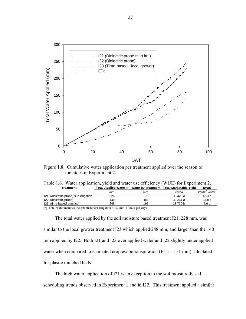
Figure 1.8. Cumulative water application per treatment applied over the season to
tomatoes in Experiment 2.
Table 1.6. Water application, yield and water use efficiency (WUE) for Experiment 2.
[z] Total water includes the establishment irrigation of 52 mm (1 hour per day)
The total water applied by the soil moisture based treatment I21, 228 mm, was
similar to the local grower treatment I23 which applied 248 mm, and larger than the 140
mm applied by I22. Both I21 and I23 over applied water and I22 slightly under applied
water when compared to estimated crop evapotranspiration (ETc = 151 mm) calculated
for plastic mulched beds.
The high water application of I21 is an exception to the soil moisture-based
scheduling trends observed in Experiment 1 and in I22. This treatment applied a similar
Treatment Total Applied Water [z] Water by Treatment Total Marketable Yield IWUEmm mm kg/ha kg/m 3 water
I21 (dielectric probe) sub-irrigation 228 176 30 428 a 13.3 aI22 (dielectric probe) 140 88 33 261 a 23.8 bI23 (time-based practice) 248 196 18 730 b 7.6 a

28
amount of water (10% less) as the time based treatment I23, and was attributed to the
position of the soil moisture probe with respect to the irrigation line. The drip line for
this treatment was buried at a depth of 15 cm under the surface. The probe was however
positioned the same as I22 so that it averaged the soil moisture from the surface down to
a depth of 20 cm. The top 15 cm of soil would have remained dry due to little or no
capillary rise of water in the sandy soil. The probe’s position in the drier soil near the
surface resulted in few irrigation events being bypassed and savings were low (only
10%). A future recommendation for this setup of a buried irrigation line would be either
to reduce the soil moisture threshold, or a more recommended practice would be to bury
the soil moisture probe closer to the irrigation line and active root zone. Further study
needs to address the implications of moving the probe within the interconnected wetting
zone of a buried line, and the effective rooting zone.
Significant differences in yield were recorded, and both soil moisture-based
treatments I21 and I22 had higher marketable yields, 30,428 and 33,621 kg/ha
respectively, than I23 which yielded 18,730 kg/ha. The high water application of I21
(buried drip) compared to I22 resulted in the irrigation water use efficiency for I21 being
closer to the time-based treatment I23. Cumulative leaching data is summarized in Table
1.7, and the cumulative volume leached over the season and the cumulative load of
nitrate-nitrogen leached over the season are presented graphically in Figures 1.9 and 1.10
respectively.
29
DAT
0 20 40 60 80 100
Vol
ume
Leac
hed
(mm
)
0
10
20
30
40
50
60
Figure 1.9. Cumulative volume of leachate collected in the lysimeters per treatment over
the season for Experiment 2.
DAT
0 20 40 60 80 100
Load
NO
3-N
leac
hed
(kg/
ha)
0
10
20
30
40
50
Figure 1.10. Cumulative nitrate-nitrogen load leached per treatment over the season for
Experiment 2.

30
Table 1.7. Average volume leached and nitrate-nitrogen load leached per treatment for Experiment 2
Total Treatment Total Treatmentmm mm kg/ha kg/ha
I21 (Dielectric probe + subirri.) 20.6 14.5 a 5.8 3.7 aI22 (Dielectric probe) 6.8 5.0 b 6.7 6.2 aI23 (Time-based - local grower) 42.8 36.3 c 37.3 34.1 b
NO3-N loadTreatment
Volume leached
† Different letters depict statistically different means for P ≤ 0.05 (Tukey Kramer HSD method)
The leaching volume differed significantly for all three treatments. Treatment I21
had a higher leached volume (14.5 mm) than I22 (5.0 mm) during the treatment period,
corresponding to the higher water application, but both soil moisture based treatments
were considerably lower than the time-based treatment I23 (36.3 mm). Total season
leached volumes (including the establishment period) were on average 31% higher than
leaching volumes during the treatment period. The load of nitrogen load leached by the
soil moisture based treatments I1 and I2 were 3.7 and 6.2 kg/ha respectively and
translated into a 89 to 84 % reduction from I23 (34.1 kg/ha for the treatment period).
Although treatment I21 had high water applications and higher leached volumes than I22,
the loads of nitrate leached were lower, a result of the fertigation line at the surface being
above the buried irrigation line. The irrigation water did not pass through the soil zone
near the surface with highest nitrate concentration. Better correlation of the buried drip
irrigation tape and the soil moisture probe in this treatment would most likely further
reduce leaching due to lower water applications closer to that of I22. The increase in
load of nitrate-nitrogen being leached towards the end of the season in treatment I22 was
due to an increase in water applied towards the end of the season after a late increase in
plant biomass and higher crop water requirements. The increase in irrigation water
applied should not have substantially increased the leaching, as the crop according to soil

31
moisture status required the water applied. Better knowledge of position of the soil
moisture probe in the root zone may help further reduce the portion of this water that is
leached.
Comparison of results
A summary of the percentage changes in value of the dependant variables of the
soil moisture-based treatments from the time-based local grower treatment are presented
in Table 1.8. Averages for the soil moisture-based treatments are presented to help
highlight the trends when compared to traditional time based practices.
The soil moisture-based treatments applied less water than the time-based
schedules for both experiments. For the treatment period the soil moisture-based
schedule treatments of Experiment 1, I11 and I12 achieved 77% and 80% water savings
compared to the local grower treatment respectively, and the treatments I21 and I22 for
Experiment 2 yielded 10% and 64% water savings over the local grower treatment
respectively.
Table 1.8. Average values and the percentage change from the local grower treatment for the dependant variables measured in two experiments of tomatoes corresponding to different irrigation scheduling treatments.
Tensiometer ECH2O Average ECH2O+sub irri. ECH2O Average I11 I12 (I11+I12)/2 I21 I22 (I21+I22)/2
Dependent variable Gravelly loam Gravelly loam Gravelly loam sand sand sandTotal Irri. Water (mm) -70 -82 -8 -50Treatment Irri. Water (mm) -77 -90 -10 -64Yield (kg/ha) 10 -12 62 78IWUE (kg/m3) 275 400 75 216Total Vol. Leached (mm) -73 -75 -74 -52 -84 -68Treatment Vol. Leached (mm) -78 -91 -85 -60 -86 -73Total Load N-NH4 (kg/ha) -97 -97 -97 - - -Treatment Load N-NH4 (kg/ha) -88 -92 -90 - - -Total Load N-NO3 (kg/ha) -64 -46 -55 -84 -82 -83Treatment Load N-NO3 (kg/ha) -64 -94 -79 -89 -82 -85Total Load DP (kg/ha) -66 -76 -71 - - -Treatment Load DP (kg/ha) -70 -89 -79 - - -Total Load TP (kg/ha) -53 -77 -65 - - -Treatment Load TP (kg/ha) -56 -85 -70 - - -
Experiment 1 Experiment 2Soil moisture-based treatments Percentage change from the time based (local grower) treatment

32
A large portion of the water savings occurred in the early part of the season when
the crop was small and water requirements were low. The soil moisture based treatments
minimized water application to suit crop needs during this period, while the fixed time
based schedules over applied irrigation. This can be seen in Figures 1.4 and 1.7 showing
the cumulative plots of water for the season for each experiment. Total water savings for
the full season were similar but on average over both experiments 8% lower than the
treatment period. The water applied during establishment was 52 mm for both
experiments, which was a significant contribution towards the total application for the
soil moisture-based treatments. Irrigation rates decreased dramatically once the soil
moisture-based treatments began to operate, but this did not have an effect on plant
growth. This suggests that the amount of water applied during the establishment period
could be reduced. Further studies could determine what the practical level of
establishment irrigation is needed before irrigation is switched to soil moisture-based
scheduling, without affecting transplant growth and yield. Limiting water to the
transplants must be done so with caution, as the plants roots are small and not well
established. Probe placement at this period is critical.
The irrigation rates for the soil moisture-based treatments were below those of the
crop water requirements as calculated by historical evapotranspiration and crop
coefficients presented in Maynard et al. (2004). Amayreh and Abed (2005) conducted a
study on field grown tomatoes in the Jordan Valley to test the effects drip irrigation and
plastic mulch would have on evapotranspiration and crop coefficients. Their study
showed that crop coefficients using drip irrigation and plastic mulch were 36% lower
than the crop coefficients in FAO 56 which assume a uniformly planted field. These

33
results match those obtained by Brouwer and Heibloem (1986). This explains the lower
crop needs and subsequent water use of the soil moisture-based treatments compared to
traditional ETc calculations.
Yields from Dade County (Experiment 1) were above the Florida average of 39,295
kg/ha suggested by Maynard et al. (2004), and ranged from 40,000 to 49,000 kg/ha.
Total marketable yields from Experiment 1 were derived from two harvests for the crop.
The Citra County (Experiment 2) yields were lower than average ranging from 18,600 to
33,200 kg/ha. Total marketable yield comprised of two harvests. Poor canopy
development in the plants early stage as a result of disease and some nutrient stress, most
likely reduced yields to some extent. Furthermore, the wettest treatment I4 in the Citra
County (Experiment 2) had yields that were significantly lower than the two soil
moisture-based treatments I1 and I2. This may be a result of the increased nitrogen
leaching and a loss of nutrient from the root zone of the crop. Another potential yield
reducing factor was that during the middle of the season the plastic mulch started to loose
its physical integrity, and provide incomplete coverage on a few of the beds. Where this
occurred, the bed was recovered with plastic mulch manually. The damage was random,
and did not occur near any instrumentation, but its effect on the yields is not certain. The
mulch is designed to start to break down after a period of time, sufficiently longer than
the cropping season. Reasons for this mulch to weaken after only 7 weeks are not
known. The suppliers were contacted and informed of the problem.
Irrigation water use efficiencies (IWUE) were much higher for the soil moisture
based treatments. Soil moisture-based treatment IWUE’s were 275 and 400% higher for
Experiment 1 and 75 and 216% higher for Experiment 2 than the corresponding time-

34
based local grower treatments. A previous experiment in the Miami-Dade County using
similar soil moisture based scheduling methodology by Muñoz-Carpena et al., (2004)
found IWUE’s of between 11 and 40 kg/m3. The high IWUE recorded for Experiment 1
in Miami-Dade County was also 40 kg/m3. This suggests that the methodology has the
potential for consistently efficient water use.
All nutrients tested for leaching showed substantial reductions in total loads of over
55% for the soil moisture-based treatments over the time based treatments. For surface
based drip irrigation and fertigation the volume of water applied appeared to be the
driving force, and volumes of leachate and nutrient loads followed water application
trends. For the sub irrigation of treatment I21 in Experiment 2 the high water and
leaching volumes did not displace much of the nutrients from the soil as the irrigation
was applied below the fertilizer application. The total leachate volumes averaged 74 and
68% lower for the Experiment 1 and Experiment 2 respectively. The lower amounts of
water passing through the root zone did not result in high concentrations of nutrients in
the leachate, as reductions in nutrient loads were equal to or higher the corresponding
reductions in leachate volumes. The highest reductions in nutrient load were recorded for
ammonia-nitrogen (averaged 90% for the treatment period) on Experiment 1 followed by
nitrate-nitrogen (85% for the treatment period) on Experiment 2. The nitrate-nitrogen
leaching in Experiment 1 had variability problems within treatments that may have
masked the results to some degree. The variability was higher for all nutrients in
Experiment 1 and was due to the smaller lysimeter capture area used. The smaller
capture area were more vulnerable to imperfect placement of the lysimeters under the
crop in the beds, but also had a higher variability of number of plants and emitters that

35
they contained. For future experiments lysimeters with large as possible capture areas
should be used to reduce leaching variability within treatments. This will be of particular
importance when finer soils are tested that have higher lateral movement of soil moisture.
The water applied to Experiment 2 was not replicated for each treatment. The
replications were for yield analysis and to account for soil heterogeneities. It would be
recommended to operate each replicate of the treatments independently in future
experiments. Each replicate would have its own soil moisture probe and control valve,
and give a better indication of the variability associated with the methodology, and help
eliminate the possibility of having one probe in an unrepresentative position for the
whole treatment.
The nutrient leaching data showed trends that correlated with the water application
amounts. Treatments with high water applications yielded higher volumes of leachate
and higher loads of nutrients passing through the root zone into the lysimeters. The form
of nitrogen being applied differed between the two experiments, as Experiment 1 applied
nitrogen in the ammonia form and Experiment 2 applied calcium nitrate. Both nitrate and
ammonia loads of nitrogen were determined from the leachate in Experiment 1 as the
ammonia nitrogen in the lysimeters could stand for as long as three weeks before it was
abstracted, and could undergo nitrification during this period. Both experiments showed
a significant reduction in leaching of nitrate, which is a contaminant of many surface and
groundwater resources in Florida, the US and around the world. The ability of soil
moisture-based irrigation to reduce nitrate loading to local water resources on coarse soils
is high. Further studies need to be conducted to test the effect different soils have on the
methods ability to reduce nutrient loading.

36
Conclusion
This series of two experiments confirmed the potential of soil moisture based
scheduling to reduce water applications as apposed to traditional time based schedules
and applied water less frequently and in higher volumes. Soil moisture based treatments
applied between 50 and 82% less water than comparative time based schedules which are
typically used for irrigation scheduling. The results show that the reduction in the
amount of water applied can be achieved without significant reductions in yield. The
reduced water application of the soil moisture based treatments translates to a reduction
in both volume of leaching, and the load of nutrients leached. Total nitrate leaching was
reduced by 55% and 83% for the two experiments and total phosphorous leaching was
65% lower. Greater reductions in loads leached (between 70 and 97% for all nutrients)
during just the treatment period were obtained for the soil moisture-based schedules and
suggest that there is potential for further savings at the beginning of the season. Potential
scheduling during the establishment must recognize the practical limits of saving water
and nutrients when the plants roots are limited. The reductions in nutrient losses could
provide a grower with the means to reduce application amounts and thus costs, and more
importantly reduce the risk of surrounding water resources to nutrient contamination.
This is critical to the sustainability of agriculture in Florida and many other areas of the
world, where increasing population and public environmental awareness introduces a
fierce competition for water resources.
38
CHAPTER 3 FERTIGATION METHODS FOR SOIL MOISTURE-BASED IRRIGATION OF
VEGETABLE CROPS
Introduction
Commercial vegetable production requires optimal fertilizer and water-use
management for high yields and maximum profits. In most cases nitrogen is the limiting
element to crop growth, especially on coarse-textured soils such as sands and gravels that
have low organic matter (Scholberg et al., 2001). Efficient use of water and fertilizers are
also highly critical for the sustainability of agriculture in increasingly competitive local
and world markets, and in competition with urban environments for resources (Hebbar et
al., 2004). In Florida vegetables are produced on nearly 120,000 ha and fertilizer is
needed for profitable production of high-quality vegetables in the State (Hochmuth,
2000). The optimum management of fertilizer can promote sustainability in several
ways, and application of N and K in excess of crop requirements can have significant
adverse effects (Hartz and Hochmuth, 1996). Firstly, fertilization represents a significant
input cost, accounting for 8 to 10 % of total cost of production for some vegetables.
Secondly, nutrients such as N or K can be lost due to leaching in the sandy soils of
Florida under excess irrigation or heavy rainfall. Finally nutrient management is
important because it reduces the nutrients introduced to the environment that have a
negative impact on the quality of surface and groundwater.
There has been significant work conducted on rates of N and K applied to vegetable
crops, and tomatoes in particular, and with improved nutrient and irrigation management

39
the maximum recommended rates have decreased in recent years. Applied fertilizers
used in Florida tomato production averaged 350-225-605 kg/ha as surveyed by the
Florida Agriculture Statistics Service for 1994 (Fla. Agr. Stat. Ser., 1995). These actual
applied rates exceed IFAS current maximum recommendations of 175-150-225 kg/ha N –
P2O5 – K2O, found through experiment to meet tomato requirements for high yields based
on soils with low P and K concentrations (Hochmuth and Hanlon, 1995). Achieving the
correct rate of fertilizer application is an essential part of optimal fertilizer management.
This however needs to be coupled with good irrigation practices as the application of
fertilizer and water are interlinked. Poor irrigation management and efficiencies affects
nutrient management. The higher applications of fertilizer than current recommendations
partially balance the effect of inefficient irrigation practices.
Improved Irrigation Management
Modern methods of using soil moisture to schedule irrigation are yielding
significantly improved irrigation water use, and at times has increased yield (Muñoz-
Carpena et al., 2005). A system has been developed by the University of Florida that
utilizes soil moisture probes to schedule on an automated irrigation system (Dukes and
Muñoz-Carpena, 2005). Water savings on average of 60 – 70% and up to 80% compared
to traditional time-based irrigation have been obtained by multiple experiments on
vegetable crops (tomatoes, bell peppers and zucchinis) on coarse soils in Florida. The
system applies water in small amounts and at frequent intervals (several times per day).
The soil water is kept within an optimal range for plant growth rather than being allowed
to dry out and then be completely refilled by a single large irrigation event. The
improved soil water management in the root zone of the crop decreases the potential for
loss of nutrients by the leaching due to the lack of excess applied water. Other essential

40
components of optimal fertilizer management are the method of application and the
frequency of application.
Fertigation
Clark et al., (1991) found improved water and fertilizer management using
tensiometers and fertigation with micro irrigation of market tomatoes produced on sandy
soils can result in reduced water and fertilizer applications as compared with current
irrigation methods. This statement brings two points into focus. Firstly as already stated
irrigation and fertilizer management are intricately linked. Secondly that fertigation
using surface and subsurface drip has proved to be in many applications, more effective
at supplying the crop with nutrients as needed by the crop.
Benefits of Fertigation
Dry fertilizers applied under traditional methods are generally not utilized
efficiently by the crop. In fertigation with drip, nutrients are applied through the emitters
directly into the zone of maximum root activity and consequently fertilizer use efficiency
can be improved compared to conventional methods of fertilizer application. Raskar,
(2003) reported significant increases in yields of banana when soluble fertilizer was
applied through fertigation compared to straight fertilizer. Hebbar et al. (2004)
conducted field experiments during two summers and found that 100% water soluble
fertilizer applied through fertigation had significantly higher yields than soil applied
treatments. Yields were similar for half-soil and half-fertigated treatments. Fertigation
also resulted in less leaching of NO3-N and K to deeper layers of sandy loam soil.
Fertilizer Injection
It is important to design the drip irrigation system so that fertilizer injection can be
achieved in a reasonable amount of time, and the crop is not over watered while

41
delivering the fertilizer. Concentrated materials are easier to inject because of the shorter
injection cycle required, for the same amount of nutrient. Growers should purchase as
high an analysis of liquid fertilizer as possible to avoid applying large amounts of water
(Hochmuth and Smajstrla, 1998). Research on a sand soil in Florida shows that 45
minutes (young tomato crop) to 1.5 hours (mature crop) would be sufficient to apply the
amount of water required by the crop during any one irrigation cycle (Smajstrla, 1985;
Clark et al., 1990). Fertigation and subsequent irrigation cycles longer than 1.5 hours on
a mature crop runs the risk of leaching the nutrients below the root zone. Leaching
occurs after a shorter duration on the gravelly loam soils in South Florida.
Fertilizers may be injected as a precisely managed level of concentration, or as a
bulk mass of fertilizer with possible varying concentration levels. Concentration
injection requires a precise injection system, and is more costly and complex than bulk
injection that simply involves the injection of a desired amount or volume of fertilizer
into the system. The injection system must be calibrated for the irrigation system it is to
be used within, or else expected applications will differ from actual applications.
Variations in operating pressure, system flow and even temperature can influence the
calibration of the system (Hotchmuth and Smajstrla, 1998).
Fertilizer application schedules
The current preplant fertilizer recommendations are a fraction of the total seasonal
fertilizer requirement, either liquid or dry, applied in the bed as a starter fertilizer for drip
irrigated crops (Hochmuth and Smajstrla, 1998). This starter fertilizer would contain all
the phosphorous (P) and micronutrients, and up to 40% of the N and K. In most cropping
situations approximately 35-45 kg/ha of N and K would suffice (Hochmuth and
Smajstrla, 1998). Maynard et al. (2003) suggested broadcasting all P2O5, micronutrients,
42
and 20-25% of the N and K2O in the bed area, for mulched drip irrigated crops. Preplant
application of P is common for at least two reasons. Soluble P sources are more
expensive than granular forms, and the potential problem of chemical precipitation in the
drip line is avoided.
Some research has found that applying some or all the fertilizer preplant provides
higher yields than just incremental applications through the season. This is most often
the case on soils with a higher percentage fine particles or more organic matter. Preplant
application of N (and K, if needed) is particularly important where initial soil levels are
low (Locasio et al., 1985), or where early-season irrigation requirements are low.
Preplanting fertilizer formulas of 6-6-12, 6-3-12 or 10-10-10 are satisfactory (Li et al.,
2002).
Locascio et al., (1997) applied N-K in three different proportions of preplant,
namely 0%, 40%, and 100% to tomato crops growing on an Arredondo fine sand and
only N as above to an Orangeburg fine sandy loam testing high in K. It was found that
the lowest yields on the fine sand occurred for the 100% preplant, intermediate yields for
the 0% preplant (all drip applied), and the highest yields for the 40% preplant and 60%
fertigation. On the sandy loam the highest yields were obtained from 100% preplant,
intermediate with 40% preplant and 60% drip applied, and lowest with all N drip applied.
This suggests that soil texture plays a major role in determining what methods of
fertilization are most appropriate.
A further component of the work conducted by Locascio et al., (1997) was to split
the drip applied fertilizer into 6 or 12 equal or variable applications through the season.
The variable application rate had most of the nutrients applied between weeks 5 and 10

43
after transplanting. For the 100% drip applied N on the sandy soil, yield was higher for
the 12 equal applications than the12 variable applications of N. While work continues to
optimize rates of N, P and K for different soils, the frequency of fertilizer application and
its effects on nutrient use efficiency remains less well understood. Thompson et al.,
(2003) stated that optimum fertigation intervals for drip-irrigated crops has not been well
researched. A study conducted subsequently by Thompson et al., (2003), found that
broccoli grown on a sandy loam soil did not respond to any increase in frequency of
fertigation using subsurface drip smaller than 28 days.
Frequent injection might be needed on sandy soils that do not retain large amounts
of nutrients, and for growers that wish to minimize injection pump size and cost (Hartz
and Hochmuth, 1996). Fertigation frequency however in most situations is not as
important as achieving a correct rate of nutrient application to the crops during a specific
period (Cook and Saunders, 1991). What must be kept in mind is that water management
and fertilizer management are linked. Changes in one program will affect the efficiency
of the other program.
Fertigation coupled with soil moisture-based irrigation
Automation of fertigation within a soil moisture-based irrigation system has the
potential for decreased labor as well as increasing water and nutrient savings. Fertilizer
can be injected with precise injection pumps on an independent automated schedule, or
the fertilizer can be continuously injected using a venturi injector. A drawback of the
automated injection pumping system is its cost. Venturi injectors are low cost devices
that have proven to provide adequately accurate injection rates for fertigation purposes.
Continuous injection with a venturi means injecting fertilizer each time an irrigation
event occurs. The flow of irrigation water across the venturi contraction causes a

44
pressure differential that sucks a liquid fertilizer solution into the distribution system
(Figure 2.1). Placing the venturi across a pressure-regulating device such as a valve, or
pressure regulator, or pump can enhance the pressure differential. Appendix A1 to A4
has different recommended layouts for increasing the pressure differential across a
venturi.
Figure 2.1. A venturi injector schematic showing flow directions and operating principle (adapted from Mazzei Injectors Inc.)
The venturi injection rate is relatively insensitive to flow rate, and is controlled
primarily by pressure at the inlet and outlet. Manufacturers such as Mazzei Injector
Corporation provide charts for their different models to calculate injection rates.
The concentration of fertilizer to be injected is determined by knowing the desired
fertilizer application rate, the injection rate of the venturi, and the injection time (in this
case the same as the irrigation schedule). For fixed time-based irrigation schedules the
irrigation schedule is predetermined and thus the injection time is known. For dynamic
soil moisture-based irrigation the duration of irrigation changes according to factors that
effect soil moisture level. The irrigation schedule will vary from season to season when
using soil moisture as the basis for scheduling. An estimate was needed to predict the
water use for the crop over the season. The crop evapotranspiration ETc is the IFAS
recommended method for determining water use. Previous experiments on tomatoes by
45
Munoz-Carpena et al. (2004) and (2005) reported consistent savings for two consecutive
experiments in the Miami-Dade County on tomatoes with the QIC and dielectric probe
soil moisture-based scheduling over the ETc schedule. The savings were 51% and 58%
for two experiments conducted during the winter seasons on Krome soil. By using
results of water savings by soil moisture based irrigation scheduling over ETc scheduling,
derived from experiments conducted by the University of Florida, expected water
applications can be derived. From these water applications, fertilizer solution
concentrations can be determined for a known injection delivery rate.
The aim of this research was to 1.) To test the management possibilities of
continuous fertigation coupled with soil moisture irrigation scheduling, 2.) Compare the
continuous ferigation with fixed event fertigation in terms of seasonal application rates,
labor and management requirements, and crop yield, and 3.) Make recommendations for
future research.
Methods and Materials
Fieldwork was conducted for two years to test the continuous fertigation method.
Both experiments were conducted on tomato crops, the first over the 2004/2005 winter
cropping season in South Florida on a calcareous gravelly soil and the second during the
2005 spring season in Central North Florida on a sandy soil. For each experiment fixed
event fertigation applied through drip lines was compared to continuous fertigation
integrated into a soil moisture-based irrigation schedule also applied through drip.
Tomatoes of the variety ‘FL 47’ were cropped on raised beds with plastic much spaced at
1.83 m. Sorghum-Sudan grass was grown as a cover crop the season prior to tomato
cropping for each experiment.

46
Experiment 1: South Florida gravelly soil
This first experiment was conducted during the winter season in South Florida at
the Tropical Research and Education Center, in Miami-Dade County on a gravel soil.
The field was divided into two regions, an Experiment Plot, and a Demostration Plot for
different purposes. The Experiment plot had different irrigation water scheduling
treatments and was used to determine the effects of scheduling methods on water use,
yield and leaching. Fertigation was conducted through a separate distribution system to
the irrigation water, and fertilizer was applied equally to all treatments on a fixed time-
based schedule. The Demonstration Plot tested continuous fertigation coupled with soil
moisture based irrigation, and provided visitors to the field with a display of a system
working as it would in practice. Fertilizer was applied as fertigation through the same
distribution system as the irrigation water. All injected into the same line that supplied
the irrigation water. All injection of the fertilizer for fertigation of this experiment was
carried out using venturi injectors (model no. 484, Mazzei Injector Crop., Bakersfield,
CA). The venturi injectors were installed across 10 m pressure regulators to help develop
adequate pressure differential (Figure 2.2 and 2.3). A downstream pressure of 10 meters
was chosen to minimize the pressure in the lay flat and thus reduce leaks but maintain
sufficient pressure for the drip tapes that were rated at 7 m operating pressure. The
upstream pressure to the venturi was the pressure inside the well tank of 25 m. The 484
model of Mazzei venturi injectors have an ideal documented injection rate of 64 L/hr
when with an upstream pressure of 25 m and a downstream pressure of 10m. This can be
seen in the tables (Mazzei Injector Inc.
http://www.mazzei.net/agriculture/tables/Performance%20Table%20Metric.pdf) in
Appendix A4.
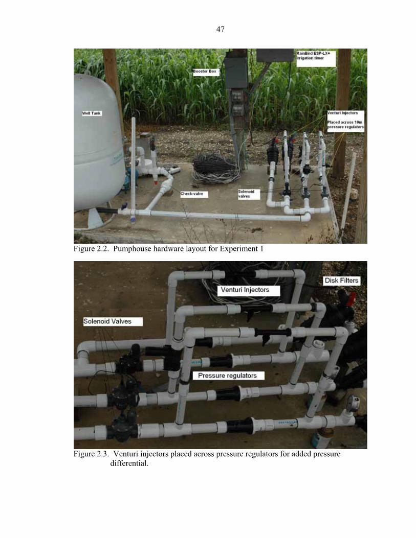
47
Figure 2.2. Pumphouse hardware layout for Experiment 1
Figure 2.3. Venturi injectors placed across pressure regulators for added pressure differential.
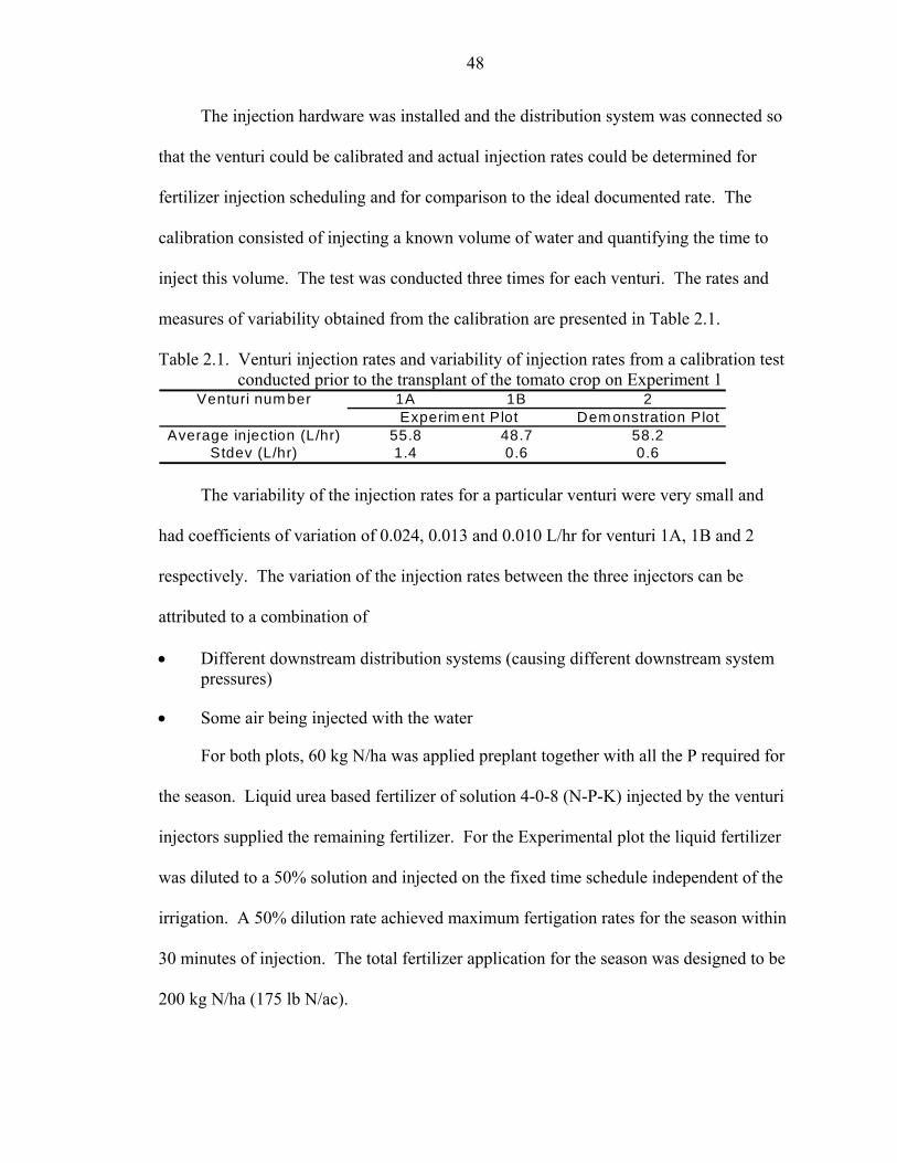
48
The injection hardware was installed and the distribution system was connected so
that the venturi could be calibrated and actual injection rates could be determined for
fertilizer injection scheduling and for comparison to the ideal documented rate. The
calibration consisted of injecting a known volume of water and quantifying the time to
inject this volume. The test was conducted three times for each venturi. The rates and
measures of variability obtained from the calibration are presented in Table 2.1.
Table 2.1. Venturi injection rates and variability of injection rates from a calibration test conducted prior to the transplant of the tomato crop on Experiment 1
The variability of the injection rates for a particular venturi were very small and
had coefficients of variation of 0.024, 0.013 and 0.010 L/hr for venturi 1A, 1B and 2
respectively. The variation of the injection rates between the three injectors can be
attributed to a combination of
• Different downstream distribution systems (causing different downstream system pressures)
• Some air being injected with the water
For both plots, 60 kg N/ha was applied preplant together with all the P required for
the season. Liquid urea based fertilizer of solution 4-0-8 (N-P-K) injected by the venturi
injectors supplied the remaining fertilizer. For the Experimental plot the liquid fertilizer
was diluted to a 50% solution and injected on the fixed time schedule independent of the
irrigation. A 50% dilution rate achieved maximum fertigation rates for the season within
30 minutes of injection. The total fertilizer application for the season was designed to be
200 kg N/ha (175 lb N/ac).
Venturi num ber 1A 1B 2Dem onstration Plot
Average injection (L/hr) 55.8 48.7 58.2Stdev (L/hr) 1.4 0.6 0.6
Experim ent Plot
49
For the Demonstartion plot’s continuous fertigation method integrated within the
soil moisture based irrigation scheduling, the irrigation schedule had to be predicted. It
was estimated from previous experiments conducted by Munoz-Carpena et al. (2004) and
(2005) that the water application for the soil moisture-based scheduling would be 40% of
theoretical crop evapotraspiration (which overestimates actual crop water needs for
plastic mulched beds). This estimate of water application (40% of theoretical ETc) was
divided over the season according to the crop curve. The total design fertilizer
application for this plot was 266 kg/ha (237 lb/ac). The required dilution of 4-0-8 liquid
fertilizer was initially 15% for the first 11 weeks of the season and then 11% for the last 2
to 3 weeks when fertilizer rates are reduced.
The actual fertilizer rate applied to the crop by the venturi’s on the time-based
schedule for the Experiment Plot, was 196 kg/ha (174 lbs/ac) which complied very well
with the IFAS recommended 175 lbs/ac. The continuous fertigation method in
Demonstration plot applied 285 kg N/ha (250 lbs N/ac) that was comparable to the
desired rate of 266 kg N/ha (237 lbs N/ac) by the procedure just mentioned (Figure X).
Yields for continuous fertigation coupled with soil moisture-based scheduling were
similar to yields achieved by treatment emulating local growers, and averaged 47 260
kg/ha (42 100 lbs/ac) and 45 110 kg/ha (40 180 lbs/ac) respectively.
A second experiment was conducted the following spring to further test the
continuous fertigation method on a different soil and season, and using a different
fertilizer.
Experiment 2: North Central Florida sandy soil
Tomatoes were grown on a fine sand soil using plastic mulched beds in North
Central Florida at the Plant Research and Education Unit in Citra County. For this
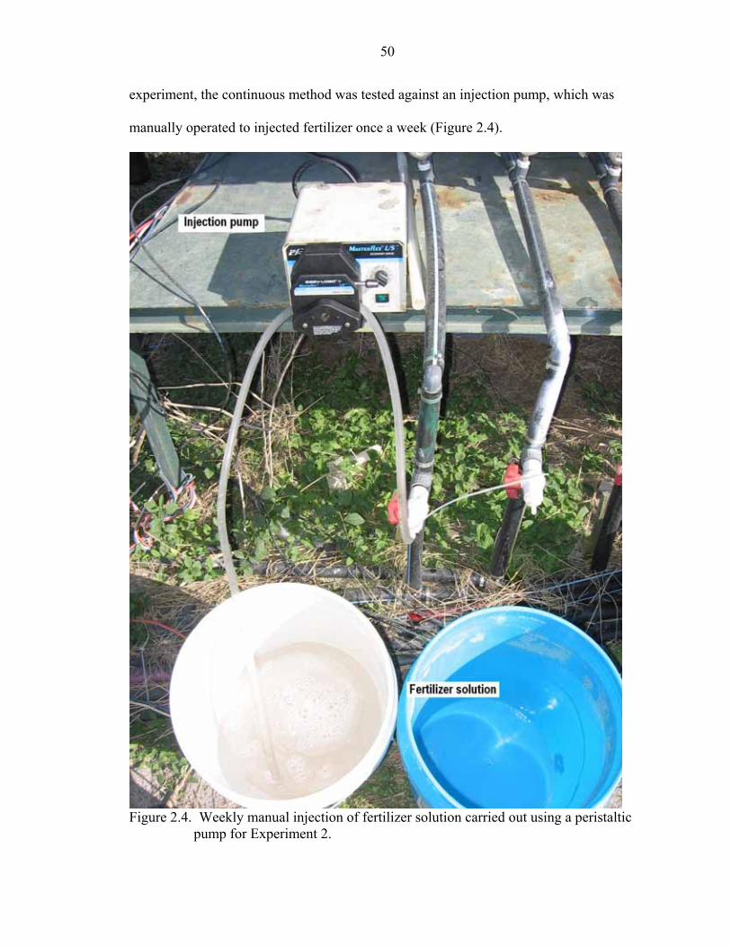
50
experiment, the continuous method was tested against an injection pump, which was
manually operated to injected fertilizer once a week (Figure 2.4).
Figure 2.4. Weekly manual injection of fertilizer solution carried out using a peristaltic pump for Experiment 2.
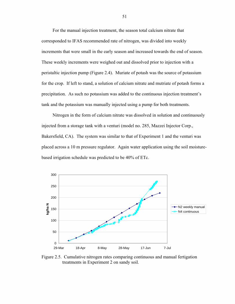
51
For the manual injection treatment, the season total calcium nitrate that
corresponded to IFAS recommended rate of nitrogen, was divided into weekly
increments that were small in the early season and increased towards the end of season.
These weekly increments were weighed out and dissolved prior to injection with a
peristaltic injection pump (Figure 2.4). Muriate of potash was the source of potassium
for the crop. If left to stand, a solution of calcium nitrate and mutriate of potash forms a
precipitation. As such no potassium was added to the continuous injection treatment’s
tank and the potassium was manually injected using a pump for both treatments.
Nitrogen in the form of calcium nitrate was dissolved in solution and continuously
injected from a storage tank with a venturi (model no. 285, Mazzei Injector Corp.,
Bakersfield, CA). The system was similar to that of Experiment 1 and the venturi was
placed across a 10 m pressure regulator. Again water application using the soil moisture-
based irrigation schedule was predicted to be 40% of ETc.
Figure 2.5. Cumulative nitrogen rates comparing continuous and manual fertigation treatments in Experiment 2 on sandy soil.
0
50
100
150
200
250
300
29-Mar 18-Apr 8-May 28-May 17-Jun 7-Jul
kg/h
a N
N2 weekly manualN4 continuous

52
The plot of fertilizer applied through the season (Figure 2.5) shows how although a
constant concentration of fertilizer was injected for the continuous fertigation treatment,
the rate of application varied considerably through the season. Nutrient application rate
was below the desired rate for most of the season. Lower than average temperatures
during this period reduced evapotransoiration and corresponding irrigation amounts
based on soil moisture. Because irrigation drives the fertilizer injection the fertigation
was also low. The increase in application rate later in the season (from 7th June onwards)
can be attributed to an increase in irrigation as a result of increased evapotranspiration.
The increase in evapotranspiration was the result of increasing biomass and plant cover,
and a period of warmer weather conditions in early summer.
The continuous fertigation system integrated within soil moisture-based irrigation
is very successful at providing a system that is low cost with low labor and management
requirements during average years and conditions. Due to the coupled nature of the
water and nutrient applications the system is however vulnerable to weather and any
other conditions that cause deviations from expected irrigation application. The lower
irrigation water application itself is not the problem, as the crop may have needed less
water due to cooler conditions. The soils moisture–based scheduling applies water as
needed by the crop. The potential harm is the lower fertilizer application induced by
lower irrigation amounts. The crop may have required less water but not less nutrients.
Combining continuous methods with scheduled fertigation
A solution to the problems of fertigation within a soil moisture-based irrigation
system is to combine the best components of the two methods of continuous fertigation
and fixed schedule manual injection. The benefit of the continuous fertigation is the low
cost of the venturi injector and the ease of management and low labor requirements. By

53
decoupling the fertigation from the irrigation scheduling based on soil moisture, the
systems vulnerability to extreme weather and conditions is mitigated.
Soil moisture-based irrigation as practiced by the University of Florida uses an
irrigation timer to schedule potential events. These prescheduled events trigger a soil
moisture probe to be queried. If soil moisture is below a set threshold a solenoid valve is
opened and the event initiated. If the soil moisture is above a set threshold, then the
event is bypassed and water saved. For vegetable crops the maximum daily water
requirements are divided into 4 or 5 sub-events. To implement continuous fertigation
with a venturi on a fixed schedule, one of the sub-events is dedicated to fertigation
independent of soil moisture status. Any of the sub-events within the day could be used
for fertigation as they are all sufficiently short to avoid excessive leaching and nutrient
loss. Herdel et al. (2001) state that the uptake of nutrients and nitrate in particular is
dependent on plant-internal relations and not nutrient availability, but is three times
higher during the day than at night. The first event of the day is the most appropriate as
subsequent irrigation events may be bypassed if the water for fertigation wet the soil
sufficiently. If the fertigation event were later in the day, the soil may already be wet
from prior events, but water will still be added by fertigation, increasing the potential for
leaching. Furthermore, the first event of the day is the most likely due to drying out of
the soil (although at a somewhat lower rate than the day), and the best time for a fixed
event.
The recommended control and distribution system hardware for fixed continuous
fertigation within a soil moisture-based irrigation schedule is presented in Figure 2.6.
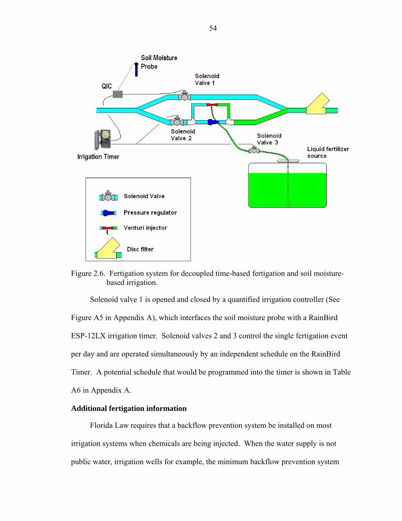
54
Figure 2.6. Fertigation system for decoupled time-based fertigation and soil moisture-based irrigation.
Solenoid valve 1 is opened and closed by a quantified irrigation controller (See
Figure A5 in Appendix A), which interfaces the soil moisture probe with a RainBird
ESP-12LX irrigation timer. Solenoid valves 2 and 3 control the single fertigation event
per day and are operated simultaneously by an independent schedule on the RainBird
Timer. A potential schedule that would be programmed into the timer is shown in Table
A6 in Appendix A.
Additional fertigation information
Florida Law requires that a backflow prevention system be installed on most
irrigation systems when chemicals are being injected. When the water supply is not
public water, irrigation wells for example, the minimum backflow prevention system

55
requires a check valve, low pressure drain, and vacuum breaker on level piping between
the point of injection and the irrigation pump to prevent water and chemicals flowing
back to the water source (Smajstrla et al., 1985). No backflow prevention is required if
the water source is not public water, and no chemicals are injected into the irrigation
system (Smajstrla et al., 1994). To extend the life of the system, and to maintain high
irrigation uniformity by keeping the emitters unblocked, a filter should be placed after the
fertilizer injection. A 200-mesh size disc filter should be used.
Fertilizer should be purchased that is soluble and quickly available to the plant.
Some liquid fertilizers are slow release and although my be effective at reducing leaching
for single large applications are not suitable for daily injection when the nutrients are
applied as the crop needs them. Suitable formulations are 4-0-8 (N-P-K) liquid fertilizer,
and soluble potassium nitrate (KNO3). Suggested IFAS daily fertigation rates are
presented in Table 2.2.
Table 2.2. IFAS suggested daily fertigation rates for tomatoes.
† When 25% total N and K is applied preplant, the first two weeks can be omitted.
To adjust the fertilizer application to follow crop growth and needs it is easier to
adjust the fertigation time on the controller than it is to change the solution of a large
volume of fertilizer in the tank. The concentration should be set so that the longest
fertigation event is similar to the length of the sub-daily events. To ensure that the
venturi is working correctly and that nutrients are reaching the crop, a simple check is to
Week aftertransplant N (lbs/ac) N (kg/ha) K (lbs/ac) K (kg/ha)1 and 2 1.5 1.7 1.5 1.73 and 4 2 2.2 2 2.2
5 through 11 2.5 2.8 3 3.412 2 2.2 2 2.213 1.5 1.7 1.5 1.7
Season total 200 225 225 253
Daily Injection rateNitrogen Potassium

56
record and check the level of the fertilizer solution in the tank. The level can be
compared to design levels that can be easily calculated from the injection schedule and
venturi injection rate.
Conclusions
Soil moisture-based irrigation has high potential for water savings and accurate soil
moisture management for optimal crop growth. Fertigation combined with soil moisture-
based irrigation can reduce leaching of nutrients and delivers nutrients to the root zone of
the crop. Continuous fertigation is a viable low cost and labor method that is driven by
irrigation water application. When coupled with soil moisture-based irrigation
scheduling it requires a prediction of season irrigation amount to determine
concentrations to be applied for the upcoming season, and is vulnerable to weather, crop
and soil effects that may reduce evapotrasnpiration and thus irrigation amount.
Decoupling the continuous fertigation from soil moisture-based scheduling gives the
system the reliability of a time-based schedule, while maintaining the benefits of both soil
moisture-based irrigation and low cost and labor fertigation. The two operations remain
connected as the water that is applied with the fertilizer during fertigation contributes
towards the soil moisture and irrigation is scheduled accordingly.

57
CHAPTER 4 DIELECTRIC CAPACITANCE SOIL MOISTURE PROBE CALIBRATION AND
SPATIAL SOIL MOISTURE DYNAMICS STUDY
Introduction
Optimal management of irrigation requires systematic estimation of soil moisture
status to determine both the volume and timing of irrigation. Soil water content must be
maintained between specific lower and upper levels so that water is not limiting to plant
growth, but leaching is prevented (Morgan et al. 2001). Measurements of soil moisture
status under irrigated crops over time is part of integrated management that aims to
minimize the economically detrimental effects of both under and over-irrigation on crop
yield and quality, the environmental costs of wasted water and energy, and impaired
water quality due to leaching. Integrated irrigation management to achieve optimal soil
moisture levels may be accomplished by utilizing soil moisture monitoring devices in
conjunction with rainfall records and knowledge of plant needs (Munoz-Carpena et al.
2002).
When using drip irrigation to apply water to the crop, the volume and profile of soil
wetted by a single emitter is important. This must be known in order to determine the
total number of emitters required to wet a large enough volume of soil to ensure that the
plants water requirements are met. The volume of soil wetted from a point source is
primarily a function of the soil texture and structure, application rates and the total
amount of water applied (Lubana and Narda, 1998). Sandy soils also have low amounts
of total soil water, and narrow ranges of plant-available soil water. Morgan et al. (2001)

58
found that the range of 100-50% plant available soil water in Apopka sand, a fine sand
found in Florida, was only 0.08-0.045cm3cm-3 soil water content by volume and –5 to –
15 kPa soil water tension.
The wetting profile in the root zone is dynamic and affected by crop root
interactions with the soil. As the crop biomass increases, evapotranspiration will increase
and use more of the volume of water in the wetted profile. Crop and system factors that
can affect the dynamic wetting profile and soil water volume other than soil hydraulic
properties and emitter delivery rate are crop growth stage, root length and structure, and
mulch type when mulches are used. The volume and shape of wetting profiles is not only
important for emitter spacing and system design, but is important for soil moisture-based
scheduling using soil moisture sensors. According to Lubana and Narda (1998) very
little attention has been paid to the estimation of soil water distribution during drip
irrigation under realistic field conditions.
Due to the very vertical movement of water in coarse soils such as sand, large soil
moisture gradients can exist across a small horizontal distance. Sensors placed in two
positions only 15 cm apart within the wetting zone of an emitter can have very different
readings during and after an irrigation event. Sands are often water repellant and
according to Bauters et al. (1998) research has shown that water repellant soils and sands
have unstable wetting fronts and finger-like wetting patterns. These wetting patterns are
generally directly related to the soil moisture retention curve (SWRC). It has also be
shown (Kutilek and Nielsen, 1994) that laboratory determined SWRC’s are significantly
shifted to larger soil moisture values for given soil matric potentials compared to those
obtained under field conditions. The differences between laboratory and in-situ SWRCs

59
are generally thought to be a result of a combination of entrapped air and/or alteration of
bulk density in the laboratory samples.
Because sensors provide the data that drives the automatic control of soil moisture
based irrigation they are an extremely important component, and understanding the
operating principles of a sensor and the effects of soil type on its performance is
imperative (Zazueta et al., 1994). Poor sensor position that does not represent
demographic soil moisture conditions in the root zone can either result in crop water
stress, or over irrigation that negates the water saving capabilities of soil moisture
scheduling. From field experiments conducted on two tomato crops, it became
increasingly apparent how important knowledge of the effects of sensor placement
position within the plastic mulched bed was for precise and reliable soil moisture
management on coarse soils.
The University of Florida has tested different types of sensors on plastic mulched
vegetable crops. Munoz-Carpena et al., (2005) found that switching tensiometers worked
well but required consistent refilling and maintenance, and granular matrix sensors
behaved erratically due to slow response times. A dielectric capacitance probe (ECH2O,
Decagon Devices Inc., Pullman, WA) has proven to work reliably with low maintenance
and is considerably lower cost than TDR sensors. A general calibration curve is available
for the ECH2O probe for sandy loam soils and accuracies of up to 1% soil moisture
content by volume can be achieved using the general calibration curve for most soils.
This equation for this linear curve is presented in Equation 4.1.
Soil moisture = 0.0007*mV – 0.29 [4.1]

60
Campbell (2005a) has advised that a soil-specific calibration be conducted on soils
with high sand or salt content. Campbell (2005b) has also noted a linear response of
sensor out put to temperature, although recommends that temperature effects in soils are
small due to the mediating effect of soil on temperature fluxes. Campbell (2005c) found
that the ECH2O probe was generally not affected by low salinity on most soils, but
readings of soil moisture deviated significantly from actual values on sandy soils with
high salinity.
Considering the lack of knowledge of soil moisture profiles within the dynamic
emitter-root zone continuum, the low plant available water content of sandy soils, and the
importance of good data from a soil moisture probe for soil moisture-based irrigation
scheduling, an experiment was conducted on the sandy soils at the plant science research
and education unit (PSREU). The aims of this experiment were to:
1. Calibrate the ECH2O soil moisture probe for the fine sand soils found at the Plant science research and education unit.
2. Derive an in-field soil moisture characteristic curve for the fine sand
3. Gain knowledge of the spatial variability of soil moisture within the root zone of a plastic mulched crop and its corresponding effects of probe placement position on irrigation scheduling
4. Determine the effects of factors that may influence the dielectric capacitance probes mV readings
Methods and Materials
An irrigation field trial on a zucchini crop was conducted during the fall season at
the Plant Science Research and Education Unit in Citra County, Central North Florida.
The irrigation experiment was conducted to test the effects of soil moisture-based
scheduling compared to regular time based scheduling on water and nutrient use for
plastic mulched vegetables. The soil moisture-based treatments employed dielectric
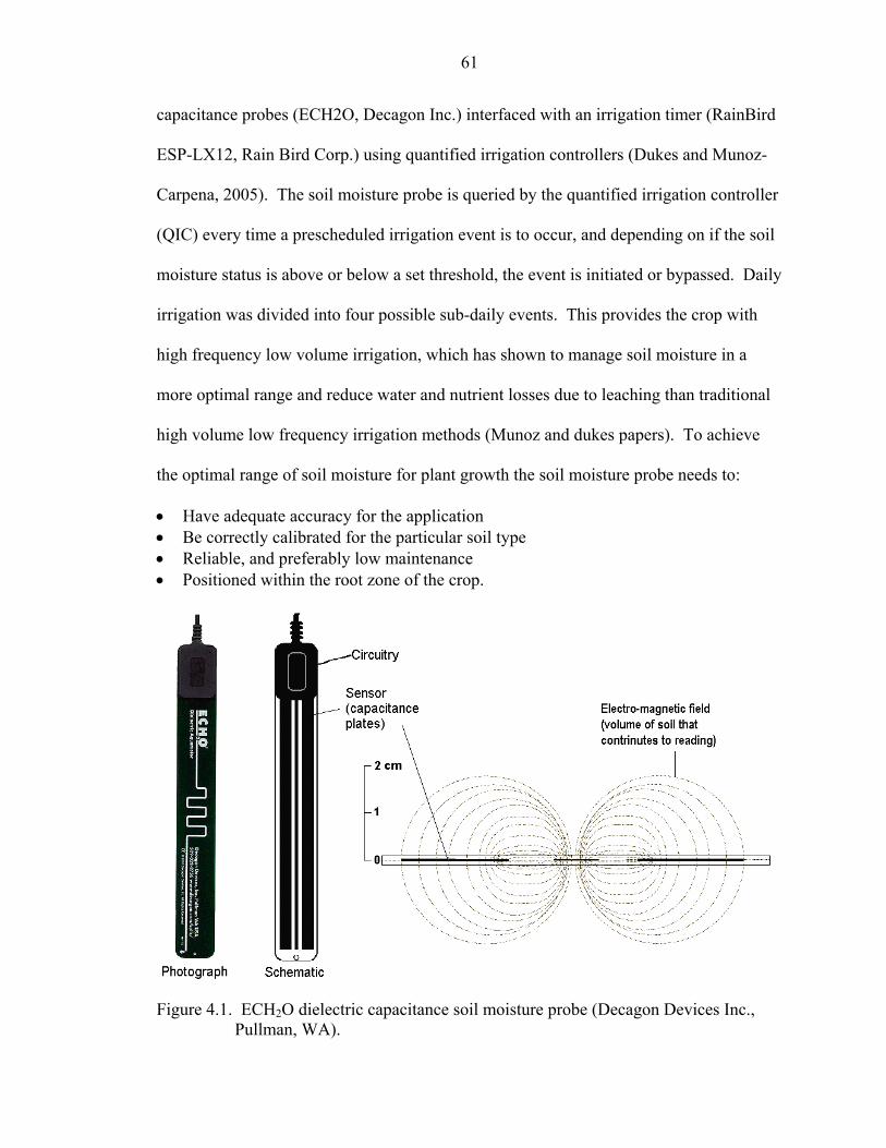
61
capacitance probes (ECH2O, Decagon Inc.) interfaced with an irrigation timer (RainBird
ESP-LX12, Rain Bird Corp.) using quantified irrigation controllers (Dukes and Munoz-
Carpena, 2005). The soil moisture probe is queried by the quantified irrigation controller
(QIC) every time a prescheduled irrigation event is to occur, and depending on if the soil
moisture status is above or below a set threshold, the event is initiated or bypassed. Daily
irrigation was divided into four possible sub-daily events. This provides the crop with
high frequency low volume irrigation, which has shown to manage soil moisture in a
more optimal range and reduce water and nutrient losses due to leaching than traditional
high volume low frequency irrigation methods (Munoz and dukes papers). To achieve
the optimal range of soil moisture for plant growth the soil moisture probe needs to:
• Have adequate accuracy for the application • Be correctly calibrated for the particular soil type • Reliable, and preferably low maintenance • Positioned within the root zone of the crop.
Figure 4.1. ECH2O dielectric capacitance soil moisture probe (Decagon Devices Inc.,
Pullman, WA).

62
The dielectric probe being used for the experiment has an accuracy of typically ±
0.03 m/m or (3% volumetric moisture content) and a resolution of 0.002 m3/m3 (0.1%).
With soil-specific calibration accuracies of ± 0.01 m/m are possible Campbell (2005).
The probe dimensions (Model EC-20 in Figure 4.1) are 25.4cm × 3.17cm × 0.15cm. The
probe determines the soil moisture from measures of the bulk conductivity of the soil in a
region of soil approximately 2 times the width of the probe (4cm) and averages the
reading across the length of the shaft (Figure 4.1). The manufacturers provide
calibrations for basic soil types, but a soil-specific calibration of the probe was conducted
to improve the accuracy of the soil moisture data being used to schedule irrigation and
monitor soil moisture for research purposes. The calibration was conducted in the field,
as laboratory studies often do not correlate with real conditions in the field. The in field
calibration would also allow a comparison between the soil moisture probes being used to
collect data and the probes scheduling the irrigation. A check could be made to test
whether the threshold for irrigation scheduling corresponded to appropriate soil moisture
levels.
To determine the spatial variability of soil moisture in the area that probe
placement has conventionally been used by the University of Florida, square grids of nine
dielectric capacitance (ECH2O) probes spaced 14 cm apart were replicated in three beds
of various irrigation scheduling treatments. The grids were centered directly between
two plants, which were planted about 10 cm away of the drip line (Figure 4.2). This was
the same position used for the single dielectric capacitance probe that was scheduling
water to the crop.
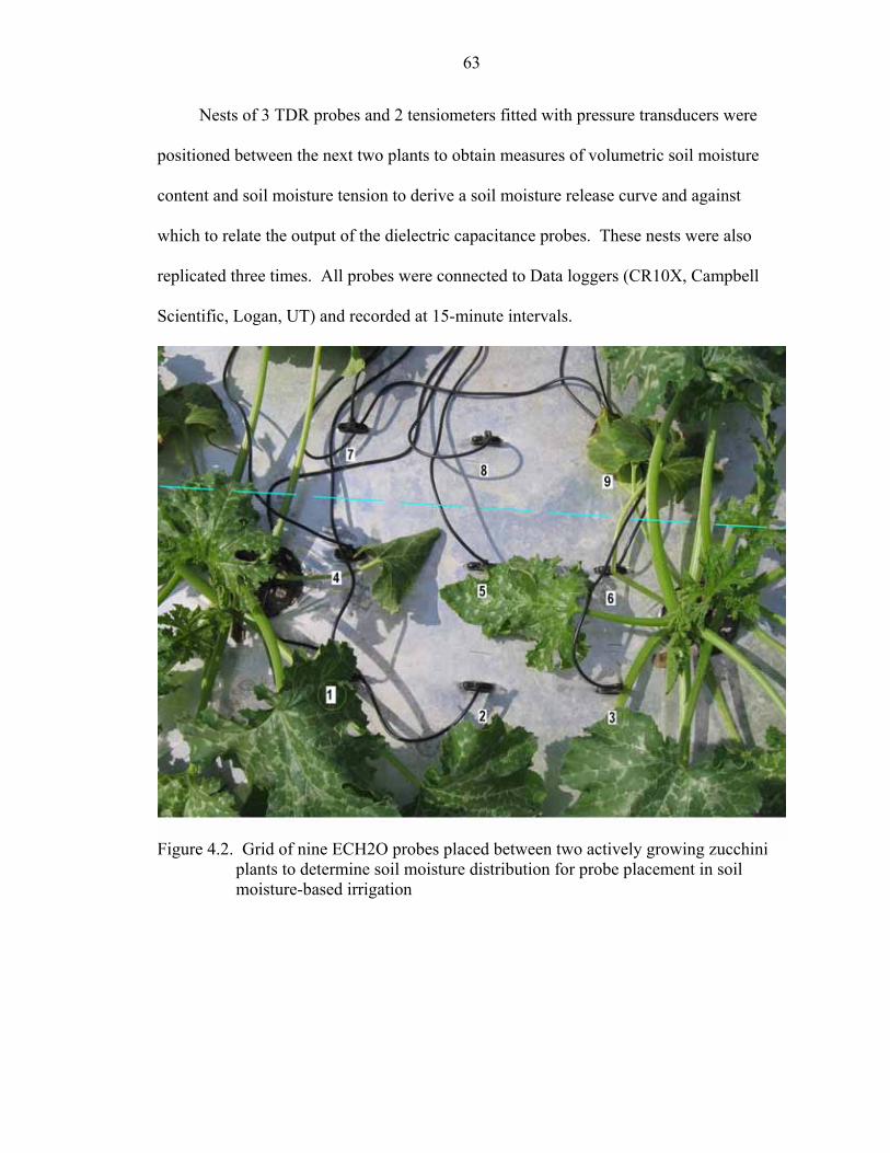
63
Nests of 3 TDR probes and 2 tensiometers fitted with pressure transducers were
positioned between the next two plants to obtain measures of volumetric soil moisture
content and soil moisture tension to derive a soil moisture release curve and against
which to relate the output of the dielectric capacitance probes. These nests were also
replicated three times. All probes were connected to Data loggers (CR10X, Campbell
Scientific, Logan, UT) and recorded at 15-minute intervals.
Figure 4.2. Grid of nine ECH2O probes placed between two actively growing zucchini plants to determine soil moisture distribution for probe placement in soil moisture-based irrigation

64
Figure 4.3. TDR nest to measure soil moisture for corresponding to mV irrigation threshold set point.
Once a sufficient period of data was obtained to determine the spatial distribution
of soil moisture using the grid of 9 dielectric capacitance probe grids, the probe
configurations were changed to calibrate the dielectric capacitance probes mV output
against the TDR soil moisture readings. Because the instruments were initially placed
between two different plants with potentially different drip emitter positions, direct
relations between soil moisture and mV readings were giving highly variable results. The
dielectric capacitance probes were moved next to the TDR probes, as close as possible
without interference. Two dielectric capacitance probes were placed next to each TDR
centered between two plants and replicated twice for treatments I1 and I2. The
replications were to help determine the inherent variability that exists due to different

65
plants, emitter positions and possibly even soil moisture characteristics of the soil along
the length of bed. A mean soil moisture vs dielectric capacitance probe mV curve could
then be derived which may better describe the probe soil relationship.
The irrigation system that was providing the crop with water was designed to
maintain soil moisture within as close to optimal soil moisture conditions as possible.
While this was good for the crop, it was not possible to derive extreme points for the soil
moisture release curve, namely the very dry and very wet regions of the curve. To obtain
these points, instruments were installed at the end of a bed, and once sufficient irrigation
had been provided to establish the plants containing the instruments, the irrigation was
terminated. Three tensiometers and three dielectric capacitance probes were installed
between two plants (Figure 4.4). The plants in this portion of the bed continued to
transpire and the soil moisture dropped towards wilting point. The probe cables were not
long enough to reach the ends of the beds from the CR10X data loggers. According to
the dielectric capacitance (ECH2O) user manual posted by Decagon Devices Inc. (Anon,
2005), any data logger that can produce a 2.5 to 5V excitation with approximately 10-
millisecond duration and read a volt-level signal with 12-bit or better resolution should be
compatible with the ECHO probes. The current requirement at 2.5V is around 2mA, and
at 5V it is 7-8mA. As such a small Hobo data logger (HOBO event logger, Onset
Computer Corp. Inc., Bourne, MA), was used to power and record the ECH2O probes
output. The small data loggers have the capacity to simultaneously record four separate
readings. It was found however that the first port had insufficient excitation period to
power up the ECH2O probes and that good data was obtained for the other three probes.
This method of data capture can provide a small low cost alternative to standard data

66
loggers, especially for a few remote probes. The only maintenance needed was replacing
the batteries. The batteries life was determined by the logging interval. Logging every
15 minutes, the batteries only needed to be changed once during the season (13 weeks)
when three probes were operating. To ensure correct operation of the logger, it was
placed in a watertight container (zip-lock bag) and covered with aluminum foil to prevent
overheating.
Figure 4.4. Nest of dielectric capacitance probes and tensiometers used to generate the drier points of the soil moisture release curve for the fine sand at PSREU.
The probe nests and positions used gave a good indication of the soil moisture
status in the center of the bed between plants. To better understand the soil moisture
distribution in a plants entire root zone an intensive probe layout was installed towards
then end of the crop season once the roots had reached maturity in spatial distribution. A

67
grid containing 33 dielectric capacitance probes was installed in one of the beds, and the
fertilizer was terminated to this bed to avoid any salinity effects on the soil moisture
readings. The grid covered the whole width of the bed, and was spread between three
plants, completely covering the root zone of the middle plant (Figure 4.5).
Figure 4.5. Probe grid of 33 dielectric capacitance probes to determine spatial dynamics in the root zone of a mature zucchini crop in plastic mulched bed
The data from the probes was analyzed and plotted in Sigmaplot Version 9
software. The software was used to generate 2 and 3D images to obtain visual
representations of the spatial distributions. A first order Loess spatial smoothing function
was applied to the data to generate a smooth 3-D image due to the distances between
point readings.
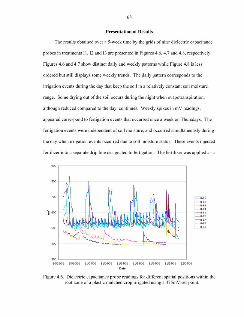
68
Presentation of Results
The results obtained over a 5-week time by the grids of nine dielectric capacitance
probes in treatments I1, I2 and I3 are presented in Figures 4.6, 4.7 and 4.8, respectively.
Figures 4.6 and 4.7 show distinct daily and weekly patterns while Figure 4.8 is less
ordered but still displays some weekly trends. The daily pattern corresponds to the
irrigation events during the day that keep the soil in a relatively constant soil moisture
range. Some drying out of the soil occurs during the night when evapotranspiration,
although reduced compared to the day, continues. Weekly spikes in mV readings,
appeared correspond to fertigation events that occurred once a week on Thursdays. The
fertigation events were independent of soil moisture, and occurred simultaneously during
the day when irrigation events occurred due to soil moisture status. These events injected
fertilizer into a separate drip line designated to fertigation. The fertilizer was applied as a
300
400
500
600
700
800
900
10/25/05 10/30/05 11/04/05 11/09/05 11/14/05 11/19/05 11/24/05 11/29/05 12/04/05
Date
mV
I1-E1I1-E2I1-E3I1-E4I1-E5I1-E6I1-E7I1-E8I1-E9
Figure 4.6. Dielectric capacitance probe readings for different spatial positions within the
root zone of a plastic mulched crop irrigated using a 475mV set-point.
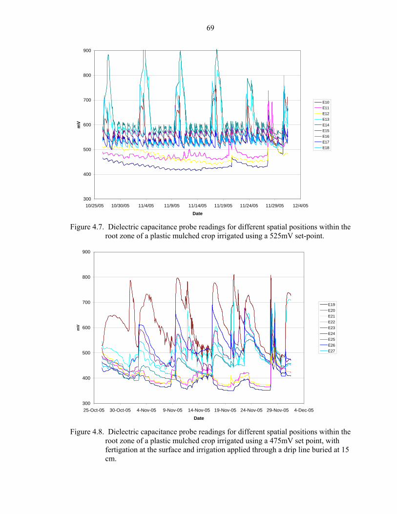
69
300
400
500
600
700
800
900
10/25/05 10/30/05 11/4/05 11/9/05 11/14/05 11/19/05 11/24/05 11/29/05 12/4/05
Date
mV
E10E11E12E13E14E15E16E17E18
Figure 4.7. Dielectric capacitance probe readings for different spatial positions within the
root zone of a plastic mulched crop irrigated using a 525mV set-point.
300
400
500
600
700
800
900
25-Oct-05 30-Oct-05 4-Nov-05 9-Nov-05 14-Nov-05 19-Nov-05 24-Nov-05 29-Nov-05 4-Dec-05
Date
mV
E19E20E21E22E23E24E25E26E27
Figure 4.8. Dielectric capacitance probe readings for different spatial positions within the
root zone of a plastic mulched crop irrigated using a 475mV set point, with fertigation at the surface and irrigation applied through a drip line buried at 15 cm.
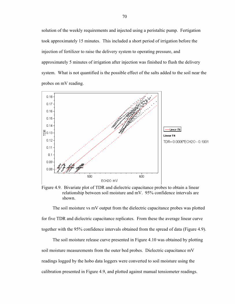
70
solution of the weekly requirements and injected using a peristaltic pump. Fertigation
took approximately 15 minutes. This included a short period of irrigation before the
injection of fertilizer to raise the delivery system to operating pressure, and
approximately 5 minutes of irrigation after injection was finished to flush the delivery
system. What is not quantified is the possible effect of the salts added to the soil near the
probes on mV reading.
Figure 4.9. Bivariate plot of TDR and dielectric capacitance probes to obtain a linear
relationship between soil moisture and mV. 95% confidence intervals are shown.
The soil moisture vs mV output from the dielectric capacitance probes was plotted
for five TDR and dielectric capacitance replicates. From these the average linear curve
together with the 95% confidence intervals obtained from the spread of data (Figure 4.9).
The soil moisture release curve presented in Figure 4.10 was obtained by plotting
soil moisture measurements from the outer bed probes. Dielectric capacitance mV
readings logged by the hobo data loggers were converted to soil moisture using the
calibration presented in Figure 4.9, and plotted against manual tensiometer readings.
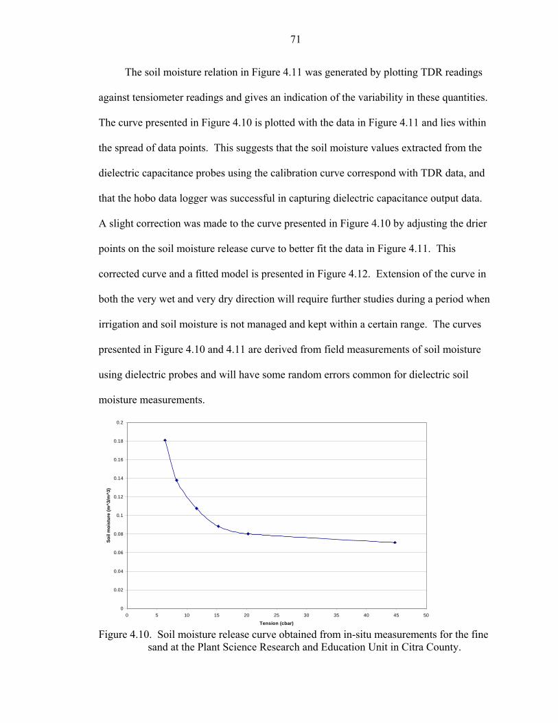
71
The soil moisture relation in Figure 4.11 was generated by plotting TDR readings
against tensiometer readings and gives an indication of the variability in these quantities.
The curve presented in Figure 4.10 is plotted with the data in Figure 4.11 and lies within
the spread of data points. This suggests that the soil moisture values extracted from the
dielectric capacitance probes using the calibration curve correspond with TDR data, and
that the hobo data logger was successful in capturing dielectric capacitance output data.
A slight correction was made to the curve presented in Figure 4.10 by adjusting the drier
points on the soil moisture release curve to better fit the data in Figure 4.11. This
corrected curve and a fitted model is presented in Figure 4.12. Extension of the curve in
both the very wet and very dry direction will require further studies during a period when
irrigation and soil moisture is not managed and kept within a certain range. The curves
presented in Figure 4.10 and 4.11 are derived from field measurements of soil moisture
using dielectric probes and will have some random errors common for dielectric soil
moisture measurements.
0
0.02
0.04
0.06
0.08
0.1
0.12
0.14
0.16
0.18
0.2
0 5 10 15 20 25 30 35 40 45 50
Tension (cbar)
Soil
moi
stur
e (m
^3/m
^3)
Figure 4.10. Soil moisture release curve obtained from in-situ measurements for the fine
sand at the Plant Science Research and Education Unit in Citra County.
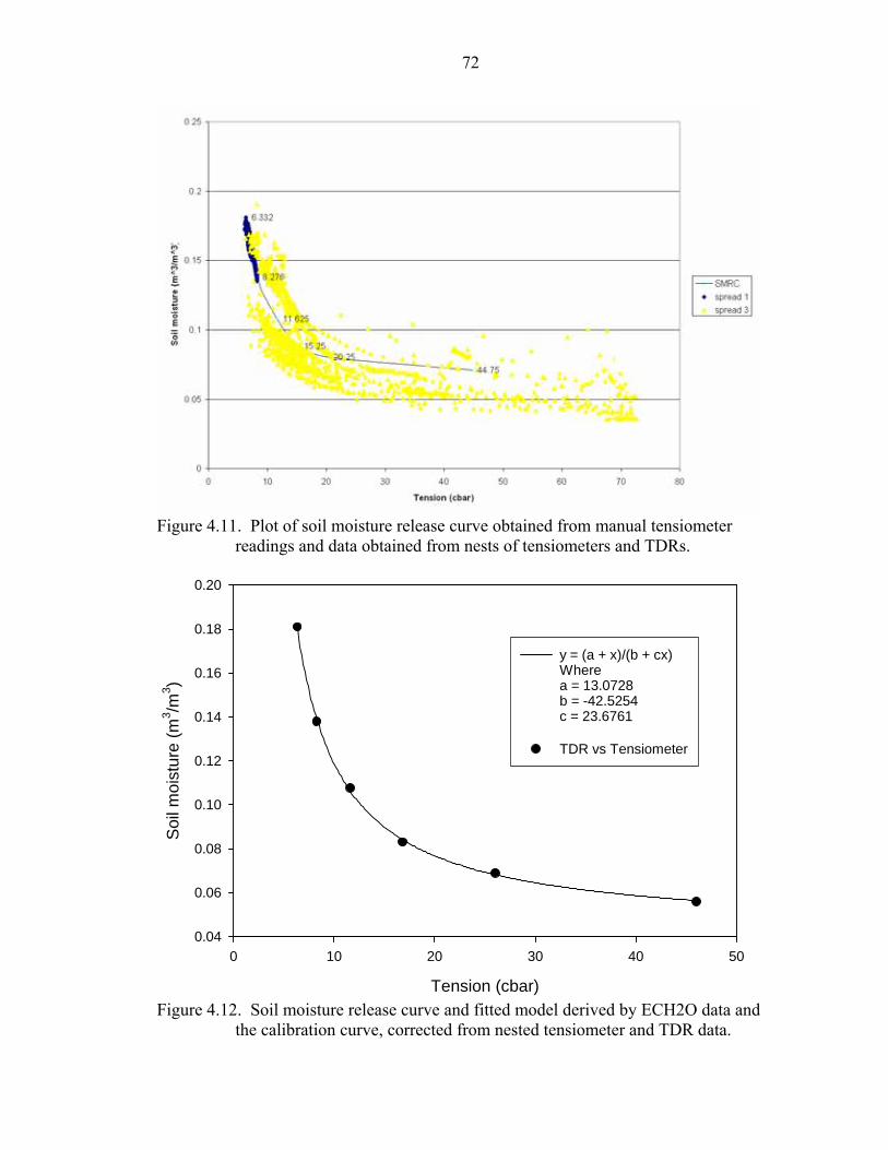
72
Figure 4.11. Plot of soil moisture release curve obtained from manual tensiometer
readings and data obtained from nests of tensiometers and TDRs.
Tension (cbar)
0 10 20 30 40 50
Soi
l moi
stur
e (m
3 /m3 )
0.04
0.06
0.08
0.10
0.12
0.14
0.16
0.18
0.20
y = (a + x)/(b + cx)Wherea = 13.0728b = -42.5254c = 23.6761
TDR vs Tensiometer
Figure 4.12. Soil moisture release curve and fitted model derived by ECH2O data and
the calibration curve, corrected from nested tensiometer and TDR data.
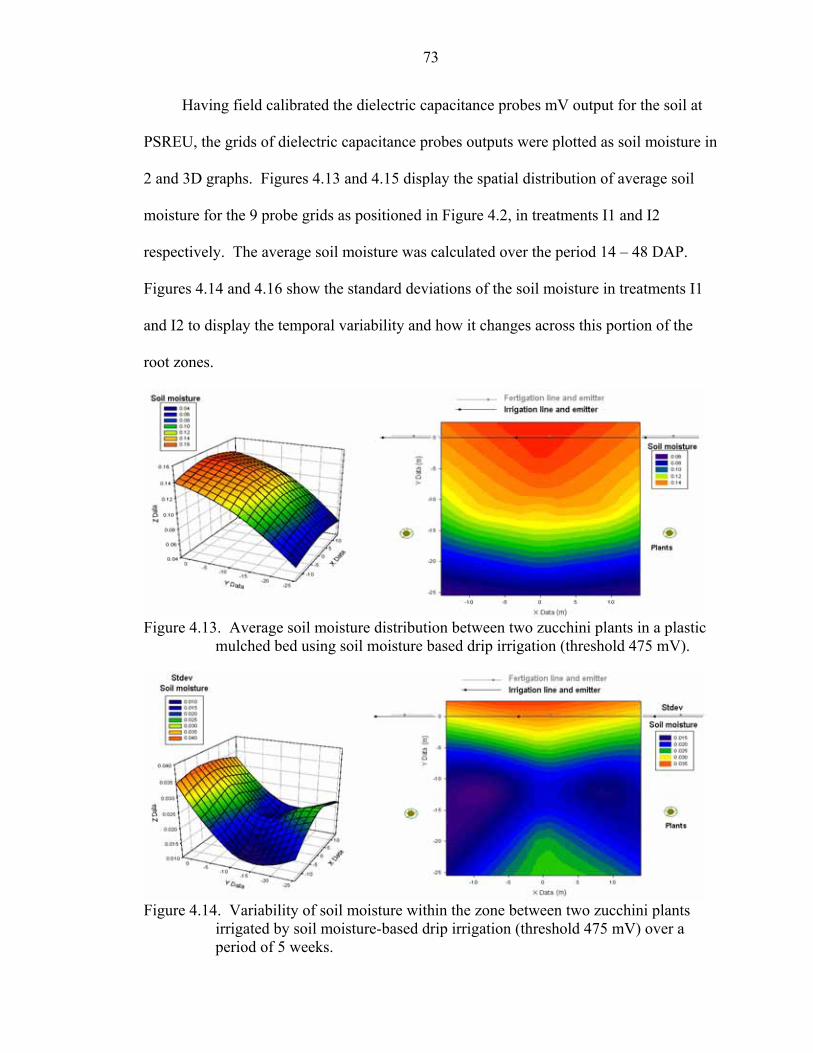
73
Having field calibrated the dielectric capacitance probes mV output for the soil at
PSREU, the grids of dielectric capacitance probes outputs were plotted as soil moisture in
2 and 3D graphs. Figures 4.13 and 4.15 display the spatial distribution of average soil
moisture for the 9 probe grids as positioned in Figure 4.2, in treatments I1 and I2
respectively. The average soil moisture was calculated over the period 14 – 48 DAP.
Figures 4.14 and 4.16 show the standard deviations of the soil moisture in treatments I1
and I2 to display the temporal variability and how it changes across this portion of the
root zones.
Figure 4.13. Average soil moisture distribution between two zucchini plants in a plastic
mulched bed using soil moisture based drip irrigation (threshold 475 mV).
Figure 4.14. Variability of soil moisture within the zone between two zucchini plants
irrigated by soil moisture-based drip irrigation (threshold 475 mV) over a period of 5 weeks.
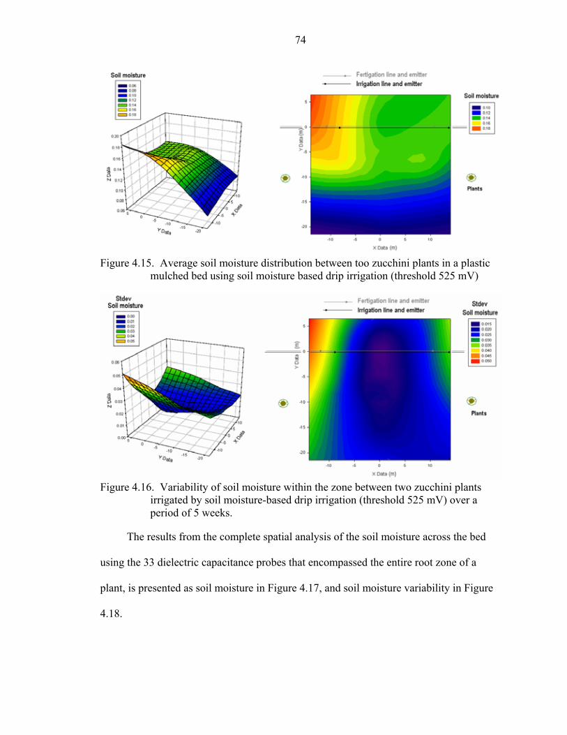
74
Figure 4.15. Average soil moisture distribution between too zucchini plants in a plastic
mulched bed using soil moisture based drip irrigation (threshold 525 mV)
Figure 4.16. Variability of soil moisture within the zone between two zucchini plants
irrigated by soil moisture-based drip irrigation (threshold 525 mV) over a period of 5 weeks.
The results from the complete spatial analysis of the soil moisture across the bed
using the 33 dielectric capacitance probes that encompassed the entire root zone of a
plant, is presented as soil moisture in Figure 4.17, and soil moisture variability in Figure
4.18.
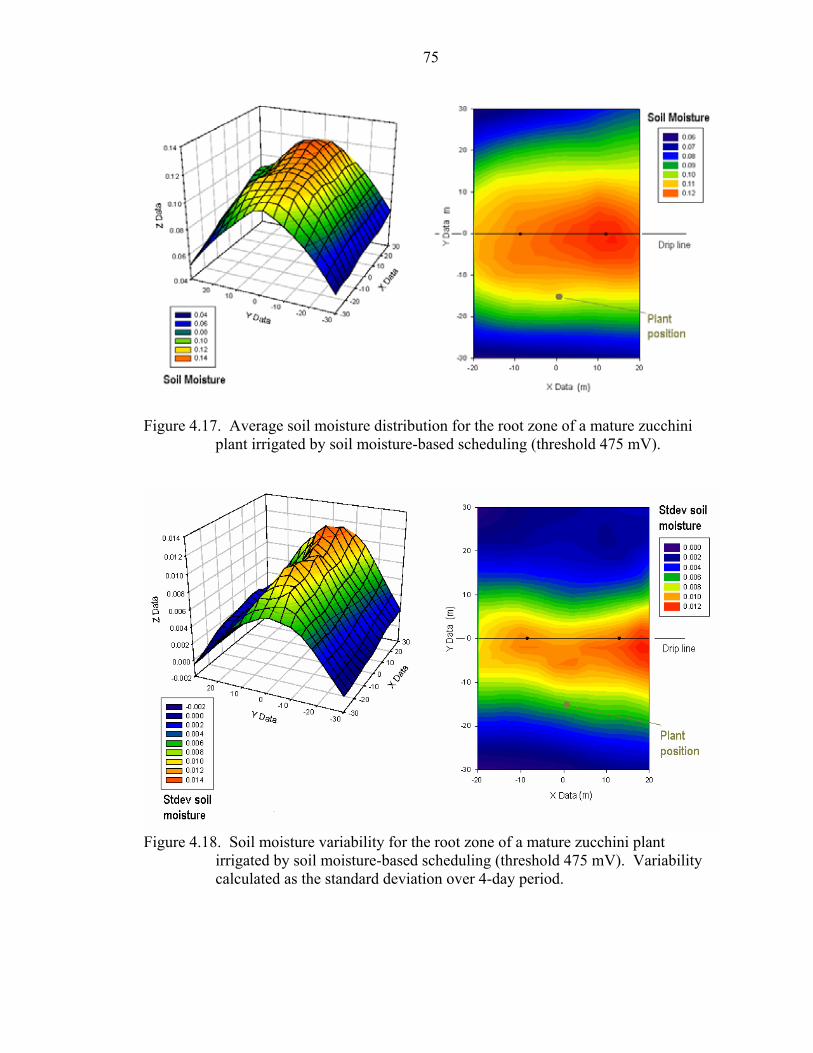
75
Figure 4.17. Average soil moisture distribution for the root zone of a mature zucchini
plant irrigated by soil moisture-based scheduling (threshold 475 mV).
Figure 4.18. Soil moisture variability for the root zone of a mature zucchini plant
irrigated by soil moisture-based scheduling (threshold 475 mV). Variability calculated as the standard deviation over 4-day period.
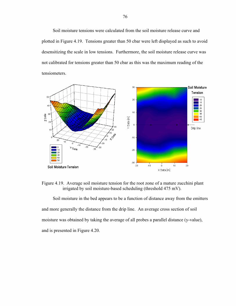
76
Soil moisture tensions were calculated from the soil moisture release curve and
plotted in Figure 4.19. Tensions greater than 50 cbar were left displayed as such to avoid
desensitizing the scale in low tensions. Furthermore, the soil moisture release curve was
not calibrated for tensions greater than 50 cbar as this was the maximum reading of the
tensiometers.
Figure 4.19. Average soil moisture tension for the root zone of a mature zucchini plant
irrigated by soil moisture-based scheduling (threshold 475 mV).
Soil moisture in the bed appears to be a function of distance away from the emitters
and more generally the distance from the drip line. An average cross section of soil
moisture was obtained by taking the average of all probes a parallel distance (y-value),
and is presented in Figure 4.20.
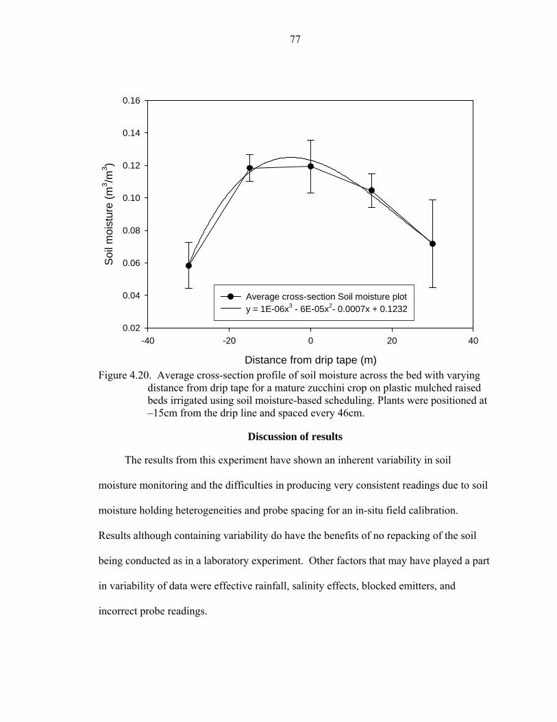
77
Distance from drip tape (m)
-40 -20 0 20 40
Soi
l moi
stur
e (m
3 /m3 )
0.02
0.04
0.06
0.08
0.10
0.12
0.14
0.16
Average cross-section Soil moisture ploty = 1E-06x3 - 6E-05x2- 0.0007x + 0.1232
Figure 4.20. Average cross-section profile of soil moisture across the bed with varying
distance from drip tape for a mature zucchini crop on plastic mulched raised beds irrigated using soil moisture-based scheduling. Plants were positioned at –15cm from the drip line and spaced every 46cm.
Discussion of results
The results from this experiment have shown an inherent variability in soil
moisture monitoring and the difficulties in producing very consistent readings due to soil
moisture holding heterogeneities and probe spacing for an in-situ field calibration.
Results although containing variability do have the benefits of no repacking of the soil
being conducted as in a laboratory experiment. Other factors that may have played a part
in variability of data were effective rainfall, salinity effects, blocked emitters, and
incorrect probe readings.

78
Rainfall
Rainfall did have an effect on some dielectric capacitance probe readings, and soil
moisture spikes were noted during rainfall event periods. This was evident in Figure
4.21, where some probes experienced spikes in soil moisture during rainfall periods and
others did not. The probes that had a higher incidence of effective rainfall were those
near the periphery of the bed, away from the cover of the plant biomass. This was
however not a clear trend.
Figure 4.21. Soil moisture time series showing how soil moisture spikes during rainfall events are limited to probes on exterior of bed that are not significantly influenced by irrigation
The cause of rainfall affecting some probes and not others may have been cover for
some probes from the plant canopy, or random ponding on the plastic mulch. Figure 4.21
shows how the outer probes (E1, E2 and E3) all spike during rainfall events, but not
during normal irrigation events. The effect of rainfall on soil moisture readings is limited
0
0.05
0.1
0.15
0.2
0.25
0.3
11/19/2005 11/21/2005 11/23/2005 11/25/2005 11/27/2005 11/29/2005
Date
Soil
moi
stur
e
I2 E1I2 E2I2 E3I2 E4I2 E5I2 E6I2 E7I2 E8I2 E9
50
40
30
20
10
0
Rainfall (mm)
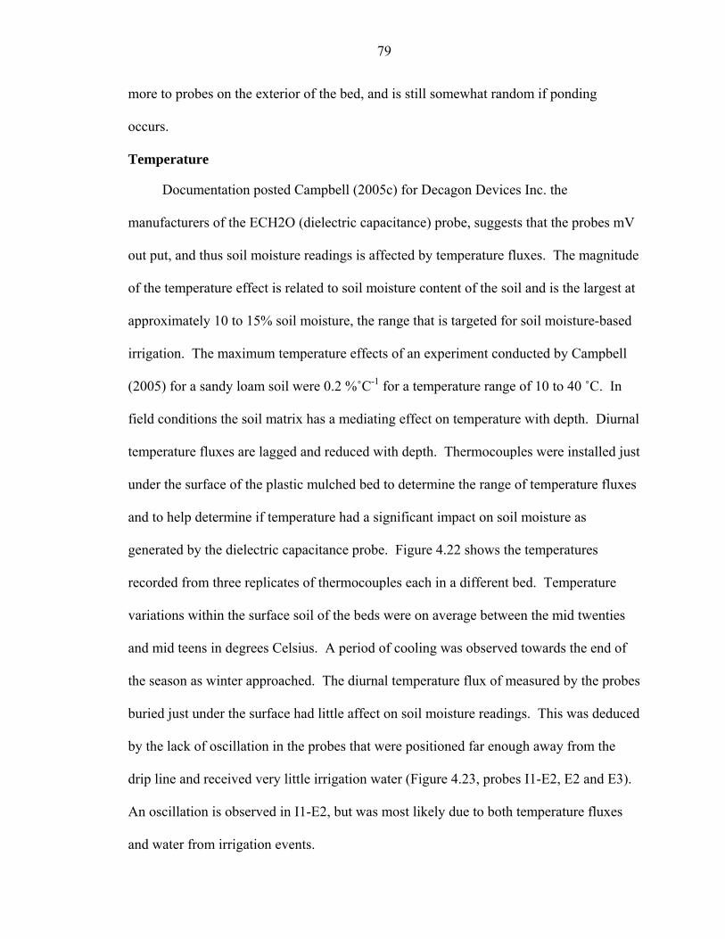
79
more to probes on the exterior of the bed, and is still somewhat random if ponding
occurs.
Temperature
Documentation posted Campbell (2005c) for Decagon Devices Inc. the
manufacturers of the ECH2O (dielectric capacitance) probe, suggests that the probes mV
out put, and thus soil moisture readings is affected by temperature fluxes. The magnitude
of the temperature effect is related to soil moisture content of the soil and is the largest at
approximately 10 to 15% soil moisture, the range that is targeted for soil moisture-based
irrigation. The maximum temperature effects of an experiment conducted by Campbell
(2005) for a sandy loam soil were 0.2 %˚C-1 for a temperature range of 10 to 40 ˚C. In
field conditions the soil matrix has a mediating effect on temperature with depth. Diurnal
temperature fluxes are lagged and reduced with depth. Thermocouples were installed just
under the surface of the plastic mulched bed to determine the range of temperature fluxes
and to help determine if temperature had a significant impact on soil moisture as
generated by the dielectric capacitance probe. Figure 4.22 shows the temperatures
recorded from three replicates of thermocouples each in a different bed. Temperature
variations within the surface soil of the beds were on average between the mid twenties
and mid teens in degrees Celsius. A period of cooling was observed towards the end of
the season as winter approached. The diurnal temperature flux of measured by the probes
buried just under the surface had little affect on soil moisture readings. This was deduced
by the lack of oscillation in the probes that were positioned far enough away from the
drip line and received very little irrigation water (Figure 4.23, probes I1-E2, E2 and E3).
An oscillation is observed in I1-E2, but was most likely due to both temperature fluxes
and water from irrigation events.

80
Figure 4.22. Temperature fluxes within three plastic mulched beds in the fall season of 2005. Thermocouples were buried approximately 15 mm beneath the surface.
The arrow in Figure 4.23 shows the increase in apparent soil moisture that could
have been from temperature changes as it warmed up in the morning. This increase in
soil moisture occurs before 9:00 am, the occurrence of an irrigation event. The other
probes show only a very small increase during the warm period in the day. The
maximum deviation from mean soil moisture for I1-E2 if only temperature changes were
considered, was only 0.35%.
Taking the potential for irrigation events to be contributing towards the increase,
actual temperature effects on soil moisture are most likely lower. From these results, and
the general spread of soil moisture readings using dielectric sensing within a soil
medium, the deduction is made that the probes buried vertically in the top 22 cm of soil
are not significantly affected by normal diurnal fluxes in temperature.
10
12
14
16
18
20
22
24
26
28
30
25-Oct-05 30-Oct-05 04-Nov-05 09-Nov-05 14-Nov-05 19-Nov-05 24-Nov-05 29-Nov-05 04-Dec-05
Date
Deg
rees
C Temp I1Temp I2Temp I3

81
0
0.05
0.1
0.15
0.2
0.25
0.3
11/12/05 11/12/05 11/13/05 11/13/05 11/14/05 11/14/05 11/15/05 11/15/05 11/16/05
Date
Soil
moi
stur
e
I1-E1I1-E2I1-E3I1-E4I1-E5I1-E6I1-E7I1-E8I1-E9
Irrigation events
Figure 4.23. Time series of soil moisture in bed I1 to show limited effects of temperature
on outer probes that receive little irrigation water.
Salinity
Figures 4.25,4.26 and 4.27 show that soil moistures determined by applying the
linear calibration to the ECH2O probe output have considerable spikes that correspond
with the days that fertigation occurred. These considerable spikes are not simulated in
the soil moisture data determined by TDR measures. Different factors that could have
caused these spikes in soil moisture as determined by the dielectric capacitance probes
were examined. Rainfall only had a limited effect in probes that were not covered by the
crop canopy, and the rainfall did not occur on a weekly cycle as the spikes in soil
moisture did. Temperature, a possible reason for deviation of dielectric capacitance
probe output showed to cause less than a 0,35% change in soil moisture. Furthermore
fluxes in temperatures were on a diurnal cycle, and not a weekly effect. The third and

82
possible external factor that may have caused spikes in soil moisture as read by the
dielectric capacitance probes was salinity effects. The spikes in mV were highest just
after feritigation events, when both water and fertilizer were introduced to the soil. From
the 20-minute duration of fertigation events, the system should have applied
approximately 0.67 mm of water to the soil. For the 20cm depth that the probes averages
the soil moisture over, this should result in only a 3.4% increase in soil moisture.
Corresponding increases in the soil moisture readings by TDR during the fertigation
events were only a few percent (Figures 4.25, 4.26 and 4.27). TDR data is assumed to be
sufficiently accurate to compare the dielectric capacitance data against, as TDR readings
are generally considered immune to salinity unless the salinity is so server that it masks
the peak-to-peak frequency in the signal. The dielectric capacitance probes close to the
fertigation line for treatments I1 and I2 showed increases of up to 15% in soil moisture
(Figures 4.25 and 4.26). Considering the negligible effects that all other likely factors
mentioned had on dielectric capacitance probes output, it is proposed that high salinity
after fertigation events is causing an increase in soil electrical conductivity, which is
possibly transferred into a higher bulk conductivity and thus mV readings measured by
the dielectric capacitance probes. A 12% higher reading in soil moisture by the dielectric
capacitance probes than the TDR readings would equate to an over reading of 170 mV by
the dielectric capacitance. Campbell (2005c) showed an increase of up to 400 mV in
dielectric capacitance readings for sandy soils at salinities of 12.9mmho.cm-1. Irrigation
scheduling treatment I3 had soil moisture readings calculated from ECH2O mV output,
that deviated the most from soil moistures measured by TDR. This treatment also under-
applied water for the season when compared to treatment I2 (Figure 4.24).
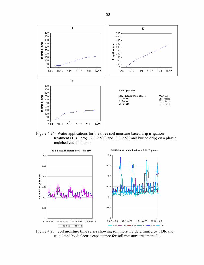
83
Figure 4.24. Water applications for the three soil moisture-based drip irrigation
treatments I1 (9.5%), I2 (12.5%) and I3 (12.5% and buried drip) on a plastic mulched zucchini crop.
Soil moisture determined from TDR
0
0.05
0.1
0.15
0.2
0.25
0.3
30-Oct-05 07-Nov-05 15-Nov-05 23-Nov-05
Soil
moi
stur
e (m
^3/m
^3)
TDR 51 TDR 52
Soil Moisture determined from ECH2O probes
0
0.05
0.1
0.15
0.2
0.25
0.3
30-Oct-05 07-Nov-05 15-Nov-05 23-Nov-05
I1-E4 I1-E5 I1-E6 I1-E7 I1-E8 I1-E9 Figure 4.25. Soil moisture time series showing soil moisture determined by TDR and
calculated by dielectric capacitance for soil moisture treatment I1.
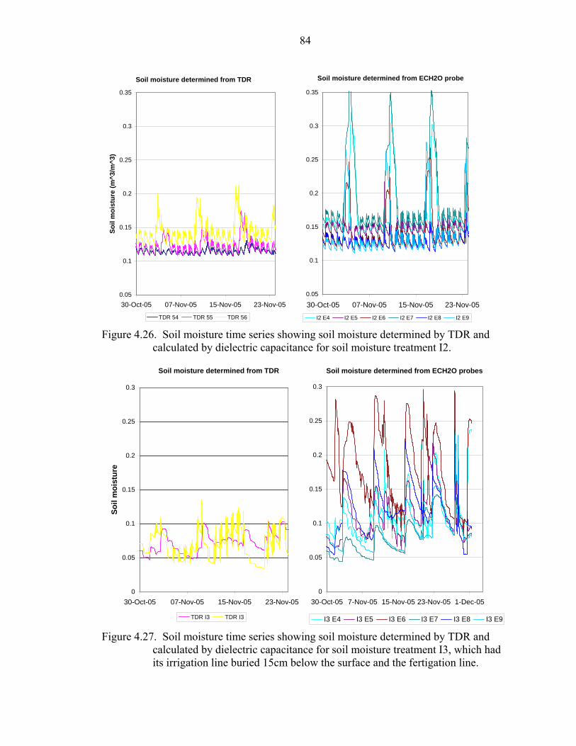
84
Soil moisture determined from TDR
0.05
0.1
0.15
0.2
0.25
0.3
0.35
30-Oct-05 07-Nov-05 15-Nov-05 23-Nov-05
Soil
moi
stur
e (m
^3/m
^3)
TDR 54 TDR 55 TDR 56
Soil moisture determined from ECH2O probe
0.05
0.1
0.15
0.2
0.25
0.3
0.35
30-Oct-05 07-Nov-05 15-Nov-05 23-Nov-05
I2 E4 I2 E5 I2 E6 I2 E7 I2 E8 I2 E9
Figure 4.26. Soil moisture time series showing soil moisture determined by TDR and calculated by dielectric capacitance for soil moisture treatment I2.
Soil moisture determined from TDR
0
0.05
0.1
0.15
0.2
0.25
0.3
30-Oct-05 07-Nov-05 15-Nov-05 23-Nov-05
Soil
moi
stur
e
TDR I3 TDR I3
Soil moisture determined from ECH2O probes
0
0.05
0.1
0.15
0.2
0.25
0.3
30-Oct-05 7-Nov-05 15-Nov-05 23-Nov-05 1-Dec-05
I3 E4 I3 E5 I3 E6 I3 E7 I3 E8 I3 E9
Figure 4.27. Soil moisture time series showing soil moisture determined by TDR and calculated by dielectric capacitance for soil moisture treatment I3, which had its irrigation line buried 15cm below the surface and the fertigation line.

85
If salinity was affecting mV readings, then this could go some way in explaining
the under application of water by the treatment. The probe would be recording mV and
thus soil moisture readings higher than actual conditions and the mV threshold, and
irrigation events would be bypassed. Salinity readings and effects are however not
quantified
Spatial distribution trends
The different spatial distributions of soil moisture showed that soil moisture
corresponded to emitter and plant position, but mostly was a function of distance from
the drip line. The curve fitted in Figure 4.20 suggests that the highest soil moisture
occurred near or at the drip line and that the lowest soil moisture occurred on the exterior
of the plant side of the bed. This initially seems intuitive, as one would expect the plant
to use up the available water and reduce the soil moisture on this side. The variability of
soil moisture readings was greatest near the emitters and also higher on the plant side of
the drip line (Figures, 4.14, 4.16 and 4.18). This is possibly due to the higher refilling
and consumption by the plant roots cycle in this region of the bed.
The distributions of soil moisture showed a fairly consistent band of high soil
moisture up to 10 cm on either side of the drip line, with highest values occurring near
the emitters. Variability in soil moisture showed a greater relation to emitter position and
plant position, than just distance to the drip line as soil moisture did. This is evident in
Figures 4.12, 4.14, and 4.18. To aid in the decision on probe placement and set point, the
soil moisture release curve and tensiometric distributions need to be considered. Due to
the particle distribution and hydrophobic nature of the sands, the soil moisture release
curve has a large change in slope between 12% and 8% soil moisture. For soil moistures
below 8% a small reduction in soil moisture can have a very large increase in soil

86
moisture tension. This is not conducive to optimal plant growth and these ranges of soil
moisture should be carefully avoided. This is evident in Figure 4.19, where the soil
moisture tension distribution increases dramatically beyond 20 cbar (approximately 15
cm either side of the drip line).
Conclusions
The dielectric capacitance probe was calibrated for the soil (fine sand) at the Plant
Science Research and Education Unit, as the probe needed site-specific calibration due to
the high sand content. The calibration yielded a linear relationship between soil moisture
and probe mV output, similar to that published for most soils by the probe manufacturers.
From this curve and tensiometric readings, a site-specific soil moisture release curve was
derived for the fine sand. The soil moisture release curve will help determine the plant
water stress that a crop may experience for particular soil moisture set points. This is
critical for optimal growth of the crop and ensuring that water is not a limiting factor
while achieving water application savings and reducing nutrient leaching.
Soil moisture within the plastic mulched bed is dependant on distance from the drip
line and emitters and to a much lesser extent distance from the plant. The average soil
moisture at a point in the bed can be estimated by a third order polynomial that is a
function of distance from the drip line. The curve is almost parabolic and skewed
slightly, possibly due to plant position within the bed. Soil moisture within the bed was
lowest on the outer side of the plants. Soil moisture variability was highest near the drip
emitters and lower towards the outer edges of the bed, where soil moisture use and
recharge by irrigation was almost neglegible. External factors such as rainfall and
temperature can have an effect on soil moisture readings. Rainfall generally did not
contribute substantially to soil moisture readings, but during significant rainfall events,

87
probes that were on the exterior of the bed and not protected by the crop canopy did
record increases of soil moisture up to 10% for large events. The trends were not clear,
and the effects of rainfall were random, and did not contribute to probe readings in the
center of the bed where probe’s should be positioned for soil moisture-based irrigation.
The dielectric capacitance probes are affected by temperature variations, but the soil has a
mediating effect on diurnal temperature fluxes and very little change in soil moisture
(less than 0.35%) is experienced when the probe is buried vertically in the top 22 cm of
the plastic mulched bed, for normal ranges of temperature in a growing season. As such
with good sealing for the probe in the plastic mulch, rainfall and temperature effects on
probe readings of soil moisture should be negligible. Soil moistures determined by
applying the linear calibration equation to dielectric capacitance probe mV output had
significant spikes corresponding to fertigation events that were not replicated in the TDR
measured soil moisture. The significant spikes in the dielectric capacitance data were not
caused by rainfall or temperature affecting the mV output. It is proposed that the
fertilizers added during fertigation events are increasing soil electrical conductivity, and
increasing the dielectric capacitance probes bulk conductivity reading and thus mV
output. If this is the case, then the dielectric capacitance probe needs to be calibrated for
higher salinity levels in sandy soils.
From this in field calibration and soil moisture spatial distribution study, it has been
shown that soil moisture measurements have inherent variability, and good understanding
of the factors affecting soil moisture within a plastic mulched bed on sandy soils is
needed to reliably schedule irrigation with soil moisture probes. Soil moisture
distributions show soil moisture profiles that correlate with proximity to the drip line and

88
emitters. Further studies should address the potential problems of high salinity effects
and the potential for integrating multiple probes into the systems operation.

90
CHAPTER 5 SUMMARY AND CONCLUSIONS
In the interest of promoting sustainability in agriculture the University of Florida
has developed a methodology of irrigation scheduling and a low cost technology to
implement the methodology. The technology has been tested on various locations,
seasons, soils and crops for its ability to be successfully applied to a wide range vegetable
production.
The system was applied to two plastic mulched tomato crops. The first experiment
was conducted in the winter, in South Florida, on a gravelly loam soil. The second
experiment was in North Central Florida, on fine sand in the spring of 2005. Both
experiment results showed significant water application savings of between 50 and 82%
can be achieved with the soil moisture-based irrigation scheduling compared to
traditional local grower practices that applied larger amounts of water less frequently.
For both experiments, soil moisture-based scheduling yields were equal to or above local
grower treatments, and this achieved irrigation water use efficiencies (IWUE) of between
216 and 415% greater. These reductions in water application are very significant for
many places in the world. In dry areas with water shortages, these high IWUE’s can
allow a grower to irrigate a larger area with the same water supply. Water savings can
also be very beneficial where water laws require expensive licenses to access resources.
In regions were power costs are high, lower water application combined with a well tank,
if feasible, can significantly reduce pumping costs and improve profit margins. Plastic
mulched beds combined with drip irrigation have significantly reduced disease incidence

91
by separating the fruit from the soil. Keeping the soil at optimal levels for plant growth
and avoiding over watering further helps reduce the changes for disease. In some cases
this was one of the reasons for the higher yields with the soil moisture-based scheduling
compared to the traditional time based scheduling. The incidence of disease had more
effect on yield for the wetter treatments. This may become a bigger factor as the
consumer market is becoming more aware of the use of chemicals to control diseases. In
Florida, water savings are also important in regions like South Florida. But, most
importantly the application of less water and the precision level of soil moisture control
have significant benefits for soil nutrient management.
Florida is a unique region. Nitrogen is typically the most important nutrient in
terms of limitations to growth and contamination to water resources in most places in the
world. Florida not only has nitrogen issues, but also and to an even greater extent,
phosphorous has become a major source for environmental imbalance and is the focus of
much work and restorative efforts. Although most of the excess phosphorous has been
introduced to the everglades system by the drainage of wetlands on exposure of the soil
to oxidation, agriculture has also contributed to water resource loading. The soil
moisture based-irrigation scheduling reduced total season loading of dissolved and total
phosphorous from plastic mulched tomatoes by between 65 and 71%. Higher reductions
(70-79%) were achieved during only the treatment period. From both experiments, the
reductions in nitrogen loading to local water resources were between 55 and 90% for both
nitrate and ammonia forms of nitrogen. Again reductions were higher if the
establishment period was excluded (70–97%). These reductions in nutrient leaching were
primarily driven by reductions in volumes of water passing through the root zone. The
total volume of leachate captured below the root zone in lysimeters was between 68 and

92
78% lower for the soil moisture-based treatments compared to the traditional time based
treatments. Between 73 and 85% less leaching by volume occurred during the treatment
period. One soil moisture-based irrigation treatment had its irrigation drip line buried 15
cm below the surface where its fertigation line was located. Water being applied below
the fertilizer application further reduced the concentration of nutrients in the leachate, and
thus over all nutrient loading.
Along with the reductions in nutrient loading, the system presents nutrient
management possibilities. Fertigation events can be automated which means less labor
requirements and precision nutrient applications to the crop. Different levels of
automation and different frequencies of fertilizer application through fertigation were
tested, namely; manual injection once a week using a peristaltic pump, automated
injection twice a week using a venturi injector controlled by the irrigation timer, and
continuous injection using a venturi injector that is driven by irrigation. Each method has
its pro and cons. The manual injection while being precise, required more labor and
higher capital layout for the pump. Extra labor was needed for both connection and
operation of the injection pump, and for measuring out and dissolving the fertilizer (if
dry) into solution. The continuous injection method required virtually no labor to operate
and a pre-dissolved or liquid solution of fertilizer was injected during each irrigation
event. This system required knowledge of the season’s water application so as to set the
concentration level in the tank from which injection takes place. For a time-based
schedule this is simple. For soil moisture-based scheduling a more empirical approach is
needed. Water requirements for the crop are dynamic and related to climatic conditions
and other growth factors. Previous experiments water applications using soil moisture-
based irrigation scheduling, were used as an estimate for water use for the coming season.

93
Crop type, season, location and soil moisture thresholds were also taken into
consideration. Fertilizer solution was thus calculated on the predicted water applications.
This was done for two experiments. The first experiments water application was very
close to the predicted amount and fertilizer application was similar to that intended for
the crop. The second experiment however had lower than expected water applications for
most of the season, partial due to colder than expected weather and reduced
evapotranspiration, and partially due to some incidence of disease. The fertilizer
application was thus lower than suggested and crop yield was slightly reduced. The same
could happen in reverse effect and there could be an over application of fertilizer if more
water than expected is applied. The third method of automated fertigation was not
dependant on irrigation, but retained its low labor benefits. At the cost 2 extra solenoid
valves, the system can be controlled by the irrigation timer on a separate schedule to the
irrigation. The injection is via a venturi injector and the fertilizer solution is still stored in
a tank to overcome the need to premix or measure out liquid fertilizer before each event.
Other benefits are that the system can run for a few minutes after the injection has
stopped to flush the line, and the fertigation frequency can also be user set. Optimal
fertigation frequency depends on the fertilizer used and the soil type. Other research has
found that higher frequencies are needed on sandy or coarse soils with low nutrient
holding capacity. For the two experiments conducted no increases in yield or growth
were found for the continuous or twice a week fertigation over the weekly manual events.
It can be concluded that no benefits for fertigation frequencies below a week are achieved
on the sandy soils tested. The automated independent fertilizer injection system is the
most recommended for the reasons above mentioned. Some considerations that may
cause a need for deviations from this system are, operating pressure and area fertigated.
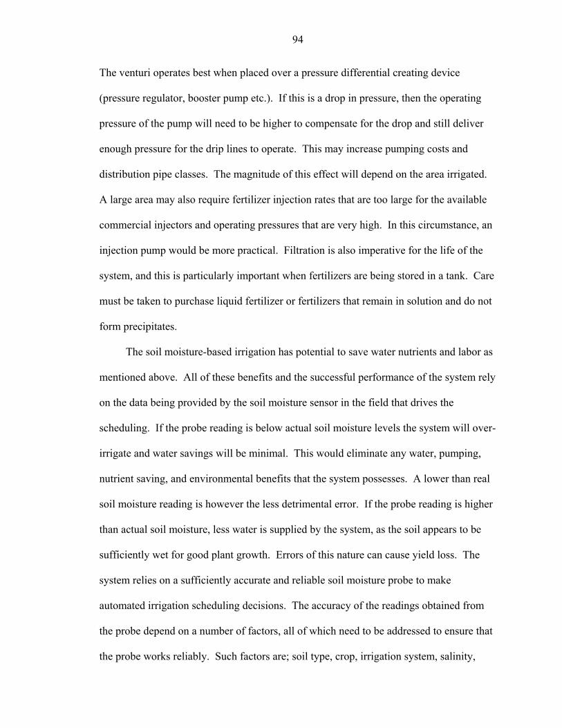
94
The venturi operates best when placed over a pressure differential creating device
(pressure regulator, booster pump etc.). If this is a drop in pressure, then the operating
pressure of the pump will need to be higher to compensate for the drop and still deliver
enough pressure for the drip lines to operate. This may increase pumping costs and
distribution pipe classes. The magnitude of this effect will depend on the area irrigated.
A large area may also require fertilizer injection rates that are too large for the available
commercial injectors and operating pressures that are very high. In this circumstance, an
injection pump would be more practical. Filtration is also imperative for the life of the
system, and this is particularly important when fertilizers are being stored in a tank. Care
must be taken to purchase liquid fertilizer or fertilizers that remain in solution and do not
form precipitates.
The soil moisture-based irrigation has potential to save water nutrients and labor as
mentioned above. All of these benefits and the successful performance of the system rely
on the data being provided by the soil moisture sensor in the field that drives the
scheduling. If the probe reading is below actual soil moisture levels the system will over-
irrigate and water savings will be minimal. This would eliminate any water, pumping,
nutrient saving, and environmental benefits that the system possesses. A lower than real
soil moisture reading is however the less detrimental error. If the probe reading is higher
than actual soil moisture, less water is supplied by the system, as the soil appears to be
sufficiently wet for good plant growth. Errors of this nature can cause yield loss. The
system relies on a sufficiently accurate and reliable soil moisture probe to make
automated irrigation scheduling decisions. The accuracy of the readings obtained from
the probe depend on a number of factors, all of which need to be addressed to ensure that
the probe works reliably. Such factors are; soil type, crop, irrigation system, salinity,

95
probe placement, cost and probe type. The ECH2O dielectric probes that has been tested
are well suited to coarse soils as it responds quickly to fast changes in soil moisture, are
suitable for most crops and irrigation systems as it can be buried at the required root
depth and averages the soil moisture reading over its 20 cm length, are low cost
compared to other dielectric probes, and can achieve accurate results for most soils
without calibration. The probe however does need calibration for sandy soils, and for
soils with high salinity. A calibration was thus carried out for the sandy soils at PSREU
where regular research is conducted on the soil moisture-based irrigation system. The
calibration was an in-situ calibration during a fall cropping season of zucchinis on plastic
mulched beds. Nesting tensiometeric, and TDR probes together with the ECH2O probes
gave simultaneous readings from which a linear soil moisture versus ECH2O probe mV
output was derived and a soil moisture release curve generated. The linear curve derived
for the ECH2O probe was
SM = 0.0006*mV – 0.1901
This is similar to the general curve that Decagon Devices Inc. (makers of the
ECH2O) provide for most soils. The 95% confidence intervals were also provided to
give an idea of the heterogeneity of the soil and probe dynamic.
The probe is sensitive to temperature and if temperature ranges are large and the
probe is buried at or near the surface, no real-time correction for the readings by the QIC
is currently available. From this study, it appeared that if the probe is buried vertically in
the top 20 cm of the soil in the plastic mulched bed, that temperature did not have any
significant effect. No diurnal flux in soil moisture readings were measured greater than
0.35%. This was for a difference in maximum and minimum temperature differential of
15 degrees Celsius. Temperature differences much larger than this are not common
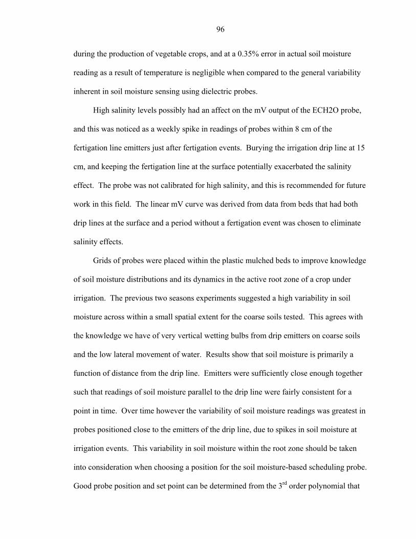
96
during the production of vegetable crops, and at a 0.35% error in actual soil moisture
reading as a result of temperature is negligible when compared to the general variability
inherent in soil moisture sensing using dielectric probes.
High salinity levels possibly had an affect on the mV output of the ECH2O probe,
and this was noticed as a weekly spike in readings of probes within 8 cm of the
fertigation line emitters just after fertigation events. Burying the irrigation drip line at 15
cm, and keeping the fertigation line at the surface potentially exacerbated the salinity
effect. The probe was not calibrated for high salinity, and this is recommended for future
work in this field. The linear mV curve was derived from data from beds that had both
drip lines at the surface and a period without a fertigation event was chosen to eliminate
salinity effects.
Grids of probes were placed within the plastic mulched beds to improve knowledge
of soil moisture distributions and its dynamics in the active root zone of a crop under
irrigation. The previous two seasons experiments suggested a high variability in soil
moisture across within a small spatial extent for the coarse soils tested. This agrees with
the knowledge we have of very vertical wetting bulbs from drip emitters on coarse soils
and the low lateral movement of water. Results show that soil moisture is primarily a
function of distance from the drip line. Emitters were sufficiently close enough together
such that readings of soil moisture parallel to the drip line were fairly consistent for a
point in time. Over time however the variability of soil moisture readings was greatest in
probes positioned close to the emitters of the drip line, due to spikes in soil moisture at
irrigation events. This variability in soil moisture within the root zone should be taken
into consideration when choosing a position for the soil moisture-based scheduling probe.
Good probe position and set point can be determined from the 3rd order polynomial that

97
describes soil moisture according to distance from the drip line, and soil moisture
variability.
Soil moisture based irrigation has proven to have high potential for water and
nutrient management. As resources become scarcer this methodology of irrigation could
become more and more vital for the survival of both growers, and the environment. For
the system to operate reliably and on a wide range of conditions, good knowledge of the
soil, probe and crop water requirements are essential. Further studies of issues that have
been highlighted are summarized here:
1. Integrating multiple probes into the QIC so that soil moisture readings are from two or more positions within the root zones of more than one plant. Multiple probe readings could be averaged or a median could be used to obtain a more representative measure of soil moisture within the bed, and reduce the potential for negative impacts of inherently heterogeneity in soils.
2. Test different methods of scheduling water to the transplant during the first two weeks of establishment. How is the soil moisture based irrigation system going to be applied to the small transplant with limited root systems? Can thresholds be changed to account for the limited root system? . Can more water savings be achieved in this period?
3. Test different crops, different micro irrigation systems, and different soils to get an indication of the systems application to a wide spread of conditions.
4. Calibrate the ECH2O probe’s response to salinity levels in sandy soils.
5. Measure temperature fluxes and corresponding probe readings at different depths and moisture contents, to evaluate the true impact temperature fluxes can have on the ECH2O probe.
6. Market, promote and continue the system research as a methodology and not a brand specific technology. Future success of the system requires the use of soil suitable probes, and good extension services to promote understanding of the systems operation to growers.
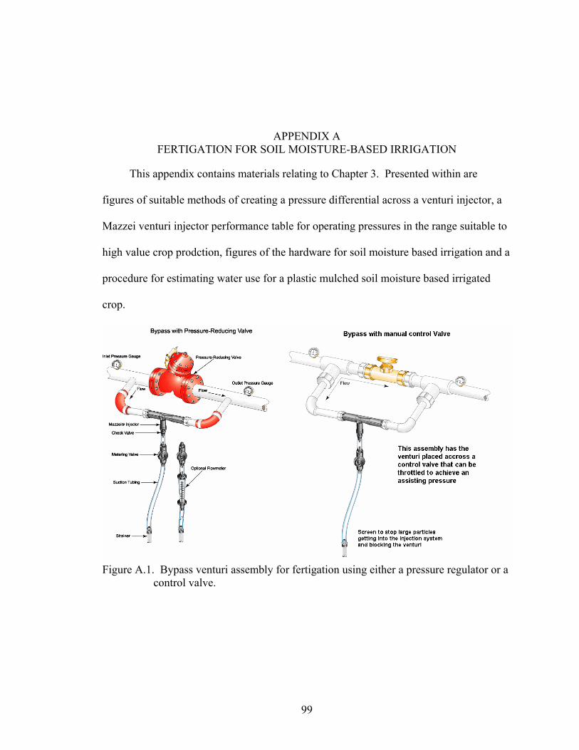
99
APPENDIX A FERTIGATION FOR SOIL MOISTURE-BASED IRRIGATION
This appendix contains materials relating to Chapter 3. Presented within are
figures of suitable methods of creating a pressure differential across a venturi injector, a
Mazzei venturi injector performance table for operating pressures in the range suitable to
high value crop prodction, figures of the hardware for soil moisture based irrigation and a
procedure for estimating water use for a plastic mulched soil moisture based irrigated
crop.
Figure A.1. Bypass venturi assembly for fertigation using either a pressure regulator or a control valve.

100
Figure A.2. Bypass assembly with a booster pump for venturi injection fertigation.
Figure A.3. Bypass assembly with venturi injector installed across an irrigation pump.
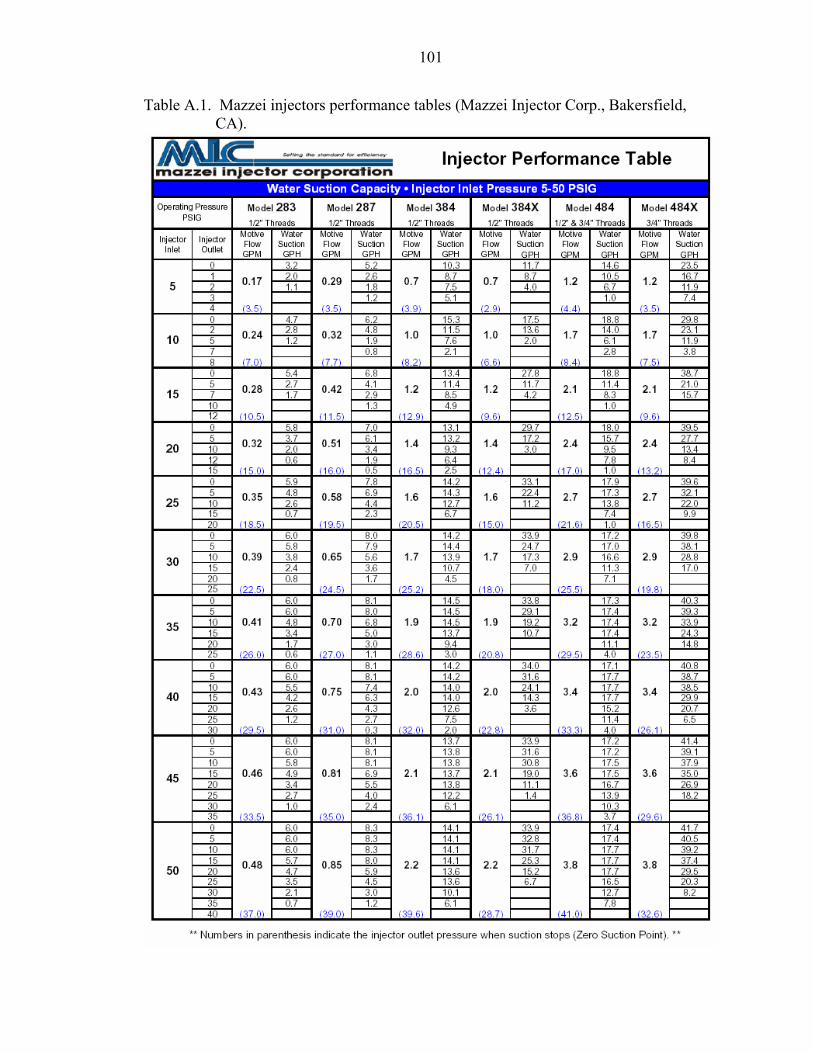
101
Table A.1. Mazzei injectors performance tables (Mazzei Injector Corp., Bakersfield, CA).
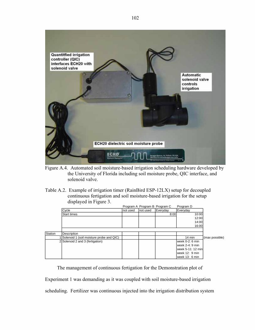
102
Figure A.4. Automated soil moisture-based irrigation scheduling hardware developed by the University of Florida including soil moisture probe, QIC interface, and solenoid valve.
Table A.2. Example of irrigation timer (RainBird ESP-12LX) setup for decoupled continuous fertigation and soil moisture-based irrigation for the setup displayed in Figure 3.
The management of continuous fertigation for the Demonstration plot of
Experiment 1 was demanding as it was coupled with soil moisture-based irrigation
scheduling. Fertilizer was continuous injected into the irrigation distribution system
Program A Program B Program C Program DCycle not used not used Everyday EverydayStart times 8:00 10:00
12:0014:0016:00
Station Description1 Solenoid 1 (soil moisture probe and QIC) 14 min (max possible)2 Solenoid 2 and 3 (fertigation) week 0-2: 6 min
week 2-4: 9 minweek 5-11: 12 minweek 12: 9 minweek 13: 6 min

103
every time irrigation occurred. The fertilizer applied was thus driven by the irrigation.
The complexity comes from the dynamic nature of soil moisture-based irrigation
scheduling which depends on the soil moisture characteristics of the soil, and the crop
evapotranspiration, which is driven by climatic conditions and crop growth stage. The
irrigation schedule will vary from season to season when using soil moisture as the basis
for scheduling. An estimate was needed to predict the water use for the crop over the
season. Crop evapotranspiration (ETc) is the IFAS recommended method for
determining water use. Previous experiments on tomatoes by Munoz-Carpena et al.
(2004) and (2005) reported consistent savings for two consecutive experiments in the
Miami-Dade County on tomatoes with the QIC and dielectric probe soil moisture-based
scheduling over the ETc schedule. The savings were 51% and 58% for two experiments
conducted during the winter seasons on Krome soil. Both these savings were recorded
for soil moisture tension thresholds of 15cbar. The threshold being employed on the
proposed experiment was 25 cbar and the higher value was likely to further increase
savings. The savings expected for the 25 cbar threshold were thus taken as 60%.
Although the total season water use expected was 60% lower, water use should still
follow the crop growth curve with low water requirements early in the season and higher
requirements once the crop is mature. The expected water use was thus determined by
reducing the ETc daily amount, which follows crop growth, by 60%. This can be seen in
Figure A.5.
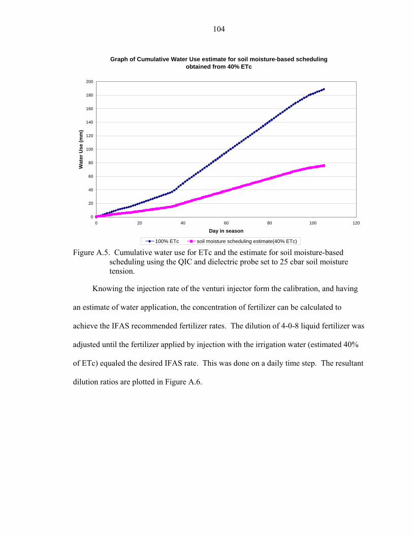
104
Figure A.5. Cumulative water use for ETc and the estimate for soil moisture-based scheduling using the QIC and dielectric probe set to 25 cbar soil moisture tension.
Knowing the injection rate of the venturi injector form the calibration, and having
an estimate of water application, the concentration of fertilizer can be calculated to
achieve the IFAS recommended fertilizer rates. The dilution of 4-0-8 liquid fertilizer was
adjusted until the fertilizer applied by injection with the irrigation water (estimated 40%
of ETc) equaled the desired IFAS rate. This was done on a daily time step. The resultant
dilution ratios are plotted in Figure A.6.
Graph of Cumulative Water Use estimate for soil moisture-based scheduling obtained from 40% ETc
0
20
40
60
80
100
120
140
160
180
200
0 20 40 60 80 100 120
Day in season
Wat
er U
se (m
m)
100% ETc soil moisture scheduling estimate(40% ETc)
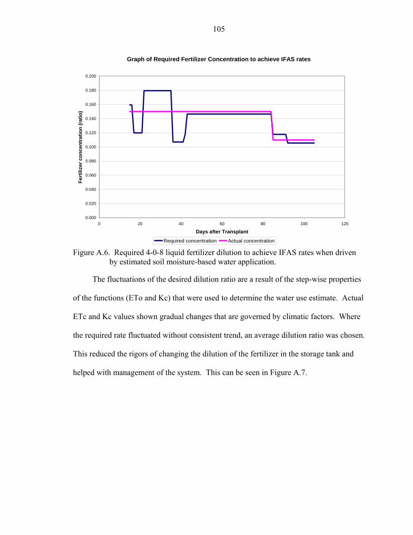
105
Figure A.6. Required 4-0-8 liquid fertilizer dilution to achieve IFAS rates when driven by estimated soil moisture-based water application.
The fluctuations of the desired dilution ratio are a result of the step-wise properties
of the functions (ETo and Kc) that were used to determine the water use estimate. Actual
ETc and Kc values shown gradual changes that are governed by climatic factors. Where
the required rate fluctuated without consistent trend, an average dilution ratio was chosen.
This reduced the rigors of changing the dilution of the fertilizer in the storage tank and
helped with management of the system. This can be seen in Figure A.7.
Graph of Required Fertilizer Concentration to achieve IFAS rates
0.000
0.020
0.040
0.060
0.080
0.100
0.120
0.140
0.160
0.180
0.200
0 20 40 60 80 100 120
Days after Transplant
Fert
ilize
r con
cent
ratio
n (r
atio
)
Required concentration Actual concentration
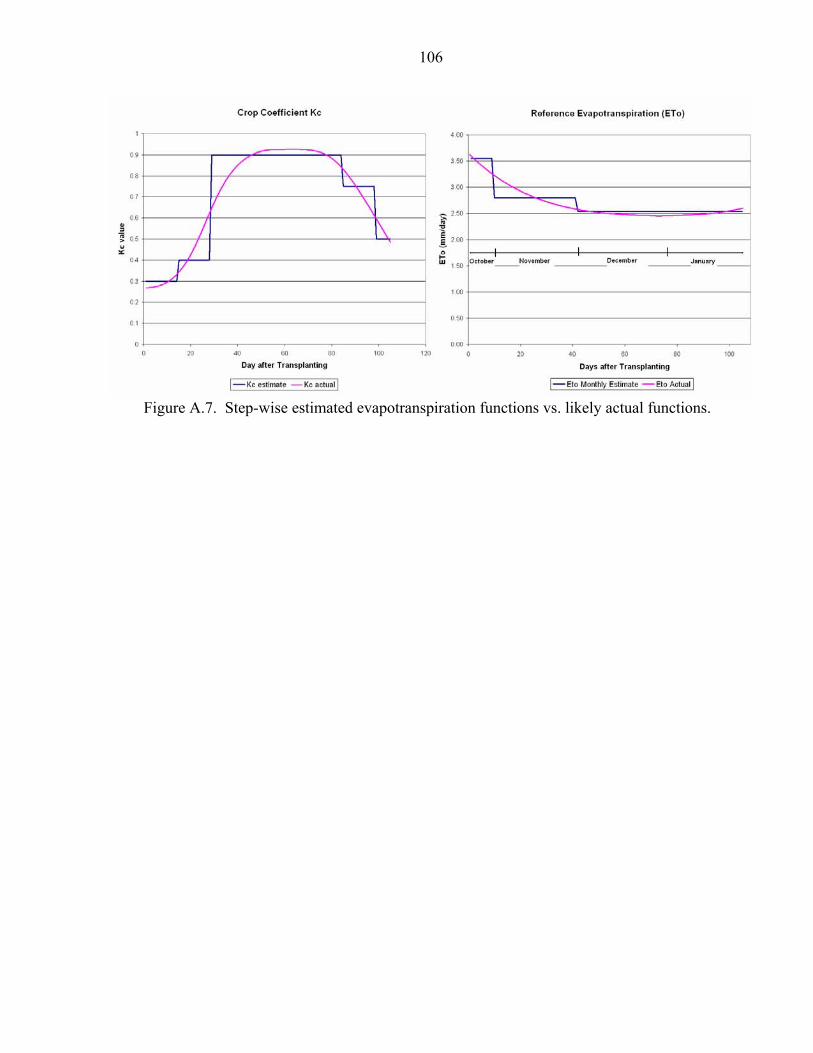
106
Figure A.7. Step-wise estimated evapotranspiration functions vs. likely actual functions.
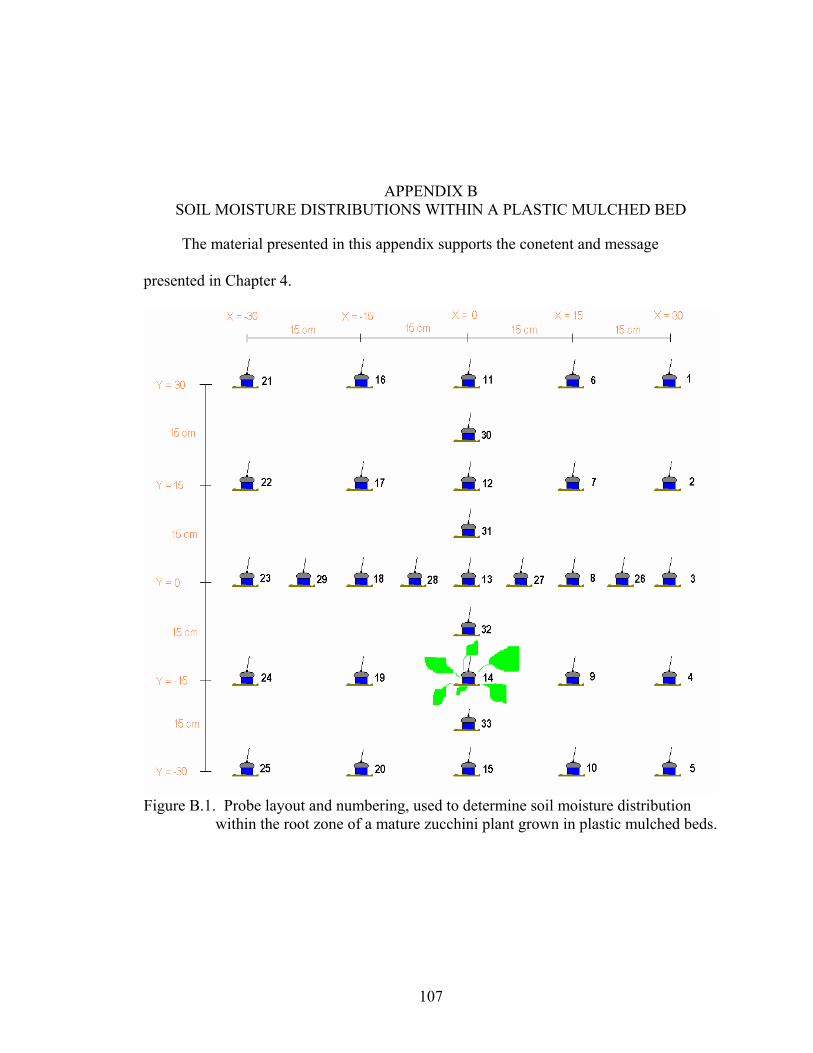
107
APPENDIX B SOIL MOISTURE DISTRIBUTIONS WITHIN A PLASTIC MULCHED BED
The material presented in this appendix supports the conetent and message
presented in Chapter 4.
Figure B.1. Probe layout and numbering, used to determine soil moisture distribution within the root zone of a mature zucchini plant grown in plastic mulched beds.
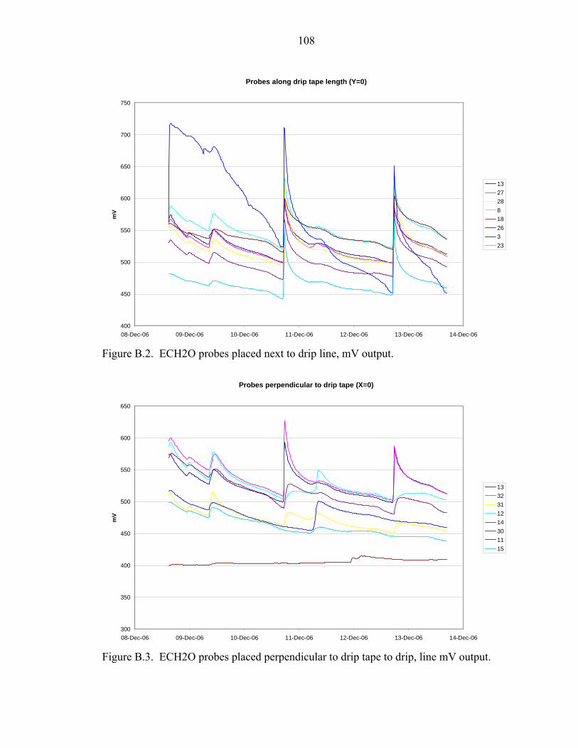
108
Figure B.2. ECH2O probes placed next to drip line, mV output.
Figure B.3. ECH2O probes placed perpendicular to drip tape to drip, line mV output.
Probes along drip tape length (Y=0)
400
450
500
550
600
650
700
750
08-Dec-06 09-Dec-06 10-Dec-06 11-Dec-06 12-Dec-06 13-Dec-06 14-Dec-06
mV
13272881826323
Probes perpendicular to drip tape (X=0)
300
350
400
450
500
550
600
650
08-Dec-06 09-Dec-06 10-Dec-06 11-Dec-06 12-Dec-06 13-Dec-06 14-Dec-06
mV
1332311214301115

109
Figure B.4. ECH2O probes parallel to and 30 cm from the drip line, mV output.
Figure B.5. ECH2O probes parallel to and 15 cm from the drip line, mV output.
Probes parrallel to drip tape (Y=15)
0
100
200
300
400
500
600
700
08-Dec-06 09-Dec-06 10-Dec-06 11-Dec-06 12-Dec-06 13-Dec-06 14-Dec-06
mV
27121722
Probes parrallel to drip tape (Y=30)
0
100
200
300
400
500
600
700
08-Dec-06 09-Dec-06 10-Dec-06 11-Dec-06 12-Dec-06 13-Dec-06 14-Dec-06
mV
16111621
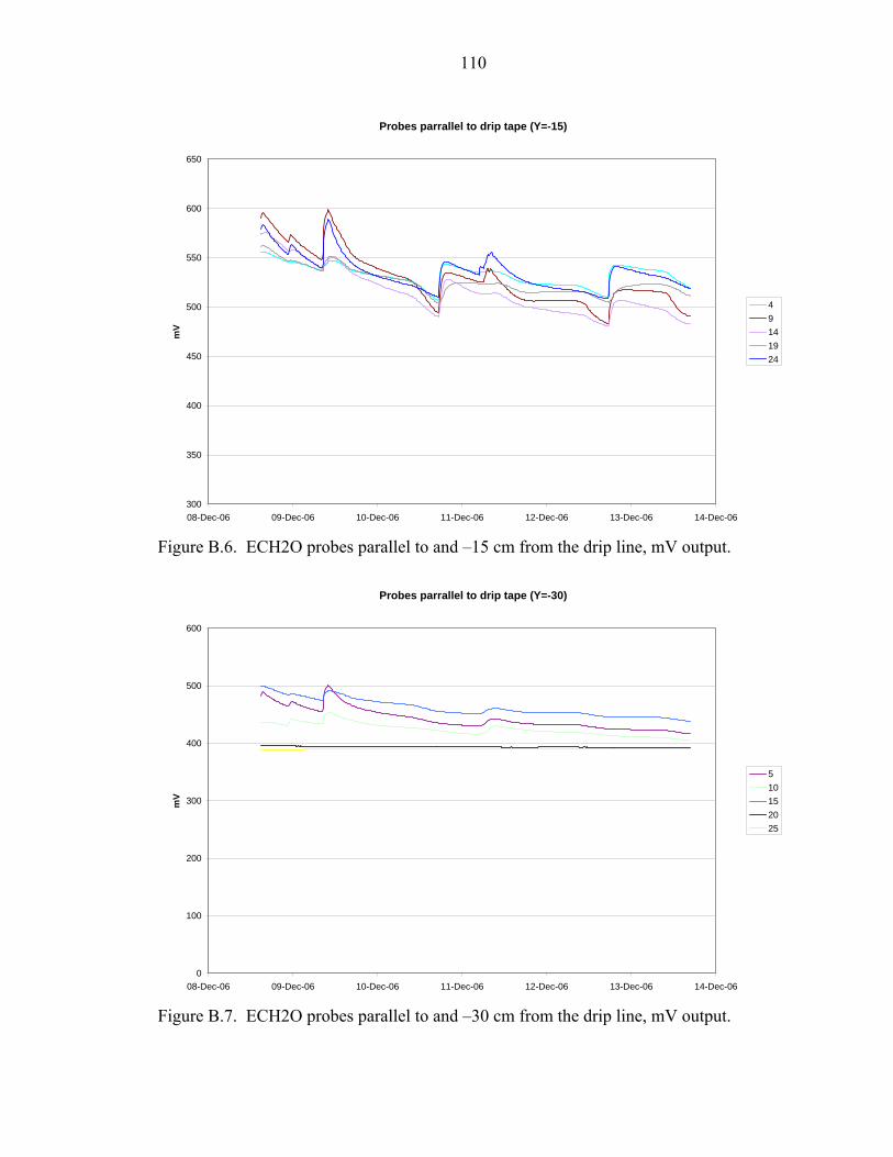
110
Figure B.6. ECH2O probes parallel to and –15 cm from the drip line, mV output.
Figure B.7. ECH2O probes parallel to and –30 cm from the drip line, mV output.
Probes parrallel to drip tape (Y=-15)
300
350
400
450
500
550
600
650
08-Dec-06 09-Dec-06 10-Dec-06 11-Dec-06 12-Dec-06 13-Dec-06 14-Dec-06
mV
49141924
Probes parrallel to drip tape (Y=-30)
0
100
200
300
400
500
600
08-Dec-06 09-Dec-06 10-Dec-06 11-Dec-06 12-Dec-06 13-Dec-06 14-Dec-06
mV
510152025

111
Figure B.8. ECH2O probes perpendicular to and 30 cm from the drip line, mV output.
Figure B.9. ECH2O probes perpendicular to and 15 cm from the drip line, mV output.
Probes perpendicular to drip tape (X=30)
0
100
200
300
400
500
600
700
800
08-Dec-06 09-Dec-06 10-Dec-06 11-Dec-06 12-Dec-06 13-Dec-06 14-Dec-06
mV
12345
Probes perpedicular to drip tape (X=15)
300
350
400
450
500
550
600
650
08-Dec-06 09-Dec-06 10-Dec-06 11-Dec-06 12-Dec-06 13-Dec-06 14-Dec-06
mV
678109
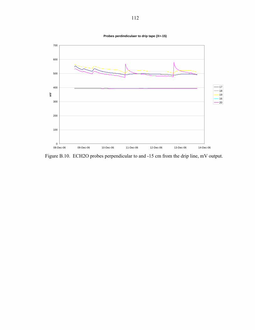
112
Figure B.10. ECH2O probes perpendicular to and -15 cm from the drip line, mV output.
Probes perdindiculaer to drip tape (X=-15)
0
100
200
300
400
500
600
700
08-Dec-06 09-Dec-06 10-Dec-06 11-Dec-06 12-Dec-06 13-Dec-06 14-Dec-06
mV
1718191620

113
LIST OF REFERENCES
Anonymous. 2005. ECH2O probe manual, Version 1.2. Decagon Devices Inc., Pullman, WA. Download literature, ECH2O products, manuals. http://www.ech2o.com/SupportDocumentation.htm last accessed 03/01/06.
Bauters, T.W.J., D.A. DiCarlo, T.S. Steenhuis, and J.Y. Parlange. 1998. Preferential Flow in Water Repellent Sands. Soil Science Society of America Journal 62 (5): 1185-1190.
Campbell, C.S. 2005a. Calibrating the ECH2O probes. Decagon Devices Inc., Pullman, WA. Download literature, ECH2O products, technical papers. http://www.ech2o.com/SupportDocumentation.htm lasted accessed 02/01/06.
Campbell, C.S. 2005b. Response of the ECH2O soil moisture probe to variations in water content, soil type and solution electrical conductivity. Decagon Devices Inc., Pullman, WA. Download literature, ECH2O products, technical papers. http://www.ech2o.com/SupportDocumentation.htm last accessed 02/27/06.
Campbell, C.S. 2005c. Response of ECH2O soil moisture sensor to temperature variations. Decagon Devices Inc., Pullman, WA. Download literature, ECH2O products, technical papers. http://www.ech2o.com/SupportDocumentation.htm last accessed 02/26/06.
Clark, G.A., C.D. Stanley, and D.N. Maynard. 1994. Tensiometer control vs. tomato crop coefficients for irrigation scheduling. ASAE Paper No. 94-2118. Amer. Soc. Agr. Eng., St. Joseph, Mich.
Clark, G.A., D.N. Maynard, C.D. Stanley, G.J. Hochmuth, E.A. Hanlon, and D.Z. Haman. 1990. Irrigation scheduling and management of micro-irrigated tomatoes. Fla. Coop. Ext. Serv. IFAS. University of Florida. Circ. 872.
Cook, W.P. and D.C. Sanders. 1991. Nirtogen application frequency for drip-irrigated tomatoes. Hortscience 26 (3): 250-252. Amer Soc Horticultural Science.
Dukes, M.D. and R. Muñoz-Carpena. 2005. Soil water sensor based automatic irrigation of vegetable crops. In: S. W. Trimble, B.A. Stewart and T.A. Howell (eds). Encyclopedia of water science. Marcel-Dekker, Inc : New York.
Dukes, M.D., E.H. Simonne, W.E. Davis, D.W. Studstill, and R. Hochmuth. 2003. Effect of sensor-based high frequency irrigation on bell pepper yield and water use, P. 665-674. In: Proc. 2nd Int. Conf. Irr. And Drainage, 12-15 May, Phoenix, Ariz.

114
Fares A. and AK. Alva. 2000. Evaluation of capacitance probes for optimal irrigation of citrus through soil moisture monitoring in an entisol profile. Irrigation Science 19 (2): 57-64 Jan 2000.
Florida Agricultural Statistics Service. 1995. Vegetable chemical use. 8pp. Fla. Agric. Stat. Serv., Orlando, FL.
Haddadin, S. H. and I. Ghawi. 1983. Effect of plastic mulches on soil water conservation and soil temperature in field grown tomato in the Jordan Valley. Dirasat 13(8): 25-34.
Hartz, T.K., and G.J. Hochmuth. 1996. Fertility management of drip-irrigated vegetables. UC Davis. Vegetable Research and Information Center.
Hebbar, S.S., B.K. Ramachandrappa, H.V. Nanjappa, and M. Probhakar. 2004. Studies on NPK drip fertigated field grown tomato. Europ. J. Agronomy 21: 117-127.
Herdel, K., P. Schmidt, R. Feil, A. Muhr, and U. Schurr. 2001.Dynamics in the concentrations and nutrient fluxes in the xylem of Ricinus communis-diurnal course, impact of nutrient availability and nutrient uptake. Plant, Cell and Env., 24:41-52.
Hochmuth G.J. 2000. Management of nutrients in vegetable production systems in Florida. Soil and crop science society of Florida proceedings 59:11-13. Soil Crop Science Florida.
Hochmuth, G.J., and A.G. Smajstrla. 1998. Fertilizer application and management for micro (drip)-irrigated vegetables in Florida. Fla. Coop. Ext. Serv. IFAS. University of Florida. Circ. 1181.
Hochmuth, G.J., and E.A. Hanlon. 1995. IFAS Standardized fertilizer recommendations for vegetable crops. Fla. Coop. Ext. Serv. IFAS. University of Florida. Circ. 1152.
Hoppula, K.I. and T.J. Salo. 2005. Tensiometer-based irrigation scheduling with different fertilizer methods in blackcurrant cultivation. ACTA Agriculturae Scandinavica, Section B-Soil and Plant Science 55(3):229-235 Sep 2005.
Howel, T. 2002. New ideas for improving irrigation water use efficiency. USDA Research Project Meeting: Irrigation methods, technology and management for increased water use efficiency. http://www.ars.usda.gov/research/publications/Publications.htm?seq_no_115=132922 last accessed 07/04/06.
Kukal, S.S, G.S. Hira, and A.S. Sidhu. 2005. Soil matric potential-based irrigation scheduling to rice (Oryza Sativa). Irri. Science 23(4):153-159.
Kutilek, M. and D.R. Nielsen. 1994. Soil hydrology. Catena Verlag, Cremligen-Destedt, Germany. Pp. 75-76.

115
Li, Y.C., Bryan, H.H., Klassen, W., Lamberts, M., and T. Olczyk. 2002. Tomato Production in Miami-Dade County, Florida. Fla. Coop. Ext. Serv. IFAS. University of Florida. Circ. HS858.
Locascio, S.J., G.J. Hochmuth, S.M. Olson, R.C. Hochmuth, A.A. Csizinsky, and K.D. Shuler. 1997. Potassium source and rate for polyethylene-mulched tomatoes. Hortscience 32 (7): 1204-1207.
Locascio, S.J., S.M. Olson, F.M. Rhoads, C.D. Stanley, and A.A. Csizinsky. 1985. Water and fertilizer riming for trickle irrigated tomatoes. Proc. Fla. State Hort. Soc. 98:237-239.
Lubana, P.P.S., and N.K. Narda. 1998. Soil water dynamics model for trickle irrigated tomatoes. Agricultural Water Management, 37:145-161. Elsevier Science.
Lyman Ott R., and M. Longnecker. 2001. An introduction to statistical methods and data analysis. 5th Edition. Duxbury, Thompson Learning.
Maynard, D.N., G.J. Hochmuth, S.M. Olson, C.S. Vavrina, W.M. Stall, T.A. Kucharek, S.E. Webb, T.G. Taylor, S.A. Smith, and E.H. Simonne. 2003. Tomato production in Florida. Chapter 41. In: S.M. Olson, and E. Simonne. Vegetable production guide for Florida 2003-2004. Fla. Coop. Ext. Serv. IFAS. University of Florida.
Morgan, K.T., L.R. Parsons, and T.A Wheaton. 2001. Comparison of laboratory- and field-derived soil water retention curves for a fine sand soil using tensiometric, resistance and capacitance methods. Plant and Soil, 234: 153-157.
Munoz-Carpena, R. 2004. Field devices for soil water content. Bull. 343. Fl. Coop. Extension Serv. IFAS, University of Florida, Gainesville.
Muñoz-Carpena, R. and M.D. Dukes. Design and field evaluation of a new controller for soil moisture-based irrigation. Submitted to Applied Engineering in Agriculture (Manuscript no. SW-06008-2005, August 2005).
Muñoz-Carpena, R., M.D. Dukes, L.W. Miller, Y.C. Li, and W. Klassen. 2004. Design and field evaluation of a new controller for soil moisture-based irrigation control. Unpublished draft for presentation in 2004 ASAE/CSAE Ann. Int. Meet., 1-4 Aug. Ottawa, Onario, Canada.
Muñoz-Carpena, R., M.D. Dukes, Y.C. Li, and W. Klassen. 2005. Field comparison of tensiometer and granular matrix sensor automatic drip irrigation on tomato. HortTechnology 15 (3)
Munoz-Carpena, R., Y.C. Li, and T. Olczyk. 2002. Alternatives of low cost soil moisture monitoring devices for vegetable production in south Miami-Dade County. Doc ABE 333. Fl. Coop. Extension Serv. IFAS, University of Florida, Gainesville.

116
Muñoz-Carpena, Y. Li, and T. Olczyk. 2002. Low cost moisture monitoring devices for vegetable production in the south Miami-Dade County agricultural area: Part 1-Alternatives. Fla. Coop. Ext. Serv. IFAS. University of Florida. ABE 333.
OI Analytical. @001. Nitrate plus nitrite nitrogen, USEPA by segmental flow analysis (SFA) or flow injection analysis (FIA). Publication 14900301. College Station, TX.
Qualls, R.J., J.M. Scott, and W.B. DeOreo. 2001. Soil moisture sensors for urban landscape irrigation Effectiveness and Reliability. Journal of the American Water Res. Ass. 37 (3): 547-559 Jun 2001.
Raskar, B.S. 2003. Effect of planting technique and fertigation on growth, yield and quality of banana (Musa sp). Indian Journal of Agronomy 48 (3): 235-237. Indian Soc Agronomy, Indian Agr Res Inst Div Agronomy, New Delhi 110012, India.
Scholberg, J., B.L. McNeal, K.J. Boote, J.W. Jones, S.L. Locascio, and S.M. Olson. 2000. Nitrogen stress effects on growth and nitrogen accumulation by field-grown tomato. Agr. Journal., Amer. Soc. of Agro, 92: 159-167.
Shae, J.B., D.D. Steele, and B.L. Gregor. 1999. Irrigation scheduling methods for potatoes in the northern Great Plains. Transactions of ASAE, 42 (2): 351-360 Mar-Apr.
Shock C.C., E.B.G. Feibert, and L.D. Saunders. 2000. Onion yield and quality affected by soil water potential as irrigation threshold. Hortscience 33 (7): 1188-1191 Dec.
Shock C.C., E.B.G. Feibert, and L.D. Saunders. 1998. Potato yield and quality response to deficit irrigation. Hortscience 33 (4): 655-659 Jul.
Simonne, E.H., M.D. Dukes, and D.Z. Haman. 2004. Principles and practices of irrigation management for vegetables. Chapter 8 in: Vegetable production guide for Florida 2003-2004. IFAS, Citrus and Vegetable Magazine.
Smajstrla, A.G and S.J. Locascio. 1994. Irrigation cutback effects on drip-irrigated tomato yields. Proc. Fla. State Hort. Soc., 107: 113-118.
Smajstrla, A.G. and S.J. Locascio. 1996. Tensiometer-controlled drip irrigation scheduling of tomato. Appl. Eng. Agr. 12: 315-319.
Smajstrla, A.G., D.S. Harrison, W.J. Becker, F.S. Zazueta, and D.Z. Hamon. 1985. Backflow prevention requirements for Florida irrigation systems. Fla. Coop. Ext. Serv. IFAS. University of Florida. Extension Mimeo Report 84-21 (revised).
Smajstrla, A.G., G.A.Clark, D.Z. Haman, and F.S. Zazueta. 1994. Design of agricultural irrigation systems in Florida. Fla. Coop. Ext. Serv. IFAS. University of Florida. Bul. 294.

117
Thompson T.L., S.A. White, J. Walworth, and G.J. Sower. 2003. Fertigation frequency for subsurface drip-irrigated broccoli. Soil Science Society of American Journal 67 (3): 910-918. Soil Sci Soc Amer, Madison, WI.
USEPA. 1993. Methods for the determination of inorganic substances in environmental samples. EPA/600/R-93/100. U.S. Gov. Print. Office, Washington, DC.
Wang, Q., W. Klassen, A.A. Abdul-Baki, H.H. Bryan, Y.C. Li, and M. Codallo. 2004. Influence of summer cover crops and irrigation rates on tomato yields and quality in a subtropical area. Proc. Fla. State Hort. Soc. 116: 140-143.
Zazueta, F.S., A.G. Smajstrla and G.A. Clark. 1994. Irrigation system controllers. Fla. Coop. Ext. Serv. IFAS. University of Florida. SS-AGE-22

118
BIOGRAPHICAL SKETCH
Born in South Africa in October 1981, Jonathan Schroder attended elementary and
high schools on the East Coast of South Africa near the City of Durban. He was awarded
academic honors and partook in multiple sports such as cricket, tennis, surfing and rugby.
He then attended the University of Natal (subsequently changed to the University of
KwaZulu Natal) where he achieved his bachelor’s degree in agricultural engineering cum
laude. After completing his undergraduate degree he accepted an offer to study for his
Master of Engineering, which has culminated in this document.