TVVR 10/5019

Soil Loss Estimation Based on the USLE/GIS

Approach Through Small Catchments

- A Minor Field Study in Tunisia

__________________________________________________________

Linus Andersson

Division of Water Resources Engineering Department of Building and Environmental Technology

Lund University

ii

Soil Loss Estimation Based on the USLE/GIS Approach Through

Small Catchments

A Minor Field Study in Tunisia

Linus Andersson

Avdelningen för Teknisk Vattenresurslära

TVVR-10/5019

ISSN-1101-9824

iii

Abstract

A USLE/GIS approach was applied to estimate soil loss for the two catchments ‘Mrichet’ and ‘Sadine2’ in

the semi-arid Tunisian Dorsal. The approach is inspired by the doctoral thesis ‘Water erosion modeling

using fractal rainfall disaggregation – A study in semiarid Tunisia’ by Dr. Sihem Jebari. The Universal Soil

Loss Equation (USLE) was applied to predict soil loss magnitude and Geographic Information System

(GIS) software ArcView and ArcMap was used to simulate the soil loss in spatial distribution. Each one of

the USLE-parameters (rainfall erosivity R, soil Erodibility K, topography LS, conservation practice P and

land use C) were represented by a thematic raster layer in the GIS. The thematic layers were defined

from available data such as satellite images (C and P), pedological maps (K), rainfall intensity records (R)

and topographic maps (LS). The model was calibrated primarily considering the grid cell size resolution

of the raster layers. The estimated soil loss was, depending on the grid cell dimension used, estimated at

approximately 12-16% of the observed soil loss for both catchments. The underestimation of the soil

loss is most likely due to underestimated K- and R-factor values. Also the USLE is restricted to rill and

inter rill erosion while the comparative observed erosion is likely to include all types of water erosion

within the catchment. This implies that the modeled values could be expected lower than the observed.

In addition some soil samples were analyzed and K-factor values experimentally determined for

comparison with the theoretical. These values were in the same order of magnitude as the theoretically

determined.

Keywords; USLE, Universal Soil Loss Equation, GIS, soil loss, erosion, water erosion modeling, Tunisia,

MFS, Minor Field Study

iv

v

Preface This project is part of my Master of Science degree in Environmental Engineering / Water Resource

Management at the Division of Water Resource Engineering (TVRL, LTH/Lund University). The project is

a combination of a literature review in the field of work and a simulation in soil loss estimation for two

smaller catchments in semiarid Tunisia. In addition to this also some field experiments are included.

Most of the literature review of this project is performed at Lund’s University, Sweden, while the

modeling phase (including construction of the model, field work and calibration)and the field work is

performed at the INRGREF (Tunisian National Research Institute for Rural Engineering, Water and

Forestry) research institute in Tunis, Tunisia. The study is supported by the Minor Field Study scholarship

from Swedish aid organization SIDA and is inspired by the doctoral thesis ‘Water erosion modeling using

fractal rainfall disaggregation – A study in semiarid Tunisia’ by Dr. Sihem Jebari at INRGREF, Tunis,

Tunisia, who also suggested the subject.

Supervisor for this project is Professor Ronny Berndtsson at TVRL, LTH / Lund University. Examiner is

Professor Kenneth M. Persson at TVRL, LTH/Lund University. The model work in Tunisia is supervised

and guided by Dr. Sihem Jebari at INRGREF, Tunis, Tunisia. Opponents are Kalle Koinberg and Patrik

Gliveson.

Acknowledgements

Very special thanks to Dr Sihem Jebari at INRGREF for her fine guidance and patience with my work.

Thank you Dr. Nejib Rejeb (head of INRGREF) for facilitating the cooperation with Lund University and

for providing all facilities for this work.

Also thank you Zaineb at INRGREF, professor Ronny at TVRL/LTH, Karin and Ulrik at GIS-centrum/Lund

University and Gerhard at Engineering Geology /LTH.

We are especially thankful to Mr. Mohamed Nasri (head of the Regional Agricultural Development

Department in Siliana), Mr. Jamel Ferchichi (head of the Farmland Conservation and Management

District) and Mr. Hammouda Aichi (head of the Soil District) and all other involved for helping us and

enabling us to perform experimental field work. Also great thanks to N.B. Awatef Abidi (managing the

soil lab), Neji and the other members of the staff who gave us a helping hand!

Finally a special thanks to the Jebari family (Omar, Walid) and Bouksila Fethi with family for taking care

of me during my stay. I would also like to mention coach Imed, coach Zied, Monsieur Trabelsi and all the

others at Federation de Boxe Tunisienne.

vi

Soil Loss Estimation Based on the USLE/GIS Approach Through Small Catchments

Abstract ................................................................................................................................................ iii

Preface ...................................................................................................................................................... v

Acknowledgements ............................................................................................................................... v

1. Introduction ...................................................................................................................................... 1

1.1. Background ............................................................................................................................... 1

1.2. Purpose ..................................................................................................................................... 1

2. Literature Review .............................................................................................................................. 3

2.1. Soil Erosion Processes ............................................................................................................... 3

2.2. Soil Erosion Related Problems .................................................................................................. 5

2.3. Universal Soil Loss Equation (USLE) .......................................................................................... 7

2.4. GIS and the USLE/GIS approach .............................................................................................. 11

3. Materials and Method .................................................................................................................... 15

3.1. Site presentation ..................................................................................................................... 15

3.2. Method.................................................................................................................................... 19

4. Results ............................................................................................................................................. 29

4.1. Soil Loss Estimation ................................................................................................................. 29

4.2. Field Work ............................................................................................................................... 32

5. Discussion ........................................................................................................................................ 34

5.1. Sources of Error –Generalizations, Approximations and Model Limitations .......................... 34

5.2. Conclusion ............................................................................................................................... 35

References .............................................................................................................................................. 37

Literature and Articles ........................................................................................................................ 37

Online .................................................................................................................................................. 38

Figures ................................................................................................................................................. 39

Appendix A – R-factor ............................................................................................................................. 40

Appendix B – Thematic layers ................................................................................................................. 47

Appendix C – Satellite Images ................................................................................................................. 55

1. Introduction

1.1. Background

In Africa it is estimated that the decrease in productivity due to soil erosion is 2-40% with an average of

8.2% for the whole continent (Eswaran et al, 2001). Also an average of 19% of the reservoir storage

volumes of Africa are silted (Jebari et al, 2009). In Tunisia in particular the problem is severe and has

been present for a long time with indications of measures taken against erosion thousands of years ago

by the Romans (Jebari 2009, FAO 1990, Toy et al 2002).

Every year 15 000 hectares of farming land is lost due to the erosion processes, affecting as much as

20% of the total land area of the country (Jebari, 2009). In a recent report concerning erosion and

siltation in Tunisia Jebari et al (2010) states that in the Tunisian Dorsal (the eastern parts of the Atlas

Mountains where the sites of this study are located) 7% of the land area is badly damaged by erosion

and as much as 70% moderately damaged, leaving only 28% of the Dorsal soil cover left. The situation is

an effect of thousands of years of agricultural activity in the area, but also to some extent short term

effects from dams built in the 60s and 70s have influenced the degradation. The main contribution of

the degradation is however the Mediterranean climate and conditions. The erosion effects are amplified

by the region soil structure being less developed; immature soils of rock origin with low organic content.

The high rates of weathering and erosion processes prevent soils from reaching maturity. Also

infiltration of water is decreased by shallow calcareous crust formations due to high evaporation rates

(Jebari et al, 2010) which in its turn accelerates the erosion processes.

The water demand in the Mediterranean region is now not far from the available resources and water is

becoming more expensive and more of a weight on the economy (Jebari et al, 2010). This obviously also

has a negative impact on the agricultural productivity, causing economical losses. It is therefore of great

importance to map these processes in order launch measures to control them. This project origins from

the doctoral thesis of Dr. Sihem Jebari, present at agricultural research institute INRGREF, Tunis, Tunisia;

‘Water erosion modeling using fractal rainfall disaggregation – A study in semiarid Tunisia’ (Jebari,

2009).

‘Water erosion modeling using fractal rainfall disaggregation – A study in semiarid Tunisia’ includes the

construction of a model that simulates the magnitude of soil loss in spatial distribution. Jebari states

that the main objective of her thesis is to develop a methodology for prediction of siltation (Jebari,

2009). This method used is called the USLE/GIS approach, which utilizes the empirical equation Universal

Soil Loss Equation (USLE) integrated in Geographic Information System (GIS) software. In her thesis, the

rainfall disaggregation for determination of the rainfall erosivity factor is the main focus.

1.2. Purpose

This project will give more focus on the general USLE/GIS approach for semiarid conditions, treating a

full construction of the model. The model will be derived from available data such as soil maps,

topographic maps, rainfall records, land use maps and satellite images. Finally the model is calibrated

and confirmed with siltation records observed in the modeled catchments. In addition, also some field

work will be performed to make comparisons with the theoretical values of soil properties.

2

The USLE/GIS-approach aims to generate a spatial distribution map describing the soil loss of the two

study sites. Interpretation of such a map will supposedly give the information required to take measures

to prevent potential erosion. However the main purpose of this project is oriented to applications of the

USLE/GIS approach for semiarid conditions in terms of methodology and calibration. Several similar

student projects are performed parallel at INRGREF under the supervision of Dr. Jebari; together the

results and conclusions of these will contribute to the development of erosion prediction technology for

semiarid conditions, where it is needed the most. In addition to the model work, this paper also contains

a literature review performed in the approach and in related processes in order to provide the reader a

basic introduction in the field and to understand the approach as it is used today.

3

2. Literature Review

2.1. Soil Erosion Processes

Earth landscape processes such as soil erosion and deposition have been active since the first rain fell

and the first wind blew millions of years ago, playing a significant role in the formation of these

landscapes (Toy et al, 2002). To understand the processes of erosion, it is also relevant to see it in its

context. Erosion processes are driven by the potential energy generated from tectonic activities inducing

the landscape cycle, raising and lowering the surface of the earth. The degradation of the landscape

works through four types of external processes: rock weathering, mass movement, erosion and

deposition (Toy et al, 2002). This chapter will treat a brief introduction on the basic functions of soil

erosion processes.

2.1.1. Soil Formation

Soil can be described as the earth surface top layer persisting of both mineral and organic material

(Strahler & Strahler, 2003). The structure and consistency of soils can vary widely. The mineral matter of

soils is the product of rock-weathering processes, while the organic matter content origins from

decomposition of biological matter (Strahler & Strahler, 2003). There are mainly two types of rock-

weathering processes; physical weathering and chemical weathering (Toy et al, 2002). Physical

weathering is decomposition of rocks into smaller fractures through various physical or mechanical

processes (Strahler & Strahler, 2003). The chemical weathering process is degradation of rocks due to

changes and decomposition in the mineral content (Toy et al, 2002). Examples of chemical weathering

processes are acid reactions, hydrolysis and oxidation reactions (Strahler & Strahler, 2003).

2.1.2. The Water Erosion Process

The type of erosion is generally classified by the erosive agent inducing the process; wind or water (Toy

et al, 2002). Water erosion can occur in many ways, for example coastal erosion by waves, splash

erosion from the impact of precipitation and irrigation water, erosion due to overland flow (also called

sheet erosion or rill/inter-rill erosion), stream channel erosion or erosion by percolating water (Strahler

& Strahler, 2003). Basically the impact of water droplets and/or the sheer stress caused by water in

motion detaches soil particles, followed by transport and finally deposition of the particles eroded

(Strahler & Strahler, 2003).

During storm events, rainfall intensity can exceed the infiltration capacity of the soil and the excess

water will form a runoff directed downslope (Toy et al, 2002). The magnitude of the runoff varies due to

different factors such as the initial soil moist, the infiltration capacity and the variations in precipitation

intensity (Toy et al, 2002). The moving water in the runoff and sub-surface flow naturally induces

erosion on the soil. The runoff will cause sheet erosion, which is more or less spatially uniform removal

of soil, or rill erosion which occurs in small closely related channels called rills (Strahler & Strahler, 2003;

Toy et al, 2002). With time rill erosion will progress to gully erosion as the channel increases in size and

is defined as a gully (Toy et al, 2002).

4

2.1.3. Soil erodibility

Many factors are important for the soils ability to resist erosion. The permeability is important since it

defines how the precipitation will be divided in terms of soil moisture, surface runoff and infiltrated

ground water (Toy et al, 2002). Also organic content is important; a higher organic content will decrease

the soil erodibility (FAO, 1996). As a high organic content increases the porosity and thereby also the

permeability and the water holding capacity of the soil, potential erosive runoff is reduced (Jankauskas

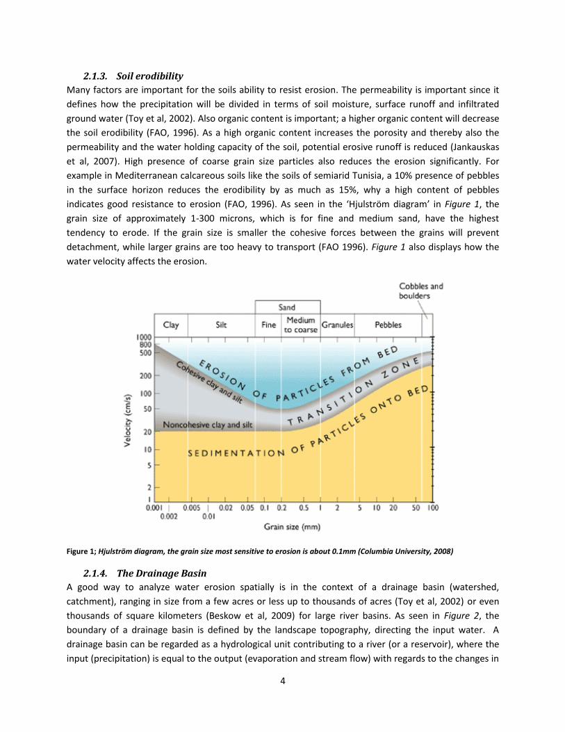
et al, 2007). High presence of coarse grain size particles also reduces the erosion significantly. For

example in Mediterranean calcareous soils like the soils of semiarid Tunisia, a 10% presence of pebbles

in the surface horizon reduces the erodibility by as much as 15%, why a high content of pebbles

indicates good resistance to erosion (FAO, 1996). As seen in the ‘Hjulström diagram’ in Figure 1, the

grain size of approximately 1-300 microns, which is for fine and medium sand, have the highest

tendency to erode. If the grain size is smaller the cohesive forces between the grains will prevent

detachment, while larger grains are too heavy to transport (FAO 1996). Figure 1 also displays how the

water velocity affects the erosion.

Figure 1; Hjulström diagram, the grain size most sensitive to erosion is about 0.1mm (Columbia University, 2008)

2.1.4. The Drainage Basin

A good way to analyze water erosion spatially is in the context of a drainage basin (watershed,

catchment), ranging in size from a few acres or less up to thousands of acres (Toy et al, 2002) or even

thousands of square kilometers (Beskow et al, 2009) for large river basins. As seen in Figure 2, the

boundary of a drainage basin is defined by the landscape topography, directing the input water. A

drainage basin can be regarded as a hydrological unit contributing to a river (or a reservoir), where the

input (precipitation) is equal to the output (evaporation and stream flow) with regards to the changes in

5

storage (Ward & Robinson, 2000). The flow of water in a drainage basin, oriented towards the “output

river”, can occur either as open channel flow in rills, gullies and stream channels, or as sub-surface flow

in the soil macro-pores (Toy et al, 2002).

Figure 2; The topography directs the precipitation and thereby defines the catchment borders.

2.1.5. Topography

Besides form defining the drainage basin limit, topography is a major factor influencing soil erosion

potential. Related to erosion processes, topography is described in terms of slope length (distance) and

slope steepness (ratio) and can be uniform (constant over the length), convex (increasing slope),

concave (decreasing slope) or a complex of these (Toy et al, 2002).

2.2. Soil Erosion Related Problems

Erosion act on land and inhabitants in many ways by changing the soil properties, bringing both

economical and social consequences on populations. Erosion related economical consequences in local,

regional and national scales can be derived from physical and chemical changes in the soil properties,

causing reductions in crop yields and requirements of increased efforts to maintain the agricultural

productivity (Toy et al, 2002). These problems are related to the changes in water holding capacity,

nutrient availability, reduction of organic matter content and general soil degradation (Toy et al, 2002).

Also siltation decreasing the water reservoir capacity is a great problem (Figure 3), especially in the

Mediterranean river basin (Jebari et al, 2010). A decreased reservoir also means less water for irrigation

and food supply as well as reductions in flood control. It has proven to be problematic to directly map

the relation of erosion to agricultural productivity due to the spatial and temporal variations of involved

conditions, but according to Toy et al (2002) erosion definitely affects this productivity in both short and

long term.

6

Figure 3; Silted reservoir in ‘Sadine2’ catchment in the Tunisian Dorsal. The reservoir has a capacity of 108 800 m3 and was

almost completely silted in approximately 10 years.

2.2.1. Erosion and Sediment Control

Sediment delivery can be reduced by reducing the waters sediment transport capacity, which in its turn

is reduced by a lower water velocity. But as seen in the ‘Hjulström diagram’ (Figure 1) this will primarily

cause a deposition of coarse grained particles, which reduces the pollution potential in the runoff less

than it reduces the total delivery of sediments, all because the fine sediments cause a more extensive

degradation of water quality and can also carry adsorbed pollutants like chemicals (Toy et al, 2002).

Therefore the best way to apply water and soil conservation practices is to protect the soil by reducing

detachment – only reducing the water sediment transport capacity will just cause a selection of eroded

particles; coarse particles will be left behind in the soil and pollution will be retained in the runoff (Toy

et al, 2002).

Toy et al (2002) describes some basic concepts for erosion-control principles. Some important

conservation practices are listed below;

- Maintain vegetation/ground cover; erosion is reduced by the ground cover providing canopy

that intercepts the rainfall and thereby reduces its erosivity. Ground cover from plant litter also

contributes and root networks improves soil fixation. Plant litter is preferably maintained for the

period of highest rainfall erosivity (if not possible for the whole year).

- Add support practices such as banquettes, terraces, vegetation strips, strings of rock and

armored waterways to reduce erosion in steep slopes. Ridging or contouring perpendicular to

the runoff is also a good measure.

- Modify the topography to avoid convexity at the end of slopes. Flat and concave segments at

the end of a slope are preferred to induce deposition.

- Incorporate biomass (manure, sewage sludge, paper mill waste) into the soil; as mentioned in

2.1.3 Soil Erodibility, the erodibility is reduced with increased organic matter content in the soil.

Also the litter of last year’s crop will contribute to higher organic matter content.

7

- Crop rotation – if a crop is sensitive to erosion it can be cultivated in rotation with another crop

with less erosive attributes to improve the overall influence.

Figure 4; ´String of rock´ conservation measure by the Tunisian Ministry of Water and Soil Conservation. The landowner

improves the ridge by planting cactuses to consolidate the structure.

An example of conservation measures in semiarid Tunisia is these stone ridges (Figure 4). Initially a

string of rock is founded by the Tunisian Ministry of Water and Soil Conservation. Then the landowner

continues the work by consolidating the structure with soil and adding pieces of cactus, intended to root

(Figure 4A). Eventually the cactuses will grow and form a vegetated rock strip, consolidated with cactus

roots and deposited soil, effectively stopping the runoff and eroded sediments can be deposited (Figure

4B).

2.3. Universal Soil Loss Equation (USLE)

The simplest mathematical model for prediction of soil loss is the Universal Soil Loss Equation (USLE) and

has been frequently used over the world since it was developed by American statistician W. H.

Whichmeier in the 1960s (Fistikogli & Harmancioglu 2002, USDA/NSERL 2010). The model is empirical

and was developed using over 10,000 statistical records of erosion, sampled over the American Great

Plains (FAO 1996). In fact the USLE is the most widely used equation in erosion modeling (Fistikogli &

Harmancioglu 2002).

8

The USLE describes average annual soil loss rates based on estimated and measured input data. The

input data is divided into five different factors; rainfall erosivity, soil erodibility, topography, crop

management and conservation practice. The factors of the USLE vary over different storm events but

tend to average out over long-term conditions, why the equation is applicable in these actual conditions

(Fistikogli & Harmancioglu 2002).

2.3.1. Equation Parameters

The annual soil loss A from the USLE (eq.1) is a mathematical product of the input parameters shown in

Table 1, given in ton per hectare and year.

PCLSKRA (eq.1)

Table 1; The USLE input factors with units where ‘MJ’ is megajoule, ’mm’ millimeters, ‘ha’ hectares, ‘h’ hours, ‘yr’ years and ‘t’

tons (Beskow et al, 2009).

Parameter Unit

R=rainfall erosivity factor

yrhha

mmMJ

K=soil erodibility factor

mmMJ

ht

LS= topographical factor (length, slope) -

C=crop management factor -

P=conservation practice factor -

2.3.1.1. Rainfall Erosivity Factor (R)

The contribution of the erosive agent water (precipitation) is represented by the rainfall erosivity factor

R. This factor is may be the most important factor in the USLE compared to the other input parameters

(Jebari, 2009). The kinetic energy of the rain can be considered as the potential rainfall energy available

to be transformed into erosion. The erosivity of a single raindrop is naturally described as the droplet

kinetic energy E; the mass of the droplet multiplied by the square of the velocity at impact divided by

two; E=mV2/2 (Toy et al, 2002). The R-factor corresponds to this kinetic energy E of the rainfall,

multiplied by the maximum intensity of a 30-min rain I30 according to the original approach by

Whichmeier (FAO, 1996), however Jebari et al (2008) found that using 15-min periods for the maximum

rainfall intensities could be more suiting for semiarid regions. The R-factor is calculated over long term

conditions (20 years) for all storm events with a precipitation exceeding 12,7 mm. Then an annual

average is deduced from this (FAO, 1996). According to the original approach by Whichmeier two valid

storm events must be separated by a minimum of six hours (OMM/WCP, 1983). An extensive example of

9

R-factor determination according to the Whichmeier methodology for a single event is found in

Appendix A.

2.3.1.2. Soil Erodibility Factor (K)

The soil erodibility factor can be described as the soils tendency to erode. It is dependent on the local

soil properties and can be determined in various ways; through sample analysis of the soil, from a soil

map or pedological survey of the site or through a combination of these (Jebari, 2009; Fistikogli &

Harmancioglu, 2002). Two energy sources are considered to erode the soil and the erodibility factor is

defined by the soil ability to resist these sources; the surface impact of the rain droplets and the

shearing stress of the horizontal runoff (FAO 1996). Whichmeier determined the main attributes for the

soil erodibility factor with experimental plots with both simulated and natural rain under specific

conditions; 22 meter plot length, 9% plot slope, no organic matter ploughed in for three years and

cultivation of the plot in the direction of slope (FAO, 1996). Whichmeier found that the main attributes

of the soil for determining the K-values were organic matter content, texture, surface horizon structure

and the permeability.

When determining the K-factor by sample analysis the following data is determined (Roose, 1989);

- The percentage of silt and fine sands; grain sizes 0.002 mm – 0.100 mm

- The percentage of sands; grain sizes 0.100 mm – 2 mm

- The percentage of organic matter content

- The soil structure class where the aggregate durability is considered; 4 classes are used

- The soil permeability class; 6 classes are used

Then the diagram of Figure 5 is used to deduce the K-factor value in US-units. In the example shown

below the sample contains 65% silt and fine sand, 5% sand, 2.8% organic matter content, class 2 in soil

structure and class 4 in permeability. The K-value is determined to 0.31, which can be converted to SI-

units by conversion factor KSI = 0.1317KUS (Zante et al, 2001).

10

Figure 5; Determination of K-factor value from soil sample analysis (FAO, 1996b).

2.3.1.3. Topographic Factor (LS)

Slope gradient and slope length are normally combined into one single factor in the USLE. This factor can

be calculated in various ways depending on unit preferences and other conditions like available data.

Different empirical relations are used to determine this factor and many recent studies (Jebari, 2009;

Onyando et al, 2004) use the equation (eq. 2) recommended by Morgan and Davidson (1991) where L is

the slope length in meters and S is the slope steepness in percent.

20065.0045.0065.022

SSL

LS (eq. 2)

Another common method also found in recent articles (Jain et al, 2010; Beskow et al, 2009; Erdogan et

al, 2006) is the theoretical relations of the unit stream power theory (eq. 3) (Moore et al, 1986a, 1986b,

1992) where AS is the upslope contributing area (taking accumulated flow of sediment and water into

consideration) and is the slope in degrees.

11

3.14.0

0896.0

sin

13.22

SALS (eq. 3)

2.3.1.4. Crop Management (C) and Conservation Practice (P) Factors

The C-factor describes the relation between the erosion on bare soil and the erosion on cropped

conditions. It is also called the ‘plant cover factor’ (FAO, 1996). In theory it will adopt a value of 1 for

completely unprotected, bare soil (which means no influence on gross erosion estimation) and for more

erosion reducing plant cover the value decreases, giving a lower estimation on gross erosion (FAO,

1996). For example an area with light forest vegetation will be assigned a value of 0.10 (Zante et al,

2001).

The P-factor represents erosion reducing measures like terraces or ridging/contouring. The P-factor is

assigned the value of 1 when no influences from conservation practices are considered. If conservation

measures are taken the value will decrease and thereby lower the estimated erosion (FAO, 1996). For

example a banquette on a 5-10% slope will give a P-factor value of 0.10 (Zante et al, 2001).

2.3.2. Limitations

Being the most widely used equation in erosion prediction, the USLE still has limitations and

weaknesses;

- The USLE in its original form does not model erosion in a spatial context; however this limitation

is overcome when integrated with GIS (Fistikogli & Harmancioglu, 2002).

- Deposition is not included in the USLE. Nor does it model wind-, mass-, tillage-, channel- or gully

erosion, it is developed to simulate inter-rill and rill erosion (sheet and rill erosion) (Fistikogli &

Harmancioglu 2002, FAO 1996, Stone & Hilborn 2000).

- Also the interaction between factors is not taken in consideration. For example the influence of

the equation factors from a slope with a specific vegetation cover and a characteristic soil type

are applied separately and do not interact (FAO 1996). This means that a potential synergy or

side effect of combined conditions may be lost.

- Finally the equation is only valid for long term conditions, why it is not valid to simulate the

effects of individual storms (FAO 1996).

2.4. GIS and the USLE/GIS approach

As mentioned in chapter 2.3, the non-existing spatial distribution of the USLE is overcome by integration

with GIS. In fact the USLE is a very powerful tool when integrated with GIS, especially for the conditions

in developing countries where lack of data rule out reliable applications of more advanced, physically

based models (Beskow et al, 2009). The simplicity of the USLE is most likely the main reason why it is still

widely used where data is insufficient.

12

2.4.1. Concept of the model

A GIS is not restricted to display and edit digital maps, other data can be stored and related to a position

or object as well. Thematic layers can represent data elements in the GIS – for example maps of

topography, geology, soils and precipitation as well as information on population and archaeology etc.

(Figure 6) (Larsson & Harrie, 2005).

Figure 6; Principle of the thematic layers in a GIS (Larsson & Harrie, 2005)

In order to apply the USLE in a GIS, every parameter is organized as a thematic layer which is providing a

spatial distribution. The layers need to be of the type ‘raster’, which means that they are in the form of

grid nets (matrixes). In the spatial distribution of the raster, every grid cell has a unique parameter value

and the model is executed by an overlay operation that multiplies all the parameter layers

mathematically. This means that every single cell is overlaid (multiplied) with its spatially corresponding

cells in the other parameter layers, completing the multiplication of the equation. The output of the

model is a combined layer where every single cell value is the product of the equation. Finally the whole

layer is summed and the average annual soil loss per hectare is calculated by taking the total catchment

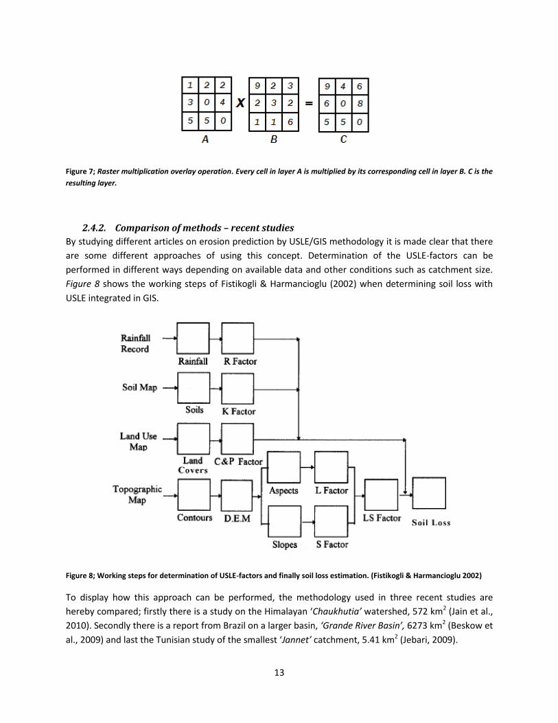
area in consideration. An example of the overlay operation is displayed in Figure 7, where ‘C’ is the

output raster when ‘A’ and ‘B’ is overlaid by multiplication.

13

Figure 7; Raster multiplication overlay operation. Every cell in layer A is multiplied by its corresponding cell in layer B. C is the

resulting layer.

2.4.2. Comparison of methods – recent studies

By studying different articles on erosion prediction by USLE/GIS methodology it is made clear that there

are some different approaches of using this concept. Determination of the USLE-factors can be

performed in different ways depending on available data and other conditions such as catchment size.

Figure 8 shows the working steps of Fistikogli & Harmancioglu (2002) when determining soil loss with

USLE integrated in GIS.

Figure 8; Working steps for determination of USLE-factors and finally soil loss estimation. (Fistikogli & Harmancioglu 2002)

To display how this approach can be performed, the methodology used in three recent studies are

hereby compared; firstly there is a study on the Himalayan ‘Chaukhutia’ watershed, 572 km2 (Jain et al.,

2010). Secondly there is a report from Brazil on a larger basin, ‘Grande River Basin’, 6273 km2 (Beskow et

al., 2009) and last the Tunisian study of the smallest ‘Jannet’ catchment, 5.41 km2 (Jebari, 2009).

14

The K-factor was derived and digitized from soil maps, national geological surveys and classifications in

literature in all three studies (Jebari, 2009; Beskow et al., 2009; Jain et al, 2010). Beskow et al (2009)

mentions that actual field measurements would be to expensive and time consuming while Jebari (2009)

has used complementary field work in addition to available data.

For the LS-factor, Jebari (2009) has used a DEM (Digital Elevation Model) derived from a topographical

map with a vertical resolution of 10 meters, scaled at 1:50000. A constant slope length L, set to 15

meters, was used over the whole catchment and then the LS- factor was calculated for slopes classified

in three classes using the equation (eq. 2) recommended by Morgan and Davidson (1991) (Jebari, 2009).

Jain et al (2010) used a 50 m grid cell resolution for the DEM, derived from a map scaled at 1:50 000

interpolated in the GIS-software. The LS-factor was determined with the equation from the theoretical

relations of the unit stream power theory (eq. 3) (Moore et al, 1986a, 1986b, 1992) “as this relation is

best suited for integration with GIS” (Jain et al, 2010). Beskow et al (2009) used a similar (eq. 3) relation

as Jain et al for LS, with some minor changes in the approach, using different categories for different

slopes and changing equation constants regarding to slope steepness. L and S were determined

separately using a 30 m grid size resolution for the DEM. The L-factor was derived from a fixed field

slope length equal to the grid cell size (30 m) for three categories of slope; 0-3%, 3-5%, +5%. The S-factor

was determined separately for two categories; 0-9% and +9%. In the study of Beskow et al (2009) the

slopes were generally steep with a 17.21% average.

Concerning the R-factor, both Jebari (2009) and Jain et al (2010) used a constant R-factor value for the

entire catchment. Beskow et al (2009) used six rainfall gauges evenly spread over the catchment. The

GIS-tool was used to determine the representation of each station in terms of catchment area, resulting

in a thematic layer for the R-factor.

Determination of the P- and C-factor for the Jannet catchment was performed through interpretation of

aerial photos at scale 1:20000, having both factors divided into six classes (Jebari, 2009). In the

Chaukhutia watershed, satellite images geo-coded at 30m pixel cell resolution where used for

determination of the C-factor, divided into six classes (Jain et al, 2010). The P-factor was assumed to be

homogenous and estimated to 0.7 for the entire catchment (Jain et al, 2010). Beskow et al (2009)

considered the entire Grande River Basin unaffected by conservation practices, why the P-factor was set

to 1.0. The C-factor map for the Grande River Basin was developed based on previous Brazilian studies,

derived from satellite images into six classes (Beskow et al, 2009).

15

3. Materials and Method

3.1. Site presentation

The two catchments studied are ‘Sadine2’ and ‘Mrichet’, located in north-central Tunisia in the Dorsal -

Mountains (the easternmost parts of the Atlas chain) (Figure 9). The highest peak of the Dorsal is at

1,544 m above sea level and the mountains cover an area of 12,490 km2. The Dorsal is located within the

400 mm/year precipitation isohyet, which is considered the limit for agriculture (Jebari, 2009). The two

studied catchments are included and monitored in the EU-funded HYDROMED-project, covering a total

of approximately 30 small experimental reservoirs in the Dorsal, for which precipitation is recorded

(Jebari, 2009).

Figure 9; Location of the studied catchments, ‘Mrichet’ and ‘Sadine2’ (Jebari, 2009)

16

3.1.1. Mrichet

Mrichet catchment (Figure 10) has an area of 1.58 km2 (158ha) of which 92% is agricultural land

(Convention CES/IRD, 1996-2002). Elevation ranges within 140 meters and the average slope is 11.1%

(Jebari et al, 2010). The reservoir of Mrichet was constructed in 1991 and holds a total volume of 42 400

m3 of which 22.7 % (9 610 m3) was silted at the last measurement, 1999-09-24 (Convention CES/IRD,

1996-2002). No date is given for installation of a detailed automatic precipitation recording device,

however records are available from 1993-09-24 to 2002-09-25. The average long-term precipitation

(1969-1998) is about 407 mm/yr with a standard deviation of 121 mm/yr (Figure 11). The observed

average annual soil loss Aave is 11.4 ton ha-1 yr-1 (recorded from 1991 to 1999) and the observed

maximum annual soil loss Amax is 19.5 ton ha-1 yr-1 (recorded 1996-05-29 to 1998-03-17).

Figure 10; The hydrological network of ‘Mrichet’

17

Figure 11; Long-term precipitation records of ‘Mrichet’

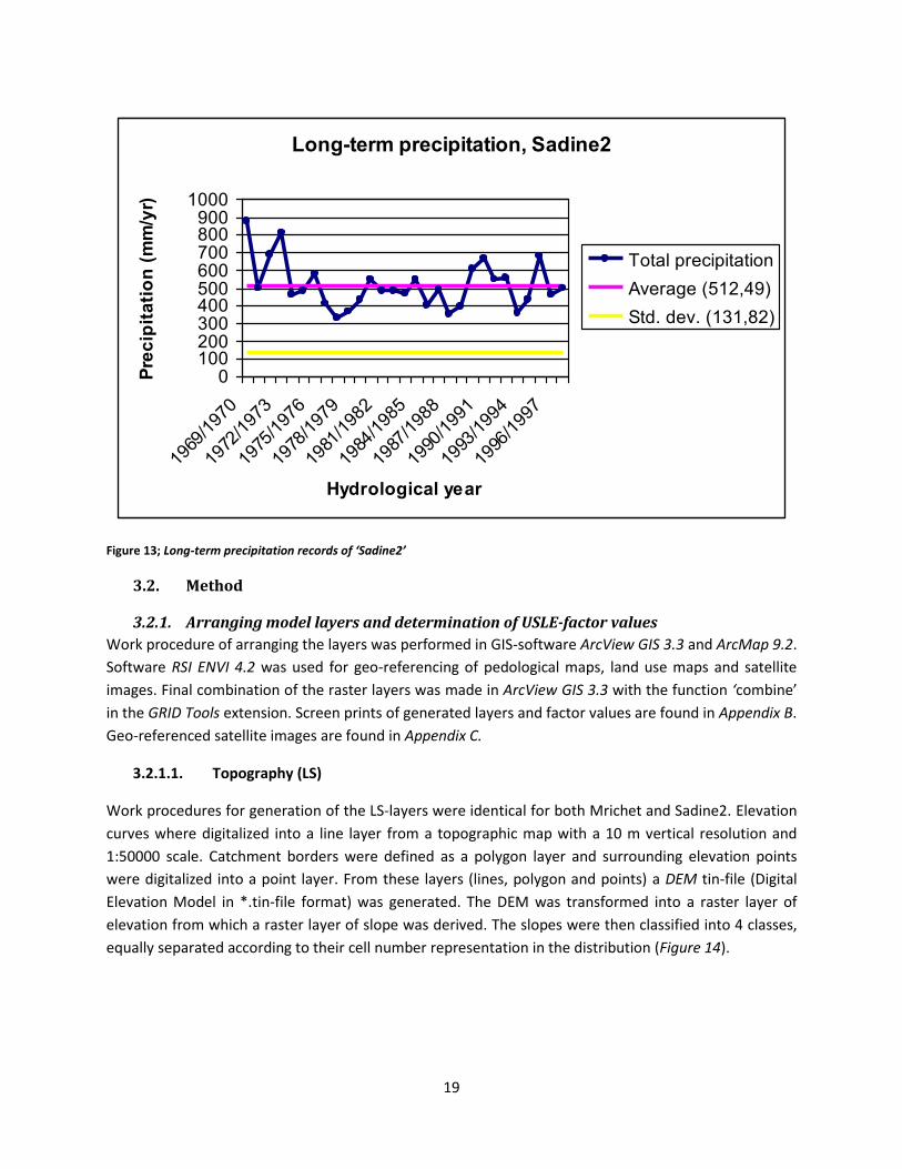
3.1.2. Sadine2

Sadine2 catchment (Figure 12) has an area of 6.53 km2 (653ha) of which 62% is agricultural land

(Convention CES/IRD, 1996-2002). Elevation ranges over 436 meters and the average slope is 17.0%

(Jebari et al, 2010). The reservoir of Sadine2 was constructed in 1990 and holds a total volume of

108 800 m3 of which 98.0 % (106 585 m3) was silted at the last measurement, 2000-07-12 (Convention

CES/IRD, 1996-2002). A detailed automatic precipitation recording device was installed 1994-02-28 and

records are available to 1998-09-16. The average precipitation (1969-1998) is about 512 mm/yr with a

standard deviation of 132 mm/yr (Figure 13). Observed average annual soil loss Aave is 24.5 ton ha-1 yr-1

(recorded 1991-1999) and the maximum annual soil loss Amax= 59.1 ton ha-1 yr-1 (recorded 1996-05-29 till

1998-03-17).

Long-term precipitation, Mrichet

0100200300400500600700800

1969

/197

0

1972

/197

3

1975

/197

6

1978

/197

9

1981

/198

2

1984

/198

5

1987

/198

8

1990

/199

1

1993

/199

4

1996

/199

7

Hydrological year

Pre

cip

itati

on

(m

m/y

r)

Total precipitation

Average (406,88)

Std. dev. (120,78)

18

Figure 12; The hydrological network of ‘Sadine2’

19

Figure 13; Long-term precipitation records of ‘Sadine2’

3.2. Method

3.2.1. Arranging model layers and determination of USLE-factor values

Work procedure of arranging the layers was performed in GIS-software ArcView GIS 3.3 and ArcMap 9.2.

Software RSI ENVI 4.2 was used for geo-referencing of pedological maps, land use maps and satellite

images. Final combination of the raster layers was made in ArcView GIS 3.3 with the function ‘combine’

in the GRID Tools extension. Screen prints of generated layers and factor values are found in Appendix B.

Geo-referenced satellite images are found in Appendix C.

3.2.1.1. Topography (LS)

Work procedures for generation of the LS-layers were identical for both Mrichet and Sadine2. Elevation

curves where digitalized into a line layer from a topographic map with a 10 m vertical resolution and

1:50000 scale. Catchment borders were defined as a polygon layer and surrounding elevation points

were digitalized into a point layer. From these layers (lines, polygon and points) a DEM tin-file (Digital

Elevation Model in *.tin-file format) was generated. The DEM was transformed into a raster layer of

elevation from which a raster layer of slope was derived. The slopes were then classified into 4 classes,

equally separated according to their cell number representation in the distribution (Figure 14).

Long-term precipitation, Sadine2

0100200300400500600700800900

1000

1969

/197

0

1972

/197

3

1975

/197

6

1978

/197

9

1981

/198

2

1984

/198

5

1987

/198

8

1990

/199

1

1993

/199

4

1996

/199

7

Hydrological year

Pre

cip

ita

tio

n (

mm

/yr)

Total precipitation

Average (512,49)

Std. dev. (131,82)

20

Figur 14; Example (Sadine2) of slope classification. All slopes were equally divided into four classes due to representation in

cell numbers. Number of cells are on the Y-axis, slope in % is on the X-axis.

Finally the LS-factor values for every class were calculated through the equation (eq.2) recommended by

Morgan and Davidson (1991). The slope steepness S used was the average value of every class. The

slope length L was difficult to estimate properly and therefore assigned the value of 22 m, the same

length as the original Whichmeier experimental plots (FAO, 1996).

3.2.1.2. Soil Erodibility (K)

For Mrichet, the K-factor layer was digitalized and divided into polygons from a pedological map

(Convention CES/IRD, 1998). The K-factor layer for Sadine2 was generated from a digital soil map (a GIS

polygon shape file) received from the ‘Tunisian Ministerè de L’agriculture et des Resources

Hydrologiques’ (2010). The K-factor values (Table 2) for both catchments were deduced from literature

(Zante et al, 2001; Dangler et al, 1976; Prog. D’actions Prioritaires, 1998) and consulting local experts.

21

Table 2; Theoretically determined K-factor values for the soil types represented in both catchments.

Soil type K-factor value

Vertisol 0.019

Brown, calcareous / vertic 0.020

Lithosol / regosol 0.021

Brown, calcareous 0.033

Raw mineral 0.036

Less developed / vertic 0.036

Lithosol / rendzina 0.050

Lithosol / brown calcareous 0.050

Complex 0.050

Less developed 0.054

Rendzina 0.100

Water body 0.000

3.2.1.3. Rainfall Erosivity (R)

In both sites the rainfall erosivity factor was considered constant over the entire catchment area. This is

a generalization due to lack of data, having only one rain gauge on each site. The R-factor value was

determined according to the Whichmeier method (OMM/WCP, 1983) (see Appendix A for calculations);

only taking storm events exceeding 12.7 mm into consideration and using the 30-min maximum

intensities I30. In comparison a second value was also calculated for 15-min intensities I15, as proposed by

Jebari (2009) for R-factor values in semiarid regions. The rainfall data used was given in 5-min intervals

of the event intensity. R-factor values were determined for two periods. The first was for the total time

period of available rainfall data using the complete hydrological years (1st September to the 31st August);

‘HY-period’. The second was for the period of maximum observed erosion; ‘Amax-period’ (see ‘Appendix

A’ for more details concerning R-factor determination).

Mrichet R-factor - data conditions and determination;

- Data was available from 1993-09-24 to 2002-09-25 and no data was missing within the period of

measurements. The period covers eight complete hydrological years from 1994/1995 to

2001/2002. The maximum observed Amax was observed from 1996-05-29 to 1998-03-17.

- The period had a total of 55 valid events of which 54 were within the eight hydrological years,

giving an average of 6.75 events / year for the HY-period.

- HY-period; R15 = 159,49 and R30 = 111,34 (ton ha-1 yr-1)

- Amax-period; R15 = 168.01 and R30 = 119.03 (ton ha-1 yr-1)

Sadine2 R-factor - data conditions and determination;

22

- Data was available from 1994-03-24 to 1998-09-16 and no data was missing in the period of

measurements. The period covers four complete hydrological years from 1994/1995 to

1997/1998. The maximum observed Amax was observed from 1994-06-14 to 1996-05-07.

- This period had 30 valid events of which all are within the four hydrological years, giving an

average of 7.5 events / year for the HY-period.

- HY-period; R15 = 115.82 and R30 = 85.47 (ton ha-1 yr-1)

- Amax-period; R15 = 71.17 and R30 = 62.84 (ton ha-1 yr-1)

Figure 15 shows the determined R-factor values for the different time periods.

3.2.1.4. Crop management factor (C)

For both catchments the C-factor layer was constructed from a land use map (Convention CES/IRD,

1998) digitally divided into polygons representing each land use class. Parts of this layer were then

revised or confirmed by in-field observations and by studying Google Earth satellite images. C-factor

values were determined from the report of Zante et al (2001). Missing values were taken from previous

studies (Jebari, 2009; Beskow et al, 2009; Jain et al, 2010; Erdogan et al, 2006) or assumed by

estimation. Table 3 displays the different land use classes used for Mrichet and Sadine2 with

corresponding C-factor values.

0

20

40

60

80

100

120

140

160

180

HY-per. Max. per.

R-f

acto

r valu

e (

ton

ha

-1 y

r-1)

Mrichet R15/R30 comparison

R15

R30

0

20

40

60

80

100

120

140

HY-per. Max per.

R-f

acto

r valu

e (

ton

ha

-1 y

r-1)

Sadine2 R15/R30 comparison

R15

R30

Figure 15; R-factor values of ‘Mrichet’ and ‘Sadine2'. In Mrichet, the R-factor is slightly higher for the Amax-period, for Sadine2

it is lower.

23

Table 3; The determined C-factor values for the catchments

Land use C-factor value

Water body 0.000

Forest, dense 0.015

Forest, light 0.100

Habitats 0.100

Roads 0.130

Tree plot, cherry 0.180

Scrubland 0.250

Crop-fallow rotation 0.500

Wedi 0.700

3.2.1.5. Conservation practice factor (P)

The P-factor layer was drawn as a polygon layer from geo-referenced satellite images (Google Earth,

2010), and then converted to raster layers.

The only observed conservation practices for Mrichet were some banquettes in the north east of the

catchment (Figure 16).

Figure 16; Banquettes in Mrichet

These banquettes are most likely to have a very low influence due to the small area they affect, but are

still taken into consideration for the P-factor. The area connected up-slope of each banquette was

24

assigned the value of 0.10. According to Zante et al (2001) this is the conservation practice value for

‘banquettes with or without plantations’ on 5-10% slopes.

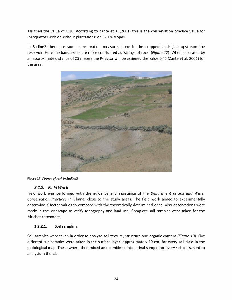
In Sadine2 there are some conservation measures done in the cropped lands just upstream the

reservoir. Here the banquettes are more considered as ‘strings of rock’ (Figure 17). When separated by

an approximate distance of 25 meters the P-factor will be assigned the value 0.45 (Zante et al, 2001) for

the area.

Figure 17; Strings of rock in Sadine2

3.2.2. Field Work

Field work was performed with the guidance and assistance of the Department of Soil and Water

Conservation Practices in Siliana, close to the study areas. The field work aimed to experimentally

determine K-factor values to compare with the theoretically determined ones. Also observations were

made in the landscape to verify topography and land use. Complete soil samples were taken for the

Mrichet catchment.

3.2.2.1. Soil sampling

Soil samples were taken in order to analyze soil texture, structure and organic content (Figure 18). Five

different sub-samples were taken in the surface layer (approximately 10 cm) for every soil class in the

pedological map. These where then mixed and combined into a final sample for every soil class, sent to

analysis in the lab.

25

Figure 18; Field soil sampling with local experts

3.2.2.2. Permeability - Infiltration Tests

The infiltration capacity of each soil class in both catchments was measured with a field test. Two pipes

were arranged on horizontal and non-cropped soil (Figure 19). The purpose of the outer pipe is to

maintain a constant downward infiltration flow surrounding the inner pipe. This will reduce the lateral

infiltration and direct the infiltrating water of the inner pipe downwards (Figure 19). A constant head of

30 mm is kept in the inner pipe while infiltrated amount of water (required refill to maintain the 30 mm

head) is noted in a specific time interval ranging over 60 minutes.

26

Figure 19; Infiltration tests in the field - the infiltrated water is measured over 60 minutes while keeping a constant head.

Lateral infiltration is reduced by using an additional outer ring with a constant head.

3.2.2.3. Soil aggregate structure tests

The durability in the aggregates of the soil types was also observed by placing a lumped sample in water

and study how it was affected. In most samples it was seen in a few minutes how the cohesive and

gravitational forces acted on the aggregate when soaked (Figure 20).

Figure 20; Soil aggregate test to study the durability of a soaked sample.

27

3.2.2.4. Field observations

The field visits also aim to confirm the reality of the catchments with how they are interpreted from

available data. Comparisons were done with reality and the generated topography (LS), land use (C) and

conservation practices (P) maps to confirm the conditions of the model as well as making corrections. In

Mrichet for example, an apple tree orchard in the map was missing, while a cherry tree plot not marked

on the map was found. Also in Sadine2 there were differences in observed reality and land use maps;

the land use map class ‘forest’ had a very low density of vegetation and was revised to ‘light forest’ due

to the field observations. Also two different definitions of the catchment border were found for Sadine2,

one by Convention CES/IRD (1998) and on by Convention CES/IRD (1996-2002). The definition to use

could be determined through field observations and further comparisons with the topographical map.

3.2.3. Calibration

After defining all input data the model was calibrated against observed soil loss values. The

methodology of the calibration was to compare estimated and observed soil loss and adjust the input

parameters to match the model with observed reality. The general methodology was to calibrate on the

Mrichet catchment since it had a less complex topography, and then confirm the settings by running the

same conditions for Sadine2.

3.2.3.1. K-, C-, and P-factor layers

The content of the K-, C- and P-factor layers were not really considered for calibration since it is more or

less defined by the available input data and cannot be changed without changing the definition of these.

USLE-factors considered in the calibration were thereby the R-factor and the LS-factor.

3.2.3.2. R-factor

As mentioned, the R-factor is considered constant for the entire catchment and is represented by a

single value. As seen in Figure 21 it does not seem to be any correlation between the calculated R-factor

values for the two periods considered and the different observed soil losses for the same periods; in

Mrichet the R is only slightly increased and for Sadine2 it is actually decreased for the ‘Amax-period’.

Based on the recommendations in the Whichmeier approach to use long term data, preferably 20 years

(FAO, 1996), and the non-existing correlation to the ‘Amax-period’, the R-factors were determined from

the ‘HY-period’ was used for the calibration. It was also found that the soil loss was more accurately

estimated with R15 as proposed by Jebari (2009), why this value was used.

28

3.2.3.3. LS-factor layer

Topographic factor LS is represented by a more complex layer. The slope steepness is very much

affected by how you chose the grid cell dimensions in the DEM. Wu et al (2005) states that the

estimation of soil loss by empirical models decreases significantly when the grid cell size is increased.

This is mainly due to the reduction in general slope steepness. The next step in the calibration was

therefore mainly focused on determining the right conditions for the LS-factor layer in terms of the grid

cell resolution. In order to calibrate the model it was executed using a 10, 15, 20, 25, 30, 40 and 50

meter grid cell size.

3.2.3.4. The Grid Cell Dimension

Also when combining raster layers in an overlay operation it is necessary to use uniform cell dimensions

and distribution for all layers (Larsson & Harrie, 2005). In case of differences in cell dimensions it is

possible that the software will distort the values due to a generalization in the operation algorithm

(Larsson, 2010). In order to overcome this issue, all layers are generated with the same grid cell

resolution as the LS-factor layer throughout the calibration.

3.2.3.5. Calibration Summary

- K-, C- and P-factor layers are not considered for calibration

- The R-factor value best suited is R15

- The LS-factor layers were generated for 10, 15, 20, 25, 30, 40 and 50 meter grid cell sizes.

- All layers were generated in the same grid cell sizes as the LS-factor layer.

Sadine2 - R-factor values and

observed annual soil loss

0

20

40

60

80

100

120

140

HY-per. Max per.

R-f

acto

r valu

e

0

10

20

30

40

50

60

70

Ob

s.

an

nu

al

so

il l

oss A

(to

n/h

a/y

r)

R15

R30

A

Mrichet - R-factor values and

observed annual soil loss

0

20

40

60

80

100

120

140

160

180

HY-per. Max. per.

R-f

acto

r valu

e

0

5

10

15

20

25

Ob

s.

an

nu

al

so

il l

oss A

(to

n/h

a/y

r) R15

R30

A

Figure 21; Comparison of soil loss (A) and R-factor values (R15 and R30) for the HY-period and the Amax-period.

29

4. Results

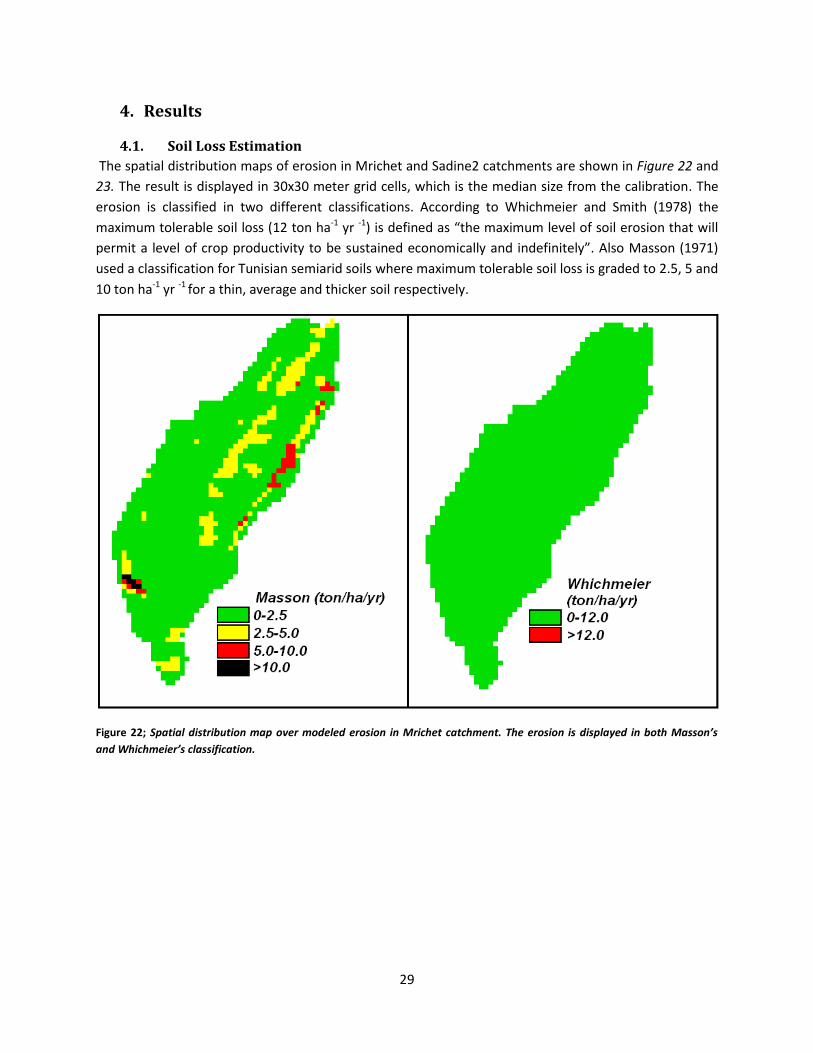
4.1. Soil Loss Estimation

The spatial distribution maps of erosion in Mrichet and Sadine2 catchments are shown in Figure 22 and

23. The result is displayed in 30x30 meter grid cells, which is the median size from the calibration. The

erosion is classified in two different classifications. According to Whichmeier and Smith (1978) the

maximum tolerable soil loss (12 ton ha-1 yr -1) is defined as “the maximum level of soil erosion that will

permit a level of crop productivity to be sustained economically and indefinitely”. Also Masson (1971)

used a classification for Tunisian semiarid soils where maximum tolerable soil loss is graded to 2.5, 5 and

10 ton ha-1 yr -1 for a thin, average and thicker soil respectively.

Figure 22; Spatial distribution map over modeled erosion in Mrichet catchment. The erosion is displayed in both Masson’s

and Whichmeier’s classification.

30

Figure 23; Spatial distribution map over modeled erosion in Sadine2 catchment. The erosion is displayed in both Masson’s

and Whichmeier’s classification.

Figure 24 (Mrichet) and 25 (Sadine2) shows the simulation results in terms of catchment average annual

soil loss, plotted against the different grid cell sizes used in the calibration. The comparative observed

erosion is for Mrichet 11.4 ton ha-1 yr -1 and for Sadine2 24.5 ton ha-1 yr -1. The modeled soil loss is very

much too low in comparison with observed siltation records. However, if comparing the deviation from

the observed data it is seen that the errors are in the same order of magnitude in both catchments

(Figure 26).

31

Figure 24; Calibration results for Mrichet catchment, the comparative observed erosion is 11.4 ton ha-1

yr-1

.

Figure 25; Calibration results for Sadine2 catchment, the comparative observed erosion is 24.5 ton ha-1

yr-1

1,3

1,4

1,5

1,6

1,7

1,8

1,9

0 10 20 30 40 50 60

Mrichet - simulated erosion and grid cell sizeE

(to

n/h

a/yr

)

Grid cell size (m)

2,8

2,9

3

3,1

3,2

3,3

3,4

3,5

3,6

3,7

3,8

0 10 20 30 40 50 60

Sadine2 - simulated erosion and grid cell size

E (t

on

/ha/

yr)

Grid cell size (m)

32

Figure 26; The errors of both catchments are in the same order of magnitude

4.2. Field Work

The determination of comparative K-factor values was performed according to the USLE-principle in

chapter ‘2.3.1.2. Soil Erodibility Factor (K)’. Table 4 shows the lab analysis data used to determine

experimental K-factor values. Figure 27 shows the comparison with the theoretical values used in the

model.

Table 4; Determination of experimental K-factor values were ‘Fine sand + silt’ is grain sizes 0.002-0.100 mm, ‘Sand’ is 0.100 –

2 mm, ‘O.M.C.’ is organic matter content, ‘S.C.’ is structure class, ‘P.C.’ is permeability class, ‘K.us’ is K-factor value in US-units

and K.si is K-factor value in SI-units.

Soil

Fine sand

+ silt (%) Sand (%) O.M.C. (%)

S.C.

(1-4)

P.C.

(1-6) K.us Ksi

1. Less dev. / vertic 69,75 10,25 1,0 2 2 0,42 0,055

2. Lithosol / regosol 59,5 10,25 1,0 2 1 0,29 0,038

3. Rendzina 56,5 18,5 1,5 1 n/a n/a n/a

4. Lithosol / rendz. 66,75 8,25 1,0 2 1 0,35 0,046

5. Lithosol / brown calc. 56,75 13,25 0,9 2 1 0,26 0,034

6. Brown, calc. / vertic 49,5 13,5 1,3 3 2 0,24 0,032

7. Brown, calcareous 47 17,75 1,3 3 3 0,27 0,036

10

11

12

13

14

15

16

17

18

19

20

0 10 20 30 40 50

Mrichet

Sadine2

% o

f co

mp

arat

ive

ob

serv

ed s

oil

loss

val

ue

Grid cell size (m)

Comparison of the error of the catchments

33

Figure 27; Comparison of experimental and theoretical K-factor values in Mrichet catchment.

0

0,01

0,02

0,03

0,04

0,05

0,06

0,07

0,08

0,09

0,1

0,11

1 2 3 4 5 6 7

Experimental values

Theoretical values

K-f

acto

r va

lue

Soil classes; 1 = less dev./vertic, 2 = lithosol / regosol, 3 = Rendzina, 4 = Lithosol /rendzina,5 = Lithosol / brown calc., 6 = Brown calc. /vertic, 7 = Brown calcareous

Comparison of experimental and theoretical K-factor values

34

5. Discussion

5.1. Sources of Error –Generalizations, Approximations and Model Limitations

All working steps in creating the thematic layers of the model contain approximations and

generalizations of data to some extent. When topographic maps and satellite images are digitalized it is

hard to achieve exact precision due to low resolutions, low scales and deviations in the projection. As for

the satellite images the only available data was Google Earth, which is limited in resolution and also

turned out to be hard to geo-reference with high precision. However it was still useful in some

operations like definition of areas affected by conservation practices.

An example of a major generalization is displayed in the C-factor for both catchments; all agricultural

land was classified as crop-fallow rotation and assigned an average value for the entire class. Thus, this

generalization is necessary since the model is for long term conditions and the distribution of cropped

and fallow land changes on an annual basis.

In the original Whichmeier approach it is stated that the rainfall data record should be from a 20 years

period minimum. In this case, data was only available over eight (Mrichet) and four (Sadine2) years

respectively. The requirements of data are in general very low in this approach; however it would of

course be desirable to fulfill the requirements as they are defined in the original approach.

The main tool in the calibration was the grid cell size, affecting the LS-factor layer mainly. Every new grid

cell dimension required a new interpolation of the DEM into a raster layer of slope. This interpolation is

very much of a great importance of the model outcome. Obviously the LS-factor values then are very

dependent on the algorithm making this interpolation, why it could be of great interest to go deeper

into the software routine of this operation. In addition to the generalizations of the slope raster layer

generation there was also the slope length estimation. It was not possible to determine every single

slope length so a fixed value was used. To neutralize the influence of the slope length, which was

unknown for all slopes, the original 22m length was assumed (the length Whichmeier used in his original

experimental plots when empirically developing the USLE).

Apart from the work on the grid cell size and the LS-factor a sensitivity analysis was performed on the

other parameters. By changing parameter values one at the time it was possible to see how the

estimated erosion was affected. However, the model equation is a simple multiplication of the

parameters, why the sensitivity of every parameter is linear – a duplication of any parameter value

would directly lead to a duplication of the estimated soil erosion.

The limitations of the USLE are mentioned in the literature review (chapter 2.3.2. Limitations) and it is

clearly stated that the model only estimates rill and inter-rill erosion. This means that no wind erosion is

taken in consideration for the simulation. However this kind of erosion is not necessarily deposited in

the reservoir in which the comparative values used in the calibration are estimated. Therefore wind

erosion contribution is probably not included in the observed comparative values.

One of the main limitations of the USLE/GIS concept could be the absence of mass-, channel- and gully

erosion in the simulation. The estimated erosion is very much too low and this may very well be because

35

of the exclusion of mass-, channel and gully erosion in the model. As seen in Figure 28, mass erosion is

acting on the catchments. The comparative values observed as siltation in the catchment reservoir

therefore probably originate from other kinds of water erosion in addition to the contribution from rill

and inter-rill erosion.

Figure 28; Not taking mass erosion in consideration is possibly one of the factors that causes the model to give unsatisfying

results.

5.2. Conclusion

The methodology as used in this approach does not seem to be applicable for semi-arid conditions. The

result of simulated erosion is very much too low in comparison with the observed records of siltation,

reaching only approximately 12-16 % of the observed values, depending on which grid cell size is used.

There may be several reasons why, but as discussed in chapter ‘3.2.3. Calibration’ it is hard to change

the values of C-, P- and K- factors without redefining them. However the K-factor values are possibly

underestimated for these regions; the USLE is originally not developed and defined under semi-arid

conditions.

Also the R-factor seem to be underestimated; in other studies the R-factor is often several or even up to

fifty times as high (Jain et al. 2010, Beskow et al. 2009) - however it is important to remember that the

precipitation is also more intense in these regions.

36

The method could possibly be improved by redefining the K- and R-factor determination for semi-arid

conditions. If adaptation to semi-arid conditions could be done, the USLE/GIS-approach can be a very

powerful and available tool when predicting soil loss. In general the approach is very much available

since restrictions in data easily can be overcome by approximations. Also the input data does not

require a very high level of details, which makes it very applicable when data is insufficient. An idea

could also be to determine the proportion of the comparative observed values that are represented by

rill and inter-rill erosion and thereby have a more accurate and realistic comparative value for the

calibration.

37

References

Literature and Articles

Beskow S., C. R. Mello, L. D. Norton, N., Curi, M.R. Viola, J.C. Avanzi, Soil erosion prediction in the Grande

River Basin, Brazil using distributed modelling, National Soil Erosion Research Laboratory, Purdue

University, USA, 2009.

Convention CES/IRD, Albergel, J., Pépin, Y., Boufaroua, M., et al, Annuaire Hydrologique des lacs

Collinaires 1994-1995 … 2000-2001, Direction de la Conservation Des Eaux et des Sols and Institut de

Recherche pour le développement, Tunisia, 1996-2002.

Dangler E. W., El-Swaify S. A., Ahuja L. R., Barnett A. P., Erodibility of selected Hawaii soils by rainfall

simulation, Agricultural research service, US department of agriculture, western region, 113 p., 1976

Erdogan H. E., Erpul G., Bayramin I.: Use of USLE/GIS Methodology for Predicting Soil Loss in a Semiarid

Agricultural Watershed, Department of Soil SIence, University of Ankara, Turkey, 2006

Fistikogli, O., Harmancioglu, N. B.: Integration of GIS with USLE in Assessment of Soil Erosion, Faculty of

Engineering, Dokuz Eylul University, Izmir, Turkey, 2002

Jain Manoj K., Mishra Surendra K., R B Shah: Estimation of sediment yield and areas vulnerable to soil

erosion and deposition in a Himalayan watershed using GIS, Dep. Of Hydrology, Indian Institute of

Technology, India, 2010

Jankauskas, B., Jankauskiene, G., Fullen, M. A., Relations between soil organic matter content and soil

erosion severity in Albeluvisols of the Žemaičiai Uplands, Kaltinenai Research Station of the Lithuanian

Institute of Agriculture, Lithuania, 2007.

Jebari, S., Berndtsson, R., Bahri, A., Boufaroua, M.: Exceptional Rainfall Characteristics Related to Erosion

Risk in Semiarid Tunisia, National Research Institute for Rural Engineering, Waters and Forestry, Ariana,

Tunis, Tunisia, 2008.

Jebari, S.: Water erosion modeling using fractal rainfall disaggregation – A study in semiarid Tunisia,

Water resources engineering, Lund University, Sweden, 2009.

Jebari, S., Berndtsson, R., Bahri, A., Boufaroua, M.: Spatial soil loss risk and reservoir siltation in semi-

arid Tunisia, Hydrological Siences Journal, 55:1, 121-137, 2010.

Larsson, K., Harrie, L., Introduktion till GIS – Geografiska Informationssystem, Institutionen för

naturgeografi och ekosystemanalys & GIS-centrum, Lunds Universitet, Lund, Sweden, 2005.

Masson, J.M.: Lérosion des sols par l’eau en climat Méditerranéen. Méthodes expérimentales pour

l’étude des quantities érodées a l’échelle du champ Thése de Docteur-Ingénieur, USTL Montpellier, 1971

38

Moore, I. and Burch, G., Physical basis of the length-slope factor in the universal soil loss equation. Soil

Sci. Soc. Am. J., 1986a.

Moore, I. and Burch, G., Modeling erosion and deposition: topographic effects. Trans ASAE, 1986b

Moore, I. and Wilson, J. P., Length slope factor for the revised universal soil loss equation: simplified

method of solution. J. Soil Water Conserv., 1992

Morgan, R.P.C., Davidson D. A.: Soil Erosion and Conservation, Longman Group, U.K, 1991.

OMM/WCP/M. C. Babau, La pluie et son agressivite en tant que facteur de l’erosion, Organisation

Metrologique Mondiale / World Climate Programme, 1983.

Onyando J. O., Kisoyan P., Chemelil M. C.: Estimation of Potential Soil Erosion for River Perkerra

Catchment in Kenya, Department of Agricultural Engineering, Egerton University, Njoro Kenya, 2004

Programme D’actions prioritaires, DIRECTIVES pour la cartographie et la mesure des processus d’érosion

hydrique dans les zones côtières méditerranéennes, Programme D’actions prioritaires, Croatia, 1998

Strahler A., Strahler A.: Introducing Physical Geography, 3rd edition, John Wiley & Sons inc., USA, 2003.

Toy, J. T., Foster, R. G, Renard, K. G.: Soil Erosion – Processes, Prediction, Measurement and Control,

John Wiley & Sons inc., USA, 2002.

Zante P., Collinet J., Leclerc G.: Cartographie des risques érosifs sur le basin versant de la retenue

collinaire d’Abdessadok (nord dorsale tunisienne), Institut de Recherche pour dèveloppement, Tunisia,

2001

Ward R. C., Robinson M.: Principles of Hydrology, 4th edition, McGraw-Hill Publishing Company, England,

2000.

Whichmeier, W.H., and Smith, D.D: Predicting rainfall erosion losses – A guide to conservation planning.

USDA Agriculture Handbook 537, Washington DC: GPO 1978

Wu, S.; Li, J., Huang, G.: An evaluation of grid size uncertainty in empirical soil loss modeling with digital

elevation models, Department of Agriculture, Regina, Saskatchewan, Canada, 2005.

Online

FAO 1990: The conservation and rehabilitation of African lands -an international scheme, Food and

Agriculture Organization of the United Nations, 1990. [online] accessed 2010-02-10

http://www.fao.org/docrep/z5700e/z5700e00.htm#Contents

FAO 1996: Land husbandry - Components and strategy, Food and Agriculture Organization of the United

Nations, 1996. [online] accessed 2010-03-11

http://www.fao.org/docrep/t1765e/t1765e00.htm#Contents

39

Ministerè de l’agriculture et des resources hydrologiques, Tunisia, [online] accessed 2010-04-13

http://www.carteagricole.agrinet.tn/WEB/Produits/MCD/dd.htm#_Toc9840552

Stone & Hilborn, 2000: FACTSHEET, Universal Soil Loss Equation, Ministry of Agriculture, Food and Rural

Affairs, 2000, [online] accessed 2010-03-11

http://www.omafra.gov.on.ca/english/engineer/facts/00-001.htm#background

USDA/NSERL: USLE Database, United States Department of Agriculture /National Soil Erosion Research

Laboratory, [online] accessed 2010-03-11

http://topsoil.nserl.purdue.edu/usle/page7.html

Figures

Columbia University, 2008: Hjulström diagram, [online] accessed 2010-03-12

http://eesc.columbia.edu/courses/ees/lithosphere/homework/hmwk2.gif

Convention CES/IRD, Direction de la Conservation Des Eaux et des Sols and Institut de Recherche pour le

développement, Tunisia 1998

FAO, 1996b, K-factor determination, [online] accessed 2010-05-20

http://www.fao.org/docrep/t1765e/t1765e0f.htm#soil erodibility

Fistikogli, O., Harmancioglu, N. B.: Integration of GIS with USLE in Assessment of Soil Erosion, Faculty of

Engineering, Dokuz Eylul University, Izmir, Turkey, 2002

Jebari, S.: personal e-mail communication, 2009.

Larsson, K. and Harrie, L., Introduktion till GIS – Geografiska Informationssystem, Institutionen för

naturgeografi och ekosystemanalys & GIS-centrum, Lunds Universitet, Lund, Sweden, 2005.

Other

Larsson, K.: Information from email correspondence concerning overlay operations of GIS-raster layers

with different grid cell resolutions, Institutionen för naturgeografi och ekosystemanalys & GIS-centrum,

Lunds Universitet, Lund, Sweden., 2010-05-06.

40

Appendix A – R-factor R-factor calculation; example

The R-factor was determined according to the original Wischmeier approach as described by OMM/WCP

(1983). The example displayed here is the determination of R30 for an event recorded in the Mrichet

catchment, dated to 28 Mars 1999. The event depth is 20 mm and duration is 5 h 15 min.

Table A1 shows the values of the calculation and the procedure is explained in the steps below.

Table A1; Calculation example for determination of R-factor.

i time Pac (mm) Ps (30min) Is (mm/h) Imax (mm/h) e E Etot R

1 14:30 0 0 0 9 - - 362,684 4,765191

2 15:00 2,5 2,5 5 18,00201 45,00502

3 15:30 5 2,5 5 18,00201 45,00502

4 16:00 9,5 4,5 9 20,23054 91,03742

5 16:30 12,5 3 6 18,69326 56,07978

6 17:00 15,5 3 6 18,69326 56,07978

7 17:30 17,25 1,75 3,5 16,64971 29,137

8 18:00 19,167 1,917 3,834 16,99528 32,57996

9 18:30 19,605 0,438 0,876 11,39806 4,992351

10 19:00 19,763 0,158 0,316 7,532268 1,190098

11 19:30 19,921 0,158 0,316 7,532268 1,190098

12 19:45 20 0,079 0,158 4,904276 0,387438

Calculation procedure;

- Pac is accumulated rainfall depth, recorded in field

- Ps is the rainfall depth of each 30-min segment (Pac, i - Pac, i-1)

- Is is the rainfall intensity of each 30-min segment (Ps ∙ 2)

- Imax is the maximum intensity determined from column Is

- e is the kinetic energy / mm of each 30-min segment, determined by eq. X1

- E is the kinetic energy of every 30-min segment (ei ∙ Ps, i)

- Etot is the sum of E for the entire event

- R is the event R-factor determined by eq. X2

41

Note that the last segment i=13 is insufficient in time period. The segment intensity Is is still calculated

by multiplication by two, as proposed for events with duration less than 30 minutes (OMM/WCP, 1983).

The total annual R-factor is then equal to the sum of all events within the year and finally annual

averages are determined.

9,11log73,8 sIe eq. X1

685

maxIER tot eq. X2

Valid events and determined R-factors

Table A2 shows the 55 valid rainfall events of Mrichet catchment in the period 1993-09-24 to 2002-09-

25 (P = mm, duration = hh:mm, I = mm/h);

Table A2; The valid rainfall events of Mrichet

Year Month Day Nr P Duration I15 I30 R15 R30 Hydr. Yr R15 R30

1994 Jan 8 1 18 02:55 12 10 5,968684644 4,953939

Sep 9 2 18 01:30 76 65 217,3408274 185,1979

Sep 27 3 73 07:25 20 16 9,671233938 7,660493

Oct 3 4 28,5 04:05 58 38 57,59423271 37,01169

1995 Mar 12 5 14 06:00 6 6 7,846365354 3,906067 1994/1995 292,5 233,8

Sep 20 6 16,5 00:35 40 20 94,81395527 21,78923

Sep 22 7 14,5 01:00 47,33 25,67 99,08499426 25,33283

Sep 24 8 16 00:20 50 32 119,9474581 37,432

Nov 2 9 24,5 03:10 24 14 69,7924028 19,76258

1996 Jan 11 10 24 10:25 10 7,33 5,590560246 4,071428

Jan 13 11 27,5 10:35 6 6 3,862971091 3,832277

Feb 7 12 15 06:00 7 4,5 2,407591845 1,520114

Feb 8 13 20,5 06:40 8 8 4,022177024 3,938873

Feb 27 14 23,5 09:10 6 4,67 3,209964139 2,458159

Feb 27 15 16 11:20 4 3,17 1,261929825 0,988085

42

Mar 14 16 19,5 04:05 12 11,5 6,237775813 5,890872

Apr 29 17 13 04:00 10 9 3,343824947 3,002113

May 10 18 52,5 03:05 58 36 109,3898416 66,44242

Aug 14 19 16 00:55 38 21 21,19453004 11,00227 1995/1996 544,2 207,5

Sep 9 20 33,5 03:00 56 38,5 65,12305478 44,01919

Sep 16 21 24,5 01:15 44 38 38,28943198 32,63285

1997 Jan 25 22 13 05:40 6 5 1,811550875 1,483335

Apr 9 23 41,5 16:25 6 6 5,992459941 5,97816

Jun 1 24 28,5 01:10 48 28,5 50,04636928 27,87528 1996/1997 161,3 112

Sep 6 25 13 01:45 22 12,5 8,605089183 4,690256

Oct 5 26 50,5 02:25 42 35 74,37523252 61,50293

Oct 13 27 14,5 00:55 34 20 16,91576344 9,448681

Nov 12 28 16 04:55 8 6 3,254890914 2,375777

Nov 23 29 26,5 06:20 14 11 10,32224852 8,077637

Dec 23 30 20 08:30 7 6 3,264808034 2,787771

1998 Feb 27 31 13,5 06:10 10 7,5 3,222270539 2,382566

Jun 6 32 18 01:20 37 31,17 23,08370213 19,35898 1997/1998 143 110,6

Sep 23 33 52,5 05:25 26 17 42,43581205 27,44091

Oct 10 34 16,5 06:00 8 5,5 3,164036719 2,153025

Nov 28 35 13 06:25 6,4 4 1,836364805 1,125255

1999 Jan 17 36 16 09:30 5,33 3,83 1,887319865 1,325646

Jan 19 37 56 18:05 10 7 14,02840351 9,714972

Mar 28 38 20 05:05 12 9 6,423106801 4,765191

May 8 39 15 04:05 10 8 3,945457521 3,119766

Jun 4 40 19,5 00:20 74 39 58,24893824 28,63254 1998/1999 132 78,28

Sep 9 41 23 02:00 30 18 22,64438295 13,06464

43

Nov 27 42 55,5 14:15 16 10,5 23,62485923 15,35133

Nov 28 43 16 02:30 16 12,33 7,784804383 5,897444 1999/2000 54,05 34,31

2000 Sep 12 44 22 01:45 34 28 25,1137981 20,29682

Sep 12 45 32,5 02:20 34 19,33 37,18074812 20,46022

Sep 27 46 17,5 01:35 48 30 29,44484585 17,88713

Sep 28 47 15,5 02:30 19,6 11 8,824887624 4,782631

Okt 20 48 15,5 03:55 18 11 7,621159189 4,52708

Okt 21 49 5,5 06:45 22 12,25 20,8373352 11,08866

2001 May 4 50 25,5 07:00 8 7 5,226950783 4,536584

May 11 51 26,5 10:55 10 9 6,423536953 5,753429 2000/2001 140,7 89,33

Sep 29 52 27 00:40 58 50 60,03945188 51,28556

2002 Mar 17 53 17 02:45 30 21 15,87114392 10,89728

Mar 17 54 29 04:05 12 9 10,00770398 7,419273

May 7 55 14,5 00:35 32 20 16,01172583 9,448681 2001/2002 101,9 79,05

Table A3 shows the 30 valid rainfall events of Sadine2 catchment in the period 1994-03-24 to 1998-09-

16 (P = mm, duration = hh:mm, I = mm/h);

Table A3; The valid rainfall events of Sadine2

Year Month Day Nr P Duration I15 I30 R15 R30 Hydr. Yr R15 R30

1994 Apr 16 1 20 03:20 16 13,29 9,3093 7,6855

Jul 31 2 38 00:40 66 64 99,157 94,673

1995 Jun 24 3 13,5 01:40 26 20,27 11,19 8,5369 1994/1995 110,3466 103,2104

Oct 15 4 23 05:05 20 12 12,918 7,5852

1996 Jan 30 5 15,5 08:15 5 4,5 1,7028 1,5251

Feb 7 6 17 09:20 6 3 2,1925 1,0864

44

Feb 8 7 20 06:00 10 6 5,0211 2,9692

Apr 29 8 15 05:20 8 8 3,0329 3,0139

May 10 9 18,5 03:30 36 24 21,614 13,99

Aug 8 10 16 00:15 50 32 29,987 18,716

Aug 15 11 25 00:45 44 35 40,617 31,188

Aug 17 12 13,5 00:20 32 27 15,427 12,981 1995/1996 132,511 93,05585

Sep 9 13 24 00:55 42 25 36,723 20,98

1997 Jan 11 14 64,5 22:10 10 7 15,713 10,916

Jan 12 15 20,5 12:10 6 4,67 2,6277 2,0194

Jan 26 16 19,5 07:45 6 5,5 2,8524 2,5818

Mar 15 17 14 09:45 8 5,4 2,4425 1,6131

Apr 24 18 14 03:30 8 8 2,9226 2,9031

May 17 19 17 00:40 44 33 27,357 20,283

Aug 5 20 15 00:55 42 23 22,05 11,451 1996/1997 112,6879 72,74749

Sep 21 21 21 00:40 54 38 42,12 28,983

Nov 23 22 24 05:05 10 8 6,5543 5,2084

Dec 6 23 21 07:45 6 6 3,0512 3,0325

Dec 23 24 13,5 08:40 7 5 2,0354 1,4356

1998 Feb 27 25 21,5 06:05 8 7 4,4003 3,8215

Mar 15 26 34 10:45 12 8 10,336 6,8062

Mar 30 27 14,5 04:25 12 10 4,6675 3,8411

Apr 22 28 13,5 05:30 5 4 1,5541 1,2315

May 16 29 13 03:25 13 10 4,5476 3,4678

Jun 6 30 15,5 00:45 50 28 28,484 15,025 1997/1998 107,7505 72,852

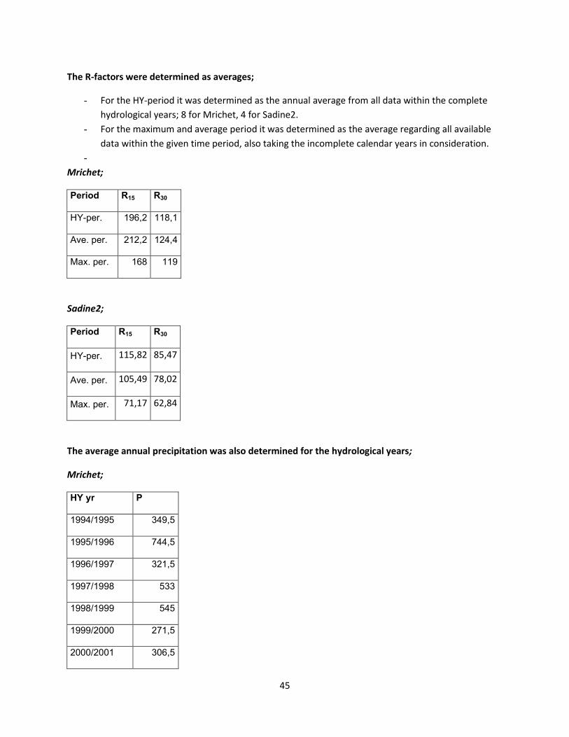
45

The R-factors were determined as averages;

- For the HY-period it was determined as the annual average from all data within the complete

hydrological years; 8 for Mrichet, 4 for Sadine2.

- For the maximum and average period it was determined as the average regarding all available

data within the given time period, also taking the incomplete calendar years in consideration.

-

Mrichet;

Period R15 R30

HY-per. 196,2 118,1

Ave. per. 212,2 124,4

Max. per. 168 119

Sadine2;

Period R15 R30

HY-per. 115,82 85,47

Ave. per. 105,49 78,02

Max. per. 71,17 62,84

The average annual precipitation was also determined for the hydrological years;

Mrichet;

HY yr P

1994/1995 349,5

1995/1996 744,5

1996/1997 321,5

1997/1998 533

1998/1999 545

1999/2000 271,5

2000/2001 306,5

46

2001/2002 307,5

Average; 422,375

Sadine2;

HY yr P

1994/1995 242

1995/1996 589

1996/1997 426,5

1997/1998 501,5

Average; 439,75

47

Appendix B – Thematic layers Mrichet – C-factor - Land use

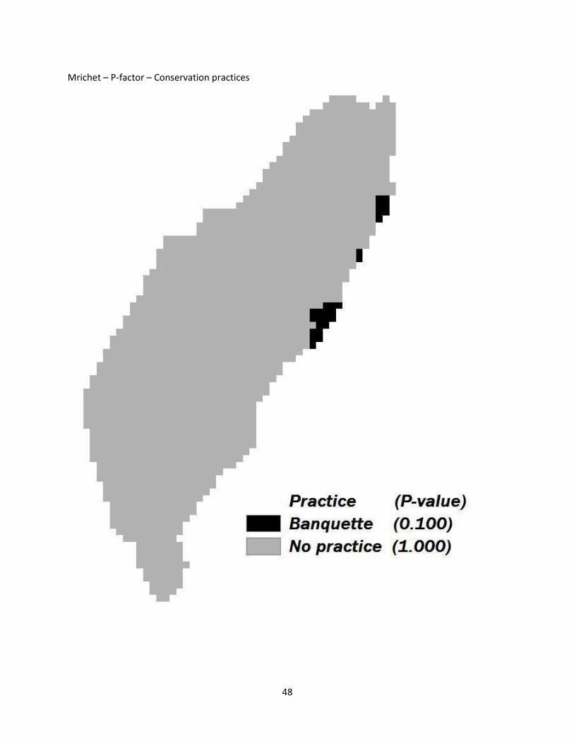
48

Mrichet – P-factor – Conservation practices

49

Mrichet – K-factor – Pedology

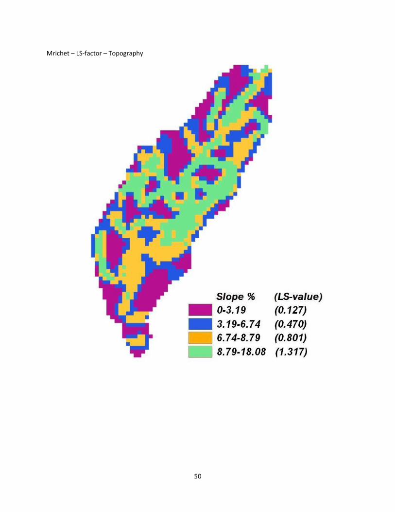
50

Mrichet – LS-factor – Topography

51

Sadine2 – C-factor - Land use

52

Sadine2 – P-factor – Conservation Practices

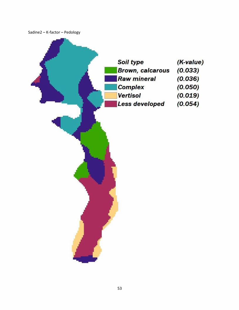
53

Sadine2 – K-factor – Pedology

54

Sadine2 – LS-factor – Topography

55

Appendix C – Satellite Images Mrichet

56

Sadine2