software product* $70,000 bank loan $50,000 computers ...zz1802/finance...
TRANSCRIPT

1
Answers to Selected Problems
Chapter 1
1. (1.9)
a. The bank loan is a financial liability for Lanni. Lanni's IOU is the bank's financial
asset. The cash Lanni receives is a financial asset. The new financial asset created is
Lanni's promissory note held by the bank.
b. The cash paid by Lanni is the transfer of a financial asset to the software developer. In
return, Lanni gets a real asset, the completed software. No financial assets are created
or destroyed. Cash is simply transferred from one firm to another.
c. Lanni sells the software, which is a real asset, to Microsoft. In exchange Lanni
receives a financial asset, 5,000 shares of Microsoft stock. If Microsoft issues new
shares in order to pay Lanni, this would constitute the creation of new financial asset.
d. In selling 5,000 shares of stock for $125,000, Lanni is exchanging one financial asset
for another. In paying off the IOU with $50,000, Lanni is exchanging financial assets.
The loan is "destroyed" in the transaction, since it is retired when paid.
2. (1.10)
a.
Cash $70,000 Bank loan $50,000
Computers 30,000 Shareholders’ equity 50,000
Total $100,000 Total $100,000
Assets
Liabilities &
Shareholders’ Equity
Ratio of real to total assets = 000,100$
000,30$ = 0.3
b.
Software product* $70,000 Bank loan $50,000
Computers 30,000 Shareholders’ equity 50,000
Total $100,000 Total $100,000
*Value at cost
Assets
Liabilities &
Shareholders’ Equity
Ratio of real to total assets = 000,100$
000,100$ = 1.0
2
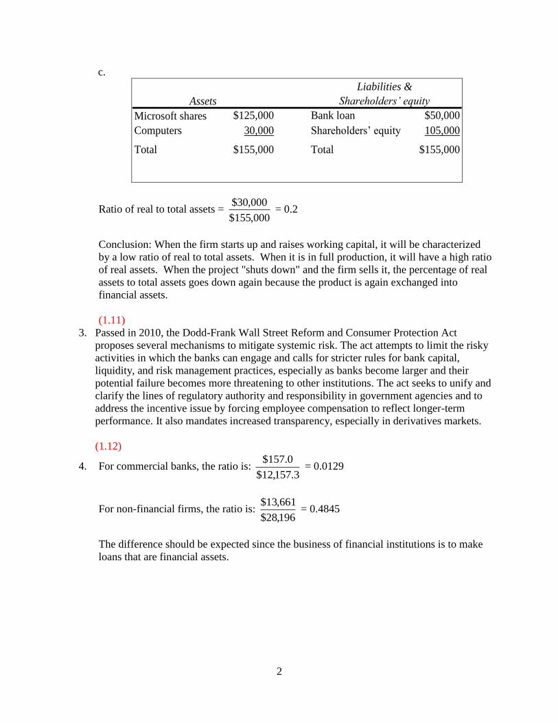
c.
Microsoft shares $125,000 Bank loan $50,000
Computers 30,000 Shareholders’ equity 105,000
Total $155,000 Total $155,000
Assets
Liabilities &
Shareholders’ equity
Ratio of real to total assets = 000,155$
000,30$ = 0.2
Conclusion: When the firm starts up and raises working capital, it will be characterized
by a low ratio of real to total assets. When it is in full production, it will have a high ratio
of real assets. When the project "shuts down" and the firm sells it, the percentage of real
assets to total assets goes down again because the product is again exchanged into
financial assets.
(1.11)
3. Passed in 2010, the Dodd-Frank Wall Street Reform and Consumer Protection Act
proposes several mechanisms to mitigate systemic risk. The act attempts to limit the risky
activities in which the banks can engage and calls for stricter rules for bank capital,
liquidity, and risk management practices, especially as banks become larger and their
potential failure becomes more threatening to other institutions. The act seeks to unify and
clarify the lines of regulatory authority and responsibility in government agencies and to
address the incentive issue by forcing employee compensation to reflect longer-term
performance. It also mandates increased transparency, especially in derivatives markets.
(1.12)
4. For commercial banks, the ratio is: 3.157,12$
0.157$ = 0.0129
For non-financial firms, the ratio is: 196,28$
661,13$ = 0.4845
The difference should be expected since the business of financial institutions is to make
loans that are financial assets.

3
(1.13)
5. National wealth is a measurement of the real assets used to produce GDP in the economy.
Financial assets are claims on those assets held by individuals.
Financial assets owned by households represent their claims on the real assets of the
issuers, and thus show up as wealth to households. Their interests in the issuers, on the
other hand, are obligations to the issuers. At the national level, the financial interests and
the obligations cancel each other out, so only the real assets are measured as the wealth of
the economy. The financial assets are important since they drive the efficient use of real
assets and help us allocate resources, specifically in terms of risk return trade-offs.
6. (1.14)
a. A fixed salary means compensation is (at least in the short run) independent of the
firm's success. This salary structure does not tie the manager’s immediate
compensation to the success of the firm, and thus allows the manager to envision and
seek the sustainable operation of the company. However, since the compensation is
secured and not tied to the performance of the firm, the manager might not be
motivated to take any risk to maximize the value of the company.
b. A salary paid in the form of stock in the firm means the manager earns the most when
shareholder wealth is maximized. When the stock must be held for five years, the
manager has less of an incentive to manipulate the stock price. This structure is most
likely to align the interests of managers with the interests of the shareholders. If stock
compensation is used too much, the manager might view it as overly risky since the
manager’s career is already linked to the firm. This undiversified exposure would be
exacerbated with a large stock position in the firm.
c. When executive salaries are linked to firm profits, the firm creates incentives for
managers to contribute to the firm’s success. However, this may also lead to earnings
manipulation or accounting fraud, such as divestment of its subsidiaries or
unreasonable revenue recognition. That is what audits and external analysts will look
out for.

4
Chapter 2
(2.12)
1. Money market securities are referred to as “cash equivalents” because of their great liquidity. The prices of money market securities are very stable, and they can be
converted to cash (i.e., sold) on very short notice and with very low transaction costs.
(2.13)
2. Equivalent taxable yield = ate on municipal bond
- Tax rate =
rm
- t =
- = .1038 or
10.38%
(2.14)
3. After-tax yield = Rate on the taxable bond x (1 - Tax rate)
a. The taxable bond. With a zero tax bracket, the after-tax yield for the taxable bond
is the same as the before-tax yield (5%), which is greater than the 4% yield on the
municipal bond.
b. The taxable bond. The after-tax yield for the taxable bond is: 0.05 x (1 – 0.10) =
0.045 or 4.50%.
c. Neither. The after-tax yield for the taxable bond is: 0.05 x (1 – 0.20) = 0.4 or 4%.
The after-tax yield of taxable bond is the same as that of the municipal bond.
d. The municipal bond. The after-tax yield for the taxable bond is: 0.05 x (1 – 0.30)
= 0.035 or 3.5%. The municipal bond offers the higher after-tax yield for
investors in tax brackets above 20%.
(2.15)
4. The after-tax yield on the corporate bonds is: 0.09 x (1 – 0.30) = 0.063 or 6.3%.
Therefore, the municipals must offer at least 6.3% yields.
(2.16)
5. Using the formula of Equivalent taxable yield (r) = rm
- t , we get:
a. r =
- = 0.04 or 4.00%
b. r =
- = 0.0444 or 4.44%
c. r =
- = 0.05 or 5.00%
5
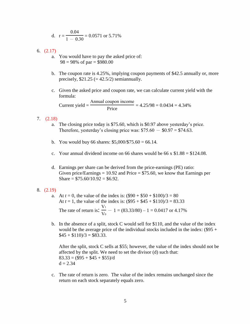
d. r =
- = 0.0571 or 5.71%
6. (2.17)
a. You would have to pay the asked price of:
98 = 98% of par = $980.00
b. The coupon rate is 4.25%, implying coupon payments of $42.5 annually or, more
precisely, $21.25 (= 42.5/2) semiannually.
c. Given the asked price and coupon rate, we can calculate current yield with the
formula:
Current yield = nnual coupon income
= 4.25/98 = 0.0434 = 4.34%
7. (2.18)
a. The closing price today is $75.60, which is $0.97 above yesterday’s price.
Therefore, yesterday’s closing price was: $ . - $0.97 = $74.63.
b. You would buy 66 shares: $5,000/$75.60 = 66.14.
c. Your annual dividend income on 66 shares would be 66 x $1.88 = $124.08.
d. Earnings per share can be derived from the price-earnings (PE) ratio:
Given price/Earnings = 10.92 and Price = $75.60, we know that Earnings per
Share = $75.60/10.92 = $6.92.
8. (2.19)
a. At t = 0, the value of the index is: ($90 + $50 + $100)/3 = 80
At t = 1, the value of the index is: ($95 + $45 + $110)/3 = 83.33
The rate of return is:
- 1 = (83.33/80) – 1 = 0.0417 or 4.17%
b. In the absence of a split, stock C would sell for $110, and the value of the index
would be the average price of the individual stocks included in the index: ($95 +
$45 + $110)/3 = $83.33.
After the split, stock C sells at $55; however, the value of the index should not be
affected by the split. We need to set the divisor (d) such that:
83.33 = ($95 + $45 + $55)/d
d = 2.34
c. The rate of return is zero. The value of the index remains unchanged since the
return on each stock separately equals zero.
6
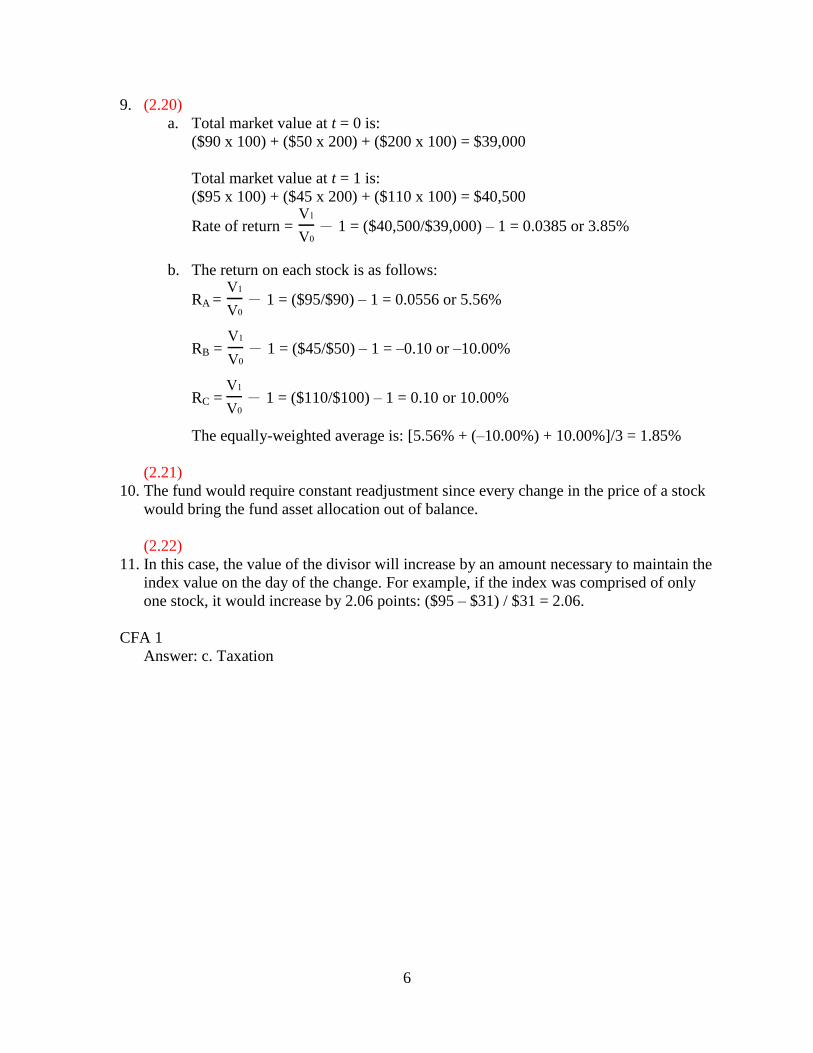
9. (2.20)
a. Total market value at t = 0 is:
($90 x 100) + ($50 x 200) + ($200 x 100) = $39,000
Total market value at t = 1 is:
($95 x 100) + ($45 x 200) + ($110 x 100) = $40,500
Rate of return =
- 1 = ($40,500/$39,000) – 1 = 0.0385 or 3.85%
b. The return on each stock is as follows:
RA =
- 1 = ($95/$90) – 1 = 0.0556 or 5.56%
RB =
- 1 = ($45/$50) – 1 = –0.10 or –10.00%
RC =
- 1 = ($110/$100) – 1 = 0.10 or 10.00%
The equally-weighted average is: [5.56% + (–10.00%) + 10.00%]/3 = 1.85%
(2.21)
10. The fund would require constant readjustment since every change in the price of a stock
would bring the fund asset allocation out of balance.
(2.22)
11. In this case, the value of the divisor will increase by an amount necessary to maintain the
index value on the day of the change. For example, if the index was comprised of only
one stock, it would increase by 2.06 points: ($95 – $31) / $31 = 2.06.
CFA 1
Answer: c. Taxation
7
Chapter 3
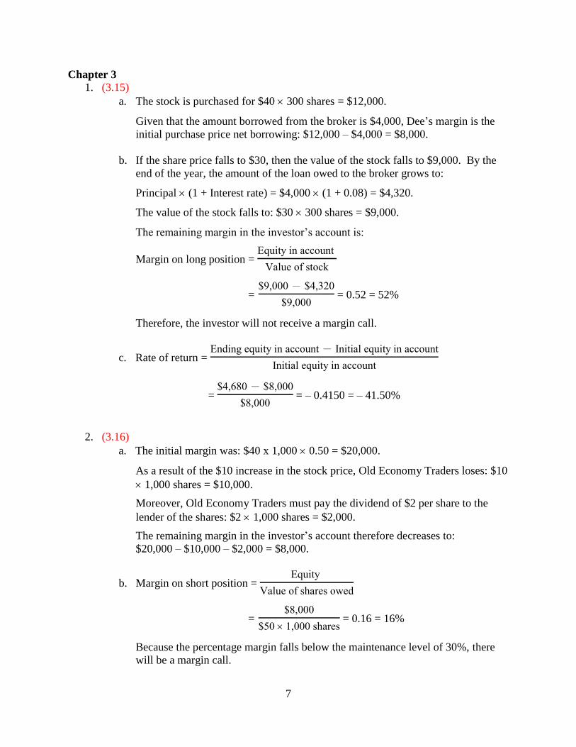
1. (3.15)
a. The stock is purchased for $40 300 shares = $12,000.
Given that the amount borrowed from the broker is $4,000, Dee’s margin is the
initial purchase price net borrowing: $12,000 – $4,000 = $8,000.
b. If the share price falls to $30, then the value of the stock falls to $9,000. By the
end of the year, the amount of the loan owed to the broker grows to:
Principal (1 + Interest rate) = $4,000 (1 + 0.08) = $4,320.
The value of the stock falls to: $30 300 shares = $9,000.
The remaining margin in the investor’s account is:
Margin on long position = quity in account
alue of stock
= $ , - $ ,
$ , = 0.52 = 52%
Therefore, the investor will not receive a margin call.
c. Rate of return = nding equity in account - nitial equity in account
nitial equity in account
= $ , - $ ,
$ , = – 0.4150 = – 41.50%
2. (3.16)
a. The initial margin was: $40 x 1,000 0.50 = $20,000.
As a result of the $10 increase in the stock price, Old Economy Traders loses: $10
1,000 shares = $10,000.
Moreover, Old Economy Traders must pay the dividend of $2 per share to the
lender of the shares: $2 1,000 shares = $2,000.
The remaining margin in the investor’s account therefore decreases to:
$20,000 – $10,000 – $2,000 = $8,000.
b. Margin on short position = quity
alue of shares owed
= $ ,
$ , shares = 0.16 = 16%
Because the percentage margin falls below the maintenance level of 30%, there
will be a margin call.
8
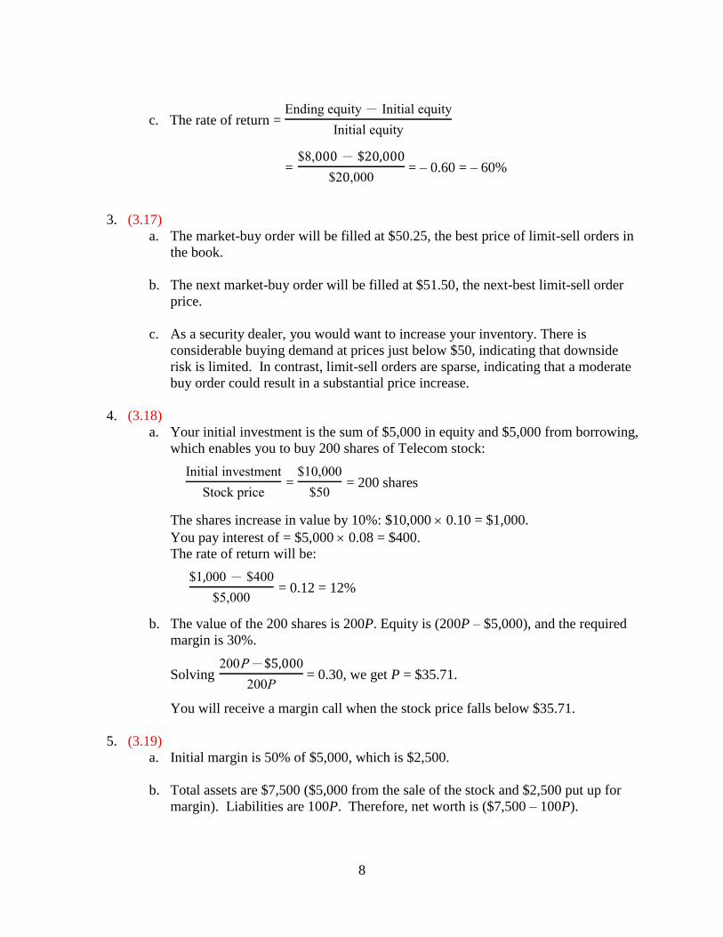
c. The rate of return = nding equity - nitial equity
nitial equity
= $ , -
$ , = – 0.60 = – 60%
3. (3.17)
a. The market-buy order will be filled at $50.25, the best price of limit-sell orders in
the book.
b. The next market-buy order will be filled at $51.50, the next-best limit-sell order
price.
c. As a security dealer, you would want to increase your inventory. There is
considerable buying demand at prices just below $50, indicating that downside
risk is limited. In contrast, limit-sell orders are sparse, indicating that a moderate
buy order could result in a substantial price increase.
4. (3.18)
a. Your initial investment is the sum of $5,000 in equity and $5,000 from borrowing,
which enables you to buy 200 shares of Telecom stock:
nitial investment
Stock price = $ ,
$ = 200 shares
The shares increase in value by 10%: $10,000 0.10 = $1,000.
You pay interest of = $5,000 0.08 = $400.
The rate of return will be:
$ - $
$ , = 0.12 = 12%
b. The value of the 200 shares is 200P. Equity is (200P – $5,000), and the required
margin is 30%.
Solving -
= 0.30, we get P = $35.71.
You will receive a margin call when the stock price falls below $35.71.
5. (3.19)
a. Initial margin is 50% of $5,000, which is $2,500.
b. Total assets are $7,500 ($5,000 from the sale of the stock and $2,500 put up for
margin). Liabilities are 100P. Therefore, net worth is ($7,500 – 100P).
9
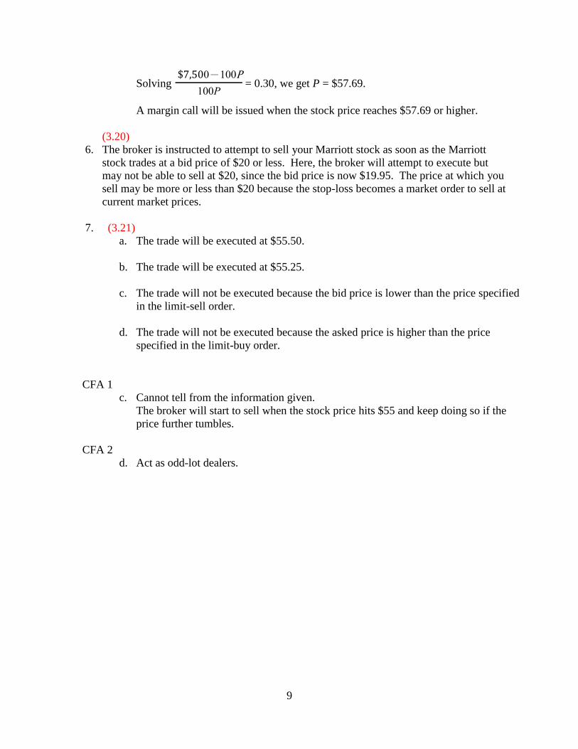
Solving -
= 0.30, we get P = $57.69.
A margin call will be issued when the stock price reaches $57.69 or higher.
(3.20)
6. The broker is instructed to attempt to sell your Marriott stock as soon as the Marriott
stock trades at a bid price of $20 or less. Here, the broker will attempt to execute but
may not be able to sell at $20, since the bid price is now $19.95. The price at which you
sell may be more or less than $20 because the stop-loss becomes a market order to sell at
current market prices.
7. (3.21)
a. The trade will be executed at $55.50.
b. The trade will be executed at $55.25.
c. The trade will not be executed because the bid price is lower than the price specified
in the limit-sell order.
d. The trade will not be executed because the asked price is higher than the price
specified in the limit-buy order.
CFA 1
c. Cannot tell from the information given.
The broker will start to sell when the stock price hits $55 and keep doing so if the
price further tumbles.
CFA 2
d. Act as odd-lot dealers.
10
Chapter 4
(4.11)
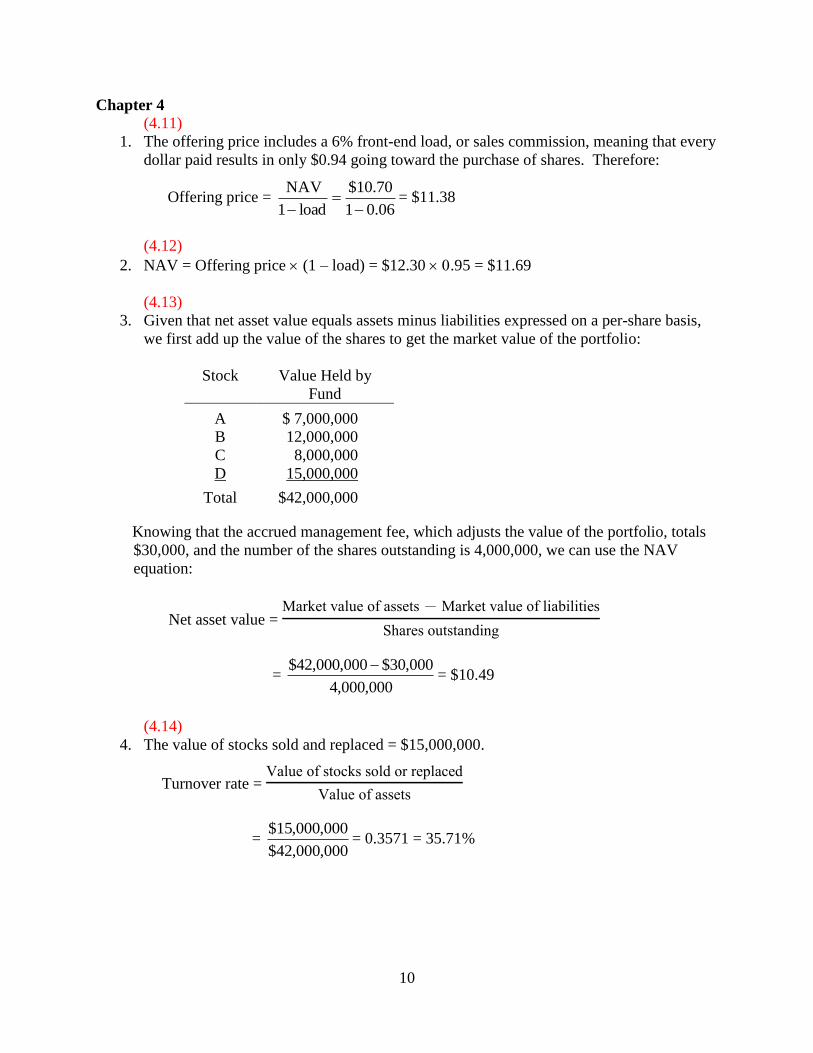
1. The offering price includes a 6% front-end load, or sales commission, meaning that every
dollar paid results in only $0.94 going toward the purchase of shares. Therefore:
Offering price = 06.01
70.10$
load1
NAV
= $11.38
(4.12)
2. NAV = Offering price (1 – load) = $12.30 .95 = $11.69
(4.13)
3. Given that net asset value equals assets minus liabilities expressed on a per-share basis,
we first add up the value of the shares to get the market value of the portfolio:
Stock Value Held by
Fund
A $ 7,000,000
B 12,000,000
C 8,000,000
D 15,000,000
Total $42,000,000
Knowing that the accrued management fee, which adjusts the value of the portfolio, totals
$30,000, and the number of the shares outstanding is 4,000,000, we can use the NAV
equation:
Net asset value = Market value of assets - Market value of liabilities
Shares outstanding
= 000,000,4
000,30$000,000,42$ = $10.49
(4.14)
4. The value of stocks sold and replaced = $15,000,000.
Turnover rate = alue of stocks sold or replaced
alue of assets
= 000,000,42$
000,000,15$= 0.3571 = 35.71%
11
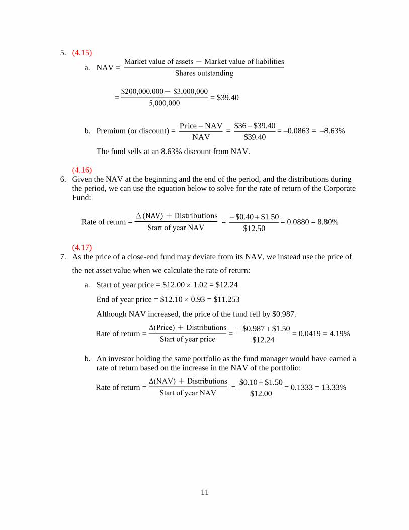
5. (4.15)
a. NAV = Market value of assets - Market value of liabilities
Shares outstanding
= $ , , - $ , ,
, , = $39.40
b. Premium (or discount) = NAV
NAVicePr =
40.39$
40.39$36$ = –0.0863 = –8.63%
The fund sells at an 8.63% discount from NAV.
(4.16)
6. Given the NAV at the beginning and the end of the period, and the distributions during
the period, we can use the equation below to solve for the rate of return of the Corporate
Fund:
Rate of return = s
Start of year =
50.12$
50.1$40.0$ = 0.0880 = 8.80%
(4.17)
7. As the price of a close-end fund may deviate from its NAV, we instead use the price of
the net asset value when we calculate the rate of return:
a. Start of year price = $12.00 1.02 = $12.24
End of year price = $12.10 0.93 = $11.253
Although NAV increased, the price of the fund fell by $0.987.
Rate of return = rice istributions
Start of year price =
24.12$
50.1$987.0$ = 0.0419 = 4.19%
b. An investor holding the same portfolio as the fund manager would have earned a
rate of return based on the increase in the NAV of the portfolio:
Rate of return = istributions
Start of year =
00.12$
50.1$10.0$ = 0.1333 = 13.33%
12
(4.18)
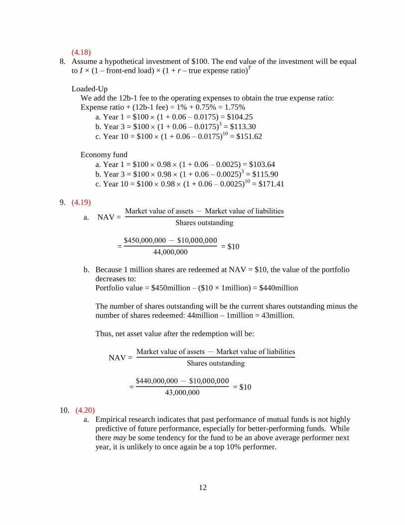
8. Assume a hypothetical investment of $100. The end value of the investment will be equal
to I × (1 – front-end load) × (1 + r – true expense ratio)T
Loaded-Up
We add the 12b-1 fee to the operating expenses to obtain the true expense ratio:
Expense ratio + (12b-1 fee) = 1% + 0.75% = 1.75%
a. Year 1 = $100 (1 + 0.06 – 0.0175) = $104.25
b. Year 3 = $100 (1 + 0.06 – 0.0175)3 = $113.30
c. Year 10 = $100 (1 + 0.06 – 0.0175)10
= $151.62
Economy fund
a. Year 1 = $100 0.98 (1 + 0.06 – 0.0025) = $103.64
b. Year 3 = $100 0.98 (1 + 0.06 – 0.0025)3 = $115.90
c. Year 10 = $100 0.98 (1 + 0.06 – 0.0025)10
= $171.41
9. (4.19)
a. NAV = Market value of assets - Market value of liabilities
Shares outstanding
= $ , , - $
, , = $10
b. Because 1 million shares are redeemed at NAV = $10, the value of the portfolio
decreases to:
Portfolio value = $450million – ($10 × 1million) = $440million
The number of shares outstanding will be the current shares outstanding minus the
number of shares redeemed: 44million – 1million = 43million.
Thus, net asset value after the redemption will be:
NAV = Market value of assets - Market value of liabilities
Shares outstanding
= $ , , - $
, , = $10
10. (4.20)
a. Empirical research indicates that past performance of mutual funds is not highly
predictive of future performance, especially for better-performing funds. While
there may be some tendency for the fund to be an above average performer next
year, it is unlikely to once again be a top 10% performer.

13
b. On the other hand, the evidence is more suggestive of a tendency for poor
performance to persist. This tendency is probably related to fund costs and
turnover rates. Thus if the fund is among the poorest performers, investors would
be concerned that the poor performance will persist.
(4.21)
11. Start of year NAV = Market value of assets - Market value of liabilities
Shares outstanding
= $ , ,
, , = $20
End of year NAV is based on the 8% price gain, less the 1% 12b-1 fee:
End of year NAV = $20 1.08 (1 – 0.01) = $21.384
Given the dividends per share is $0.20, we can calculate the rate of return using the
following equation:
Rate of return = istributions
Start of year
=
20$
20.0$20$384.21$ = 0.0792 = 7.92%
(4.22)
12. The excess of purchases over sales must be due to new inflows into the fund. Therefore,
$400 million of stock previously held by the fund was replaced by new holdings. So
turnover is:
Turnover rate = alue of stocks sold or replaced
alue of assets
= $ , ,
$ , , , = 0.1818 = 18.18%
(4.23)
13. Fees paid to investment managers were: 0.7% × $2.2 billion = $15.4 million.
Since the total expense ratio was 1.1% and the management fee was 0.7%, we conclude
that 0.4% must be for other expenses. Therefore, other administrative expenses were:
0.004 × $2.2 billion = $8.8 million.
14
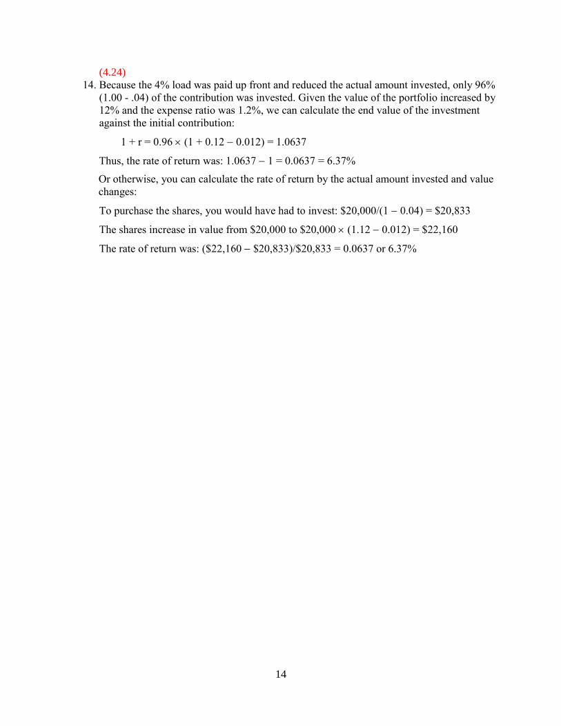
(4.24)
14. Because the 4% load was paid up front and reduced the actual amount invested, only 96%
(1.00 - .04) of the contribution was invested. Given the value of the portfolio increased by
12% and the expense ratio was 1.2%, we can calculate the end value of the investment
against the initial contribution:
1 + r = 0.96 (1 + 0.12 0.012) = 1.0637
Thus, the rate of return was: 1.0637 1 = 0.0637 = 6.37%
Or otherwise, you can calculate the rate of return by the actual amount invested and value
changes:
To purchase the shares, you would have had to invest: $20,000/(1 0.04) = $20,833
The shares increase in value from $20,000 to $20,000 (1.12 0.012) = $22,160
The rate of return was: ($22,160 $20,833)/$20,833 = 0.0637 or 6.37%

15
Chapter 5
(5.5)
1. Using Equation 5.6, we can calculate the mean of the HPR as:
E(r) = ∑ p s r s
= (0.3 0.44) + (0.4 0.14) + [0.3 (–0.16)] = 0.14 or
14%
Using Equation 5.7, we can calculate the variance as:
Var(r) = 2 = ∑ p s r s
– E(r)]
2
= [0.3 (0.44 – 0.14)2] + [0.4 (0.14 – 0.14)
2] + [0.3 (–0.16 – 0.14)
2]
= 0.054
Taking the square root of the variance, we get SD(r) = = √ ar r = √ . = 0.2324 or
23.24%
(5.6)
2. We use the below equation to calculate the holding period return of each scenario:
HPR = nding rice eginning rice ash ividend
ginning rice
a. The holding period returns for the three scenarios are:
Boom: (50 – 40 + 2)/40 = 0.30 = 30%
Normal: (43 – 40 + 1)/40 = 0.10 = 10%
Recession: (34 – 40 + 0.50)/40 = –0.1375 = –13.75%
E(HPR) = ∑ p s r s
= [(1/3) 0.30] + [(1/3) 0.10] + [(1/3) (–0.1375)]
= 0.0875 or 8.75%
Var(HPR) = ∑ p s r s
– E(r)]
2
= [(1/3) (0.30 – 0.0875)2] + [(1/3) (0.10 – 0.0875)2]
+ [(1/3) (–0.1375 – 0.0875)2]
= 0.031979
SD(r) = = √ ar r = 79.319 = 0.1788 or 17.88%
b. E(r) = (0.5 8.75%) + (0.5 4%) = 6.375%
= 0.5 17.88% = 8.94%

16
3. (5.7)
a. Time-weighted average returns are based on year-by-year rates of return.
Year Return = [(Capital gains + Dividend)/Price]
2010-2011 (110 – 100 + 4)/100 = 0.14 or 14.00%
2011-2012 (90 – 110 + 4)/110 = –0.1455 or –14.55%
2012-2013 (95 – 90 + 4)/90 = 0.10 or 10.00%
Arithmetic mean: [0.14 + (–0.1455) + 0.10]/3 = 0.0315 or 3.15%
Geometric mean: √ –
– 1
= 0.0233 or 2.33%
b.
Date
1/1/2010 1/1/2011 1/1/2012 1/1/2013
Net Cash Flow –300 –208 110 396
Time Net Cash flow Explanation
0 –300 Purchase of three shares at $100 per share
1 –208 Purchase of two shares at $110,
plus dividend income on three shares held
2 110 Dividends on five shares,
plus sale of one share at $90
3 396 Dividends on four shares,
plus sale of four shares at $95 per share
The dollar-weighted return is the internal rate of return that sets the sum of the
present value of each net cash flow to zero:
0 = –$300 + +
+
$
Dollar-weighted return = Internal rate of return = –0.1661%
4. (5.8)
a. Given that A = 4 and the projected standard deviation of the market return = 20%,
we can use the below equation to solve for the expected market risk premium:
A = 4 = verage rM rf
Sample M =
verage rM rf
E(rM) – rf = AM2 = 4 (0.20) = 0.16 or 16%
b. Solve E(rM) – rf = 0.09 = AM2 = A (0.20) , we can get
A = 0.09/0.04 = 2.25
17
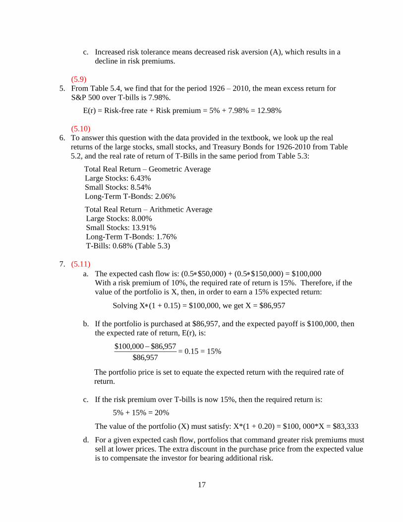
c. Increased risk tolerance means decreased risk aversion (A), which results in a
decline in risk premiums.
(5.9)
5. From Table 5.4, we find that for the period 1926 – 2010, the mean excess return for
S&P 500 over T-bills is 7.98%.
E(r) = Risk-free rate + Risk premium = 5% + 7.98% = 12.98%
(5.10)
6. To answer this question with the data provided in the textbook, we look up the real
returns of the large stocks, small stocks, and Treasury Bonds for 1926-2010 from Table
5.2, and the real rate of return of T-Bills in the same period from Table 5.3:
Total Real Return – Geometric Average
Large Stocks: 6.43%
Small Stocks: 8.54%
Long-Term T-Bonds: 2.06%
Total Real Return – Arithmetic Average
Large Stocks: 8.00%
Small Stocks: 13.91%
Long-Term T-Bonds: 1.76%
T-Bills: 0.68% (Table 5.3)
7. (5.11)
a. The expected cash flow is: (0.5$50,000) + (0.5$150,000) = $100,000
With a risk premium of 10%, the required rate of return is 15%. Therefore, if the
value of the portfolio is X, then, in order to earn a 15% expected return:
Solving X(1 + 0.15) = $100,000, we get X = $86,957
b. If the portfolio is purchased at $86,957, and the expected payoff is $100,000, then
the expected rate of return, E(r), is:
957,86$
957,86$000,100$ = 0.15 = 15%
The portfolio price is set to equate the expected return with the required rate of
return.
c. If the risk premium over T-bills is now 15%, then the required return is:
5% + 15% = 20%
The value of the portfolio (X) must satisfy: X*(1 + 0.20) = $100, 000*X = $83,333
d. For a given expected cash flow, portfolios that command greater risk premiums must
sell at lower prices. The extra discount in the purchase price from the expected value
is to compensate the investor for bearing additional risk.
18
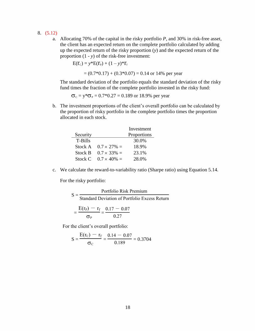
8. (5.12)
a. Allocating 70% of the capital in the risky portfolio P, and 30% in risk-free asset,
the client has an expected return on the complete portfolio calculated by adding
up the expected return of the risky proportion (y) and the expected return of the
proportion (1 - y) of the risk-free investment:
E(rC) = y*E(rP) + (1 – y)*rf
= (0.7*0.17) + (0.3*0.07) = 0.14 or 14% per year
The standard deviation of the portfolio equals the standard deviation of the risky
fund times the fraction of the complete portfolio invested in the risky fund:
C = y*P = 0.7*0.27 = 0.189 or 18.9% per year
b. The investment proportions of the client’s overall portfolio can be calculated by
the proportion of risky portfolio in the complete portfolio times the proportion
allocated in each stock.
Security
Investment
Proportions
T-Bills 30.0%
Stock A 0.7 27% = 18.9%
Stock B 0.7 33% = 23.1%
Stock C 0.7 40% = 28.0%
c. We calculate the reward-to-variability ratio (Sharpe ratio) using Equation 5.14.
For the risky portfolio:
S = ortfolio isk remium
Standard eviation of ortfolio xcess eturn
= r rf
=
For the client’s overall portfolio:
S = r rf
=
= 0.3704
19
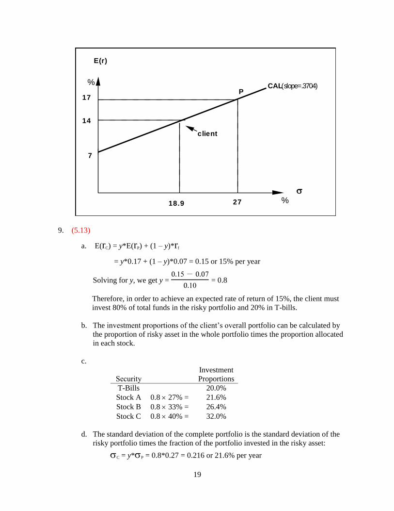
9. (5.13)
a. E(rC) = y*E(rP) + (1 – y)*rf
= y*0.17 + (1 – y)*0.07 = 0.15 or 15% per year
Solving for y, we get y =
= 0.8
Therefore, in order to achieve an expected rate of return of 15%, the client must
invest 80% of total funds in the risky portfolio and 20% in T-bills.
b. The investment proportions of the client’s overall portfolio can be calculated by
the proportion of risky asset in the whole portfolio times the proportion allocated
in each stock.
c.
Security
Investment
Proportions
T-Bills 20.0%
Stock A 0.8 27% = 21.6%
Stock B 0.8 33% = 26.4%
Stock C 0.8 40% = 32.0%
d. The standard deviation of the complete portfolio is the standard deviation of the
risky portfolio times the fraction of the portfolio invested in the risky asset:
C = y*P = 0.8*0.27 = 0.216 or 21.6% per year
E(r)
7
27
14
17P
CAL ( slope=.3704)%
% 18.9
client
20
10. (5.14)
a. Standard deviation of the complete portfolio= C = y*0.27
If the client wants the standard deviation to be equal or less than 20%, then:
y = (0.20/0.27) = 0.7407 = 74.07%
He should invest, at most, 74.07% in the risky fund.
b. E(rC) = rf + y*[E(rP) – rf] = 0.07 + 0.7407*0.10 = 0.1441 or 14.41%
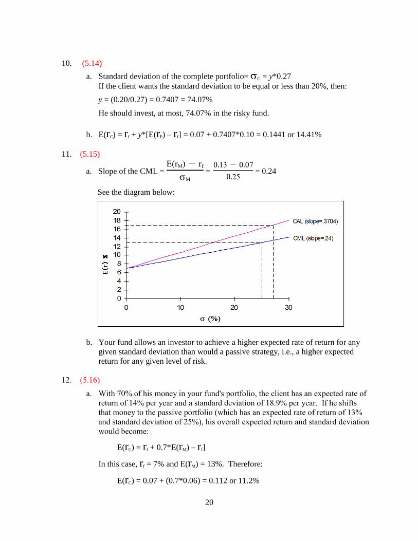
11. (5.15)
a. Slope of the CML = rM rf
M
=
= 0.24
See the diagram below:
b. Your fund allows an investor to achieve a higher expected rate of return for any
given standard deviation than would a passive strategy, i.e., a higher expected
return for any given level of risk.
12. (5.16)
a. With 70% of his money in your fund's portfolio, the client has an expected rate of
return of 14% per year and a standard deviation of 18.9% per year. If he shifts
that money to the passive portfolio (which has an expected rate of return of 13%
and standard deviation of 25%), his overall expected return and standard deviation
would become:
E(rC) = rf + 0.7*E(rM) – rf]
In this case, rf = 7% and E(rM) = 13%. Therefore:
E(rC) = 0.07 + (0.7*0.06) = 0.112 or 11.2%
21
The standard deviation of the complete portfolio using the passive portfolio would
be:
C = 0.7*M = 0.7*0.25 = 0.175 or 17.5%
Therefore, the shift entails a decline in the mean from 14% to 11.2% and a decline
in the standard deviation from 18.9% to 17.5%. Since both mean return and
standard deviation fall, it is not yet clear whether the move is beneficial. The
disadvantage of the shift is apparent from the fact that, if your client is willing to
accept an expected return on his total portfolio of 11.2%, he can achieve that return
with a lower standard deviation using your fund portfolio rather than the passive
portfolio. To achieve a target mean of 11.2%, we first write the mean of the
complete portfolio as a function of the proportions invested in your fund portfolio,
y:
E(rC) = 7% + y*(17% – 7%) = 7% + 10%*y
Because our target is E(rC) = 11.2%, the proportion that must be invested in your
fund is determined as follows:
11.2% = 7% + 10%*y, so y = .
= 0.42
The standard deviation of the portfolio would be:
C = y*27% = 0.42*27% = 11.34%
Thus, by using your portfolio, the same 11.2% expected rate of return can be
achieved with a standard deviation of only 11.34% as opposed to the standard
deviation of 17.5% using the passive portfolio.
b. The fee would reduce the reward-to-variability ratio, i.e., the slope of the CAL.
Clients will be indifferent between your fund and the passive portfolio if the slope
of the after-fee CAL and the CML are equal. Let f denote the fee:
Slope of CAL with fee =
=
Slope of CML (which requires no fee) =
= 0.24
Setting these slopes equal and solving for f:
= 0.24
10% – f = 27%*0.24 = 6.48%
f = 10%*6.48% = 3.52% per year

22
CFA 1
Answer: V(12/31/2011) = V(1/1/2005)*(1 + g)7 = $100,000*(1.05)
7 = $140,710.04
CFA 2
Answer: a. and b. are true. The standard deviation is non-negative.
CFA 3
nswer: c. etermines most of the portfolio’s return and volatility over time.
CFA 4
Answer: Investment 3.
For each portfolio: Utility = E(r) – (0.5 4 2)
Investment E(r) Utility
1 0.12 0.30 -0.0600
2 0.15 0.50 -0.3500
3 0.21 0.16 0.1588
4 0.24 0.21 0.1518
We choose the portfolio with the highest utility value.
CFA 5
Answer: Investment 4.
When an investor is risk neutral, A = 0 so that the portfolio with the highest utility is the
portfolio with the highest expected return.
CFA 6
nswer: b. nvestor’s aversion to risk.
23
Chapter 8
(8.11)
1. c. This is a predictable pattern of returns, which should not occur if the stock market is
weakly efficient.
(8.12)
2. c. This is a filter rule, a classic technical trading rule, which would appear to contradict the
weak form of the efficient market hypothesis.
(8.13)
3. c. The P/E ratio is public information so this observation would provide evidence against
the semi-strong form of the efficient market theory.
(8.14)
4. No, it is not more attractive as a possible purchase. Any value associated with dividend
predictability is already reflected in the stock price.
(8.15)
5. No, this is not a violation of the EMH. This empirical tendency does not provide investors
with a tool that will enable them to earn abnormal returns; in other words, it does not
suggest that investors are failing to use all available information. An investor could not
use this phenomenon to choose undervalued stocks today. The phenomenon instead
reflects the fact that dividends occur as a response to good performance. After the fact, the
stocks that happen to have performed the best will pay higher dividends, but this does not
imply that you can identify the best performers early enough to earn abnormal returns.
(8.16)
6. While positive beta stocks respond well to favorable new information about the
economy’s progress through the business cycle, the stock’s returns should be predictable
and should not show abnormal returns around already anticipated events. If a recovery, for
example, is already anticipated, the actual recovery is not news. The stock price should
already reflect the coming recovery. The level of the stock price will be unpredictable
only when responding to new information.
7. (8.17)
a. Consistent. Half of all managers should outperform the market based on pure
luck in any year.
b. Violation. This would be the basis for an "easy money" rule: Simply invest with
last year's best managers.
c. Consistent. Predictable volatility does not convey a means to earn abnormal
returns.
d. Violation. The abnormal performance ought to occur in January, when the
increased earnings are announced.
24
e. Violation. Reversals offer a means to earn easy money: Simply buy last week's
losers.
(8.18)
8. An anomaly is considered an EMH exception because there are historical data to
substantiate a claim that says anomalies have produced excess risk-adjusted abnormal
returns in the past. Several anomalies regarding fundamental analysis have been
uncovered. These include the P/E effect, the momentum effect, the small-firm-in-January
effect, the neglected- firm effect, post–earnings-announcement price drift, and the book-
to-market effect. Whether these anomalies represent market inefficiency or poorly
understood risk premiums is still a matter of debate. There are rational explanations for
each, but not everyone agrees on the explanation. One dominant explanation is that many
of these firms are also neglected firms, due to low trading volume, thus they are not part
of an efficient market or offer more risk as a result of their reduced liquidity.
CFA 1
Answer: b.
Public information constitutes semi-string efficiency, while the addition of private information
leads to strong form efficiency.
CFA 2
Answer: a.
The information should be absorbed instantly.
CFA 3
Answer: d.
All publically available information, including P/E ratio, should be absorbed in the price.
CFA 4
Answer: c.
Stocks producing abnormal excess returns will increase in price to eliminate the positive alpha.
CFA 5
Answer: c.
A random walk reflects no other information and is thus random.
CFA 6
Answer: d.
Unexpected results are by definition an anomaly.
25
Chapter 10
(10.12)
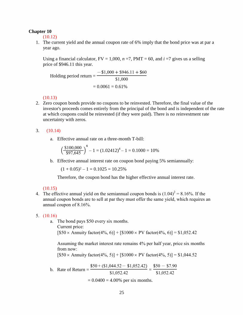
1. The current yield and the annual coupon rate of 6% imply that the bond price was at par a
year ago.
Using a financial calculator, FV = 1,000, n =7, PMT = 60, and i =7 gives us a selling
price of $946.11 this year.
Holding period return = - , $ .
$ ,
= 0.0061 = 0.61%
(10.13)
2. Zero coupon bonds provide no coupons to be reinvested. Therefore, the final value of the
investor's proceeds comes entirely from the principal of the bond and is independent of the rate
at which coupons could be reinvested (if they were paid). There is no reinvestment rate
uncertainty with zeros.
3. (10.14)
a. Effective annual rate on a three-month T-bill:
( $ , $ ,
)
– 1 = (1.02412)4 – 1 = 0.1000 = 10%
b. Effective annual interest rate on coupon bond paying 5% semiannually:
(1 + 0.05)2 – 1 = 0.1025 = 10.25%
Therefore, the coupon bond has the higher effective annual interest rate.
(10.15)
4. The effective annual yield on the semiannual coupon bonds is (1.04)2 = 8.16%. If the
annual coupon bonds are to sell at par they must offer the same yield, which requires an
annual coupon of 8.16%.
5. (10.16)
a. The bond pays $50 every six months.
Current price:
[$50 Annuity factor(4%, 6)] + [$1000 PV factor(4%, 6)] = $1,052.42
Assuming the market interest rate remains 4% per half year, price six months
from now:
[$50 Annuity factor(4%, 5)] + [$1000 PV factor(4%, 5)] = $1,044.52
b. Rate of Return = $ , . - , .
$ , . =
- $ .
$ , .
= 0.0400 = 4.00% per six months.

26
6. (10.17)
a. Use the following inputs: n = 40, FV = 1,000, PV = –950, PMT = 40. We will
find that the yield to maturity on a semi-annual basis is 4.26%. This implies a
bond equivalent yield to maturity of: 4.26% 2 = 8.52%
Effective annual yield to maturity = (1.0426)2 – 1 = 0.0870 = 8.70%
b. Since the bond is selling at par, the yield to maturity on a semi-annual basis is
the same as the semi-annual coupon, 4%. The bond equivalent yield to maturity
is 8%.
Effective annual yield to maturity = (1.04)2 – 1 = 0.0816 = 8.16%
c. Keeping other inputs unchanged but setting PV = –1,050, we find a bond
equivalent yield to maturity of 7.52%, or 3.76% on a semi-annual basis.
Effective annual yield to maturity = (1.0376)2 – 1 = 0.0766 = 7.66%
CFA 1
Answer:
a. (3) The yield on the callable bond must compensate the investor for the risk of
call.
Choice (1) is wrong because, although the owner of a callable bond receives
principal plus a premium in the event of a call, the interest rate at which he can
subsequently reinvest will be low. The low interest rate that makes it profitable
for the issuer to call the bond makes it a bad deal for the bond’s holder.
Choice (2) is wrong because a bond is more apt to be called when interest rates
are low. There will be an interest saving for the issuer only if rates are low.
b. (3)
c. (2)
d. (3)
CFA 2
Answer:
a. The maturity of each bond is 10 years, and we assume that coupons are paid
semiannually. Since both bonds are selling at par value, the current yield to maturity
for each bond is equal to its coupon rate.
If the yield declines by 1% to 5% (2.5% semiannual yield), the Sentinal bond will
increase in value to 107.79 [n=20; i = 2.5; FV = 100; PMT = 3].
The price of the Colina bond will increase, but only to the call price of 102. The
present value of scheduled payments is greater than 102, but the call price puts a
ceiling on the actual bond price.

27
b. If rates are expected to fall, the Sentinal bond is more attractive: Since it is not
subject to being called, its potential capital gains are higher. If rates are expected to
rise, Colina is a better investment. Its higher coupon (which presumably is
compensation to investors for the call feature of the bond) will provide a higher rate
of return than that of the Sentinal bond.
c. n increase in the volatility of rates increases the value of the firm’s option to call back the Colina bond. If rates go down, the firm can call the bond, which puts a cap
on possible capital gains. So, higher volatility makes the option to call back the
bond more valuable to the issuer. This makes the Colina bond less attractive to the
investor.
CFA 3
Answer
Market conversion value = Value if converted into stock
= 20.83 $28 = $583.24
Conversion premium = Bond value – Market conversion value
= $775 – $583.24 = $191.76
CFA 4
Answer:
a. The call provision requires the firm to offer a higher coupon (or higher promised
yield to maturity) on the bond in order to compensate the investor for the firm's
option to call back the bond at a specified call price if interest rates fall
sufficiently. Investors are willing to grant this valuable option to the issuer, but
only for a price that reflects the possibility that the bond will be called. That price
is the higher promised yield at which they are willing to buy the bond.
b. The call option reduces the expected life of the bond. If interest rates fall
substantially so that the likelihood of a call increases, investors will treat the bond
as if it will "mature" and be paid off at the call date, not at the stated maturity
date. On the other hand if rates rise, the bond must be paid off at the maturity
date, not later. This asymmetry means that the expected life of the bond will be
less than the stated maturity.
c. The advantage of a callable bond is the higher coupon (and higher promised yield
to maturity) when the bond is issued. If the bond is never called, then an investor
will earn a higher realized compound yield on a callable bond issued at par than
on a non-callable bond issued at par on the same date. The disadvantage of the
callable bond is the risk of call. If rates fall and the bond is called, then the
investor receives the call price and will have to reinvest the proceeds at interest
rates that are lower than the yield to maturity at which the bond was originally
issued. In this event, the firm's savings in interest payments are the investor's loss.
28
CFA 5
Answer:
a.
(1) Current yield = Coupon/Price = $70/$960 = 0.0729 = 7.29%
(2) YTM = 3.993% semiannually or 7.986% annual bond equivalent yield
[n = 10; PV = –960; FV = 1000; PMT = 35]
Then compute the interest rate.
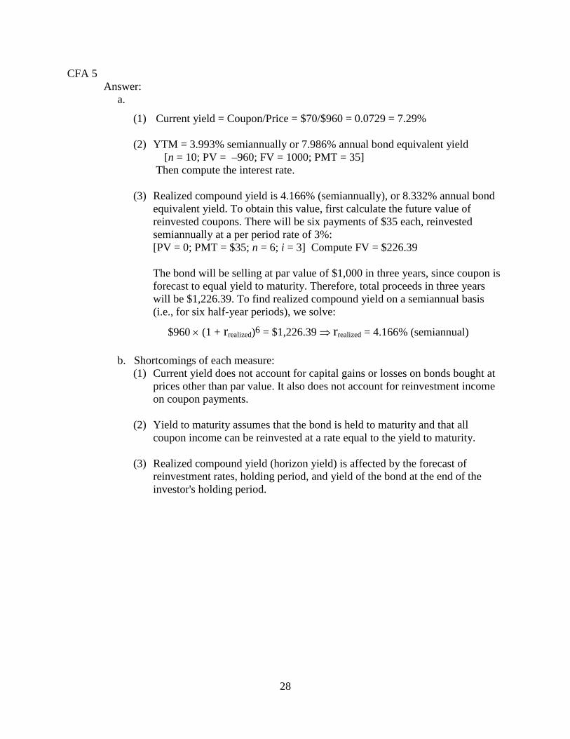
(3) Realized compound yield is 4.166% (semiannually), or 8.332% annual bond
equivalent yield. To obtain this value, first calculate the future value of
reinvested coupons. There will be six payments of $35 each, reinvested
semiannually at a per period rate of 3%:
[PV = 0; PMT = $35; n = 6; i = 3] Compute FV = $226.39
The bond will be selling at par value of $1,000 in three years, since coupon is
forecast to equal yield to maturity. Therefore, total proceeds in three years
will be $1,226.39. To find realized compound yield on a semiannual basis
(i.e., for six half-year periods), we solve:
$960 (1 + rrealized)6 = $1,226.39 rrealized = 4.166% (semiannual)
b. Shortcomings of each measure:
(1) Current yield does not account for capital gains or losses on bonds bought at
prices other than par value. It also does not account for reinvestment income
on coupon payments.
(2) Yield to maturity assumes that the bond is held to maturity and that all
coupon income can be reinvested at a rate equal to the yield to maturity.
(3) Realized compound yield (horizon yield) is affected by the forecast of
reinvestment rates, holding period, and yield of the bond at the end of the
investor's holding period.
29
Chapter 11
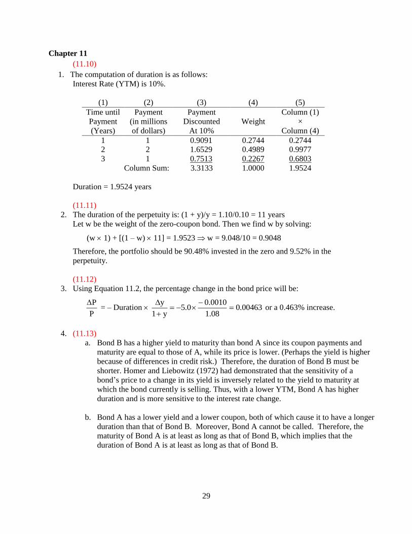
(11.10)
1. The computation of duration is as follows:
Interest Rate (YTM) is 10%.
(1) (2) (3) (4) (5)
Time until
Payment
(Years)
Payment
(in millions
of dollars)
Payment
Discounted
At 10%
Weight
Column (1)
×
Column (4)
1 1 0.9091 0.2744 0.2744 2 2 1.6529 0.4989 0.9977
3 1 0.7513 0.2267 0.6803
Column Sum: 3.3133 1.0000 1.9524
Duration = 1.9524 years
(11.11)
2. The duration of the perpetuity is: (1 + y)/y = 1.10/0.10 = 11 years
Let w be the weight of the zero-coupon bond. Then we find w by solving:
(w 1) + [(1 – w) 11] = 1.9523 w = 9.048/10 = 0.9048
Therefore, the portfolio should be 90.48% invested in the zero and 9.52% in the
perpetuity.
(11.12)
3. Using Equation 11.2, the percentage change in the bond price will be:
P
P = – Duration 00463.0
08.1
0010.00.5
y1
y
or a 0.463% increase.
4. (11.13)
a. Bond B has a higher yield to maturity than bond A since its coupon payments and
maturity are equal to those of A, while its price is lower. (Perhaps the yield is higher
because of differences in credit risk.) Therefore, the duration of Bond B must be
shorter. Homer and Liebowitz (1972) had demonstrated that the sensitivity of a
bond’s price to a change in its yield is inversely related to the yield to maturity at
which the bond currently is selling. Thus, with a lower YTM, Bond A has higher
duration and is more sensitive to the interest rate change.
b. Bond A has a lower yield and a lower coupon, both of which cause it to have a longer
duration than that of Bond B. Moreover, Bond A cannot be called. Therefore, the
maturity of Bond A is at least as long as that of Bond B, which implies that the
duration of Bond A is at least as long as that of Bond B.

30
CFA 1
Answer:
C: Highest maturity, zero coupon
D: Highest maturity, next-lowest coupon
A: Highest maturity, same coupon as remaining bonds (Bond B and E)
B: Lower yield to maturity than bond E
E: Highest coupon, shortest maturity, highest yield of all bonds
CFA 2
Answer:
a. Modified duration = YTM1
durationMacaulay
If the Macaulay duration is 10 years and the yield to maturity is 8%, then the
modified duration is: 10/1.08 = 9.26 years
b. For option-free coupon bonds, modified duration is better than maturity as a
measure of the bond’s sensitivity to changes in interest rates. Maturity considers
only the final cash flow, while modified duration includes other factors such as the
size and timing of coupon payments and the level of interest rates (yield to
maturity). Modified duration, unlike maturity, tells us the approximate proportional
change in the bond price for a given change in yield to maturity.
c. i. Modified duration increases as the coupon decreases.
ii. Modified duration decreases as maturity decreases.
CFA 10
Answer:
a. (4) A low coupon and a long maturity
b. (4) Zero, long
c. (4) All the above
d. (2) Great price volatility
31
Chapter 12
(12.13)
1. This exercise is left to the student.
(12.14)
2. Expansionary (i.e., looser) monetary policy to lower interest rates would help to stimulate
investment and expenditures on consumer durables. Expansionary fiscal policy (i.e.,
lower taxes, higher government spending, increased welfare transfers) would directly
stimulate aggregate demand.
(12.15)
3. A depreciating dollar makes imported cars more expensive and American cars cheaper to
foreign consumers. This should benefit the U.S. auto industry.
CFA 2
Answer:
a. The concept of an industrial life cycle refers to the tendency of most industries to
go through various stages of growth. The rate of growth, the competitive
environment, profit margins and pricing strategies tend to shift as an industry
moves from one stage to the next, although it is difficult to pinpoint exactly when
one stage has ended and the next begun.
The start-up stage is characterized by perceptions of a large potential market and
by high optimism for potential profits. In this stage, however, there is usually a
high failure rate. In the second stage, often called rapid growth or consolidation,
growth is high and accelerating, markets broaden, unit costs decline, and quality
improves. In this stage, industry leaders begin to emerge. The third stage, usually
called the maturity stage, is characterized by decelerating growth caused by such
things as maturing markets and/or competitive inroads by other products. Finally,
an industry reaches a stage of relative decline, in which sales slow or even
decline.
Product pricing, profitability, and industry competitive structure often vary by
phase. Thus, for example, the first phase usually encompasses high product
prices, high costs (R&D, marketing, etc.) and a (temporary) monopolistic industry
structure. In phase two (consolidation stage), new entrants begin to appear and
costs fall rapidly due to the learning curve. Prices generally do not fall as rapidly,
however, allowing profit margins to increase. In phase three (maturity stage),
growth begins to slow as the product or service begins to saturate the market, and
margins are eroded by significant price reductions. In the final stage, cumulative
industry production is so high that production costs have stopped declining, profit
margins are thin (assuming competition exists), and the fate of the industry
depends on the extent of replacement demand and the existence of substitute
products/services.
32
b. The passenger car business in the United States has probably entered the final
stage in the industrial life cycle because normalized growth is quite low. The
information processing business, on the other hand, is undoubtedly earlier in the
cycle. Depending on whether or not growth is still accelerating, it is either in the
second or third stage.
c. Cars: In the final phases of the life cycle, demand tends to be price sensitive.
Thus, Universal can not raise prices without losing volume. Moreover, given the
industry’s maturity, cost structures are likely to be similar for all competitors, and
any price cuts can be matched immediately. Thus, Universal’s car business is
boxed in: Product pricing is determined by the market, and the company is a
“price-taker.”
Idata: Idata should have much more pricing flexibility given that it is in an earlier
phase of the industrial life cycle. Demand is growing faster than supply, and,
depending on the presence and/or actions of an industry leader, Idata may price
high in order to maximize current profits and generate cash for product
development, or price low in an effort to gain market share.
CFA 3
Answer:
a. A basic premise of the business cycle approach to investing is that stock prices
anticipate fluctuations in the business cycle. For example, there is evidence that
stock prices tend to move about six months ahead of the economy. In fact, stock
prices are a leading indicator for the economy.
Over the course of a business cycle, this approach to investing would work
roughly as follows. As the top of a business cycle is perceived to be approaching,
stocks purchased should not be vulnerable to a recession. When a downturn is
perceived to be at hand, stock holdings should be reduced, with proceeds invested
in fixed-income securities. Once the recession has matured to some extent, and
interest rates fall, bond prices will rise. As it is perceived that the recession is
about to end, profits should be taken in the bonds and proceeds reinvested in
stocks, particularly stocks with high beta that are in cyclical industries.
Abnormal returns will generally be earned only if these asset allocation switches
are timed better than those of other investors. Switches made after the turning
points may not lead to excess returns.
b. Based on the business cycle approach to investment timing, the ideal time to
invest in a cyclical stock like a passenger car company would be just before the
end of a recession. f the recovery is already underway, dams’s recommendation
would be too late. The equities market generally anticipates changes in the
economic cycle. Therefore, since the “recovery is underway,” the price of
Universal Auto should already reflect the anticipated improvements in the
economy.
33
Chapter 13
(13.13)
1. FCFE1 = FCFF – Interest expenses(1 – tc) + Increases in net debt
= $205 – $22 (1 – 0.35) + $3 = $193.70 (million)
Market value of equity = F F
k - g =
.
- = $2,152.22 (million)
(13.14)
2. Cost of equity = rf + E(Risk premium) = 7% + 4% = 11%
Because the dividends are expected to be constant every year, the price can be calculated
as the no-growth-value per share:
P0 =
ke = $ .
= $19.09
(13.15)
3. k = rf + β [E(rM) – rf ] = 0.05 + 1.5 (0.10 – 0.05) = 0.125 or 12.5%
Therefore:
P0 =
k - g =
$ .
- = $29.41
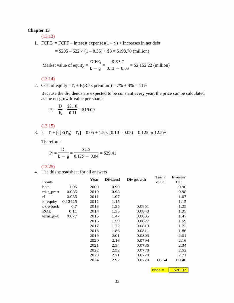
(13.25)
4. Use this spreadsheet for all answers
Inputs Year Dividend Div growth
Term
value
Investor
CF
beta 1.05 2009 0.90 0.90
mkt_prem 0.085 2010 0.98 0.98
rf 0.035 2011 1.07 1.07
k_equity 0.12425 2012 1.15 1.15
plowback 0.7 2013 1.25 0.0851 1.25
ROE 0.11 2014 1.35 0.0843 1.35
term_gwth 0.077 2015 1.47 0.0835 1.47
2016 1.59 0.0827 1.59
2017 1.72 0.0819 1.72
2018 1.86 0.0811 1.86
2019 2.01 0.0803 2.01
2020 2.16 0.0794 2.16
2021 2.34 0.0786 2.34
2022 2.52 0.0778 2.52
2023 2.71 0.0770 2.71
2024 2.92 0.0770 66.54 69.46
Price = $20.07
34
a. Price = $20.62
b. Price = $18.95
c. Price = $20.07
CFA 1
Answer:
a. This director is confused. In the context of the constant growth model, it is true that
price is higher when dividends are higher holding everything else (including
dividend growth) constant. But everything else will not be constant. If the firm
raises the dividend payout rate, then the growth rate (g) will fall, and stock price
will not necessarily rise. In fact, if ROE > k, price will fall.
b. i. An increase in dividend payout reduces the sustainable growth rate as fewer
funds are reinvested in the firm.
ii. The sustainable growth rate is (ROE plowback), which falls as the plowback
ratio falls. The increased dividend payout rate reduces the growth rate of book
value for the same reason—fewer funds are reinvested in the firm.
CFA 2
Answer:
a. It is true that NewSoft sells at higher multiples of earnings and book value than
Capital. But this difference may be justified by NewSoft's higher expected growth
rate of earnings and dividends. NewSoft is in a growing market with abundant
profit and growth opportunities. Capital is in a mature industry with fewer growth
prospects. Both the price-earnings and price-book ratios reflect the prospect of
growth opportunities, indicating that the ratios for these firms do not necessarily
imply mispricing.
b. The most important weakness of the constant-growth dividend discount model in
this application is that it assumes a perpetual constant growth rate of dividends.
While dividends may be on a steady growth path for Capital, which is a more mature
firm, that is far less likely to be a realistic assumption for NewSoft.
c. NewSoft should be valued using a multi-stage DDM, which allows for rapid growth
in the early years, but also recognizes that growth must ultimately slow to a more
sustainable rate.
CFA 3
Answer:
a. The industry’s estimated / can be computed using the following model:
P0/E1 = payout ratio/(r g)
However, since r and g are not explicitly given, they must be computed using the
following formulas:
35
gind = ROE retention rate = 0.25 0.40 = 0.10
rind = government bond yield + ( industry beta equity risk premium)
= 0.06 + (1.2 0.05) = 0.12
Therefore:
P0/E1 = 0.60/(0.12 0.10) = 30.0
b.
i. Forecast growth in real GDP would cause P/E ratios to be generally higher for
Country A. Higher expected growth in GDP implies higher earnings growth
and a higher P/E.
ii. Government bond yield would cause P/E ratios to be generally higher for
Country B. A lower government bond yield implies a lower risk-free rate and
therefore a higher P/E.
iii. Equity risk premium would cause P/E ratios to be generally higher for
Country B. A lower equity risk premium implies a lower required return and
a higher P/E.
CFA 4
Answer:
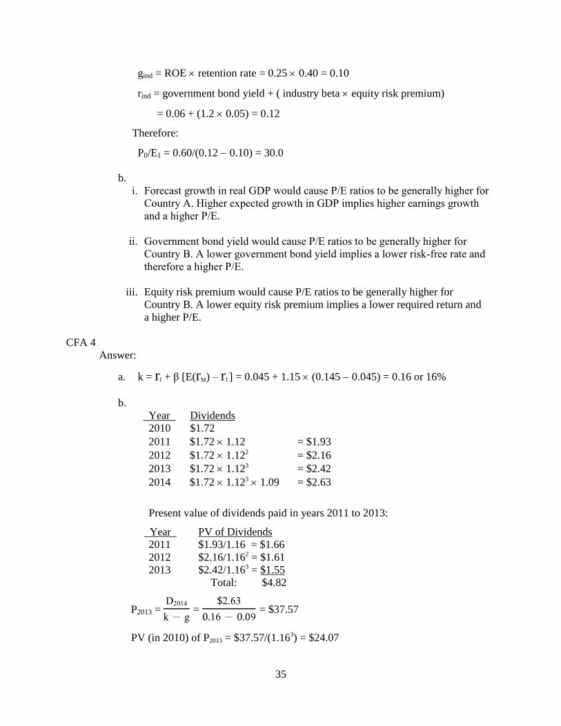
a. k = rf + β [E(rM) – rf ] = 0.045 + 1.15 (0.145 0.045) = 0.16 or 16%
b.
Year Dividends
2010 $1.72
2011 $1.72 1.12 = $1.93
2012 $1.72 1.122 = $2.16
2013 $1.72 1.123 = $2.42
2014 $1.72 1.123 1.09 = $2.63
Present value of dividends paid in years 2011 to 2013:
Year PV of Dividends
2011 $1.93/1.16 = $1.66
2012 $2.16/1.162 = $1.61
2013 $2.42/1.163 = $1.55
Total: $4.82
P2013 =
k - g =
.
- = $37.57
PV (in 2010) of P2013 = $37.57/(1.163) = $24.07

36
Intrinsic value of stock = $4.82 + $24.07 = $28.89
c. The table presented in the problem indicates that QuickBrush is selling below
intrinsic value, while we have just shown that SmileWhite is selling somewhat
above the estimated intrinsic value. Based on this analysis, QuickBrush offers
the potential for considerable abnormal returns, while SmileWhite offers slightly
below-market risk-adjusted returns.
d. Strengths of two-stage DDM compared to constant growth DDM:
The two-stage model allows for separate valuation of two distinct periods in a
company’s future. This approach can accommodate life cycle effects. It also
can avoid the difficulties posed when the initial growth rate is higher than the
discount rate.
The two-stage model allows for an initial period of above-sustainable growth.
It allows the analyst to make use of her expectations as to when growth may
shift to a more sustainable level.
A weakness of all DDMs is that they are all very sensitive to input values.
Small changes in k or g can imply large changes in estimated intrinsic value.
These inputs are difficult to measure.
37
Chapter 15
1. (15.4)
Cost Payoff Profit
Call option, X = 160 15.00 5.00 -10.00
Put option, X = 160 9.40 0.00 -9.40
Call option, X = 165 11.70 0.00 -11.70
Put option, X = 165 10.85 0.00 -10.85
Call option, X = 170 8.93 0.00 -8.93
Put option, X = 170 13.00 5.00 -8.00
(15.5)
2. If the stock price drops to zero, you will make $160 – $2.62 per stock, or $157.38. Given
100 units per contract, the total potential profit is $15,738.
3. (15.9)
a. i. A long straddle produces gains if prices move up or down and limited losses if
prices do not move. A short straddle produces significant losses if prices move
significantly up or down. A bullish spread produces limited gains if prices move
up.
b. i. Long put positions gain when stock prices fall and produce very limited losses
if prices instead rise. Short calls also gain when stock prices fall but create losses
if prices instead rise. The other two positions will not protect the portfolio should
prices fall.
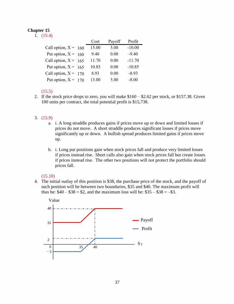
(15.10)
4. The initial outlay of this position is $38, the purchase price of the stock, and the payoff of
such position will be between two boundaries, $35 and $40. The maximum profit will
thus be: $40 – $38 = $2, and the maximum loss will be: $35 – $38 = –$3.
S T
35
40
Payoff
Profit
3
2
Value
0 40 35
38
(15.11)
5. The collar involves purchasing a put for $3 and selling a call for $2. The initial outlay is
$1.
a. ST = $30
Value at expiration = Value of call + Value of put + Value of stock
= $0 + ($35 – $30) + $30 = $35
Given 5,000 shares, the total net proceeds will be:
(Final Value – Original Investment) # of shares
= ($35 – $1) 5,000 = $170,000
Net proceeds without using collar = ST # of shares
= $30 5,000 = $150,000
b. ST = $40
Value at expiration = Value of call + Value of put + Value of stock
= 0 + 0 + $40 = $40
Given 5,000 shares, the total net proceeds will be:
(Final value – Original investment) # of shares
= ($40 – $1) 5,000 = $195,000
Net proceeds without using collar = ST # of shares
= $40 5,000 = $200,000
c. ST = $50
Value at expiration = Value of call + Value of put + Value of stock
= ($45 – $50) + 0 + $50 =$45
Given 5,000 shares, the total net proceeds will be:
(Final value – Original investment) # of shares
= ($45 – $1) 5,000 = $220,000
Net proceeds without using collar = ST # of shares
= $50 5,000 = $250,000
With the initial outlay of $1, the collar locks the net proceeds per share in between the
lower bound of $34 and the upper bound of $44. Given 5,000 shares, the total net
proceeds will be between $170,000 and $220,000 when the position is closed. If we
simply continued to hold the shares without using the collar, the upside potential is not
limited but the downside is not protected.
39
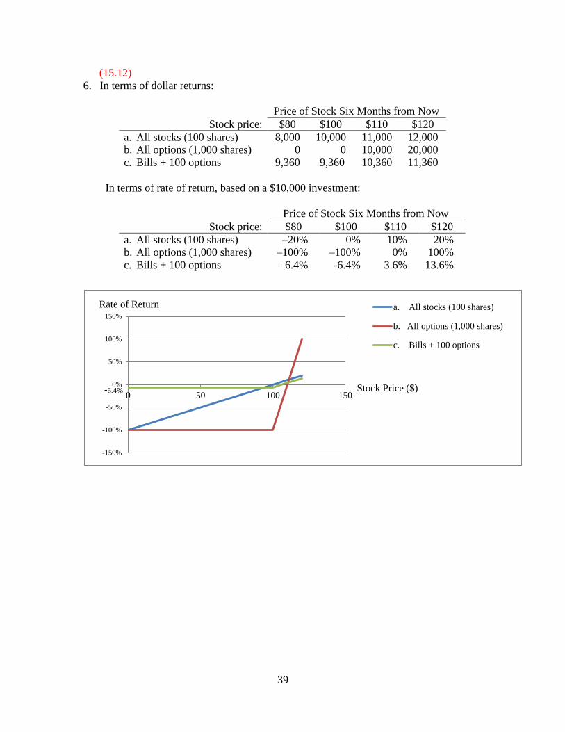
(15.12)
6. In terms of dollar returns:
Price of Stock Six Months from Now
Stock price: $80 $100 $110 $120
a. All stocks (100 shares) 8,000 10,000 11,000 12,000 b. All options (1,000 shares) 0 0 10,000 20,000
c. Bills + 100 options 9,360 9,360 10,360 11,360
In terms of rate of return, based on a $10,000 investment:
Price of Stock Six Months from Now
Stock price: $80 $100 $110 $120
a. All stocks (100 shares) –20% 0% 10% 20% b. All options (1,000 shares) –100% –100% 0% 100%
c. Bills + 100 options –6.4% -6.4% 3.6% 13.6%
-150%
-100%
-50%
0%
50%
100%
150%
0 50 100 150
a. All stocks (100 shares)
b. All options (1,000 shares)
c. Bills + 100 options
Rate of Return
Stock Price ($) -6.4%
40
Chapter 17
(17.2)
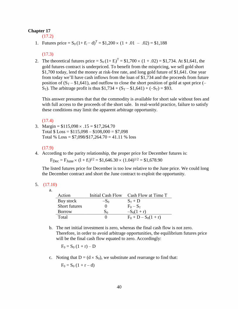
1. Futures price = S0 (1+ rf − d)T = $1,200 (1 + .01 – .02) = $1,188
(17.3)
2. The theoretical futures price = S0 (1+ rf)T = $1,700 (1 + .02) = $1,734. At $1,641, the
gold futures contract is underpriced. To benefit from the mispricing, we sell gold short
$1,700 today, lend the money at risk-free rate, and long gold future of $1,641. One year
from today we’ll have cash inflows from the loan of $1,734 and the proceeds from future
position of (ST – $1,641), and outflow to close the short position of gold at spot price (–
ST). The arbitrage profit is thus $1,734 + (ST – $1,641) + (–ST) = $93.
This answer presumes that that the commodity is available for short sale without fees and
with full access to the proceeds of the short sale. In real-world practice, failure to satisfy
these conditions may limit the apparent arbitrage opportunity.
(17.4)
3. Margin = $115,098 .15 = $17,264.70
Total $ Loss = $115,098 – $108,000 = $7,098
Total % Loss = $7,098/$17,264.70 = 41.11 % loss
(17.9)
4. According to the parity relationship, the proper price for December futures is:
FDec = FJune (l + rf)l/2 = $1,646.30 (1.04)1/2 = $1,678.90
The listed futures price for December is too low relative to the June price. We could long
the December contract and short the June contract to exploit the opportunity.
5. (17.10)
a.
Action Initial Cash Flow Cash Flow at Time T
Buy stock –S0 ST + D Short futures 0 F0 – ST
Borrow S0 –S0(1 + r)
Total 0 F0 + D – S0(1 + r)
b. The net initial investment is zero, whereas the final cash flow is not zero.
Therefore, in order to avoid arbitrage opportunities, the equilibrium futures price
will be the final cash flow equated to zero. Accordingly:
F0 = S0 (1 + r) – D
c. Noting that D = (d S0), we substitute and rearrange to find that:
F0 = S0 (1 + r – d)

41
6. (17.11)
a. F0 = S0 (1 + rf)T = $150 1.03 = $154.50
b. F0 = S0 (1 + rf)T = $150 (1.03)
3 = $163.91
c. F0 = S0 (1 + rf)T = $150 (1.05)
3 = $173.64
CFA 1
Answer:
a. Contrasts
CFA 2
Answer:
d. Maintenance margin
CFA 3
Answer:
Total losses may amount to $3,500 before a margin call is received. Each contract calls
for delivery of 5,000 ounces. Before a margin call is received, the price per ounce can
increase by: $3,500/5,000 = $ .70
The futures price at this point would be: $28 + $ .70 = $28.70

42
Chapter 18
7. (18.5)
a.
E(r)
Portfolio A 11% 10% .8 Portfolio B 14% 31% 1.5
Market index 12% 20% 1.0
Risk-free asset 6% 0% 0.0
The alphas for the two portfolios are:
αA = E(rA) – required return predicted by CAPM
= .11 – [.06 + .8 (.12 – .06)] = 0.2%
αB = E(rB) – required return predicted by CAPM
= .14 – [.06 + 1.5 (.12 – .06)] = –1.0%
Ideally, you would want to take a long position in Portfolio A and a short position
in Portfolio B.
b. If you hold only one of the two portfolios, then the Sharpe measure is the
appropriate criterion:
SA = r - rf
= . - .
. = .5
SB = r - rf
= . - .
. = .26
Therefore, using the Sharpe criterion, Portfolio A is preferred.
(18.6)
8. We first distinguish between timing ability and selection ability. The intercept of the
scatter diagram is a measure of stock selection ability. If the manager tends to have a
positive excess return even when the market’s performance is merely “neutral” i.e., the
market has zero excess return) then we conclude that the manager has, on average, made
good stock picks. In other words, stock selection must be the source of the positive
excess returns.
Timing ability is indicated by the curvature of the plotted line. Lines which become
steeper as you move to the right of the graph show good timing ability. The steeper slope
shows that the manager maintained higher portfolio sensitivity to market swings (i.e., a
higher beta) in periods when the market performed well. This ability to choose more
market-sensitive securities in anticipation of market upturns is the essence of good
timing. In contrast, a declining slope as you move to the right indicates that the portfolio
was more sensitive to the market when the market performed poorly and less sensitive to
the market when the market performed well. This indicates poor timing.

43
We can therefore classify performance ability for the four managers as follows:
Selection Ability Timing Ability
A Bad Good
B Good Good
C Good Bad
D Bad Bad
9. (18.7)
a. Actual: (.70 .02) + (.20 .01) + (.10 .005) = .0165 = 1.65%
Bogey: (.60 .025) + (.30 .012) + (.10 .005) = .0191 = 1.91%
Underperformance = .0191 – .0165 = .0026 = .26%
b. Security Selection:
(1) (2) (3) (4) (5) = (3) (4)
Market Portfolio
Performance
Index
Performance
Excess
Performance
Manager’s
Portfolio
Weight
Contribution
Equity 2.0% 2.5% – .5% .70 – .35%
Bonds 1.0% 1.2% – .2% .20 – .04%
Cash .5% .5% 0% .10 .00%
Contribution of Security Selection: – .39%
c. Asset Allocation:
(1) (2) (3) (4) (5) = (3) (4)
Market Actual
Weight
Benchmark
Weight
Excess
Weight Index Return Contribution
Equity .70 .60 .10 2.5% .25% Bonds .20 .30 – .10 1.2% – .12%
Cash .10 .10 0 .5% 0%
Contribution of Asset Allocation: .13%
Summary
Security selection – .39%
Asset allocation .13%
Excess performance – .26%
CFA 1
Answer:
d. Russell 2000 Index
44
CFA 2
Answer:
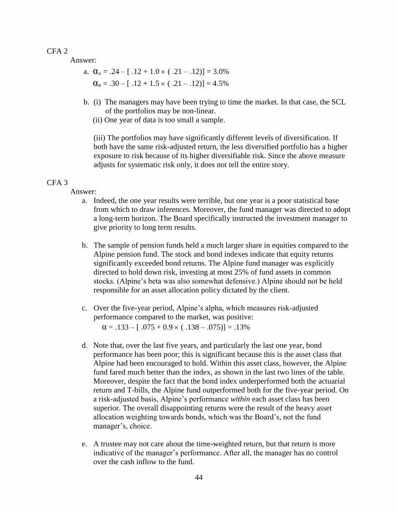
a. αA = .24 – [ .12 + 1.0 ( .21 – .12)] = 3.0%
αB = .30 – [ .12 + 1.5 ( .21 – .12)] = 4.5%
b. (i) The managers may have been trying to time the market. In that case, the SCL
of the portfolios may be non-linear.
(ii) One year of data is too small a sample.
(iii) The portfolios may have significantly different levels of diversification. If
both have the same risk-adjusted return, the less diversified portfolio has a higher
exposure to risk because of its higher diversifiable risk. Since the above measure
adjusts for systematic risk only, it does not tell the entire story.
CFA 3
Answer:
a. Indeed, the one year results were terrible, but one year is a poor statistical base
from which to draw inferences. Moreover, the fund manager was directed to adopt
a long-term horizon. The Board specifically instructed the investment manager to
give priority to long term results.
b. The sample of pension funds held a much larger share in equities compared to the
Alpine pension fund. The stock and bond indexes indicate that equity returns
significantly exceeded bond returns. The Alpine fund manager was explicitly
directed to hold down risk, investing at most 25% of fund assets in common
stocks. lpine’s beta was also somewhat defensive. lpine should not be held
responsible for an asset allocation policy dictated by the client.
c. Over the five-year period, lpine’s alpha, which measures risk-adjusted
performance compared to the market, was positive:
α = .133 – [ .075 + 0.9 ( .138 – .075)] = .13%
d. Note that, over the last five years, and particularly the last one year, bond
performance has been poor; this is significant because this is the asset class that
Alpine had been encouraged to hold. Within this asset class, however, the Alpine
fund fared much better than the index, as shown in the last two lines of the table.
Moreover, despite the fact that the bond index underperformed both the actuarial
return and T-bills, the Alpine fund outperformed both for the five-year period. On
a risk-adjusted basis, lpine’s performance within each asset class has been
superior. The overall disappointing returns were the result of the heavy asset
allocation weighting towards bonds, which was the oard’s, not the fund
manager’s, choice.
e. A trustee may not care about the time-weighted return, but that return is more
indicative of the manager’s performance. fter all, the manager has no control
over the cash inflow to the fund.
45
CFA 4
Answer:
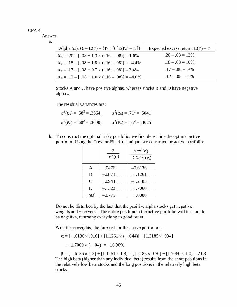
a.
Alpha (): αi = E(ri) – {rf + βi [E(rM) – rf ]} Expected excess return: E(ri) – rf
αA = .20 – [ .08 + 1.3 ( .16 – .08)] = 1.6% .20 – .08 = 12%
αB = .18 – [ .08 + 1.8 ( .16 – .08)] = –4.4% .18 – .08 = 10%
αC = .17 – [ .08 + 0.7 ( .16 – .08)] = 3.4% .17 – .08 = 9%
αD = .12 – [ .08 + 1.0 ( .16 – .08)] = –4.0% .12 – .08 = 4%
Stocks A and C have positive alphas, whereas stocks B and D have negative
alphas.
The residual variances are:
2(eA) = .58
2 = .3364;
2(eB) = .71
2 = .5041
2(eC) = .60
2 = .3600;
2(eD) = .55
2 = .3025
b. To construct the optimal risky portfolio, we first determine the optimal active
portfolio. Using the Treynor-Black technique, we construct the active portfolio:
αi i
A .0476 –0.6136
B –.0873 1.1261
C .0944 –1.2185
D –.1322 1.7060
Total –.0775 1.0000
Do not be disturbed by the fact that the positive alpha stocks get negative
weights and vice versa. The entire position in the active portfolio will turn out to
be negative, returning everything to good order.
With these weights, the forecast for the active portfolio is:
α = [– .6136 .016] + [1.1261 (– .044)] – [1.2185 .034]
+ [1.7060 (– .04)] = –16.90%
= [– .6136 1.3] + [1.1261 1.8] – [1.2185 0.70] + [1.7060 1.0] = 2.08
The high beta (higher than any individual beta) results from the short positions in
the relatively low beta stocks and the long positions in the relatively high beta
stocks.
46
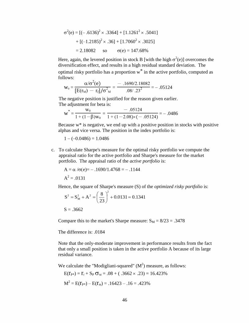
2(e) = [(– .6136)
2 .3364] + [1.1261
2 .5041]
+ [(–1.2185)2 .36] + [1.7060
2 .3025]
= 2.18082 so e = 147.68%
Here, again, the levered position in stock B [with the high 2(e)] overcomes the
diversification effect, and results in a high residual standard deviation. The
optimal risky portfolio has a proportion w* in the active portfolio, computed as
follows:
w0 =
rM - rf M
= - . / .
. / . = – .05124
The negative position is justified for the reason given earlier.
The adjustment for beta is:
w* =
w
- w
= - .
- . - = – .0486
Because w* is negative, we end up with a positive position in stocks with positive
alphas and vice versa. The position in the index portfolio is:
1 – (–0.0486) = 1.0486
c. To calculate Sharpe's measure for the optimal risky portfolio we compute the
appraisal ratio for the active portfolio and Sharpe's measure for the market
portfolio. The appraisal ratio of the active portfolio is:
A = /e)= – .1690/1.4768 = – .1144
A2 = .0131
Hence, the square of Sharpe's measure (S) of the optimized risky portfolio is:
1341.00131.023
8ASS
2
22
M
2
S = .3662
Compare this to the market's Sharpe measure: SM = 8/23 = .3478
The difference is: .0184
Note that the only-moderate improvement in performance results from the fact
that only a small position is taken in the active portfolio A because of its large
residual variance.
We calculate the "Modigliani-squared" (M2) measure, as follows:
E(rP*) = rf + SP M = .08 + ( .3662 .23) = 16.423%
M2 = E(rP*) – E(rM) = .16423 – .16 = .423%
47
Chapter 19
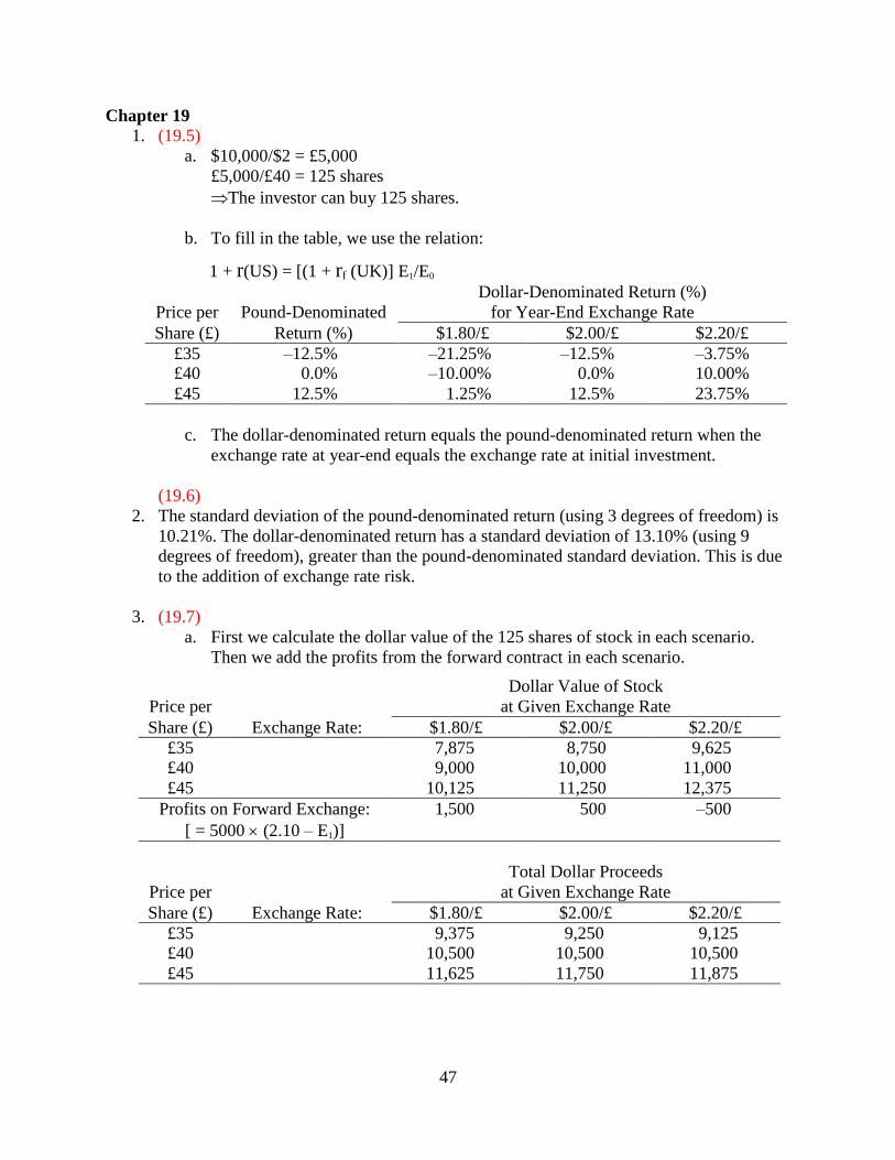
1. (19.5)
a. $10,000/$2 = £5,000
£5,000/£40 = 125 shares
The investor can buy 125 shares.
b. To fill in the table, we use the relation:
1 + r(US) = [(1 + rf (UK)] E1/E0
Price per
Pound-Denominated
Dollar-Denominated Return (%)
for Year-End Exchange Rate
Share (£) Return (%) $1.80/£ $2.00/£ $2.20/£
£35 –12.5% –21.25% –12.5% –3.75% £40 0.0% –10.00% 0.0% 10.00%
£45 12.5% 1.25% 12.5% 23.75%
c. The dollar-denominated return equals the pound-denominated return when the
exchange rate at year-end equals the exchange rate at initial investment.
(19.6)
2. The standard deviation of the pound-denominated return (using 3 degrees of freedom) is
10.21%. The dollar-denominated return has a standard deviation of 13.10% (using 9
degrees of freedom), greater than the pound-denominated standard deviation. This is due
to the addition of exchange rate risk.
3. (19.7)
a. First we calculate the dollar value of the 125 shares of stock in each scenario.
Then we add the profits from the forward contract in each scenario.
Price per
Dollar Value of Stock
at Given Exchange Rate
Share (£) Exchange Rate: $1.80/£ $2.00/£ $2.20/£
£35 7,875 8,750 9,625 £40 9,000 10,000 11,000
£45 10,125 11,250 12,375
Profits on Forward Exchange:
[ = 5000 (2.10 – E1)]
1,500 500 –500
Price per
Total Dollar Proceeds
at Given Exchange Rate
Share (£) Exchange Rate: $1.80/£ $2.00/£ $2.20/£
£35 9,375 9,250 9,125 £40 10,500 10,500 10,500
£45 11,625 11,750 11,875
48
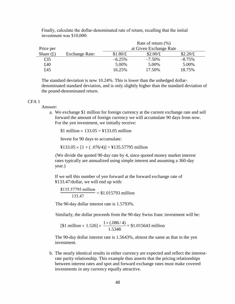
Finally, calculate the dollar-denominated rate of return, recalling that the initial
investment was $10,000:
Price per
Rate of return (%)
at Given Exchange Rate
Share (£) Exchange Rate: $1.80/£ $2.00/£ $2.20/£
£35 –6.25% –7.50% –8.75% £40 5.00% 5.00% 5.00%
£45 16.25% 17.50% 18.75%
The standard deviation is now 10.24%. This is lower than the unhedged dollar-
denominated standard deviation, and is only slightly higher than the standard deviation of
the pound-denominated return.
CFA 1
Answer:
a. We exchange $1 million for foreign currency at the current exchange rate and sell
forward the amount of foreign currency we will accumulate 90 days from now.
For the yen investment, we initially receive:
$1 million 133.05 = ¥133.05 million
Invest for 90 days to accumulate:
¥133.05 [1 + ( .076/4)] = ¥135.57795 million
(We divide the quoted 90-day rate by 4, since quoted money market interest
rates typically are annualized using simple interest and assuming a 360-day
year.)
If we sell this number of yen forward at the forward exchange rate of
¥133.47/dollar, we will end up with:
. million
. = $1.015793 million
The 90-day dollar interest rate is 1.5793%.
Similarly, the dollar proceeds from the 90-day Swiss franc investment will be:
[$1 million 1.526] 5348.1
)4/086(.1= $1.015643 million
The 90-day dollar interest rate is 1.5643%, almost the same as that in the yen
investment.
b. The nearly identical results in either currency are expected and reflect the interest-
rate parity relationship. This example thus asserts that the pricing relationships
between interest rates and spot and forward exchange rates must make covered
investments in any currency equally attractive.
49
c. The dollar-hedged rate of return on default-free government securities in Japan is
1.5793% and in Switzerland is 1.5643%. Therefore, the 90-day interest rate
available on U.S. government securities must be between 1.5643% and 1.5793%.
This corresponds to an annual rate between 6.2572% and 6.3172%, which is less
than the APR in Japan or Switzerland. (For consistency with our earlier
calculations, we annualize the 90-day rate using the convention of the money
market, assuming a 360-day year and simple interest). The lower interest rate in
the U.S. makes sense, as the relationship between forward and spot exchange rates
indicates that the U.S. dollar is expected to appreciate against both the Japanese
yen and the Swiss franc.
CFA 2
a. The primary rationale is the opportunity for diversification. Factors that contribute
to low correlations of stock returns across national boundaries are:
i. imperfect correlation of business cycles
ii. imperfect correlation of interest rates
iii. imperfect correlation of inflation rates
iv. exchange rate volatility
b. Obstacles to international investing are:
i. Availability of information, including insufficient data on which to base
investment decisions. It is difficult to interpret and evaluate data that is
different in form and/or content than the routinely available and widely
understood U.S. data. Also, much foreign data is reported with a
considerable lag.
ii. Liquidity, in terms of the ability to buy or sell, in size and in a timely
manner, without affecting the market price. Most foreign exchanges offer
(relative to U.S. norms) limited trading, and experience greater price
volatility. Moreover, only a (relatively) small number of individual foreign
stocks enjoy liquidity comparable to that in the U.S., although this situation
is improving steadily.
iii. Transaction costs, particularly when viewed as a combination of
commission plus spread plus market impact costs, are well above U.S. levels
in most foreign markets. This, of course, adversely affects return
realization.
iv. Political risk.
v. Foreign currency risk, although to a great extent, this can be hedged.
c. The asset-class performance data for this particular period reveal that non-U.S. dollar
bonds provided a small incremental return advantage over U.S. dollar bonds, but at a
considerably higher level of risk. Each category of fixed income assets outperformed
the S&P 500 Index measure of U.S. equity results with regard to both risk and return,
which is certainly an unexpected outcome. Within the equity area, non-U.S. stocks,
represented by the EAFE Index, outperformed U.S. stocks by a considerable margin
with only slightly more risk. In contrast to U.S. equities, this asset category
50
performed as it should relative to fixed income assets, providing more return for the
higher risk involved.
Concerning the Account Performance Index, its position on the graph reveals an
aggregate outcome that is superior to the sum of its component parts. To some extent,
this is due to the beneficial effect on performance resulting from multi-market
diversification and the differential covariances involved. In this case, the portfolio
manager(s) (apparently) achieved an on-balance positive alpha, adding to total
portfolio return by their actions. The addition of international (i.e., non-U.S.)
securities to a portfolio that would otherwise have held only domestic (U.S.)
securities clearly worked to the advantage of this fund over this time period.