Naval Research Laboratory Washington, DC 20375-5320

NRL/MR/6110--99-8342

Software for Generating Synthetic Passive Fourier Transform Infrared Interferograms and Single-beam Spectra

RONALD E. SHAFFER

Chemical Dynamics and Diagnostics Branch Chemistry Division

ROGER J. COMBS

U.S. Army ERDEC Aberdeen Proving Ground, MD

CD CD

February 12, 1999

©

©

Approved for public release; distribution unlimited.

REPORT DOCUMENTATION PAGE Form Approved OMB No. 0704-0188

Public reporting burden for this collection of information is estimated to average 1 hour per response, including the time for reviewing instructions, searching existing data sources, gathering and maintaining the data needed, and completing and reviewing the collection of information. Send comments regarding this burden estimate or any other aspect of this collection of information, including suggestions for reducing this burden, to Washington Headquarters Services, Directorate for Information Operations^and Reports 1215 Jefferson Davis Highway Suite 1204 Arlington, VA 22202-4302, and to the Office of Management and Budget. Paperwork Reduction Project (0704-0188), Washington, DC 20503.

1. AGENCY USE ONLY (Leave Blank) 2. REPORT DATE

February 12, 1999

3. REPORT TYPE AND DATES COVERED

Final Report October 1997-September 1998

4. TITLE AND SUBTITLE

Software for Generating Synthetic Passive Fourier Transform Infrared Interferograms and Single-beam Spectra

5. FUNDING NUMBERS

6. AUTHOR(S)

Ronald E. Shaffer and Roger J. Combs

7. PERFORMING ORGANIZATION NAME(S) AND ADDRESS(ES)

Naval Research Laboratory Washington, DC 20375-5320

8. PERFORMING ORGANIZATION REPORT NUMBER

NRL/MR/6110-99-8342

9. SPONSORING/MONITORING AGENCY NAME(S) AND ADDRESS(ES)

U.S. Army ERDEC Aberdeen Proving Ground, MD 21010-5423 Arlington, VA 22242-5160

10. SPONSORING/MONITORING AGENCY REPORT NUMBER

11. SUPPLEMENTARY NOTES

*U.S. Army ERDEC, Aberdeen Proving Ground, MD 21010-5423

12a. DISTRIBUTION/AVAILABILITY STATEMENT

Approved for public release; distribution unlimited.

12b. DISTRIBUTION CODE

A

13. ABSTRACT (Maximum 200 words)

Software routines for generating synthetic Fourier transform infrared (FT-IR) spectra and interferograms are documented. Infrared radiative transfer models for passive FT-IR spectroscopy are furnished, providing a basis for simulating realistic spectral data. Laboratory passive FT-IR spectra and interferograms are shown to validate the software performance. Due to variability in reported absorption coefficients, it is found that simulated data are not a replacement for either laboratory or field quantitative measurements. However, the synthetic data capability provides a versatile resource for examining experimental results and a flexible tool for chemometric research into various signal processing strategies for passive FT-IR spectroscopy. The software routines in the "FTIRTooIbox" are written in MATLAB. Complete program source code listings are provided in

the appendix.

14. SUBJECT TERMS

FTIR MATLAB Infrared Radiative model Simulation

15. NUMBER OF PAGES

60

16. PRICE CODE

17. SECURITY CLASSIFICATION OF REPORT

UNCLASSIFIED

18. SECURITY CLASSIFICATION OF THIS PAGE

UNCLASSIFIED

19. SECURITY CLASSIFICATION OF ABSTRACT

UNCLASSIFIED

20. LIMITATION OF ABSTRACT

UL

NSN 7540-01-280-5500 Standard Form 298 (Rev. 2-89]

Prescribed by ANSI Std 239-18

298-102

CONTENTS

INTRODUCTION 1

EXPERIMENTAL 2

THEORY 3

RESULTS AND DISCUSSION 7

CONCLUSIONS 12

ACKNOWLEDGMENTS 13

REFERENCES 14

APPENDIX 27

in

Software for Generating Synthetic Passive Fourier Transform Infrared Interferograms and Single-beam Spectra

INTRODUCTION

The remote detection and identification of toxic vapors in the atmosphere provides significant information for assessing both the military and environmental impact of these materials. One powerful analytical tool for these remote sensing applications is passive Fourier transform infrared (FT-IR) spectroscopy [1-4]. Passive FT-IR remote sensing is widely documented for a variety of open-air monitoring scenarios [5-7]. Unlike the traditional bistatic and monostatic active FT-IR spectrometer configurations that each require an elevated temperature infrared (IR) source, the passive FT-IR sensor configuration relies solely on the ambient radiance difference between the target vapor and the background such as terrain, water, sky, or some combination. For atmospheric monitoring and other open-air applications, the passive configuration provides a distinct advantage in deployment over the traditional active configurations.

The traditional limitations to the passive measurement have been the lack of a stable infrared background and the occurrence of weak spectral signatures for the analytes of interest. Recently, workers have demonstrated great promise in overcoming these limitations through the application of advanced signal processing and pattern recognition algorithms to raw FT-IR interferograms [8-11]. While powerful, these methods require specific information about the analytes of interest and robust signal processing schemes since each interferogram point contain components of all spectral frequencies. Traditional data analysis methodology designed for spectral-domain processing of infrared absorbance spectra is well characterized and visually intuitive. However, the analysis of interferometric data is not as straightforward. The interferogram-based analysis scheme takes advantage of the fact that signals from wide spectral bands (i.e., the frequency-domain or spectral-domain) dampen faster in the interferogram (time-domain) than narrow spectral bands. By coupling a frequency selective time-domain digital filter with a judiciously selected interferogram segment, analyte specific detection and quantification is often performed, even for complex mixtures such as the analysis of blood glucose [12]. Since the concepts and terminology of this methodology are not as well-established, this approach requires greater experimentation than spectral-based methods for optimizing many of the signal processing and pattern recognition parameters. Time-domain interferogram processing (i.e., digital filtering and pattern recognition) relies more heavily on robust data sets that provide a global description of the experimental and instrumental conditions.

The need for statistically complete data sets for passive FT-IR remote sensing implies that extensive data collection efforts for feasibility studies are necessary. However, controlled releases of many toxic gases are heavily restricted. Controlled releases are necessary for verification and quantification (i.e., ground truth). These experiments typically consists of vapor releases with a portable emission stack [13]. In these experiments it is often difficult to know exact vapor plume concentrations and dimensions due to potential variations in meteorological conditions and limitations imposed by the FT-IR sensor field of view. To fully understand and model these controlled releases requires the ability to account for (1) incomplete filling of the FT-IR

Manuscript approved January 26, 1999.

spectrometer field of view, (2) heterogeneous plume composition/temperature profiles, and (3) various background scene radiances.

One approach to quantifying the importance of the variances in vapor plume generation is to model the effects using single-beam spectra and interferograms that have been generated synthetically [14]. Synthetic spectral generation provides a means of assessing a wide variety of experimental conditions and promises to allow determination of optimal experimental designs for performing controlled open-air releases. Recent papers in the literature have reported various methods for computing synthetic data using simple radiometric models for passive FT-IR remote sensing [14- 16]. These radiometric models have been widely reported in the literature and have served as the basis for signal processing schemes designed to overcome the severe background variation present in the passive infrared measurement [17,18]. This report focuses on these semi-empirical radiative models and document the MATLAB-based software necessary for synthetic single-beam spectra and interferogram generation from library reference absorbance spectra.

EXPERIMENTAL

The FT-IR data used in this report were collected on two Midac Outfielder FTIR emission spectrometers (units 145 and 175, Midac, Corp., Irvine, CA). This spectrometer design is upon a flex-pivot "porch swing" Michelson interferometer. The detector spectral response was restricted to the 8-12 ^m atmospheric window. All interferograms consisted of 1024 points sampled at every eighth zero-crossing of the reference He-Ne laser. The maximum observable frequency was 1974.75 cm"1 and the point spacing in the single-beam spectra was approximately 4 cm"1. For validation of radiometric models, interferograms were collected under laboratory conditions in the passive FT-IR configuration. In the laboratory setup, an external blackbody source was positioned to ensure that it filled the entire field of view of the FT-IR spectrometer. Changing the blackbody source temperature permitted simulation of background radiance levels. Groups of 50 consecutive interferograms were acquired and subsequently averaged for each specific blackbody radiance temperature. This or similar laboratory experimental configurations have been employed in several other studies [9,10,19,20].

Additional interferograms were obtained from unit 175 with an infrared gas cell located in the field of view of the spectrometer prior to the blackbody source. At each blackbody temperature setting, 50 interferograms were collected with a known concentration of 1, 1, 1, trichloroethane (TCA) in the cell, while another 50 were collected with the cell filled with clean air. TCA was introduced into the gas cell as a liquid through a stopcock with the use of a digital microsyringe. The TCA liquid quickly evaporated to fill the cell. The concentration was determined based on the amount of liquid introduced and the pressure, temperature, and volume of the cell. Using this method of sample introduction, it is possible that some of the vapor can escape the cell before the stopcock can be closed. However, this method is certainly sufficient for qualitative analysis. Comparison to library spectra is difficult due to the presence of potential concentration errors which are reflected as errors in absorbance values.

Library absorbance spectra were obtained from the AEDC/U.S. EPA data base [21]. The library spectra were reduced from -0.25 cm"1 point spacing to 2 cm"1 point spacing (4 cm"1 resolution) by convolving with an instrument line function using software

provided by AEDC/EPA. To ensure correct registration with the Midac collected single- beam spectra, the deresolution was followed by cubic spline interpolation.

All calculations were performed with routines written in the commercial software package MATLAB (Mathworks, Inc., Natick, MA, version 5.2) on a Dual-processor 200 MHz Pentium Pro computer (Micron Electronics, Inc., Nampa, ID) running Windows NT (Microsoft, Inc., Richland, WA, version 4.0). The interpolation and random number generator routines used in the programs are internal MATLAB functions. The remaining program functions were written by the one of the authors (RES).

THEORY

Passive Infrared Spectroscopy

The fundamental basis for passive infrared spectroscopy is the theory of radiative transfer (radiation theory). Radiative transfer models allow the calculation of the energy reaching an IR detector in terms of spectral radiance. Since the spectral units and terminology used by chemists and physicists often differ, where possible this report relies on the symbols, nomenclature, and units as outlined in the Infrared Handbook [22]. The radiative model that is developed in this report is independent of the infrared instrumentation type (dispersive or FT-IR) used. The infrared spectral units (radiation variables) are usually given in terms of wavelength (X) for a dispersive instrument and wavenumber (v) for an FT-IR. In this report, we will use X for the general case and v for non-dispersive cases specific to FT-IR spectrometry.

The primary principal governing radiative transfer is that the radiance (L) emitted by any surface is Planck's theoretical blackbody function L*(k,T) scaled by the emissivity e(X),

L(A) = e(X) x L*(A, T) (1)

where T is the temperature of the material. A blackbody is defined as a perfect radiator and is dependent solely upon the temperature of the material (i.e., e = 1). Although no material found in nature is a perfect blackbody, they are a central component to passive infrared radiometric modeling. Emissivity is an intrinsic property of the material and is defined as the ratio of the radiance of a given body to that of a perfect blackbody. A material that has an emissivity which is independent of X is often called a gray body, while those with an emissivity that varies with X are termed spectral bodies. When radiance is incident upon a material, some of it is transmitted, some absorbed or emitted, and some is reflected. The total power law states that the sum of the transraittance (x), reflectance (p), and emittance is equal to unity. Since gases are usually nonreflective in the infrared, e(X) can be rewritten in terms of transmittance for purposes of passive IR model development (i.e., e(X) = 1 - x (X)).

The radiation incident on a passive IR sensor is the sum of the individual radiances from (1) the background, (2) the target gas cloud, and (3) the intervening atmospheric gases. Figure 1 depicts two potential measurement scenarios. One configuration is an FT-IR spectrometer mounted on an aircraft measuring a vapor plume contrasted against a background. Another scenario features a ground-based FT-IR

spectrometer observing a gas emanating from a hot smoke stack against a cold sky background.

Flanigan visualized the radiative transfer problem as a set of parallel layers orthogonal to the line of sight of the sensor [2,15,16]. Using Fig. 1 as an example, the first layer is the background to vapor plume (far field); the second layer consists of the vapor plume (consisting of the target analyte); and the final layer is the intervening atmosphere between the plume and the sensor (near field). Each layer attenuates the radiation passed to it from the previous layer. Flanigan expressed this relationship simply as

P = [TtxaLbg + (1-x,xa)LJxB, (2)

where P is power of the light incident on the sensor, xt is the target cloud transmittance, xa is the transmittance of the atmosphere, Ug is the radiance of the background, Lt is the radiance of the target cloud, and B is a parameter related to the optical collection efficiency of the passive sensor (i.e., the product of the collector area and solid acceptance angle). The target cloud transmittance is xt = exp(-<xc/) where a is the absorptivity (m2/mg) of the target gas and c is the concentration of the gas (mg/m3), and / is the optical pathlength (m) of the cloud. The target cloud absorbance is A = -log(tt) = 0.434(ac/). These equations assume that the target vapor fills the spectrometer field of view and negligible radiance losses occur due to scattering. If the collection efficiency of the sensor is ignored, eq. (2) can be rewritten in terms of the spectral radiance coming from the scene (Lx),

Lx = [Xt Xa Lbg + (1 - x, Ta) LJ. (3)

For simplicity, it is assumed that Ug and l_t are perfect blackbodies that are represented by Planck's function (L*). These radiances depend solely on temperatures of the background (Tbg) and the analyte plume (Tt) respectively.

One practical implication of the passive IR model is that the temperature difference between the target cloud (Tt) and the background (Tbg) must be significant for the infrared chemical signature of the analytes in the gas cloud to reach the sensor. If Tt

= Tug then eq. (3) reduces to Lx= Lbg. Thus, a challenging detection problem occurs when (1) the concentration or pathlength of the target gas is small (i.e., minimal xt) or (2) the temperature difference between the background and the cloud is small (i.e., L, - Lbg is minimal). The radiance model also explains why emission infrared features are found when the analyte vapor plume temperature is hotter than the background and absorbance features are seen when the background is hotter than the plume.

Generation of Synthetic FT-IR Spectra

The passive IR model given in eq. (3) can be used to generate synthetic single- beam FT-IR spectra and interferograms as follows:

1'. Equation (1) can be used to estimate the spectral radiance from the gas cloud and the background (Ug and Lt). Since the emittance is assumed to be equal to unity, Ug and Lt are easily computed at each wavenumber from Planck's blackbody equation

* C,xv3

L(v,T) = - exp(-^-—)-l

where Ci and C2 are the first and second radiation constants computed as

d = 2hc2 = 1.191 x 10"12 W/cm2 sr (cm"1)4 (5) and

C2=hc/k=1.439 Kern. (6)

Flanigan reported that MODTRAN can also be used for computing Ug [15]. The estimated radiance is based on the integration of Tbg across the MODTRAN path using the U.S. standard atmosphere model.

2. The target cloud transmittance (xt) can be obtained from one of many different sources such as laboratory collections, commercially available spectral libraries, or theoretical approaches [23]. Regardless of where the absorption coefficients (a) are obtained, for studying various passive FT-IR remote sensing scenarios, a must be scaled at each v to produce the desired cl. According the Hanst spectral library manual, dividing a library spectrum by its listed cl product will provide a good approximation to the absorption coefficients of the gas [24]. The library spectrum is essentially a one-point calibration model. If multiple gases are present in the cloud, their absorptivities are additive (assumes that no chemical interactions took place, which may cause nonlinearities). Once the absorption spectrum is created with the desired gases at the proper cl, it is converted to a transmission spectrum (xt) for use in eq. (3).

3. The atmospheric transmittance (xa) term can be ignored in certain applications involving low-altitude airborne or ground-based measurements where the distance between the gas cloud and the sensor is small. In cases where this assumption is not warranted, atmospheric transmittance and radiance software such as LOWTRAN or MODTRAN can be used to estimate xa [15, 25, 26].

4. If necessary, interpolate the xt, xa, Ug, and L, spectra so that they fall on the same wavenumber axis (i.e., have identical point spacing). If the spectral resolution of the target application is much different than the resolution of the xa and xt spectra, then deresolution prior to interpolation is necessary.

5. Compute the apparent spectral radiance (Lx) using eq. (3) and the products from step 4.

6. For the synthetic spectra to have any realistic value, the spectra need to have some noise component. According to Flanigan, noise can be added to the synthetic

spectra at any stage of processing [15]. Flanigan adds noise based upon noise- equivalent-spectral-radiance (NESR) values obtained from the literature. These NESR values will change from instrument to instrument and within a given instrument may change periodically over time. Another figure of merit which may ultimately provide a more accurate assessment of the noise is the NER per root Hertz as derived by Wyatt [27]. This figure of merit allows assessment of the integration time and has been employed to evaluate a passive FT-IR spectrometer [28]. For this work, we have chosen to simply add a randomly distributed value that has been scaled to user-chosen signal-to-noise ratio (SNR) to Lx. The signal is determined as the maximum spectral intensity in the detector window and the noise is the standard deviation of the randomly added values. For example, if the user selects a SNR of 100 and the maximum spectral intensity in Lx is 200 then a Gaussian distributed random variate is added to each v with a mean of zero and a standard deviation of two. This is similar to Flanigan's model which used a mean of zero and a standard deviation equal to NESR.

7. Lx must be corrected to "look" like a single-beam spectrum or interferogram collected on a particular instrument using a radiometric correction procedure. Radiometrie corrections are typically to used to remove instrument specific effects from the single-beam spectrum. However, in this case, the corrections will be used in reverse to add instrument specific information such as the detector response and the instrument self-emission function.

A single-beam spectrum can be expressed mathematically as

S = r(Lx+Le) (7)

where r is the FT-IR instrument responsivity (gain), U is the FT-IR instrument self- emission function (offset), and S is the final single-beam spectrum [29-31]. Thus, the detector and electronics impose a linear correction to the input spectral radiance for all frequencies in the optical passband of the instrument. The instrument offset term arises from the combination of the emission and scattering contributions of various components in the optical train. The instrument responsivity or gain is a measure of the sensitivity of the detector at each infrared frequency (i.e., instrument response function).

Responsivity and self-emission are computed by rearranging eq. (7) and collecting two single-beam spectra of blackbody sources at two different known temperatures

r = (Sh-Sc)/(L*h-Q (8)

l_e = [(Sc x L*h) - (Sh x Q] / (Sh - Sc) (9)

where Sh and Sc are actual single-beam spectra for a hot and cold blackbody source collected on the target FT-IR instrument and l_"h and L*c are Planck blackbody spectra at the hot and cold temperatures. Similar to the assumption used in the passive IR theory section, the emittance from a blackbody source is presumed to be unity. In this context, hot and cold temperatures are relative terms simply referring to one temperature being warmer than the other. Assuming linear detector responses, any two temperatures would be sufficient, but in practice are usually chosen to span

the temperature range that the instrument will encounter. Once r and Le are computed, Lx is adjusted using eq. (7) to determine a final single-beam spectrum (S).

8. If the simulation experiment is targeted toward a specific FT-IR instrument, then the optical collection efficiency can be included. As shown in eq. (2), the B parameter can be multiplied by the product of step 7 (radiometrically corrected single-beam spectrum) to produce P. For the simulation experiments described in this report, the B parameter was assumed to be unity.

9. Interferograms can be obtained by computing the inverse Fast Fourier transform (FFT) of S or P.

Software Description

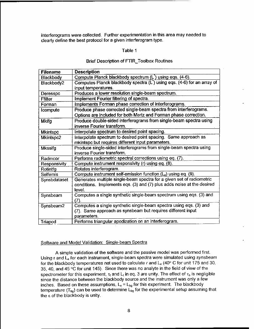
To correctly implement the nine steps for synthetic spectral generation listed above several MATLAB functions or "m-files" were written. Rather than just write several large programs that perform many functions, several smaller m-files were written to each perform a few limited tasks. These smaller routines form the basis for the larger ones. Table 1 outlines the routines and their uses. These m-files are incorporated into the "FTIRJToolbox", which the appendix describes in great detail. For the remainder of this report, the filename of the FTIRJToolbox routine being discussed will be denoted in the text with italics.

RESULTS AND DISCUSSION

Software and Model Validation: Instrument Responsivitv and Self-emission

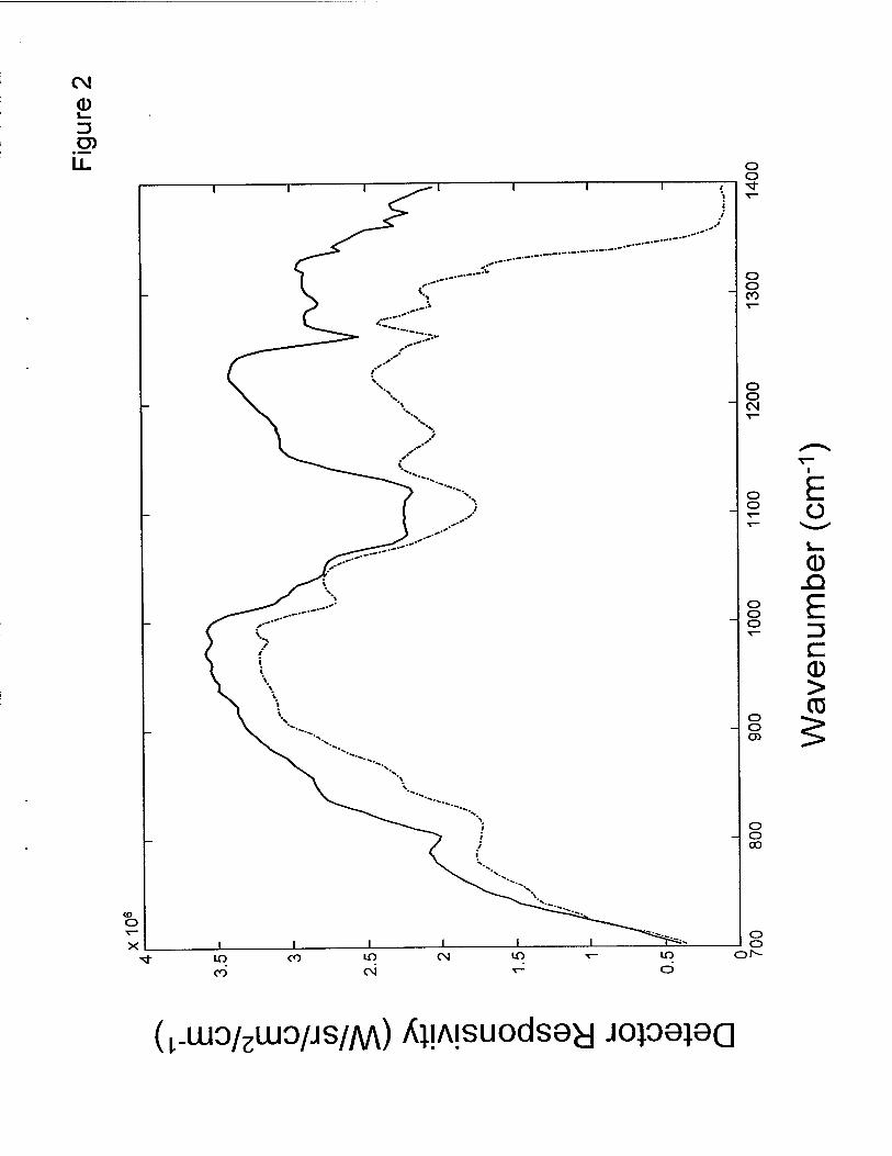
To validate the synthetic interferogram and single-beam spectral software and the passive IR models, several experiments were performed. Fifteen FT-IR interferograms were obtained from the two different Midac Outfielder emission spectrometers described in the experimental section. The blackbody temperatures for the interferograms from Midac Units 145 and 175 were (25, 30, 35, 40, 45, and 50 °C) and (30, 40, and 50 °C), respectively. TCA at a concentration of 1585 ppm-m and blank cell data were also collected on unit 175. For data processing, the interferograms were Mertz phase corrected and converted to single-beam spectra {icompute). Using responsivity and selfemis, the instrument responsivity and self-emission profiles were determined using the spectra collected at 25 and 50 °C for unit 145 and 30 and 50 °C for unit 175. These instrument specific functions are plotted in Figures 2 and 3. These figures illustrate the need for correcting l_x using eq. (7).

It should be noted that magnitude spectra are used in responsivity and selfemis. Revercomb et a/found that using complex spectra rather than just the magnitudes improved precision [30] using double-sided interferograms. Since the spectra that were used here were phase corrected prior to determining r and Le, the imaginary component of the complex spectrum was negligible. Further experimentation showed that, for the single-sided interferograms typically collected using passive FT-IR sensors, no accuracy is lost by phase correcting interferograms prior to the determination of r and Le. Most likely, improvements would only be seen for complex spectra when double-sided

ihterferograms were collected. Further experimentation in this area may needed to clearly define the best protocol for a given interferogram type.

Table 1

Brief Description of FTIR_Toolbox Routines

Filename Description Blackbody Compute Planck blackbody spectrum (L") using eqs. (4-6). Blackbody2 Computes Planck blackbody spectra (L") using eqs. (4-6) for an array of

input temperatures. Deresspc Produces a lower resolution single-beam spectrum. Ffilter Implement Fourier filtering of spectra. Forman Implements Forman phase correction of interferograms. Icompute Produce phase corrected single-beam spectra from interferograms.

Options are included for both Mertz and Forman phase correction. Mkifg Produce double-sided interferograms from single-beam spectra using

inverse Fourier transform. Mkintspc Interpolate spectrum to desired point spacing. Mkintspc2 Interpolate spectrum to desired point spacing. Same approach as

mkintspc but requires different input parameters. Mkssifg Produce single-sided interferograms from single-beam spectra using

inverse Fourier transform. Radmcor Performs radiometric spectral corrections using eq. (7). Responsivity Compute instrument responsivity (r) using eq. (8). Rotintfg Rotates interferogram. Selfemis Compute instrument self-emission function (U) using eq. (9). Synsbdataset Generates multiple single-beam spectra for a given set of radiometric

conditions. Implements eqs. (3) and (7) plus adds noise at the desired level.

Synsbeam Computes a single synthetic single-beam spectrum using eqs. (3) and (7).

Synsbeam2 Computes a single synthetic single-beam spectra using eqs. (3) and (7). Same approach as synsbeam but requires different input parameters.

Triapod Performs triangular apodization on an interferogram.

Software and Model Validation: Single-beam Spectra

A simple validation of the software and the passive model was performed first. Using r and U for each instrument, single-beam spectra were simulated using synsbeam for the blackbody temperatures not used to calculate r and Le (40° C for unit 175 and 30, 35, 40, and 45 °C for unit 145). Since there was no analyte in the field of view of the spectrometer for this experiment, it and Lt in eq. 3 are unity. The effect of xa is negligible since the distance between the blackbody source and the instrument was only a few inches. Based on these assumptions, Lx = Lbg for this experiment. The blackbody temperature (Tbg) can be used to determine Ug for the experimental setup assuming that the s of the blackbody is unity.

The predicted (or simulated) single-beam spectra for each unit and blackbody temperature were compared to the collected spectra. If the responsivity and self- emission profiles of the FT-IR are consistent during the experiments and the model is valid, there should be little difference between the predicted and actual (measured) spectra. Figure 4A shows the simulated single-beam spectra for unit 175 at 40°C. The relative difference (i.e., [(predicted-measured) / measured] x 100) between the simulated and actual single-beam spectra is shown in Figure 4B. Figure 5A contains simulated single-beam spectra for unit 145 at 30, 35, 40, and 45 °C. As expected based on eqs. (1) and (3), the single-beam spectral intensities are directly related to the temperature of the blackbody source. The relative difference between the simulated and actual single- beam spectra for unit 145 are shown in Figure 5B. Similar to Figure 4B, there is excellent agreement between the predicted and the actual spectra (errors < 1% in the 750-1300 cm"1 region). Inspection of Figure 5B indicates that there was probably a slight temperature drift of the instrument during the course of the experiments. The larger difference corresponds to the blackbody measurement at 25 °C, while the smallest difference was found at 45 °C. Internal temperature changes directly affect the r and U profiles of the instrument [29,31]. In fact, it has been shown that it is possible to linearly model r as a function of the internal temperature. Thus, any differences between the measured and predicted single-beam spectra are due to an inaccurate determination of r or U and not caused by the radiometric model. The positive residuals seen in Figures 4B and 5B indicate cases when the instrument was slightly warmer than the estimated r suggests, while negative residuals imply a slightly colder instrument than expected.

Software and Model Validation: Sinale-beam Spectra With Analvte Present

A more challenging test is to simulate a single-beam spectrum in which an analyte vapor is present in the field of view of the spectrometer. The steps are the same as above except tt and Lt must be incorporated into the analysis (i.e., used as inputs to synsbeam). The absorption coefficients for the target analyte (TCA) were downloaded from the AEDC/EPA website [21]. The concentration of TCA in the library spectrum was 504 ppm-m. The TCA absorbance spectrum is shown in Figure 6 for the 700-1400 cm"1

atmospheric window after deresolution and interpolation to 4 cm*1 point spacing. Interferograms of TCA in the gas cell were collected at three blackbody temperatures on unit 175. The instrument r and U were computed using single-beam spectra from the empty cell at 30 and 50°C. For the 40 °C blackbody measurement, the gas cell was filled with TCA at 1585 ppm-m. Prior to simulation, the TCA library spectrum was scaled by multiplying each point by 3.145 (1585/504 = 3.145). The temperature of the gas inside the cell was 22.9 °C (Tt) The effect of xa is negligible similar to the no analyte case discussed above.

The FTIR_Toolbox routine synsbeam was used to predict the single-beam spectrum of 1585 ppm-m TCA at 23.3°C with a background temperature of 40°C. Since the background temperature is hotter than the gas temperature, infrared absorbance is observed (i.e., a dip in the single-beam spectra where the analyte absorbs infrared energy). Figure 7A is the predicted single-beam spectrum of TCA. To highlight the analyte absorbance bands, the predicted background spectrum (same background temperature but no analyte) is superimposed. The difficulty in discerning the analyte bands are due to a combination of low concentration, insufficient temperature differential for background and the vapor, and the broadness of the band contour. The difference between the predicted and collected single-beam spectrum is shown in Figure 7B.

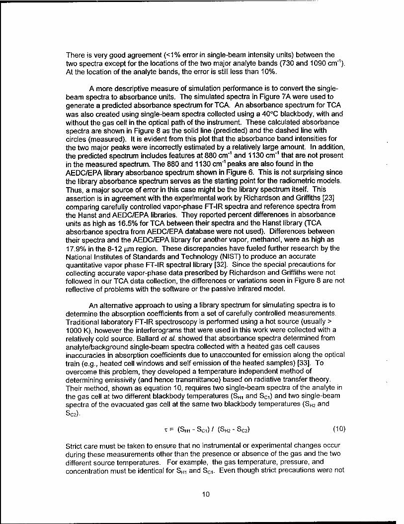
There is very good agreement (<1% error in single-beam intensity units) between the two spectra except for the locations of the two major analyte bands (730 and 1090 cm"1). At the location of the analyte bands, the error is still less than 10%.

A more descriptive measure of simulation performance is to convert the single- beam spectra to absorbance units. The simulated spectra in Figure 7A were used to generate a predicted absorbance spectrum for TCA. An absorbance spectrum for TCA was also created using single-beam spectra collected using a 40°C blackbody, with and without the gas cell in the optical path of the instrument. These calculated absorbance spectra are shown in Figure 8 as the solid line (predicted) and the dashed line with circles (measured). It is evident from this plot that the absorbance band intensities for the two major peaks were incorrectly estimated by a relatively large amount. In addition, the predicted spectrum includes features at 880 cm"1 and 1130 cm"1 that are not present in the measured spectrum. The 880 and 1130 cm"1 peaks are also found in the AEDC/EPA library absorbance spectrum shown in Figure 6. This is not surprising since the library absorbance spectrum serves as the starting point for the radiometric models. Thus, a major source of error in this case might be the library spectrum itself. This assertion is in agreement with the experimental work by Richardson and Griffiths [23] comparing carefully controlled vapor-phase FT-IR spectra and reference spectra from the Hanst and AEDC/EPA libraries. They reported percent differences in absorbance units as high as 16.5% for TCA between their spectra and the Hanst library (TCA absorbance spectra from AEDC/EPA database were not used). Differences between their spectra and the AEDC/EPA library for another vapor, methanol, were as high as 17.9% in the 8-12 urn region. These discrepancies have fueled further research by the National Institutes of Standards and Technology (NIST) to produce an accurate quantitative vapor phase FT-IR spectral library [32]. Since the special precautions for collecting accurate vapor-phase data prescribed by Richardson and Griffiths were not followed in our TCA data collection, the differences or variations seen in Figure 8 are not reflective of problems with the software or the passive infrared model.

An alternative approach to using a library spectrum for simulating spectra is to determine the absorption coefficients from a set of carefully controlled measurements. Traditional laboratory FT-IR spectroscopy is performed using a hot source (usually > 1000 K), however the interferograms that were used in this work were collected with a relatively cold source. Ballard et al. showed that absorbance spectra determined from analyte/background single-beam spectra collected with a heated gas cell causes inaccuracies in absorption coefficients due to unaccounted for emission along the optical train (e.g., heated cell windows and self emission of the heated samples) [33]. To overcome this problem, they developed a temperature independent method of determining emissivity (and hence transmittance) based on radiative transfer theory. Their method, shown as equation 10, requires two single-beam spectra of the analyte in the gas cell at two different blackbody temperatures (SHi and SCi) and two single-beam spectra of the evacuated gas cell at the same two blackbody temperatures (SH2 and Sc2)-

T= (SHI-SCI)/ (SH2-SC2) (10)

Strict care must be taken to ensure that no instrumental or experimental changes occur during these measurements other than the presence or absence of the gas and the two different source temperatures. For example, the gas temperature, pressure, and concentration must be identical for Sm and SCi. Even though strict precautions were not

10

taken during these experiments, it is worthwhile to determine TCA transmittance using eq (10) using data collected on unit 175.

For this calculation, the single-beam spectra collected from the blackbody at 50°C and 30°C were used. After conversion to absorbance, single-beam spectra were simulated for the case where a 40°C blackbody and gas cell filled with 1585 ppm-m TCA at 23.3°C was in the optical path of the spectrometer. Figure 8 shows the predicted absorbance spectrum (solid line with squares) using this methodology. It is quite clear from this plot that spectra simulated using an absorbance spectrum computed using Ballard's method are better than those simulated using a library absorbance spectrum. The two anomalous features at 880 cm"1 and 1130 cm"1 that are present in the library spectra do not appear in this simulated data. These two anomalous spectral features are identified as 1,4 dioxane and may be spectrally removed by its associated library reference spectra [21]. TCA at 97% purity is stabilized with 3% of 1,4 dioxane which is undoubtedly responsible for the contaminant peaks at 800 cm"1 and 1130 cm"1 [34]. Although the peak heights are still off by about 20%, the band contours are much more consistent with the measured spectrum. For many applications that are envisioned for synthetically generated spectra and interferograms, quantitative error levels of approximately 20% are adequate. It is quite evident from these experiments, that accurate estimation of the "true" absorbance for a given compound is critical to generating quantitative simulated spectra.

To see how the interferograms are affected by the slight errors at the band strengths and to further test the software, the predicted single-beam spectrum of TCA used to generate the absorbance spectrum in Figure 8 was transformed back to the time-domain (interferogram) using mkssifg. Figure 9A shows the 50 points before and after the centerburst (ZPD) of that interferogram (line with circles). Superimposed is the measured TCA interferogram (line with squares) after Forman phase correction. Figure 9B is the difference between the predicted and actual interferograms for the 50 points before and after the centerburst. There appears to little difference between the two interferograms in the centerburst region; residual intensity errors are less than 10%. This result was not unexpected since the TCA spectral bands are fairly narrow. Thus, their time-domain representation is spread throughout the first two hundred points in the interferogram on either side of the centerburst. The centerburst region is dominated by broad spectral features such as the detector response envelope. Larger interferogram residual intensities can be found in the wings of the interferogram where the narrow width spectral features can be seen. These results illustrate that the simulated data will be useful for either spectral or interferogram-based research studies.

Deresolution of Absorbance Spectra

Since spectra from FT-IR library sources are often available only at high resolution (0.25 or 0.5 cm"1), it is sometimes necessary to create lower resolution spectra (2, 4, 8, or 16 cm"1) for research studies. In FT-IR spectroscopy, the resolution depends on the maximum retardation of the interferometer scan [35]. Thus, the preferred method of producing a low resolution spectrum is to simply truncate the interferogram (i.e., multiply by a boxcar function) to obtain the desired retardation. However, in many cases (e.g., ref. 36), the original interferograms are not available. Several commercially available programs (PLSJToolbox [37] and GRAMS [38]) have routines to perform this task on absorbance spectra. The FTIR_Toolbox contains the routine deresspc that implements several methods as well. One of the available options in deresspc is to

11

average the in-between points (GRAMS method). Another simple approach is to perform a cubic spline interpolation. For producing very low resolution spectra from high resolution spectra, these methods sometimes produce anomalous features in the spectra and are not always recommended. The methods used in the PLS_Toolbox (deresolv.m) and the AEDC/EPA deresolution program are to convolve the high resolution spectrum with an instrument function (boxcar, triangular, blackman, etc.). Another option available in deresspc convolves the absorbance spectrum with an instrument function through a Fourier filtering procedure followed by cubic spline interpolation (mkintspc) to ensure correct point spacing. The convolution based methods all seem to work a sufficient degree. Further experimentation may need to be done to determine if one method works consistently better than another.

Generation of Synthetic Data Sets

The two examples described above illustrate that the passive FT-IR radiometric models are valid and, with the FTIR_Toolbox software, single-beam infrared spectra and interferograms can be simulated. However, feasibility testing and fundamental signal processing research studies require more than just a single noise free interferogram or spectrum. The routine synsbdataset in the FTIRJToolbox can be used to generate a synthetic data set for given background and gas temperature ranges (to compute Lbg and Lt), analyte cl ranges, desired noise level, and a particular FT-IR instrument (r and U)- Similar to the above examples, xa and B are assumed to minimally impact the simulated data.

The software randomly selects the temperatures and concentrations from within the input ranges. This is analogous to outdoor experiments where the temperatures and analyte concentrations can change rapidly. By carefully controlling the radiometric conditions, challenging remote sensing scenarios can be simulated and will provide supplemental data sets for difficult to generate open-air experiments. Several examples of how simulated data sets can be used is given by Shaffer and Combs [36].

CONCLUSIONS

Radiometric models for passive FT-IR sensing have been derived. Information describing the analyte (concentration and temperature), background temperature (or radiance), and atmospheric transmittance, allows simulations of single-beam FT-IR spectra and interferograms with programs written in MATLAB. These simulated data have been shown to agree with laboratory collected passive FT-IR spectra and interferograms. Due to difficulties in obtaining very accurate absorption coefficients, the simulated data discussed here cannot be used as a replacement for laboratory collected data for building quantitative calibration models. However, the simulated data provides a means of modeling and explaining the results obtained from experimental data. The simulation approach also offers a fundamental research tool for validating and improving signal processing strategies in passive FT-IR remote sensing.

12

ACKNOWLEGEMENTS

We gratefully acknowledge Robert T. Kroutil (U.S. Army ERDEC) for his interest and support. Charles Chaffin (Aerosurvery Inc.) is thanked for sharing FT-IR spectra used in studying the deresolution methods. Gary Small (Ohio University), Jean-Marc Theriault (DREV), and Bill Phillips (Arnold Air Force Base) are acknowledged for their helpful comments and suggestions. Andrew Szumlas (Ohio University) is thanked for collecting data from unit 175 used in this report. This research was supported by the U.S. Army ERDEC.

13

REFERENCES

1. D. F. Flanigan, "A Short History of Remote Sensing of Chemical Agents", Electro- Optical Technology for Remote Chemical Detection and Identification, M. Fallahi and E. Howden (Eds.), Vol. 2763, 2-17, (SPIE, Bellingham, WA, 1996).

2. D.F. Flanigan, "Detection of Organic Vapors with Active and Passive Sensors: A Comparison", Appl. Opt, 25 4253-4260 (1986).

3. J.T. Ditillo, R.L Gross, M.L.G. Althouse, W.M. Lagna, W.R. Loerop, and P.J. Deluca, "Lightweight Standoff Chemical Agent Detector", Optical Instrumentation for Gas Emissions Monitoring and Atmospheric Measurements, J. Leonelli, D.K. Killinger, W. Vaughan, M.G. Yost (Eds.), Vol. 2366, 166-173, (SPIE, Bellingham, WA, 1994).

4. T. Gruber, L. Grim, and J.T. Ditillo, "A Radiation Model for Passive Chemical Detection", Optical Instrumentation for Gas Emissions Monitoring and Atmospheric Measurements, J. Leonelli, D.K. Killinger, W. Vaughan, M.G. Yost (Eds.), Vol. 2366, 233-240, (SPIE, Bellingham, WA, 1994).

5. S.P. Levine and G.M. Russworm, "Fourier Transform Infrared Optical Remote Sensing for Monitoring Airborne Gas and Vapor Contaminants in the Field", Trends Anal. Chem., 13,258-262(1994).

6. W.G. Fately, R.M. Hammaker, M.D. Tucker, M.R. Witkowski, C.T. Chaffin, T.L. Marshall, M. Davies, M.J. Thomas, J. Arello, J.L. Hudson, and B.J. Fairless, "Observing Industrial Atmospheric Contaminants by FT-IR", Journal of Molecular Structure, 347, 153-168(1995).

7. R. Beer, Remote Sensing by Fourier Transform Infrared Spectrometry, (Wiley, New York, 1992).

8. G.W. Small, R.T. Kroutil, J.T. Ditillo, and W.R. Loerop, "Detection of Atmospheric Pollutants by Direct Analysis of Passive Fourier Transform Infrared Interferograms", Anal. Chem., 60, 264-269 (1988).

9. R.E. Shaffer, G.W. Small, R.J. Combs, R.B. Knapp, R.T. Kroutil, "Experimental Design Protocol for the Pattern Recognition Analysis of Bandpass Filtered Fourier Transform Infrared Interferograms", Chemom. Intell. Lab. Sys., 29, 89-108 (1995).

10. A.S. Bangalore, G.W. Small, R.J. Combs, R.B. Knapp, R.T. Kroutil, C.A. Traynor, and J.D. Ko, "Automated Detection of Trichloroethylene by Fourier Transform Infrared Remote Sensing Measurements", Anal. Chem., 69, 118-129 (1997).

11. M.J. Mattu and G.W. Small, "Quantitative Analysis of Bandpass-Filtered Fourier Transform Infrared Interferograms", Anal. Chem., 67, 2269-2278 (1995).

12. M.J. Mattu, G.W. Small, and M.A. Arnold, "Determination of Glucose in a Biological Matrix by Multivariate Analysis of Multiple Bandpass-Filtered Fourier Transform Near- Infrared Interferograms", Anal. Chem., 69, 4695-4702 (1997).

14

13. CT. Chaffin and T.L. Marshall, "Generating Well Characterized Chemical Plumes for Remote Sensing Research", Electro-Optical Technology for Remote Chemical Detection and Identification III, M. Fallahi and E. Howden (Eds.), Vol. 3383, 113-123, (SPIE, Bellingham, WA, 1998).

14. L. Grim, T. Gruber, and J.T. Ditillo, "Generation of Synthetic Remote FTIR Interferograms", Optical Instrumentation for Gas Emissions Monitoring and Atmospheric Measurements, J. Leonelli, D.K. Killinger, W. Vaughan, M.G. Yost (Eds.), Vol. 2366, 224-232, (SPIE, Bellingham, WA, 1994).

15. D.F. Flanigan, "Prediction of the Limits of Detection of Hazardous Vapors by Passive Infrared with the use of MODTRAN", Appl. Opt, 35, 6090-6098 (1996).

16. D.F. Flanigan, "Hazardous Cloud Imaging: A New Way of Using Passive Infrared", Appl. Opt, 36, 7027-7036 (1997).

17. M.L. Polak, J.L Hall, and K.C. Herr, "Passive Fourier-Transform Infrared Spectroscopy of Chemical Plumes: an Algorithm for Quantitative Interpretation and Real-Time Background Removal", Appl. Opt, 34, 5406-5412 (1995).

18. A. Hayden, E. Niple, and B. Boyce, "Determination of Trace-Gas Amounts in Plumes by the Use of Orthogonal Digital Filtering of Thermal-Emission Spectra", Appl. Opt, 35, 2802-2809 (1996).

19. F.W. Koehler and G.W. Small, "Calibration Transfer Results for Automated Detection of Acetone and Sulfur Hexafluoride by FTIR Remote Sensing Measurements", in Proceedings of the 1997 International Conference on Fourier Transform Spectroscopy, (American Institute of Physics, Woodbury, NY, 1997).

20. P.E. Field, R.J. Combs, and R.B. Knapp, "Equilibrium Vapor Cell for Quantitative IR Absorbance Measurements", Appl. Spectosc, 50,1307-1313 (1996).

21. Quantitative Infrared Vapor Phase Spectra, Contract #68D90055, U.S. Environmental Protection Agency, Emission Measurement Branch, Research Triangle Park, NC (1992); http://www.epa.gov/ttn/emc/ftir/welcome.html

22. W.L. Wolfe and G.J. Zissis, Infrared Handbook, (Office of Naval Research, 1982).

23. R.L. Richardson and P.R. Griffiths, "Evaluation of a System for Generating Quantitatively Accurate Vapor-Phase Infrared Reference Spectra", Appl. Spectrosc, 52, 143-153(1998).

24. P.L. Hanst and ST. Hanst, Infrared Spectra for Quantitative Analysis of Gases, Infrared Analysis, Inc., Potomac, MD (1992).

25. F.X. Kneizys, E.P. Shettle, L Abreu, J. Chetwynd, G. Anderson, W. Gallery, J. Selby, and S. Clough, Users Guide to LOWTRAN 7, AFGL-TR-88-0177, U.S. Air Force Geophysics Laboratory, Hanscom Air Force Base, MA (1988).

15

26. A. Berk, L.S. Bernstein, and D.C. Robertson, MODTRAN: A Moderate Resolution Model for LOWTRAN 7, GL-TR-89-1022, AD-A214-337, U.S. Air Force Geophysics Laboratory, Hanscom Air Force Base, MA (1989).

27. C.L. Wyatt, "CIRRIS-1A Interferometer: Radiometrie Analysis", Appl. Opt, 28, 5069- 5072(1989).

28. R. J. Combs, "Noise Assessment for Passive FT-IR Spectrometer Measurements",", in Electro-Optical Technology for Remote Chemical Detection and Identification III, M. Fallahi and E. Howden (Eds.), Vol. 3383, 75-91, (SPIE, Bellingham, WA, 1998).

29. J.A. Simonds, W.E. Costello, R.J. Combs, and R.T. Kroutil, "Internal Diagnostics for FT-IR Spectrometry", Electro-Optical Technology for Remote Chemical Detection and Identification II, M. Fallahi and E. Howden (Eds.), Vol. 3082,106-120, (SPIE, Bellingham, WA, 1997).

30. H.E. Revercomb, H. Buijs, H.B. Howell, D.D. Laporte, W.L. Smith, and LA. Sromovsky, "Radiometrie Calibration of IR Fourier Transform Spectrometers: Solution to a Program with the High Resolution Sounder", Appl. Opt, 27, 3210-3218 (1988).

31. A. Villemaire, M. Chamberland, J. Giroux, R.L Lachance, and J.M. Theriault, "Radiometrie Calibration of FT-IR Remote Sensing Instrumentation", Electro-Optical Technology for Remote Chemical Detection and Identification II, M. Fallahi and E. Howden (Eds.), Vol. 3082, 83-91, (SPIE, Bellingham, WA, 1997).

32. P.M. Chu, G.C. Rhoderick, D.V. Vlack, S.J. Wetzel, W.J. Lafferty, and F.R. Guenther, "A Quantitative Infrared Spectral Database of Hazardous Air Pollutants", Fresenius J. Anal. Chem., 360, 426-429 (1998).

33. J. Ballard, J.J. Remedios, and H.K. Roscoe, "The Effect of Sample Emission on Measurements of Spectral Parameters Using a Fourier Transform Absorption Spectrometer", J. Quant. Spectrosc. Radiat. Transfer, 48, 733-741 (1992).

34. Aldrich Chemical Catalog, Aldrich Chemical Co. Inc., Milwaukee, Wl, Catalog number T5, 470-4 [CAS # 72-55-6] page 1269, 1990-1991.

35. P.R. Griffiths and J.A. Dehaseth, Fourier Transform Infrared Spectrometry, (Wiley, New York, 1986).

36. R.E. Shaffer and R.J. Combs, "Signal Processing Strategies for Passive FT-IR Sensors", in Electro-Optical Technology for Remote Chemical Detection and Identification III, M. Fallahi and E. Howden (Eds.), Vol. 3383, 92-103, (SPIE, Bellingham, WA, 1998).

37. B.W. Wise and N.B. Gallagher, PLS Toolbox 2.0, (Eigenvector Technologies, Inc, Manson, WA, 1998).

38. GRAMS/32 Manual, (Galactic Industries, Salem, NH, 1998).

16

FIGURE CAPTIONS

Figure 1. Depiction of two passive FT-IR remote sensing measurement scenarios.

Figure 2. Instrument response function on the same scale for units 145 (solid line) and 175 (dashed line).

Figure 3. Instrument offset or self-emission function plotted on the same scale for units 145 (solid line) and 175 (dashed line).

Figure 4. Results of (A) generating a synthetic single-beam FT-IR spectrum for unit 175 and (B) relative residual intensity between measured and simulated spectra for unit 175.

Figure 5. Influence of source temperature on (A) simulated FT-IR single-beam synthetic spectra at 30°C (squares), 35°C (open circles), 40°C (+), and 45°C (solid line) for unit 145 and (B) the relative residual intensities between measured and simulated spectra at 30°C (squares), 35°C (open circles), 40°C (+), and 45°C (solid line) for unit 145.

Figure 6. Library TCA absorbance spectrum

Figure 7. Results of (A) generating a synthetic TCA FT-IR single-beam spectrum (solid line) with synthetic background spectrum (dashed line) superimposed and (B) calculating the residual intensity differences between simulated and measured TCA FT-IR single- beam spectra.

Figure 8. TCA FT-IR absorbance spectra computed from simulated spectra using a library TCA spectrum (solid line), simulated spectra using Ballard's method of determining analyte absorptivities (solid with squares), and measured spectra from unit 175 (dashed line with open circles).

Figure 9. Results from the simulation of FT-IR interferograms showing (A) the synthetic interferogram (open circles) and phase-corrected measured interferogram (solid squares) of TCA for the 50 points before and after the centerburst and (B) the residual intensities between the simulated and measured interferograms.

17

13

<D

I

0 c o

-4

cm

T3 C 13 O D)

Ü 03

-Q

03

CM <D 13 O)

E o

CD jQ

E C CD > CO

(kujo/2uuo/JS/AA) Ai!A|suods9y jopejea

CO

(D i_ 3 D)

E ^o

<D

E C CD > CÜ

(^UJO/^IUO/JS/AA) U0!SS!LU9-j|9S

LL

E L—

<D

E C

> so

(%) Äjisuajui lenpisay eAijeiay

(sjiun qje) Ajisuajui

o . o CO

o . o

O .O

E o

.o -£2 ? E

c > CO

o ■o

o ■ o

CO

o ■ o

(o/0) Äjjsuajui lenpjsey GAfleiay

(D

E Z3 C (D > (0

(sj|un qje) /tysuajui

CD

o o CO

o o CM

O O

O O o

E

0

E 13 c 0 > CO

o o

o o 00

o o

Goueqjosqv

13

E

<D

E c (D > CO

Ai!su8ju| |enpisay

o . o CO

o . o CM

O . O

E o

.8 | £ E

<D > 03

■8 £ CD

O O 0O

O CD

(sjiun qje) Ajjsuajui

00 <D ZJ O) o o

CO

o o CM

O o

o o o

E

(D .Q

E c CD > 05

o o

o o 00

o o

aoueqjosqv

D) LL

E

o

E (0 i—

2

Ajisuaiui lenpisay

(sjiun qje) /fysuajui

APPENDIX

This appendix contains the MATLAB source code ("m-file") for the functions that make up Version 1.0 of the FTIR_Toolbox. Please note that upon importing these m- files into a word processor, some line wrapping occurs which causes a single line of code to appear as two lines in the appendix. The input parameters for each m-file can be determined at the MATLAB prompt by typing help ftirjtoolbox. Electronic copies of these m-files as well as other useful routines for processing FT-IR interferograms and spectra can be obtained by contacting, Dr. Ronald E. Shaffer; Naval Research Laboratory; Chemistry Division; 4555 Overlook Ave, SW; Washington, DC 20375; email: shaffer@ccf.nrl.navy.mil; phone: 202-404-3361.

27

%FTIR_Toolbox, Version 1.0, Dec. 10, 1998 % %Ron Shaffer %Naval Research Laboratory %Chemistry Division %4555 Overlook Ave., SW %Washington, DC 20375 %email: shaffer@ccf.nrl.navy.mil %phone: 202-404-3361 % % %BLACKBODY: Generate a single theoretical blackbody frequency spectrum. %BLACKBODY2: Generate Blackbody frequency spectra for an array of temperatures %DERESSPC: Produces lower resolution spectrum %FFILTER: Implement Fourier Filtering %FORMAN: Performs forman phase correction on a matrix of interferograms %IC0MPUTE: Compute phase corrected spectra from interferograms %MKIFG: Make double-sided interferograms from spectra %MKINTSPC: Make an interpolated infrared spectrum using cubic splines %MKINTSPC2: Make an interpolated infrared spectrum using cubic splines %MKSSIFG: Make single-sided interferograms from spectra. %RADMCOR — Radiometrie spectral correction %RESPONSIVITY - Compute FT-IR instrument responsivity %ROTINTFG: Rotate interferogram so that %SELFEMIS — Compute FT-IR instrument self-emission %SYNSBDATASET — Compute synthetic single-beam data set %SYNSBEAM: Compute a synthetic single beam spectrum %SYNSBEAM2: Compute a synthetic single beam spectrum %TRIAPOD: Triangular apodization on an interferogram %[spec,f] = blackbody(temp,npts,resol); %[spec,f] = blackbody2(temp,npts,resol); %[newx,newy] = deresspc(oldx,oldy,rfac,rtype,ropt); %[out] = ffilter(raw,atype,ftype,params); %[fdmat,pifg] = forman(dmat,nppa); %[specmat,specx,phcalc,spec_unc,MaxFreq,pointspac] = icompute(ifgmat,pctype,samprate,npa); %[ifg] = mkifg(specy,specx); %[newx,newy] = mkintspc(oldx,oldy,finit,fend,fres); %[newx,newy] = mkintspc2(oldx,oldy,finit,fend,npts); %[ssifg] = mkssifg(specx, specy, nipts, ss); %[outspec] = radmcor(inspec, R,Le,opt); % [R, specx] = responsivity (sped, spec2, specl2x, Tl, T2,MaxFreq, npts, opt) ; %[output] = rotintfg(input); %(Le, specx) = selfemis (sped, spec2, specl2x, T1,T2,MaxFreq, npts) ; %[specx,specy,cone,Tt,Tb] = synsbdataset(absspcX,absspcY,absspcX2,absspcY2, minTt,maxTt,minTb,maxTb,SNR,R,Le,specxRLe,MaxFreq,npts,nspec,rngseed); % [specx, specy,Lt, Lb, Lx,R,Le] = synsbeam(absspcX,absspcY,Tt,Tb, sped, spec2, specl2x,Tl,T2,MaxFreq, npts) , %[specx,specy] = synsbeam2(absspcX,absspcY,Tt,Tb,R,Le,specxRLe,MaxFreq, npts); %[output,apdfunc] = triapod(input,atype)

28

function [spec,f] = blackbody(temp,npts,resol); % BLACKBODY: Generate a single theoretical blackbody frequency spectrum. % Unlike blackbody2 this routine operates on a single temperature at a time % and uses the resolution as the input rather than the number of points. % [spec] = blackbody(temp,npts,resol); % spec — output spectrum % f — frequency axis in wavenumbers % temp — temperature in Celsius % npts — desired number of points in spectrum % resol — spectral resolution in wavenumbers (i.e., 3.8574) % Author: Ron Shaffer, Naval Research Laboratory % Version: 1.0. 9/3/97 Original Version % 1.1. 11/6/97 changed to compute 0 response at 0 cm-1

% Constants cl = 1.191062 * 10"-12; c2 = 1.438786;

% Convert temperature from Celcius to Kelvin

temp = temp + 273.16;

% 0 cm-1 produces a value of 0 f(l) = 0; spec(l) = 0;

% Loop through desired spectral range.

for i = 2:npts

f(i) = (i-1) * resol; % current frequency in cm-1

spec(i) = (cl * (f(i)A3)) / (exp((c2 * f(i))/temp)-l);

end

29

function [spec,f] = blackbody2(temp,npts,resol); % BLACKB0DY2: Generate Blackbody frequency spectra for an array of temperatures % [spec] = blackbody2(temp,npts,resol); % spec — output spectrum % f — frequency axis in wavenumbers % temp — temperature in Celsius % npts — desired number of points in spectrum % resol — spectral resolution in wavenumbers (i.e., 3.8574) % Author: Ron Shaffer, Naval Research Laboratory % Version: 1.0. 9/3/97 Original Version % 1.1. 11/6/97 changed to compute response at 0 cm-1 % 2.0 12/22/97 Modified so that user could pass in multiple temperatures % and output a matrix of spectra

% Set Constants cl = 1.191062 * 10*-12; c2 = 1.438786; nspec = length(temp); spec = zeros(nspec,npts);

% Convert temperature from Celcius to Kelvin

temp = temp + 273.16;

% 0 cm-1 produces a value of 0 f(l) = 0;

% Loop through desired spectral range.

for i = 2:npts

f(i) = (i-1) * resol; % current frequency in cm-1

spec(:,i) = (cl * <f(i)*3)) ./ (exp((c2 * f(i))./temp)-1)';

end

30

function [newx,newy] = deresspc(oldx,oldy,rfac,rtype,ropt); % DERESSPC: Produces lower resolution spectrum % Equal point spacing of x is assumed. % [newx,newy] = deresspc(oldx,oldy,rfac,rtype,ropt); % Ron Shaffer — NRL — 5/1/98 Version 1.0 % 5/5/98 Version 1.1 Incorporate Fourier filtering % routines. % newx new x-axis in cm-1 % newy new y-axis in same units as oldy % oldx old x-axis in cm-1 % oldy old y-axis % rfac reduction factor (must be a power of 2) % rtype Type of reduction (1 = average in-between points, % 2=Fourier filtering with triangle apod.) % ropt Options for FF (fraction of zero-filling, first and last cm-1 in returned spectrum)

oldmaxx = max(oldx); oldminx = min(oldx); oldfres = (oldmaxx-oldminx)/(length(oldx)-1); fprintfCOld Spectrum: %8.4f - %8.4f cm-1, %8.4f spacing \n',oldminx,oldmaxx,oldfres) ;

if rtype == 1 % average in-between points fres = oldfres*rfac; newx = oldminx:fres:oldmaxx; fprintf('Target Spectrum: %8.4f - %8.4f cm-1, %8.4f spacing \n',oldminx,oldmaxx,fres); poi = 1:rfac:length(oldx); lastpoint = length(oldy); lastnewpoint = length(newx); % first and last points of new spectrum are special cases lastpoint = length(oldy); lastnewpoint = length(newx); newy(l) = mean(oldy(1:(rfac/2))); firstpos = lastpoint-(rfac/2)+1; newy(lastnewpoint) = mean(oldy(firstpos:lastpoint));

% remainder of points use the last rfac-1 and the next rfac points % to compute newy

for i = 2:(lastnewpoint-1) curoldx = poi(i); firstpos = curoldx-(rfac/2)+l; lastpos = curoldx+(rfac/2); newy(i) = mean(oldy(firstpos:lastpos));

end

end

if rtype == 2 % use Fourier filtering then interpolation

fres = oldfres*rfac; newx = ropt(2):fres:ropt(3); npts = length(newx); fprintf('Target Spectrum: %8.4f - %8.4f cm-1, %8.4f spacing \n',ropt(2),ropt(3),fres); [fout] = ffilter(oldy,0,3,ropt(D); (newx,newy] = mkintspc2(oldx,fout,ropt(2),ropt(3),npts);

end

31

function [out] = ffilter(raw,atype,ftype,params); % FFILTER: implement Fourier Filtering % [out] = ffilter(raw,atype,ftype,params); % out — filtered data % raw — input data % atype — type of apodization (0=boxcar (i.e., none), l=triangular, 2=bartlett, 3=blackman, % 4=hanning, 5=hamming, 6=kaiser-l, 7=kaiser-2) % ftype — filter function (l=boxcar, 2=Gaussian); % params — filter specific parameters % boxcar — [xboxon xboxoff] % e.g. [0 0.25] in % of total # of points in raw % Gaussian — [filter_position filter_width] % represented as a fraction of the total # of points in raw % Ron Shaffer — Naval Research Laboratory % Version 1.0 4/28/98 Original Code. % Based on filter in GRAMS/32 and ffil.f and GERM.f % written by Gary Small at Ohio university.

% Determine # of points in raw data npts = length(raw); orig_pnts = npts; % Apodize input data if necessary switch atype case 0

% no apodiation do nothing case 1

% triangular raw = raw .* triang(npts);

case 2 % Bartlett (page 4-2 in Signal Processing Toolbox Manual) raw = raw .* bartlett(npts);

case 3 % Blackman (generalized cosine) page 4-4 in Signal Proc. toolbox manual raw = raw .* blackman(npts);

case 4 % Hanning (page 4-4 in Signal Proc. toolbox manual) raw = raw . * hanning(npts);

case 5 % Hamming (page 4-4 in Signal Proc. toolbox manual) raw = raw .* hamming(npts);

case 6 % Kaiser 1 (page 4-5 in Signal Proc. toolbox manual) raw = raw .* kaiser(npts,1);

case 7 % Kaiser 3 raw = raw .* kaiser(npts,3);

case 8 % Kaiser 5 raw = raw .* kaiser(npts,5);

otherwise error ('ERROR: incorrect apodization function'),"

end

% If not a power of 2 pad with zeros test = rem(log2(npts) , 1); if test -= 1 % if not zero-fill to next power of 2

npts2 = pow2(nextpow2(npts)); raw(npts+l:npts2) = zeros(npts2-npts,1); npts = npts2; clear npts2;

end

% Forward FFT the raw data

craw = fft(raw); NumUniqPnts = ceil((npts+1)/2);

32

% Now Create Filter Function switch ftype case 1

%boxcar filter boxon = round)(params(1)*NumUniqPnts)+1); boxoff = round((params(2)*NumUniqPnts)); filtfunc = zeros(NumUniqPnts,1); filtfunc(boxon:boxoff) = boxcar(boxoff-boxon+1);

case 2 % Gaussian filter fpos = round((params(1)*NumOniqPnts) +1) ; fwid = params(2)*NumOniqPnts; filtfunc = gengauss(fwid,npts,fpos);

case 3 % Triangular filter triend = round(params(1)*NumUniqPnts); filtfunc = zeros(NumUniqPnts,1); i = 0:triend-l; filtfuncd:triend) = (triend - i)./triend;

otherwise error('ERROR: Improper Filter Function');

end % Multiply Filter Function and Complex Fourier Domain Data

craw2 = craw(l:NumUniqPnts) .* filtfunc;

% Reflect then Inverse Transform

craw2(NumUniqPnts+l:npts) = conj(flipud(craw2(2:NumUniqPnts-l))); out2 = real(ifft(craw2)); out = out2(1:orig_pnts) ;

33

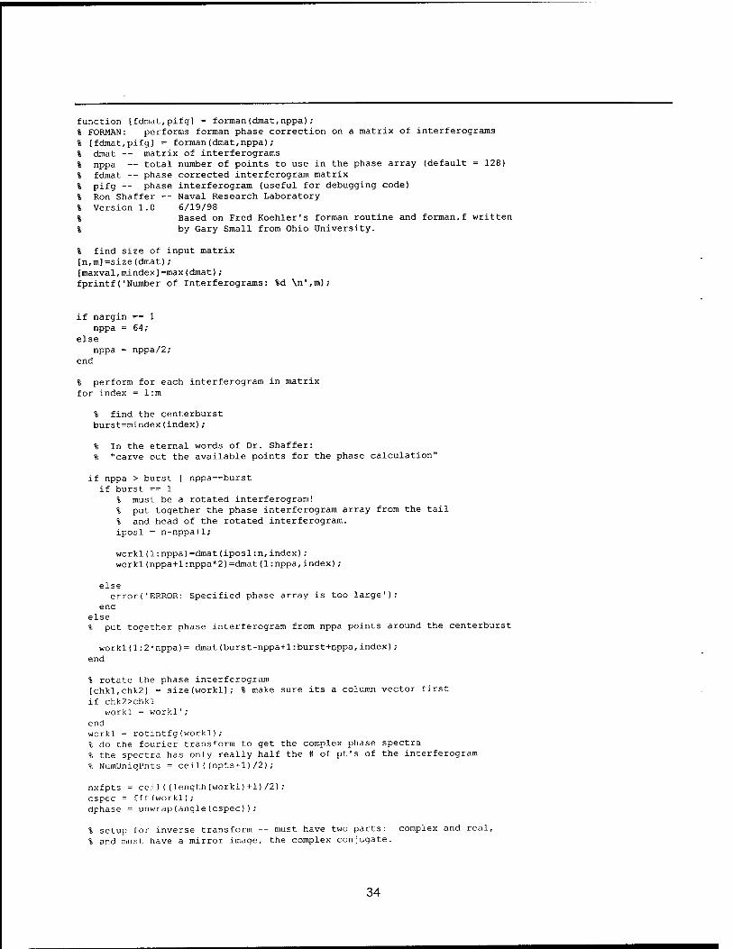
function [fdmat,pifg] = forman(dmat,nppa); % FORMAN: performs forman phase correction on a matrix of interferograms % [fdmat,pifg] = forman(dmat,nppa); % dmat — matrix of interferograms % nppa — total number of points to use in the phase array (default = 128) % fdmat — phase corrected interferogram matrix % pifg — phase interferogram (useful for debugging code) % Ron Shaffer — Naval Research Laboratory % Version 1.0 6/19/98 % Based on Fred Koehler's forman routine and forman.f written % by Gary Small from Ohio university.

% find size of input matrix [n,m]=size(dmat); [maxval,mindex]=max(dmat); fprintf('Number of Interferograms: %d \n',m);

if nargin == 1 nppa = 64;

else nppa = nppa/2;

end

% perform for each interferogram in matrix for index = l:m

% find the centerburst burst=mindex(index);

% In the eternal words of Dr. Shaffer: % "carve out the available points for the phase calculation"

if nppa > burst I nppa==burst if burst == 1

% must be a rotated interferogram! % put together the phase interferogram array from the tail % and head of the rotated interferogram. iposl = n-nppa+1;

workl(l:nppa)=dmat(iposl:n,index); workl(nppa+l:nppa*2)=dmat(1:nppa,index);

else error('ERROR: Specified phase array is too large');

end else % put together phase interferogram from nppa points around the centerburst

workl(l:2*nppa)= dmat(burst-nppa+1:burst+nppa,index); end

% rotate the phase interferogram [chkl,chk2] = size(workl); % make sure its a column vector first if chk2>chkl

workl = workl'; end workl = rotintfg(workl); % do the fourier transform to get the complex phase spectra % the spectra has only really half the # of pt's of the interferogram % NumUniqPnts = ceil((npts+1)/2);

nxfpts = ceil((length(workl)+1)/2); cspec = fft(workl); dphase = unwrap(angle(cspec));

% setup for inverse transform — must have two parts: complex and real, % and must have a mirror image, the complex conjugate.

34

rphase = cos(dphase)'; iphase = sin(dphase)'; cphase = (rphase - i*iphase);

% add the complex conjugate to the end.

nneg = nxfpts -1; tl = nxfpts+1; t2 = 2*nppa; cphase(tl:t2) = fliplr(conj(cphase(2:nneg)));

% Do the inverse fft from the complex phase spectrum to the real phase % interferogram.

intphase = ifft(cphase); pifg = intphase; intphase = real(intphase);

% reverse rotate (get centerburst into center for convolution) % and apodize the phase interferogram

phintfg = triapod(fftshift(intphase)');

% convolve input interferogram with phase interferogram

rintfg = conv(dmat(:,index),phintfg);

% fix after convolution screws up location of center burst, length. nout = n + nppa*2 -1; [rmax,nburst]=max(rintfg); iposl = nburst - burst +1; ipos2 = iposl+n-1; fdmat(l:n,index) = rintfg(iposl:ipos2);

end

35

function [specmat, specx, phcalc,spec_unc,MaxFreq,pointspac] = icompute(ifgmat,pctype,samprate,npa), % ICOMPUTE: compute phase corrected spectra from interferograms % [specmat,specx,phcalc,spec_unc] = icompute(ifgmat,pctype,samprate, npa); % specmat spectra (phase corrected if desired) % specx frequencies corresponding to spectral intensities in spec (i.e., the x-axis) % ifgmat input matrix of interferograms (npts,nspec) % pctype desired type of phase correction (l=mertz, 2=forman, 3 = none) % samprate — interferogram sampling rate (1 = every zero crossing, 2 every other, etc.) % This is used for compute the max. freq. in computed spectrum. % Assumes HeNe at 15798cm-l % npa desired number of points in phase array (optional)(default=256) % Ron Shaffer — Naval Research Laboratory % Version 1.0 4/24/98 % Original Code. Based loosely on cphase.f and pcspec.f by % Gary Small at Ohio University % % Version 1.1 4/27/98 % Check to make sure ifg is a power of 2 if not zero fill accordingly. % Fixed bug in selecting unique frequencies after FFT. See MATLAB Technical % Note #1702. % % Version 1.2 6/25/98 % Added capability to perform on multiple interferograms (i.e., a matrix) % % Version 1.3 8/18/98 % Added option for Forman phase correction of interferograms % % Version 1.4 11/25/98 % Added option for producing complex spectra with no phase correction

if (nargin==3) npa = 256; % default setting

end

[npts,nspec] = size(ifgmat);

if pctype == 1 for iter = l:nspec

ifg = ifgmat(:,iter); % check to see if ifg is a power of 2 test = rem(log2(npts),1); if test ~= 1 % if not zero-fill to next power of 2

npts2 = pow2(nextpow2(npts)); [maxval,cburstpos] = max(ifg); if cburstpos == 1

ifg = fftshift(ifg); % if centerburst is first rotate prior to zero filling end ifg(npts+l:npts2) = zeros(npts2-npts,nspec); npts = npts2; clear npts2;

end % search for centerburst (ZPD) [maxval,cburstpos] = max (ifg); % Carve out enough points around centerburst for the phase % calculation. If not enough points adjust accordingly. npa2 = npa/2; if (npa2) > cburstpos

istart = 1; ifin = 2*cburstpos; icbpnew = cburstpos; % cburstpos for small interferogram

else istart = cburstpos-npa2+l; ifin = cburstpos+npa2; icbpnew = npa2; % cburstpos for small interferogram

end work = ifg(istart:ifin); % apodize double-sided small interferogram work = triapod(work,2); % zerofill to the same # of points as the original interferogram

36

work(ifin:npts) = zeros((npts-ifin+1),1); % rotate interferogram work = rotintfg(work); % do the FFT cwork = fft(work); % compute phase array phcalc = unwrap(angle(cwork)); % % apodization, rotate, compute uncorrected spectrum. % nspecpnts = ceil((npts+1)/2); % See MATLAB Tech Note 1702 work2 = triapod(ifg,1); work2 = rotintfg(work2); spec_unc = fft(work2); % Determine Freq. ranges in spectra HeNe = 15798; %frequency of HeNe Laser in FT-IR MaxFreq = HeNe/samprate; specx = (0:nspecpnts-l) * 2 * MaxFreq/npts; % see MATLAB Tech Note 1702 % zero out points in phase array corresponding to locations where % phase is not defined (< 400 cm-1 and > 2000 cm-1 for most systems % that I use). This option is usually deselected. popt = 1; if popt — 2

boxcar = zeros(npts,1); jl = find(specx>400 & specxOOOO); boxcar(jl)=l; clear jl; phcalc = phcalc .* boxcar;

end % Mertz phase correct and return spec = (real(spec_unc(l:nspecpnts)) .* cos(phcalc(l:nspecpnts))) + (imag(spec_unc(l:nspecpnts))

.* sin(phcalc(1:nspecpnts))) ; specmat(:, iter) = spec;

end % end of Mertz phase correction and return

elseif pctype == 2 % must forman phase correction test = rem(log2(npts),1); for i = l:nspec

ifg = ifgmat(: ,i) ; if test -= 1 % if not zero-fill to next power of 2

[maxval,cburstpos] = max(ifg); if cburstpos == 1

ifg = fftshift(ifg); % if centerburst is first rotate prior to zero filling end npts2 = pow2(nextpow2(npts)); ifg(npts+l:npts2) = zeros(npts2-npts,1); npts = npts2; clear npts2;

end ifgmat2(:,i) = ifg;

end clear ifgmat; nspecpnts = ceil((npts+1)12); % See MATLAB Tech Note 1702 [fdmat) = forman(ifgmat2,npa); for i = l:nspec

ifg = fdmat(:,i) ; ifg = triapod(ifg,1); ifg = rotintfg(ifg); fdmat(:,i) = ifg;

end % Determine Freq. ranges in spectra

HeNe = 15798; %frequency of HeNe Laser in FT-IR MaxFreq = HeNe/samprate; specx = (0:nspecpnts-l) * 2 * MaxFreq/npts; % see MATLAB Tech Note 1702

work2 = fft(fdmat); specmat = real(work2(1:nspecpnts,:));

elseif pctype == 3 % no phase correction; produce complex spectrum test = rem(log2(npts),1);

37

for i'= l:nspec ifg = ifgmat(:,i); if test ~= 1 % if not zero-fill to next power of 2

[maxval,cburstpos] = max(ifg); if cburstpos == 1

ifg = fftshift(ifg); % if centerburst is first rotate prior to zero filling end npts2 = pow2(nextpow2(npts)); ifg(npts+l:npts2) = zeros(npts2-npts, 1); npts = npts2; clear npts2;

end ifgmat2(:,i) = ifg;

end clear ifgmat; nspecpnts = ceil((npts+1)/2); % See MATLAB Tech Note 1702 [fdmat] = ifgmat2; for i = l:nspec

ifg = fdmat(:,i); ifg = triapod(ifg,1); ifg = rotintfg(ifg); fdmat(:,i) = ifg;

end % Determine Freq. ranges in spectra

HeNe = 15798; %frequency of HeNe Laser in FT-IR MaxFreq = HeNe/samprate; specx = (0:nspecpnts-l) * 2 * MaxFreq/npts; % see MATLAB Tech Note 1702

work2 = fft(fdmat); specmat = (work2(1:nspecpnts,:));

end

38

function (ifg) = mkifg(specy,specx); % MKIFG: make double-sided interferograms from spectra % function [ifg] = mkifg(specy,specx); % ifg -- interferograms % specy — spectra % specx — frequency axis (default: assumes DC freq. not included) % Ron Shaffer — 5/1/97 — NRL % Version 1.1 — 12/8/98 — NRL % Make routine smart enough to % recognize when the input spectrum has % the zero'th frequency included.

% find length and number of spectra % assume rows are the number of spectra % and columns of the spectral points

if (nargin==l) specx(l) = 1; % default setting, DC frequency (0 cm-1)

% is not included in specy end

[nspec,npoints] = size(specy);

npoints2 = npoints*2; % create interferogram array

if specx(1) == 0 % is the DC freq included in the input spectra? % flip spectra specl = specy; spec2 = fliplr(specl); % complete spectra for processing spec3 = [specl'; spec2(:,2:(npoints-1))*]; % create interferogram arrays ifg = zeros(nspec,npoints2-2); % inverse FFT ifg = real(ifft(spec3))';

else % flip spectra specl = specy; spec2 = fliplr(specl); % complete spectra for processing spec3 = [zeros(l,nspec); specl'; spec2(:,2:npoints)']; % create interferogram arrays ifg = zeros(nspec,npoints2); % inverse FFT ifg = real(ifft(spec3))';

end

39

function [newx,newy] = mkintspc(oldx,oldy,finit,fend,fres); % MKINTSPC: Make an interpolated infrared spectrum using cubic splines % given an existing spectrum, This does the same calculation % as "mkintspc2" but requires different inputs. % Equal point spacing of x is assumed. % [newx,newy] = mkintspc(oldx,oldy,finit,fend,fres); % Ron Shaffer — NRL — 10/6/97 Version 1.0 % 7/30/98 fixed bug in computed oldfres % newx new x-axis in cm-1 % newy new y-axis in same units as oldy % oldx old x-axis in cm-1 % oldy old y-axis % oldres point spacing in oldx % finit starting cm-1 for interpolation % fend ending cm-1 for interpolation % fres desired point spacing in newx

oldmaxx = max(oldx); oldminx = min(oldx); oldfres = (oldmaxx-oldminx)/(length(oldx)-l) ; npts = round((abs(finit-fend))/fres); fprintfCOld Spectrum: %8.4f - %8.4f cm-1, %8.4f spacing \n',oldminx,oldmaxx,oldfres); fprintf('Target Spectrum: %8.4f - %8.4f cm-1, %8.4f spacing \n',finit,fend,fres); newx = finit:fres:fend; % now check to see if the old spectrum is % entirely within the range of the new spectrum. if oldmaxx < fend %fend is not within the range

templb = (min(find(newx>oldmaxx)))-l; %first location in newx where oldmmax ends temp_fend = newx(templb); tempi = npts-templb+1;

else temp_fend = fend; tempi = 0;

end if oldminx > finit

temp2b = max(find(newx<oldminx))+l;%first location in newx where oldminx begins temp_finit = newx(temp2b); temp2 = temp2b-l;

else temp_finit = finit; temp2 = 0;

end

xfinterp = temp_finit:fres:temp_fend; fprintf('Interpolating range %8.4f - %8.4f , %d # of points \n',min(xfinterp),max(xfinterp),length(xfinterp)); yfinterp = interpl(oldx,oldy,xfinterp,'spline');

fprintf('now adding %d points before and %d after interpolated spectrum for return \n',temp2,tempi) , % if tempi or temp2 = 1 then replace with closest value from orginal else % replace with zeros if (tempi == 1)

[jl,j2] = min(abs(oldx-temp_fend)); newy = [zeros(1, temp2) yfinterp oldy(j2)];

%elseif (temp2 == 1) % [jl,j2] = min(abs(oldx-temp_finit)) ; % newy = [oldy(j2) yfinterp zeros(1,tempi)]; else

newy = [zeros(1,temp2) yfinterp zeros(1,tempi)]; end

40

function [newx,newy] = mkintspc2(oldx,oldy,finit,fend,npts); % MKINTSPC2: Make an interpolated infrared spectrum using cubic splines % given an existing spectrum, This does the same calculation % as "mkintspc" but requires different inputs. % Equal point spacing of x is assumed. % [newx,newy] = mkintspc2(oldx,oldy,finit,fend,npts); % Ron Shaffer — NRL — 12/6/97 Version 1.0 % 5/1/98 Version 1.1 % fixed bug in calculating point spacing in oldx % newx new x-axis in cm-1 % newy new y-axis in same units as oldy % oldx old x-axis in cm-1 % oldy old y-axis % oldres point spacing in oldx % finit starting cm-1 for interpolation % fend ending cm-1 for interpolation % npts desired number of points in newx

oldmaxx = max(oldx); oldminx = min(oldx); oldfres = (oldmaxx-oldminx)/(length(oldx)-l); fres = (fend-finit) ./ (npts-1); fprintft'Old Spectrum: %8.4f - %8.4f cm-1, %8.4f spacing \n',oldminx,oldmaxx,oldfres); fprintf('Target Spectrum: %8.4f - %8.4f cm-1, %8.4f spacing \n',finit,fend,fres); newx = finit:fres:fend; % now check to see if the old spectrum is % entirely within the range of the new spectrum. if oldmaxx < fend %fend is not within the range

templb = (min(find(newx>oldmaxx)))-l; %first location in newx where oldmmax ends temp_fend = newx(templb); tempi = npts-templb;

else temp_fend = fend; tempi = 0;

end if oldminx > finit

temp2b = max(find(newx<oldminx))+l;%first location in newx where oldminx begins temp_finit = newx(temp2b); temp2 = temp2b-l;

else temp_finit = finit; temp2 = 0;

end

xfinterp = temp_finit:fres:temp_fend; fprintf('Interpolating range %8.4f - %8.4f , %d # of points \n',min(xfinterp),max(xfinterp),length(xfinterp)); yfinterp = interpl(oldx,oldy,xfinterp,'spline');

fprintf('now adding %d points before and %d after interpolated spectrum for return \n',temp2,tempi) , % if tempi or temp2 = 1 then replace with closest value from orginal else % replace with zeros if (tempi == 1) s (temp2 == 1)

[jl,j2] = min(abs(oldx-fend)); [J3,j4] = min(abs(oldx-finit)); newy = [oldy(j4) yfinterp oldy(j2)];

elseif (tempi == 1) [jl,j2] = min(abs(oldx-fend)); newy = [zeros(1,temp2) yfinterp oldy(j2)];

elseif (temp2 == 1) [jl,j2] = min(abs(oldx-finit)); newy = [oldy(j2) yfinterp zeros(1,tempi)];

else newy = [zeros(1,temp2) yfinterp zeros(1,tempi)];

end

41

function [ssifg] = mkssifg(specx, specy, nipts, ss); % MKSSIFG: make single-sided interferograms from spectra. % The spectrum must have greater than or equal the number % of points in the desired interferogram. (e.g., need 512 % spectral points to generate a 512 point single-sided interferogram). % function [ifg] = mkssifg(specx, specy, nipts, ss); % ssifg -- single-sided interferograms % nipts — number of desired points in interferogram (e.g., 1024) % ss — length of single sided portion (e.g., 100) % specx — wavenumber axis of specy % specy — spectra % Ron Shaffer — Naval Research Laboratory — 12/8/98 % Version 1.0 adapted from mkifg.m version 1.1 %

% find length and number of spectra % assume rows are the number of spectra % and columns of the spectral points

[nspec,nspecpoints] = size(specy); npoints2 = nspecpoints*2;

if (nspecpoints <= nipts) error('desired interferogram size too large');

end

% create interferogram array

dsifg = zeros(nspec,npoints2); ssifg = zeros(nspec,nipts); % check to see if zero'th frequency has been % included in the array

if specx(1) == 0 % is the DC freq included in the input spectra: % flip spectra sped = specy; spec2 = fliplr (sped) ; % complete spectra for processing spec3 = [sped'; spec2(:,2:(nspecpoints-1))']; % create interferogram arrays dsifg = zeros(nspec,npoints2-2); ssifg = zeros(nspec,nipts); % inverse FFT dsifg = real(ifft(spec3))';

else % flip spectra sped = specy; spec2 = fliplr (sped) ; % complete spectra for processing spec3 = [zeros (1, nspec) ; sped'; spec2 (:, 2 : nspecpoints) ' ] ; % create interferogram arrays dsifg = zeros(nspec,npoints2); ssifg = zeros(nspec,nipts); % inverse FFT dsifg = real(ifft(spec3))';

end

% current interferogram is double sided % now make it single-sided

dsifg = fftshift(dsifg); % shift so ZPD is the middle of the array % % Process each interferogram individually for i = l:nspec

% search for centerburst (ZPD)

42

[maxval,cburstpos] = max(dsifg(i,:)); istart = cburstpos-ss; ifin = istart + nipts -1; ssifg(i,:) = dsifg(i,istart:ifin) * 2; % scaling needs to be done

end

43

function [outspec] = radmcor(inspec,R,Le,opt); % RADMCOR — Radiometrie spectral correction % NOTE: assumes that x-axis for inspec, R, and Le are the same. % [outspec] = radmcor(inspec,R,Le,opt); % Ron Shaffer — Naval Research Laboratory % — Version 1.0 8/12/98 Original code % — Version 1.1 12/10/98 Added second option % inspec — input spectrum to be operated on (row vector) % R — instrument responsivity % Le — instrument self-emission curve % outspec — corrected spectrum % opt opt = 1: input is single-beam spectrum and output is a spectrum

in radiometric units (W/sr/cm2/cm-l) (basically strips out instrument specific features)

opt = 2: input is a spectrum in radiometric units and the output is a single-beam spectrum (i.e., adds instrument specific features)

if opt == 1 outspec = (inspec./R) - Le;

else outspec = R .* (inspec + Le)

end

44

function [R,specx] = responsivity (sped,spec2,specl2x,Tl,T2,MaxFreq,npts,opt); % RESPONSIVITY - compute FT-IR instrument responsivity % [R,specx] = responsivity (sped, spec2,specl2x,Tl,T2,MaxFreq, npts, opt); % Ron Shaffer 7/30/98 Original code based on specdiag.m % 11/25/98 If complex spectra are used (specl,spec2) then % uses the responsivity calculation developed by % Revercomb et al. Applied Optics 1988, 27, 3210-3218. % or if opt = 1 is selected use the method described % in A. Villemaire, Jean-Marc Theriault, et al., SPIE, % Volume 3082, pages 83-91. % sped — blackbody spectrum at temperature Tl (row vector) % spec2 — blackbody spectrum at temperature T2 (row vector) % specl2x — x-axis for specl,spec2,speclv,spec2v (row vector) % Tl — blackbody temperature for sped % T2 — blackbody temperature for spec2 % MaxFreq — maximum frequency in cm-1 (e.g., 1974.5) % npts — number of spectral points to compute (e.g., 512) % R — instrument Responsivity % specx — point spacing (x-axis) of R % opt — if complex spectra are used (1 = return complex R, 0 return real R), default=0

interpflag = 0; % compute X-axis values for spectra Fres = MaxFreq / (npts-1); specx = 0:Fres:MaxFreq;

if (nargin==9) opt = 0; % default setting

end

% transpose input x-axis and spectra if necessary. [nl,n2] = size(specl2x); if nl > n2

specl2x = specl2x'; end [nl,n2] = size(specl); if nl > n2

sped = sped'; end [nl,n2] = size(spec2); if nl > n2

spec2 = spec2'; end clear nl n2

% Now check if specl2X is the same as our target x-axis % if not then interpolate if (length(specx) == length(specl2x))

if ((sum(specx-specl2x))>0) interpflag = 1;

else interpflag = 0;

end else

interpflag = 1; end

if interpflag == 1 [junk,temp] = mkintspc2 (specl2x, sped, 0,MaxFreq, npts) ; sped = temp; [junk,temp] = mkintspc2(specl2x,spec2,0,MaxFreq,npts);

spec2 = temp; end

% Compute instrument Responsivity (R)

BB1 = blackbody(Tl,npts,Fres); BB2 = blackbody(T2,npts,Fres);

if (isreal(specl) == 1)& (isreal(spec2) == 1)

45

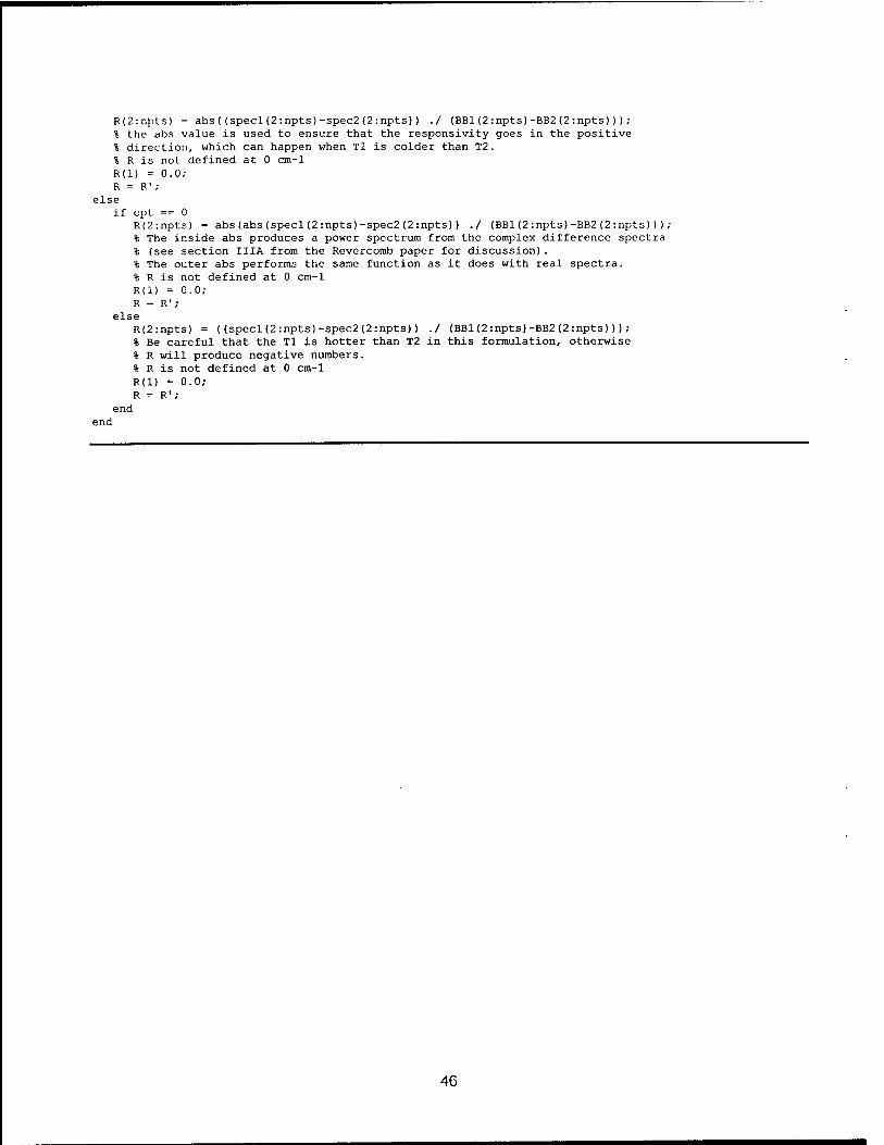
R(2:npts) = abs( (sped (2 :npts)-spec2 (2 :npts) ) ./ (BB1(2:npts)-BB2(2:npts))); % the abs value is used to ensure that the responsivity goes in the positive % direction, which can happen when Tl is colder than T2. % R is not defined at 0 cm-1 R(l) = 0.0; R = R';

else if opt == 0

R(2:npts) = abs (abs (sped (2 :npts) -spec2 (2:npts) ) ./ (BB1(2:npts)-BB2(2:npts))); % The inside abs produces a power spectrum from the complex difference spectra % (see section IIIA from the Revercomb paper for discussion). % The outer abs performs the same function as it does with real spectra. % R is not defined at 0 cm-1 R(l) = 0.0; R = R';

else R(2:npts) = ((specl(2:npts)-spec2(2:npts)) ./ (BB1(2:npts)-BB2(2:npts))); % Be careful that the Tl is hotter than T2 in this formulation, otherwise % R will produce negative numbers. % R is not defined at 0 cm-1 R(l) = 0.0; R = R';

end end

46

function (output] = rotintfg(input); % ROTINTFG: rotate interferogram so that % function [output] = rotintfg(input); % centerburst is at point #1 in the output array. % input unrotated interferogram % output rotated interferogram % Ron Shaffer Naval Research Laboratory % Version 1.0 9/18/97

% search for centerburst (ZPD) [maxval,cburstpos] = max(input);

% determine length of interferogram isize = max(size(input));

% now rotate inteferogram around centerburst position (cburstpos)

output = [input(cburstpos:isize)' input(1:(cburstpos-1))']' ;

47

function [Le,specx] = selfemis(specl,spec2,specl2x,Tl,T2,MaxFreq,npts), % SELFEMIS — compute FT-IR instrument self-emission function % [Le,specx] = selfemis(specl,spec2,specl2x,Tl,T2,MaxFreq,npts); % Ron Shaffer 7/30/98 Version 1.0 % specl — blackbody spectrum at temperature Tl (row vector) % spec2 — blackbody spectrum at temperature T2 (row vector) % specl2x — x-axis for specl,spec2,speclv,spec2v (row vector) % Tl — blackbody temperature for specl % T2 — blackbody temperature for spec2 % MaxFreq -- maximum frequency in cm-1 (e.g., 1974.5) % npts — number of spectral points to compute (e.g., 512) % Le — Instrument Self-emission % specx — point spacing (x-axis) of R and Le interpflag = 0; % compute X-axis values for spectra Fres = MaxFreq / (npts-1); specx = 0:Fres:MaxFreq; % transpose input x-axis and spectra if necessary. [nl,n2] = size(specl2x); if nl > n2

specl2x = specl2x'; end [nl,n2] = size(specl); if nl > n2

specl = specl'; end [nl,n2] = size(spec2); if nl > n2

spec2 = spec2'; end clear nl n2 % Now check if specl2X is the same as our target x-axis % if not then interpolate if (length(specx) == length(specl2x))

if ((sum(specx-specl2x))>0) interpflag = 1;

else interpflag = 0;

end else

interpflag = 1; end

if interpflag == 1 [junk,temp] = mkintspc2(specl2x,specl,0,MaxFreq,npts); specl = temp; [junk,temp] = mkintspc2(specl2x,spec2,0,MaxFreq,npts); spec2 = temp;

end

% Compute instrument Responsivity (R)

BB1 = blackbody(Tl,npts,Fres); BB2 = blackbody(T2,npts,Fres); Led) = 0; numerl = (specl(2:npts) .* BB2(2:npts)); numer2 = (spec2(2:npts) .* BB1(2:npts)); denom = spec2(2:npts) - specl (2:npts);

Le(2:npts) = (numerl-numer2)./denom;

% transpose and return

Le = Le';

48

function [specx,specy,cone,Tt,Tb] = synsbdataset(absspcX,absspcY,absspcX2,absspcY2,minTt,maxTt,minTb,maxTb,SNR,R,Le,specxRLe,MaxFreq,npts,ns pec,rngseed); % SYNSBDATASET — Compute synthetic single-beam data set % [specx,specy,cone,Tt,Tb] = synsbdataset(absspcX,absspcY,absspcX2,absspcY2,minTt,maxTt,minTb,maxTb, ... % SNR,R,Le,specxRLe,MaxFreq,npts,nspec,seed); % Ron Shaffer 12-21-97 Version 1.0 (based on synsbeam2.m) % 12-24-97 Version 1.1 (added Gaussian distributed random noise) % 1-20-98 Version 1.2 Fixed error in calculation of the % output single-beam spectra (specy = r*(Lx+Le)) % 1-29-98 Version 1.3 Add noise to Lx rather than final spectrum % specx — output synthetic single beam spectrum x-axis % specy — output synthetic single beam spectra y-axis % absspcX — absorbance spectrum for target analyte x-axis % absspcY — absorbance spectrum for target analyte y-axis % absspecX2 — absrorbance spectrum for interferent analyte x-axis % absspecY2 — absorbance spectrum for interferent analyte y-axis % minTt — Minimum temperature of target vapor cloud (in C) % maxTt — Maximum temperature of target vapor clound(in C) % minTb — Minimum temperature of background (in C) % maxTb — Maximum temperature of background (in C) % SNR — Target Signal-to-Noise ratio of the single-beam spectra % R — Instrument responsivity % specxRLe — x-axis for R and Le % Le — Instrument self-emission profile % MaxFreq — maximum frequency in cm-1 (e.g., 1974.5) % npts — number of spectral points to compute (e.g., 512) % nspec — number of single-beam spectra in each of the 4 classes (active, mix, intf, bkgd) % rngseed — seed # for random number generator

% initialize some parameters rngTb = maxTb - minTb; rngTt = maxTt - minTt; rand('state',rngseed)

% make sure the passed in spectra are column vectors (i.e., 512 X 1) tjl,j2] = size(specxRLe); if (jl < j2)

specxRLe = specxRLe'; end (jl,j2] = size(R); if (jl < j2)

R = R"; end [jl,j2] = size(Le); if (jl < j2)

Le = Le'; end [jl,j2J = size(absspcX); if (jl < j2)

absspcX = absspcX'; end

[jl,j2] = size(absspcY); if (jl < j2)

absspcY = absspcY'; end [jl,j2] = size(absspcX2); if (jl < j2)

absspcX2 = absspcX2'; end

[jl,j2] = size(absspcY2); if (jl < j2)

absspcY2 = absspcY2'; end

% interpolate target and interferent absorbance spectra to desired spectral range

49

Fres = MaxFreq / (npts-1); fprintf('Interpolating Target Analyte Library Spectrum \n'); [specx,absspcY3] = mkintspc2(absspcX,absspcY,0,MaxFreq,npts); fprintf('Interpolating Interferent Library Spectrum \n'); [specx,absspcY4] = mkintspc2(absspcX2,absspcY2,0,MaxFreq,npts); [jl,j2] = size (specx); if (jl < j2)

specx = specx'; end

[jl,j2] = size(absspcY3); if (jl < j2)

absspcY3 = absspcY3'; end

[jl,j2] = size(absspcY4); if (jl < j2)

absspcY4 = absspcY4'; end

% Now check if specxRLe is the same as our target x-axis % if not then interpolate if (length(specx) ~= length(specxRLe))

fprintf('Interpolating R spectrum \n'); [junk,speclb] = mkintspc2(specxRLe,R,0,MaxFreq,npts); fprintf('Interpolating Le spectrum \n'); [ junk, spec2b] ■= mkintspc2 (specxRLe, Le, 0, MaxFreq, npts) ; R = speclb; Le = spec2b; clear speclb spec2b; % rearrange if necessary [jl,j2] = size(R); if (jl < j2)

R = R'; end [jl,j2] = size(Le); if (jl < j2)

Le = Le ' ; end

elseif ((sum(specx-specxRLe))>0) fprintf('Interpolating R spectrum \n'); [junk,speclb] = mkintspc2(specxRLe,R,0,MaxFreq, npts) ; fprintf('Interpolating Le spectrum \n'); [junk,spec2b] = mkintspc2(specxRLe,Le, 0,MaxFreq,npts); R = speclb; Le = spec2b; clear speclb spec2b; % rearrange if Lecessary if (jl < j2)

R = R' ; end [jl,j2] = size(Le); if (jl < j2)

Le = Le ' ; end

end

% now start to create spectral data set % Group 1 contains analyte active only

% Randomly select analyte concentration % as fraction of library concentration

concl = 0.1 .* unidrnd(10,nspec,1); % cone values 0.1, 0.2, ... 1.0 tl = absspcY3 * concl';

% convert spectra to transmittance spectra tspecy =10."(-tl); clear tl;

50

% randomly select cloud and background temperature Tbl = (rand(nspec,l) .* rngTb) + minTb; Ttl = (rand(nsped) .* rngTt) + minTt;

% now compute blackbody spectra for background and analyte [Lb] = blackbody2(Tbl',npts,Fres); [Lt] = blackbody2(Ttl*,npts,Fres);

% compute apparent radiance (Lx)

Lx = (tspecy .* Lb') + ((1 - tspecy) .* Lt');

% Rearrange spectra to make sure everything is a column vector [jl, j2] = size(Lx) ; if (jl < j2)

Lx = Lx'; end

[jl,j2] = size(specx); if (jl < j2)

specx = specx'; end

% Add noise meanspec = mean(Lx'); [signal,wavpos] = max(meanspec); Lx = Lx + (randn(npts,nspec).*(signal/SNR));

% Compute Single-beam spectrum (specy or Sx)

specyl = (R*ones(l,nspec)) .* (Lx + (Le * ones(l,nspec))); % end of group 1

%%%%%%%%%%%%%%%%%%%%%%%%%%%%%%%%%%%%%%%%%%%%%%%%%%%%%%%%%%%%%%%%%%% % Group 2 contains analyte active and % interferent mixtures %%%%%%%%%%%%%%%%%%%%%%%%%%%%%%%%%%%%%%%%%%%%%%%%%%%%%%%%%%%%%%%%%%%%%%

% Randomly select analyte and interferent concentrations % as fraction of library concentration

conc2a = 0.1 .* unidrnd(10,nspec,1); % cone values 0.1, 0.2, ... 1.0 conc2b = 0.1 .* unidrnd(10,nspec,1); % cone values 0.1, 0.2, ... 1.0 tl = absspcY3 * conc2a'; t2 = absspcY4 * conc2b',- t3 = tl + t2; % add analyte and interferent spectra together

% convert spectra to transmittance spectra tspecy = 10.^(-t3); clear tl t2 t3;

% randomly select cloud and background temperature Tb2 = (rand(nspec,l) .* rngTb) + minTb; Tt2 = (randlnspec,1) .* rngTt) + minTt;

% now compute blackbody spectra for background and analyte [Lb] = blackbody2(Tb2',npts,Fres); [Lt] = blackbody2(Tt2',npts,Fres);

% compute apparent radiance (Lx)

Lx = (tspecy .* Lb') + ((1 - tspecy) .* Lt');

% Rearrange spectra to make sure everything is a column vector [jl, j2] = size(Lx); if (jl < j2)

Lx = Lx'; end

51

[jl,j2] = size(specx); if (jl < j2>

specx = specx'; end

% Add noise meanspec = mean(Lx'); [signal,wavpos] = max(meanspec); Lx = Lx + (randn(npts,nspec).*(signal/SNR));

% Compute Single-beam spectrum (specy or Sx)

specy2 = (R*ones(l,nspec)) .* (Lx + (Le * ones(l,nspec)));

%%%%%%%%%%%%%%%%%%%%%%%%%%%%%%%%%%%%%%%%%%%%%%%%%%%%%%%%%%%%%%%%%%%%« % Group 3 contains interferent spectra

% Randomly select interferent concentration % as fraction of library concentration

conc3 = 0.1 .* unidrnd(10,nspec,l); % cone values 0.1, 0.2, ... 1.0 tl = absspcY4 * conc3';

% convert spectra to transmittance spectra tspecy = 10."(-tl); clear tl;

% randomly select cloud and background temperature Tb3 = (rand(nspec,1) .* rngTb) + minTb; Tt3 = (rand(nspec,1) .* rngTt) + minTt;

% now compute blackbody spectra for background and analyte [Lb] = blackbody2(Tb3',npts,Fres); [Lt] = blackbody2(Tt3',npts,Fres);

% compute apparent radiance (Lx)

Lx = (tspecy .* Lb') + ((1 - tspecy) .* Lt');

% Rearrange spectra to make sure everything is a column vector [jl,j2] = size(Lx); if (jl < j2)

Lx = Lx'; end

[jl,j2] = size(specx); if (jl < j2)

specx = specx'; end

% Add noise meanspec = mean(Lx'); [signal,wavpos] = max(meanspec); Lx = Lx + (randn(npts,nspec).*(signal/SNR)) ;

% Compute Single-beam spectrum (specy or Sx)

specy3 = (R*ones(1,nspec)) .* (Lx + (Le * ones(1,nspec)));

%%%%%%%%%%%%%%%%%%%%%%%%%%%%%%%%%%%%%%%%%%%%%%%%%%%%%%%%%% % backgrounds

conc4 = zeros(nspec,1); tl = absspcY1! * conc4 ' ;

% convert spectra to transmittance spectra tspecy = 10."(-tl) ;

52

clear tl;

% randomly select cloud and background temperature Tb4 = (rand(nspec,l) .* rngTb) + minTb; Tt4 = (rand(nspecl) .* rngTt) + minTt;

% now compute blackbody spectra for background and analyte [Lb] = blackbody2(Tb4'(npts,Fres); [Lt] = blackbody2(Tt4',npts,Fres);

% compute apparent radiance (Lx)

Lx = (tspecy .* Lb') + ((1 - tspecy) .* Lt');

% Rearrange spectra to make sure everything is a column vector [jl,j2] = size(Lx); if (jl < j2)

Lx = Lx'; end

[jl,j2] = size(specx); if (jl < j2)

specx = specx'; end

% Add noise meanspec = mean(Lx'); [signal,wavpos] = max(meanspec); Lx = Lx + (randn(npts,nspec).*(signal/SNR));

% Compute Single-beam spectrum (specy or Sx)

specy4 = (R*ones(l,nspec)) .* (Lx + (Le * ones(l,nspec)));

specy = [specyl specy2 specy3 specy4]; % group spectra together

%%%%%%%%%%%%%%%%%%%%%%%%%%%%%%%%%%%%%%%%%%%%%%%%%%%% % return final data set of spectra cone = [concl conc2a conc2b conc3]; Tt = [Ttl Tt2 Tt3 Tt4]; Tb = [Tbl Tb2 Tb3 Tb4];

53

function [specx,specy, Lt, Lb,Lx,R,Le] = synsbeam(absspcX, absspcY, Tt,Tb, sped, spec2,specl2x,Tl,T2,MaxFreq, npts) ; % SYNSBEAM: compute synthetic single beam spectra % from absorbance spectra. This version also computes responsivity and self-emission. % [specx, specy, Lt, Lb, Lx,R, Le] = synsbeam(absspcX,absspcY,Tt,Tb, sped, spec2, spec 12x,Tl,T2,MaxFreq,npts) % Ron Shaffer 11-6-97 Version 1.0 % 1-20-97 Version 1.1 Fixed error in calculation of the % output single-beam spectrum (specy = r*(Lx+Le)) % 2-23-98 Added more error checking % 7-30-98 Added more error checking. To calculate a blackbody spectrum % (i.e., no analyte) absspcX must be an empty matrix []. absspcY and Tt are then % set to the appropriate default values % specx — output synthetic single beam spectrum x-axis % specy — output synthetic single beam spectrum y-axis % absspcX — absorbance spectrum for target analyte x-axis % absspcY — absorbance spectrum for target analyte y-axis % Tt — Temperature of target vapor cloud (in C) % Tb — Temperature of background (in C) % sped — blackbody spectrum at temperature Tl % spec2 — blackbody spectrum at temperature T2 % specl2x — x-axis for sped and spec2 % Tl — blackbody temperature for sped % T2 — blackbody temperature for spec2 % MaxFreq — maximum frequency in cm-1 (e.g., 1974.5) % npts — number of spectral points to compute (e.g., 512)

Fres = MaxFreq / (npts-1); specx = 0:Fres:MaxFreq;

if (isempty(absspcX) == 1) absspcX = specx; absspcY = zeros(1, npts); Tt = 0;

end

% more error checking to make sure that absspcx and absspcy are % row vectors (i.e., 513 rows x 1 column)

fjl,j2] = size(absspcX); if (jl>j2)

absspcX = absspcX'; end

[jl,j2] = size(absspcY); if (jl>j2)

absspcY = absspcY'; end

% interpolate absorbance spectrum to desired spectral range % if necessary

if (length(absspcX) ~= length(specx)) [specx,absspcY] = mkintspc(absspcX,absspcY,0,MaxFreq,Fres);

end

if sumfspecx - absspcX) > 0 [specx,absspcY] = mkintspc(absspcX,absspcY,0,MaxFreq, Fres) ,

end

% convert absorbance spectra to transmittance spectra

tspecy = 10. A (-absspcY) ,-

% now compute blackbody spectra for background and analyte [Lb] = blackbody(Tb,npts,Fres); [Lt] = blackbody(Tt,npts,Fres);

% compute apparent radiance (Lx)

54

Lx = (tspecy .* Lb) + ((1 - tspecy) .* Lt);

% Now check if specl2X is the same as our target x-axis % if not then interpolate

if length(specx) ~= length(specl2x) [junk,speclb] = mkintspc (specl2x, sped, 0,MaxFreq, Fres); [junk,spec2b] = mkintspc(specl2x,spec2,0,MaxFreq,Fres) ; sped = speclb; spec2 = spec2b; clear speclb spec2b;

elseif ((sum(specx-specl2x))>0) [junk,speclb] = mkintspc(specl2x,sped,0,MaxFreq,Fres) ; [junk,spec2b] = mkintspc(specl2x,spec2,0,MaxFreq,Fres); sped = speclb; spec2 = spec2b; clear speclb spec2b;

end

% more error checking to make sure that sped and spec2 are % row vectors (i.e., 513 rows x 1 column)

[jl,j2] = size(specl); if (jl>j2)

sped = sped'; end

[jl,j2] = size(spec2); if (jl>j2)

spec2 = spec2'; end

% Compute instrument Responsivity (R) and self-emission (Le)

[R] = responsivity(specl,spec2,specl2x,Tl,T2,MaxFreq,npts)'; [Le] = selfemis(specl,spec2,specl2x,Tl,T2,MaxFreq,npts)';

% Compute Single-beam spectrum (specy or Sx) and return

specy = R .* (Lx + Le);

55

function [specx,specy] = synsbeam2(absspcX,absspcY,Tt,Tb,R,Le,specxRLe,MaxFreq,npts); % SYNSBEAM2 — compute synthetic single beam spectra % from absorbance spectra. This version requires R and Le as inputs unlike "synsbeam"

[specx,specy Ron Shaffer

% % % % % % specx % specy % absspcX % absspcY % Tt % Tb % R % Le % specxRLe % MaxFreq % npts

synsbeam2(absspcX,absspcY,Tt,Tb,R,Le,specxRLe, MaxFreq, npts); Naval Research Laboratory

12-9-97 Version 1.0 1-20-97 Version 1.1 Fixed error in calculation of the output single-beam spectrum (specy = r*(Lx+Le))

7-30-98 Added more error checking. To calculate a blackbody spectrum (i.e., no analyte) absspcX must be an empty matrix []. absspcY and Tt are then set to the appropriate default values

— output synthetic single beam spectrum x-axis — output synthetic single beam spectrum y-axis — absorbance spectrum for target analyte x-axis — absorbance spectrum for target analyte y-axis — Temperature of target vapor cloud (in C)

— Temperature of background (in C) — Instrument responsivity

— Instrument self-emission profile — x-axis for R and Le — maximum frequency in cm-1 (e.g., 1974.5) — number of spectral points to compute (e.g., 512)

Fres = MaxFreq / (npts-1); specx = (0:Fres:MaxFreq)'; if (isempty(absspcX) == 1)

absspcX = specx; absspcY = zeros(npts,1); Tt = 0;

end

% make sure the passed in spectra are column vectors (i.e., 512 X 1) [jl,j2] = size(specxRLe); if (jl < j2)

specxRLe = specxRLe'; end [jl,j2] = size(R); if (jl < j2)

R = R'; end I jl,j2] = size(Le); if (jl < j2)

Le = Le'; end [jl,j2] = size(absspcX); if (jl < j2)

absspcX = absspcX'; end

[jl,j2] = size(absspcY); if (jl.< j2)

absspcY = absspcY'; end

% interpolate absorbance spectrum to desired spectral range % if necessary

if (length(absspcX) ~= length(specx)) [specx,absspcY] = mkintspc2(absspcX,absspcY,0,MaxFreq,npts); absspcY = absspcY';

elseif sum(specx - absspcX) > 0 [specx,absspcY] = mkintspc2(absspcX,absspcY,0,MaxFreq,npts); absspcY = absspcY';

end

% convert absorbance spectra to transmittance spectra

56

tspecy = lCM-absspcY);

% now compute blackbody spectra for background and analyte [Lb] = blackbody(Tb,npts,Fres)'; [Ltl = blackbody(Tt,npts,Fres)';

% compute apparent radiance (Lx) Lx = (tspecy .* Lb) + ((1 - tspecy) .* Lt);

% Rearrange spectra to make sure everything is a column vector [jl,j2] = size(Lx); if (jl < j2)

Lx = Lx"; end

[jl,j2] = size(specx); if (jl < j2)

specx = specx'; end

% Now check if specxRLe is the same as our target x-axis % if not then interpolate if (length(specx) ~= length(specxRLe))

(junk,speclb] = mkintspc2(specxRLe,R,0,MaxFreq,npts); [junk,spec2b] = mkintspc2(specxRLe,Le,0,MaxFreq,npts); R = speclb; Le = spec2b; clear speclb spec2b; % rearrange if necessary [jl,j2] = size(R); if (jl < j2)

R = R'; end [jl,j2] = size(Le); if (jl < j2)

Le = Le'; end

elseif ((sum(specx-specxRLe))>0) [junk,speclb] = mkintspc2(specxRLe,R,0,MaxFreq,npts); [junk,spec2b] = mkintspc2(specxRLe,Le,0,MaxFreq,npts); R = speclb; Le = spec2b; clear speclb spec2b; % rearrange if necessary if (jl < j2)

R = R'; end [ jl,j2] = size(Le); if (jl < j2)

Le = Le'; end

end

% Compute Single-beam spectrum (specy or Sx) specy = R .* (Lx + Le) ;

57

function [output,apdfunc] = triapod(input,atype) % TRIAPOD: Triangular apodization on an interferogram % output = triapod(input,atype) % atype is an optional parameter (see comments for version 1.1) % Ron Shaffer — Naval Research Laboratory % Version 1.0 4/17/98. Original Code — based on trapod.f by % Gary Small at Ohio University % Version 1.1 4/24/98. Incorporated code for trapod2.f by % Gary Small at Ohio university. When % atype == 1 weight apodization function ("left-ramp function" % of mostly single-sided interferogram to ensure % photometric accuracy (see page 31 and 32 of % Griffiths and DeHaseth, "Fourier Transform % Infrared Spectroscopy"). When atype == 2 % weigth points near centerburst equally. For % double-side and purely single-sided interferograms % atypel and atype2 are equivalent. atype==l is % the default setting. %

if (nargin==l) atype =1; % default setting

end

% search for centerburst (ZPD) [maxval,cburstpos] = max(input);

% determine length of interferogram

npts = length(input);

% initialize apodization function apdfunc = zeros(npts,1);

% First check to see whether this is a single or double % sided interferogram

fract = (min([cburstpos (npts-cburstpos)])) / npts;

if fract < 0.33 single_sided = 1;

else single_sided = 0;

end

% apodize up to centerburst. Handle case of single-sided % and double-sided differently if cburstpos > 1

if (single_sided == 1) & (atype == 1) firsthalf = 2*cburstpos-l; % see page 31, Griffeths and DeHaseth, 1986

else firsthalf = cburstpos;

end i = 1:firsthalf; apdfunc(l:firsthalf) = i./firsthalf;

else firsthalf = 1; % truely one-sided interferogram if cburstpos ==1 apdfunc(1) = 1;

end % now derive apodize function for backside secondhalf = npts-firsthalf; i = (firsthalf+1):npts; j = 1:secondhalf; apdfunc(i) = (npts-i)./secondhalf; % now multiply apodization function by original interferogram and return output = input .* apdfunc;

58