software effort estimation risk management over projects
TRANSCRIPT

Computer and Information Science; Vol. 11, No. 4; 2018 ISSN 1913-8989 E-ISSN 1913-8997
Published by Canadian Center of Science and Education
45
Software Effort Estimation Risk Management over Projects Portfolio Salma EL KOUTBI1 & Ali IDRI1
1 Software Project Management Research Team, Mohammed V University of Rabat, Rabat, Morocco Correspondence: Salma EL KOUTBI, Software Project Management Research Team, Mohammed V University of Rabat, ENSIAS BP 713 Agdal Rabat, Morocco. Tel: 212-661403143. E-mail: [email protected] Received: September 26, 2018 Accepted: October 9, 2018 Online Published: October 31, 2018 doi:10.5539/cis.v11n4p45 URL: https://doi.org/10.5539/cis.v11n4p45 Abstract Over the last decades, software development effort estimation has integrated new approaches dealing with uncertainty. However, effort estimates are still plagued with errors limiting their reliability. Thus, estimates error management at an organization level provides a promising alternative to the classical approaches dealing with single projects as a portfolio can afford more flexibility and opportunities in terms of risk management. The most widely used approaches in risk management were mainly based on the Gaussian approximation that shows its limits facing “ruin” risk associated to unusual events. The aim of this paper is to propose a Multi-Projects Error Modeling framework to characterize error at a portfolio level using bootstrapping, mixture of Gaussians and power law to emphasize the tail behavior respectively. Keywords: project management, project portfolio, risk management, software error estimation 1. Introduction 1.1 Introduce the Problem Software development effort estimation (SDEE) is a highly critical activity in software project management. Since estimating the effort required to develop a software project has a direct impact in costs control through the whole project lifecycle, the effort estimates can directly impact the project profitability leading to the project success or failure (Wen et al., 2012). SDEE has gained increasing attention and considerable researches and studies investigated numerous techniques in order to provide accurate estimates. In the systematic literature review (SLR) of software effort estimation studies performed between 2000 and 2004 conducted by (Jørgensen et al., 2007) 11 estimating techniques in 304 selected studies have been identified. In spite of all these efforts, the industry is still plagued with unreliable estimates. As effort estimation techniques did not success giving reliable estimates in all situations (Kitchenham et al. 1997), estimations always go hand in hand with risks (Patil 2007). Thus, estimates error assessment is a challenging and complex task as error sources are various and inherent to the effort estimation process. Kitchenham et al. (1997) have identified four different sources of error: (1) attributes measurement error that concerns the input variables; (2) model error that corresponds to the inherent limitation of a theoretical approach; (3) assumption error related to any inappropriate assumption made concerning the context and especially the model’s input parameters; and (4) scope error caused by the application of the model to a project outside the estimating domain. Furthermore, Kitchenham et al. (1997) suggest that managing error in SDEE should be investigated at an organizational level and not for a single project. In fact, a portfolio offers more possibilities in terms of risks management in comparison with a single project. In one hand, if a project had to ensure against all risks, the necessary staff and budget to protect aignst the worst case would be prohibitive. In the other hand, relying blindly on the lower value of estimated effort will lead organization to fatal consequences (Stamelos and Angelis 2001). This paper aims to explore Kitchemahm et al. (1997) assumption concerning error management at an organizational level for model error type. It consists of a primary step proposing a quantitative approach to model error at the portfolio level. This step is necessary in order to manage risks, since modeling a portfolio error provides the basis for risk analysis enabling designing the adapted risk buffers, as in finance and insurance. Our proposed Multi-Projects Error Modeling Framework (MPEM) relies on bootstrapping technique to increase

cis.ccsenet.org Computer and Information Science Vol. 11, No. 4; 2018
46
the number of estimates and tail events concept to better manage risk. In fact, to the best of author’s knowledge, the concept of tail events has not been investigated in combination with bootstrapping to deal with error in SDEE. Tail events correspond to unusual events with a very low probability of occurrence that can have a high impact on the portfolio profitability. In fact, tail events are associated with tail risks since they are so extreme and unexpected that they can cut deeply into the portfolio strategy (Taleb 2010). This idea took a high importance in 2008 after global markets nosedived and traumatized investors (Bhansali, 2008). Thus, the challenge was to figure out how to protect investments from extreme events causing massive losses. This interest was revving up again as revolutions in the Middle East and Japan's earthquake have destabilized markets and increased volatility (Bhansali, 2008). Nevertheless, bootstrapping has already been used in SDEE error management to increase the number of samples and estimates (El Koutbi et al., 2016). Especially: - Laqrichia et al. (2015) proposed a method based on bootstrapping to deal with uncertainty using neuronal networks based effort estimation. - Angelis and Stamelos (2000) improved the accuracy of Analogy-based effort estimation technique by means of bootstrapping. - Stamelos and Angelis (2001) investigated the concept of error over projects portfolio in order to manage errors over several projects by providing associated confidence intervals to point estimates over an interval. In this work, we use bootstrapping to explore the effort estimation technique behavior over different samples in order to provide a wide range of possible estimates. Based on the bootstrapped estimates, we propose an error handling framework consisting of two main steps: 1) a combination of two Gaussians is used to fit the body of error distribution, and 2) the power law distributions were used to approximate the right and left tails. This framework generates an error distribution which is more representative to model error and integrates the tail events. The main contributions of this study are to: (1) propose a framework to deal with error at an organization level whatever the estimation technique used, (2) integrate tail risk associated to tail events, and (3) evaluate the proposed framework using Analogy-based effort estimation technique over five datasets. To this end, we investigate the following research questions: (RQ1): Is there any evidence that model error management is more suitable at a portfolio level than at a single project level? (RQ2): Does the MPEM suits to the portfolio error over different datasets? (RQ3): Does the MPEM outperform the classical Gaussian approximation? This paper is organized as follow. Section 2 provides an overview of related works about error in SDEE while Section 3 gives insights into the Gaussian model, tail risk, mixture distribution and bootstrapping. Section 4 presents the MPEM framework dealing with model error at an organization level. Section 5 focuses on evaluation criteria and presents the experimental design of this study. Section 6 reports and discusses the results obtained. Section 7 underlines the threats of validity. Section 8 summarizes conclusions and future work. 2. Related Work In a systematic mapping study of dealing with error in SDEE, El Koutbi and al. (2016) analyzed 19 selected studies published between 1990 and 2015. The objective was to emphasize error approaches and classify them from six different viewpoints: research approaches, contribution types, accuracy criteria, datasets, error approaches and effort estimation techniques used. The main findings were the following: - There was a balance between studies proposing a managerial approach to error in SDEE and those developing a technique, framework or model to deal with error. - Over the studies proposing a technique, framework or model to deal with error in SDEE, 58% were for specific effort estimation techniques while 42% were adapted whatever the SDEE technique used. Both categories were new solutions proposal rather than improvements to existing approaches. - Most of the studies selected (89%) did not indicate which error types were investigated and none of the proposed techniques dealt with the four types of error sources. - No error technique was dominant. Still, the most used techniques were based on bootstrapping (11%) and fuzzy logic (16%). - 47% of selected studies used MRE (magnitude relative error) based accuracy criteria such as MMRE (mean of

cis.ccsenet.org Computer and Information Science Vol. 11, No. 4; 2018
47
MRE), MdMRE (median MRE) and Pred (Prediction Level), while only 21% of studies used confidence intervals. - Only one study (5% of selected studies) investigated error over more than one project and over a portfolio (Stamelos and Angelis 2001). Table 1 presents the findings of six selected studies as well as information including the effort estimation technique used, accuracy metrics and the error approach in each study especially for Stamelos’s approach of portfolio error management based on bootstrapping (Stamelos and Angelis 2001). Table 1. Literature overview of dealing with error in SDEE
Author (s) Proposed SDEE Error approach Accuracy metrics
Effort
estimation
technique
Findings/Methodology
Moataz Ahmed,
Zeeshan Muzaffar
A type-2 fuzzy logic based framework
handling both imprecision and
uncertainty in SDEE (Moataz et al.
2009)
RMSRE, Pred (25, 10) ML estimation
techniques
Use usually type-1 fuzzy logic to deal with imprecision. That shows promising results but has some limitations
since it cannot help managing uncertainty. The article investigates type-2 fuzzy logic and proposes a type-2 fuzzy
logic based framework to handle both imprecision and uncertainty. Evaluation experiments have shown interesting
results since the type-2 fuzzy framework outperforms the classical type-1 fuzzy approach.
Ioannis Stamelos,
Lefteris Angelis
Managing uncertainty over a portfolio
of projects (Stamelos and Angelis 2001)
Confidence intervals Analogy-based Propose to manage SDEE error at a portfolio level. In fact, software development organizations are usually involved
in more than one project simultaneously. Most of the approaches in SDEE concern single software projects. To
achieve the objective of project portfolio effort estimation error management, bootstrapping technique was used to
generate all the possible costs of a project portfolio.
Ali Idri, Taghi M.
Khoshgooftar,
Alain Abran
Integrating uncertainty and imprecision
in Case-Based Reasoning method for
Software Cost Estimation (Idri et al.,
2002)
Probability distribution Analogy-based Propose to integrate imprecision and uncertainty in the Analogy-based technique, since projects are described by vague
and imprecise attributes. As a result, instead of generating one single value, it becomes possible to generate a set of
possible values for the project effort. If needed, this set can be used to generate an end-point estimate.
Divya Kashyap, A.
K. Misra
Using Genetic Algorithm and fuzzy
numbers to deal with projects uncertainty
in SDEE (Kashyap and Misra, 2013)
MRE, MMRE Analogy-based
estimation
Deal with uncertainty associated with attributes measurement and data availability using fuzzy numbers in order to
improve the performance of SDEE. Furthermore, Genetic Algorithms help to derive the optimal effort adjustment.
The empirical evaluation shows that the obtained effort estimations were near to the actual efforts.
S.Laqrichia, F.
Marmiera,
D.Gourca, J.
Nevouxb
Integrating uncertainty in software effort
estimation using Bootstrap based Neural
Networks Laqrichia et al. (2015)
MMRE, Hit rate, Median Width,
Median ARPI
Neural
Networks
Use bootstrap resampling technique to improve the accuracy of a neural network based effort estimation technique. In
fact, taking into account uncertainty enables generating a probability distribution of effort estimates with a prediction
interval associated to a confidence level. The proposed empirical evaluation method has shown that the proposed
method outperformed traditional linear regression effort estimation.
Yeong-Seok Seo,
Kyung-A Yoon,
Doo-Hwan Bae
Using estimation error-based data
partitioning to improve the accuracy of
SDEE Multiple Least Square Regression
Models (Seo et al. 2009)
MMRE, MdMRE,
PredMRE(0.25), PredMRE(0.5),
MMER, MdMER,
PredMER(0.25), PredMER(0.5)
Least Square
Regression
Least Square Regression (LSR) is one of the well-known and widely used methods for SDEE estimation. Still, this
technique is largely affected by data distribution. Thus, this study considered the distribution of historical software
projects data as an important element impacting the effort estimation accuracy of a LSR model. It uses a data
partitioning method using the MRE and MER accuracy measures to improve effort estimation accuracy of LSR.
3. Background This section provides an overview of the main concepts and approaches explored in this paper. 3.1 Gaussian Model Gaussian distribution is a widely used continuous mathematical function characterized by a symmetric bell curve shape and used in many application fields (Feller, 1971 and Kenney et al., 1951). Thanks to the known central limit theorem, it takes an important place in statistics and probability (Spiegel, 1992 and Kraitchik, 1942). Indeed, under specific conditions, it corresponds to the behavior of series of similar and independent random experiments when the number of experiments is very important. This property makes it possible to approach other laws with normal distributions.In statistics, the Gaussian distribution describes normal distributions. In signal processing, it defines Gaussian filters to enhance signal quality. In image processing, two-dimensional Gaussians are used for Gaussian blurs. In mathematics, it helps solving heat and diffusion equations and to define the Weierstrass transform. In SDEE, it can model the effort estimation distribution as proposed by Kitchenham et al. (1997). The probability density of the Gaussian distribution is defined for 𝑥 ∈ ℝ as follows (Papoulis, 1984):
𝑓(𝑥|𝜎, 𝜇) = ( ) (1)
where μ is mean or expectation of the distribution, σ it standard deviation and 𝜎 is its variance. The Gaussian distribution can also be expressed with standard normal distribution:

cis.ccsenet.org Computer and Information Science Vol. 11, No. 4; 2018
48
𝑓(𝑥|𝜎, 𝜇) = 𝜙( ) (2)
where 𝜙 designates the standard normal distribution 𝜙(𝑥) = √
Historically, the Gaussian distribution appeared as the limit law in the central limit theorem using its cumulative distribution function. It is then useful to define its cumulative function. The cumulative distribution function of the standard normal distribution is usually denoted Φ and defined as: Φ(x) = √ 𝑒 𝑑𝑡 (3)
Figure 1, Gaussian distribution probability and cumulative function curves for 𝜇 = 0 𝑎𝑛𝑑 𝜎 = 1
3.2 Tail Risk Risk tail is a concept used in risk management, especially in financial markets. Since 2008, it took an important place in financial risk analysis especially after Wall Street global markets falls and panicked investors. The main issue was then to figure out how to protect investments from extreme events that cause massive losses (Vineer, 2008). The black swan metaphor was used by Taleb, to describe an event that comes as a surprise, has a major effect, and is often inappropriately rationalized after the event occurrence (Taleb 2010). In fact, the common technique used in finance to estimate the distribution of changes in price is a Gaussian approximation. This approach underestimates the values moving more than three times of standard deviations in comparison to the current price. Tail risk is then the risk of an asset or portfolio of assets moving more than times of standard deviations from its current price (Taleb, 2015). In reality, tails may be “fatter” than expected in traditional portfolio strategies relying on Gaussian bell curves to make market assumptions. Markets did not tend to behave “normally” since over the past three decades significant market collapses have occurred, resulting in “fatter” tails that a normal curve would predict. These unexpected collapses quickly spread panic across markets, creating a downward spiral of declines affecting a large spectrum of investments. Since they are so widespread and their magnitude so difficult to predict, tail events can have a devastating impact on portfolio returns corresponding to what is call “ruin” in insurance literature (Trevir, 2015). Figure 2 shows that the most probable returns, in a Gaussian bell curve, are concentrated in an interval near to the center, which is the average/mean expected return. The tails on the far left and far right represent the least likely and most extreme outcomes (i.e. lowest returns on the left and highest returns on the right). For long-term investors, the ideal portfolio strategy will seek to minimize left tail risk without curtailing right tail growth potential. In general, a tail risk is associated to an event with a small probability of happening. The term comes from looking at bell curve distributions. The tails of the bell curve extend out to plus or minus infinity with ever-decreasing probabilities. The associated probability of occurrence is small, if not tiny, in comparison with the “body” of the distribution. Still, the associated consequences of these events are extreme. Thus, it represents an important concern for risk management. In the rest of this paper, we use the following definitions (Taleb, 2015):
• Tail event is an event with small probability that takes place away from the center of the distribution. • Tail risk is associated to events that take place away from the center of the distribution. Tail risk is
crucial for risk management even if the body distribution takes generally more attention.

cis.ccsenet.org Computer and Information Science Vol. 11, No. 4; 2018
49
According to Robertson et al. (1969), the distribution of a random variable X is said to have a fat tail if: 𝑃(𝑋 > 𝑥)~𝑥 𝑎𝑠 𝑥 → ∞, 𝛼 > 0 (7) If 𝑋 has a probability density function 𝑓 (𝑥) 𝑓 (𝑥)~𝑥 ( ) 𝑎𝑠 𝑥 → ∞, 𝛼 > 0 (8) where ~ refers to the asymptotic equivalence and α is a positive index ∈ ℝ ∗.
Figure 2. Distribution of gain and losses in finance
Analysis of data and the reporting of the results of those analyses are fundamental aspects of the conduct of research. Accurate, unbiased, complete, and insightful reporting of the analytic treatment of data (be it quantitative or qualitative) must be a component of all research reports. Researchers in the field of psychology use numerous approaches to the analysis of data, and no one approach is uniformly preferred as long as the method is appropriate to the research questions being asked and the nature of the data collected. The methods used must support their analytic burdens, including robustness to violations of the assumptions that underlie them, and they must provide clear, unequivocal insights into the data. 3.3 Power Law Distributions Power law relations gained increasing attention over the last years and become an active topic of research in many fields including physics, computer science, linguistics, geophysics, neuroscience, sociology, and economics (Morrison and Schmittlein, 1980). In Mechanics, a power law relation can underline mechanisms that might emphasize an aspect of the explored phenomenon which indicate a deep connection with another. In instance, in physics, the ubiquity of power-law relations is partly due to dimensional constraints, while in complex systems, it is considered as the signature of hierarchy or some stochastic processes. In addition to that, much of the recent interest in power laws comes from the study of probability distributions. Indeed, the distributions of a wide variety of quantities seem to follow a power-law form, at least in their tail that corresponds to rare events. The behavior of these tail events corresponds particularly to stock market crashes and large natural disasters (Coles, 2001). A few notable examples of power laws are the Pareto's law of income distribution, scaling laws in biological systems and structural fractals self-similarity (Guerriero, 2012). A power law corresponds to a relation between two quantities that follows the form: 𝑓(𝑥) = 𝑎𝑥 (16) where 𝑎 ∈ ℝ and 𝛼 ∈ ℝ ∗. The power-law functional form can be considered as a special case of polynomial functions. Furthermore, for the general class of symmetric distributions with power law tails, the junction between the “body” and the “tail” of the distribution defines the domain of validity of the tail function. Formally, the tail starts at the crossover between “body” and “tail” that corresponds to (Taleb, 2015):
∓ ( )( )√ (17)
where 𝛼 is the stochastic volatility and 𝜎 the standard deviation. It worth notice that 𝛼 is infinite in the Gaussian

cis.ccsenet.org Computer and Information Science Vol. 11, No. 4; 2018
50
case. 3.4 Mixture Distributions Mixture distributions and mixture models are subjects of considerable interest in statistics. Mixture distributions represent a useful way of describing heterogeneity in the distribution of a variable, while mixture models provide a foundation for incorporating both deterministic and random predictor variables in regression models (Bruce, 1995). Mixture densities are generally complicated densities expressible in terms of simpler densities (the mixture components). They are used because they provide a good model for certain data sets especially when different subsets of the data exhibit different characteristics and can be modeled separately. In addition, the individual mixture components can be more mathematically tractable, because they can be more easily studied than the overall mixture density. Practically, mixture densities can be used to model a statistical population with subpopulations. The weights are the proportions of each subpopulation in the overall population and the mixture components are the densities on the subpopulations. It can also be used to model experimental error or contamination. Furthermore, in meta-analysis of separate studies, it enables studying heterogeneity causes distribution of results to be a mixture distribution (Frühwirth-Schnatter, 2006). The main idea behind mixture distributions is that the probability distribution of a random variable is derived from a collection of other random variables. In practice, the sample data observed is modeled as a random variable X that has some probability or weight wi of being drawn from distribution Di, for 𝑖 ∈ [1, 𝑛], where n is the number of components in the considered mixture distribution and ∑ 𝑤 = 1 . The key assumption is the statistical independence between the process of randomly selecting the component distribution Di and these distributions themselves. Formally, we define finite and countable mixtures as follows: For a finite set of probability density functions p , … , p and weights 𝑤 , … , 𝑤 with 𝑤 ≥ 0 and ∑ 𝑤 = 1, the mixture distribution can be represented by writing either the density f, or the distribution function F, as a sum: 𝐹(𝑥) = ∑ 𝑤 𝑃 (𝑥) (18)
𝑓(𝑥) = ∑ 𝑤 𝑝 (𝑥) (19) In the case of two distributions, we denote f the density associated with the distribution D1 and g the density associated with the distribution D2. Since the mixing percentages sum must be equal to 1, we denote w the weight associated to f and 1-w the weight associated to g. The overall probability density function p is then given by:
p(x) = w f(x) + (1 – w)g(x) (20) In the case where both f(x) and g(x) are Gaussian distributions, it is interesting to explore some of the possible results given in (Frühwirth-Schnatter, 2006; Robertson et al., 1969 and Behboodian, 1970). Figure 3 shows four specific examples. Figure 3.a shows the standard normal distribution (i.e., 𝜇 = 0 and 𝜎 =1), which corresponds to taking both f(x) and g(x) as standard normal densities, for any choice of w. It represents a reference case in interpreting the other distributions. Figure 3.b corresponds to the “contaminated normal outlier distribution”, widely used in the robust statistics literature. Since the measurement errors are traditionally modeled as zero-mean Gaussian random variables with a standard deviation 𝜎, the contaminated normal outlier distribution is mostly conform to this model; however a fraction (10% to 20%) of these measurement errors have larger variability. The traditional contaminated normal model defines w as the contamination percentage and assumes a standard deviation of 3𝜎 for these measurements. In Figure 3.b, w is equal to 0.15 (i.e., 15% contamination). Visually, Figure 3.b has a similar shape of Figure 3.a. Still, A Quantile-Quantile plot can easily show that the two distributions are not identical. Figure 3.c shows a two-components Gaussian mixture distribution where both components are equally represented (i.e., w = 0.5). The first component f(x) is the standard normal distribution and the second component g(x) is a Gaussian distribution with 𝜇 = 3 and standard deviation 𝜎 = 3 . The first component contributes the sharper main peak centered at zero, while the second component contributes the broad “shoulder” seen in the right half of the curve.

cis.ccsenet.org Computer and Information Science Vol. 11, No. 4; 2018
51
Figure 3.d corresponds to a mixture distribution with w = 0.40 where the first component is a Gaussian distribution with 𝜇 = −2 and 𝜎 = 1, and the second component is a Gaussian distribution with 𝜇 = +2 and 𝜎 = 1. The result is a bimodal distribution.
Figure 3. Mixture of Gaussian distributions 3.5 Bootstrapping Efron proposed the bootstrapping in 1979 when intensive computing calculations became affordable (Efron, 1979). This statistical technique refers to an inference approach that relies on random sampling with replacement. The concept of bootstrapping relies particularly on the idea that inference about a population from sample data can be modeled by resampling the sample data and performing inference about resampled data, knowing that the inference quality over the resampled data is measurable. Practically, it allows assigning measures of accuracy to sample estimates, especially in terms of confidence intervals (Efron et al., 1993). Two different modes of bootstrapping exist: parametric and non-parametric. The non-parametric bootstrap is based on the empirical distribution of the historical data set without any assumption on the population distribution. The parametric approach is based entirely on the assumption that the dataset comes from a theoretical distribution that has to be approximated by a parametric model. In practice, this can be a very complicated task as the statistical goodness-of-fit test for multivariate distributions are rare and hardly implemented. Additionally, some variables need to be transformed first causing some difficulties in the implementation and the usability of the method. Bootstrapping is widely used in statistical analysis in different fields of interest especially in finance, insurance, natural disasters prediction, biology (Efron et al., 1993). In SDEE, it is used in two different ways: (1) to improve the performance of effort estimation techniques (Angelis and Stamelos, 2000) or (2) to manage error at a portfolio level (Stamelos and Angelis 2001). In fact, since effort estimation techniques produced in general a single estimate, the bootstrap method helps calculating a confidence interval for a point estimate (Tukey, 1958). In practice, when dealing with a random sample of size n, this sample can provide single point estimation. In order to provide other estimates, we need several samples of the same size. Then, bootstrapping enables generating samples by replacements. That corresponds to the procedure where a random number generator selects integers i1, i2, … in between 1 and n with the probability 1/n. These integers determine which members of the original sample were selected to be in the new random sample. As a consequence of this approach, in every new sample, there are data points which appear more than once. 4. A New Framework MPEM to Portfolio Model Error Management Model error corresponds to the inherent error of the effort estimation technique. A SDEE model error is mainly due to: 1) a model is an abstraction of reality and it may therefore produce inaccurate estimates when it is evaluated in different contexts; and 2) a model cannot in general consider all the relevant cost drivers since it only used the available and known ones. Thus, this paper proposes a novel approach MPEM to better manage model error at a portfolio level. To do that, we use a mixture of Gaussian distributions in combination with the power law. Widely used in probability and statistics, Gaussian distribution has already been used in SDEE. In fact, El Koutbi
cis.ccsenet.org Computer and Information Science Vol. 11, No. 4; 2018
52
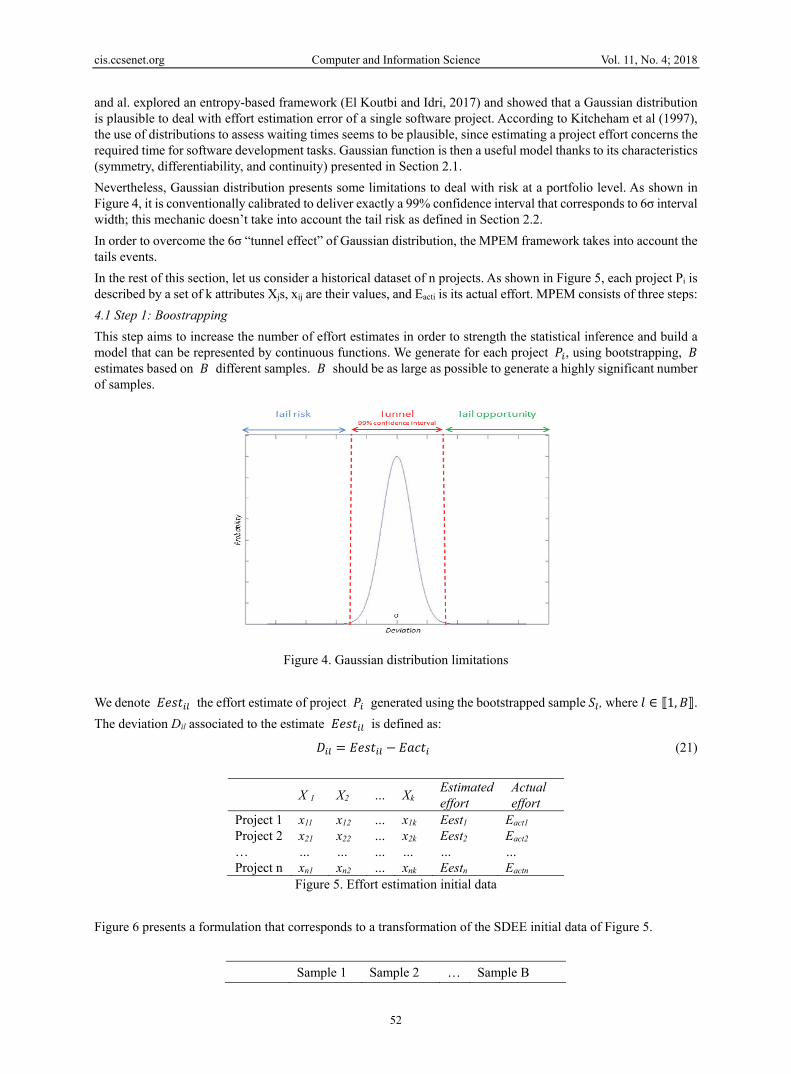
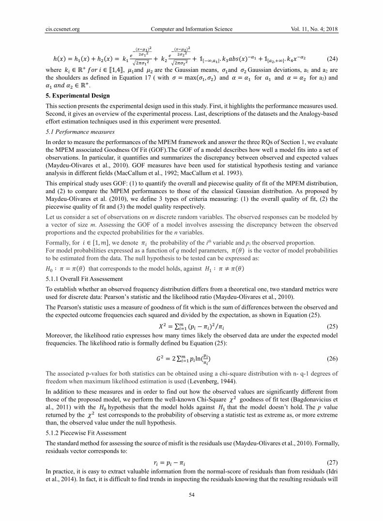
and al. explored an entropy-based framework (El Koutbi and Idri, 2017) and showed that a Gaussian distribution is plausible to deal with effort estimation error of a single software project. According to Kitcheham et al (1997), the use of distributions to assess waiting times seems to be plausible, since estimating a project effort concerns the required time for software development tasks. Gaussian function is then a useful model thanks to its characteristics (symmetry, differentiability, and continuity) presented in Section 2.1. Nevertheless, Gaussian distribution presents some limitations to deal with risk at a portfolio level. As shown in Figure 4, it is conventionally calibrated to deliver exactly a 99% confidence interval that corresponds to 6σ interval width; this mechanic doesn’t take into account the tail risk as defined in Section 2.2. In order to overcome the 6σ “tunnel effect” of Gaussian distribution, the MPEM framework takes into account the tails events. In the rest of this section, let us consider a historical dataset of n projects. As shown in Figure 5, each project Pi is described by a set of k attributes Xjs, xij are their values, and Eacti is its actual effort. MPEM consists of three steps: 4.1 Step 1: Boostrapping This step aims to increase the number of effort estimates in order to strength the statistical inference and build a model that can be represented by continuous functions. We generate for each project 𝑃 , using bootstrapping, 𝐵 estimates based on 𝐵 different samples. 𝐵 should be as large as possible to generate a highly significant number of samples.
Figure 4. Gaussian distribution limitations We denote 𝐸𝑒𝑠𝑡 the effort estimate of project 𝑃 generated using the bootstrapped sample 𝑆 , where 𝑙 ∈ ⟦1, 𝐵⟧. The deviation Dil associated to the estimate 𝐸𝑒𝑠𝑡 is defined as: 𝐷 = 𝐸𝑒𝑠𝑡 − 𝐸𝑎𝑐𝑡 (21)
X 1 X2 … Xk
Estimated effort
Actual effort
Project 1 x11 x12 … x1k Eest1 Eact1 Project 2 x21 x22 … x2k Eest2 Eact2 … … … … … … … Project n xn1 xn2 … xnk Eestn Eactn
Figure 5. Effort estimation initial data Figure 6 presents a formulation that corresponds to a transformation of the SDEE initial data of Figure 5.
Sample 1 Sample 2 … Sample B

cis.ccsenet.org Computer and Information Science Vol. 11, No. 4; 2018
53
Project 1 D11 D12 … D1B Project 2 D21 D22 … D2B … … … … … Project n Dn1 Dn2 … DnB Figure 6. Effort estimation formulation using bootstrapping
Based on the B samples, we generate the deviation distribution vector, denoted 𝐷, where 𝐷 ∈ ℝ . This vector contains all the computed deviations 𝐷 = 𝐷 , … , 𝐷 . 4.2 Step 2: Body distribution modeling The objective of this step is to approximate the generated bootstrapped deviations by the means of a mixture of two Gaussians following the scheme of a “contaminated normal outlier distribution” shown in Figure 3.b. This step enables to fit the “body” of the deviation distribution. Based on vector D, a first approximation of Equation (22) is used.
ℎ (𝑥) = 𝑘 ( ) + 𝑘 ( ) (22)
where 𝑘 ∈ ℝ 𝑓𝑜𝑟 𝑖 ∈ ⟦1,2⟧ are proportionate scaling factors, 𝜇 and 𝜇 are the Gaussian means and 𝜎 and 𝜎 Gaussian deviations.
Figure 7. MPEM error distribution
4.3 Step 3: Tails Distribution Modeling Step 3 focuses on tails and approximate them using power law functions. Based on Equation (17), we use the following formulation for tails modeling: ℎ (𝑥) = 𝟙[ , ]. 𝑘 𝑎𝑏𝑠(𝑥) + 𝟙[ , ]. 𝑘 𝑥 (23) where 𝛼 , 𝛼 ∈ ℝ , 𝑘 , 𝑘 ∈ ℝ and 𝑎 , 𝑎 ∈ ℝ Figure 7 shows the final shape of the MPEM distribution. The body corresponds to the mixture of two Gaussians. At the shoulders a1 and a2, the distribution corresponds to the superposition of the Gaussians dropping down and the power law functions. It is worth precise that the tails functions could be different resulting in a non-symmetric curve. Formally, the proposed density h associated to vector D is the following:
cis.ccsenet.org Computer and Information Science Vol. 11, No. 4; 2018
54
ℎ(𝑥) = ℎ (𝑥) + ℎ (𝑥) = 𝑘 ( ) + 𝑘 ( ) + 𝟙[ , ]. 𝑘 𝑎𝑏𝑠(𝑥) + 𝟙[ , ]. 𝑘 𝑥 (24)
where 𝑘 ∈ ℝ 𝑓𝑜𝑟 𝑖 ∈ ⟦1,4⟧, 𝜇 and 𝜇 are the Gaussian means, 𝜎 and 𝜎 Gaussian deviations, a1 and a2 are the shoulders as defined in Equation 17 ( with 𝜎 = max (𝜎 , 𝜎 ) and 𝛼 = 𝛼 for 𝑎 and 𝛼 = 𝛼 for a2) and 𝛼 𝑎𝑛𝑑 𝛼 ∈ ℝ . 5. Experimental Design This section presents the experimental design used in this study. First, it highlights the performance measures used. Second, it gives an overview of the experimental process. Last, descriptions of the datasets and the Analogy-based effort estimation techniques used in this experiment were presented. 5.1 Performance measures In order to measure the performances of the MPEM framework and answer the three RQs of Section 1, we evaluate the MPEM associated Goodness Of Fit (GOF).The GOF of a model describes how well a model fits into a set of observations. In particular, it quantifies and summarizes the discrepancy between observed and expected values (Maydeu-Olivares et al., 2010). GOF measures have been used for statistical hypothesis testing and variance analysis in different fields (MacCallum et al., 1992; MacCallum et al. 1993). This empirical study uses GOF: (1) to quantify the overall and piecewise quality of fit of the MPEM distribution, and (2) to compare the MPEM performances to those of the classical Gaussian distribution. As proposed by Maydeu-Olivares et al. (2010), we define 3 types of criteria measuring: (1) the overall quality of fit, (2) the piecewise quality of fit and (3) the model quality respectively. Let us consider a set of observations on m discrete random variables. The observed responses can be modeled by a vector of size m. Assessing the GOF of a model involves assessing the discrepancy between the observed proportions and the expected probabilities for the n variables. Formally, for 𝑖 ∈ [1, 𝑚], we denote 𝜋 the probability of the ith variable and pi the observed proportion. For model probabilities expressed as a function of q model parameters, 𝜋(𝜃) is the vector of model probabilities to be estimated from the data. The null hypothesis to be tested can be expressed as: 𝐻 ∶ 𝜋 = 𝜋(𝜃) that corresponds to the model holds, against 𝐻 ∶ 𝜋 ≠ 𝜋(𝜃) 5.1.1 Overall Fit Assessement To establish whether an observed frequency distribution differs from a theoretical one, two standard metrics were used for discrete data: Pearson’s statistic and the likelihood ratio (Maydeu-Olivares et al., 2010). The Pearson's statistic uses a measure of goodness of fit which is the sum of differences between the observed and the expected outcome frequencies each squared and divided by the expectation, as shown in Equation (25). 𝑋 = ∑ (𝑝 − 𝜋 ) 𝜋⁄ (25) Moreover, the likelihood ratio expresses how many times likely the observed data are under the expected model frequencies. The likelihood ratio is formally defined bu Equation (25): 𝐺 = 2 ∑ 𝑝 ln ( ) (26)
The associated p-values for both statistics can be obtained using a chi-square distribution with n- q-1 degrees of freedom when maximum likelihood estimation is used (Levenberg, 1944). In addition to these measures and in order to find out how the observed values are significantly different from those of the proposed model, we perform the well-known Chi-Square 𝜒 goodness of fit test (Bagdonavicius et al., 2011) with the 𝐻 hypothesis that the model holds against 𝐻 that the model doesn’t hold. The p value returned by the 𝜒 test corresponds to the probability of observing a statistic test as extreme as, or more extreme than, the observed value under the null hypothesis. 5.1.2 Piecewise Fit Assessment The standard method for assessing the source of misfit is the residuals use (Maydeu-Olivares et al., 2010). Formally, residuals vector corresponds to: 𝑟 = 𝑝 − 𝜋 (27) In practice, it is easy to extract valuable information from the normal-score of residuals than from residuals (Idri et al., 2014). In fact, it is difficult to find trends in inspecting the residuals knowing that the resulting residuals will

cis.ccsenet.org Computer and Information Science Vol. 11, No. 4; 2018
55
be either very small or very large. The normal-score of residuals is defined as follows: 𝑚𝑠 = ( ) (28)
where SE denotes the standard error. 5.1.3 Model quality indices The Akaike Information Criterion (AIC) corresponds to a measure of the model quality proposed by Akaike (1973). Formally, it is defined as follows: 𝐴𝐼𝐶 = −2log (𝐿) + 2𝑞 (29) where L is the maximum of the likelihood function. The Bayesian Information Criterion (BIC) constitutes an alternative of the AIC criterion for model selection (Maydeu-Olivares et al., 2010). It is based on the likelihood function and it is closely related to the Akaike information criterion (AIC): 𝐵𝐼𝐶 = −2𝐿 + 𝑞𝑙𝑛(𝑀) (30) where M is the number of observations. The AIC and BIC are not used in the sense of hypothesis testing, but for comparing and selecting models. For both criteria, the best model corresponds to the lowest values of AIC and BIC. It is worth notice that both AIC and BIC combine absolute fit with model parsimony. Adding parameters to the model decreases both AIC and BIC. Still, the BIC penalizes by adding parameters to the model more strongly than the AIC (Maydeu-Olivares et al., 2010). Thus, we will use the AIC measure. 5.2 Experimental Process This study aims at evaluating the performance of the MPEM framework under different contexts and compares it to the performance of the Gaussian distribution (RQs1-3). To do that, we use five datasets from different sources with a total of 1038 projects. Each dataset is considered as a portfolio since it represents a specific context. Datasets are described in Section 5.3. Furthermore, since MPEM can be used whatever the effort estimation technique, this study used the Analogy-based effort estimation technique presented in Section 5.4. In fact, (Idri et al., 2014; Wen et al. 2012) concluded form their systematic reviews that Analogy-based effort estimation techniques were most frequently used and provided in general accurate estimates in SDEE. In addition to that, Analogy-based effort estimation technique can model a complex set of relationships between effort and cost drivers and were easy to interpret and use (Shepperd and Schofield, 1997). The experimental process consists of two phases: The first phase generates the bootstrapped deviation distribution, while the second phase uses a mixture of Gaussians for the body and power laws for tails. We describe below these two phases: 5.2.1 Generating the Bootsrapped Deviation Distribution To generate a high number of estimates for each project, we used the bootstrapping technique combined with the JackKnife cross-validation method (Quenouille, 1956). The Jackknife corresponds to "Leave One Out" Cross-Validation (LOOCV) approach in which the target project is excluded from the dataset and estimated by the remaining projects as the historical dataset. The main advantage of LOOCV in comparison with other cross-validation methods is that it generates lower bias and produces a higher variance estimate (Kocaguneli et al., 2013). Additionally, LOOCV generates the same results in a particular dataset if the evaluation is replicated, which is not the case for other cross-validation methods (Shepperd and Schofield, 1997). In this empirical study, we used for each project 1000 different bootstrapped samples (i.e B=1000), as proposed by Stamelos and Angelis (2001) . For each dataset, the different experimental steps were the following:
• Step 1.1: Use the JackKnife cross-validation method and select iteratively each project as a new project. • Step 1.2: Generate B samples using the remaining projects. • Step 1.3: Estimate the new project effort using an Analogy-based estimation on each sample • Step 1.4: Compute the associated deviation using the actual and estimated effort values using Equation
(21).

cis.ccsenet.org Computer and Information Science Vol. 11, No. 4; 2018
56
Thus, for each dataset, we end up with a deviation distribution of (1000×dataset-size) values. 5.2.2 Applying and Evaluating the Performance of the MPEM Framework This phase corresponds to the bootstrapped deviation fit. To evaluate quantitatively the parameters of Equation (24), we use the Levenberg-Marquardt (LM) fitting algorithm (Marquardt, 1963). Also known as the damped least-squares method, the LM algorithm is used to solve non-linear least squares problems and especially in least squares curve fitting (Levenberg, 1944). For each dataset, we proceed as follows:
• Step 2.1: Fitting the body of the bootstrapped deviation distribution using a mixture of Gaussians (Equation (22).
• Step 2.2: Evaluating the shoulder points separating the body distribution tails by means of Equation (17). • Step 2.3: Fitting the tails of the bootstrapped deviation distribution with power law functions using
Equation (23). • Step 2.4: Evaluating the GOF of MPEM by means of metrics presented in Section 5.1. • Step 2.5: Comparing the GOF metrics of MPEM to the Gaussian model.
5.3 Data Description To evaluate the performance of the MPEM, we select use five different datasets. The characteristics of datasets have a significant impact since they influence the performance of effort estimation techniques. As the selected datasets are diverse in terms of their sizes and their attributes, we believe that this will strengthen the findings of this study. These datasets includes 1038 historical projects from two repositories: (1) The PRedictOr Models In Software Engineering (PROMISE) is publicly available online data repository (Menzies et al., 2012). We selected six datasets from this repository : COCOMO81 (Boehm, 1984), China dataset (Menzies et al., 2012), Deharnais 1989), and Maxwell (2002). Tables A.1–A.6 of Appendix A list the corresponding cost drivers of the six PROMISE datasets. (2) The International Software Benchmarking Standards Group data repository (ISBSG) is data repository of projects contributed by organizations across the world and maintained and measured, using a recognized functional size measurement method, by the non-profit ISBSG organization (Lokan et al., 2001). The 8th release of the ISBSG repository, used in this study, contains more than 2000 software projects that are described by more than 50 numerical and categorical attributes. To exploit these data, we conduct a pre-processing to select projects and attributes in order to retain only data with high quality (Amazal et al., 2014; Amazal et al., 2014 September; Idri et al., 2012; Idri et al., 2015). This performed pre-processing consists of two steps: selecting projects and selecting attributes.
(i) Selecting projects To select the historical projects with high quality data, we used the following four criteria as described in (Amazal et al., 2014; Amazal et al., 2014 September; Idri et al., 2012; Idri et al., 2015) : (1) The projects selected for this study, are those with a Data Quality Rating A or B. In fact, the Data Quality Rating field contains an ISBSG rating code (A, B, C, or D) provided by the ISBSG quality reviewers. This code represents the soundness and integrity of the data of each project: “A = The data submitted was assessed as being sound with nothing being identified that might affect its integrity. B = The submission appears fundamentally sound but there are some factors which could affect the integrity of the submitted data. C = Due to significant data not being provided, it was not possible to assess the integrity of the submitted data. D = Due to one factor or a combination of factors, little credibility should be given to the submitted data.” (2) The projects with resource levels 1 or 2 are selected since the development effort in SDEE literature includes only the effort expended on the activities of the development team and its support. Indeed, the resource levels field indicates the type of data collected about the people whose time is included in the work effort data reported. Four levels of resources were identified: “1 = development team effort (e.g. project team, project management, project administration). 2 = development team support (e.g. database administration, data administration, quality assurance, data security, standards support, audit & control, technical support). 3 = computer operations involvement (e.g. software support, hardware support, information center support, computer operators, network administration). 4 = end users or clients (e.g. user liaisons, user training time, application users and/or clients.”.

cis.ccsenet.org Computer and Information Science Vol. 11, No. 4; 2018
57
(3) The projects selected are those that used the IFPUG as a counting approach. The Counting Approach field concerns the technique used to count the function points, such as IFPUG, NESMA, or COSMIC-FFP. This choice was motivated by the fact that some of the effort drivers in Table A.7 of Appendix A, such as Input Count, Output Count, and File Count, are only relevant for the IFPUG technique. (4) The projects with new development type. The Development Type field indicates whether the included project is a new development, an enhancement, or a redevelopment. Since we are dealing with software development effort, the projects included here are those representing new development.
Table 2 summarizes the quality criteria for project selection. 148 projects satisfying all the criteria were selected. Table 2. Data Quality criteria for project selection
Criteria Selected values Discarded Values Data Quality Rating A or B C and D Resource Levels 1 or 2 3 and 4 Counting Approach IFPUG NESMA, COSMIC-FFP, etc. Development Type New DevelopmentEnhancement and Redevelopment
(ii) Selecting attributes Several studies have investigated attributes selection in SDEE exploring different techniques such as fuzzy logic (Azzeh et al., 2008), genetic algorithms (Li et al., 2009; Milios et al., 2011), and statistical methods (Wen et al., 2009). To identify the ISBSG attributes to be used as effort drivers from more than 50 numerical and linguistic attributes, we consider the attributes for which the estimators believe that they are relevant for effort estimation, and they are the most appropriate in their environment. Ten numerical attributes were selected from the ISBSG dataset, as they are usually considered in the literature as relevant effort drivers (Idri et al., 2012; Wen et al., 2009). The ten selected attributes of the ISBSG dataset are given in Table A.7 of Appendix A. Table 3 provides the main statistics of the seven selected datasets, including the number of attributes, the number of historical projects, the unit of effort, and the minimum, maximum, mean, median, skewness and kurtosis of efforts. For the China, Desharnais and ISBSG datasets, the effort is measured by man-hours while it is measured by man-months for the other datasets. The statistics of Table 3 suggests that the effort values of all datasets are not normally distributed, since their skewness coefficients are different from zero and none of their kurtosis coefficient is equal to three. Additionally, the COCOMO’81 version used in this study is composed of 252 projects knowing that the original COCOMO’81 contains only 63 projects. In fact, each cost driver is measured using a rating scale of six linguistic values (very low, low, nominal, high, very high and extra-high). For each couple of project and linguistic value, four numerical values have been randomly generated according to the classical interval used to represent the linguistic value (63*4=252, see (Idri et al., 2006) for details on how we have obtained 252 from 63 projects). Table 3. Descriptive statistics of the five datasets
Dataset Size Unit #AttributesEffort Min Max MeanMedian Skewness KurtosisCOCOMO81 252 Man/months 13 6 11400 683.44 98 4.39 20.5 China 499 Man/hours 18 26 54620 3921.04 1829 3.92 19.3 Desharnais 77 Man/hours 12 546 23940 4833.90 3542 2.03 5.3 ISBSG 148 Man/hours 10 24 60270 6242.60 2461 3.05 11.3 Maxwell 62 Man/hours 23 583 63694 8223.20 5189 3.22 15.5
5.4 Analogy-Based Effort Estimation Technique This study uses an Analogy-based effort estimation technique. In fact, the Analogy-based approach seems to be an interesting alternative to other traditional software effort estimation techniques (Idri et al., 2002). The classical Analogy process as proposed by Shepperd and al. (1997) consists of three steps: (1) Identification of cases; (2)

cis.ccsenet.org Computer and Information Science Vol. 11, No. 4; 2018
58
Retrieval of similar projects; and (3) Case adaptation, detailed below. 5.4.1 Identification of cases A software project is described by a set of attributes that are believed to be pertinent for effort estimation. These attributes constitute the main inputs to the effort estimation method. In addition, they serve as a basis for finding the historical projects that are similar to the target one. The identification of cases step aims to select the optimal subset of features describing a software project. It represents a critical task with a direct impact on the similarity evaluation. In this context, different techniques have been explored such as statistical methods, fuzzy logic and genetic algorithms (Amazal et al.,2014 September; Shepperd and Schofield, 1997). In this study, we use the attributes detailed in Appendix A. 5.4.2 Retrieval of Similar Cases To identify the similar projects and select the closest ones, the retrieval of similar cases step assessed the level of similarity between the target project and the historical ones. The similarity between projects can be calculated using different similarity measures, proposed in literature (Wu et al., 2013). In this study, we used the well-known widely used Euclidean distance given by Equation (31). 𝑑 𝑃 , 𝑃 = ∑ (𝑃 , − 𝑃 , ) (31)
where: 𝑑 is the number of attributes that describe the projects, 𝑃 , and 𝑃 , are values of the lth attribute of projects 𝑃 and 𝑃 . 5.4.3 Case Adaptation To generate the target project effort estimation, it’s necessary to aggregate the actual efforts of the similar historical projects using an adaptation technique. Several adaption techniques have been investigated especially average (Azzeh et al., 2011), median (Angelis et al ., 2000) and inverse ranked weighted mean (Michelle et al., 2000). In this paper, we used Average adaptation strategy with two different analogues. 6. Empirical Results and Discussion This section presents and discusses the empirical results when evaluating the MPEM framework according to the experimental design detailed in section 5. We first deal with the bootstrapped deviation distributions over the five datasets. Next, we set the parameters of the MPEM framework and the Gaussian models, and compare their GOF performances. All the evaluations used a software prototype under Matlab 7.0. 6.1 Bootstrapped Model Deviation This section focuses on the bootstrapped distributions of model deviation generated by using the JackKnife evaluation method over the five datasets. It aims to analyze and emphasize the bootstrapped model deviation for both levels: single project and portfolio of projects. 6.1.1 Bootstrapping relialibilty evaluation In order to evaluate the bootstrapping to deal the model behavior, we define for a project Pi the reliability Ri as follows: 𝑅 = ∆ (32)
where for each project Pi, 𝐸𝑎𝑐𝑡 is the actual effort, 𝐸𝑒𝑠𝑡 is its estimated effort using the Jackknife technique, ∆𝐸 is the bootstrapping width and n the dataset size.

cis.ccsenet.org Computer and Information Science Vol. 11, No. 4; 2018
59
COCOMO’81 Desharnais ISBSG
China
Maxwell
Figure 8. Reliability over the five datasets The bootstrapping width ∆𝐸 corresponds to: 𝑚𝑎𝑥 ∈[ , ] 𝐸𝑒𝑠𝑡 − 𝑚𝑖𝑛 ∈[ , ] 𝐸𝑒𝑠𝑡 , where Estij is the estimated effort of project 𝑃 using the sample j. The reliability quantifies the number of times deviation differs from the bootstrapping width. As shown in Figure 8, we notice that: (1) Reliability is concentrated (more than 80% of occurrences) around 0 over the interval [-1,+1] for the five datasets. (2) The reliability shape differs from a dataset to another. COCOMO’81, ISBSG and Desharnais present a bell curve whith highly concentrated values distribution around 0 and gradually decreasing concentration of values moving from 0; while China and Maxwell have a more decreasing behavior. (3) Over the five datasets, the reliability of values dispersion vary within [-0.8, 1] for COCOMO’81, [-2.5, 2.5] for Desharnais, [-5, 6] for ISBSG, [-1,2.5] for China, and [-1.5,7.5] for Maxwell. These results suggest the importance of bootstrapping in representing the model behavior since over the five datasets, most of reliability values (80% to 100%) are within the interval [-1,1]. This means that the absolute deviation is lower than the bootstrapping width (|𝐸𝑎𝑐𝑡 − 𝐸𝑒𝑠𝑡 | ≤ ∆𝐸 .). 6.1.2 Single project deviation over a portfolio To evaluate the behavior of the Analogy-based effort estimation technique for a single project, this section analyzes the frequency of occurrences of deviation over each dataset for the different projects of the same portfolio. In Figure 9, the x-axis and y-axis represent deviation in man/month and the number of occurrences respectively. Each color corresponds to a project. The maximal number of occurrences corresponds to a frequency of 1. We observe from Figure 9 that: (1) A high concentration of deviation over the interval 𝐼 = [−500,500] in an almost balanced way around zero over all datasets. (2) All projects have a maximal deviation frequency of occurrences over the interval 𝐼. (3) Out of 𝐼 interval, frequency of occurrences deviation decreases as we move away from zero.
cis.ccsenet.org Computer and Information Science Vol. 11, No. 4; 2018
60
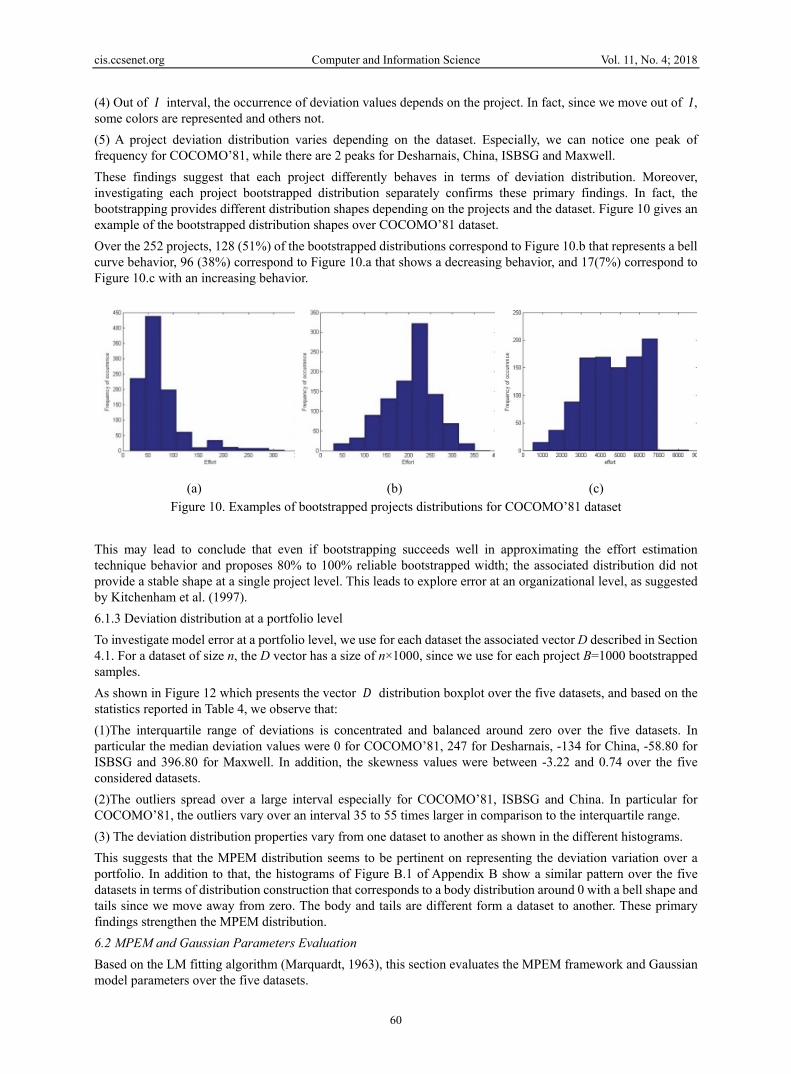
(4) Out of 𝐼 interval, the occurrence of deviation values depends on the project. In fact, since we move out of 𝐼, some colors are represented and others not. (5) A project deviation distribution varies depending on the dataset. Especially, we can notice one peak of frequency for COCOMO’81, while there are 2 peaks for Desharnais, China, ISBSG and Maxwell. These findings suggest that each project differently behaves in terms of deviation distribution. Moreover, investigating each project bootstrapped distribution separately confirms these primary findings. In fact, the bootstrapping provides different distribution shapes depending on the projects and the dataset. Figure 10 gives an example of the bootstrapped distribution shapes over COCOMO’81 dataset. Over the 252 projects, 128 (51%) of the bootstrapped distributions correspond to Figure 10.b that represents a bell curve behavior, 96 (38%) correspond to Figure 10.a that shows a decreasing behavior, and 17(7%) correspond to Figure 10.c with an increasing behavior.
(a) (b) (c) Figure 10. Examples of bootstrapped projects distributions for COCOMO’81 dataset
This may lead to conclude that even if bootstrapping succeeds well in approximating the effort estimation technique behavior and proposes 80% to 100% reliable bootstrapped width; the associated distribution did not provide a stable shape at a single project level. This leads to explore error at an organizational level, as suggested by Kitchenham et al. (1997). 6.1.3 Deviation distribution at a portfolio level To investigate model error at a portfolio level, we use for each dataset the associated vector D described in Section 4.1. For a dataset of size n, the D vector has a size of n×1000, since we use for each project B=1000 bootstrapped samples. As shown in Figure 12 which presents the vector 𝐷 distribution boxplot over the five datasets, and based on the statistics reported in Table 4, we observe that: (1)The interquartile range of deviations is concentrated and balanced around zero over the five datasets. In particular the median deviation values were 0 for COCOMO’81, 247 for Desharnais, -134 for China, -58.80 for ISBSG and 396.80 for Maxwell. In addition, the skewness values were between -3.22 and 0.74 over the five considered datasets. (2)The outliers spread over a large interval especially for COCOMO’81, ISBSG and China. In particular for COCOMO’81, the outliers vary over an interval 35 to 55 times larger in comparison to the interquartile range. (3) The deviation distribution properties vary from one dataset to another as shown in the different histograms. This suggests that the MPEM distribution seems to be pertinent on representing the deviation variation over a portfolio. In addition to that, the histograms of Figure B.1 of Appendix B show a similar pattern over the five datasets in terms of distribution construction that corresponds to a body distribution around 0 with a bell shape and tails since we move away from zero. The body and tails are different form a dataset to another. These primary findings strengthen the MPEM distribution. 6.2 MPEM and Gaussian Parameters Evaluation Based on the LM fitting algorithm (Marquardt, 1963), this section evaluates the MPEM framework and Gaussian model parameters over the five datasets.

cis.ccsenet.org Computer and Information Science Vol. 11, No. 4; 2018
61
Table 4. Deviation statistics over the five datasets
Min Max Mean Median Skewness Kurtosis COCOMO’81 -11302 8945 -91.51 0 -3.22 33.35 Desharnais -20238 11508 -133.38 247.80 0.74 5.47 China -53420 46634 -749.55 -134 -1.39 30.97 ISBSG -55892 29193 -1322.10 -58.80 -1.51 9.42 Maxwell -55630 48642 -1356.40 -396.80 -2.09 13.56
COCOMO’81
Desharnais ISBSG
China
Maxwell
Figure 9. Deviation per project over the five datasets
Table 5. Parameter values of the MPEM over the five datasets Body distribution Left tail Right tail
A1 B1 C1 A2 B2 C2 a1 k1 a2 k2 COCOMO 0.56 -19.41 140.6 0.04842 -75.88 540.3 1.932 -0.9148 19.98 -1.205 ISBSG 0.164 179.2 915.1 0.05831 -373 4473 6348 -1.482 0.9827 -0.6398China 0.3492 -47.6 703.4 0.09164 -444.2 2903 5071 -1.525 2533 -1.526 Desharnais 0.0204 -890.4 1076 0.04901 817.4 2180 1167 -1.419 4.095 -0.7761Maxwel 0.09511 576.3 5731 -0.01519 6285 2760 6064 -1.479 150 -1.138
6.2.1 MPEM Parameters Evaluation Based on Equation (24), to make easier the computational assessment taking into account the negative error values and in order to reduce the number of variables, we suggest the use of the following definitions of the distribution body, denoted 𝐵, the left tail 𝑇 and the right tail 𝑇 given by Equations 33-35 respectively:
𝐵(𝑥) = 𝐴 𝑒 ( ) + 𝐴 𝑒 ( ) (33)

cis.ccsenet.org Computer and Information Science Vol. 11, No. 4; 2018
62
𝑇 (𝑥) = 𝑎 |𝑥| (34) 𝑇 (𝑥) = 𝑎 𝑥 (35)
Table 5 summarizes the obtained parameters. In addition, Table B.1 of Appendix B details the 95% confidence intervals associated to each parameter. The overall distribution corresponds to a mixture of two Gaussians for the body and power law distributions for tails as follows: ℎ(𝑥) = 𝐵(𝑥) + 𝑇 (𝑥). 𝟙] , ] + 𝑇 (𝑥). 𝟙[ , [ (36) where 𝛼 and 𝛼 are defined in Equation (24). In practice, Equation (17) did not provide accurate results. In fact, it produces a high discontinuity in the distribution shapes. To overcome this limitation, we vary the shoulders values from min (𝐵 , 𝐵 ) to min (𝐵 , 𝐵 ) − ( , )√ for the left tail and from max(𝐵 , 𝐵 ) to max (𝐵 , 𝐵 ) + ( , )√ for the right tail.
This corresponds to a 3𝜎 interval for classical Gaussians. For each dataset, we choose the first value enabling an almost continuous distribution. Figure 12 gives a visual illustration of the MPEM fitting curves over the five datasets. We can observe that: (1) Over the five datasets, all the frequencies of occurrence are approximated with a value different from 0. (2) The fitting quality varies from a dataset to another. For example, over China and COCOMO’81, the fitting was better than ISBSG, Maxwell or Desharnais. (3) More the deviation presents a regular behavior without oscillations; more the MPEM is efficient. This may lead to conclude that the MPEM framework seems to be representative of deviation distributions over the five datasets. The shoulders used in this study are indicated in Table 6. 6.2.2 Gaussian model parameters evaluation To evaluate the Gaussian model parameters, we used the LM fitting algorithm (Lokan et al., 2001) used for the MPMF fitting. Equation (37) gives the formula used, that corresponds to the probability density of the Gaussian distribution of Equation (1).
ℎ(𝑥) = 𝐴 ∗ 𝑒 ( ) (37)
Table 6. Shoulders values over the five datasets
Shoulders 𝜶𝟏 𝜶𝟐 COCOMO’81 -1080 1080Desharnais -2400 4000ISBSG -6400 6800China -5850 4200Maxwell -6400 6800
Table 7 presents the obtained parameters and the associated 95% confidence intervals. Furthermore, Figure 15 gives a visual representation of the Gaussian fitting over the five considered datasets. Table 7. Parameters values of the Gaussian model over the five dataset A1 B1 C1 COCOMO Adopted value 0.58 -29.37 163.5
95% confidence interval [0.57, 0.59] [-32.86, -25.88] [159.6, 167.3] ISBSG Adopted value 0.18 126.4 1716

cis.ccsenet.org Computer and Information Science Vol. 11, No. 4; 2018
63
95% confidence interval [0.17, 0.20] [24.95, 227.8] [1573, 1860] China Adopted value 0.42 -23.02 945.5
95% confidence interval [0.40, 0.44] [-66.97, 20.93] [895.8, 995.3] Desharnais Adopted value 0.051 231.7 2888
95% confidence interval [0.047, 0.054] [58.62, 404.8] [2643, 3133] Maxwel Adopted value 0.094 155.4 5470
95% confidence interval [0.089, 0.099] [-73, 383.9] [5147, 5793] We can easily notice that: (1) Over the five datasets, the frequencies of occurrence that correspond to the body distribution are approximated, while the tails are not. (2) The fitting quality varies from a dataset to another. In particular, the Gaussian represents better the concentrated distributions such as COCOMO’81. (3) The Gaussian did not present irregular behavior especially tail oscillations such as those of the Maxwell dataset. These observations lead to conclude that the Gaussian distribution captures the deviation body distribution. However, it did not take into account the tails since the Gaussian curve drops exponentially. 6.3 Comparing the MPMF and the Classical Gaussian Model This section compares the MPEM and the Gaussian model performances using the GOF metrics detailed in Section 5.1 over five datasets. 6.3.1 Overall Fit To analyze the overall fit of the MPEM framework, we first perform for both models the Chi-Square 𝜒 goodness of fit test based on the hypothesis H0 and H1 as detailed in Section 5.1. Moreover, we compute the Pearson's statistic 𝑋² defined by Equations (25).
COCOMO’81 Desharnais ISBSG
China
Maxwell
Figure 11. Deviations boxplot over the five datasets

cis.ccsenet.org Computer and Information Science Vol. 11, No. 4; 2018
64
COCOMO’81 Desharnais ISBSG
China
Maxwell
Figure 12. MPEM fitting curve of deviation over the five dataset Since the Gaussian distribution presents null values over the tails, the likelihood ratio 𝐺² cannot be defined. Thus, we only computed the likelihood ratio 𝐺² defined by Equations (26) for the MPEM framework. From Table 8, we can notice that: (1) For both models, 𝑋²values vary form a dataset to another. (2) MPEM has 𝑋² values very small in comparison to those of the Gaussian model: 2.7056e-004 vs. 422 e-004 for COOCMO’81, 8.1798e-004vs. 2177 e-004 for China, 6.1315e-004 vs. 372 e-004 for Desharnais, 48e-004 vs. 1829 e-004 for ISBSG and 50e-004 vs. 335 e-004 for Maxwell. These values show the precision and the quality of the proposed fit. (3) MPEM 𝐺² values vary from -1.38e-02 for ISBSG to 8.40e-03 for China. The negative 𝐺² over ISBSG suggests that the MPEMF overestimates the deviation distribution, which is confirmed by the 𝑋²value. (4) Over the five datasets, the χ test fails to reject the null hypothesis of the MPEM and the Gaussian model at the 0.05 significance level. The associated p values are higher for the MPEM : [0.94,0.99] vs. [0.64,0.85] for the Gaussian model and support the validity of the null hypothesis. Table 8. MPEM and Gausian model goodness of fit metrics and χ test
MPEM Gaussian model
X2 G2 𝝌𝟐test X2 𝝌𝟐test H p-value h p-value
COCOMO’81 2.7056e-004 5.10e-02 0 0.99 422 e-004 0 0.84 China 8.1798e-004 8.40e-03 0 0.98 2177 e-004 0 0.64 Desharnais 6.1315e-004 1.81e-01 0 0.98 372 e-004 0 0.85 ISBSG 48e-004 -1.38e-02 0 0.94 1829 e-004 0 0.67 Maxwell 50e-004 2.03e-01 0 0.94 335 e-004 0 0.85

cis.ccsenet.org Computer and Information Science Vol. 11, No. 4; 2018
65
The obtained results emphasize the pertinence of MPEM since the χ test supports that the MPEM holds the observed frequencies. In addition, the low values of X² and G² underline the high quality of the overall fit. To compare the MPEM and the Gaussian models overall GOF, we compare both models Pearson's statistic X² since the likelihood ratio is not defined for the Gaussian model. Furthermore, we define the following comparison ratio: 𝜌 = ²² (38)
where 𝑋² and 𝑋² are the Gaussian and the MPEM Pearson's statistic as defined by Equation (25) respectively. The comparison ratio 𝜌 measures how much the MPEM outperforms the Gaussian model in terms of overall fit. Table 9. Comparison ratio over the five datasets
Comparison ration ρCOCOMO 155.97 China 266.14 Desharnais 60.67 ISBSG 38.10 Maxwell 6.70
From Figure 17 and Table 9, we can notice that the Gaussian model presents 6 to 267 times higher 𝑋² than the MPEM. This leads to consider that the MPEM outperforms the Gaussian model in terms of overall fit.
Figure 13. MPEM and Gaussian model X² metric histogram over the five datasets
6.3.2 Residuals To analyze the piecewise GOF, we focus on the residuals as defined by Equation (27). They enable emphasizing the misfit between the observed frequencies and the Gaussian model. Figure 14 provides both models residuals boxplots. Moreover, Figure B.3 and B.4 of Appendix B provide both models residuals distributions. From Figure 14 and the statistics of Table 10, we observe that: (1) The MPEM presents negative median values over the five datasets while the Gaussian model has positive ones. (2) Over four datasets (COMOMO’81, Desharnais, Maxwell, and ISBSG) MPEM has an absolute median value 2% to 84% lower than the Gaussian model. Still both models absolute median values were comparable. (3) Over the five datasets, the interquartile range of the Gaussian model was larger than the MPEM one. (4) Over the five datasets, the MPEM residuals median value was almost in the middle of the interquartile range while the Gaussian was more in the lower quartile. (5) Over all datasets except Maxwell, the MPEM presents confined outliers while the Gaussian shows spreading values 17% to 519% wider than the MPEM.

cis.ccsenet.org Computer and Information Science Vol. 11, No. 4; 2018
66
These results lead to conclude that MPEM has a slight tendency to overestimating while the Gaussian model has a tendency to underestimating. Still, in the majority of cases (80% of datasets) MPEM outperforms the Gaussian one in terms of residuals with narrower and better balanced distributions. Table 10. MPEM and Gaussian residuals statistics
MPEM Gaussian model
Min Max Mean Median Kurtosis Skewness Min Max Mean Median Kurtosis Skewness
COCOMO’81
-
0.0062 0.0051
-8.02e-
05
-4.03e-
04 12.9731 0.4916
-
0.0019 0.0284 0.0017
4.56e-
04 29.4329 4.9055
China
-
0.0055 0.007
-2.50e-
04
-3.27e-
04 13.5622 0.7128
-
0.0101 0.0673 0.0029
2.60e-
04 29.6096 4.7976
Desharnais -0.015 0.0229
-1.57e-
04
-9.54e-
04 9.3624 1.116
-
0.0177 0.0267 0.0017
9.74e-
04 11.136 0.6646
ISBSG
-
0.0114 0.0102
-5.46e-
04
-7.36e-
04 10.0984 0.4598
-
0.0392 0.0366 0.0034
1.2e-03
13.7351 -0.1663
Maxwell -0.014 0.0247
-4.22e-
04
-8.55e-
04 12.1038 1.7225
-
0.0109 0.0238 0.0013
8.87e-
05 11.0881 1.9665
COCOMO’81 Desharnais ISBSG
China
Maxwell
Figure 14. Boxplots of residuals over the five dataset
6.3.3 Model quality index The AIC criterion of Equation (29) aims to allow model selection. In fact, the AIC combines the quality of fit to the model parsimony. Table 11 presents the AIC values of MPEM and Gaussian Model. Table 11. MPEM and Gaussian AIC over the five datasets
Dataset AIC MPEM AICGaussian COCOMO 21.19 7.18

cis.ccsenet.org Computer and Information Science Vol. 11, No. 4; 2018
67
China 21.73 7.75 Desharnais 25.88 11.94 ISBSG 23.21 9.42 Maxwell 24.72 10.73
From Table 11, we can notice that: (1) For both MPEM and Gaussian model, the AIC index varies over the five datasets. (2) Over the five datasets, the AIC index of MPEM is higher than that one of Gaussian model. (3) For MPEM, the AIC values were between 21 and 26 while it was between 7 and 12 for the Gaussian model. This may suggest that, MPEM generates an additional “complexity” since it requires a higher number of parameters. In practice, this additional complexity is limited since it corresponds to the classical models (Gaussians and power laws) that do not need important computational resources to set their parameters. The additional number of parameters enables a better fitting quality taking into account tail events. Then, the MPEM remains reasonable in terms of the required number of variables for the obtained results. 7. Threats to Validity This section underlines the main threats of validity of this study. Especially internal, external, content and construct validity are addressed. Internal validity: To overcome the historical dataset selection bias for the effort estimation technique, we used the Jackknife (LOOCV) validation method combined with bootstrapping. This choice was justified by the performances of LOOCV in comparison with cross validation as it generates lower bias and higher variance estimate (Kocaguneli et al., 2013). In addition to that, LOOCV offers the advantage of generating the same results in a particular dataset if the evaluation is replicated, which is not the case for cross validation. Furthermore, the estimation of the best shoulders values for the MPEM can be formally studied since the theoretical Equation (17) did not provide accurate results for our experimentation. External validity: This study uses five datasets which contain 1038 projects. These datasets are from different countries and organizations, sources and features. This makes them appropriate for evaluating the MPEM framework. Content validity: The MPEM investigated model error management over a portfolio of projects. To evaluate the pertinence of our approach, we use the bootstrapping technique over different datasets (Efron, 1979). That enables generating an important number of estimates that are believed to be representative of the effort estimation technique behavior (Moataz et al., 2009). Furthermore, the shoulders values used in this study may need further investigation in order to propose a formal approach based on optimization theory. Construct validity: To evaluate the performances of MPEM, we use different GoF metrics. In particular: the Pearson's statistic and the Likelihood ratio assess the overall goodness of fit (Maydeu-Olivares et al., 2010). The Akaike Information Criterion evaluates the model quality (Akaike, 1973). Finally, the residuals analysis emphasizes the piecewise fit focusing on the source of misfit. 8. Conclusion and future work This paper aimed to deal with model error at an organization level whatever the effort estimation method used. To achieve this objective, a distribution of error over a portfolio of projects was proposed based especially on bootstrapping and tail risk concepts. Since error distribution shows more stability at a portfolio level in comparison to single projects, we model the portfolio error body distribution using a mixture of two Gaussians and the tails using power law. To evaluate the accuracy of MPEM, we used five different datasets with different sizes for a total of 1038 projects, and an Analogy-based effort estimation technique. The Jackknife technique was combined with bootstrapping. In addition, we used goodness of fit metrics in order to measure the overall and the piecewise fit quality. Furthermore, a comparison between the classical Gaussian model and MPEM was conducted based on goodness of fit metrics and the model quality indices. The findings of this study were the following: (RQ1): Is there evidence that model error management is more suitable at a portfolio level than a single project level? In opposition to single project bootstrapped distributions, the portfolio distributions showed an almost regular

cis.ccsenet.org Computer and Information Science Vol. 11, No. 4; 2018
68
pattern over the five datasets with: (1) a concentration of high frequency of occurrence values around zero which corresponds to the body distribution, and (2) out of this interval, we can notice tail values with a decreasing but non null frequencies of occurrence. (RQ2): Does the MPEM distribution suits to the portfolio error over different datasets? The 𝜒 test shows that both the MPEM and the Gaussian models hold statistically describing the observed error distribution. Still, MPEM presents higher p-values. In addition, MPEM outperforms the Gaussian in terms of overall goodness of fit since it presents lower Pearson's statistic. In terms of piecewise fit, MPEM generally outperformed the Gaussian (80% of cases) since its residuals distributions were better balanced with lower median values and presented more confined outliers. (RQ3): Does the MPEM distribution outperform the classical Gaussian approximation? Over the five datasets, in terms of overall goodness of fit, the MPEM provides 6 to 267 times lower Pearson's statistic in comparison with the Gaussian model. In addition, in terms of piecewise goodness of fit, absolute median values of residuals of both models were comparable. Still, in 80% of the datasets (4 datasets), MPEM outperformed the Gaussian model in terms of residuals with narrower and better balanced distributions. Nevertheless, the AIC measure showed that the MPEM generates additional “complexity” since its number of parameters used is higher than the Gaussian one. This additional complexity remains reasonable for the improvement of goodness of fit obtained. Ongoing work investigates the improvement of the proposed MPEM framework by exploring optimization theory in order to deal with shoulders values. In addition to that, further evaluations of the MPEM performances will be carried out over other datasets with other effort estimation techniques to confirm or refute the findings of this study. References Akaike H. (1973). Information theory and an extension of the maximum likelihood principle presented at the 2nd
International Symposium on Information Theory, pages 267-281. Amazal, F. A., Idri, A., & Abran, A. (2014). An Analogy-Based Approach to Estimation of Software Development
Effort Using Categorical Data. IWSM Mesura, 31, 252-262. https://doi.org/10.1109/IWSM.Mensura.2014.31 Angelis, L., & Stamelos, J. (2000). A simulation tool for efficient analogy-Based cost estimation. Empirical
Software Engngineering, 5, 35-68. https://doi.org/10.1023/A:1009897800559 Azzeh, M., Neagu D., & Cowling, P. (2008). Improving Analogy Software Effort Estimation using Fuzzy Feature
Subset Selection Algorithm. Presented at the 4th International Workshop on Predictive Models in Software Engineering, 71-78. https://doi.org/10.1145/1370788.1370805
Azzeh, M., Neagu, D., & Cowling, P. I. (2011). Analogy-based software effort estimation using Fuzzy numbers. Journal of Systems and Software, 84, 270-284, 2011. https://doi.org/10.1016/j.jss.2010.09.028
Bagdonavicius, V., & Nikulin, M. S. (2011). Chi-squared goodness-of-fit test for right censored data. The International Journal of Applied Mathematics and Statistics, 24, 30-50.
Behboodian, J. (1970). On the modes of a mixture of two normal distributions, Technometrics. https://doi.org/10.1080/00401706.1970.10488640
Bhansali, V. (2008). Tail Risk Management: Why Investors Should Be Chasing Their Tails, Edition. PIMCO. Bruce, L. G. (1995). Mixture models: theory, geometry and applications presented at NSF-CBMS Regional
Conference Series in Probability and Statistics, Hayward, CA. ISBN: 0-94-0600-32-3 Coles, S. (2001). An introduction to statistical modeling of extreme values, Edition London: Springer-Verlag.
ISBN 978-1-4471-3675-0 Deharnais, J. (1989). Analyse statistique de la productivitie des projects de development en informatique à partir
de la technique des points des fontion, Quebec university. Efron, B. (1979). Bootstrap methods: Another look at the jackknife, The Annals of Statistics.
https://doi.org/10.1214/aos/1176344552 Efron, B., & Tibshirani, R. (1993). An Introduction to the Bootstrap, Edition Boca Raton: Chapman & Hall/CRC. Feller W. (1971). An Introduction to Probability Theory and Its Applications, Edition New York: Wiley.
ISBN: 9780471257080 Frühwirth-Schnatter S. (2006). Finite Mixture and Markov Switching Models, Edition Springer. ISBN:

cis.ccsenet.org Computer and Information Science Vol. 11, No. 4; 2018
69
9780387357683. Guerriero V. (2012). Power Law Distribution: Method of Multi-scale Inferential Statistics. Journal of Modern
Mathematics Frontier, 1, 21-28. Idri, A., Abran, A., Khoshgoftaar, T., & Robert, S. (2002 September), Investigating Soft Computing in Case-Based
Reasoning for Software Cost Estimation. International Journal of Engineering Intelligent Systems, 10, 147-157.
Idri, A., Amazal, F. A., & Abran, A. (2015). Accuracy Comparison of Analogy-Based Software Development Effort Estimation Techniques. International Journal of Intelligent Systems, 10, 1-25. https://doi.org/10.1002/int.21748
Kenney, J. F., & Keeping, E. S. (1951). Mathematics of Statistics, Edition Princeton: Van Nostrand. Kraitchik, M. (1942). The Error Curve, Edition New York: W. W. Norton. Levenberg, K. (1944). A Method for the Solution of Certain Non-Linear Problems in Least Squares. Quarterly of
Applied Mathematics, 2, 164-168. https://doi.org/10.1090/qam/10666 Li, Y. F., Xie, M., & Goh, T. N. (2009). A study of project selection and feature weighting for analogy based
software cost estimation. Journal of Systems and Software, 82, 241-252. https://doi.org/10.1016/j.jss.2008.06.001
MacCallum, R. C., Roznowski, M., & Necowitz, L. B. (1992). Model modification in covariance structure analysis: The problem of capitalization on chance. Psychological Bulletin, 111, 490-504.
MacCallum, R. C., Wegener, D. T., Uchino, B. N., & Fabrigar, L. R. (1993). The problem of equivalent models in applications of covariance structure analysis. Psychological Bulletin, 114, 185-199.
Marquardt, D. (1963). An Algorithm for Least-Squares Estimation of Nonlinear Parameters. SIAM Journal on Applied Mathematics, 11, 431-441. http://dx.doi.org/10.1137/0111030
Maxwell, K. D. (2002). Applied Statistics for Software Managers, Edition Englewood Cliffs: NJ. Prentice-Hall. Maydeu-Olivares A. and Garcıa-Forero C. (2010). Goodness-of-Fit Testing. International Encyclopedia of
Education, 7, 190-196. Menzies, T., Caglayan, B., Kocaguneli, E., Krall, J., Peters, F., & Turhan, B. (2012). The promise repository of
empirical software engineering data. Retrieved from http://terapromise.csc.ncsu.edu Michelle, G. K., Cartwright, M., Chen, L., & Shepperd, M. J. (2000 January). Experiences Using Case-Based
Reasoning to Predict Software Project Effort, In Proceeding of the 4th International Conference on Empirical Assessment in Software Engineering, pages 1-22. https://doi.org/10.1.1.34.6648
Milios, D., Stamelos, I., & Chatzibagias, C. (2011). Global Optimization of Analogy-Based Software, In Proceeding of EANN/AIAI, 350-359. https://doi.org/10.1007/978-3-642-23960-1_42
Morrison, D. G., & Schmittlein, D. C. (1980). Jobs, strikes, and wars: Probability models for duration. Organizational Behavior and Human Performances, 25. https://doi.org/10.1016/0030-5073(80)90065-3
Papoulis, A. (1984). Probability, Random Variables, and Stochastic Processes, Edition New York: McGraw-Hill. Quenouille, A. M. H. (1956 Febuary). Notes on Bias in Estimation. Biometrika, 43, 353-360. Robertson, C. A., & Fryer, J. G. (1969). Some descriptive properties of normal mixtures, Scandinavian Actuarial
Journal. https://doi.org/10.1080/03461238.1969.10404590 Spiegel, M. R. (1992). Theory and Problems of Probability and Statistics, Edition New York: McGraw-Hill. Taleb, N. N. (2015). Doing Statistics Under Fat Tails: The Program. Taleb, N. N. (2010). The Black Swan: the impact of the highly improbable, Edition London: Penguin. Tukey, J. (1958). Bias and confidence in not-quite large samples, Ann Math Statist. Wu, D., Li, J., & Liang, Y. (2013). Linear combination of multiple case-based reasoning with optimized weight
for software effort estimation. Journal of Supercomputing, 64, 898-918. https://doi.org/10.1007/s11227-010-0525-9
Boehm, B. (1984 January). Software Engineering Economics. IEEE Transactions on Software Engineering, 4, 4-21. https://doi.org/10.1109/TSE.1984.5010193
Kitchenham, B., & Linkman, S. (1997 May). Estimates, Uncertainty and Risk. Journal IEEE Software, pages 69-

cis.ccsenet.org Computer and Information Science Vol. 11, No. 4; 2018
70
74. https://doi.org/10.1109/52.589239 Shepperd, M., & Schofield, C. (1997 November). Estimating Software Project Effort Using Analogies. IEEE
Transactions on Software Engineering, 2, 736-743. https://doi.org/10.1109/32.637387 Idri, A., Abran, A., & Kjiri, L. (March 2000). COCOMO Cost Model Using Fuzzy Logic, In Proceeding of the 7th
International Conference of Fuzzy Theory and Techniques, 219-223. Lokan, C., Wright, T., Hill, P., & Stringer, M. (2001 September). Organizational benchmarking using the ISBSG
Data Repository. IEEE Software, 18, 26-32. https://doi.org/10.1109/52.951491 Stamelos, I., & Angelis, L. (2001 November). Managing uncertainty in project portfolio cost estimation.
Information and Software Technology, 43, 759-768. https://doi.org/10.1016/S0950-5849(01)00183-5 Idri, A., Zahi, A., & Abran, A. (2006, November). Software Cost Estimation by Fuzzy Analogy for Web
Hypermedia Applications, In Proceeding of the International Conference on Software Process and Product Measurements, 53-62.
Jørgensen, C., & Shepperd, M. (2007 January). A systematic review of software development cost estimation studies. IEEE Transactions on Software Engineering, 33, 33-53. http://doi.ieeecomputersociety.org/10.1109/TSE.2007.3
Patil, M. V. (2007 May). Software effort estimation and risk analysis - A case study. In the International Conference on Information and Communication Technology in Electrical Sciences, IET-UK, 1002-1007.
Vineer, B. (2008 December). Tail Risk Management: Why Investors Should Be Chasing Their Tails, PIMCO, pages 68-76.
Moataz, A., & Muzaffar, Z. (2009 March), Handling imprecision and uncertainty in software development effort prediction: A type-2 fuzzy logic based framework. Information and Software Technology, 51, 640-654. https://doi.org/10.1016/j.infsof.2008.09.004
Seo, Y. S., Yoon, K. A., & Bae, D. H. (2009 December). Improving the Accuracy of Software Effort Estimation Based on Multiple Least Square Regression Models by Estimation Error-Based Data Partitioning. Asia-Pacific Software Engineering Conference, 3-10. https://doi.org/10.1109/APSEC.2009.57
Wen, J., Li, S., & Tang L. (2009 December). Improve analogy-based software effort estimation using principal components analysis and correlation weighting, In Proceeding of Asia-Pacific Software Engineering Conference, 179-186. https://doi.org/10.1109/APSEC.2009.40
Wen, J., Li, S., Lin, Z., Huc, Y., & Huang, C. (2012 January). Systematic literature review of machine learning based software development effort estimation models. Information and Software Technology, 54, 41-59. https://doi.org/10.1016/j.infsof.2011.09.002
Idri, A., & Amazal, F. A. (2012 August). Software cost estimation by fuzzy analogy for ISBSG repository presented at the 10th International FLINS conference on Uncertainty Modeling in Knowledge Engineering and Decision Making, 863-868. https://doi.org/10.1142/9789814417747_0138
Kashyap, D., & Misra, A. K. (2013 March). An Approach for Software Effort Estimation Using Fuzzy Numbers and Genetic Algorithm to Deal with Uncertainty. Computer Science and Information Technology, 3, 57-66. https://doi.org/10.5121/csit.2013.3407
Kocaguneli, E., & Menzies, T. (2013 July). Software effort models should be assessed via leave-one-out validation. Journal of Systems and Software, 86, 1879-1890. https://doi.org/10.1016/j.jss.2013.02.053
Idri, A., Amazal, F. A., & Abran, A. (2014 August). Analogy-based software development effort estimation: A systematic mapping and review, Information. Software. Technology, 58, 206-230. https://doi.org/10.1016/j.infsof.2014.07.013
Amazal, F. A., Idri, A., & Abran, A. (2014 September). Software Development Effort Estimation Using Classical and Fuzzy Analogy: A Cross-Validation Comparative Study. Intenational Journal Computer Intelligent Applications, 13, 1450013 (19 pages). https://doi.org/10.1142/S1469026814500138
Laqrichia, S., Marmiera, F., Gourca, D., & Nevouxb, J. (2015 May). Integrating uncertainty in software effort estimation using Bootstrap based Neural Networks. In IFAC Symposium on Information Control Problems in Manufacturing, 48, 954-959.
Trevir, N. (2015 November). Fat Tail Risk: What It Means and Why You Should Be Aware Of It, NASDAQ. El Koutbi, S., Idri, A., & Abran, A. (2016 August). A Systematic Mapping Study of Dealing with Error in Software

cis.ccsenet.org Computer and Information Science Vol. 11, No. 4; 2018
71
Development Effort Estimation, In the 42th Euromicro Conference series on Software Engineering and Advanced Applications, pages 140-147. https://doi.org/10.1109/SEAA.2016.39
El Koutbi, S., & Idri, A. (2017 April). Entropy-based Framework Dealing with Error in Software Development Effort Estimation presented at the 12th International Conference on Evaluation of Novel Approaches to Software Engineering, 195-202. https://doi.org/10.5220/0006312901950202
Appendix A Attributes of the five datasets Table A.1 China dataset attributes
Attributes Description AFP adjusted function points Input function points of input Output function points of external output Enquiry function points of external enquiry File function points of internal logical files or entity references Interface points of external interface added Added function points of new or added functions Changed function points of changed functions Deleted function points of deleted functions PDR_UFP normalized level 1 productivity delivery rate norm NPDR_AFP normalized productivity delivery rate NPDU_UFP productivity delivery rate (adjusted function points) Resource Team type Dev.Type development type Duration total elapsed time for the project
Table A.2 COCOMO81 dataset attributes Attributes Description SIZE Software Size DATA Database Size TIME Execution Time Constraint STOR Main Storage Constraint VIRTMIN, VIRT MAJ
Virtual Machine Volatility
TURN Computer Turnaround ACAP Analyst Capability AEXP Applications Experience PCAP Programmer Capability VEXP Virtual Machine Experience LEXP Programming Language Experience SCED Required Development
Table A.3 Desharnais dataset attributes
Attributes Description ExpEquip Team experience measured in years ExpProjMan Team manager experience measured in years Transactions Transactions is a count of basic logical transactions in the system
(function points) Entities Entities is the number of entities in the systems data model (function
points) Adj_Factor Function point complexity adjustment factor (Total Processing
Complexity) RawFPs Unadjusted function points

cis.ccsenet.org Computer and Information Science Vol. 11, No. 4; 2018
72
Table A.4 Maxwell dataset attributes
Attributes Description Time Execution Time Constraint App Application type Har Hardware platform used Dba Database type used Ifc User interface Source Project source Telonuse Telon use Nlan Number of development languages usedT01 Customer participation T02 Development environment adequacy T03 Staff availability T04 Standards use T05 Methods use T06 Tools use T07 Software’s logical complexity T08 Requirements volatility T09 Quality requirements T10 Efficiency requirements T11 Installation requirements T12 Staff analysis skills T13 Staff application knowledge T14 Staff tool skills T15 Staff team skills Duration Total elapsed time for the project Size Application size
Table A.5 ISBSG dataset attributes Attributes Description UBBU User Base - Business Units (Number of business units that the
system services) UBL
User Base - Locations (Number of physical locations being serviced/supported by the installed system).
UBCU User Base - Concurrent Users (Number of users using the system concurrently).
VAF Value Adjustment Factor; MTS Max Team Size IC Input Count OC Output Count EC Enquiry Count FC File Count IFC Interface Count
Appendix B Empirical results Table B.1 MPEM parameters confidence interval
Body distribution Left tail Right tail A1 B1 C1 A2 B2 C2 a1 k1 a2 k2
COCOMO’81
[0.5516, 0.5684]
[-22.67,-16.15]
[135.6, 145.6]
[0.04, 0.05][-99.91, -51.85]
[487.1, 593.5]
[-414.7, 418.6]
[-28.24, 26.41]
[-4200, 4240][-29.09, 26.68]
ISBSG [0.1546, 0.1733]
[143.6, 214.8]
[836.3, 993.9]
[0.05128, 0.06534]
[-606.7, -139.3]
[4068, 4877]
[-2.982e+5, 3.109e+5]
[-6.654, 3.69]
[-133.7, 135.7]
[-15.02, 13.74]

cis.ccsenet.org Computer and Information Science Vol. 11, No. 4; 2018
73
China [0.3405, 0.3579]
[-70.44, -24.76]
[673.3, 733.5]
[0.08389, 0.0994]
[-540.2, -348.2]
[2747, 3058]
[-6.041e+5, 6.142e+5]
[-14.76, 11.71]
[-5.142e+5, 5.193e+005]
[-24.39, 21.34]
Desharnais [-0.01687, 0.05767]
[-1321, -459.6]
[-128.5, 2280]
[0.03255, 0.06547]
[-260.2, 1895]
[1421, 2939]
[-1.991e+4, 2.225e+4]
[-3.588, 0.7511]
[-192.1, 200.3]
[-6.246, 4.694]
Maxwell [0.08756, 0.1027]
[-478.8, 1631)]
[4713, 6750]
[-0.04089, 0.01051]
[4691, 7880]
[-459.2, 5979]
[-2.592e+5, 2.713e+5]
[-6.188, 3.23]
[-1.009e+4, 1.039e+4]
[-8.349, 6.074]
COCOMO’81 Desharnais
ISBSG China
Maxwell
Figure B.1. Portfolio deviation over the five considered datasets
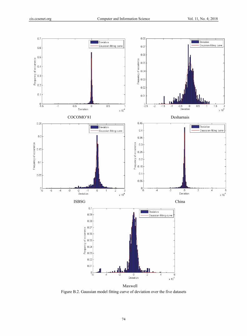
cis.ccsenet.org Computer and Information Science Vol. 11, No. 4; 2018
74
COCOMO’81 Desharnais
ISBSG China
Maxwell
Figure B.2. Gaussian model fitting curve of deviation over the five datasets

cis.ccsenet.org Computer and Information Science Vol. 11, No. 4; 2018
75
COCOMO’81 Desharnais ISBSG
China
Maxwell
Figure B.3. MPEM fitting residuals
COCOMO’81 Desharnais ISBSG
China
Maxwell
Figure B.4. Gaussian model fitting residuals Copyrights Copyright for this article is retained by the author(s), with first publication rights granted to the journal. This is an open-access article distributed under the terms and conditions of the Creative Commons Attribution

cis.ccsenet.org Computer and Information Science Vol. 11, No. 4; 2018
76
license (http://creativecommons.org/licenses/by/4.0/).