software defect prediction using machine learning on test
TRANSCRIPT

Thesis no: MECS-2014-06
Software defect prediction using machinelearning on test and source code metrics
Mattias Liljeson Alexander Mohlin
Faculty of ComputingBlekinge Institute of TechnologySE–371 79 Karlskrona, Sweden

This thesis is submitted to the Faculty of Computing at Blekinge Institute of Technology in partialfulfilment of the requirements for the degree of Master of Science in Engineering: Game and SoftwareEngineering and Master of Science in Engineering: Computer Security. The thesis is equivalent to20 weeks of full-time studies.
Contact Information:Author(s):Mattias Liljeson Alexander MohlinE-mail:[email protected], [email protected]
External advisor:Johan PiculellEricsson AB
University advisor:Michael UnterkalmsteinerDepartment of Software Engineering
Faculty of Computing Internet : www.bth.seBlekinge Institute of Technology Phone : +46 455 38 50 00SE–371 79 Karlskrona, Sweden Fax : +46 455 38 50 57

Abstract
Context. Software testing is the process of finding faults in software whileexecuting it. The results of the testing are used to find and correct faults.Software defect prediction estimates where faults are likely to occur insource code. The results from the defect prediction can be used to opti-mize testing and ultimately improve software quality. Machine learning,that concerns computer programs learning from data, is used to build pre-diction models which then can be used to classify data.Objectives. In this study we, in collaboration with Ericsson, investigatedwhether software metrics from source code files combined with metricsfrom their respective tests predicts faults with better prediction perfor-mance compared to using only metrics from the source code files.Methods. A literature review was conducted to identify inputs for an ex-periment. The experiment was applied on one repository from Ericsson toidentify the best performing set of metrics.Results. The prediction performance results of three metric sets are pre-sented and compared with each other. Wilcoxon’s signed rank tests areperformed on four different performance measures for each metric set andeach machine learning algorithm to demonstrate significant differences ofthe results.Conclusions. We conclude that metrics from tests can be used to predictfaults. However, the combination of source code metrics and test metricsdo not outperform using only source code metrics. Moreover, we concludethat models built with metrics from the test metric set with minimal infor-mation of the source code can in fact predict faults in the source code.
Keywords: Software defect prediction, Software testing, Machine learn-ing
i

Acknowledgements
We would like to thank our university supervisor, Michael Unterkalmsteiner, for greatguidance regarding the conduction of a degree project and scientific methods. Wewould also like to him for giving feedback on the project and the thesis during itsdevelopment. We would like to thank our industry supervisors Johan Piculell andJoachim Nilsson for continuous feedback during the experiment implementation, themetric collection process and the results analysis. Lastly, we would like to thank JonasZetterquist and Ericsson for making this degree project and ultimately the thesis pos-sible by allowing us to work closely with the software development teams and givingus access to Ericsson’s source code repositories.
ii

Contents
Abstract i
1 Introduction 11.1 Motivation . . . . . . . . . . . . . . . . . . . . . . . . . . . . . . . . 11.2 Scope and limitations . . . . . . . . . . . . . . . . . . . . . . . . . . 21.3 Research questions . . . . . . . . . . . . . . . . . . . . . . . . . . . 31.4 Thesis outline . . . . . . . . . . . . . . . . . . . . . . . . . . . . . . 4
2 Background and related work 52.1 ML . . . . . . . . . . . . . . . . . . . . . . . . . . . . . . . . . . . 52.2 Software metrics . . . . . . . . . . . . . . . . . . . . . . . . . . . . 7
2.2.1 Static code metrics . . . . . . . . . . . . . . . . . . . . . . . 72.2.2 Dependency metrics . . . . . . . . . . . . . . . . . . . . . . 82.2.3 Process metrics . . . . . . . . . . . . . . . . . . . . . . . . . 92.2.4 Test metrics . . . . . . . . . . . . . . . . . . . . . . . . . . . 92.2.5 Combinations of metrics . . . . . . . . . . . . . . . . . . . . 102.2.6 Feature selection . . . . . . . . . . . . . . . . . . . . . . . . 10
3 Method 123.1 Literature review . . . . . . . . . . . . . . . . . . . . . . . . . . . . 12
3.1.1 Study selection . . . . . . . . . . . . . . . . . . . . . . . . . 133.1.2 Study quality assessment . . . . . . . . . . . . . . . . . . . . 133.1.3 Synthesis of extracted data . . . . . . . . . . . . . . . . . . . 143.1.4 Threats to validity . . . . . . . . . . . . . . . . . . . . . . . 143.1.5 Answers to research questions 1 – 3 . . . . . . . . . . . . . . 14
3.2 Experiment . . . . . . . . . . . . . . . . . . . . . . . . . . . . . . . 153.2.1 Threats to validity . . . . . . . . . . . . . . . . . . . . . . . 163.2.2 Experiment outline . . . . . . . . . . . . . . . . . . . . . . . 17
4 Experiment implementation 194.1 Data collection . . . . . . . . . . . . . . . . . . . . . . . . . . . . . 19
4.1.1 Identify faulty files . . . . . . . . . . . . . . . . . . . . . . . 204.1.2 Collection of process metrics . . . . . . . . . . . . . . . . . . 204.1.3 Collection of static code metrics . . . . . . . . . . . . . . . . 21
iii

4.1.4 Collection of test and dependency metrics . . . . . . . . . . . 214.2 Metric sets . . . . . . . . . . . . . . . . . . . . . . . . . . . . . . . . 214.3 Model building . . . . . . . . . . . . . . . . . . . . . . . . . . . . . 23
4.3.1 ML algorithms . . . . . . . . . . . . . . . . . . . . . . . . . 234.3.2 Feature selection . . . . . . . . . . . . . . . . . . . . . . . . 244.3.3 Model evaluation . . . . . . . . . . . . . . . . . . . . . . . . 24
5 Results 275.1 Accuracy . . . . . . . . . . . . . . . . . . . . . . . . . . . . . . . . 285.2 Precision . . . . . . . . . . . . . . . . . . . . . . . . . . . . . . . . 305.3 Recall . . . . . . . . . . . . . . . . . . . . . . . . . . . . . . . . . . 315.4 F-measure . . . . . . . . . . . . . . . . . . . . . . . . . . . . . . . . 325.5 Comparison to other studies . . . . . . . . . . . . . . . . . . . . . . 335.6 Feature selection results . . . . . . . . . . . . . . . . . . . . . . . . . 34
6 Analysis and discussion 406.1 Metric sets results . . . . . . . . . . . . . . . . . . . . . . . . . . . . 406.2 ML algorithm results . . . . . . . . . . . . . . . . . . . . . . . . . . 416.3 Comparison to other studies . . . . . . . . . . . . . . . . . . . . . . 416.4 Hypothesis testing results . . . . . . . . . . . . . . . . . . . . . . . . 416.5 Answers to research questions 2 and 3 . . . . . . . . . . . . . . . . . 426.6 Answers to research questions 4 and 5 . . . . . . . . . . . . . . . . . 426.7 What the results means to Ericsson . . . . . . . . . . . . . . . . . . . 436.8 Lessons learned . . . . . . . . . . . . . . . . . . . . . . . . . . . . . 44
7 Conclusion and Future Work 467.1 Conclusion . . . . . . . . . . . . . . . . . . . . . . . . . . . . . . . 467.2 Future work . . . . . . . . . . . . . . . . . . . . . . . . . . . . . . . 47
References 50
iv
Chapter 1Introduction
In collaboration with Ericsson, we have investigated whether Software Defect Predic-tion (SDP) using test and source code metrics can identify hot-spots, i.e. files in thesource code where defects often occurs. Ericsson has provided realistic industry-gradedata which made our research and development possible and the results applicable toEricsson. A discussion of the background follows as well as the formulation of theproblem statement.
1.1 MotivationThe Ericsson M-commerce division maintains a platform for mobile commerce, writ-ten in the object-oriented programming language Java. Due to the domain, moneytransfers, the requirements for creating qualitative and secure products are highly im-portant. Since the number of defects in products can be an indicator of software quality,Ericsson M-commerce have strict requirements regarding defects in their products.
Before a product can be shipped, it needs to be very well tested. The problem,however, is that it is not feasible to test every path in a program. As an example,Myers et al. [33, p. 10] constructed a toy program with 11 decision points and 15branches. To perform exhaustive path testing on that simple program, it would requiretests for 1014 paths. The number of paths in a realistic program render complete testingimpractical due to the exponential growth of paths. Test management at Ericsson istherefore interested in how they can focus their testing on parts that are likely to bedefective.They have problems identifying the source code files that are likely to failduring testing, though. If the testers were provided with information about files whichmight fail, the testing process could be focused on those files.
The lack of knowledge on what to focus the testing on can also lead to faults slip-ping through to later stages of the development which raises the cost associated withfixing them [4, 50]. Duka and Hribar note that the cost of rework due to faults can belowered by 30-50% by finding faults earlier [16].
This area of study is important because of the cost saving potential it poses toEricsson. If fault prone files are detected and testing is focused on the set of fault pronefiles, the testers can save time by not focusing the testing effort on files that are unlikelyto contain faults and instead use that time to thoroughly test the fault prone files. By
1
Chapter 1. Introduction 2
identifying files likely to fail and focusing unit testing improvements to these areas,the testing process can be made more effective. The external quality1 of the product isalso raised when defects are found and corrected before the product is shipped.
An implementation of a tool that provides testers with information on which filesthat are more likely to fail can lead to some negative effects as well. Developers andtesters may rely too much on the tool and actual faulty files that are not caught by thetool are not considered. This false sense of security can lead to faults slipping to laterstages of the development and, as described before, introduce additional cost whencorrecting these faults.
Several studies that investigate defect prone modules in the source code have beenconducted, even within the domain of telecommunication [1, 2, 25, 54]. This masterthesis differs in its approach, compared to previous studies. The novel approach wepropose is to use metrics from test(s), that are testing the source code file, in a combinedmetric set. To the authors’ knowledge, this approach have not been previously studied.
1.2 Scope and limitationsThis master thesis concerns the investigation and development of a tool for predictingfaulty files which includes the following:
• A tool for extracting metrics from a Source Code Management system (SCM)
• A preprocessing tool for structuring the metrics into a desired format.
• An analysis, together with explanations, of produced results.
• A conclusion of why the results came out as they did.
The thesis do not, however, include;
• The development of a tool for data analysis, as this is done with the existingWeka environment [56].
• The measurement and evaluation of the prediction performance of the tool in aproduction environment.
• The production of a front-end tool for graphical representation of the results.
• The observation of the effect the tool has on real users, e.g. whether the toolleads to a sense of false security by its user, or, on the contrary, to mistrust in thetool.
1The term “Quality” is used in the sense defined by McConnell [29, p. 463]

Chapter 1. Introduction 3
1.3 Research questionsFollowing is the list of research questions this master thesis attempts to answer.
RQ1 - What Machine Learning algorithms have been used for SDP?
Identifying which Machine Learning (ML) algorithms that have been used in previousstudies of SDP is highly important for this master thesis to make sure that it contributesto the research community. [The purpose of this master thesis is to investigate if theprediction performance of metric sets are increased if test metrics are included in theset. By using algorithms used in other studies, [the effects of incorporating test metricscan be directly studied]. The prediction performance of the produced tool can also bemade state of the art as lessons from other studies regarding prediction performancecan be incorporated.
RQ2 - What types of metrics have been used in prior SDP studies?
It is of major importance to recognize what kind of source code metrics that previouslyhave been studied. This makes sure that the results of the study can be compared tothose of other studies, and in turn making sure that the thesis contributes to the researchcommunity.
RQ3 - Are there any existing test metrics or test metric suites?
The answer of this question determines if there are any test metrics available whichcan be incorporated into the tool, or if all test based metrics need to be created forthis master thesis. By using existing metrics, the results of the study can be comparedto those of other studies and the contribution of this master thesis to the scientificcommunity is thus strengthened.
RQ4 - Which ML algorithm(s) provide the best SDP performance?
As this master thesis investigates a novel metric family, test and source code metricscombined, there are no prior studies identifying suitable algorithms. The answer to thisquestion will therefore contribute to the research area.
RQ5 - To what extent do test metrics impact the performance of SDP?
The novelty proposed by this master thesis is to use test metrics together with sourcecode metrics. Therefore it is of importance to demonstrate to which extent the testmetrics really contribute to the SDP performance.

Chapter 1. Introduction 4
1.4 Thesis outlineThis master thesis is structured as follows. Chapter 1 introduces the thesis and its moti-vation. Chapter 2 discusses the thesis background, related work and how our work fit inand contributes to the computer science community. Chapter 3 discusses the scientificmethods chosen for this master thesis. Chapter 4 discusses the experiment implemen-tation, our approach and development methods. Chapter 5 presents the results whileChapter 6 discusses the results and answers the stated research questions. Chapter 7chapter summarizes the thesis, presents conclusions and the final analysis as well asfuture work.
Chapter 2Background and related work
Almost all computer software contain flaws that were introduced during code construc-tion. Over time, some of these defects are discovered, e.g. by quality assurance testing.The later in the development process the defects are discovered and corrected, the morecost is associated with fixing them [4, 50]. It is therefore of major importance to findthe flaws as early as possible.
One way of finding flaws or defects is to perform testing. Myers et al. definessoftware testing as “the process of executing a program with the intent of finding er-rors” [33]. Testing is done at many levels including unit testing, function testing,system testing, regression testing and integration testing. The first level of testing isthe unit test level, where the functionality of a specified section of code is tested. Asstated earlier, it is important to find the defects as early as possible to reduce costs. Byfocusing unit tests on the parts that are most fault prone, defects can be found earlier,and thereby reducing costs.
The process of predicting parts that are fault prone in software is called SDP. Theidea behind SDP is to use measurements extracted from e.g. the source code and thedevelopment process, among others, to find out if these measurements can provideinformation about defects. Studies have shown that testing related activities consumebetween 50% to 80% of the total development time [12]. As this is a substantial part ofthe development process, it is important to focus the testing on the parts where defectsare likely to occur due to its cost saving potential. SDP has been studied since the1970’s where simple equations, with measurements from source code as variables, wasused as prediction techniques [17]. Since then, the focus for prediction techniques hasshifted towards statistical analysis, expert estimations and ML [8]. Of these techniques,ML has proven to be the most successful approach [8, 22].
2.1 MLML is a branch of artificial intelligence concerning computer programs learning fromdata. ML aims at imitating the human learning process with computers, and is basi-cally about observing a phenomenon and generalizing from the observations [24]. MLcan be broadly divided into two categories: supervised and unsupervised learning. Su-pervised learning concerns learning from examples with known outcome for each of
5
Chapter 2. Background and related work 6
the training samples [56, p. 40], while unsupervised learning tries to learn from datawithout known outcome. Supervised learning is sometimes called classification, as itclassifies instances into two or more classes. It is classification that this master thesisfocuses on since information about which files that have already been found faulty,exists in a Trouble Report (TR) database.
There has been a large variety of ML algorithms (also known as classifiers) forsupervised learning from a variety of algorithm families presented in previous SDPstudies. These families includes decision trees, classification rules, neural networksand probabilistic classifiers.
Catal et al. [9] concluded that Naïve Bayes, a probabilistic classifier, performs wellon small 1 data sets. Naïve Bayes assumes that the attributes are independent from eachother. This is rarely the case, but by using feature selection in SDP this assumption doesnot affect the results [53]. Feature selection is described in section 2.2.6
Numerous studies [26, 31, 32, 46, 58] have been using J48, which is a Java im-plementation of the C4.5 decision tree algoritm [43]. These studies shows that thealgorithm does not produce any significantly better or worse results compared to otheralgorithms in the studies, except in [58] where J48 performs among the best algorithms,according to accuracy, precision, recall and f-measure, on publicly available data sets.Arisholm et al. [1] claims that the C4.5 algorithm performs “very well overall”, andsuggests that more complex algorithms are not required.
Random Forest, which classifies by constructing a randomized decision tree in eachiteration of a bagging (bootstrap aggregating) algorithm [56, p. 356], has proven to givehigh accuracy when working with large2 data sets [9]. Bagging is an ensemble learningalgorithm that uses other classifiers to construct decision models [5]. Random Forestcan be seen as a special case of bagging, that uses only decision trees to build predictionmodels [26].
Several studies have tested the ability of neural networks for discriminating be-tween faulty and nonfaulty modules in source code [1, 27, 58]. The results from thesestudies have shown that neural networks perform comparable to other prediction tech-niques. Menzies et al. [31], however, proposed using neural networks for future work,as they thought neural networks were too slow to include in their study.
Another previously used method is JRip, an implementation of RIPPER which is aclassification rule learner [3, 48]. Classification rule learners greatest advantage is thatthey are, in comparison, easier for humans to interpret than corresponding decisiontrees.
Menzies et al. [31] maked use of OneR, a classification rule algorithm, to testthresholds of single attributes. They conclude that OneR is outperformed by the J48decision tree most of the times. Shafi et al. [48] used, in addition to OneR, another clas-sification rule algorithm called ZeroR and was outperformed by OneR. ZeroR predictsthe value of the majority class [56, p. 459]. Arisholm et al. has in two different stud-
1In their case around 20 000 lines of code [9]2In their case up to 460 000 lines of code [9]

Chapter 2. Background and related work 7
ies [1, 2] used the meta-learners Decorate and AdaBoost, together with J48 decisiontree. They claim that Decorate outperforms AdaBoost on small data sets and performscomparably well on large data sets. They do not however disclose their definition of“small” and “large” data sets.
2.2 Software metricsSoftware metrics can be described as a quantitative measurement that assigns numbersor symbols to attributes of the measured entity [18]. An attribute is a feature or propertyof an entity, e.g. length, age and cost. An entity can be the source code of an applicationor a software development process activity. There are several different families ofsoftware metrics. Those that are discussed in this master thesis are presented below.
2.2.1 Static code metricsStatic code metrics are metrics that can be directly extracted from the source code,such as Lines of code (LOC) and cyclomatic complexity.
Source Lines Of Code (SLOC) are a family of metrics centred around the count oflines in source files. The SLOC family contains, among others: Physical LOC (SLOC-P), the total line count, Blank LOC (BLOC), empty lines, Comment LOC (CLOC), lineswith comments, Logical LOC (SLOC-L) and lines with executing statements [41].
The Cyclomatic Complexity Number (CCN), also known as McCabe metric, is ameasure of the complexity of a module’s decision structure, introduced by ThomasMcCabe [28]. CCN is equal to the number of linearly independent paths and is cal-culated as follows: starting from zero, the CCN is incremented by one whenever thecontrol flow of a method splits, i.e. when if, for, while, case, catch, &&, || or ?is encountered in the source code.
Other static code metrics include compiler instruction counts and data declarationcounts.
Object-oriented metrics
A subcategory of static code metrics are object-oriented metrics, since they are alsometrics derived from the source code itself. The Chidamber-Kemerer (CK) Object-Oriented (OO) Metric Suite [10] used in this master thesis consists of eight differentmetrics: six from the original CK metric set and two additional metrics, which followsbelow.
Weighted Methods per Class (WMC) counts the number of methods in a class.
Depth of Inheritance Tree (DIT) counts length of the maximum path from class toroot class.

Chapter 2. Background and related work 8
Number of Children (NOC) counts the number of subclasses for one class.
Coupling Between Objects (CBO) counts the number of other classes to which theclass is coupled, i.e. the usage of methods declared in other classes.
Response For Class (RFC) is the number of methods in the class, added to the num-ber of remote methods called by methods of the class.
Lack of Cohesion in Methods (LCOM) counts the number of methods in a class thatdoes not share usage of some member variables.
The additional OO metrics that are used in the thesis are:
Afferent couplings (Ca) counts how many other classes that use the class (cf. CBO).
Number of Public Methods (NPM) counts how many methods in the class that isdeclared as "public".
Menzies et al. [31] used static code metrics such as SLOC and CCN for defectprediction. They observed that the prediction performance was not affected by thechoice of static code metrics. What does matter is how the chosen metrics are used.Therefore, the choice of learning algorithm is more important than the metrics used forlearning. They measure performance with Probability of Detection (PD) and Proba-bility of False alarms (PF). Using Naïve Bayes with feature selection, they gained aPD of 71% while keeping the PF at 25%. Zhang et al. [59] commented on them usingPD/PF performance measures and proposed the use of prediction and recall instead.
Zhang [58] investigated if there exist a relationship between LOC and defects onpublicly available datasets. He argued that LOC, together with ordinary classificationtechniques (ML algorithms), could be a useful indicator of software quality and that theresults are interesting since LOC is one of the simplest and cheapest software metricto collect.
Nagappan et al. [37] concludes that McCabe’s CCN can be used together withother complexity metrics for defect prediction. They note, however, that no single setof metrics is applicable for all of their projects.
2.2.2 Dependency metricsThe division of the workload of different components3 may be decided in the designphase of software development. This division of tasks can impact the quality of thesoftware. Dependency mapping between source code files could therefore be a possiblepredictor of fault prone components. Schröter et al. [47] proposed a novel approach todetect fault prone source files and packages. They simply collected, for each sourcecode file or package, the import statements and compared these imports to failures in
3Defined in IEEE Standard Glossary [23]

Chapter 2. Background and related work 9
components. In this master thesis we denote this procedure of collecting imports asdependency mapping.
Schröter et al. [47] concluded that the sets of components used in another compo-nent, determines the likelihood of defects. They speculate that this is due to that some“domains are harder to get right than others”. Their results point out that collectingimports on package level yields a better prediction performance than on file level. Stillthe results on file level perform better than random guesses.
2.2.3 Process metricsProcess metrics are metrics that are based on historic changes on source code over time.These metrics can be extracted from the SCM and include, for example, the number ofadditions and deletions from the the code, the number of distinct committers and thenumber of modified lines.
Moser et al. [32] compared the efficiency of using change (process) metrics tostatic code metrics for defect prediction. Their conclusion was that process data con-tains more discriminatory information about defect distribution than the source codeitself, i.e source code metrics. Their explanation to this is that source code metricsare concerned with the human understanding of the code, e.g. many lines of code orcomplexity are not necessarily good indicators of software defects.
Nagappan et al. [34] used metrics concerning code churn, a measure of changes insource code over a specified period of time. They conclude that the use of relative codechurn metrics predict the defect per source file better than other metrics and that codechurn can be used to discriminate between faulty and nonfaulty files.
Ostrand et al. [42] used some process metrics explaining if a file was new and if itwas changed or not. The authors used these metrics in conjunction with other metricsfamilies and found that 20% of the files, identified by the prediction model as mostfault prone, contained on average 83% of the faults.
2.2.4 Test metricsTest code metrics can be made up of the same set of metrics that has been previouslydescribed, but for the source code of the tests. In addition to this, Nagappan [36]introduced a test metric suite called Software Testing and Reliability Early Warningmetric suite (STREW) for finding software defects. STREW is constituted by ninemetrics, in three different families:
Test quantification metrics
SM1 Number of assertions4in testSource LOC
SM2 Number of test casesSource LOC

Chapter 2. Background and related work 10
SM3 Number of assertions in testNumber of test cases
SM4 Test LOC / Source LOCNumber of test cases / Number of source classes
Complexity and OO metrics
SM5 ∑Cyclomatic complexity in test∑Cyclomatic complexity of source
SM6 ∑CBO of test∑CBO of source
SM7 ∑DIT of test∑DIT of source
SM8 ∑WMC of test∑WMC of source
Size adjustment metric
SM9 Source LOCMinimum source LOC
Nagappan et al. conclude that STREW provides an estimate of the software’s quality inan early stage of the development as well as identifying fault prone modules [35]. Fur-ther studies conducted by Nagappan et al. [39] indicates that STREW for Java (STREW-J) metric suite can effectively predict software quality.
2.2.5 Combinations of metricsPrevious studies [6, 32], have combined metrics from several metric families in anattempt to achieve better prediction performance.
Caglayan et al. [6] constructed three different sets of metrics. The first set wasstatic code metrics and the second was repository metrics. The third was the two firsttwo combined. The results from this study showed that while they did not got betterprediction accuracy, they did get a decrease in the false positive rate when using thecombined set.
Moser et al. [32] constructed a static code set, a process metric set and a combinedstatic and process set. They concluded that the combined set performed equally wellas the process set, indicating that it is not worth collecting static code metrics.
2.2.6 Feature selectionFeature (or attribute) selection, is a method for handling large metric sets, to identifywhich metrics contribute to the SDP performance. By using feature selection, redun-dant, and hence non-independent, attributes are removed from the data set [56, p. 93].
4Assertions are code that is used during development that allows a program to check itself duringruntime [29, p. 189]

Chapter 2. Background and related work 11
There are two approaches to feature selection: wrappers and filters. Wrappers usethe ML algorithm itself to select attributes to evaluate the usefulness of different fea-tures. Filters use heuristics based on the characteristics of the data to evaluate thefeatures [20]. The positive effects of using filters over wrappers is that they oper-ate faster [21], and are hence more appropriate for the selection in large feature sets.Another positive effect of using filters is that they can be used together with any ML al-gorithm. However, in most cases they require the classification problem to be discrete,whereas wrappers can be put into use with any classification problem. As wrappersuses the same algorithm for feature selection and classification, the feature selectionprocess must be done for every algorithm used for prediction.
A filter based feature selection approach called Correlation based Feature Selec-tion (CFS), presented by Hall [20], has been used in several studies [1, 2, 9]. Unlikeother filter based feature selection algorithms that evaluate individual features, CFSevaluates subsets of features by taking both the merit of individual features and theirintercorrelations into account [21]. The merit of a feature subset is calculated usingPearson’s correlation, by dividing how predictive a feature group is with the redun-dancy between the features in the subset. If a feature is highly correlated with oneor more of the other features in the feature set, that feature will not be considered tobe included in the reduced feature set. Hall claims that the algorithm is simple, fastto execute and, albeit a filter algorithm, can be extended to support continuous classproblems [21].
Shivaji et al. [49] proposes a feature selection technique for predicting bugs insource code. They show that a small part of the whole feature set led to better classifi-cation results than if using the whole set. After the feature selection process, they gaina prediction accuracy of up to 96% on a publicly available dataset. They do however,train the classifier on the feature selected set, which can imply that the model is over-fitted. Smialowski et al. [51], states that special consideration is required when usingsupervised feature selection. They state that one has to make sure that the data used totest a prediction model is not used in the feature selection process. If all data is usedfor feature selection, the predictive performance of the prediction model will be over-estimated. Arisholm et al. [1, 2] have a negative effect in prediction performance whenusing the reduced data set from feature selection, which can imply that the predictionmodel in [49] is overfitted.

Chapter 3Method
As this master thesis covers a new family of metrics in SDP, namely test metrics,having a broad set of algorithms from multiple categories were deemed important asthe prediction performance of test metrics was unknown. To be able to compare theresults to state of the art research and to gain fair results for the test metrics comparedto the source code only metrics, a broad set of metrics of metrics which have performedwell in prior studies where therefore deemed necessary. With this in mind, a literaturereview was conducted to gain further knowledge of these areas. The results from theliterature review was then used in an experiment. The relationship between these twomethods is visualized in Fig. 3.1. This figure also shows how the answers to researchquestions regarding the literature review acted as input to the experiment.
Literature Review Experiment
RQ 4
RQ 5
RQ 1
RQ 2
RQ 3
Input
Input
Figure 3.1: The relation between methods and research questions
This chapter is divided into two separate parts to mirror the way this master thesisproject was conducted. The first part describes the traditional literature review, whichwas done to gain the required background about software defect prediction, ML, sourcecode metrics and test metrics. The second part documents the experiment that tested thehypothesis: “Source code metrics together with test metrics provide better predictionperformance than SDP using only source code metrics”.
3.1 Literature reviewTo answer the research questions 1 – 3, a literature review was conducted. This wasdone to ensure a thorough understanding of the area of software defect prediction,i.e. which ML algorithms and which set of metrics that have previously been studied.Another reason for doing a literature review was to determine whether the gap in the
12

Chapter 3. Method 13
research, that was identified during the planning stage, really exists. This analysis alsoprovided insight into the state of the art research of the area, where the knowledge ofdomain experts’ contributed to the reliability of this master thesis.
3.1.1 Study selectionThe material for the literature analysis was collected using a bibliographic search en-gine that sources data from article databases, journals and conference proceedings.A search strategy as well as a “Literature Review Protocol”‘(LRP) was developed todistinguish, for the thesis, relevant material.
In the domain of software defect prediction, several systematic literature reviewshave been conducted. The method used in this master thesis was to examine the articlesmentioned from five “Systematic Literature Reviews” (SLR) from 1999 to 2013 [17,8, 7, 22, 44]. These articles were then examined closer in order to determine if theymatched the description outlined in the thesis LRP.
In the LRP it was stipulated that the study selection criteria is based on title andauthor. For the title, only SDP articles, conference proceedings etc. with some sort ofML were selected for further examination, excluding studies using statistical analysisthat were not in the scope of this master thesis. The author or authors of the paperwere also examined. If the author had released two or more papers in the domain, andthe paper was referenced by other papers, the paper was considered as a candidate forfurther examination in the literature review.
The other domain related to this master thesis is test metrics. In order to collectarticles about test metrics, multiple search strings with multiple spelling possibilitieswere created iteratively. The selection of these articles followed the approach describedabove.
3.1.2 Study quality assessmentIn order to assess the articles, several culling steps were conducted. Firstly, the ab-stract of each article was closely examined. If the abstract was related to this masterthesis according to the LRP, the article was rated as approved. If not, the article wasdiscarded. The same procedure was repeated for the conclusion. If the articles passedthe scrutinization of both abstract and conclusion they underwent a detailed study ofthe contents. The overall quality of the article was thereafter rated based on: relevanceto this master thesis, the type of publication and presented prediction performance.
The average score of the allotted rates was then calculated and the articles werecategorized into one out of four categories based on an averaged score. During thescore calculation phase, important passages in the articles were highlighted and taggedto point out why the passage was important.
Chapter 3. Method 14
3.1.3 Synthesis of extracted dataIn order to be able to synthesize the work, a collaboration tool was used. The toolattach a note section to each article which was used to note a summary of the article,what rating the article got and why it was important for this master thesis. The toolalso has the possibility to tag articles, to highlight sections of text and place commentswhere needed. Based on the averaged score in the study quality assessment phase, thearticle was categorized. The tags attached to the articles was used to point out where inthe master thesis the article should be mentioned. The comments and highlights wereused as a basis for the discussions in the thesis.
3.1.4 Threats to validityThe threats to validity in the literature review are mainly concerned with the selectionof studies. The selected studies can have both publication biases and agenda drivenbias. To mitigate the threat of the articles being publication biased, articles from severalSLR’s were chosen. Additionally, several different search strings for finding articlesconcerning the other topic was created iteratively as outlined by Zhang et al. [57]. Byconducting the literature review in this way, chances are better that more aspects of thefield of study are covered. The threat of agenda driven bias, i.e. that the authors of anarticle only produces text that suites their purposes, is also mitigated by following thebefore mentioned procedure.
Another identified threat is that only studies with positive results are published. Itcould happen that studies with similar settings with negative results have been per-formed, but their findings might not get published, or, if published, might not get no-ticed by the research community This threat is difficult to mitigate, but efforts includedusing many SLR’s to broaden the article selection and by using a LRP to minimize theimpact of biased mindsets.
3.1.5 Answers to research questions 1 – 3The results from the literature review was mainly used as input to the ML algorithmselection and metric family selection.
RQ1 - What ML algorithms have been used for SDP?
The main ML algorithms used in prior studies are Bagging, Boosting, Decorate, C4.5,Naive Bayes, Neural networks, Random Forest and RIPPER. These were chosen to beused in the experiment as they have been used in multiple prior studies, are of differentcategories and have shown results indicating that they can be used successfully in SDP.ZeroR and OneR were selected to be used as baseline to test other algorithms’ predic-tion performance. These algorithms are discussed in Section 2.1. The implementationsof these algorithms used in the experiment are presented in Section 4.3.1.

Chapter 3. Method 15
RQ2 - What types of metrics have been used in prior SDP studies?
The main metric families used in prior studies are static code metrics, process metrics,dependency metrics, complexity metrics and object-oriented metrics. These familieswere selected to be used in the experiment as they have been used in multiple priorstudies and have shown results indicating that they can be used successfully in SDP.Object oriented metrics were especially selected as the analysis was done on a objectoriented language and as the STREW-J metrics set depended on the CK metric set. Themetric families are discussed in Section 2.2.
RQ3 - Are there any existing test metrics or test metric suites?
There have been articles published regarding metrics for unit tests and test in general.These articles are a series of articles written by Nachiappan Nagappan on a set ofmetrics called STREW. Applied to Java, these metrics are called STREW-J. These arealso discussed in Section 2.2.4. These were included in the experiment.
3.2 ExperimentTo test the hypothesis “Source code metrics together with test metrics provide betterprediction performance than SDP using only source code metrics”, a factorial experi-ment (using feature selection) was conducted. The two factors in the experiment werethe ML algorithms and the metric sets.
Factor 1Factor 2
Source code met-rics
Test metrics Source code andtest metrics
ML algorithm 1 T_S1 T_U1 T_C1ML algorithm 2 T_S2 T_U2 T_C2. . . . . . . . . . . .ML algorithm n T_Sn T_Un T_Cn
Table 3.1: Visualization of the experiment design. T denotes “Treatment”.
The metric sets comprise metrics from static code analysis, change/process analysisand test metrics among others. These are explained in Section 2.2, while all includedmetrics families are listed in Section 4.1. The different metric sets are defined as fol-lows. The Source code metric set (Srcs) contains only metrics related to the sourcecode itself and their files. The Test source code metric set (Tsts) contains metrics re-lated to the test source code, the respective files and metrics only available to tests,e.g. STREW-J metrics. The Combined metric set (Cmbs) is the combination of both ofthese sets, i.e. the union of them, Cmbs = Srcs ∪ Tsts. These three sets only containsource code metrics from source files that have tests testing them as the datasets would

Chapter 3. Method 16
otherwise differ. Comparisons between the data sets and their results would not bepossible if the data sets would differ.
When constructing the Cmbs and Tsts sets, there is a possibility of contaminationof the data. The risk is that if a source file has been reported as faulty, i.e. a TR has beenissued, a unit test to test the defected file has been created. Thereby, the mere presenceof an unit test can be a clue that a source file is faulty. This problem was mitigated bydividing the collected data set into two separate parts based on a pivot point, a point intime (see Fig. 3.2). Only data older than the pivot point and TRs newer than the pivotpoint were considered. By doing the separation in this way, the unit tests created totest a faulty file was not considered in the prediction, and only unit tests created beforea fault had been reported was included in the metric set.
Time
Commits
Trouble reports
Pivot point
Figure 3.2: Separation of TRs and metric extraction
The prediction model process and evaluation was done three times with a differentset of metrics for each of the n ML algorithms, for a total of n× 3 treatments. In thefirst iteration, only source code metrics were used. In the second iteration, only testmetrics were used and in the third iteration, both source code metrics and test metricswere used. The results from these treatments were then compared to test the hypothesisand to answer research questions RQ4 and RQ5.
3.2.1 Threats to validityThe threats to the validity are mainly the reproducibility and generalizability of theexperiment since the source data is confidential and only comes from one repositoryof one product. This is not only a negative aspect as the data is from a real industryproduct and not a "toy" project. The results should therefore be applicable to similarprojects with similar settings. To mitigate the problem with the lack of reproducibilityand generalizability of the experiment, relevant information about the product is dis-closed. The same experiment can therefore be conducted on similar projects and theresults can be compared.

Chapter 3. Method 17
3.2.2 Experiment outlineThe experiment design consisted of several independent variables and a single depen-dent variable. The independent variables were the ML algorithms and the metrics,identified in the literature review. The treatments were the combinations of these. Thedependent variable was the occurrence of corrections to the file. The experiment, itsvariables, objects and hypotheses are further described below.
Dependent variable
The dependent variable was the occurrence of corrections to a tested file due to TRs.The source code file was asserted as faulty if there had been a correction in that partic-ular file. If no correction had been done to a specific file, it was considered as fault freeand hence not faulty. This approach will however result in that a file that has had a faultin its lifetime, is always considered as faulty. The mitigation to this was to introducea time window and a point in time, a pivot point. The file was only considered faultyif the TR was newer than the pivot point. Metrics from the file were extracted frombefore the time of the pivot point. Furthermore, only files changed in the specified timewindow were used.
Independent variables
The independent variables were the different ML algorithms: AdaBoost (Boosting),Bagging, Decorate, J48 (C4.5), JRip, Multilayer Perceptron1, Naïve Bayes, OneRule,Random Forest and ZeroR. In addition to the ML algorithms, the different metric sets,Srcs, Tsts and Cmbs, were also independent variables.
Treatments
One treatment was the combination of the levels of the two independent variables.In this case the metric set and the ML algorithm. Each treatment in the experiment,in Table 3.1 denoted as "T", produces a separate result. In total, we considered 30treatments in the experiment.
Objects
The objects in the experiment was the files that the metrics was extracted from. Fromthe model built by the treatments, a file was classified as either faulty or not faulty.
Hypothesis
The hypothesis tested in this experiment was: “Source code metrics together with testmetrics provide better prediction performance than SDP using only source code met-
1A neural network implementation

Chapter 3. Method 18
rics”. The corresponding null hypothesis used in the experiment is stated as: “Sourcecode metrics together with test metrics provide equal prediction performance as SDPusing only source code metrics”.
Chapter 4Experiment implementation
As described in the method section, an experiment was performed to test the discrimi-natory power of different metric sets with different ML algorithms. In order to collectthese metrics, a tool for scraping them, together with a tool for building and evaluatingthe prediction models was developed. This chapter describes these tools.
Before collecting metrics and faults, a repository on which to conduct the exper-iment must be selected. The main factors when selecting a repository for this exper-iment was the size in terms of number of files and test coverage1. Larger size waspreferred over smaller in order to make the results more accurate and generalizable.The repository had to have a high test coverage since the central theme in the hypoth-esis was the inclusion of test metrics. Choosing a repository with high test coverageassures that many files are tested and hence minimizes test bias. The selected reposi-tory had about 200 KLOC spread over about 2000 files and a test coverage of around70%.
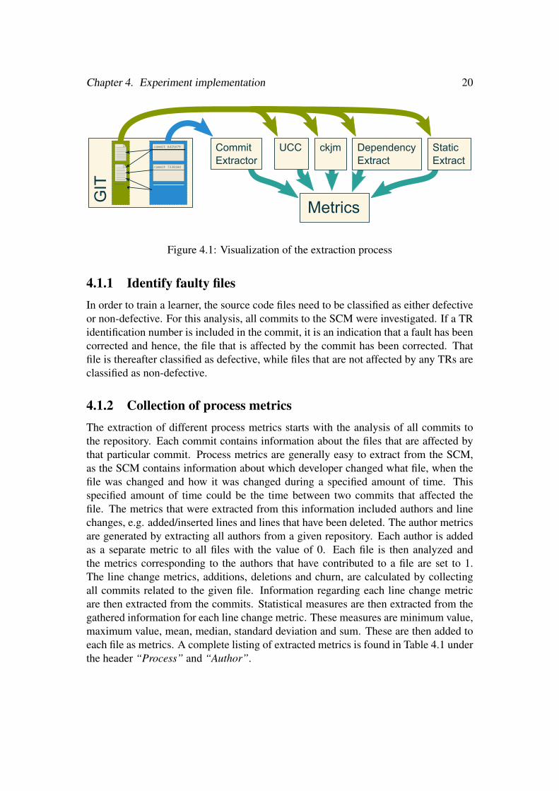
4.1 Data collectionTo be able to collect file level metrics from the SCM Git2, several Groovy3 scripts weredeveloped. These tools were then included in a Gradle4 script as tasks, that allows thescripts to be run sequentially in an automatic manner. The data collection process isoutlined in Fig. 4.1. When possible, external tools used in other studies were used whenextracting metrics as that would give fair results and make the results comparable toother studies. Where there where no tools available or where the available tools werenot applicable due to technical restraints, the metric extraction tools were developedfor the experiment.
1The source code’s degree of testing by tests2http://git-scm.com/3http://groovy.codehaus.org/4http://www.gradle.org/
19
Chapter 4. Experiment implementation 20
commit 6d25679
commit 733818d
commit a22c3e1
Metrics
CommitExtractor
UCC ckjm DependencyExtract
StaticExtract
GIT
Figure 4.1: Visualization of the extraction process
4.1.1 Identify faulty filesIn order to train a learner, the source code files need to be classified as either defectiveor non-defective. For this analysis, all commits to the SCM were investigated. If a TRidentification number is included in the commit, it is an indication that a fault has beencorrected and hence, the file that is affected by the commit has been corrected. Thatfile is thereafter classified as defective, while files that are not affected by any TRs areclassified as non-defective.
4.1.2 Collection of process metricsThe extraction of different process metrics starts with the analysis of all commits tothe repository. Each commit contains information about the files that are affected bythat particular commit. Process metrics are generally easy to extract from the SCM,as the SCM contains information about which developer changed what file, when thefile was changed and how it was changed during a specified amount of time. Thisspecified amount of time could be the time between two commits that affected thefile. The metrics that were extracted from this information included authors and linechanges, e.g. added/inserted lines and lines that have been deleted. The author metricsare generated by extracting all authors from a given repository. Each author is addedas a separate metric to all files with the value of 0. Each file is then analyzed andthe metrics corresponding to the authors that have contributed to a file are set to 1.The line change metrics, additions, deletions and churn, are calculated by collectingall commits related to the given file. Information regarding each line change metricare then extracted from the commits. Statistical measures are then extracted from thegathered information for each line change metric. These measures are minimum value,maximum value, mean, median, standard deviation and sum. These are then added toeach file as metrics. A complete listing of extracted metrics is found in Table 4.1 underthe header “Process” and “Author”.

Chapter 4. Experiment implementation 21
4.1.3 Collection of static code metricsThere are several tools freely available for collecting static code metrics, but they eachhas a rather limited field of application. Therefore, in order to collect several staticcode metrics, several different tools have been used. To collect LOC and other relatedmetrics, Unified Code Count (UCC)5 was used. UCC collect metrics such as SLOC-P,BLOC, CLOC and SLOC-L along with compiler instruction counts and data declara-tion counts. UCC and its features are documented by Nguyen et al. in [41]. The CCNwas extracted using a tool that was developed for this master thesis project.
The CK OO metric suite was calculated using an existing tool called ckjm6 [52].The metrics that are calculated by ckjm constitutes of eight different metrics, six fromthe original CK metric set and two additional metrics, which are listed in section 2.2.1.
4.1.4 Collection of test and dependency metricsThe dependency metrics discussed in Section 2.2.2 were collected through a depen-dency mapping script created for this master thesis.
In this script, all files are opened and all import statements gathered. These im-port statements are then analyzed to see whether the imported files are a part of therepository. If that is the case, they are tested to find out whether they are test related orsource code dependencies. Each file in the repository is then scanned to see whetherthey include a certain dependency. If they do, the dependency is added as a metric witha value of 1. If they do not, the dependency is added as a metric with a value of 0. I.e.each file that has been imported by another file is added as a metric to the file importingit. All of the dependency metrics were collected for both source code and test sourcecode. In the case of this study with a repository of 200K source LOC, the amount ofdependency metrics was around 20 000, in other words the number of unique importstatements.
The eight first metrics from STREW-J listed in subsection 2.2.4 were applied tothe Tsts and Cmbs only as these are test specific metrics. They were collected by syn-thesizing results from the existing metrics from which they are created. The collectionand synthesis of the other test related metrics are elobarated in Section 4.2.
4.2 Metric setsThe extraction of metrics described above results in a single file containing all ex-tracted metrics per file. Another script is then responsible for the creation of threedistinct metric sets, Srcs, Tsts and Cmbs, as described in Section 3.2. This script isalso responsible for calculating the test specific metrics described earlier. All informa-
5http://sunset.usc.edu/research/CODECOUNT/6http://www.spinellis.gr/sw/ckjm/

Chapter 4. Experiment implementation 22
Author Process Dependencies ckjm (OO) Static code Analysis Universal Code Counter (UCC) STREW-J
Author 1 Additions (add) External dep 1 CA BLOC BLOC SM1Author ... Deletions (del) External dep ... CBO BLOC-LOC ratio Compiler directives SM2Author n Commit date External dep n DIT CCN Data declarations SM3
Codechurn (add-del) LCOM CCN-LOC ratio Embedded comments SM4Internal dep 1 NOC CLOC Executable statements SM5
For each of the above: Internal dep ... NPM CLOC-BLOC ratio SLOC-L SM6Min Internal dep n RFC CLOC-LOC ratio SLOC-P SM7Mean WMC LOC LOC SM8Median Test dep 1 Nr of asserts CLOCMax Test dep ... Nr of class defintionsStandard deviation Test dep n Nr of interface definitionsSum Nr of test definitions
Table 4.1: A listing of all the metrics used to build the metric sets
tion needed for calculating these metrics is available in the produced metric file. Thisprocess is visualized in Fig. 4.2.
Metrics
Mapper
Src
TestSrc
Test
Test
TestSrc
Test Test
TestSrc
Test
CombinerSrc
TestSrc
TestSrc
Test
Srcs
SrcSrcSrc
Tsts
Cmbs
Test
Test
Test
Test
TestSrc
Test
SrcTest
SrcTestSrcTestSrcTest
Figure 4.2: Visualization of the mapping and combining process
The mapping between test source code and source code described in Section 3.2is done at this stage. This is done by analyzing the dependency metrics of each file tomap test source code files to source code files. Source code files with no correspondingtest source files are culled so that all three metric sets contain the same files. This isdone so that results from the different sets can be compared as they consist of the samefiles, albeit with different metrics. The mapping is then used when synthesizing testmetrics. All metrics for the mapped tests are gathered per source file and statisticalmeasures are then calculated from the gathered test file metrics. These measures are:minimum value, maximum value, mean, median, standard deviation and sum. Thesemeasures are then added as metrics to the Cmbs and Tsts. For the Cmbs, the metricsfrom the source file are also added. The last step is calculating STREW-J for the Cmbsand Tsts. The dependent metrics from which STREW-J are calculated are fetched andthe calculated STREW-J metrics are added to the sets. As the study only concernsthe identification of faulty source code files, data of faulty test source code files areremoved from the sets. A listing of all the metrics used to build the metric sets ispresented in Table 4.1.

Chapter 4. Experiment implementation 23
4.3 Model buildingTo build the prediction models, file level data from one big repository consisting of200 000 LOC Java source code were used. There exist a large number of smallerrepositories that could have been included in this master thesis project. However, ithas been suggested that, because of that different processes largely depends on theoperating environment, generalizing results between systems and environments mightnot be viable [2, 38].
4.3.1 ML algorithmsAs the experiment was conducted to test the discriminatory power of different metricsets, the ML algorithms included were used with their standard settings in the WEKAenvironment [56]. The algorithms used to build the prediction models in this masterthesis are listed in below:
Naïve Bayes - a simple probabilistic classifier.
J48 - an implementation of the C4.5 decision tree algorithm.
Decorate J48 - Decorate is a meta-learner that builds a diverse ensemble of classifiersusing other learning algorithms [30]. In this case, J48 is used.
Random Forest - that classifies by constructing a randomized decision tree in eachiteration of a bagging (bootstrap aggregating) algorithm [56, p. 356].
OneR - an implementation of 1-rule (1R), which is a simple classification rule algo-rithm.
JRip - an implementation of RIPPER, a classification rule generating algorithm thatoptimizes the rule set. [11].
ZeroR - is a very simple method for generating rules. It simply predicts on the major-ity class of the test data [56, p. 459].
Multilayer perceptron - a neural network that learns trough backpropagation to setthe appropriate weights of the connections [56, p. 235].
AdaBoost - AdaBoost is a meta-learner that, in theory, combines tweaked "weak"learners into a single "strong" learner. In this case, Wekas’ standard setting De-cisionStump, is used.
Bagging - Bagging is also, like Decorate, an ensemble learning algorithm. In thiscase, Wekas’ standard setting REPTree, is used.
Chapter 4. Experiment implementation 24
4.3.2 Feature selectionThe computational complexity of some of the previously mentioned ML algorithmsmakes the model building infeasible to use if all of the features in the dataset is used.As an example, Menzies et al. [31] ruled out neural networks as "they can be veryslow". Therefore, to be able to compare all of the ML algorithms, as the datasets usedin this master thesis project rise up to approximately 20 000 different metrics, featureselection is used to reduce the dataset before building models. As a wrapper uses theML algorithm itself when creating the subset, a new feature selected subset wouldhave to be created for each classifier. Some of the ML algorithms chosen would alsohave to be removed, e.g Multilayer Perceptron, as their execution time would makethem inappropriate for a production setting. This problem became apparent during thedevelopment of the experiment. When choosing a feature selection approach, filteringwas therefore chosen. The tool for feature selection in this master thesis uses CFS,presented by Hall [20]. As the search method for finding the metric subset to evaluatewith CFS, best first search was chosen. This choice was made because of the claim in[20] that it gave slightly better results over other search methods for CFS. The featureselection process was done on the training set in all of the runs of the evaluation processdescribed in Section 4.3.3.
4.3.3 Model evaluationTo evaluate the prediction models produced, 10 times 10-fold cross validation wasperformed. By using 10-fold cross validation, the dataset is separated into 10 somewhatequally large parts. Nine parts out of 10 are used as training data and the featureselection process while the 10th part is used for testing exclusively. This process isrepeated 10 times so that every instances of the data set is used as testing set one time.
In order to guarantee that the distribution of the samples into training and test setwas representative of the distribution of the whole set, stratification was also used in theevaluation process. Stratification means that each fold in the cross validation processgets approximately the same amount of faulty files. If this is not done, a classifierwithin a fold can perhaps be built with no faulty files occurrences, and therefore skewthe result of the whole 10-fold cross validation prediction.
Cross validation can be used in cases where the amount of data is limited, but thereare other advantages compared to other evaluation methods, e.g. the holdout method.When using the holdout method, one part of the data set is used for training and theother for testing, typically two thirds for training and the remaining third for test-ing. This could mean that the samples in the training data is not representative for thewhole data set. One way of mitigating this bias is to use cross validation where all theinstances have been used exactly one time for testing. Witten et al. [56, p.153] statesthat a single 10-fold cross validation might not produce a reliable error estimate. Theystate that the standard way of overcoming this problem is to repeat the 10-fold crossvalidation 10 times and average the results. This means that, instead of conducting 10
Chapter 4. Experiment implementation 25
folds, a total of 100 folds is generated and the error estimate is therefore more reliable.When using feature selection, it is important to remember to take this into account
when performing cross validation. For the prediction not to be skewed, each fold of thecross validation must include a feature selection step, in order to keep test data frombeing present in the training data and hence in the feature selection process. As thefeature selection is conducted in every fold of the 10 times 10-fold cross validation,the process is done 100 times. As both the feature selection process and the learningprocess are computationally intensive, the whole evaluation process consumes a lot oftime. In the case of this study, the complete process took about 4 days to complete adata set with about 20000 features and 1000 instances using a mid-range 2013 laptopwith 8GB RAM and a 1.8Ghz Intel i5 processor.
All results from every fold and every round are recorded in a result file for fur-ther analysis. Hall et al. [22] describes in their systematic literature review differentappropriate performance measures. The result file produced by the evaluation processtherefore contains these measures, i.e. average precision, average recall and averagef-measure. In addition to these performance measures, the average accuracy, the per-centage of the correctly classified instances, of the prediction model is also included.
Precision measures the proportion of the identified files, classified as faulty, that ac-tually are faulty. This is a measure of how good the prediction models are at identifyingactual faulty files. Recall measures the proportion of faulty files which are correctlyidentified as faulty. Recall is a measure of how many faulty files that the predictionmodel is predicted to find. The calculation of accuracy (equation 4.1), precision (equa-tion 4.2) and recall (equation 4.3) makes use of the confusion matrix (fig 4.3) and isdone by;
Accuracy =true positives + true negatives
true positives+ true negatives + false positives + false negatives(4.1)
Precision =true positives
false positives+ true positives(4.2)
Recall =true positives
false negatives+ true positives(4.3)
F-measure (equation 4.4) is a measure that combines both recall and precision andis calculated as
F−measure = 2∗ precision∗ recallprecision+ recall
(4.4)
By collecting these performance measurements, future predictions on unseen filescan be estimated. The whole model building and evaluation process is further describedin the pseudo code in Fig. 4.4.

Chapter 4. Experiment implementation 26
Predicted
ActualPositive Negative
Positive
Negative
True Positive(TP)
False Positive(FP)
True Negative (TN)
False Negative(FN)
Figure 4.3: Confusion matrix
classifierType = {
Naive bayes,
Random Forest,
J48,
...
}
10.times {
randomize instance order
prepare stratified 10-fold cross validation
fold.each{
get training set
get testing set
create feature selection set from training set
record selected features
classifierType.each{
build classifier
test classifier against testing set
record results
}
}
}
Figure 4.4: Pseudo code describing the building and evaluation of the models
For each of the performance measurements, a matched pair Wilcoxon’s signed ranktest was conducted. This was done to demonstrate difference between the ML algo-rithms and the metric sets for each of the performance measurements. As the under-lying data can not be guaranteed to meet the parametric assumptions required by at-test, i.e. it is not guaranteed to be normally distributed, Wilcoxon signed-rank testwas used [24]. Wilcoxon’s signed rank test has been recommended for studies com-paring different algorithms [15]. Due to the large amount of tests being performed,the significance level, α is set to 0.001 This is in line with other studies in the area aswell [1, 2].
If there is a statistical significant difference between one algorithm compared toanother one, using the same metric set, the "better" one wins. The algorithm thathas the most wins for each metric set is considered the best algorithm for that metricset. When the best learning algorithm for each metric set has been determined, theperformance of the different metric sets can be assessed.

Chapter 5Results
This section reports the results from the experiment described in Chapter 3. Runtimeperformance-wise the collection and preprocessing of the metrics were rather quick.It took about 2 hours and about 8 hours respectively. The model building and evalua-tion however took about 4 days using a mid-range 2013 laptop with 8GB RAM and a1.8Ghz Intel i5 processor.
The prediction performance is presented with the four different measures describedin Section 4.3.3. First, the accuracy of the different prediction models on differentfeature selected metric sets is presented and evaluated. Thereafter, the results of f-measure, precision and recall is presented in respective order. This is done to de-termine the best performing ML algorithm to be used for determining the predictionperformance of the different metric sets, that is presented after the ML algorithm eval-uations. Tables and graphs of the performance of prediction models are presented andform the basis of the discussions in the subsections. In the tables and figures, the setsare abbreviated as “src”, “tst” and “cmb” which corresponds to the Srcs, Tsts andCmbs respectively. The original full set of metrics for all source files (abbreviated as“srcRaw”) is also included in the graphs which hints of the repository’s predictionperformance when using ordinary metrics. As the underlying dataset differs from theothers, i.e. it is based on a full set of files and not only those that are tested (describedin Section 3.2), the results of that set can not be directly compared to the other results.It is included in the graphs as a visual cue of the repository’s performance. These setsare explained in detail in Section 3.2.
The tables presented, Tables 5.6 to 5.9, present the outcome from Wilcoxon’ssigned rank tests [55]. Each combination of ML algorithm and metric set is testedagainst all other combinations resulting in 900 Wilcoxon’s signed rank tests. SrcRawis not included in these tables as srcRaw uses a different dataset and can not be com-pared to the other metric sets in this manner. A green cell indicates that the test revealsthat the combination of ML algorithm and metric set perform significantly better thanthe combination tested against. A red cell indicates that the combination performs sig-nificantly worse while a white cell indicates a draw. In addition to the coloured cells,the mean value of the performance measurement studied is presented on each row. Thebest ML algorithm for each of the metric sets is thus the one with the most green cellsin the table. The most predictive metric set is likewise the one with the most green
27

Chapter 5. Results 28
cells in the same table. Total scores for each of the subsets are summarized in thesmall subtable to the right of the main subtable in each table.
The graphs presented in the sections below, Figs. 5.1 to 5.4, gives visual indicationof how the different metric sets perform together with the different ML algorithms.The graphs are box-and-whisker diagrams where the band in the box shows the me-dian, the top and bottom of the box shows third and first quartiles, the whiskers showsminimum and maximum values and circles denote outliers. The box height shows theinterquartile range. The results are grouped together with the other results using thesame algorithm on the X axis. The keys on the X axis labels the different groups withthe algorithm used in that group. The Y axis shows the prediction performance in thegiven measure in form of percentage (
Summaries with the best performing algorithms are also presented in Tables 5.1to 5.4. Their mean values and standard deviations are also shown for each predictionperformance measure. With this table, the performance of the best performing MLalgorithms can quickly be concluded.
A comparison to other studies is also included in Section 5.5 where results fromother studies in the domain are compared to those of this study.
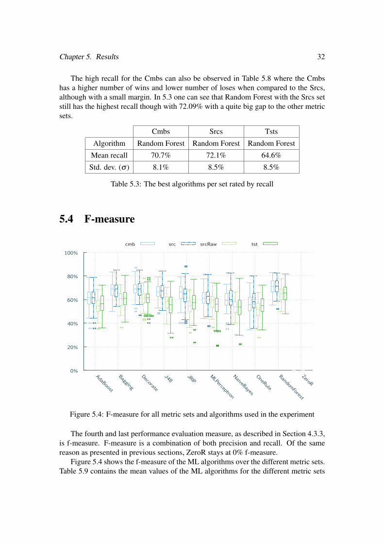
Lastly, in Figs. 5.5 to 5.7, the results of the feature selection process along with thefamilies of the selected features are presented, as these are the features of which themodels are built on.
5.1 AccuracyAccuracy is, as described in Section 4.3.3, the percentage of the correctly classifiedinstances. Figure 5.1 shows the accuracy of the 10 different ML algorithms for the threedifferent metric sets defined in 3.2, i.e Srcs, Tsts and Cmbs. The last ML algorithm inFig. 5.1, ZeroR, is the baseline to test the accuracy of the other algorithms against asdescribed in Section 4.3.1. ZeroR only predicts according to the majority class, on allinstances. It reaches just short of 70% accuracy, which suggests that there are about30% faulty files in the set. This is not at all surprising as the stratification processaims for an evenly distributed dataset. All of the other ML algorithms reach a higheraccuracy on all of the provided metric sets. Most of the results are evenly distributedwith a few exceptions which indicate that the median is a good indicator of the accuracyperformance. There are a few outliers, especially for the Tsts, which indicates a widerspread in the results for that metric set.
Table 5.6 shows which of the ML algorithms that outperform each other for thedifferent metric sets, in terms of accuracy as well as the mean accuracy (described inpercentage) of the modeling techniques for the different metric sets. In Table 5.6, onecan see that the models typically predict, except for ZeroR, 76% to 82% correct. Thebest ML algorithm for the different metric sets, based on accuracy, is determined byperforming a Wilcoxon’s signed rank test as described in Section 4.3.3. As well aswhich ML algorithm that performs the best, the metric set that yields the best accuracy

Chapter 5. Results 29
0%
20%
40%
60%
80%
100%
AdaBoost
Bagging
Decorate
J48JRIP
MLPerceptron
NaiveBayes
OneRule
RandomForest
ZeroR
cmb src srcRaw tst
Figure 5.1: Accuracy for all metric sets and algorithms used in the experiment
can also be seen in the table 5.6.For the accuracy, Random Forest with the Srcs wins and Random Forest with Cmbs
come second with one more tie. There is no statistical significant difference betweenRandom Forest for Srcs and Random Forest Cmbs. Overall, the Tsts performs quitebadly compared to both the Srcs and Cmbs metric sets. It is not however RandomForest that perform best for the Tsts but Bagging which also performs quite well forthe other sets as well. In summary, the Srcs generally scores better than both the Tstsand the Cmbs sets. When comparing the best performing algorithms for each set,shown in Table 5.1, the difference is minimal.
Cmbs Srcs Tsts
Algorithm Random Forest Random Forest Bagging
Mean accuracy 81.7% 81.8% 78.9%
Std. dev. (σ ) 3.5% 3.8% 3.7%
Table 5.1: The best algorithms per set rated by accuracy
Chapter 5. Results 30
0%
20%
40%
60%
80%
100%
AdaBoost
Bagging
Decorate
J48JRIP
MLPerceptron
NaiveBayes
OneRule
RandomForest
ZeroR
cmb src srcRaw tst
Figure 5.2: Precision for all metric sets and algorithms used in the experiment
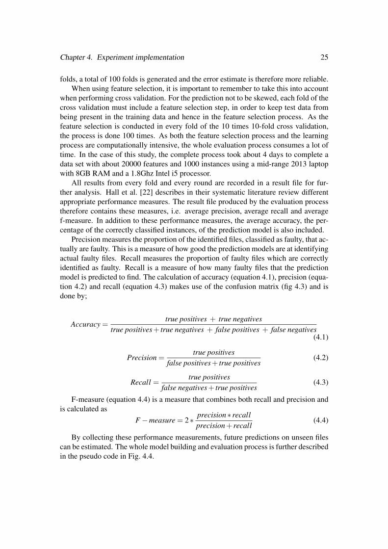
5.2 PrecisionAnother performance evaluation measure, as described in Section 4.3.3 is precision.Precision is the measure of how well the prediction model classifies faulty files thatactually are faulty. A table containing the mean values of the ML algorithms overthe different metric sets together with a figure of how the algorithms perform againsteach other for different metric sets in terms of precision, are presented in Table 5.7and Fig. 5.2. In Fig. 5.2 ZeroR stays at 0% precision as it predict all instances asnot faulty and hence does not find any faulty files. As in accuracy, the Srcs performsbest generally with the Cmbs coming in second and the Tsts last. For two algorithms,Bagging and JRip, the Tsts is the best performing metric set. The results are for themost part not skewed but the spread however is quite large spanning from around 40%to 90% and 50% to 100% in some cases. This can also be seen in Table 5.2 where thestandard deviation is high for all of the three best performing algorithms.
Table 5.7 shows the individual scores for the combination of metric sets and ML al-gorithms. In the case of precision, Bagging performs best in the Cmbs and the Tsts. Inthe Srcs, both Multilayer Perceptron and NaiveBayes scores better, however. Baggingtogether with the Tsts outperforms the other algorithms for the Tsts by margin, though.In summary, the Srcs scores significantly better than both the Tsts and the Cmbs ingeneral. When looking at Table 5.2 the difference between the best performing algo-rithms for the different sets is not that big, though. Surprisingly, the best algorithm forTsts performs better than the best algorithm for Cmbs.

Chapter 5. Results 31
Cmbs Srcs Tsts
Algorithm Bagging Multilayer Perceptron Bagging
Mean precision 73.1% 74.7% 74.1%
Std. dev. (σ ) 8.5% 9.4% 10.1%
Table 5.2: The best algorithms per set rated by precision
5.3 Recall
0%
20%
40%
60%
80%
100%
AdaBoost
Bagging
Decorate
J48JRIP
MLPerceptron
NaiveBayes
OneRule
RandomForest
ZeroR
cmb src srcRaw tst
Figure 5.3: Recall for all metric sets and algorithms used in the experiment
A third performance evaluation measure, as described in Section 4.3.3 is recall.Recall measures how many of the faulty files the prediction model finds. Of the samereason presented in Section 5.2 ZeroR stays at 0% recall. Figure 5.3 shows the preci-sion of the ML algorithms over the different metric sets. Table 5.8 contains the meanvalues of the ML algorithms over the different metric sets together with a figure of howthe algorithms perform against each other for different metric sets in terms of recall.
In Fig. 5.3 one can clearly see that the spread is even larger than it is for the preci-sion, over 70% for Naive Bayes using the Tsts, and that the amount of outliers is largeas well. The spread is however lower for the Cmbs in most cases when compared tothe other sets. As in the other prediction performance measures, the results are not es-pecially skewed. One distinctive feature is that the median is generally higher or aboutthe same for the Cmbs when compared to the Srcs.
Chapter 5. Results 32
The high recall for the Cmbs can also be observed in Table 5.8 where the Cmbshas a higher number of wins and lower number of loses when compared to the Srcs,although with a small margin. In 5.3 one can see that Random Forest with the Srcs setstill has the highest recall though with 72.09% with a quite big gap to the other metricsets.
Cmbs Srcs Tsts
Algorithm Random Forest Random Forest Random Forest
Mean recall 70.7% 72.1% 64.6%
Std. dev. (σ ) 8.1% 8.5% 8.5%
Table 5.3: The best algorithms per set rated by recall
5.4 F-measure
0%
20%
40%
60%
80%
100%
AdaBoost
Bagging
Decorate
J48JRIP
MLPerceptron
NaiveBayes
OneRule
RandomForest
ZeroR
cmb src srcRaw tst
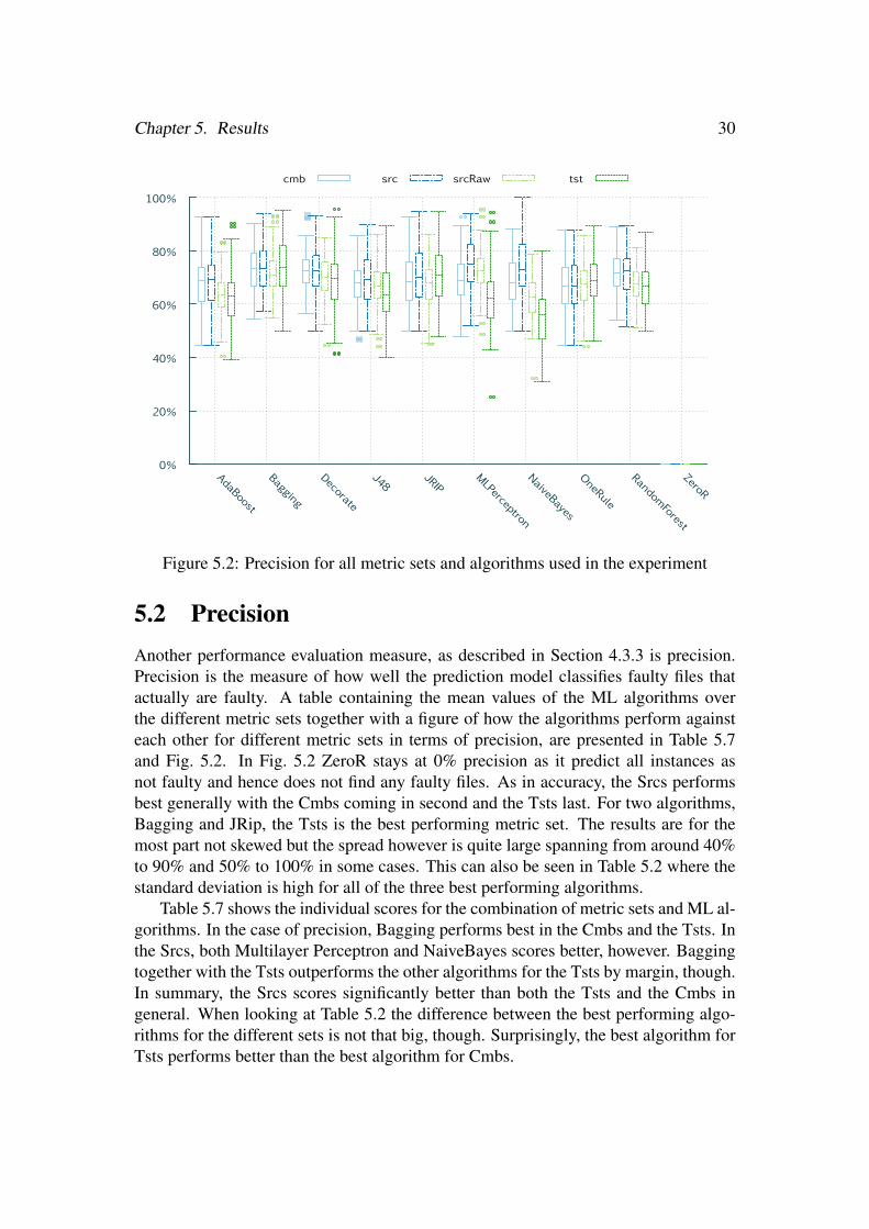
Figure 5.4: F-measure for all metric sets and algorithms used in the experiment
The fourth and last performance evaluation measure, as described in Section 4.3.3,is f-measure. F-measure is a combination of both precision and recall. Of the samereason as presented in previous sections, ZeroR stays at 0% f-measure.
Figure 5.4 shows the f-measure of the ML algorithms over the different metric sets.Table 5.9 contains the mean values of the ML algorithms for the different metric sets

Chapter 5. Results 33
together with a figure of how the algorithms perform against each other for differentmetric sets in terms of f-measure.
Figure 5.4 shows that the Cmbs and Srcs results generally have medians very closeto each other. This can also be seen in 5.9 were the Srcs and Tsts results often resultsin a tie rather than a win or loss. For some algorithms, the Srcs outperform the Cmbs,though, which can be seen in Table 5.9 where the Srcs has more wins and fewer lossescompared to the Cmbs.
Cmbs Srcs Tsts
Algorithm Random Forest Random Forest Random Forest
Mean f-measure 70.9% 71.5% 65.2%
Std. dev. (σ ) 6.3% 6.3% 7.1%
Table 5.4: The best algorithms per set rated by f-measure
5.5 Comparison to other studiesTo ease the comparison to other studies, the mean results for all sets and all perfor-mance measures are compiled in Table 5.5. These values are the ones used in thecomparison in this section.
As accuracy is dependent on the balance of the underlying dataset it is hard tocompare the accuracy results of this study with others. This measure is therefore notwidely discussed in other studies but is a comprehensible measure and is thereforepresented in this study.
Hall et al. has in their systematic literature review gathered results from 208 faultprediction studies [22]. Among those, 48 studies deal with fault prediction on the filelevel. These studies are compared with precision, recall and f-measure. As this study isconducted using the same performance measures as Hall et al. and as they summarizemany studies, the results of this study are compared to the ones compiled by Hall et al.
When the precision is compared to other studies, Srcs and Cmbs performs in gen-eral above the median, while the Tsts performs slightly below the median. For recall,
Cmbs Srcs Tsts
Accuracy 78.9% 79.4% 75.8%
Precision 69.7% 71.4% 66.1%
Recall 60.8% 60.5% 53.0%
F-measure 64.3% 64.7% 57.8%
Table 5.5: Mean prediction performance of the metric sets

Chapter 5. Results 34
the Cmbs and Srcs performs above the median while the Tsts on the other hand per-forms below the median. The results for the f-measure are in general slightly betterthan for other studies where the Cmbs and Srcs performs well above the median andthe Tsts performs around the median.
Overall, the algorithms in our study performs around or above the average whencompared to other studies [22]. The exceptions being Naïve Bayes with a low recallaround lower quartile and Random Forest which performs as the best studies regardingf-measure.
When comparing the study to other studies in the systematic literature review byHall et al. [22], the results are generally good. When comparing the results to thoseof studies using combinations of metric families, only the ones including source codetext perform better.
Arisholm et al. has performed studies with a telecom company with propitiatory [1,2]. They also investigated a Java system, used and compared different metric families,different ML algorithms and used feature selection which makes a comparison betweenthe results interesting. As noted earlier, Arisholm et al. has an accuracy of over 93%in their best case which is way above the results of this study [2]. The mean result ofthis study is around 70% for the Cmbs compared to 10.4% for the best metric set forArisholm et al [2]. The difference is not as large for the recall where this study has anaverage of 64% for recall for Cmbs compared to 62% at best for Arisholm et al. [2].
Another study using feature selection was conducted by Shivaji et al. [49] wherethey studied a series of open source projects. Their results are consistently better thanthe ones of this study; they have an accuracy of 91%, precision of 96%, recall of 67%and f-measure of 79%.
5.6 Feature selection resultsThe feature selection process, described in Section 4.3.2, selected a subset of metricsfor the three different metric sets, Srcs, Tsts and Cmbs. The feature selection processselected between 25 and 35 features each run. As the feature selection process wasdone in each fold of the evaluation process, different subsets were picked for differentfolds. The proportion of the selected metric families is shown in Figs. 5.5 to 5.7.
The feature selection process, described in Section 4.3.2, selected a subset of met-rics for the three different metrics sets, Srcs, Tsts and Cmbs. The feature selectionprocess selected between 25 and 35 features each run. As the feature selection pro-cess was done in each fold of the evaluation process, different subsets were picked fordifferent folds. The proportion of the selected metric families is shown in Figs. 5.5to 5.7.
In general, the subsets created by feature selection largely consist of dependencymetrics. Author metrics was not selected at all. There are however differences regard-ing the other metrics families among the metric sets. OO metrics are the second largestpart of the Srcs, but the smallest of the Tsts, where STREW-J took its place. The Cmbs
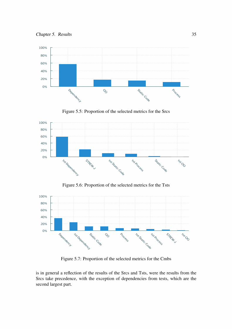
Chapter 5. Results 35
0%
20%
40%
60%
80%
100%
Dependency
OO Static-Code
Process
Figure 5.5: Proportion of the selected metrics for the Srcs
0%
20%
40%
60%
80%
100%
tst-Dependency
STREW-J
tst-Static-Code
tst-Process
Static-Code
tst-OO
Figure 5.6: Proportion of the selected metrics for the Tsts
0%
20%
40%
60%
80%
100%
Dependency
tst-Dependency
Static-Code
OO Process
tst-Static-Code
tst-Process
STREW-J
tst-OO
Figure 5.7: Proportion of the selected metrics for the Cmbs
is in general a reflection of the results of the Srcs and Tsts, were the results from theSrcs take precedence, with the exception of dependencies from tests, which are thesecond largest part.
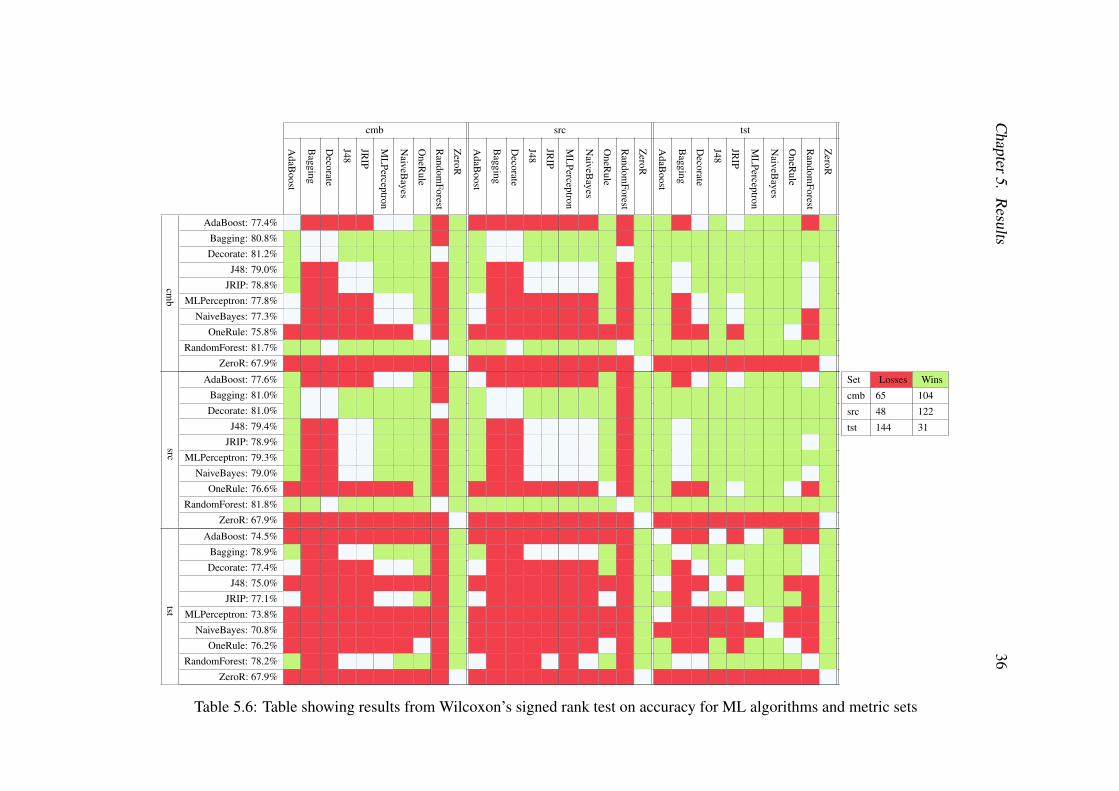
Chapter5.
Results
36cmb src tst
AdaB
oost
Bagging
Decorate
J48
JRIP
ML
Perceptron
NaiveB
ayes
OneR
ule
Random
Forest
ZeroR
AdaB
oost
Bagging
Decorate
J48
JRIP
ML
Perceptron
NaiveB
ayes
OneR
ule
Random
Forest
ZeroR
AdaB
oost
Bagging
Decorate
J48
JRIP
ML
Perceptron
NaiveB
ayes
OneR
ule
Random
Forest
ZeroR
cmb
AdaBoost: 77.4%
Bagging: 80.8%
Decorate: 81.2%
J48: 79.0%
JRIP: 78.8%
MLPerceptron: 77.8%
NaiveBayes: 77.3%
OneRule: 75.8%
RandomForest: 81.7%
ZeroR: 67.9%
src
AdaBoost: 77.6%
Bagging: 81.0%
Decorate: 81.0%
J48: 79.4%
JRIP: 78.9%
MLPerceptron: 79.3%
NaiveBayes: 79.0%
OneRule: 76.6%
RandomForest: 81.8%
ZeroR: 67.9%
tst
AdaBoost: 74.5%
Bagging: 78.9%
Decorate: 77.4%
J48: 75.0%
JRIP: 77.1%
MLPerceptron: 73.8%
NaiveBayes: 70.8%
OneRule: 76.2%
RandomForest: 78.2%
ZeroR: 67.9%
Set Losses Wins
cmb 65 104
src 48 122
tst 144 31
Table 5.6: Table showing results from Wilcoxon’s signed rank test on accuracy for ML algorithms and metric sets
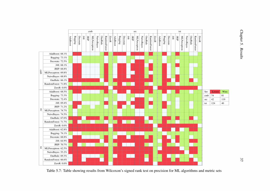
Chapter5.
Results
37cmb src tst
AdaB
oost
Bagging
Decorate
J48
JRIP
ML
Perceptron
NaiveB
ayes
OneR
ule
Random
Forest
ZeroR
AdaB
oost
Bagging
Decorate
J48
JRIP
ML
Perceptron
NaiveB
ayes
OneR
ule
Random
Forest
ZeroR
AdaB
oost
Bagging
Decorate
J48
JRIP
ML
Perceptron
NaiveB
ayes
OneR
ule
Random
Forest
ZeroR
cmb
AdaBoost: 68.1%
Bagging: 73.1%
Decorate: 72.5%
J48: 68.1%
JRIP: 68.8%
MLPerceptron: 69.8%
NaiveBayes: 68.8%
OneRule: 66.1%
RandomForest: 71.8%
ZeroR: 0.0%
src
AdaBoost: 68.5%
Bagging: 73.3%
Decorate: 72.4%
J48: 69.4%
JRIP: 71.2%
MLPerceptron: 74.7%
NaiveBayes: 74.5%
OneRule: 67.0%
RandomForest: 71.7%
ZeroR: 0.0%
tst
AdaBoost: 62.8%
Bagging: 74.1%
Decorate: 68.8%
J48: 64.9%
JRIP: 70.7%
MLPerceptron: 62.5%
NaiveBayes: 55.2%
OneRule: 69.3%
RandomForest: 66.6%
ZeroR: 0.0%
Set Losses Wins
cmb 74 81
src 42 119
tst 124 40
Table 5.7: Table showing results from Wilcoxon’s signed rank test on precision for ML algorithms and metric sets
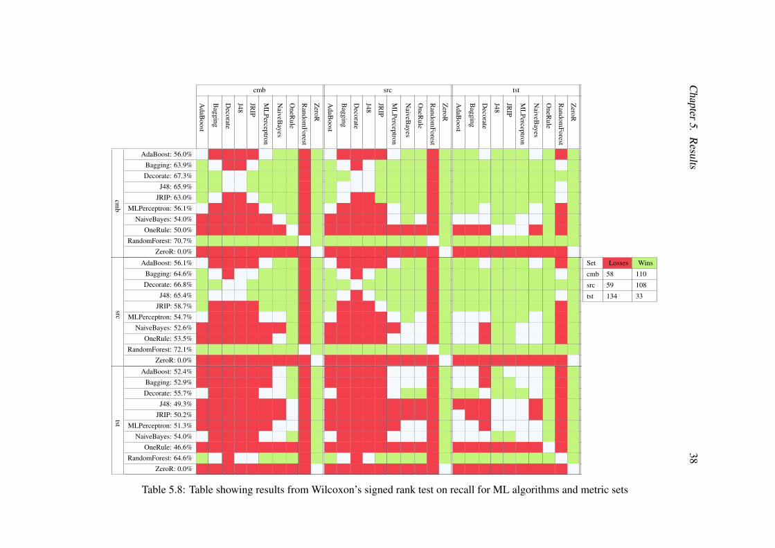
Chapter5.
Results
38cmb src tst
AdaB
oost
Bagging
Decorate
J48
JRIP
ML
Perceptron
NaiveB
ayes
OneR
ule
Random
Forest
ZeroR
AdaB
oost
Bagging
Decorate
J48
JRIP
ML
Perceptron
NaiveB
ayes
OneR
ule
Random
Forest
ZeroR
AdaB
oost
Bagging
Decorate
J48
JRIP
ML
Perceptron
NaiveB
ayes
OneR
ule
Random
Forest
ZeroR
cmb
AdaBoost: 56.0%
Bagging: 63.9%
Decorate: 67.3%
J48: 65.9%
JRIP: 63.0%
MLPerceptron: 56.1%
NaiveBayes: 54.0%
OneRule: 50.0%
RandomForest: 70.7%
ZeroR: 0.0%
src
AdaBoost: 56.1%
Bagging: 64.6%
Decorate: 66.8%
J48: 65.4%
JRIP: 58.7%
MLPerceptron: 54.7%
NaiveBayes: 52.6%
OneRule: 53.5%
RandomForest: 72.1%
ZeroR: 0.0%
tst
AdaBoost: 52.4%
Bagging: 52.9%
Decorate: 55.7%
J48: 49.3%
JRIP: 50.2%
MLPerceptron: 51.3%
NaiveBayes: 54.0%
OneRule: 46.6%
RandomForest: 64.6%
ZeroR: 0.0%
Set Losses Wins
cmb 58 110
src 59 108
tst 134 33
Table 5.8: Table showing results from Wilcoxon’s signed rank test on recall for ML algorithms and metric sets
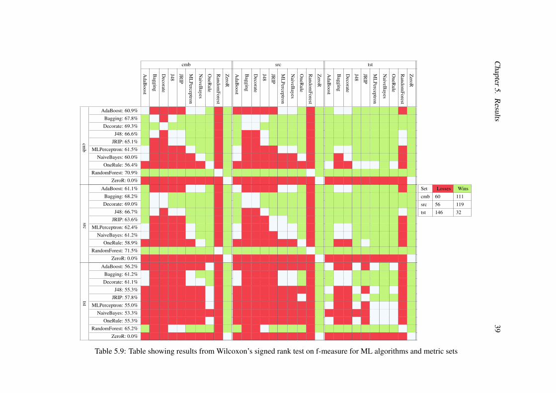
Chapter5.
Results
39cmb src tst
AdaB
oost
Bagging
Decorate
J48
JRIP
ML
Perceptron
NaiveB
ayes
OneR
ule
Random
Forest
ZeroR
AdaB
oost
Bagging
Decorate
J48
JRIP
ML
Perceptron
NaiveB
ayes
OneR
ule
Random
Forest
ZeroR
AdaB
oost
Bagging
Decorate
J48
JRIP
ML
Perceptron
NaiveB
ayes
OneR
ule
Random
Forest
ZeroR
cmb
AdaBoost: 60.9%
Bagging: 67.8%
Decorate: 69.3%
J48: 66.6%
JRIP: 65.1%
MLPerceptron: 61.5%
NaiveBayes: 60.0%
OneRule: 56.4%
RandomForest: 70.9%
ZeroR: 0.0%
src
AdaBoost: 61.1%
Bagging: 68.2%
Decorate: 69.0%
J48: 66.7%
JRIP: 63.6%
MLPerceptron: 62.4%
NaiveBayes: 61.2%
OneRule: 58.9%
RandomForest: 71.5%
ZeroR: 0.0%
tst
AdaBoost: 56.2%
Bagging: 61.2%
Decorate: 61.1%
J48: 55.3%
JRIP: 57.8%
MLPerceptron: 55.0%
NaiveBayes: 53.3%
OneRule: 55.3%
RandomForest: 65.2%
ZeroR: 0.0%
Set Losses Wins
cmb 60 111
src 56 119
tst 146 32
Table 5.9: Table showing results from Wilcoxon’s signed rank test on f-measure for ML algorithms and metric sets

Chapter 6Analysis and discussion
When looking at all algorithms the general result is that Srcs performs best. In someinstances, e.g. for recall, Cmbs performs better. At the individual results level, whenlooking at results from the metric sets and algorithms, the general result is that RandomForest works best throughout all metric sets. However, different metric sets and algo-rithms may work better in some circumstances. These results are discussed in moredetail in the following sections.
6.1 Metric sets resultsGenerally, the Srcs perform best throughout the performance measures. The only mea-sure where Srcs is not best is in recall where Cmbs in most cases is as good as Scrs andfor a few ML algorithms a little better than Srcs. As the recall denotes how good themetric set together with the algorithm is at capturing faulty files, the lower precisionfor the Cmbs may not come as a surprise. As it is capturing more faulty files, a naturalconsequence may be that it also catches more unfaulty files and therefore has a lowerprecision. This is seen in the f-measure, the combination of recall and precision, wherethe Cmbs and Srcs perform very close to each other as the results from the precisionand recall is cancelling each other out. When looking at the f-measure, one can seethat the Cmbs has a lower spread, though. The Tsts fares worse overall in all mea-sures compared to Srcs and Cmbs, but not by a very large margin. In general, one mayconclude that when choosing between the Cmbs and the Srcs, the preferred predictionperformance measure must be taken into account. If recall is of high importance, theCmbs is the metric set of choice. If precision or accuracy is most important, the Srcsis the metric set to choose.
The difference in prediction performance between Cmbs and Srcs could be due tothe feature selection process. Using a feature selected subset, can in some cases resultin lower prediction performance [45].
SrcRaw is the metric set that would have been used in case the tests were not in-cluded in the experiment and is therefore included as a reference. It generally performsworse compared to the other sets and all of the performance measures are lower thanthe Srcs, Tsts and Cmbs scores. One interesting aspect of the results is that the Tstsperforms better than srcRaw. This clearly shows that models built with metrics from
40
Chapter 6. Analysis and discussion 41
the tests, that does not have any information about the source file whatsoever, still pre-dicts better than model built with metrics from the source code itself. However, thisonly holds true for tested source code file for the Tsts and all source code files for thesrcRaw set. It must also be noted that if the same underlying dataset is used, sourcemetrics still predicts better. This could be an indicator that tested code is easier to pre-dict. This would explain the big difference between the Srcs and srcRaw which bothshare the same metric sets but use different data sets.
6.2 ML algorithm resultsThe best performing algorithm overall is Random Forest which is clearly seen in thetop three algorithms tables in 5. Generally, the best performing metric set for thealgorithms is the Srcs. There are however some cases where the best set is the Tstsfor certain algorithms, e.g. Bagging and JRip in precision. One of the benefits of JRipis the ease of which rules can be extracted and interpreted from a model built with it.The JRip result is therefore especially interesting for Ericsson, as they are interested inmodels that they can understand and interpret easily.
The Tsts set does not have as clear results as the other metric sets. Bagging comesup as one of the best algorithms for the Tsts multiple times but has especially bad recall.In turn, the precision is high, however. This is also true for the Multilayer Perceptronalgorithm for the Srcs for which recall is low and precision is high. In the end RandomForest is still the winner which the f-measure shows for both of Srsc and Tsts.
6.3 Comparison to other studiesThe comparison in Section 5.5 showed that the results of this study are comparable tothose of other studies. It also showed that the Tsts set is comparable with slightly lowerresults when compared to other studies. When looking at feature selection studies itis hard to position this study as results differ largely between them. This study doeshowever perform well when compared to Arisholm et al. which also uses a proprietarydataset. Arisholm et al. e.g. had a highly unbalanced data set with only 0.5-2% faultyfiles indicating a balance of 98%-2% which could explain their low results in othermeasures than accuracy [2, 22].
6.4 Hypothesis testing resultsTo test the null hypothesis “Source code metrics together with test metrics provideequal prediction performance as SDP using only source code metrics”, a chi-squared(χ2) test was conducted. The wins, draws and losses for Srcs and Cmbs against eachother, for each of the performance measures, were calculated and used as input tothe χ2 test. The significance level was set to α = 0.05, indicating a 95% confidence

Chapter 6. Analysis and discussion 42
interval. For accuracy, recall and f-measure, the null hypothesis could not be rejected,while for precision the null hypothesis could in fact be rejected, indicating that thereis in fact a difference in prediction performance. By performing a manual inspectionof the wins, draw and losses for prediction, it is clear that the Srcs outperforms Cmbs.This means that the hypothesis “Source code metrics together with test metrics providebetter prediction performance than SDP using only source code metrics”, stated inSection 3.2.2, does not hold.
6.5 Answers to research questions 2 and 3The research questions associated with the literature study were answered in the methodchapter, Section 3.1.5, and they are therefore not discussed further in this section. Thetwo last questions, however, were answered through the experiment and are discussedbelow.
RQ2 - Which ML algorithm(s) provide the best SDP performance?
As seen in the discussion above, Random Forest generally gives the best predictiveperformance for all the metric sets, with a few exceptions. Notably precision for allmetric sets, and accuracy for Bagging in conjunction with the Tsts. As there is nooverall winner, one has to choose a combination of metric set and algorithm that suitthe needs. In general, one may conclude that Random Forest is suitable in most cases.
6.6 Answers to research questions 4 and 5The research questions associated with the literature study were answered in the methodchapter, Section 3.1.5, and they are therefore not discussed further in this section. Thetwo last questions, however, were answered through the experiment and are discussedbelow.
RQ4 – Which ML algorithm(s) provide the best SDP performance?
As seen in the discussion above, Random Forest generally gives the best predictiveperformance for all the metric sets, with a few exceptions. Notably precision for allmetric sets, and accuracy for Bagging in conjunction with the Tsts. As there is nooverall winner, one has to choose a combination of metric set and algorithm that suitthe needs. In general, one may conclude that Random Forest is suitable in most cases.
RQ5 – To what extent do test metrics impact the performance of SDP?
For most algorithms, recall is as high, or slightly higher for the Cmbs when comparedto the Srcs metric set. Regarding the other performance measures, the Cmbs achieve

Chapter 6. Analysis and discussion 43
slightly worse results compared to the Srcs. This results in an f-measure with a compa-rable median value for the Cmbs when compared to the Srcs, but with a lower variance.One could therefore expect results closer to median value for future predictions. Whenlooking only at Tsts, the performance is generally worse than for the other sets, with afew exceptions. In conclusion, test metrics does not affect the SDP performance muchbut can give results closer to the estimated results due to its lower variance.
6.7 What the results means to EricssonFrom Ericsson’s perspective, the result of JRip in combination with Cmbs shows themost promising results as, in addition to fault predictions, rules can be extracted whichcan be used throughout the software development process.
The results produced by the tool developed through the experiment implementationcan be used in a numerous ways. First off, early estimation of what files that aremore fault prone can be predicted with good prediction performance. As describedin Chapter 1, finding faults in late stages of the development, or even in the releasedproduct is expensive. The results can therefore be used to find faults before they arereported through a TR by doing a code review on files predicted as faulty. If a fault isdiscovered through code review of files predicted as faulty, the cost of correcting thefaults is reduced. Furthermore, the time used to debug a fault reported through a TR toa certain file is eliminated if a fault is discovered through code inspection.
When using a rule based learner, the results from the tool can be used in refactor-ing1. The inspected file’s metrics can be analyzed against the rules to see why the fileis predicted as faulty. This information can then be used to refactor the file, e.g. splitthe file into smaller, cohesive units if the rule states that files with high complexity andlack of cohesion are predicted as faulty.
Rules regarding dependencies can also be used in the refactoring process. If a rulestates that a dependency causes files to be faulty, this might indicate that the depen-dency’s external interface needs refactoring. Another consideration may be to refactorfiles using a dependency and remove the dependency where possible. This would limitthe number of files using the dependency and its external interface.
The testing might also be improved as the testing effort can focus on files whichhave been predicted as faulty. Extracted rules predicting on dependencies may alsobe used where tests of files using the dependency, even if not predicted faulty, can beimproved.
Another avenue is software development process improvements. Changes in e.g.team size or configuration management2 can be evaluated in an early stage by analyz-ing changes in the predicted amount of faulty files. Again, analyzing changes in the
1“A change made to the internal structure of the software to make it easier to understand and cheaperto modify without changing its oberservable behavior” [19, p. 53]
2“The practice of identifying project artifacts and handling changes systematically so that a s systemcan maintain its integrity over time” [29, p. 664]

Chapter 6. Analysis and discussion 44
resulting rules when using a rule based learner might also give hints of how changesin the development process affect the source code and its tests. The tool is not limitedto predicting faults but can also be used to predict on any metric. The characteris-tics of files with high complexity may, for example, be further examined when usingcomplexity as the dependent variable instead of fault history.
The results of the defect prediction might also be used to prioritize tests and decidewhich tests to run when all tests can not be run due to execution time constraints. Inthis case, the tests to the files predicted as faulty, can be prioritized so that they arerun. Resulting rules containing dependencies from rule based learners may also beused. Tests of files having dependencies that often causes other files to fail, can beprioritized even if that file is not predicted as faulty.
When using a classifier where metrics from a built model can be extracted, integrityissues can emerge. Author metrics may be extracted and e.g. used for ill-intentionedpurposes. If the model is publicized, dependency metrics may be used to gain informa-tion about the repository’s structure. Due to this, the tool supports turning off certainmetric families.
When applying the tool in a production setting the model does not have to be re-built 100 times (10 folds, 10 times) as in the case of this study. The 4 days stated inChapter 5 is therefore not a measure of the performance of such a tool in a productionenvironment, rather 1 hour as only a single model needs to be built. Furthermore, a too,such as this only has to be rerun to rebuild the model after a substantial change in thecodebase, e.g. once every release. The runtime of the tool is therefore not a problemin a production setting.
6.8 Lessons learnedThe memory model first used in the experiment implementation was memory consum-ing. The usage of hash maps to record metrics, albeit both simple and flexible, turnedout to use 10 times more memory than necessary. They were however simplifyingimplementation to a large extent as metrics could be easily be added during runtime.Metrics could therefore be created on the fly based on the repository data. This fea-ture was used extensively with the dependency and author metrics. The memory usagebecame a problem when the dependency and author metrics were used on repositorieslarger than 20 000 LOC though where the number of metrics were for some reposito-ries as large as 7 000. In these cases, the memory consumption exceeded 8GB whichwas the amount of installed RAM of the computers used for the experiment. This wasdue to the number of dependency and author metrics being based on the amount ofauthors and dependencies within the repository.
The hash maps were replaced with a backend using SoA3 hosting several frontendsimplementing Java’s Map interface. The transition from a hash map based memory lay-
3Structure of Arrays. see [13, p.4-21 ]

Chapter 6. Analysis and discussion 45
out to a SoA one was therefore smooth as the Java HashMap could simply be swappedto our own implementation. The lesson one may draw from this is that the memorylayout is of importance when using metrics generated per repository as it can growlarge quite fast and being able to accommodate for this is important.
The first time results were produced by the experiment, they were extremely good,with an accuracy, precision and recall of above 95% for several ML algorithms and theCmbs. This result were not in line with other studies and the experiment design weretherefore reviewed to make sure that the results were fair. This result turned out to betoo good to be true since the feature selection was conducted in a way that made thefeature selection process using information from the test set when reducing features.This skewed the results. This problem have been present in former studies using featureselection [45, 51]. This problem was mitigated by performing feature selection on thetraining set only as proposed by Smialowski et al. [51].
After discussing the problem with an engineer it was revealed that some developersconstructs tests after a TR has been reported to stop similar faults in the future. Themere presence of a test could therefore imply that the file has had faults in the past.This problem was mitigated by applying a pivot point as described in Section 3.2. Thelesson learned by this is to be critical towards the experiment design if results are not inline with state of the art research. There may also be processes among the developerswhich are not official policy that may bias the results. It is therefore of importance totalk to developers and engineers so that the results of the experiment are not affectedby processes such as the one mentioned above.

Chapter 7Conclusion and Future Work
7.1 ConclusionThe goal of the thesis was to investigate whether a test, coupled to a source codefile, contained enough information to enhance the SDP performance if metrics fromboth the source file and test file are combined. To investigate this a literature reviewfollowed by an experiment was conducted. The literature review helped us identify ofwhat kind of metrics and ML algorithms to use in the experiment, while the experimentultimately helped us test the hypotheses.
The results of this study show that the use of Cmbs instead of Srcs does not providebetter prediction performance. In fact, in the case of precision, Srcs performs signifi-cantly better compared to Cmbs. However, the Cmbs produces less fluctuating resultsin most cases, indicating that the mean value of the evaluated prediction models arecloser to the real result, i.e. the prediction on unseen files, when using the Cmbs. Thisis visualized in the box-whisker plots in Chapter 5, where the Cmbs boxes (indicating50% of the results) are smaller in most cases, than the corresponding boxes for theSrcs.
In general, the results of our study are comparable, and in some cases better, com-pared to other similar SDP studies.
For Ericsson, this means that faults can be predicted on the file level with goodprediction performance. Perhaps the most promising result is that of the combinationof Cmbs and JRip, which makes the prediction model easy to interpret. Rules extractedfrom the model can then e.g. be used for identification of areas in need of refactoring.Conclusions drawn from these rules can also be used for e.g. process improvements.
If all of the source code files were used in the metric extraction, as they would havebeen if test metrics was not included in the prediction, the Srcs models would performconsiderably worse. This is obvious when looking at the srcRaw dataset in the figuresin Chapter 5. This shows that files with tested code, in this repository, are more likelyto be predicted correctly.
One of the most interesting results is the fact that the Tsts predicts so well havingminimal information about the source code file. This clearly demonstrates that test andsource code are tightly linked which was one of the main reasons that we thought thatcombining test and source code metrics was a viable approach.
46
Chapter 7. Conclusion and Future Work 47
One must however remark that the results of this study come from a single repos-itory and they can therefore not be claimed to be true for all source code. One canhowever argue that they likely are true for similar repositories.
7.2 Future workAs this master thesis is about determining the performance of the metric sets, onlythe default settings in the Weka environment were evaluated. As a future work, itwould be interesting to investigate how the prediction performance of different MLalgorithms could shift the results if the settings were tweaked. Hall et al. concludedthat studies with good prediction performance often have optimized their ML algorithmsettings [22]. It would be especially interesting to tweak the meta-learners used inthis master thesis, i.e. AdaBoost, Bagging and Decorate, and use different modelingtechniques together with them as they are dependent on other ML algorithms to makepredictions.
Fault Slip Through (FST), introduced by Damm et al. [14], is a measure of the costsassociated with not finding faults in the right testing phase. FST is about “to find theright faults in the right phase” [16] of the development process. This is interestingbecause not all faults can be or, perhaps should not be found with unit tests, but ratherwith e.g. integration testing, function tests or system tests. FST could be integratedinto the prediction models, where only the faults in files that could have been foundwith unit tests, i.e. errors in the source code, are the files that are considered as faulty.It would also be interesting to investigate how a FST measure, telling the model when itis most cost-effective to find the fault, could affect the predictions. There are howeverobstacles regarding the integration of FST. For example, it has to be determined in astructured way, exactly in which phase each fault should have been found which canprove to be a difficult task as the bug reporting process has to be expanded. The testeror developer filing the bug report also has to guess where the bug should have beendetected which also introduces the human factor.
One way of continuing the work of this master thesis is to include additional testsother than unit test, e.g. system tests and functional tests. The concept of FST couldthen also be utilized even further.
The term Change Bursts, described by Nagappan et al. [40] as code modules thatare frequently altered. By detecting these modules, they gained a precision and recallof 91% and 92%, respectively. Integration of this metric can therefore be recommendedas an addition to this master thesis. By using change bursts metric, the predictive powerof the models in this study could possibly be improved.
The results from this study could be validated by repeating the study for morerepositories from several other departments, conducting the same experiment on themand then comparing the results to those of this study. By doing this, the results pre-sented in this master thesis can be compared to results from repositories in relateddomains. The results from this comparison can then be used to state whether the re-

Chapter 7. Conclusion and Future Work 48
sults from this study holds true for other repositories and thereby also if the results holdtrue in general.
Another way to build on this work would be to conduct a case study to observethe impact that the tool suite has in real settings in production. The real cost savingpotential that the suite can pose to Ericsson could then be evaluated. The impact andcost savings of this tool could e.g. be measured with FST.
The tool suite could also benefit from being tested against metrics from publiclyavailable data corpus, such as the Eclipse and NASA datasets. This would possiblybe the only fair way to evaluate the prediction performance of the tool against otherstudies results since the results are highly dependent on the underlying data, and that itis a delicate problem to generalize between two different projects.

List of abbreviations
BLOC Blank LOCCA Afferent couplingsCBO Coupling Between ObjectsCCN Cyclomatic Complexity NumberCFS Correlation based Feature SelectionCK Chidamber-KemererCLOC Comment LOCCmbs Combined metric setDIT Depth of Inheterence TreeFST Fault Slip ThroughLCOM Lack of Cohesion in MethodsLOC Lines Of CodeLRP Literature Review ProtocolML Machine LearningNOC Number Of ChildrenNPM Number of Public MethodsOO Object-OrientedPD Probability of DetectionPF Probability of False alarmsRFC Response For ClassSCM Source Code Management systemSDP Software Defect PredictionSLOC Source LOCSLOC-L Logical SLOCSLOC-P Physical SLOCSLR Systematic Literature ReviewSTREW Software Testing and Reliability Early WarningSTREW-J STREW for JavaSrcs Source code metric setTR Trouble ReportTsts Test source code metric setUCC Unified Code CountWMC Weighted Methods per ClasssrcRaw The original full set of metrics for all source files
49
References
[1] Erik Arisholm, Lionel C. Briand, and Magnus Fuglerud. Data Mining Techniquesfor Building Fault-proneness Models in Telecom Java Software. In The 18th IEEEInternational Symposium on Software Reliability (ISSRE ’07), pages 215–224.IEEE, November 2007.
[2] Erik Arisholm, Lionel C. Briand, and Eivind B. Johannessen. A systematic andcomprehensive investigation of methods to build and evaluate fault predictionmodels. Journal of Systems and Software, 83(1):2–17, January 2010.
[3] S Bibi, G Tsoumakas, I Stamelos, and I. Vlahvas. Software Defect PredictionUsing Regression via Classification. In IEEE International Conference on Com-puter Systems and Applications, 2006., pages 330–336. IEEE, 2006.
[4] Barry W. Boehm. Software Engineering Economics. Prentice Hall; 1 edition,1981.
[5] Leo Breiman. Bagging predictors. Machine learning, 140:123–140, 1996.
[6] Bora Caglayan, Ayse Bener, and Stefan Koch. Merits of using repository met-rics in defect prediction for open source projects. In 2009 ICSE Workshop onEmerging Trends in Free/Libre/Open Source Software Research and Develop-ment, pages 31–36. IEEE, May 2009.
[7] Cagatay Catal. Software fault prediction: A literature review and current trends.Expert Systems with Applications, 38(4):4626–4636, April 2011.
[8] Cagatay Catal and Banu Diri. A systematic review of software fault predictionstudies. Expert Systems with Applications, 36(4):7346–7354, May 2009.
[9] Cagatay Catal and Banu Diri. Investigating the effect of dataset size, metrics sets,and feature selection techniques on software fault prediction problem. Informa-tion Sciences, 179(8):1040–1058, March 2009.
[10] S.R. Chidamber and C.F. Kemerer. A metrics suite for object oriented design.IEEE Transactions on Software Engineering, 20(6):476–493, June 1994.
[11] William W. Cohen. Fast Effective Rule Induction. In In Proceedings of theTwelfth International Conference on Machine Learning, pages 115—-123, 1995.
50
References 51
[12] James S. Collofello and Scott N. Woodfield. Evaluating the effectiveness ofreliability-assurance techniques. Journal of Systems and Software, 9(3):191–195,March 1989.
[13] Intel Corporation. Intel 64 and IA-32 Architectures Optimization Reference Man-ual. Technical Report March, 2014.
[14] Lars-Ola Damm, Lars Lundberg, and Claes Wohlin. Faults-slip-through—a con-cept for measuring the efficiency of the test process. Software Process: Improve-ment and Practice, 11(1):47–59, January 2006.
[15] Janez Dem\v{s}ar. Statistical Comparisons of Classifiers over Multiple DataSets. Journal ofMachine Learning Research, 7(12/1/2006):1–30, 2006.
[16] Denis Duka and Lovre Hribar. Fault Slip Through Measurement in SoftwareDevelopment Process. In ELMAR, 2010 PROCEEDINGS, number September,pages 177—-182. IEEE, 2010.
[17] N.E. Fenton and Martin Neil. A critique of software defect prediction models.IEEE Transactions on Software Engineering, 25(5):675–689, 1999.
[18] Norman E. Fenton and Shari Lawrence Pfleeger. Software Metrics: A Rigorousand Practical Approach. January 1998.
[19] Martin Fowler. Refactoring: improving the design of existing code. July 1999.
[20] Mark A. Hall. Correlation-based feature selection for machine learning. PhDthesis, The University of Waikato, New Zeeland, 1999.
[21] Mark A. Hall. Correlation-based Feature Selection for Discrete and NumericClass Machine Learning. 2000.
[22] Tracy Hall, Sarah Beecham, David Bowes, David Gray, and Steve Counsell. ASystematic Literature Review on Fault Prediction Performance in Software Engi-neering. IEEE Transactions on Software Engineering, 38(6):1276–1304, Novem-ber 2012.
[23] IEEE Computer Society. IEEE Standard Glossary of Software Engineering Ter-minology. IEEE Std 610.12-1990, 121990(Dec):1–84, 1990.
[24] Nathalie Japkowicz and Mohak Shah. Evaluating Learning Algorithms: A Clas-sification Perspective. Cambridge University Press, New York, New York, USA,2011.
[25] TM Khoshgoftaar, X Yuan, and EB Allen. Uncertain classification of fault-pronesoftware modules. Empirical Software Engineering, pages 297–318, 2002.
References 52
[26] Yan Ma, L Guo, and B Cukic. A statistical framework for the prediction of fault-proneness. Advances in machine learning application . . . , pages 1–26, 2006.
[27] A Mahaweerawat. Fault prediction in object-oriented software using neural net-work techniques. Advanced Virtual and . . . , 49(5):483–492, December 2004.
[28] Thomas J Mccabe. A Complexity Measure. (4):308–320, 1976.
[29] Steve McConnell. Code Complete: A Practical Handbook of Software Construc-tion, Second Edition. Microsoft Press, 2004.
[30] Prem Melville and Raymond J. Mooney. Creating diversity in ensembles usingartificial data. Information Fusion, 6(1):99–111, March 2005.
[31] Tim Menzies, Jeremy Greenwald, and Art Frank. Data Mining Static Code At-tributes to Learn Defect Predictors. IEEE Transactions on Software Engineering,33(1):2–13, January 2007.
[32] Raimund Moser, Witold Pedrycz, and Giancarlo Succi. A comparative analysis ofthe efficiency of change metrics and static code attributes for defect prediction. InProceedings of the 13th international conference on Software engineering - ICSE’08, page 181, New York, New York, USA, 2008. ACM Press.
[33] Glenford J. Myers, Corey Sandler, and Tom Badgett. The Art of Software Testing.Wiley, 2011.
[34] N. Nagappan and T. Ball. Use of relative code churn measures to predict sys-tem defect density. In Proceedings. 27th International Conference on SoftwareEngineering, 2005. ICSE 2005., pages 284–292. IEEe, 2005.
[35] Nachiappan Nagappan. Using In-Process Testing Metrics to Estimate SoftwareReliability: A Feasibility Study. . . . Software Reliability . . . , pages 1–3, 2004.
[36] Nachiappan Nagappan. A Software Testing and Reliability Early Warning (Strew)Metric Suite. PhD thesis, North Carolina State University, 2005.
[37] Nachiappan Nagappan, Thomas Ball, and Andreas Zeller. Mining metrics topredict component failures. In Proceeding of the 28th international conferenceon Software engineering - ICSE ’06, page 452, New York, New York, USA, 2006.ACM Press.
[38] Nachiappan Nagappan, Laurie Williams, Mladen Vouk, and Jason Osborne. Earlyestimation of software quality using in-process testing metrics. In Proceedings ofthe third workshop on Software quality - 3-WoSQ, page 1, New York, New York,USA, 2005. ACM Press.
References 53
[39] Nachiappan Nagappan, Laurie Williams, Mladen Vouk, and Jason Osborne. Us-ing In-Process Testing Metrics to Estimate Post-Release Field Quality. In The18th IEEE International Symposium on Software Reliability (ISSRE ’07), pages209–214. IEEE, November 2007.
[40] Nachiappan Nagappan, Andreas Zeller, Thomas Zimmermann, Kim Herzig, andBrendan Murphy. Change Bursts as Defect Predictors. In 2010 IEEE 21st Inter-national Symposium on Software Reliability Engineering, pages 309–318. IEEE,November 2010.
[41] Vu Nguyen, Sophia Deeds-Rubin, Thomas Tan, and Barry Boehm. A SLOCCounting Standard. Technical report, 2007.
[42] Thomas J Ostrand, Elaine J Weyuker, and Robert M Bell. Where the bugs are.ACM SIGSOFT Software Engineering Notes, 29(4):86, July 2004.
[43] J. Ross Quinlan. C4.5: Programs for Machine Learning. 1993.
[44] Danijel Radjenovic, Marjan Hericko, Richard Torkar, and Aleš Živkovic. Soft-ware fault prediction metrics: A systematic literature review. Information andSoftware Technology, 55(8):1397–1418, August 2013.
[45] Juha Reunanen. A Pitfall in Determining the Optimal Feature Subset Size. In Pro-ceedings of the 4th International Workshop on Pattern Recognition in InformationSystems, pages 176–185. SciTePress - Science and and Technology Publications,2004.
[46] J. Riquelme, J. C., Ruiz, R., Rodrıguez, D., Moreno. Finding defective mod-ules from highly unbalanced datasets. Actas de los Talleres de las Jornadas deIngeniería del Software y Bases de Datos, 2(1):67–74, 2008.
[47] Adrian Schröter, Thomas Zimmermann, and Andreas Zeller. Predicting compo-nent failures at design time. In Proceedings of the 2006 ACM/IEEE internationalsymposium on International symposium on empirical software engineering - IS-ESE ’06, page 18, New York, New York, USA, 2006. ACM Press.
[48] Sana Shafi, Syed Muhammad Hassan, Afsah Arshaq, Malik Jahan Khan, andShafay Shamail. Software quality prediction techniques: A comparative analysis.In 2008 4th International Conference on Emerging Technologies, pages 242–246.IEEE, October 2008.
[49] Shivkumar Shivaji, E. James Whitehead Jr., Ram Akella, and Sunghun Kim. Re-ducing Features to Improve Bug Prediction. In 2009 IEEE/ACM InternationalConference on Automated Software Engineering, number Section II, pages 600–604. IEEE, November 2009.
References 54
[50] Forrest Shull, Vic Basili, Barry Boehm, A.W. Brown, Patricia Costa, MikaelLindvall, Dan Port, Ioana Rus, Roseanne Tesoriero, and Marvin Zelkowitz. Whatwe have learned about fighting defects. In Proceedings Eighth IEEE Symposiumon Software Metrics, pages 249–258. IEEE Comput. Soc, 2002.
[51] Pawel Smialowski, Dmitrij Frishman, and Stefan Kramer. Pitfalls of super-vised feature selection. Bioinformatics (Oxford, England), 26(3):440–3, February2010.
[52] D. Spinellis. Tool Writing: A Forgotten Art? IEEE Software, 22(4):9–11, July2005.
[53] Burak Turhan and Ayse Bener. Analysis of Naive Bayes’ assumptions on softwarefault data: An empirical study. Data & Knowledge Engineering, 68(2):278–290,February 2009.
[54] Burak Turhan, Tim Menzies, Ayse B. Bener, and Justin Di Stefano. On the rela-tive value of cross-company and within-company data for defect prediction. Em-pirical Software Engineering, 14(5):540–578, January 2009.
[55] Frank Wilcoxon. Individual Comparisons by Ranking Methods. Biometrics Bul-letin, 1(6):80, December 1945.
[56] Ian H. Witten, Eibe Frank, and Mark A. Hall. Data Mining: Practical MachineLearning Tools and Techniques, Third Edition (The Morgan Kaufmann Series inData Management Systems). Morgan Kaufmann, 2011.
[57] He Zhang, Muhammad Ali Babar, and Paolo Tell. Identifying relevant studiesin software engineering. Information and Software Technology, 53(6):625–637,June 2011.
[58] Hongyu Zhang. An investigation of the relationships between lines of code anddefects. In 2009 IEEE International Conference on Software Maintenance, pages274–283. IEEE, September 2009.
[59] Hongyu Zhang and Xiuzhen Zhang. Comments on "Data Mining Static CodeAttributes to Learn Defect Predictors". IEEE Transactions on Software Engi-neering, 33(9):635–637, September 2007.