Soft Information in

Earnings Announcements:

News or Noise?

_______________

Elizabeth DEMERS

Clara VEGA

2010/33/AC

(Revised version of 2008/44/AC/FIN)

Soft Information in Earnings Announcements: News or Noise?*

May 2010

By

Elizabeth Demers**

and

Clara Vega***

Revised version of 2008/44/AC/FIN

* We thank Cam Harvey, two anonymous referees and an anonymous associate editor for their very valuable comments. We also thank workshop and conference participants at the Federal Reserve Board of Governors, Duke University, Lancaster University, the Swiss Finance Institute in Lugano, the University of Barcelona, the University of Fribourg, the National University of Singapore, the European Accounting Association and American Accounting Association annual meetings, the Conference on Forensic Accounting, Internal Control, and Corporate Governance at the University of Toronto, the Society for Economic Dynamics Istanbul 2009 meeting, in addition to Dan Givoly, Stuart McLeay, Per Olsson, Katherine Schipper, Steve Sharpe, Jeremy Stein, and especially Jennifer Francis for valuable comments and discussions. We also appreciate the excellent research assistance of Armel Allard, Monique Bruet, Shannon Demers, Nicholas Klagge, Marcus Newman, and Hien Tran, we thank Craig Carroll for processing our text files using the Diction software, and we thank PR Newswire for providing us with the earnings announcement data. The views presented in this paper are solely those of the authors and do not represent the views of the Federal Reserve Board or its staff.

** Assistant Professor of Accounting & Control at INSEAD, Boulevard de Constance, 77305 Fontainebleau Cedex, Email: liz.demers@insead.edu Tel: +33 (0)160729206

*** Board of Governors of the United States Federal Reserve System International Finance Division 20th

Street & Constitution Avenue, NW Washington, DC 20551 Email: clara.vega@frb.govTel: +1 202-452-2379

A working paper in the INSEAD Working Paper Series is intended as a means whereby a faculty researcher's thoughts and findings may be communicated to interested readers. The paper should be considered preliminary in nature and may require revision. Printed at INSEAD, Fontainebleau, France. Kindly do not reproduce or circulate without permission.

Abstract

This paper examines whether, and under what conditions, the “soft” information contained in the text of management’s quarterly earnings press releases is incrementally informative over company-issued “hard” information. We use several textual-analysis programs to extract various dimensions of managerial net optimism from more than 20,000 corporate earnings announcements over the period 1998 to 2006 and document that unanticipated net optimism in managers’ language affects announcement period abnormal returns and predicts post-earnings announcement drift. We further find, consistent with economic theory, that two key aspects of the information environment influence the price-responsiveness to net optimism: (i) the informativeness of the contemporaneously available hard information; and (ii) the likely credibility of the net optimism itself. We also show that the second moment of soft information, the level of uncertainty in the text, attenuates the market’s response to earnings announcement surprises, is associated with contemporaneous announcement period idiosyncratic volatility, and predicts future idiosyncratic volatility incrementally to “hard” information. JEL Classifications: G14; D82; M41 Keywords: Soft Information; Earnings Announcements; Post-earnings Drift;;Cheap Talk;Languge Tone; Earnings Quality; Information Uncertainty; Momentum; Voluntary Disclosure

2

1. Introduction

The process of price discovery in financial markets remains poorly understood.

Numerous studies show that quantitative information about fundamentals explain only a

small portion of asset price movements (e.g., Shiller (1981), Roll (1988), Mitchell and

Mulherin (1994)). In the specific context of earnings announcements, Brandt et al (2008)

suggest that considerable information in addition to bottom line earnings news arrives around

the announcement date, a significant portion of the market’s reaction around that date is

attributable to other information that managers release contemporaneously with the bottom

line earnings, and the proportion of the market’s reaction that is attributable to this

complementary information is on the rise. Thus, identifying additional sources of

fundamental information that are incorporated into asset prices, particularly at the earnings

announcement date, is of basic importance to financial economics. In this paper we analyze

one key form of data, the qualitative verbal information that managers communicate in their

quarterly earnings announcements (henceforth, “soft information”). The general finding from

our study, that the tone or sentiment of managerial language influences stock price dynamics,

may seem surprising given the voluntary and less formally constrained nature of this soft

information. However, we show that our findings are consistent with economic theory. On

an anecdotal level, the significance of our soft information language metrics also accords

with the recent surge in the use of linguistic algorithms by investment firms and with the

associated rise in the number of entities that sell such algorithmically processed data (e.g.,

Ravenpack).1

Using a novel data set consisting of over 20,000 corporate earnings announcements

filed with the PR Newswire service during the period of January 1998 through July 2006, we

characterize the response of asset prices to soft and hard information communicated by

managers in the earnings report. In particular, we use well-established linguistic algorithms

to quantify two dimensions of managerial soft information – net optimism and certainty – and

we show that, on average, soft information affects asset prices both within the earnings

announcement event window and during the 60-trading-day post-announcement period, even

after controlling for contemporaneously released hard information. We contribute to the

literature relating linguistic content to stock price dynamics by examining the influence of a

1 Language algorithms are now used by investment managers to automatically read and code press releases for the purpose of generating trading orders. The texts are being processed, and the trading orders executed, even more quickly than human analysts are able to finish reading the first line of the release (The Economist, June 21, 2007).

3

new language construct, certainty, and by showing that two key aspects of the information

environment influence the price-responsiveness to net optimism: (i) the informativeness of

the contemporaneously available hard information; and (ii) the credibility of the net optimism

itself.

We first examine the potentially complementary role of soft information in the price

formation process by documenting that it plays a heightened role in settings where hard

information provides a noisier valuation signal. Specifically, we find that net optimism is

priced more for high tech firms, for firms with high price-to-earnings (PE) ratios, for firms

with high R&D expenses, and for companies with lower quality accounting data. Firms with

these characteristics all have in common that their historical earnings realizations (and current

or near-future earnings projections) are less informative for stock valuation. The finding of

greater price responsiveness to soft information in settings where the hard information

provides a noisier measure for valuation is consistent with both standard Bayesian learning

models that do not consider soft information per se (e.g., Kim and Verrecchia (1991),

Krueger and Forston (2003), and Hautsch and Hess (2007)), as well as with models that do

explicitly consider soft information (e.g., Dye and Sridhar (2004)).

We also find evidence that is consistent with theories that highlight the importance of

the credibility of net optimism in explaining the price-responsiveness to soft information.

Although securities regulations clearly prevent executives from making factually misleading

statements about their firms, the credibility and information content of the more subtle

linguistic aspects of managerial earnings announcements are questionable because of this

information’s key features; it is difficult to verify. This characteristic of soft information in

equity markets with incomplete information is similar to the settings contemplated by “cheap

talk” theories. The central question in these models is, what truth-revealing mechanisms

allow information to be credibly transmitted when communication is ex-ante costless and

difficult to verify? In the context of our managerial earnings announcements, we find

evidence in support of three mechanisms proposed by the literature to induce truthful

revelations: the verifiability of the (soft) information; the existence of multiple informed

experts; and reputational concerns on behalf of the agent.

The cheap talk theory of Benabou and Laroque (1992) establishes the notion that

verifiability is a key mechanism for inducing truthful information revelation. In the context

of soft information, Dye and Sridhar’s (2004) model predicts that the level of managerial

manipulation of this data is decreasing in the extent to which outside observers can verify it.

In our empirical setting, we expect that one mechanism available to managers to enhance the

4

credibility of their soft information is to support it with hard data, such as voluntarily

disclosed accounting figures that are ultimately verifiable via the quarterly reporting and

annual audit requirements.2 Consistent with this, we find that the managerial net optimism in

statements containing more numerical terms (i.e., statements that provide more detailed,

precise, and verifiable hard information) impacts asset prices by 24 basis points more than

statements containing fewer numerical references.

Krishna and Morgan (2001) show that the existence of multiple experts reporting

simultaneously to the decision maker improves the informational content of soft information

conveyed by managers, even if the experts have a similar bias. We test this theory empirically

by considering the presence of analysts and journalists following the firm to be indicative of a

setting in which “multiple experts” are transmitting information.3 Consistent with theory, we

find that the net optimism of firms with high media coverage impacts asset prices by 37 basis

points more than that of firms with low media coverage and the net optimism of firms with

high analyst coverage impacts asset prices by 35 basis points more than that of firms with low

analyst coverage.

We also examine the role of reputation in enhancing the credibility of soft

information. Although there are surprisingly few “cheap talk” models that allow for the

repeated interaction of the sender and receiver of information, Sobel (1985) first considers

this mechanism and shows that the sender truthfully reveals his information because he cares

about his reputation. More directly related to our setting, Stocken (2000) models managerial

incentives to disclose privately observed non-verifiable information and predicts that credible

communication is less probable for a manager with poor reputation. Consistent with this

prediction, we find that the net optimism of firms with better management forecasting

reputations impacts asset prices by 43 basis points more than that of managers with weaker

reputations.

In terms of the second dimension of soft information, “certainty,” we test whether the

use of more versus less resolute language provides useful information regarding the precision

2 The content of the quarterly earnings announcement beyond the “bottom line” earnings figure is subject to considerable managerial discretion. In particular, the provision of detailed or decomposed earnings-related information, such as sales growth, R&D spending, divisional performance results, and so forth, is not required but may be voluntarily discussed by management. 3Krishna and Morgan (2004) show that even if the condition of multiple experts being informed is relaxed, repeated two-way communication between one informed expert (the manager) and uninformed receivers of information will improve the information content of communications. Applying this principle to our setting suggests that relaxing the assumption that analysts and journalists are informed still leads to the prediction that there is more information content in the soft information conveyed by managers of firms with higher levels of coverage.

5

of the hard and soft information conveyed by managers in their earnings statement.4

Bayesian learning models predict that the impact of a public signal on asset prices is

increasing in its own precision and decreasing in the precision of other public signals.

Accordingly, if our certainty variable measures the precision of hard (soft) information more

so than the precision of soft (hard) information, then we expect the hard (soft) information of

high certainty firms to impact asset prices more than the hard (soft) information of low

certainty firms, while we expect the soft (hard) information of high certainty firms to impact

asset prices less. Since little is known about managerial linguistic certainty in the context of

earnings announcements, which effect will dominate remains an empirical question.

We first explore the properties of linguistic “certainty” and find that it is negatively

correlated with measures of economic uncertainty commonly used in the literature, such as

earnings volatility, the inverse of the managerial earnings’ forecast precision, dispersion

across analyst forecasts, price-earnings ratios, research and development expenses, and an

indicator variable for firms being in the high tech sector. We then document that the hard

earnings surprise of more “certain” statements impacts asset prices more, although we do not

find a corresponding decrease in the impact of high certainty firm’s soft information on

prices. This finding suggests that in the cross-section of firms, the certainty characteristic

tends to modify hard information. For a subsample of firms that have noisier hard earnings

news, we confirm our expectations that the market responds more intensively to the soft

information of high certainty versus low certainty announcements. In other words, when

earnings provide a noisy signal for valuation and thus more reliance must be placed on the

soft information, managerial linguistic certainty tends to modify the market’s response to that

soft information.

Theory unambiguously predicts that the post-announcement drift of low certainty

firms should be higher than the post-announcement drift of high certainty firms. Theory also

predicts that the idiosyncratic volatility during both the announcement and post-

announcement periods should be higher for low certainty firms. Consistent with this, we find

that both the hard and soft news in the earnings announcements of low certainty firms predict

higher post-announcement drift (although the predictive ability is stronger for soft

information). We also find that the level of certainty expressed in managers’ earnings

announcements is inversely related to idiosyncratic volatility during the announcement

period, and that it is also an inverse leading indicator for post-announcement abnormal

4 We do not consider the possibility that managers strategically use more versus less resolute language because there is no theory to guide our empirical tests along this dimension.

6

volatility. Our findings of an association between uncertainty in managers’ language and the

second moment of stock returns are consistent with Bayesian learning models, and the results

are robust to controlling for fundamental measures of uncertainty in the firm’s economic

environment.

Our study contributes to the nascent literature that uses textual analysis software to

extract potentially price informative soft information from media and management

communications. Our study differs from those of Tetlock (2007), Tetlock, Saar-Tsechansky

and Macskassy (2008), and Engelberg (2008) in that all of these prior works examine the

association between media-expressed negativity and future measures of firm performance,

while we examine the relation between management-expressed sentiment and various price

metrics. Relative to the media, managers have different insights, motivations, biases,

reputations, and fiduciary duties in their communications with parties who are external to the

firm. This differential alignment of interests, together with the subtlety of the language

constructs derived from press releases, enable us to test “cheap talk” theories in the context of

managerial earnings announcements.5 We also use a much broader sample of firms that are

not all subject to the high information environments of the S&P 500 companies underlying

the previous media studies, which provides us with the cross-sectional variation necessary to

examine whether and how firm characteristics affect the market’s response to soft

information.

We add a further dimension to the literature by expanding the set of linguistic

constructs examined in the context of asset pricing dynamics. While Tetlock, et al. (2008),

Davis, Piger and Sedor (2008), Mayew and Venkatachalam (2009), and Engelberg (2008) all

examine one similar dimension of language (alternatively operationalized as either negativity,

positivity, or net optimism), we consider the role of both net optimism as well as certainty in

explaining contemporaneous and future stock returns and volatilities.6

The rest of this paper is organized as follows. Section 2 describes the theoretical

motivation for the hypotheses to be tested, and summarizes the related literature. Section 3

describes our sample, data sources, and the measurement of our soft information variables.

In Section 4 we empirically examine whether, and under what circumstances, the unexpected

component of managerial net optimism is incorporated into asset prices during each of the

5 Although Loughran and McDonald (2010), Li (2006) and Davis, Piger and Sedor (2008) also consider management-issued communications, the focus of their papers is very different from ours. We discuss and relate their findings to ours whenever appropriate. 6 Loughran and McDonald (2010) and Li (2006) also investigates the notion of certainty. We compare our measure to that of Loughran and McDonald (2010) in Section 5.

7

short-window announcement and post-announcement drift periods. Section 5 explores the

role of linguistic certainty in the price-setting processing, first by examining its modifying

effect on the news-price relation, and then by investigating its association with idiosyncratic

stock price volatilities. Section 6 provides a summary and conclusion to our study.

2. Theory and Literature

Most theories of information aggregation assume that managers release credible hard

information, while much less attention has been devoted to the questions of whether and how

soft information should be incorporated into asset prices. In what follows, we provide a

summary of the relevant theoretical literature that relates to, and motivates, our empirical

investigation of soft information’s role in the price setting process.

2.1 The Complementarity of Soft and Hard Data

Intuitively, when an investor is provided with two (or more) signals that contain

orthogonal, price-relevant information, each signal should be relied upon in the price setting

process.7 Applying this concept to our empirical setting, we expect that managerial language

in corporate earnings announcements will impact prices incrementally to the simultaneously

released hard information provided that the linguistic measures are credible (an issue

discussed at length in the subsequent section) and contain non-overlapping signals about the

firm’s future cash flows. Dye and Sridhar (2004) provide a model that formalizes this

intuition, wherein managers simultaneously release hard and soft information and they show

that in efficient markets there is a unique linear equilibrium in which prices are a linear

function of both the soft and hard information managers released. In other words, they

predict that hard and soft information should complement each other in the price setting

process, a conjecture for which prior empirical studies (e.g., Davis, et al. (2008)) provide

empirical support, and which we also confirm with our dataset.

Dye and Sridhar (2004) further show that the impact of soft information on prices is

increasing in the noise of the hard information. We empirically test this in our empirical

setting by investigating the relative response to soft information for firms with more versus

less noisy earnings, where we rely upon the prior literature’s findings to identify alternative

7 This result is also formally derived from standard Bayesian learning models in which investors observe more than one hard information signal related to the fundamental value of an asset (e.g., Kim and Verrecchia (1991), Krueger and Fortson (2003), and Hautsch and Hess (2007)).

8

subsamples of firms that are deemed to have earnings realizations that are less informative for

valuation.8

2.2 Credibility of Net Optimism

The classic “cheap talk” model of Crawford and Sobel (1982) predicts that, as long as

the interests of managers and investors are closely aligned, managers will provide useful and

credible information. Consistent with this, our tests of the complementarity theories discussed

above implicitly assume that both the soft and hard information signals received by investors

are credible. However, Crawford and Sobel (1982) and other “cheap talk” theories also

suggest that, because it is difficult for investors to verify soft information, any misalignment

of interests may cause managers to send uninformative or misleading messages.9 The “cheap

talk” literature thus examines the robustness of the “babbling” equilibrium and explores the

relevance of different truth revealing mechanisms. We consider the language characteristics

of managerial earnings announcements to bear the key characteristics of the “cheap talk”

considered in theoretical models – namely, soft information is ex-ante costless to managers

and difficult for investors to verify – and we therefore extend our investigations to test

various theories that relax the assumption of credible (soft) information conveyance.

2.2.1 Verifiability of Messages

The cheap talk theory of Benabou and Laroque (1992) reinforces the notion that

verifiability is the key to truthful revelation. In their model, managers with unfavorable

information remain silent or lie because investors are unable to distinguish honest managers

with uncertain information from dishonest managers with precise information. If messages

are verifiable, however, investors can perfectly distinguish between the two types of firms

and truthful revelation is the unique equilibrium. Dye and Sridhar’s (2004) model similarly

predicts that the level of managerial manipulation of soft information is decreasing in the

extent to which outside observers can verify the soft information. We empirically examine

the notion that verifiability influences investors’ reliance on soft information by comparing

the price response to managerial net optimism that is accompanied by more verifiable hard

8 For example, Lev and Zarowin (1999), amongst others, have documented that firms that are heavily laden with intangible assets, such as those that are R&D-intensive or otherwise classified as “high tech” or “growth” type firms have noisier historical earnings from a forward-looking valuation perspective. 9 It is the misalignment of preferences, together with the separation of ownership and management and the associated information asymmetries, that give rise to the agency problems commonly discussed in the “cheap talk” and financial reporting literatures (see Beyer, Cohen, Lys and Walther (2009) for a comprehensive review).

9

information (i.e., more numerical terms) with announcements that provide less hard support

to their soft information.

2.2.2 Multiple Informed Experts

Krishna and Morgan (2001) consider a single period model in which there is one

decision maker (i.e., an investor) together with more than one informed and interested expert.

Their model shows that when multiple experts report to the decision maker simultaneously,

the problem of truthful information revelation is solved, even if all experts have a similar

bias. We test this theory empirically by considering the presence of analysts and journalists

following the firm to be indicative of a setting in which “multiple experts” (i.e., together with

the firm’s management) are transmitting information. Our assumption is supported by, e.g.,

Core (2001) who concludes in his review of the voluntary disclosure literature that financial

analysts provide useful information, and similarly by the findings of Bushee, Core, Guay and

Hamm (2010) which suggest that the press helps to reduce information problems around

earnings announcements. We note, however, that the assumption that analysts and journalists

are informed is not necessary; Krishna and Morgan (2004) show that, even when the

condition of multiple experts being informed is relaxed, repeated two-way communication

between uninformed agents and one informed agent (such as that suggested by the interaction

of analysts and the media with management) will improve the informational content of the

soft information conveyed by managers.

2.2.3 Reputation

All of the results that we describe above derive from single period models. In

repeated games, wherein the sender and receiver of communication are allowed to

communicate more than once, the information problem has been shown to be mitigated. In

the first such model, Sobel (1985) shows that in a one-period model no communication is

revealed, while in a repeated game the sender truthfully reveals his information both because

he cares about his reputation and because the information is ex-post verifiable. More directly

related to our setting, Stocken (2000) models managerial incentives to disclose privately

observed information in a multi-period model. His theory suggests that credible

communication is less probable for a manager with a poor reputation. Stocken’s (2000)

intuition is consistent with that of Holmstrom (1999) under some narrow assumptions, but in

general Holmstrom (1999) shows that it is not necessarily the case that agents with a longer

reputational history have less incentive to lie. We empirically test the hypothesis that

10

markets respond more to the soft information of managers with better reputations using the

managerial forecasting reputation measure proposed by Hutton and Stocken (2009).

2.3 The Effect of Certainty on Asset Price Changes

Theory provides an ambiguous prediction regarding the effect of certainty in

modifying the impact of soft and hard information on asset prices. If the linguistic certainty

measure relates exclusively to the precision of hard information, then Dye and Sridhar (2004)

and standard Bayesian learning models (e.g., Kim and Verrecchia (1991), Krueger and

Fortson (2003), and Hautsch and Hess (2007)) predict that the soft information of firms with

high certainty will have a smaller impact on prices (because it is less useful as a complement

to the more certain hard information) and the hard information of such firms will have a

bigger impact on prices. Conversely, if the certainty linguistic measure solely captures the

precision of the soft information provided by the manager, then investors are expected to

place more weight on the soft information and less weight on hard information. A third

possibility is that the linguistic measure solely captures the predictability of future cash flows,

in which case these models predict that both the soft and hard information of high certainty

firms will have a smaller impact on asset prices because if future cash flows are deterministic

then information is not valuable. It remains an empirical question as to whether the certainty

in managerial language derives from inherent uncertainties in the accuracy of managers’ soft

information or hard information, or more generally from uncertainties regarding the firm’s

expected future earnings and cash flows.10 To address this issue, we first examine the

correlations between our linguistic certainty measures and various “hard information”

measures of economic uncertainty from the prior literature. We then formally test whether

the soft and hard information of firms that use higher levels of resolute language

differentially impact prices relative to those that use less precise language by interacting

certainty with the surprises in net optimism, earnings realizations, and management earnings

forecasts, respectively.

10 Another alternative possibility is that the certainty measure captures the strategic use of more versus less resolute language. In Benabou and Laroque’s (1992) model, investors cannot differentiate between a manager who is truthfully revealing his private information but observes a noisy signal of the state of the firm versus a manager who is not truthfully revealing his private information and observes a precise signal of the state of the firm. In such a set up managers who manipulate information may speak with less certainty and hence the soft information released by these managers should impact prices less. Empirically, we cannot distinguish between the case of such strategic use of more ambiguous language from a setting where the manager has less precise soft information to convey (i.e., in either case, the market’s response to the soft information is expected to be attenuated).

11

Brav and Heaton (2002), among others, predict that the information of firms that face

more uncertain environments will be incorporated into asset prices more slowly. We test this

hypothesis by comparing the post-earnings announcement drift of high certainty firms to that

of low certainty firms.

2.4 The Effect of Certainty on Asset Price Volatility

Dye and Sridhar (2004)’s theory predicts that lower levels of certainty regarding hard

or soft information, or related to expected future earnings, are all unambiguously associated

with higher levels of return volatilities during the announcement period. We test this

hypothesis by examining the association between our certainty measure and event window

asset price volatility, after controlling for volatility’s other known determinants. As a

robustness check, we also examine the predictive power of our certainty measure for post-

announcement idiosyncratic volatility.

3. Sample and Data Description

3.1 Samples We obtain the text of quarterly earnings announcements for the period of January

1998 through July 2006 from PR Newswire. We are able to match, using the ticker symbol

and the announcement date (allowing for a 3-trading-day window discrepancy), 27,705 of the

PR Newswire observations with the CRSP/Compustat database (4,771 different firms) and

18,673 of these announcements are further matched to First Call (3,433 different firms).

Hereafter we refer to these two samples as the “Compustat” and “First Call” samples,

respectively. We include only those observations for which we can calculate earnings

surprises, 3-trading-day abnormal returns surrounding the earnings announcement, and 60-

trading-day abnormal returns both prior to, and post-, announcement. We also drop

observations with stock prices below $1 and above $10,000 and firms with negative or

missing book values. We drop earnings announcement days that are within two weeks of a

dividend payment announcement or a merger and acquisition announcement, and we drop

announcements that contain less than 100 words. After imposing all of the preceding

restrictions, we are left with a final sample of 3,683 firms (2,729 firms) and 20,899 firm-

quarter (14,649 firm-quarter) observations for the Compustat (First Call) sample.

Throughout the main body of the paper, we tabulate and discuss the results of all of

our tests using only the Compustat sample, however we also tabulate the results from all of

12

the same tests using the First Call sample in Appendix A. We choose to focus on the

Compustat sample for our main tests for several reasons. First, the First Call constraint

imposes a bias in favor of the inclusion of firms that are larger and subject to richer

information environments, while we are also interested in understanding the role of soft

information for the broader universe of firms that are not subject to such high exposure and

associated media and analyst filtering mechanisms. Second, Graham, Harvey and Rajgopal

(2006) report that 85.1% of CFO survey respondents considered earnings in the same quarter

of the prior year to be the most important earnings benchmark, followed secondly by the

analyst consensus estimate at 73.5%. The CFOs interviewed in their study further noted that

the first item in their press release is often a comparison of the current quarter’s earnings with

four-quarters-lagged earnings. Accordingly, we expect that the prior year’s same quarter

actual earnings provides the framing context for management’s current earnings

announcement even if it is not the figure associated with the strongest market response for

firms that are tracked by analysts. Despite the above mentioned advantages of the Compustat

sample, however, we still feel that it is important to discuss the First Call sample results. In

particular, the First Call sample results show that our findings are robust to alternative

measures of hard earnings information and to alternative samples.

3.2 Data

We obtain market values, stock returns, and trading volume from the Center for

Research in Security Prices (CRSP) databases, while historical accounting data are obtained

from Compustat. Media counts are derived from the Factiva database. First Call is the

source for both management and analyst forecasts, however our results are robust to using

IBES analyst forecasts rather than First Call analyst forecasts, and to supplementing the First

Call analyst forecasts with IBES data where firms are covered by the latter but not by the

former database. Because only First Call provides corresponding management forecasts, we

choose to report the results that rely exclusively on this database.

Corporate quarterly earnings announcements are provided by PR Newswire, with

each firm-quarter’s announcement being furnished as an individual text file. Prior to

subjecting these files to the linguistic algorithm processing described below, we undertake a

number of analyses upon, and make a number of modifications to, the announcements. First,

we use keyword searches to develop indicator variables for the presence of an income

statement, a balance sheet, and a statement of cash flows, respectively, in each announcement

13

file. Next, we identify tabulated figures in the text (including the financial statements) by

searching for strings of numbers, and where identified we cut these elements from the files so

that tables of figures are not confounding the textual linguistic analysis.11 Third, using

mechanical search algorithms that we designed based upon extensive manual review of the

announcements, we separately remove the company description and “safe harbor” paragraphs

from the announcements so that only the earnings announcements themselves remain in the

text files to be analyzed.12

3.3 Measuring Net Optimism and Certainty

There has been an increased interest in recent years in determining the sentiment and

degree of certainty conveyed in public communications by government institutions, the

media, and corporate entities. Various methods have been employed to measure the soft

information contained in these communications and to systematically analyze its impact on

market measures of activity and individual behavior. These methods include: manual

researcher-developed classifications as in Ehrmann and Fratzscher (2007) or machine-driven

researcher-specified word counts as in Li (2006); researcher-designed automated scoring

programs as in Lucca and Trebbi (2008) or Bayesian-updating methods as in Antweiler and

Frank (2004) and Li (2008); the development of optimism (or “bullishness”) indices based

upon multiple underlying language processing algorithms as in Das, Martinez-Jerez and

Tufano (2005) and Das and Chen (2007); Diction software for the extraction of linguistic

characteristics (e.g., Bligh and Hess (2007); Ober, Zhao, Davis and Alexander (1999);

Yuthas, Rogers and Dillard (2002); and Davis, et al. (2008), amongst many others)13;

General Inquirer, an alternative linguistic algorithm (Tetlock (2007), Tetlock, et al. (2008),

and Engelberg (2008)); alternative, researcher-developed finance-oriented dictionaries for use

in language word count type programs (Loughran and McDonald (2009)); and the

development of a common word weighting scheme to reduce the potential misclassifications

11 The language algorithms typically count each numerical expression as a “word” and thus leaving numerical tables in the files will confound the measurement of the linguistic constructs that we wish to extract from the texts by exaggerating both the total number of words as well as the numerical term scores. We explicitly include other variables designed to capture the presence and/or contents of the quarterly financial statements. 12 The company description sections typically describe the entity in extremely positive terms, whereas the safe harbor provisions include many uncertainty-related expressions. Thus, their inclusion would have the effect of increasing the net optimism, positivity, and uncertainty linguistic scores in an artificial manner in the sense that neither of these sections is directly related to the managerial earnings announcement news per se that we seek to analyze. 13 See http://www.dictionsoftware.com/files/dictionresearch.pdf for a more extensive summary of published academic studies using the Diction software.

14

caused by using generic linguistic programs in the financial reporting context (Loughran and

McDonald (2009)).

To evaluate the sensitivity of our results to different measures of soft information, we

consider three different algorithms to measure the net optimism in managers’ earnings

announcements, General Inquirer (“GI”), version 6.0 of the Diction text-analysis program,

and the Loughran-McDonald dictionaries (“L&M”). We also consider a fourth alternative

measure, the first factor of these three measures of net optimism. Specifically, we use

principal components analysis to extract the orthogonal factors F(t) from the covariance

matrix of the vector, such that X(t)=A+B×F(t), where A and B are matrices of constants and

factor loadings, respectively, and X(t) is a (3×1) vector of net optimism measures. The first

factor, which loads about equally on all three measures, explains 65 percent of the variation

in these three measures and henceforth we refer to this measure as the net optimism factor.

Similarly, for certainty we use two different algorithms, version 6.0 of the Diction text-

analysis program, and the Loughran-McDonald dictionary (“L&M”), to estimate certainty

(General Inquirer does not offer a linguistic construct that is analogous to certainty) and we

also consider the first factor as an alternative measure.

In general, each of the textual analysis algorithms that we consider uses a series of

dictionaries (i.e., word-lists) to search text passages for different semantic features. For

example, Diction defines optimism as “language endorsing some person, group, concept or

event or highlighting their positive entailments” (Digitext Inc. (2000)) and the Diction

formula for net optimism is [praise + satisfaction + inspiration]-[blame + hardship + denial].14

Following prior studies, we interpret the first and second components of the optimism

formula as “optimism” and “pessimism,” respectively, and we refer to the difference between

the two as “net optimism.” We obtain analogous measures of net optimism by using

positivity minus negativity from GI, and Fin-Pos minus Fin-Neg from version 2 of the L&M

dictionaries. The measures of optimism and pessimism (or their analogues, positivity and

negativity) are stated as a percentage of the total words in the text article, which we then

multiply by 100 in order to arrive at variables that are bounded by 0 and 100. Net optimism,

being the difference between optimism and pessimism (or positivity and negativity), is thus

bounded by -100 and 100.

Diction defines certainty as, “language indicating resoluteness, inflexibility, and

completeness and a tendency to speak ex cathedra” (Digitext Inc. (2000)), and the Diction

14 The terms associated with each of the characteristics that generate the Diction variables are reproduced in Davis, et al. (2008) and are available in extended detail in Digitext Inc. (2000).

15

formula for certainty is [tenacity + leveling + collectives + insistence] - [numerical terms +

ambivalence + self reference + variety]. We redefine this formula to include numerical terms

as additive to certainty rather than subtracting them from the score. In the context of

earnings announcements, which may include both management’s analyses of past results as

well as their future expectations, we view the provision of more hard, ex post verifiable

quantitative information to be indicative of more direct and precise expression rather than the

use of more obtuse language.15 In order to obtain measures for certainty that are of

comparable magnitudes to optimism and pessimism, we normalize the calculated variable by

adding the absolute value of the lowest (i.e., negative) valued raw certainty score, dividing

the sum through by the maximum value, and then multiplying by 100. Hence our Diction-

based certainty measure is also bounded by zero and 100. We also alternatively use the

Uncertainty v2 dictionary from L&M16 to generate a measure of certainty. Specifically, we

multiply the percentage of L&M uncertainty-related words in the text passage by -100 in

order to arrive at a linear transformation that directionally corresponds with the Diction

measure of certainty. The L&M measure is thus bounded by -100 and 0. We discuss the

correlations between the linguistic regression variables derived from the alternative

algorithms in Section 3.5 below.

3.4 Measuring Hard and Soft Information Surprises

3.4.1 Hard Earnings Announcement Surprises

Following an extensive prior literature, in our primary tests we use a seasonal random

walk model to generate earnings expectations. In other words, we define unexpected

earnings as ,jqt jqt jqtUE A E where jqtA is the earnings per share of firm j for fiscal quarter q

announced on day t, and jqtE , our proxy for the market’s expectation of earnings, is last

15Diction’s presumption is that “numerical terms hyper-specify a claim, thus detracting from its universality.” This may be true in the context of political speeches and some other forms of expository prose that formed the original basis for Diction, but in extensive readings of earnings announcements we found that the more numerical terms included in the announcement, the closer was the soft information to hard (verifiable) information, and the less room there was for ambiguity. We also found that managers tend to quote fewer numbers (e.g., they are less likely to provide forecasts) when uncertainty is high, so that the number of numerical terms divided by the number of words in the announcement is negatively correlated with present and future stock return volatility. However, we find that the variable certainty is a better predictor of present and future stock return volatility than the simple ratio of the number of numerical terms divided by the number of words in the announcement, and hence Diction’s certainty measure is indeed capturing aspects of the underlying constructs beyond just the greater precision provided by numbers versus prose. As previously noted, we calculate the number of numerical terms in the announcement after having excluded any income statements, balance sheets, and statements of cash flows provided in the earnings announcement, and we control for the existence and contents of the financial statements separately in the regressions. 16 All of the L&M dictionaries are available at: http://www.nd.edu/~mcdonald/Word_Lists.html.

16

year’s same quarter earnings per share for the Compustat sample (i.e., 4 'jq tA ).17 We

standardize the unexpected earnings by dividing the surprise by the firm-specific standard

deviation of the forecast error, and we label the standardized unexpected earnings associated

with firm j for quarter q at time t as SUEjqt. To calculate this measure, we require each firm

to have non-missing earnings data for 10 quarters. To prevent a hindsight bias, we estimate

the standard deviation of the forecast error using a maximum of 20 quarters of the firm’s

previous unexpected earnings data following Bernard and Thomas (1989) and Tetlock et al.

(2008). We also allow for a trend in the seasonal random walk used to calculate unexpected

earnings for all firms with more than four years of earnings data.

3.4.2 Management Earnings Forecast Surprises

In our Compustat (First Call) sample, 19% (27%) of the earnings press releases

include either a point or a range one-period-ahead management earnings forecast. An

extensive prior literature documents that the market responds to the news in management

earnings forecasts (i.e., measured as the difference between management’s forecast and the

market’s expectation prior to the forecast issuance). Even though the credibility of such

forecasts is not guaranteed (e.g., Rogers and Stocken (2005)), we view this type of

information to be relatively closer to our definition of hard information than to the soft

information that we capture with the linguistic measures and whose price-relevant properties

we’re interested in examining. Accordingly, to the extent that news in the soft information

variables of interest is correlated with news in the management earnings forecasts, exclusion

of the forecasts leads to an omitted variable bias. In order to mitigate this bias, we therefore

include management forecast surprises in all of our specifications.

Management earnings forecasts are offered with varying levels of specificity (e.g.,

point, range, open-ended, and qualitative), with varying periodicity (e.g., annually and

quarterly), and with varying forecast horizons (e.g., one, two, three, or four periods ahead).

Most firms provide one-period-ahead forecasts, while less than 0.5% of our sample

observations contain a forecast for more than one period ahead. Accordingly, we only

include one-period-ahead forecasts in our specification, although all of our results are 17 In Appendix A, we report the results from all of the same tests using the First Call analysts’ median as the market’s expectation of earnings. To address concerns about stale forecasts being included in the First Call summary files, similar to the issue raised by Diether, Malloy and Scherbina (2002) in the context of the IBES summary files, we use the First Call Detail History files and we discard stale forecasts following the methodology described in Diether, et al. (2002). Similar to Diether, et al. (2002) our empirical results are unaffected by this discarding of stale forecasts.

17

qualitatively similar when we include every forecast horizon in our specification. We include

both annual and quarterly earnings forecasts. For our Compustat sample, 15% of the earnings

press releases include one-period-ahead annual earnings forecasts, 10% include one-period-

ahead quarterly earnings forecasts, and 6% include both. We only consider point and range

forecasts because we can unambiguously compare these forecasts to analysts’ expectations

and earnings realizations, and thus these forecasts are closer to our definition of hard

information.

Following the standard in the literature, we define management earnings forecast

surprises as ,jt jt jtMF F E where jtF is the one-period-ahead management forecast of either

annual or quarterly earnings per share of firm j on the earnings announcement day t obtained

from the Company Issued Guidelines and Summary Statistics files of the First Call database,

and jtE is the corresponding median analyst forecast of annual or quarterly earnings per

share of firm j preceding the management forecast on day t taken from the same database.

We standardize unexpected management earnings forecasts the same way we standardize

unexpected earnings (i.e., by the firm-specific standard deviation of the forecast surprises),

and we label the standardized unexpected management annual and quarterly earnings forecast

surprise associated with firm j at time t as SMFAjt and SMFQjt , respectively.

3.4.3 Measuring Surprises in Net Optimism

Similar to the standard specification for hard earnings surprises and management

earnings forecast surprises, we adopt an expectations model for net optimism in order to

attempt to capture the “surprise” element of the level of net optimism contained in the

managerial press releases. Only the unexpected component of net optimism should be

reflected in the announcement period abnormal returns. Results presented in Appendix B

show that the level of net optimism contained in management’s most recent prior quarter’s

announcement is the best expectation for this quarter’s net optimism out of all the models that

we consider, and accordingly we use a non-seasonally-adjusted random walk model to

calculate the unexpected net optimism as NetOptjqt=NetOptimismjqt-NetOptimismjq-1t’. We

choose not to standardize this variable because we do not have a long enough history to

accurately estimate the standard deviation of the surprise without incurring a hindsight bias.

18

3.5 Descriptive Statistics

Table 1 Panel A provides descriptive statistics for the soft and hard information

variables. The hard information surprises (SUE, SMFQ and SMFA) have a positive mean,

coinciding with our predominantly expansionary sample period. Interestingly, our measure

of soft information surprise has a negative sample mean across all four alternative language

algorithms (i.e., Diction, GI, L&M, and the factor derived from the prior three), suggesting

that, on average, managers seem to use language to reduce expectations regarding the firm’s

future cash flows.

In Table 1 Panel B we present the correlation matrix for the hard information

variables with the alternatively measured soft information variables. As shown, the pairwise

correlations between the three alternative raw measures of ΔNetOpt are modest, ranging from

about 32% between Diction and GI, to 53% for the GI and L&M measures. By construction,

the factor is highly correlated with each of the three raw measures (i.e., approximately 75% to

83%). Similarly, the two original certainty scores that are available, from each of L&M and

Diction, have a pairwise correlation of only about 16%, suggesting that at least one of these

variables may be capturing the underlying linguistic construct of interest with a considerable

amount of noise. Our regression results are robust to using soft information measures derived

from any of the three original linguistic algorithms, as well as to using the factors. However,

in our regression tests we generally find that the L&M-based ΔNetOpt provides a better

measure (in the sense of having higher levels of statistical association with returns) than that

derived from GI, while the GI-based measure is in turn superior to that derived from Diction.

By contrast, Diction-based measures of certainty seem to have greater construct validity in

that they are more significantly associated with traditional measures of economic uncertainty

and idiosyncratic abnormal return volatility than L&M-based certainty.18 Although minor,

we discuss differences in our test results across the alternative measures as appropriate.

A final point of interest in Panel B is that none of the certainty variables is highly

correlated with any of the ΔNetOpt measures, nor are any of the ΔNetOpt or certainty scores

highly correlated with the earnings surprise variable (SUE) or the management forecast

surprise variables (SMFQ and SMFA). This lack of correlation across hard and soft news

measures suggests that the soft information in the press release conveys different information

from that conveyed by the hard news.

18 The low power of the L&M-based certainty measure is perhaps not surprising considering that it is based upon a word-list of only 286 words, as compared to the 2,338 words on their Fin-Neg list, for example. As a consequence of this smaller underlying dictionary, the L&M certainty measure is zero for 13% of our Compustat sample and the maximum value that it attains is just 4%.

19

4. The Relation Between Net Optimism and Stock Returns

In this section we examine the market’s response to the unexpected net optimism in

managerial earnings announcements. We first present the baseline results that provide both a

basis for comparison with earlier studies as well as a benchmark for our own extended

models. We then test our hypotheses regarding: i) the complementary role of soft

information to hard information; and ii) the credibility of net optimism. We end by

examining the forward-looking role of unexpected net optimism as a predictor of post-

announcement price drift.

4.1 Baseline Results

4.1.1 Short-Window Announcement Period Returns

We first investigate the announcement period response to the hard and soft

information surprises contained in the earnings announcement. Our dependent variable is

defined as the 3-trading-day, size- and book-to-market-adjusted cumulative abnormal returns

(CARs) for the period [-1, +1] where 0 is the earnings announcement day. Specifically, to

calculate abnormal returns we subtract the contemporaneous returns on size- and B/M-

matched portfolios. The portfolios are constructed using the method of Fama and French

(1992). For June of the current year, we classify all firms in the CRSP-Compustat universe

into 25 portfolios by size at the end of June of the current year and by B/M at the end of

December of the previous year. We only use stocks with positive book values (data item 60

on the Compustat tapes) to calculate size and B/M breakpoints. The resulting portfolios are

then equally weighted.19 Our explanatory variables include the variables previously defined

as the standardized unexpected earnings surprise, the standardized unexpected one-period-

ahead management earnings forecast surprise of annual and quarterly earnings per share, the

unexpected net optimism in the announcement, and an indicator variable set to one if the firm

is covered by First Call. This leads to the following pooled regression model: 1

10 11 12 13 14 15 11

100 ( ) .jt i jqt jt jt jqt jt jti

AR SUE SMFQ SMFA NetOpt I FC

(1)

The specification above controls not only for hard information surprises related to the

current earnings of the firm, but also for hard information surprises related to future earnings.

19 We adopt this methodology because Barber and Lyon (1997) and Daniel and Titman (1997) suggest that matching sample firms to firms of similar sizes and book-to-market ratios, rather than using factor betas, yields better-specified test statistics. For further details on this methodology please refer to Fama and French (1992).

20

Our specification assumes that there is no news in management earnings forecasts if the firm

is not covered by First Call.20 This assumption is not necessary when we estimate the above

equation using the First Call sample, the results of which are presented in Appendix A. We

include an indicator variable set to one if the firm is covered by First Call in order to allow

for a different intercept, with the slope coefficients constrained to be equal across firms in

this baseline model. We allow slope coefficients to vary across firm characteristics in

subsequent sections.

Table 2 presents the results from estimations of this model. The standard errors

reported in all of our tables are clustered by firm and calendar quarter in order to allow for

correlation in error terms across firms and quarters.21 In Table 2 we present specifications

that alternatively include only the hard news (i.e., earnings surprises and management

forecast surprises), only the soft news in the form of unexpected net optimism, and both the

hard and soft news items together. We present the baseline results for all four measures of

the surprise in net optimism, and using each of the announcement period and post-

announcement period returns as the dependent variable.

For the announcement period returns, we find that all four alternative measures of

ΔNetOpt are significant, however the L&M-based measure yields a larger and more

significant response across the two model specifications.22 The basic findings in Table 2 are

consistent with those of earlier empirical studies (e.g., Davis et al (2007) and Engelberg

(2008)), with the theories of Farrell and Gibbons (1989) and Gigler (1994) that suggest that

managers will provide credible soft information when reporting to broad audiences, and with

Dye and Sridhar (2004) who suggest that announcement period returns will be responsive to

both soft and hard information news. We find that, on average, a one standard deviation

shock to current earnings surprises increases abnormal returns by about 100 basis points,

depending upon which measure is used to control for soft information, while the same size 20 We also classify earnings press releases as including management earnings forecasts if the earnings press release includes the word “guidance.” We find that 6 % of our sample firms not followed by First Call contain the word “guidance.” 21 Our results are robust to using Newey-West and Panel Corrected Standard Errors (PCSE), however based upon the diagnostic tests suggested by Petersen (2009), the most appropriate standard errors for the model specifications in our study are those clustered by firm and calendar quarter. 22 The difference in significance across the L&M versus GI or Diction soft information variables is less dramatic than that reported by Loughran and McDonald (2010) because our soft information measure is the difference in net optimism, whereas they were comparing the level of net optimism across linguistic algorithms. As L&M point out, taking firm-specific differences in the linguistic measures likely helps to mitigate any measurement error biases inherent in the GI and Diction algorithms.

21

shock to one-quarter-ahead and one-year-ahead management forecast surprises increases

abnormal returns by approximately 136 basis points and 63 basis points, respectively, varying

only slightly depending upon the model. In contrast, a one standard deviation shock to net

optimism surprises increases abnormal returns by approximately 44 basis points

(=0.35*1.249) to 79 (=0.77*1.02) basis points depending upon how the soft information

shocks are measured.23

Another interesting finding in Table 2 is that the adjusted-R2 from the hard-only

regression is significantly greater than that from the soft-only model for both the

announcement period and post-announcement period. This is consistent with the notion that

soft information is either less precise and/or less credible than hard information and therefore,

according to Dye and Sridhar (2004), it should affect asset prices less than hard information.

Notwithstanding the greater relative informativeness of the hard news, however, the results in

Panel C confirm that hard news does not subsume the soft news. The results in Appendix A

Table A1, where we measure hard news using analyst forecasts as the market expectation and

constrain our sample to firms covered by First Call, further confirm the importance of soft

information.

4.1.2 Post-Announcement Period Returns

To test the robustness of the event period results, we also examine the predictive

power of soft information by estimating equation (1) using post-announcement period returns

as the dependent variable. The finding of an association between net optimism and stock

return reversals would suggest that the soft information does not contain information related

to fundamentals (e.g., Tetlock (2007)). In contrast to this, however, and similar to the

standard results for hard earnings news and with the findings of Engelberg (2008) and

Tetlock et al. (2008) in relation to soft information, we find that each of the alternative

measures of net optimism is associated with return continuation. Interestingly, managers’

quarterly earnings forecast surprise has no predictive power, while management’s annual

earnings forecast surprise is associated with return continuation. In untabulated results,

following the findings of Brandt, Kishore, Santa-Clara and Venkatachalam (2008) we have

included a control in the post-announcement returns regression for the earnings 23 To calculate the effect of a one standard deviation shock to ∆NetOpt on asset price, we assume that the standard deviation of ∆NetOpt is the same across firms and across time.

22

announcement return (“EAR”), alternatively either including EAR instead of SUE or in

addition to SUE. Consistent with Brandt et al. (2008), we find that EAR contains some hard

and soft information. More importantly for our study, we find that the surprise in net

optimism (as well as hard earnings news) is still useful in predicting future post-

announcement period returns.24

Because the incremental explanatory power of net optimism in the post-

announcement period estimation appears to be small, we extend our investigation to consider

a net optimism-based hedge strategy in order to gauge the potential economic significance of

the soft information disclosures. In Table 3 Panel A we present benchmark hedge returns

from a strategy of going long (short) in firms in the highest (lowest) SUE terciles. In Table 3

Panel B we present the hedge results from a strategy of going long (short) in firms that fall

into both the highest (lowest) hard earnings surprise and highest (lowest) soft net optimism

surprise terciles where net optimism is measured using the common factor extracted from the

Diction, GI, and L&M measures. Both because it is standard in the literature and because

post-announcement drift is significantly different across firm sizes, we implement each of the

two hedge strategies on a size (i.e., market capitalization) stratified basis, with large firms

being defined as those in the 9th and 10th deciles, medium firms coming from deciles 6

through 8, and small firms consisting of the remaining firms from deciles 1 through 5. As

shown in the furthest right-hand column of both panels, the hedge returns available from

small- and medium-sized firm portfolios are statistically and economically significant for

both the SUE and combined SUE-net optimism portfolio sorts (i.e., ranging from 1.5% to

5.5% for a 60-trading-day holding period, or approximately 6% to 22% annually). However,

the returns available from the combined soft and hard earnings news strategy are

considerably higher than those from the SUE only strategy for both the medium firm

portfolio (approximately 10% versus 6% annualized) and especially for the small firm

portfolio (22% versus 13% on an annualized basis).

Overall the evidence shows that the incremental significance of the soft information

variable in the regression of announcement and post-announcement returns on the hard and

soft news variables strongly supports the predictions that the soft information released by

managers is, on average, credible, and that the two information sources are complementary.

We further investigate this complementarity in the next section.

24 Results for these additional specifications are available from the authors upon request.

23

4.2 The Complementarity of Soft and Hard Information We pursue the notion of complementarity by investigating another prediction

suggested by Dye and Sridhar (2004), namely that soft information will be weighted more

heavily when hard information is noisier. We test this hypothesis by identifying a number of

empirical proxies to capture the construct of “noisy” hard information. Specifically, the

earnings of high tech firms, firms with high R&D expenditures, firms with high P/E ratios,

and firms with high EFKOS e-loading values (Ecker, Francis, Kim, Olsson and Schipper

(2006))25 are considered to be those that are noisy from a valuation perspective. In order to

compare the price response to soft information for firms with high versus low hard

information noise, we dichotomize the sample into high-tech and non-tech firms on the basis

of their SIC codes, and then separately into R&D versus non-R&D firms.26 Similarly, using

separately the EFKOS e-loading and P/E ratio continuous measures, we trichotomize the

sample into high, medium, and low groups based upon whether the firm falls into the top,

middle, or lower one-third of the sample on each of these two respective measures.

For each proxy for hard earnings noisiness, we run a regression of the announcement

period market response to hard and soft data, allowing for separate coefficients for high and

low (or high, medium, and low) earnings noisiness firms using each of the alternative proxies

for earnings noisiness.27 We also control for firm size because our earlier findings reported in

Table 3, together with an extensive prior literature, establish that the market response to SUE

is decreasing in firm size.28 Finally, in order to avoid overestimating the effect of net

optimism due to an omission of contemporaneously released hard news, we also control for

simultaneously issued managerial quarterly and annual earnings forecast surprises. Because

25Ecker et al (2006) provide a returns-based measure of earnings quality, termed an e-loading, which is estimated from firm-specific asset-pricing regressions augmented by an earnings quality mimicking factor. They present empirical evidence to support the notion that firms with higher e-loadings are perceived by investors as having noisier earnings signals. 26 Close to 75% of our sample firms do not spend any money on research and development so that trichomizing this variable into the top, middle, and lower thirds of the sample is not adequate. 27 We dichotomize and trichotomize the sample for ease of interpretation of the regression coefficients, however our results are robust to assuming a simple linear relation. In other words, we obtain very similar results if we simply interact SUE, ΔNetOpt, SMFA and SMFQ with the respective proxies for earnings noisiness instead of using discrete variables for the low, medium, and high groups. 28 In untabulated results we observe that the size-stratified price response to unexpected net optimism mirrors that of SUE, with coefficients that are decreasing in firm size. These results are consistent with the notion that large firms operate in richer information environments, so that both the soft and hard news embedded in the firm’s earnings announcements are at least partially anticipated by market participants and thus generate a lower announcement and post-announcement price response.

24

of the high level of correlation among some of the candidate independent variables, we first

consider the impact of each variable separately, always controlling for firm size. We then

show the results from a single multivariate regression that includes all of the proxies that are

not related to similar underlying constructs (and thus for which there is no strong theoretical

correlation).29 The resulting specification is as follows:

1

21 22 231 1 1 1

24 25 26 271

100

Z Z Z

jt i z jqt zjt z jt zjt z jt zjti z z z

Z

z jqt zjt jqt jt jt jt jt jtz

AR SUE X SMFQ X SMFA X

NetOpt X SUE Size SMFQ Size SMFA Size

28 29 210 211 21

( ) .Z

jqt jt z zjt jt jt jtz

NetOpt Size X I FC Size

(2)

The results from separate regressions of equation (2) for each of our proxies for hard

earnings news noisiness, and using the factor as our measure of soft information, are

presented in Table 4. The results support the hypothesis that noisier hard information leads to

greater reliance on soft data, and the findings are consistent across all four proxies for the

noisiness of earnings. Specifically, the soft information of high tech firms affects asset prices

by 32 basis points more than the soft information of non-tech firms, and the difference is

significant (p=0.01). Similarly, the soft information of R&D firms affects asset prices by 33

basis points more than the soft information of non-R&D firms, and the difference is again

significant (p=0.01). The third column of Table 4 shows that the weight placed on soft

information is monotonically increasing in firms’ EFKOS e-loading factors across the low,

medium, and high groups, and the difference between the effects on the high and low groups

is 30 basis points and significant (p=0.05). As higher EFKOS e-loading factors are

representative of lower quality earnings (Ecker et al. (2006)), these findings are once again

supportive of the hypothesis that higher weights are placed on soft information when the hard

data is less informative. Finally, we find similarly increasing weights being placed on soft

information for low to high P/E ratio groups, with the difference between the coefficients for

high and low samples being significant (p=0.05). Overall, the evidence presented in Table 4

is strongly consistent with the notion that the market treats soft information as

complementary to hard information, augmenting the weight placed on soft information when

29For example, turnover, media exposure, and analyst coverage are highly correlated variables that capture elements of similar underlying constructs. High tech firms, high PE ratio firms, firms with high R&D expenditures and firms with high EFKOS e-loadings are similarly highly correlated.

25

the hard data provides a noisier indication of value. These results are robust to measuring

hard earnings surprises using First Call analyst forecasts as the market’s expectation rather

than our seasonal random walk model and to constraining our sample to firms covered by

First Call (results for the latter are presented in Appendix A Table A2).

4.3 The Credibility of Net Optimism

Following our discussions in Section 2.2, we next examine whether various potential

credibility-enhancing mechanisms, including analyst and media coverage, stock turnover, the

simultaneous release of supplemental hard data, and managerial forecasting reputation, affect

the market’s response to soft information. Similar to the empirical approach described in the

previous section, we trichotomize the sample into low, medium, and high portfolios on the

basis of each respective credibility-enhancing measure and consider whether the market price

response differs across the low and high groups.

4.3.1 Verifiability of Soft Information

The first set of columns in Table 5 presents the results where numerical terms,

measured as the simple count of the number of numerical terms in the announcement divided

by the number of words, are interactively included in the announcement period returns

regression. We find that the soft information of firms that provide high levels of numerical

terms affects asset prices by 24 basis points more than the soft information of firms that

provide low levels of the same data and the difference is significant (p=0.10). This finding is

consistent with the notion that providing more detailed, precise, and hard information (i.e.,

numbers) enhances the credibility of the net optimism concurrently expressed in the

announcement, resulting in the net optimism being priced more. Our results are consistent

with those of Hutton, Miller and Skinner (2003) who examine the provision of supplementary

disclosures in the context of management forecasts, where they consider the latter to be

potentially subject to credibility issues. They find that the market only responds to good

news earnings forecasts when the forecasts are supplemented by verifiable forward-looking

statements. When we constrain our sample to firms that are covered by financial analysts

(results presented in Appendix A Table A3) the difference in response is not statistically

significant, suggesting that firms that are monitored by experts do not need to further enhance

their credibility by providing numerical terms. We formally investigate whether analyst (and

media) coverage enhances the credibility of soft information in the next section.

26

4.3.2 Multiple Informed Experts

Assuming that information conveyed by managers is credible, there is no prima facie

reason to expect the asset prices of firms that are more widely covered by analysts and the

media to react differently to information released during the announcement period. However,

the previously cited theories of Krishna and Morgan (2001) suggest that the existence of

multiple informed experts (e.g., such as journalists and analysts in our setting) will improve

the informational content of soft information. We measure analyst coverage as the natural

log of one plus the number of analysts covering the firm, and media coverage as the number

of times that a firm is mentioned in the headline or lead paragraph of an article from

newswire services in the previous 60 trading days before the earnings announcement window

[t-62, t-2].30

The results of the analyst and media coverage regressions are presented in the second

and third columns of Table 5. As shown, the market’s response to soft information is

increasing in the extent of analyst following and media coverage, and the differences in

response between the low and high groups are significant in both cases (p=1% and 10%,

respectively). We interpret these results as supportive of the Krishna and Morgan (2004)

theories, which is to say that under conditions of greater analyst and media scrutiny, together

with the corresponding potential for two-way communication between these information

intermediaries and managers, managers are induced to convey more truthful net optimism

rather than noisy cheap talk.

An alternative explanation for our results is that firms with higher levels of analyst

following are simply more informationally efficient (i.e., impound information more quickly

into prices). For this interpretation to hold, however, a symmetrical result on the SUE term

interacted with analyst coverage would also be expected. To the contrary, however, the

difference between the coefficients on the SUE interacted term for low and high analyst

coverage groups is insignificant. In the case of media coverage, we find that the difference

between the high and low groups’ interaction terms with SUE is significant, consistent with

the findings of Peress (2008) related to limited attention biases. 31

30 We use Factiva to extract the media coverage measure and only consider publications that have over 500,000 current subscribers. The list of data sources is: The Wall Street Journal (all editions), Associated Press Newswire, the Chicago Tribune, the Globe and Mail, Gannett News Service, the Los Angeles Times, the New York Times, the Washington Post, USA Today and all Dow Jones newswires. 31 Previous literature finds that analyst and media coverage are important determinants of PEAD, but in general they do not affect the 3-trading-day CAR reaction to news. One exception is Peress (2008), who finds that asset prices react more to the earnings announcement surprises of firms that have high media coverage during the announcement period. His explanation is that investors suffer from limited attention and do not react to the news

27

Overall, we conclude from our analyses of the role of information intermediaries that

the credibility of the net optimism conveyed by “neglected” firms is more questionable than

that of heavily followed firms, resulting in neglected firms’ soft information generating a

lower market response.

4.3.3 Turnover

We recognize that there are imperfections inherent in the news indexing of the Factiva

database from which we draw our previous media coverage proxy, and accordingly we rerun

our tests using share turnover as an alternative measure of media coverage. We adopt this

trading activity measure because the findings of Chan (2003), amongst others, show that

media coverage and turnover are highly correlated, a result (untabulated) that also holds for

our sample. We measure turnover as the average of the natural log of de-trended turnover

cumulated over the 60-trading-day pre-announcement period [-62, -2], to which we add back

the mean turnover in order to arrive at units that are economically meaningful. De-trended

turnover is then defined as the de-trended daily volume of shares traded divided by stock

outstanding.32

Analogous to the previous media coverage predictions, we expect that the soft

information of high turnover firms will have a greater impact on price than that of low

turnover firms.33 Similar to the previous regression specifications, we stratify our sample

into high, medium, and low turnover terciles and interact the tercile indicators with SUE and

ΔNetOpt. The results from this regression are presented in the fourth column of Table 5. As

shown, the findings confirm our predictions that the market price impact of soft information

of “neglected” firms. Because of our concern for simultaneity bias, our measure of media coverage does not include media mentions during the announcement period, so our results are not directly comparable to those of Peress (2008). Nevertheless, our findings are consistent with his in that we also document that asset prices react more to hard earnings surprises released by firms with high media coverage. This result is only statistically significant for our Compustat sample, the setting in which a limited attention bias is likely to be more important. 32We use the de-trended measure of turnover because turnover is not stationary. Following Campbell, Grossman and Wang (1993), we calculate the turnover trend as a rolling average of the past 60-trading-day turnover. 33 Turnover is commonly used in the empirical literature as a proxy for the dispersion in informed traders’ beliefs, a tenet that is also supported by numerous theoretical models (e.g., Harris and Raviv (1993), Wang (1998), and Hong and Stein (2003)). One exception to this is the model of Foster and Viswanathan (1996), which implies that there is a negative correlation due to a “waiting game” equilibrium. However, Kandel and Pearson (1995) provide empirical evidence that the correlation between dispersion of beliefs and turnover is positive and conclude that high trading volume is a good proxy for low consensus among informed traders. Because the demand for information is highest when dispersion of beliefs is high (Foster and Viswanathan (1996)) and when uncertainty is high (e.g., Grossman and Stiglitz (1980) and Veldkamp (2006)), we expect that a lack of consensus among informed traders will induce managers to provide more useful soft information. This demand side perspective therefore also leads us to predict that the price impact of net optimism for high turnover firms will be greater than that of low turnover firms.

28

is greater for high turnover firms, and the difference in response across high and low turnover

groups is significant (p=0.05).

An alternative interpretation of these results is that firms with low turnover are hard to

short-sell, and the short-sale constraint impedes investors from quickly and fully punishing

managers for delivering uninformative soft information. This reasoning leads to the

expectation that managers of short-sale constrained firms tend to provide only noisy cheap

talk, resulting in the observed smaller price responsiveness to ΔNetOpt for lower turnover

stocks. We consider this alternative explanation to be unlikely, however, because it requires

that managers of such short-sale constrained firms be overly myopic since investors can

punish them by selling the stock that they own, by shorting over time as liquidity becomes

available, and by not providing any future financing. Nevertheless, as a specification check

we interact ΔNetOpt with institutional ownership, another commonly-used proxy for short-

sale constraints. In untabulated results, we find that the interaction of institutional ownership

with ΔNetOpt is not significant, suggesting that short sale constraints are unlikely to be

driving our ΔNetOpt-turnover interacted results.

4.3.4 Reputation

The final column of Table 5 presents the results of regressions using the managerial

forecasting reputation measure proposed by Hutton and Stocken (2009) to investigate the

hypothesis that managers with better reputations release more credible soft information. As

shown, we find that the market responds more to both the hard and soft information of

managers who have better earnings forecasting reputations, and the coefficients on each of

the soft and hard information surprise variables is significantly different for high reputation

managers versus low reputation managers (p<0.05 in both cases).

4.4 The Credibility and Complementarity of Net Optimism: Multivariate Analysis

So far we have analyzed the credibility and complementarity of net optimism

separately, mainly due to the high level of correlation among some of the candidate

independent variables. We next examine whether these two aspects of the information

environment simultaneously influence the market’s response to soft information. We do so

by estimating a single multivariate regression that includes as explanatory variables all of the

proxies for credibility and complementarity that are not related to similar underlying

constructs. Specifically, we include: the EFKOS e-loading factor to capture the construct of

noisy hard information; numerical terms in the earnings statement to capture the construct of

29

message verifiability; and turnover, which may be a better proxy for media coverage than a

Factiva-based measure and thus more aptly captures the construct of multiple experts, or

alternatively it measures the dispersion in investor beliefs and thus higher demands for

information. We exclude the reputation measure from this analysis because it severely

constrains our sample. For parsimony, we report in Table 6 the results of a specification

without trichomizing firm characteristics, however the results are robust to using this

alternative specification. Our findings support the incremental significance of each of the

three constructs that we have separately examined: the extent to which soft information is

verifiable, the noisiness of hard information, and the existence of multiple experts or a higher

demand for information.

5. The Impact of Certainty on Price Dynamics

In this section we investigate the association between various price dynamics and

certainty, which we alternatively measure using L&M, Diction, and a factor derived from the

prior two linguistic metrics. We first explore how the three alternative certainty measures

correlate with measures of economic uncertainty that have been previously used in the

literature. We then examine certainty’s modifying role on the market’s response to the hard

and soft earnings news, and finally we explore its relation with announcement period

idiosyncratic volatility and its ability to predict post-announcement abnormal idiosyncratic

volatility.

5.1 The Correlation of Linguistic Certainty with Prior Measures of Uncertainty

We posit that lower levels of certainty in managerial language derive from inherent

uncertainties in the accuracy of manager’s soft and hard information, or more generally from

uncertainties regarding the firm’s expected future cash flows. Accordingly, we expect that

our certainty measure will be negatively correlated with financial variables that are

commonly used to measure such economic uncertainties. We consider firms with more

volatile earnings, firms whose earnings do not follow a seasonal random walk model

(SRWM), and firms whose managers issue less precise forecasts to be firms for which future

earnings are more difficult to forecast (i.e., they are more uncertain). Details of how we

estimate these measures are provided in Appendix C.

The first three entries in Table 7 Panel A show the pairwise correlations between

these three variables and all three of our certainty measures. Consistent with managers using

30

less resolute language when it is more difficult for them to forecast future earnings or when

they are not very confident in their own forecast, we find that the linguistic certainty

measures are all negatively and significantly correlated with earnings volatility and with the

inverse of managers’ earnings forecast precision. All three linguistic certainty measures are

also positively and significantly correlated with the R-squared from a seasonal random walk

model of earnings.

We next consider two measures of dispersion of beliefs across informed agents: the

dispersion in analyst forecasts and turnover, as previously defined. Consistent with the view

that dispersion of beliefs is higher when uncertainty is high and with our linguistic certainty

measures being related to general uncertainties regarding the future cash flows of the firm,

the results in Table 7 Panel A show that linguistic certainty is negatively and significantly

correlated with these measures of dispersion in beliefs. Finally, we consider the measures of

uncertainty regarding the precision of hard earnings news previously discussed: the price-

earnings ratio, R&D expenditures (a continuous measure), and an indicator variable set equal

to one if the firm is in the high tech sector. The results in Table 7 Panel A reveal that all

three linguistic certainty measures are related to each of the earnings uncertainty variables.

In Table 7 Panel B we show the partial correlation of each of the linguistic certainty

measures with the above discussed measures of economic uncertainty, with the regressions

including the inverse of management earnings forecast precision separately tabled because

they severely constrain our sample. We have also included a linear time trend variable in

order to mitigate spurious correlations between linguistic certainty and the uncertainty related

variables that are due to a common time trend.34 The multivariate regression results suggest

that the Diction-based certainty measure is more complex in the sense that it has sufficient

orthogonal aspects to its cross-sectional variation that each of the economic uncertainty

measures is incrementally and significantly associated with it. By contrast, the L&M

certainty measure is primarily associated with the high tech indicator and share turnover, and

to a lesser extent with the R2 from a SRWM. The results using the certainty factor derived

from the combined Diction and L&M measures are interesting in that the fit of the model

using the factor as a dependent variable is superior to that of either of the raw linguistic

measures. For parsimony, in the following sections we table only the results using the factor

as our measure of certainty, however the basic findings from our analyses are consistent

across all three certainty measures except where otherwise noted.

34 Although we de-trend turnover, some of the other variables in the regression appear to be weakly related to a time trend.

31

5.2 How Certainty Modifies the Market’s Response to Hard and Soft Surprises

5.2.1 General Announcement Period Tests

We stratify the sample into terciles based upon whether the observation ranks in the

top, middle, or bottom third on the basis of the earnings announcement’s certainty factor.

Table 8 presents the results of regressions of each of the 3-trading-day announcement period

and 60-trading-day post-announcement period abnormal returns, respectively, on size and the

hard and soft information variables interacted with high, medium, and low certainty indicator

variables. We present results both with and without controlling for some of the additional

measures of uncertainty discussed in the previous section. Specifically, we include all of the

measures that do not unduly constrain our sample size, including earnings volatility, the R2 of

a SRWM of the firm’s earnings per share, turnover, price-earnings ratio, research and

development expenses, and an indicator variable equal to one if the firm is in the high-tech

sector.

As shown in the first two columns of Table 8, the market response to the hard

earnings surprise during the short-window announcement period is monotonically increasing

in the certainty of management’s diction. Furthermore, the difference between the

coefficients for the high and low certainty announcements is significant (p=0.05 and p=0.10

for the simple and extended models, respectively). In contrast to this result for hard

information surprises, however, the difference in the coefficients on the soft information

surprise for the high and low certainty groups is not significant for the full cross-sectional

sample. Although somewhat ambiguous, the results taken together tend to indicate that

linguistic certainty in the earnings announcements captures aspects of hard earnings news

precision more so than of soft news precision. However, because in the empirical realm the

weights placed by the market on our hard and soft information variables need not consist of a

convex combination as in theoretical models that consider only two sources of information

regarding a security’s value, in practice we do not observe a reduction in the coefficient on

the soft information surprise corresponding to the increased weighting placed on the hard

information surprise variable.

5.2.2 Firms with High Earnings Noise

The prior evidence suggests that linguistic certainty primarily acts as a modifier of the

hard earnings news. We extend this analysis to a setting in which the hard earnings news is

understood to be a noisy measure for valuation and where the role for soft information is

therefore expected to be heightened: the high tech sector. The results from our sample of high

32

tech firms are presented in the third column of Table 8. As expected, we find that by keeping

the precision of hard earning news constant in this way, the soft information of high certainty

firms impacts prices more, and this finding is robust to controlling for other measures of hard

earnings news noise.35 In other words, in settings where soft information is a more important

source of valuation-related news, linguistic certainty modifies the market’s response to that

news in the manner predicted.

5.2.3 Post-Announcement Period Tests

Theory predicts that the information of firms who face more uncertain environments

will be incorporated into asset prices more slowly (Brav and Heaton (2002)), regardless of

whether the uncertainty derives from a lack of precision in the hard or soft news, or from

expected future earnings. We test this by regressing the post-announcement returns on firm

size and soft and hard news interacted with high, medium, and low certainty indicator

variables, with and without controls for other measures of uncertainty. Consistent with the

theoretical prediction, we find that post-earnings announcement drift response to soft

information is monotonically decreasing in linguistic certainty, and that the response to soft

information is significantly higher for low certainty firms relative to high certainty firms.

The results are consistent whether or not we control for other measures of uncertainty, but

interestingly the result only holds in relation to soft and not hard news surprises.

5.3 The Relation Between Certainty and Asset Price Volatility

Table 9 presents the results of regressions of idiosyncratic volatility during each of the

announcement and post-announcement periods, respectively, on our various soft information

measures together with other factors that the prior literature has identified as being associated

with idiosyncratic volatility. We define volatility as the natural logarithm of the realized

volatility of abnormal returns (i.e., the sum of daily squared abnormal returns over each of the

relevant windows, [-1, +1] and [+2, +62], respectively)), where abnormal returns are

calculated as the firm’s own daily return minus the contemporaneous return on a size- and

book-to-market-matched portfolio. We test for the association between our factor-based

measures of soft information and volatility using the following specification:

35 We find similar results when we constrain our sample of “noisy earnings” firms to entities that have positive R&D expenditures and high EFKOS e-loading values, but the results are not significant when we constrain our sample to firms with a high price-earnings ratio.

33

0 1 1 2 3 4

5 6 7

8 9 10

log( ) log( ) ( 0)

( 0) ( 0)

( 0) Cer

jt jt jqt jqt jqt jqt

jqt jqt jt jt jt

jt jt jt z

Vol Vol SUE SUE I SUE NetOpt

NetOpt I NetOpt SMFQ SMFQ I SMFQ

SMFA SMFA I SMFA

3

11 121

tainty I(FC) ,zjqt jt jtz

X

(3)

where1 62 4 62

2 2 2 21

1 2 2 2

or , and or jt jt i jt i jt jt i jt ii i i i

Vol AR AR Vol AR AR

, for the announcement

and post-announcement period, respectively, 1Certainty ,jqt 2Certainty ,jqt 3and Certainty jqt are

dummy variables equal to 1 if the certainty factor extracted from the earnings statement of firm j at

time t falls into the bottom, middle, or top third of the certainty factor’s distribution, respectively, and

jtX is a vector of control variables.

Given the well-known auto-regressive properties of idiosyncratic volatility, we

control for the firm’s own past volatility. In order to examine whether the soft information

measures are capturing information that is incremental to the quantifiable riskiness of the

firm’s earnings and cash flows (i.e., valuation fundamentals), we also control for indicators of

the volatility inherent in the firm’s underlying business model. Specifically, we include a

measure of past profitability, ROE, as well as the volatility of past profitability, Vol(ROE),

both of which Pastor and Veronesi (2003) have found to be important drivers of idiosyncratic

volatility. We follow Pastor and Veronesi (2003) and measure the Vol(ROE) for each firm as

the residual variance from an AR(1) model of return on equity (ROE).36 Because negative

shocks may have a larger impact on the volatility of stock returns than positive shocks of the

same absolute value,37 we include a separate term capturing each of |SUE|, |SMFQ|, |SMFA|,

and |∆NetOpt| interacted with an indicator variable set to one for negative surprises in each of

these earnings, forecasts, and soft information variables. Similar to the previous regression

specifications, we stratify our sample into announcements characterized as having low,

medium, and high levels of the certainty factor, and we allow for separate coefficients on the

certainty variable for observations falling into each certainty tercile. In untabulated results

for which our soft information findings are entirely consistent with those in the reported

tables, we also include the Mashruwala, Rajgopal and Shevlin (2006) measure of accruals

36We refer the reader to Appendix C and Pastor and Veronesi (2003) for a more detailed definition of the variables. Our sample size for these tests is considerably reduced due to the data requirements for calculating Vol(ROE). In untabulated results from larger sample regression specifications that exclude ROE and Vol(ROE) as explanatory variables, our findings on the key soft information variables of interest are entirely consistent with those presented in Table 9. 37 This phenomenon is most often interpreted as the leverage effect unveiled by Black (1976). Several GARCH volatility models allow for this effect, including the EGARCH model of Nelson (1991), and the GJR model of Glosten, Jagannathan and Runkle (1993), amongst others.

34

because those authors document that firms with extreme accruals tend to have higher

volatility. The remaining control variables in the regression are as described in Appendix C.

The first result from Table 9 that is of primary interest to our study is the finding that

the soft information certainty variables are significantly negatively associated with

idiosyncratic volatility during the announcement window, and this result holds across all

three measures of linguistic certainty. Furthermore, volatility is monotonically decreasing in

certainty, and the volatility impact of high certainty announcements is statistically

significantly lower than that of low certainty firms, all as expected. Alternatively stated,

given that lower levels of certainty are associated with less resolute, and thus more obtuse or

obfuscated use of, language, our findings of a negative association between certainty and

unexpected idiosyncratic volatility suggest that management’s use of more wavering

language in their earnings press releases leads to greater uncertainty regarding the level or

riskiness of the firm’s future cash flows. This finding is strongest for the Diction-based

measure of certainty, and is insignificant only for the L&M-based measure when the

extended controls for other determinants of volatility are also included in the regression. We

interpret this latter result as suggesting that the Diction-based linguistic program is picking up

more subtle aspects of language that are neither reflected in past hard information realizations

nor in the simultaneously released management earnings forecasts, all of which is fully

consistent with the predictions of Dye and Sridhar (2004)’s model. In contrast, the L&M-

based measure of linguistic uncertainty is redundant to known, quantifiable economic

determinants of volatility in our announcement period regressions.

The second panel in Table 9 reports analogous results using the 60-day post-

announcement period idiosyncratic volatility as our dependent variable. As shown, we find

that unexpected volatility is positively and significantly associated with certainty, except in

the case of the L&M certainty measure when it competes with other measures of economic

uncertainty. Similar to the earlier period, the response of unexpected volatility is decreasing

in linguistic certainty, and the difference in response across high and low certainty groups is

significant except once again for the case of the L&M certainty measure when other controls

are included in the model.

Overall, our results from the idiosyncratic volatility analyses suggest that linguistic

measures of certainty, particularly those derived from the Diction algorithm, provide

incremental information over known economic determinants of uncertainty both during the

announcement period, and as leading indicators of future unexpected volatility.

35

6. Summary and Conclusion

Prior research has established a general link between soft information, captured with

the linguistic measures of negativity or pessimism, and stock returns. Most of this prior

literature examines media-released information and the association between soft information

and the first moment of stock returns. Our study provides new insights by examining the

conditions under which management-issued soft information is incorporated into prices, both

in the short-window announcement period and in the intermediate term, post-announcement

drift period.

Consistent with Bayesian learning models and information aggregation theories, we

find that the market responds more to soft information in settings where the hard information

provides a noisier measure for valuation, such as for high tech firms, for high P/E and R&D

firms, and for firms characterized by the EFKOS e-loading factor as having low accounting

quality. We also use our soft information to examine hard-to-test “cheap talk” theories and

we document that the price responsiveness to soft information is associated with three

mechanisms proposed by the theoretical models to induce truthful revelations. Specifically,

we find that the market is more responsive to soft information when that information is more

verifiable due to the simultaneous release of more quantitative data, when there are multiple

informed experts (analysts and the media) following the firm, and when the managers’

earnings forecasting reputation is better.

We push the soft information literature further by examining the role of another

linguistic measure, certainty, on stock price dynamics. We document that the market

responds more to the hard information surprises contained in announcements that have higher

levels of certainty. We also find, consistent with theory, that there is an inverse association

between the certainty in management’s diction and the idiosyncratic volatility in the

company’s share price during the announcement window, and further that certainty is a

leading inverse indicator for the entity’s post-announcement volatility, all incremental to

other known determinants of volatility.

Taken together, our findings suggest that management-conveyed soft information plays

a significant role in the price discovery process, and that truth-revealing mechanisms lead

managers to release soft data that is incrementally informative and complementary to the

simultaneously released hard information that has been the subject of decades of prior

research.

36

Table 1. Sample Statistics for Soft and Hard Information In this table we present in Panel A the mean and standard deviation sample statistics and in Panel B the average quarterly bivariate correlations for the following variables: ∆NetOpt, change in Netopt from this quarter to the previous quarter calculated using Diction 6.0, General Inquirer (GI), and Loughran and McDonald’s (2010) (L&M) method, respectively, and a factor model of all three measures; certainty, a normalized variable that indicates the degree of “resoluteness” in the firm’s quarterly earnings announcement calculated using Diction 6.0 and Loughran and McDonald’s (2010) (L&M) method, respectively, and a factor model of both measures; SUE, standardized earnings surprise estimated using a seasonal random walk model and Compustat earnings per share data; SMFQ and SMFA, standardized management quarterly and annual earnings surprises, respectively, calculated using First Call data. The summary statistics for all variables, except SMFQ and SMFA, are calculated using all available earnings announcements from January 1998 to July 2006. The “†”indicates that the SMFQ and SMFA summary statistics are calculated using only those observations for which a management earnings forecast is available. For a detailed description of the variables please refer to Appendix C.

Panel A: Summary Statistics

∆NetOpt (Diction)

∆NetOpt (GI)

∆NetOpt (L&M)

∆NetOpt (Factor)

Certainty (Dic.)

Certainty (L&M)

Certainty (Factor)

SUE SMFQ† SMFA†

Mean -0.017 -0.050 -0.022 -0.025 24.720 -0.49 -0.024 0.069 0.054 0.282 Std. Dev. 1.249 1.739 1.02 0.923 9.190 0.50 0.99 0.990 1.151 1.250

Panel B: Correlation Matrix

∆NetOpt (Diction)

∆NetOpt (GI)

∆NetOpt (L&M)

∆NetOpt (Factor)

Certainty (Dic.)

Certainty (L&M)

Certainty (Factor)

SUE SMFQ* SMFA*

∆NetOpt (Diction) 1 ∆NetOpt (GI) 0.315 1 ∆NetOpt (L&M) 0.415 0.530 1 ∆NetOpt (Factor) 0.745 0.764 0.833 1 Certainty (Diction) -0.029 -0.030 -0.025 -0.035 1 Certainty (L&M) 0.019 0.022 0.027 0.028 0.159 1 Certainty (Factor) -0.006 -0.005 0.001 -0.004 0.758 0.764 1 SUE 0.056 0.087 0.113 0.109 0.031 0.041 0.047 1 SMFQ* 0.013 0.052 0.078 0.059 0.038 -0.008 0.020 0.136 1 SMFA* 0.023 0.028 0.080 0.058 -0.018 -0.028 -0.030 0.147 0.703 1

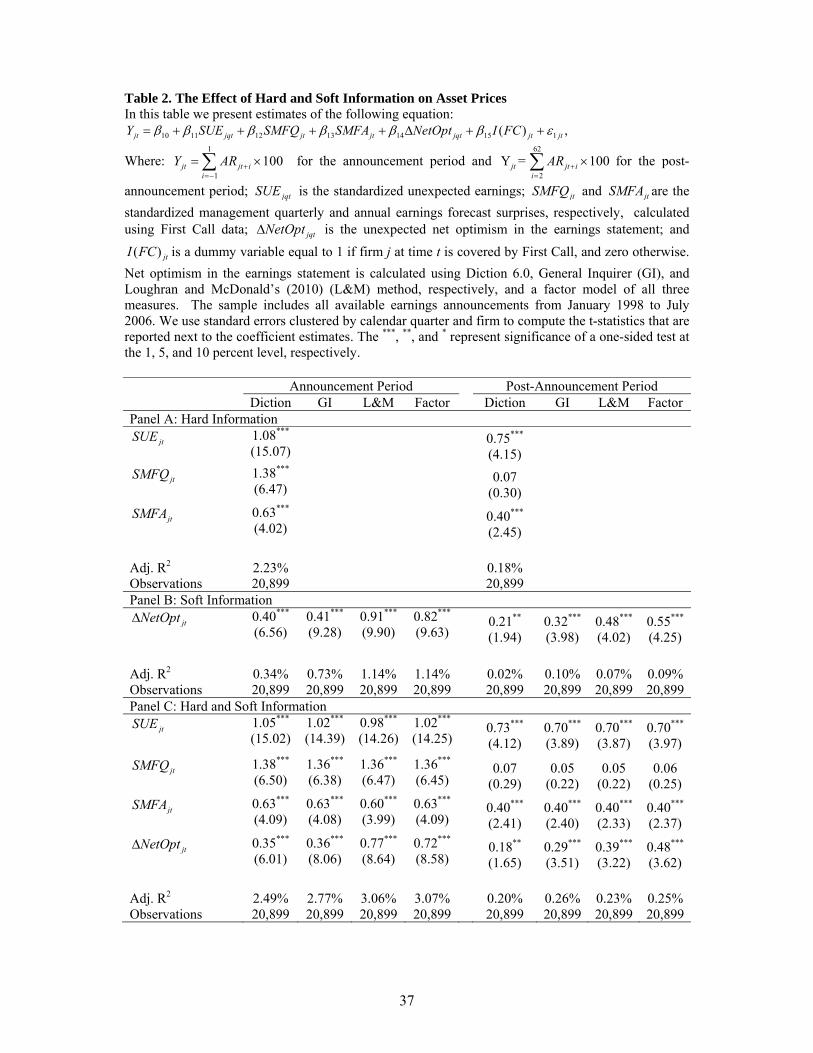
37

Table 2. The Effect of Hard and Soft Information on Asset Prices In this table we present estimates of the following equation:

10 11 12 13 14 15 1( ) ,jt jqt jt jt jqt jt jtY SUE SMFQ SMFA NetOpt I FC

Where: 1

1

100 jt jt ii

Y AR

for the announcement period and 62

2

Y = 100 jt jt ii

AR

for the post-

announcement period; jqtSUE is the standardized unexpected earnings; jtSMFQ and jtSMFA are the

standardized management quarterly and annual earnings forecast surprises, respectively, calculated using First Call data; jqtNetOpt is the unexpected net optimism in the earnings statement; and

( ) jtI FC is a dummy variable equal to 1 if firm j at time t is covered by First Call, and zero otherwise.

Net optimism in the earnings statement is calculated using Diction 6.0, General Inquirer (GI), and Loughran and McDonald’s (2010) (L&M) method, respectively, and a factor model of all three measures. The sample includes all available earnings announcements from January 1998 to July 2006. We use standard errors clustered by calendar quarter and firm to compute the t-statistics that are reported next to the coefficient estimates. The ***, **, and * represent significance of a one-sided test at the 1, 5, and 10 percent level, respectively. Announcement Period Post-Announcement Period Diction GI L&M Factor Diction GI L&M Factor Panel A: Hard Information

jtSUE 1.08*** (15.07)

0.75***

(4.15)

jtSMFQ 1.38*** (6.47)

0.07 (0.30)

jtSMFA 0.63*** (4.02)

0.40*** (2.45)

Adj. R2 2.23% 0.18% Observations 20,899 20,899 Panel B: Soft Information

jtNetOpt 0.40*** (6.56)

0.41*** (9.28)

0.91*** (9.90)

0.82*** (9.63)

0.21** (1.94)

0.32*** (3.98)

0.48*** (4.02)

0.55*** (4.25)

Adj. R2 0.34% 0.73% 1.14% 1.14% 0.02% 0.10% 0.07% 0.09% Observations 20,899 20,899 20,899 20,899 20,899 20,899 20,899 20,899Panel C: Hard and Soft Information

jtSUE 1.05*** (15.02)

1.02*** (14.39)

0.98*** (14.26)

1.02***

(14.25) 0.73***

(4.12) 0.70*** (3.89)

0.70*** (3.87)

0.70*** (3.97)

jtSMFQ 1.38*** (6.50)

1.36*** (6.38)

1.36*** (6.47)

1.36***

(6.45) 0.07

(0.29) 0.05

(0.22) 0.05

(0.22) 0.06

(0.25)

jtSMFA 0.63*** (4.09)

0.63*** (4.08)

0.60*** (3.99)

0.63*** (4.09)

0.40*** (2.41)

0.40*** (2.40)

0.40*** (2.33)

0.40***

(2.37)

jtNetOpt 0.35*** (6.01)

0.36*** (8.06)

0.77*** (8.64)

0.72*** (8.58)

0.18** (1.65)

0.29***

(3.51) 0.39*** (3.22)

0.48*** (3.62)

Adj. R2 2.49% 2.77% 3.06% 3.07% 0.20% 0.26% 0.23% 0.25% Observations 20,899 20,899 20,899 20,899 20,899 20,899 20,899 20,899

38

Table 3. The Effect of Soft Information on the Post-Announcement Drift In Panel A, each calendar quarter stocks are classified in one of three groups according to their earnings announcement surprise terciles. The surprise tercile for firm j in quarter q is a ranking from 1 to 3 of the earnings surprise, SUEjqt , based on the previous quarter’s surprise tercile cutoffs. In Panel B, each calendar quarter stocks are classified in one of three groups according to their earnings announcement surprise terciles and net optimism surprise terciles. The surprise tercile for firm j in quarter q is a ranking from 1 to 3 of the earnings surprise, SUEjqt , and net optimism surprise, ∆NetOptjqt, based on the previous quarter’s surprise tercile cutoffs. NetOptjqt is calculated using a factor model of the net optimism measures we obtain using the Diction 6.0 software, General Inquirer and Loughran and McDonald’s (2010) method. For Panel B, a firm is included in tercile 1 if both surprises fall into the first tercile, in tercile 2 if both surprises fall into the second tercile, and in tercile 3 if both surprises fall into the third tercile. The 3-day CAR is the cumulative size- and B/M-adjusted return over trading days [-1,+1], where day 0 is the earnings announcement date. The 60-day CAR is the cumulative size- and B/M-adjusted return over trading days [+2, +62]. The cumulative returns are multiplied by 100. Firms in market capitalization deciles 9 and 10 are assigned to the large-firm group, firms in deciles 6 through 8 are assigned to the medium-firm group and those in deciles 1 to 5 are assigned to the small-firm group. Three, two and one asterisk denote, respectively, that the estimates are statistically significant at the one, five and ten percent level.

Panel A: Sorting on SUE

Tercile SUE 3-Day CAR 60-Day CAR 3-1

Small

1 -0.961*** -2.024*** -2.042***

2 0.065*** -0.126*** -0.561**

3 1.083*** 2.959*** 1.238*** 3.280*** Medium

1 -0.984*** -0.560*** 0.304

2 0.075*** 0.283* 0.920***

3 1.073*** 1.454*** 1.826*** 1.522*** Large

1 -0.934*** -0.179 -0.635

2 0.081*** 0.393** 0.018

3 0.980*** 1.097*** 0.433 1.068

Panel B: Sorting First on SUE and then on ∆NetOpt

Tercile SUE ∆NetOpt 3-Day CAR 60-Day CAR 3-1

Small

1 -1.028*** -1.172*** -3.111*** -3.103***

2 0.065*** -0.024*** -0.097 -0.191

3 1.087*** 1.040*** 4.570*** 2.362*** 5.465***

Medium

1 -1.057*** -1.012*** -1.317*** 0.467

2 0.075*** -0.029*** 0.242 0.628

3 1.075*** 0.971*** 2.242*** 2.890*** 2.424**

Large

1 -1.021*** -1.053*** -0.462 -1.298

2 0.084*** -0.037*** 0.413* -0.163

3 0.965*** 0.922*** 1.474*** 0.034 1.331

39

Table 4. Net Optimism as a Complement to Hard Information In this table we present estimates of the following equation:

1

21 22 23 241 1 1 1 1

25 26 27 28

100

Z Z Z Z

jt i z jqt zjt z jt zjt z jt zjt z jqt zjti z z z z

jqt jt jt jt jt jt jqt jt

AR SUE X SMFQ X SMFA X NetOpt X

SUE Size SMFQ Size SMFA Size NetOpt Size

29 210 211 21

( ) ,Z

z zjt jt jt jtz

X I FC Size

Where: jqtSUE is the standardized unexpected earnings; jtSMFQ and jtSMFA are the standardized

management quarterly and annual earnings forecast surprises, respectively, calculated using First Call data; jqtNetOpt is the unexpected net optimism in the earnings statement calculated using a factor

model of the measures we obtain using the Diction 6.0 software, General Inquirer and Loughran and McDonald’s (2010) method; ( ) jtI FC is a dummy variable set equal to 1 if firm j at time t is covered

by First Call, and zero otherwise; jtSize is the log market capital of firm j at time t; and zjtX are

dummy variable proxies for the information environment. The proxies include a dummy variable set equal to one if the firm is in the high tech sector, a dummy variable set equal to one if the firm invests in research and development, and three dummy variables set equal to 1 if the EFKOS e-loadings or PE ratios of firm j at time t respectively belong to the bottom, middle, or top third of each variable’s distribution. The sample includes all available earnings announcements from January 1998 to July 2006. We use standard errors clustered by calendar quarter and firm to compute the χ2-statistics that are reported in parenthesis below the total effect estimates, which are calculated as

. .z zjt jtX Size . The ***, **, and * represent the significance of a one-sided test at the 1, 5, and

10 percent level, respectively.

High Tech R&D Expenses EFKOS e-Loading PE Ratio

jt jtSUE X

Low 1.00***

(239.58) 0.93***

(147.52) 0.84*** (67.31)

1.13*** (77.03)

Medium NA

NA

0.85*** (60.24)

0.72*** (86.36)

High 0.99***

(40.64) 1.24*** (55.52)

1.30*** (74.26)

0.97***

(48.95)

Low-High 0.01 (0.00)

-0.31** (3.15)

-0.45*** (6.38)

0.16 (1.30)

jt jtNetOpt X

Low 0.60*** (68.23)

0.66*** (48.64)

0.50*** (8.97)

0.84*** (52.79)

Medium NA NA 0.64*** (38.03)

0.48*** (19.47)

High 0.92***

(42.19) 0.99*** (26.41)

0.80*** (32.44)

0.45*** (8.82)

Low-High -0.32** (4.24)

-0.33** (2.68)

-0.30*

(2.28)-0.39** (4.94)

Adj. R2 3.55% 2.81% 3.52% 3.62% Observations 20,899 20,899 20,688 17,135

40

Table 5. Credibility of Net Optimism In this table we present estimates of the following equation:

1 3 3 3 3

31 32 33 341 1 1 1 1

35 36 37 38

100

jt i z jqt zjt z jt zjt z jt zjt z jqt zjti z z z z

jqt jt jt jt jt jt jqt jt

AR SUE X SMFQ X SMFA X NetOpt X

SUE Size SMFQ Size SMFA Size NetOpt Size

3

39 310 311 31

( ) ,z zjt jt jt jtz

X I FC Size

Where: jqtSUE is the standardized unexpected earnings; jtSMFQ and jtSMFA

are the standardized

management quarterly and annual earnings forecast surprises, respectively, calculated using First Call data; jqtNetOpt is the unexpected net optimism in the earnings statement calculated using a factor

model of the measures we obtain using the Diction 6.0 software, General Inquirer and Loughran and McDonald’s (2010) method; ( ) jtI FC is a dummy variable set equal to 1 if firm j at time t is covered

by First Call, and zero otherwise; jtSize is the log of the market capitalization of firm j at time t; and

1 2 3, and jt jt jtX X X

are dummy variables equal to 1 if the exogenous variable (media coverage,

turnover, numerical terms in the earnings statement, or the Hutton-Stocken measure of manager’s reputation) of firm j at time t belongs to the bottom, middle, ortop third of each variable’s respective distribution. The sample includes all available earnings announcements from January 1998 to July 2006. We use standard errors clustered by calendar quarter and firm to compute the χ2-statistics that are reported next to the total effect estimates, which are calculated as . .z zjt jtX Size . The ***, **, and * represent the significance of a one-sided test at the 1, 5, and 10 percent level, respectively.

Numerical Terms

Analyst Coverage

Media Coverage

Turnover Manager’s Reputation

jt jtSUE X

Low 1.16*** (108.31)

1.11***

(164.91) 0.81***

(45.22) 0.85***

(100.15)

0.34**

(3.73)

Medium 1.03***

(62.51) 0.66***

(19.68) 1.01***

(42.54) 0.96***

(91.82)

0.82***

(21.38)

High 0.72***

(49.77) 0.97***

(47.59) 1.24***

(85.04) 1.21***

(54.29)

0.75***

(18.06)

Low-High 0.44***

(12.66) 0.14

(0.92) -0.43***

(5.21) -0.37**

(3.63)

-0.41**

(2.58)

jt jtNetOpt X

Low 0.58***

(20.29) 0.48***

(21.26) 0.57***

(28.98) 0.20***

(29.98)

0.50***

(7.42)

Medium 0.63***

(34.69) 0.74***

(18.69) 0.52***

(16.22) 0.27***

(17.56)

0.35**

(3.37)

High 0.82***

(23.40) 1.03 ***

(30.91) 0.93***

(20.55) 0.57***

(20.46)

0.93***

(22.55)

Low-High -0.24*

(1.80)-0.35***

(6.84)-0.37*

(2.38)-0.37**

(3.34)

-0.43**

(2.55) Adj. R2 3.58% 3.60% 3.59% 3.64% 3.50% Observations 20,899 20,899 20,899 20,899 6,284

41

Table 6. Complementarity and Credibility of Soft Information In this table we present estimates of the following equation:

1 4 4

40 41 42 43 431 1 1

4 4

44 44 45 451 1

100

jt i jqt k jqt kjt jt k jt kjti k k

jt k jt kjt jqt k jqt kjtk k

AR SUE SUE X SMFQ SMFQ X

SMFA SMFA X NetOpt NetOpt X

4

46 47 41

( ) ,k kjt jt jtk

X I FC

Where: jqtSUE is the standardized unexpected earnings; jtSMFQ and jtSMFA are the standardized

management quarterly and annual earnings forecast surprises, respectively, calculated using First Call data; jqtNetOpt is the unexpected net optimism in the earnings statement calculated using a factor

model of the measures we obtain using the Diction 6.0 software, General Inquirer and Loughran and McDonald’s (2010) method; ( ) jtI FC

is a dummy variable set equal to 1 if firm j at time t is covered

by First Call, and zero otherwise; 1 jtX is the log of the market capitalization of firm j at time t; 2 jtX

is the EFKOS e-loading of firm j at time t; 3 jtX is the proportion of numerical terms to the total

number of words contained in the earnings statement of firm j at time t; and 4 jtX is the turnover of

firm j at time t. The sample includes all available earnings announcements from January 1998 to July 2006. We use standard errors clustered by calendar quarter and firm to compute the t-statistics that are reported in parenthesis below the coefficient estimates. The ***, **, and * represent significance of one-sided tests at the 1, 5, and 10 percent level, respectively.

jtSUE 6.44***

(7.87)

jt jtSUE Size -0.25***

(-6.18) EFKOS e loadingjt jtSUE 0.43**

(1.84) Numerical Termsjt jtSUE -0.03***

(-2.85)

jt jtSUE Turnover -0.02 (-0.30)

jtNetOpt 3.32***

(2.95)

jt jtNetOpt Size -0.15***

(-2.96) EFKOS e loadingjt jtNetOpt 0.66***

(2.76)Numerical Termsjt jtNetOpt 0.02**

(2.28)

jt jtNetOpt Turnover 0.07**

(1.97) Adj. R-squared 3.85% Observations 20,688

42

Table 7. Correlation Matrix of the Level of Certainty in the Earnings Statement and Measures of Uncertainty In this table we present in Panel A the pairwise spearman correlations between the level of certainty in the earnings statement and various measures of uncertainty used in the previous literature. We present in Panel B the results of a multivariate regression of certainty on the various measures of uncertainty. Certainty in the earnings statement is measured using the Diction 6.0 software and the Loughran and McDonald’s (2010) (L&M) method, respectively, and a factor model of the two measures. The ***, **, and * represent significance of one-sided tests at the 1, 5, and 10 percent level, respectively. Diction L&M Factor

Panel A: Pairwise Correlation with Certainty Earnings Volatility -0.122*** -0.052*** -0.110***

R2 of Seasonal RW Model for EPS 0.053*** 0.050*** 0.067***

Inv. of manager’s forecast precision -0.084*** -0.042*** -0.080***

Dispersion across analysts’ forecasts -0.103*** -0.056*** -0.010***

Turnover -0.141*** -0.137*** -0.173***

PE Ratio -0.084*** -0.068*** -0.097***

R&D Expenditures -0.240*** -0.066*** -0.195***

High Tech -0.151*** -0.034*** -0.119***

Panel B: Multiple Regression Analysis

Earnings Volatility -0.043** -0.003 -0.0004 -0.001 -0.004* -0.002

(-1.92) (-0.10) (-0.46) (-0.68) (-1.61) (-0.53)

R2 of Seasonal RW Model for EPS 2.961*** 2.429** 0.066* -0.027 0.307*** 0.128

(3.07) (2.19) (1.39) (-0.43) (2.87) (1.00)

Dispersion across analysts’ forecasts NA -1.649*** NA -0.022 NA -0.149***

(-2.72) (-0.94) (-2.73)

Turnover -0.322*** -0.447*** -0.011** -0.022** -0.039*** -0.065***

(-3.43) (-2.51) (-1.76) (-2.01) (-2.74) (-2.40)

PE Ratio -0.005*** -0.004*** -0.00004 0.00005* -0.0004*** -0.0002**

(-6.69) (-4.52) (-1.09) (1.41) (-5.25) (-2.06)

R&D Expenditures -13.300*** -10.988*** -0.149 -0.160 -1.155*** -1.008***

(-5.52) (-3.02) (-1.19) (-0.87) (-4.22) (-2.36)

High Tech -1.884*** -1.563*** -0.041** -0.046* -0.193*** -0.180***

(-4.77) (-3.02) (-1.79) (-1.56) (-4.40) (-2.87)

Linear Time Trend -0.004*** -0.003*** -0.0001*** -0.0001*** -0.001*** -0.0004***

(-4.28) (-3.12) (-4.56) (-2.98) (-5.04) (-3.49)

Adjusted R-squared 4.09% 3.21% 1.39% 1.27% 4.35% 3.51%

Observations 20,899 13,349 20,899 13,349 20,899 13,349

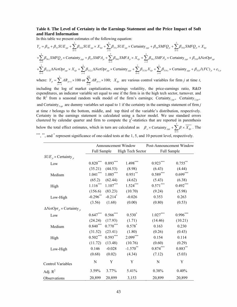
43

Table 8. The Level of Certainty in the Earnings Statement and the Price Impact of Soft and Hard Information In this table we present estimates of the following equation:

7 3 7

50 51 52 53 54 551 1 1

3 7 3

56 57 58 59 5101 1 1

Certainty

Certainty Certainty

jt jqt k jqt kjt z jqt zjqt jt k jt kjtk z k

z jt zjqt jt k jt kjt z jt zjqtz k z

Y SUE SUE X SUE SMFQ SMFQ X

SMFQ SMFA SMFA X SMFA NetO

7 3 7 3

511 512 513 514 515 51 1 1 1

Certainty Certainty ( )

jqt

k jqt kjt z jqt zjqt k kjt z zjqt jt jtk z k z

pt

NetOpt X NetOpt X I FC

where: 1 62

1 2

100 or 100; jt jt i jt ii i

Y AR AR

kjtX are various control variables for firm j at time t,

including the log of market capitalization, earnings volatility, the price-earnings ratio, R&D expenditures,

an indicator variable set equal to one if the firm is in the high tech sector, turnover, and

the R2 from a seasonal random walk model of the firm’s earnings; 1Certainty ,jqt 2Certainty ,jqt

3and Certainty jqt are dummy variables set equal to 1 if the certainty in the earnings statement of firm j

at time t belongs to the bottom, middle, and top third of the variable’s distribution, respectively. Certainty in the earnings statement is calculated using a factor model. We use standard errors clustered by calendar quarter and firm to compute the χ2-statistics that are reported in parenthesis

below the total effect estimates, which in turn are calculated as 7

. .1

Certaintyz zjqt kjtk

X

. The

***, **, and * represent significance of one-sided tests at the 1, 5, and 10 percent level, respectively.

  Announcement Window Post-Announcement Window

  Full Sample High Tech Sector Full Sample

Certaintyjt jtSUE

Low 0.820*** 0.893*** 1.498*** 0.923*** 0.755**

(35.21) (44.53) (8.98) (6.43) (4.44)

Medium 1.041*** 1.085*** 0.951** 0.589*** 0.699***

(65.2) (62.44) (4.62) (5.43) (6.38)

High 1.116*** 1.107*** 1.524*** 0.571*** 0.492***

(156.6) (83.23) (10.70) (9.24) (5.98)

Low-High -0.296** -0.214* -0.026 0.353 0.263

(3.56) (1.68) (0.00) (0.80) (0.53)

Certaintyjt jtNetOpt

Low 0.647*** 0.566*** 0.530* 1.027*** 0.996***

(24.24) (17.93) (1.71) (14.46) (10.21)

Medium 0.840*** 0.770*** 0.578* 0.163 0.230

(31.52) (23.41) (1.80) (0.26) (0.43)

High 0.502*** 0.593*** 2.099*** 0.154 0.114

(11.72) (13.48) (10.76) (0.60) (0.29)

Low-High 0.146 -0.028 -1.570** 0.874*** 0.883**

(0.68) (0.02) (4.34) (7.12) (5.03)

Control Variables N Y Y N Y

Adj. R2 3.59% 3.77% 5.41% 0.38% 0.40%

Observations 20,899 20,899 3,153 20,899 20,899

44

Table 9: The Level of Certainty in the Earnings Statement and the Volatility Impact of Net Optimism In this table we present estimates of the following equation:

0 1 1 2 3 4 5 6 7

3

8 9 101

log( ) log( ) ( 0) ( 0) ( 0)

( 0) Certainty

jt jt jqt jqt jqt jqt jqt jqt jt jt jt

jt jt jt z zjqtz

Vol Vol SUE SUE I SUE NetOpt NetOpt I NetOpt SMFQ SMFQ I SMFQ

SMFA SMFA I SMFA

11 12I(FC) jt jtX

where: 1 62 4 62

2 2 2 21

1 2 2 2

or , and or jt jt i jt i jt jt i jt ii i i i

Vol AR AR Vol AR AR

for the announcement and post-announcement period, respectively. We

measure ΔNetOpt and Certainty using the Diction 6.0 software and Loughran and McDonald’s (2010) (L&M) method, respectively, and a factor model that uses both measures. The sample includes all available earnings announcements from January 1998 to July 2006. We use standard errors clustered by calendar quarter and firm to compute the statistical significance. The ***, **, and * represent significance at the 1, 5, and 10 percent level, respectively.

Announcement Period Post-Announcement Period Diction L&M Factor Diction L&M Factor Certainty Low -2.40*** -2.45*** -2.33*** -2.48*** -2.36*** -2.46*** 3.19*** 0.75*** 3.21*** 0.75 3.21*** 0.75*** (196.48) (75.7) (178.68) (78.47) (195.86) (75.24) (664.57) (13.55) (629.01) (14.30) (643.99) (13.92)

Medium -2.60*** -2.54*** -2.42*** -2.48*** -2.47*** -2.48*** 3.10*** 0.72*** 3.17*** 0.74 3.17*** 0.746*** (217.76) (84.63) (207.61) (75.94) (186.1) (79.19) (616.21) (12.63) (619.00) (13.56) (652.72) (13.59)

High -2.73*** -2.54*** -2.50*** -2.50*** -2.65*** -2.51*** 3.03*** 0.72*** 3.17*** 0.73 3.08*** 0.725*** (258.79) (82.46) (207.61) (79.14) (240.7) (79.80) (563.87) (12.43) (625.31) (13.13) (565.46) (12.67)

Low-High 0.33*** 0.09*** -0.15*** 0.02 0.29*** 0.05* 0.16*** 0.03*** 0.04* 0.02 0.13*** 0.02* (137.83) (7.23) (24.12) (0.19) (99.75) (2.30) (26.00) (6.30) (2.23) (0.73) (15.37) (1.68)

Past Volatility 0.32*** 0.22*** 0.32*** 0.21*** 0.32*** 0.21*** 0.29*** 0.52*** 0.30*** 0.51*** 0.29*** 0.51*** (34.34) (19.02) (35.17) (18.95) (34.56) (18.94) (44.98) (28.84) (44.82) (28.78) (44.63) (28.80) Log(Market Cap.) -0.07*** -0.09*** -0.07 -0.10*** -0.07*** -0.094*** -0.23 -0.10*** -0.23*** -0.10*** -0.23*** -0.10*** (-8.16) (-6.86) (-8.62) (-7.03) (-8.51) (-6.91) (-25.82) (-9.27) (-25.66) (-9.30) (-8.51) (-9.21) Other Controls N Y N Y N Y N Y N Y N Y Adjusted R-squared 12.46% 19.11% 11.93% 19.05% 12.32% 19.07% 39.19% 63.0% 38.89% 62.99% 39.08% 62.99%

45

Appendix A First Call Sample Estimates

Table A1. The Effect of Hard and Soft Information on Asset Prices In this table we present estimates of the following equation:

10 11 12 13 14 15 1( ) ,jt jqt jt jt jqt jt jtY SUE SMFQ SMFA NetOpt I FC

Where: 1

1

100 jt jt ii

Y AR

for the announcement period and 62

2

Y = 100 jt jt ii

AR

for the post-

announcement period; jqtSUE is the standardized unexpected earnings; jtSMFQ and jtSMFA are the

standardized management quarterly and annual earnings forecast surprises, respectively, calculated using First Call data; and jqtNetOpt is the unexpected net optimism in the earnings statement. Net

optimism in the earnings statement is calculated using Diction 6.0, General Inquirer (GI), and Loughran and McDonald’s (2010) (L&M) method, respectively, and a factor model of all three measures. The sample includes all available earnings announcements in our First Call sample from January 1998 to July 2006. We use standard errors clustered by calendar quarter and firm to compute the t-statistics that are reported next to the coefficient estimates. The ***, **, and * represent significance of a one-sided test at the 1, 5, and 10 percent level, respectively. Announcement Period Post-Announcement Period Diction GI L&M Factor Diction GI L&M Factor Panel A: Hard Information

jtSUE 1.89*** (17.21)

0.49***

(3.56)

jtSMFQ 1.27*** (6.62)

0.08 (0.34)

jtSMFA 0.51*** (3.47)

0.42*** (2.42)

Adj. R2 7.27% 0.11% Observations 14,649 14,649 Panel B: Soft Information

jtNetOpt 0.33*** (5.31)

0.35*** (8.38)

0.84*** (9.10)

0.69*** (7.37)

0.31*** (2.44)

0.27*** (3.12)

0.55*** (3.42)

0.60*** (3.15)

Adj. R2 0.25% 0.56% 1.03% 0.95% 0.05% 0.08% 0.11% 0.13% Observations 14,649 14,649 14,649 14,649 14,649 14,649 14,649 14,649Panel C: Hard and Soft Information

jtSUE 1.88*** (17.18)

1.86*** (16.75)

1.84*** (16.89)

1.86***

(16.89) 0.48***

(3.41) 0.46*** (3.21)

0.44*** (3.14)

0.45*** (3.20)

jtSMFQ 1.27*** (6.63)

1.25*** (6.54)

1.24*** (6.56)

1.25***

(6.58) 0.08

(0.32) 0.06

(0.26) 0.06

(0.24) 0.06

(0.27)

jtSMFA 0.51*** (3.51)

0.51*** (3.51)

0.49*** (3.44)

0.51*** (3.53)

0.42*** (2.36)

0.42*** (2.40)

0.41** (2.30)

0.42***

(2.36)

jtNetOpt 0.24*** (4.13)

0.25*** (5.91)

0.59*** (6.90)

0.51*** (5.59)

0.29** (2.27)

0.25***

(2.74) 0.50*** (2.94)

0.55*** (3.14)

Adj. R2 7.40% 7.55% 7.78% 7.75% 0.15% 0.17% 0.19% 0.22% Observations 14,649 14,649 14,649 14,649 14,649 14,649 14,649 14,649

46

Table A2. Net Optimism as a Complement to Hard Information In this table we present estimates of the following equation:

1

21 22 23 241 1 1 1 1

25 26 27 28

100

Z Z Z Z

jt i z jqt zjt z jt zjt z jt zjt z jqt zjti z z z z

jqt jt jt jt jt jt jqt jt

AR SUE X SMFQ X SMFA X NetOpt X

SUE Size SMFQ Size SMFA Size NetOpt Size

29 211 21

,Z

z zjt jt jtz

X Size

Where: jqtSUE is the standardized unexpected earnings; jtSMFQ and jtSMFA are the standardized

management quarterly and annual earnings forecast surprises, respectively, calculated using First Call data; jqtNetOpt is the unexpected net optimism in the earnings statement calculated using a factor

model of the measures we obtain using the Diction 6.0 software, General Inquirer and Loughran and McDonald’s (2010) method; jtSize is the log market capital of firm j at time t; and zjtX

are dummy

variable proxies for the information environment. The proxies include a dummy variable set equal to one if the firm is in the high tech sector, a dummy variable set equal to one if the firm invests in research and development, and three dummy variables set equal to 1 if the EFKOS e-loadings or PE ratios of firm j at time t respectively belong to the bottom, middle, or top third of each variable’s distribution. The sample includes all available earnings announcements in our First Call sample from January 1998 to July 2006. We use standard errors clustered by calendar quarter and firm to compute the χ2-statistics that are reported in parenthesis below the total effect estimates, which are calculated as . .z zjt jtX Size . The ***, **, and * represent the significance of a one-sided test at the 1, 5, and

10 percent level, respectively.

High Tech R&D Expenses EFKOS e-Loading PE Ratio

jt jtSUE X

Low 1.72***

(259.74) 1.68***

(178.81) 1.76*** (90.59)

1.73*** (75.02)

Medium NA

NA

1.76*** (169.25)

1.65*** (119.19)

High 2.57***

(72.03) 2.10***

(124.94) 1.99***

(147.94) 2.21***

(142.76) Low-High -0.86***

(9.15) -0.42** (4.16)

-0.23 (1.23)

-0.48** (2.79)

jt jtNetOpt X

Low 0.42*** (27.08)

0.37*** (17.57)

0.18 (1.88)

0.31** (3.48)

Medium NA NA 0.49*** (17.49)

0.44*** (13.14)

High 0.76***

(23.22) 0.96*** (21.17)

0.75*** (27.93)

0.55*** (18.94)

Low-High -0.34** (3.69)

-0.59*** (7.18)

-0.57***

(10.7) -0.24 (1.23)

Adj. R2 8.03% 7.64% 7.60% 8.60% Observations 14,649 14,649 14,649 12,367

47

Table A3. Credibility of Net Optimism In this table we present estimates of the following equation:

1 3 3 3 3

31 32 33 341 1 1 1 1

35 36 37 38

100

jt i z jqt zjt z jt zjt z jt zjt z jqt zjti z z z z

jqt jt jt jt jt jt jqt jt

AR SUE X SMFQ X SMFA X NetOpt X

SUE Size SMFQ Size SMFA Size NetOpt Size

3

39 310 311 31

( ) ,z zjt jt jt jtz

X I FC Size

Where: jqtSUE is the standardized unexpected earnings; jtSMFQ and jtSMFA

are the standardized

management quarterly and annual earnings forecast surprises, respectively, calculated using First Call data; jqtNetOpt is the unexpected net optimism in the earnings statement calculated using a factor

model of the measures we obtain using the Diction 6.0 software, General Inquirer and Loughran and McDonald’s (2010) method; jtSize is the log of the market capitalization of firm j at time t; and

1 2 3, and jt jt jtX X X

are dummy variables equal to 1 if the exogenous variable (media coverage,

turnover, numerical terms in the earnings statement, or the Hutton-Stocken measure of manager’s reputation) of firm j at time t belongs to the bottom, middle, ortop third of each variable’s respective distribution. The sample includes all available earnings announcements in our First Call sample from January 1998 to July 2006. We use standard errors clustered by calendar quarter and firm to compute the χ2-statistics that are reported next to the total effect estimates, which are calculated as

. .z zjt jtX Size . The ***, **, and * represent the significance of a one-sided test at the 1, 5, and 10

percent level, respectively.

Numerical Terms

Analyst Coverage

Media Coverage

Turnover Manager’s Reputation

jt jtSUE X

Low 1.89***

(178.07) 1.60***

(115.26) 1.87***

(99.86) 1.28***

(122.18)

1.69***

(114.81)

Medium 1.80***

(174.12) 2.12***

(127.85) 1.88***

(88.6) 1.91***

(161.07)

1.82***

(158.6)

High 1.78***

(50.83) 1.99***

(94.01) 1.74***

(76.81) 2.24***

(97.52)

2.21***

(179.64)

Low-High 0.10

(0.2) -0.38* (1.92)

0.13(0.23)

-0.97**

(14.93)

-0.51**

(5.00)

jt jtNetOpt X

Low 0.45***

(12.77) 0.31***

(6.53) 0.52***

(23.7) 0.24**

(4.65)

0.29**

(2.48)

Medium 0.53***

(11.45) 0.58***

(9.88) 0.38***

(6.75) 0.46***

(20.96)

0.24

(1.57)

High 0.51***

(18.25) 0.65 ***

(15.39) 0.56***

(14.04) 0.75***

(18.68)

0.94***

(23.38)

Low-High -0.06(0.13)

-0.34*

(2.36)-0.04(0.06)

-0.51***

(5.83)

-0.65***

(5.54) Adj. R2 7.60% 7.80% 7.61% 8.07% 10.09% Observations 14,649 14,649 14,649 14,649 5,757

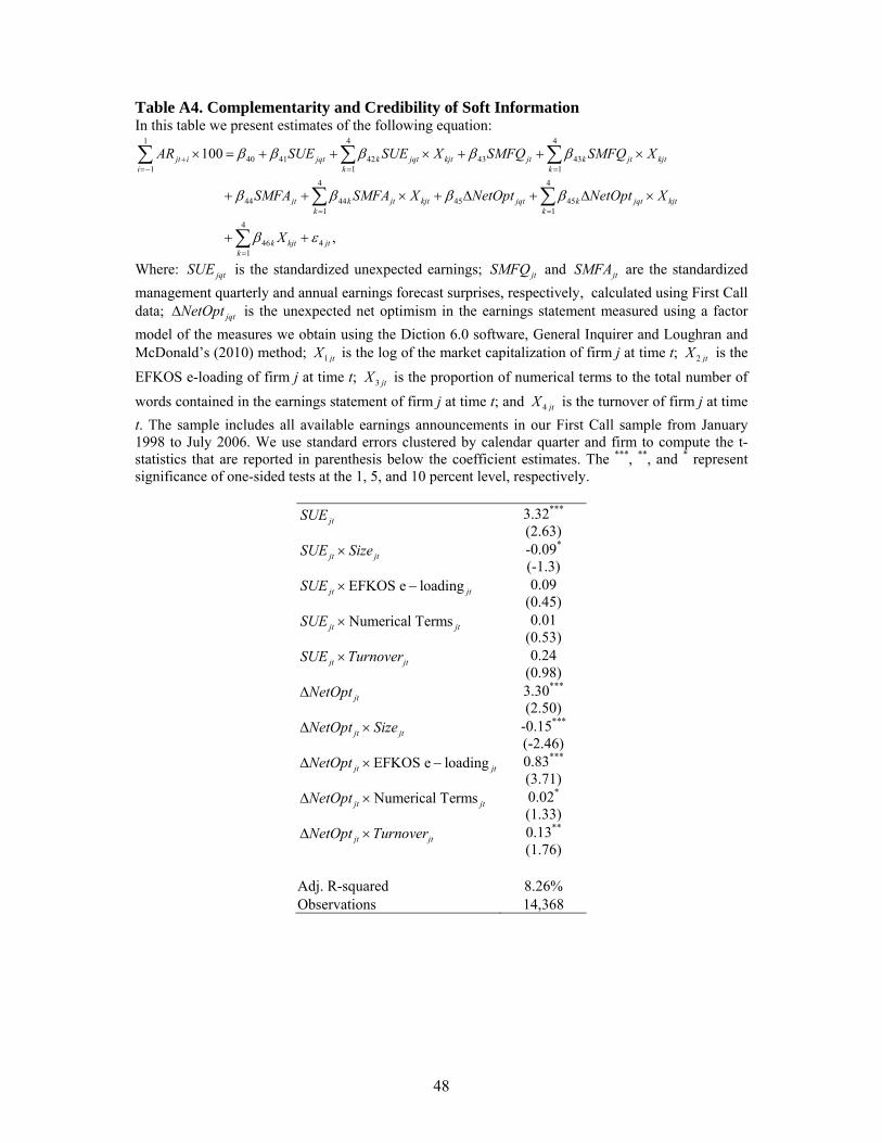
48

Table A4. Complementarity and Credibility of Soft Information In this table we present estimates of the following equation:

1 4 4

40 41 42 43 431 1 1

4 4

44 44 45 451 1

100

jt i jqt k jqt kjt jt k jt kjti k k

jt k jt kjt jqt k jqt kjtk k

AR SUE SUE X SMFQ SMFQ X

SMFA SMFA X NetOpt NetOpt X

4

46 41

,k kjt jtk

X

Where: jqtSUE is the standardized unexpected earnings; jtSMFQ and jtSMFA are the standardized

management quarterly and annual earnings forecast surprises, respectively, calculated using First Call data; jqtNetOpt is the unexpected net optimism in the earnings statement measured using a factor

model of the measures we obtain using the Diction 6.0 software, General Inquirer and Loughran and McDonald’s (2010) method; 1 jtX is the log of the market capitalization of firm j at time t; 2 jtX is the

EFKOS e-loading of firm j at time t; 3 jtX is the proportion of numerical terms to the total number of

words contained in the earnings statement of firm j at time t; and 4 jtX is the turnover of firm j at time

t. The sample includes all available earnings announcements in our First Call sample from January 1998 to July 2006. We use standard errors clustered by calendar quarter and firm to compute the t-statistics that are reported in parenthesis below the coefficient estimates. The ***, **, and * represent significance of one-sided tests at the 1, 5, and 10 percent level, respectively.

jtSUE 3.32***

(2.63)

jt jtSUE Size -0.09*

(-1.3) EFKOS e loadingjt jtSUE 0.09

(0.45) Numerical Termsjt jtSUE 0.01

(0.53)

jt jtSUE Turnover 0.24 (0.98)

jtNetOpt 3.30***

(2.50)

jt jtNetOpt Size -0.15***

(-2.46)EFKOS e loadingjt jtNetOpt 0.83***

(3.71) Numerical Termsjt jtNetOpt 0.02*

(1.33)

jt jtNetOpt Turnover 0.13**

(1.76) Adj. R-squared 8.26% Observations 14,368

49

Table A5. Correlation Matrix of the Level of Certainty in the Earnings Statement and Measures of Uncertainty In this table we present in Panel A the pairwise spearman correlations between the level of certainty in the earnings statement and various measures of uncertainty used in the previous literature. We present in Panel B the results of a multivariate regression of certainty on the various measures of uncertainty. Certainty in the earnings statement is measured using the Diction 6.0 software and the Loughran and McDonald’s (2010) (L&M) method, respectively, and a factor model that uses both measures. The ***, **, and * represent significance of one-sided tests at the 1, 5, and 10 percent level, respectively. Diction L&M Factor

Panel A: Pairwise Correlation with Certainty Earnings Volatility -0.098*** -0.039*** -0.088***

R2 of Seasonal RW Model for EPS 0.053*** 0.048*** 0.056***

Inv. of manager’s forecast precision -0.082*** -0.037*** -0.075***

Dispersion across analysts’ forecasts -0.101*** -0.057*** -0.097***

Turnover -0.126*** -0.110*** -0.152***

PE Ratio -0.089*** -0.052*** -0.093***

R&D Expenditures -0.230*** -0.065*** -0.191***

High Tech -0.146*** -0.038*** -0.121***

Panel B: Multiple Regression Analysis

Earnings Volatility -0.021 -0.006 -0.0005 -0.001 -0.002 -0.001 (-0.75) (-0.19) (-0.44) (-0.65) (-0.77) (-0.56)

R2 of Seasonal RW Model for EPS 2.11** 2.364** 0.026 -0.025 0.191* 0.128

(2.05) (2.11) (0.48) (-0.41) (1.60) (0.96)

Dispersion across analysts’ forecasts NA -1.548*** NA -0.023 NA -0.146***

(-2.45) (-0.98) (-2.48)

Turnover -0.379*** -0.451*** -0.020** -0.022** -0.058*** -0.065***

(-2.95) (-2.50) (-2.24) (-2.02) (-2.88) (-2.39)

PE Ratio -0.005*** -0.004*** 0.00002 -0.00005* -0.0003*** -0.0002**

(-5.58) (-4.77) (0.41) (1.47) (-3.91) (-2.14)

R&D Expenditures -12.64*** -10.41*** -0.155 -0.147 -1.143*** -0.97**

(-4.18) (-2.80) (-0.98) (-0.78) (-3.13) (-2.14)

High Tech -1.72*** -1.62*** -0.045** -0.048* -0.193*** -0.190***

(-3.78) (-3.11) (-1.67) (-1.58) (-3.42) (-2.93)

Linear Time Trend -0.003*** -0.003*** -0.0001*** -0.0001*** -0.0004*** -0.0004***

(-3.57) (-3.23) (-3.49) (-2.85) (-4.05) (-3.49)

Adjusted R-squared 3.46% 3.24% 1.33% 1.20% 3.78% 3.48%

Observations 14,649 13,349 14,649 13,349 14,649 13,349

50

Table A6. The Level of Certainty in the Earnings Statement and the Price Impact of Soft and Hard Information In this table we present estimates of the following equation:

7 3 7

50 51 52 53 54 551 1 1

3 7 3

56 57 58 59 5101 1 1

Certainty

Certainty Certainty

jt jqt k jqt kjt z jqt zjqt jt k jt kjtk z k

z jt zjqt jt k jt kjt z jt zjqtz k z

Y SUE SUE X SUE SMFQ SMFQ X

SMFQ SMFA SMFA X SMFA NetO

7 3 7 3

511 512 513 514 51 1 1 1

Certainty Certainty

jqt

k jqt kjt z jqt zjqt k kjt z zjqt jtk z k z

pt

NetOpt X NetOpt X

where: 1 62

1 2

100 or 100; jt jt i jt ii i

Y AR AR

kjtX are various control variables for firm j at time t,

including the log of market capitalization, earnings volatility, the price-earnings ratio, R&D expenditures,

an indicator variable set equal to one if the firm is in the high tech sector, turnover, and

the R2 from a seasonal random walk model of the firm’s earnings; 1Certainty ,jqt 2Certainty ,jqt

3and Certainty jqt are dummy variables set equal to 1 if the certainty in the earnings statement of firm j

at time t belongs to the bottom, middle, and top third of the variable’s distribution, respectively. Certainty in the earnings statement is calculated using a factor model. We use standard errors clustered by calendar quarter and firm to compute the χ2-statistics that are reported in parenthesis

below the total effect estimates, which in turn are calculated as 7

. .1

Certaintyz zjqt kjtk

X

. The

***, **, and * represent significance of one-sided tests at the 1, 5, and 10 percent level, respectively.

  Announcement Window Post-Announcement Window

  Full Sample High Tech Sector Full Sample

Certaintyjt jtSUE

Low 1.66*** 1.67*** 2.62*** 0.92*** 0.74***

(110.35) (110.55) (53.26) (15.42) (8.03)

Medium 1.84*** 1.82*** 2.45*** 0.38** 0.94**

(184.09) (170.6) (24.46) (3.65) (3.17)

High 1.96*** 1.88*** 2.20*** 0.13 0.12

(136.54) (146.05) (47.59) (0.23) (0.25)

Low-High -0.30** -0.21 0.42 0.79*** 0.62***

(2.77) (1.43) (0.75) (5.05) (3.29)

Certaintyjt jtNetOpt

Low 0.49*** 0.43*** 0.45 0.98*** 1.01 ***

(9.41) (7.83) (1.07) (11.23) (11.18)

Medium 0.74*** 0.66*** 0.73** 0.44 0.42

(20.8) (18) (2.94) (1.56) (1.17)

High 0.25*** 0.32*** 1.28*** 0.17 0.15

(4.18) (7.01) (7.54) (0.47) (0.25)

Low-High 0.24 0.11 -0.82* 0.81** 0.87**

(1.28) (0.34) (2.42) (4.03) (3.24)

Control Variables N Y Y N N

Adj. R2 7.70% 8.24% 12.36% 0.31% 0.45%

Observations 14,649 14,649 2,211 14,649 14,649

51

Table A7: The Level of Certainty in the Earnings Statement and the Volatility Impact of Net Optimism In this table we present estimates of the following equation:

0 1 1 2 3 4 5 6 7

3

8 9 101

log( ) log( ) ( 0) ( 0) ( 0)

( 0) Certainty

jt jt jqt jqt jqt jqt jqt jqt jt jt jt

jt jt jt z zjqtz

Vol Vol SUE SUE I SUE NetOpt NetOpt I NetOpt SMFQ SMFQ I SMFQ

SMFA SMFA I SMFA

12 jtX

where: 1 62 4 62

2 2 2 21

1 2 2 2

or , and or jt jt i jt i jt jt i jt ii i i i

Vol AR AR Vol AR AR

for the announcement and post-announcement period, respectively. We

measure ΔNetOpt and Certainty using the Diction 6.0 software and Loughran and McDonald’s (2010) (L&M) method, respectively, and a factor model that uses both measures. The sample includes all available earnings announcements in our First Call sample from January 1998 to July 2006. We use standard errors clustered by calendar quarter and firm to compute the statistical significance. The ***, **, and * represent significance at the 1, 5, and 10 percent level, respectively.

Announcement Period Post-Announcement Period Certainty Diction L&M Factor Diction L&M Factor Low -2.42*** -2.82*** -2.36*** -2.88*** -2.40*** -2.86*** 2.59*** 0.82*** 2.62*** 0.81*** 2.60*** 0.81*** (120.00) (67.15) (106.83) (71.16) (115.39) (66.40) (183.64) (22.18) (179.23) (22.99) (177.37) (21.87) Medium -2.61*** -2.90*** -2.42*** -2.85*** -2.50*** -2.85*** 2.50*** 0.76*** 2.58*** 0.84*** 2.56*** 0.82*** (142.75) (73.85) (113.44) (69.02) (132.36) (68.93) (171.94) (18.07) (170.79) (23.94) (178.09) (22.44) High -2.68*** -2.88*** -2.45*** -2.86*** -2.63*** -2.87*** 2.46*** 0.77*** 2.60*** 0.79*** 2.51*** 0.77*** (151.37) (73.76) (122.44) (70.31) (147.68) (71.60) (162.17) (17.68) (176.81) (19.93) (157.16) (17.93) Low-High 0.26*** 0.06** 0.08** -0.02 0.22*** 0.01 0.13*** 0.06*** 0.01 0.02 0.09** 0.04** (48.11) (2.87) (4.58) (0.29) (24.75) (0.14) (10.38) (10.16) (0.09) (0.68) (3.85) (2.83) Past Volatility 0.26*** 0.19*** 0.27*** 0.20*** 0.27*** 0.20*** 0.26*** 0.47*** 0.26*** 0.47*** 0.26*** 0.47*** (22.22) (16.22) (21.88) (16.13) (22.18) (16.1) (33.02) (25.09) (33.22) (24.91) (33.29) (24.82) Log(Market Cap.) -0.09*** -0.08*** -0.09 -0.08*** -0.09*** -0.085*** -0.21 -0.11*** -0.21*** -0.11*** -0.21*** -0.11*** (-11.95) (-4.85) (-8.58) (-4.90) (-8.45) (-4.93) (-13.11) (-11.41) (-17.75) (-11.70) (-17.79) (-11.35) Other Controls N Y N Y N Y N Y N Y N Y Adjusted R-squared 8.74% 16.51% 8.35% 16.47% 8.61% 16.47% 32.11% 54.89% 31.87% 54.85% 31.98% 54.86%

52

Appendix B

Evaluating Different Measures of Unanticipated Net-Optimism

Economic theory predicts that only new information should affect asset prices, and

hence our announcement period pricing equation (1) models event period abnormal returns as

a function of unanticipated hard information and of unanticipated net optimism. Our

measures of unanticipated hard information in the Compustat and First Call samples are

standard in the literature whereas our measure of unanticipated net optimism is novel.38 In

this appendix we consider different measures of unanticipated net optimism and conclude

that, among the models that we consider, the best predictor of net optimism for the current

quarter is the prior quarter’s net optimism.

Time Series Models

Based on the earnings forecast literature and because our time series of sentiment is

not very long, we consider a small set of very parsimonious models; at most we estimate only

two parameters.39 The models that we consider are the following:

10 11 1 ' 1 ,jqt j j jq t jtNetOpt NetOpt (A1)

1 ' 2 ,jqt jq t jtNetOpt NetOpt (A2)

30 31 4 ' 3 ,jqt j j jq t jtNetOpt NetOpt (A3)

4 ' 4 ,jqt jq t jtNetOpt NetOpt (A4)

where jqtNetOpt is equal to the number of positive words minus the number of negative

words in firm j’s earnings press release for fiscal quarter q released on day t, divided by the

total number of words in the press release, calculated using a factor model of the sentiment

measures we obtain from Diction 6.0, General Inquirer (GI), and the Loughran and

McDonald (2010) algorithms. The first model (A1) is an autoregressive model of order one

(i.e., an AR(1) model). In the second model (A2) we constrain the constant in equation (A1)

38 To the best of our knowledge Davis et al. (2008) is the only other study to consider unanticipated net optimism. Although their primary analyses implicitly treat all net optimism as unanticipated, in a specification check they consider optimism to follow a random walk. They do not, however, provide an extensive analysis of their measure. 39 Our sample starts in January 1998 and ends in July 2006. The theoretical maximum number of time series observations for a firm in our sample is thus only 34, which is a small number of data points for evaluating the out-of-sample forecasting performance of time series models. Empirically, due to the difficulties of matching uncoded text files into the CRSP/Compustat database, combined with the possibility that firms may choose to file their earnings announcements with other newswire services, we do not have a full set of 34 consecutive observations available for most of the firms in our sample.

53

to be equal to zero and the slope coefficient to be equal to one ( 10 110 and 1j j ). In

other words, in (A2) we assume that net optimism follows a random walk, and thus that the

best predictor of net optimism this quarter is last quarter’s net optimism. The residual of

equation (A2) is Davis et al. (2007)’s measure of unexpected net optimism. The third model

(A3) is a seasonally-adjusted time series model. In the fourth model (A4) we constrain the

constant in equation (A3) to be equal to zero and the slope coefficient to be equal to one

( 30 310 and 1j j ), so that the best predictor of net optimism this quarter is last year’s

same quarter net optimism. This is the standard model of expected earnings per share and the

model that we use to calculate the Compustat sample’s SUE. The advantage of models (A2)

and (A4) over models (A1) and (A3) is that we do not need to estimate any coefficients.

Given the short time-series underlying our sample, this is an important advantage.

To evaluate these four models we follow two different strategies. First, we use our

full sample of firms (5,023 unique CRSP identifiers), constrain the constant and slope

coefficient to be the same across firms, and estimate each model (A1-A4) on the pooled data.

Second, we constrain the sample to firms for which we have a long enough time series to

estimate models (A1-A4) separately for each firm, which means that we only use firms with

at least 4 years of consecutive PR Newswire earnings statement press releases (155 unique

CRSP identifiers).

In Table A8 Panel A, we report the pooled estimation results. We report in-sample

and out-of-sample period root mean squared errors (RMSE) for all four models, as well as the

in-sample R-squared for models (A1) and (A3). We estimate each model by pooling the in-

sample data from January 1998 to June 2005, and then we use the estimated coefficients to

forecast net optimism one quarter ahead for each of the following four quarters (i.e., from

July 2005 to July 2006). In each out-of-sample forecast round we expand the in-sample

period to include the latest quarter, however we only report the in-sample R-squared and

RMSE for the original in-sample period (i.e., from January 1998 to June 2005). The

interesting comparison of in-sample performance is between models (A1) and (A3), because

by definition the in-sample RMSE for models (A1) and (A3) are smaller than those for (A2)

and (A4), respectively. In-sample, model (A1) fits net optimism better than model (A3).

Even though the difference in RMSE for net optimism appears to be small (0.8 compared to

0.9 is an 11% decrease in RMSE), the difference is statistically significantly different from

zero at the 1% level and the difference in R-squares between the two models, 10% versus

almost 30%, is large. We therefore conclude that an AR(1) model fits the data better in-

54

sample than the seasonal time-series model. This finding is consistent with anecdotal

observations that the press releases tend to contain a comparison of this quarter’s earnings

performance to last year’s same quarter performance, and hence the raw net optimism is

already implicitly relative to last year’s same quarter status. The finding that the soft

information consists of an implicit update to the prior benchmark is in contrast to the bottom

line earnings per share model selection for which our results are consistent with prior studies;

the seasonally-adjusted time-series model outperforms the AR(1) model.

Comparing the out-of-sample RMSE of models (A1) and (A3) in the pooled

estimation, which is our preferred criteria for choosing the best model, we reach the same

conclusion because the out-of-sample performance of model (A1) is better than that of (A3).

In fact, model (A1) has the smallest out-of-sample RMSE out of all of the models that we

consider.

In Table A8 Panel B, we report the average (across firms) in-sample and out-of-

sample period RMSE when we estimate models (A1-A4) separately for each firm, as well as

the average R-squared for models (A1) and (A3). We define the in-sample period for firm j

as the full sample for firm j minus the last four quarters. We use the estimated in-sample

coefficients for each firm to forecast net optimism one quarter ahead for each of the last four

quarters in the time series. The results from this estimation indicate that the in-sample

performance of the AR(1) model is slightly better than the seasonally-adjusted time-series

model performance, although the difference in performance is not statistically nor

economically significant. Importantly, in contrast to the pooled estimation, we find that the

firm-specific random walk model (A2) has the smallest out-of-sample RMSE out of all of the

models that we consider. This is perhaps not surprising because when we estimate each

model separately for each firm we do not have enough observations to consistently estimate

the parameters in-sample and thus according to the principle of parsimony the out-of-sample

forecasting performance of (A1) may be worse than that of (A2), and indeed we find that this

is the case.

The pooled estimation and the firm-by-firm estimation both favor an AR(1) model

over the seasonally-adjusted time-series model (i.e., (A1) over (A3)). However, the pooled

estimation favors the (A1) model over the (A2) model, while the firm-by-firm estimation

favors the (A2) model over the (A1) model. As we mentioned above, the advantage of model

(A2) over model (A1) is that we do not need to estimate any coefficients. Given our short

time-series of data, this is an important advantage. Furthermore, we reject the null hypothesis

that the constant and slope coefficients in models (A1) and (A3) are the same across firms, so

55

that our firm-by-firm estimation is better specified than the pooled estimation. Finally, when

estimating unexpected net optimism using (A2), our regression results do not suffer from a

hindsight bias. Taking these three facts into consideration, we define unexpected net

optimism as the difference NetOptjqt=NetOptjqt-NetOptjq-1t’, which is the residual of the (A2)

model. This is the measure of unexpected net optimism used by Davis et al (2007), and also

the best out-of-sample performing model when we estimate each model separately for each

firm.

Robustness Checks

In this section, we gauge the robustness of our results. First, we assess the sensitivity

of our results to six different definitions of unanticipated net optimism. Second, we explore

the possibility that our sentiment variable may simply reflect the characteristics of the CFO.

Robustness to different definitions of unanticipated net optimism

In Table A9 we show coefficient estimates for the announcement period pricing

equation (1) using different definitions of unexpected sentiment. We consider six different

definitions of unanticipated net optimism: the residual of each of models (A1-A4),

respectively, all estimated using the pooled sample, to maximize the sample size; raw net

optimism; and de-meaned net optimism. The number of observations in Table A9 is different

from the total number of observations in our full sample because we further constrain the

sample to firms that have at least four consecutive quarters of sentiment data so that we hold

the sample constant while comparing across models.

Table A9 contains a number of noteworthy findings. First, raw sentiment affects asset

prices. This finding is consistent with the observation that the press releases tend to contain a

comparison of the firm’s earnings performance with the same quarter last year’s

performance, and hence the raw net optimism expressed is already implicitly relative to an

expectational benchmark. The second observation is that the market’s response to raw

sentiment is nevertheless weaker than its response to the “surprise” sentiment, suggesting that

the market realizes that net optimism is serially correlated. Third, the differences in adjusted

R-squares across specifications are very small, and hence the misspecification error is also

small. Fourth, the de-meaned sentiment affects asset prices, so that our sentiment variable

does not simply reflect a CFO characteristic. We further investigate this issue below.

56

Firm Fixed Effects

In this section we consider the possibility that our sentiment variable simply reflects

the characteristics of the CFO. In other words we are concerned that our sentiment variable

is of the form:

2, ~ (0, ),jqt j jqt jqt jNetOpt WN (A5)

and thus we would obtain similar results if we simply replaced the sentiment variable by a

firm fixed effect in our baseline announcement period pricing equation (1). In our pricing

equation, abnormal returns are a function of unexpected net optimism, jqtNetOpt , so that if

raw net optimism is of the form (A5) then jqt jqtNetOpt does not contain a firm fixed

effect. Nevertheless, our unexpected sentiment variable could be of the form:

2, ~ (0, ).jqt j jqt jqt jNetOpt WN (A6)

This is unlikely to be the case, however, given that we cannot reject the null hypothesis that

the time series mean of jqtNetOpt is equal to zero for 99% of our firms. Nevertheless, we

evaluate these two possibilities by estimating a firm fixed effect regression. In particular we

estimate the following two equations:

1

1 11 12 11

,jt i j jqt jqt jti

AR SUE NetOpt

(A7)

1

2 21 22 21

,jt i j jqt jqt jti

AR SUE NetOpt

(A8)

where jqtSUE is the standardized unexpected earnings, jqtNetOpt is raw net optimism in the

earnings statement, and 1 'jqt jqt jq tNetOpt NetOpt NetOpt , is the unexpected net optimism

in the earnings statement. We report the estimation results of (A7) and (A8) with and without

fixed effects (i.e., we set 1 20 and 0 j j j ) in Table A10. The results indicate that

some of the explanatory power of sentiment comes from the within firm sentiment variation

and some of the explanatory power comes from between firm variation. Most importantly,

sentiment is statistically significant even after including a firm fixed effect in our

specification. Our baseline pricing equation will not contain a firm fixed effect because our

hypothesis tests rely on the heterogeneity across firms.

57

Table A8. Unexpected Sentiment

In Panel A, we report the pooled estimation results. We report in-sample and out-of-sample period root mean squared errors (RMSE) for models A1-A4, as well as the in-sample R-squared for models A1 and A3. We estimate each model using pooled data from January 1998 to June 2005, and we use the estimated coefficients to forecast net optimism one quarter ahead for four quarters (from July 2005 to July 2006). In each out-of-sample forecast round we expand the in-sample period to include the latest quarter; however we only report the in-sample R-squared and RMSE for the period January 1998 to June 2005. In Panel B, we report the average (across firms) in-sample and out-of-sample period RMSE when we estimate models A1-A4 separately for each firm, as well as the average R-squared for models A1 and A3. We define the in-sample period for firm j as the full sample for firm j minus the last four quarters. We define net optimism as the first factor of net optimism extracted from three different sources: Diction 6.0 software, General Inquirer (GI), and Loughran and McDonald’s (2010) (L&M) method.

Panel A: Pooled Data Panel B: Time Series

Model A1: 10 11 1 ' 1jqt j j jq t jtNetOpt NetOpt

In-sample RMSE 0.800 0.592 In-sample R-squared 29.69% 13.56% Out-of-sample RMSE 0.738 0.628

Model A2: 1 ' 2jqt jq t jtNetOpt NetOpt

In-sample RMSE 0.924 0.826 Out-of-sample RMSE 0.818 0.603

Model A3: 30 31 4 ' 3jqt j j jq t jtNetOpt NetOpt

In-sample RMSE 0.904 0.594 In-sample R-squared 10.30% 13.48% Out-of-sample RMSE 0.832 0.707

Model A4: 4 ' 4jqt jq t jtNetOpt NetOpt

In-sample RMSE 1.131 1.016 Out-of-sample RMSE 0.969 0.776

58

Table A9. Sensitivity of Results to Different Definitions of Unanticipated Net Optimism In this table we show coefficient estimates for the announcement period pricing equation (1) using different definitions of unexpected sentiment. We consider six different definitions of unanticipated net optimism: the residual of models A1-A4 estimated using the pooled sample, raw net optimism and de-meaned net optimism. In Panel A we report the Compustat sample estimates and in Panel B we report the First Call sample estimates. The sample includes all available earnings announcements for firms that have at least four consecutive quarters of sentiment data from January 1998 to July 2006, resulting in a total of 18,397 (11,611) firm-quarter observations for the Compustat (First Call) sample. We use standard errors clustered by calendar quarter and firm to compute the t-statistics that are reported in parenthesis below the coefficient estimates. The ***, **, and * represent significance of one-sided tests at the 1, 5, and 10 percent level, respectively.

Panel A: Compustat Sample Panel B: First Call Sample

10 11 1 'ˆ ˆ( )jqt j j jq tNetOpt NetOpt 0.835***

(7.40) 0.533*** (4.29)

Adj. R-squared (%) 2.86% 8.87%

1 '( )jqt jq tNetOpt NetOpt 0.719*** (8.61)

0.479*** (4.84)

Adj. R-squared (%) 2.85% 8.89%

30 31 4 'ˆ ˆ( )jqt j j jq tNetOpt NetOpt 0.423***

(5.62) 0.218*** (2.56)

Adj. R-squared (%) 2.54% 8.68%

4 '( )jqt jq tNetOpt NetOpt 0.594*** (5.76)

0.331*** (2.75)

Adj. R-squared (%) 2.64% 8.73%

jqtNetOpt 0.471*** (4.71)

0.277*** (2.44)

Adj. R-squared (%) 2.55% 8.71%

( )jqt jNetOpt NetOpt 0.832*** (7.05)

0.513*** (4.04)

Adj. R-squared (%) 2.70% 8.79%

59

Table A10. Announcement Period Pricing Equation with Fixed Effects In this table we present estimates of the following equation:

1

1 21

,jt i j jqt jqt jti

AR SUE NetOpt

where SUEjqt is the standardized unexpected earnings, and

1 'jqt jqt jq tNetOpt NetOpt NetOpt is the unexpected net optimism in the earnings

statement. The sample includes all available earnings announcements from January 1998 to July 2006, for a total of 20,899 (13,407) firm-quarter observations for the Compustat (First Call) sample. We use standard errors clustered by calendar quarter and firm to compute the t-statistics that are reported next to the coefficient estimates.

Compustat Sample First Call Sample No Fixed Effects Fixed Effects No Fixed Effects Fixed Effects Net Optimism SUE 1.02*** 1.04*** 1.85*** 2.02*** (15.18) (14.69) (16.64) (28.19) NetOpt 0.50*** 0.75*** 0.36*** 0.47*** (8.88) (10.18) (5.61) (5.54) R-squared within 2.91% 8.30% R-squared between 2.04% 3.83% R-squared overall 2.67%% 2.60% 7.48% 7.47% Unexpected Net Optimism SUE 1.02*** 1.05*** 1.86*** 2.00*** (14.25) (15.06) (16.90) (28.44) ∆NetOpt 0.72*** 0.68*** 0.51*** 0.44*** (8.58) (12.64) (6.67) (7.80) R-squared within 3.23% 8.54% R-squared between 2.94% 4.40% R-squared overall 3.07% 2.99% 7.76% 7.72%

60

Appendix C

Summary of Variable Definitions Variable Definition

Soft Information Variables

Optimism Percentage number of words in a firm’s quarterly earnings announcement that are optimism-increasing. Estimated using the Diction 6.0 software, the General Inquirer word list and the Loughran and McDonald (2010) word list.

Pessimism Percentage number of words in a firm’s quarterly earnings announcement that are optimism-decreasing. Estimated using the Diction 6.0 software Estimated using the Diction 6.0 software, the General Inquirer word list and the Loughran and McDonald (2010) word list.

NetOptimism Optimism minus pessimism ΔNetOpt NetOptimismjqt-NetOptimismjq-1t’, where q indicates the fiscal quarter, t is

the earnings announcement date for firm j. Certainty A linguistic variable that indicates the degree of “resoluteness”,

“inflexibility”, and “completeness” in the firm’s quarterly earnings announcement. We redefine the Diction 6.0 definition of certainty to be [Tenacity + Leveling + Collectives + Insistence + Numerical Terms] - [Ambivalence + Self Reference + Variety] and then normalize this measure. We also use the negative of the uncertainty measure estimated using the word list provided by Loughran and McDonald (2010).

Other Variables SUE Earnings surprise =

( )

actual forecast

std actual forecast

Our proxy for the market’s expectation of earnings is last year’s same quarter earnings per share for the Compustat sample (i.e., 4 'jq tA ) and the

First Call median analyst forecast for the First Call sample. We use earnings per share (diluted) excluding extraordinary items (quarterly Compustat item data 9). We standardize the unexpected earnings by dividing the surprise by the firm-specific standard deviation of the forecast error. To calculate this measure, we require each firm to have non-missing earnings data for 10 prior quarters. To prevent a hindsight bias, we estimate the standard deviation of the forecast error using a maximum of 20 quarters of the firm’s previous unexpected earnings data following Bernard and Thomas (1989) and Tetlock et al. (2008). We also allow for a trend in the seasonal random walk used to calculate unexpected earnings for all firms with more than four years of earnings data.

SMFQ, SMFA We define management earnings forecast surprises as ,jt jt jtMF F E

where jtF is the one-period-ahead management forecast of either annual or

quarterly earnings per share of firm j on the earnings announcement day t obtained from the Company Issued Guidelines and Summary Statistics files of the First Call database, and jtE is the corresponding median

analyst forecast of annual or quarterly earnings per share of firm j preceding the management forecast on day t taken from the same database. We standardize unexpected management earnings forecasts the same way

61

we standardize unexpected earnings (i.e., by the firm-specific standard deviation of the forecast surprises), and we label the standardized unexpected management annual and quarterly earnings forecast surprise associated with firm j at time t as SMFAjt and SMFQjt , respectively.

I(FC) Indicator variable set equal to one if the firm is covered by First Call, and zero otherwise.

Analyst Forecast Dispersion

We use First Call to estimate this variable, and define it as the standard deviation of forecasts across analysts divided by the absolute value of the median forecast. We require firms to at least have two forecast estimates. We winsorize this variable by replacing values in the top 99 percentile with the 99 percentile value and values in the bottom 1 percentile with the 1 percentile value.

Inverse of Manager’s Forecast Precision

We use First Call to estimate this variable, which is calculated asthe difference between the maximum and minimum management forecasted earnings per share for range forecasts, scaled by the mean earnings per share in order to facilitate comparisons across firms. The variable is set to zero when managers provide a point estimate, and it is set to missing otherwise. If managers offer both annual and quarterly earnings range forecasts, we use the inverse of the precision of the annual earnings range forecast.

CARs Size- and book-to-market-adjusted cumulative abnormal returns defined alternatively over the earnings announcement window [t-1,t+1] or the post-announcement drift period [t+2,t+62] relative to the t=0 earnings announcement day.

Numerical Terms We estimate this variable using the software Diction 6.0. It is defined as the simple count of the number of numerical terms in the announcement divided by the number of words computed after deleting financial statements and other tables from the manager’s press release.

Volatility We measure the volatility of abnormal returns during the event window as the logarithm of the sum of squared abnormal daily returns during the [t-1, t+1] and [t+2, t+62] event windows.

Time Trend = 1 for 1st calendar quarter of 1998, increased by 1 for each calendar quarter thereafter

RegFD Indicator set equal to1 for firm quarters ending after October 23, 2000 Financial Statements We create a count variable, Financial Statements, which is incremented by

one for each voluntary disclosure of the following items within the earnings announcement: a cash flow statement, an income statement, a balance sheet, and a tabulated summary of financial highlights

Total Words Natural log of the total number of words contained in the earnings announcement

Analyst Coverage The natural logarithm of one plus the number of analysts posting an earnings estimate for the firm’s current quarter.. Calculated using First Call data.

Turnover The average of the natural log of de-trended turnover (i.e., the daily volume of shares traded divided by stock outstanding) cumulated over the pre-announcement period [t-62, t-2]. In order to present a pooled regression of NYSE/AMEX and Nasdaq firms, we follow the common heuristic of dividing the Nasdaq firms’ volume by two (Atkins and Dyl (1997) and Dyl and Anderson (2005)). We de-trend turnover using the Campbell, et al. (1993) method of calculating the turnover’s trend as the

62

rolling average of the prior 60 trading days. We add back the mean of turnover to our de-trended measure, so that the units are economically meaningful. We winsorize this variable by replacing values in the top 99 percentile with the 99 percentile value and values in the bottom 1 percentile with the 1 percentile value.

Recent Media Coverage

The number of times a firm is mentioned in the headline or lead paragraph of an article from newswire services in the 60 trading days immediately prior to the earnings announcement date [t-62,t-2]. We use Factiva and only take into account publications that have over 500,000 current subscribers. The list of data sources is: The Wall Street Journal (all editions), Associated Press Newswire, the Chicago Tribune, the Globe and Mail, Gannett News Service, the Los Angeles Times, the New York Times, the Washington Post, USA Today and all Dow Jones newswires.

Manager’s Reputation We use the managerial forecasting reputation measure proposed by Hutton and Stocken (2009), which is calculated as the number of “relatively accurate” forecasts divided by the total number of forecasts issued by management. A management forecast is deemed to be “relatively accurate” when management’s forecast is strictly more accurate than the median analyst forecast prevailing on the day that the management forecast is released (|median analyst estimate – realized EPS|>|management forecast – realized EPS|). This relative performance measure parsimoniously controls for many factors that affect forecast accuracy across firms, such as firm complexity, forecast horizon, and industry earnings volatility. As in Hutton and Stocken (2009), the total number of forecasts that a firm has issued is determined by counting the firm’s annual and quarterly earnings forecasts captured by First Call’s CIG database since January 1994. To prevent a hindsight bias, we estimate this variable using only the data available prior to the earnings announcement date.

High Tech Indicator set equal to one if dnum 3570-3579, 3622, 3660-3692, 3694-3699, 3810-3839, 7370-7372, 7373-7379, 7391, 8730-8734

PE Ratio Share price (item 199 in the annual Compustat database) as of the end of the previous fiscal year divided by earnings as of the end of the current fiscal year. Earnings are calculated as income before extraordinary items available to common stockholders (annual Compustat item 237) plus deferred taxes from the income statement (annual Compustat item 50) plus the investment tax credit (annual Compustat item 51). We winsorize this variable by replacing values in the top 99 percentile with the 99 percentile value and values in the bottom 1 percentile with the 1 percentile value.

R&D Expenses We estimate the annual R&D expenses (data 4 in the quarterly Compustat tape) as a fraction of total assets (data 44 in the quarterly Compustat tape).

EFKOS e-Loading Is obtained by regressing the daily excess return of firm i on the EFKOS factor as well as the Fama-French three factors (SML, HML, Market Return). We allow the loading to change over time and we estimate the coefficient using all non-earnings announcement days in the previous 365 calendar days before the earnings announcement date (only for stocks with at least 100 data points during that period). We winsorize this variable by replacing values in the top 99 percentile with the 99 percentile value and values in the bottom 1 percentile with the 1 percentile value.

Earnings Volatility The standard deviation of earnings per share. To estimate this standard

63

deviation we use earnings per share (diluted) excluding extraordinary items (quarterly Compustat item data 9). Similar to the SUE measure, we require each firm to have non-missing earnings data for 10 previous quarters. To prevent a hindsight bias, we estimate the standard deviation using a maximum of 20 quarters of the firm’s previous earnings data.

R2 from a seasonal random walk model of EPS

We fit a seasonal random walk model to earnings per share (diluted) excluding extraordinary items (quarterly Compustat item data 9). Similar to the SUE measure, we require each firm to have non-missing earnings data for 10 previous quarters. To prevent a hindsight bias, we estimate the R2 using a maximum of 20 quarters of the firm’s previous earnings data.

Log(Market Capitalization)

The natural logarithm of share price (item 199 in the annual Compustat database) as of the end of the previous fiscal year times the shares outstanding (item 25 in the annual Compustat database) at the end of the previous fiscal year. We winsorize this variable by replacing values in the top 99 percentile with the 99 percentile value and values in the bottom 1 percentile with the 1 percentile value.

Log(MB Ratio) The natural logarithm of the market capitalization of the firm at the end of the previous fiscal year divided by the book equity of the firm at the end of the previous fiscal year. Following Pastor and Veronesi (2003), book equity is constructed as stockholders' equity plus balance sheet deferred taxes and investment tax credit (annual Compustat item 35) minus the book value of preferred stock. Depending on availability, stockholder's equity is computed as annual Compustat item 216, or 60+130, or 6-181, in that order, and preferred stock is computed as item 56, or 10, or 130, in that order. We winsorize this variable by replacing values in the top 99 percentile with the 99 percentile value and values in the bottom 1 percentile with the 1 percentile value.

ROE Annual return on equity as of the end of the previous fiscal year. Return on equity is calculated as earnings divided by last year’s book equity. Earnings are calculated as income before extraordinary items available to common stockholders (annual Compustat item 237) plus deferred taxes from the income statement (annual Compustat item 50) plus investment tax credit (annual Compustat item 51). Book equity is defined as above.

Vol(ROE) We define this variable for each firm as the residual variance from an AR(1) model of return on equity (ROE). We use annual data for the years 1962 through 2006. We require the timeseries of ROE to be at least 10 years long and we only use data prior to the earnings announcement date. The slope coefficients are adjusted using the small sample bias following the approach of Marriott and Pope (1954) and Kendall (1954).

Leverage Leverage is calculated as total long-term debt (annual Compustat item 9) divided by total assets (annual Compustat item 6).

-1/(1+age) Age of the firm is calculated as in Pastor and Veronesi (2003). We consider each firm as “born” in the year of its first appearance in the CRSP database. Specifically, we look for the first occurrence of a valid stock price on CRSP, as well as the first occurrence of the valid market value in the CRSP/Compustat database, and take the earlier of the two. The firm’s age is assigned a value of one in the year in which the firm is born and increases by one in each subsequent year.

64

References Antweiler, W., and M. Frank, 2004, Is All That Talk Just Noise? The Information Content of

Internet Stock Message Boards, Journal of Finance 59, 1259-1294. Atkins, Allen, and Edward A. Dyl, 1997, Market Structure and Reported Trading Volume:

Nasdaq versus the NYSE, Journal of Financial Research 20, 291-304. Barber, Brad M., and John D. Lyon, 1997, Detecting Long-Run Abnormal Stock Returns:

The Empirical Power and Specification of Test Statistics, Journal of Financial Economics 43, 341-372.

Benabou, R., and G. Laroque, 1992, Using Privileged Information to Manipulate Markets: Insiders, Gurus, and Credibility, Quarterly Journal of Economics 107.

Bernard, Victor, and Jacob Thomas, 1989, Post-Earnings-Announcement Drift, Journal of Accounting Research 27, 1-36.

Beyer, Anne, Daniel A. Cohen, Thomas Z. Lys, and Beverly R. Walther, 2009, The Financial Reporting Environment: Review of the Recent Literature, Journal of Accounting & Economics forthcoming.

Black, Fischer, 1976, Studies of Stock Price Volatility Changes, Proceedings of the 1976 Meetings of the American Statistical Association, Business and Economics Statistics Section.

Bligh, Michelle, and Gregory Hess, 2007, The Power of Leading Subtly: Alan Greenspan, Rhetorical Leadership, and Monetary Policy, The Leadership Quarterly 18, 87-104.

Brandt, Michael W., Runeet Kishore, Pedro Santa-Clara, and Mohan Venkatachalam, 2008, Earnings Announcements are Full of Surprises, unpublished working paper, Duke University.

Brav, Alon, and J. B. Heaton, 2002, Competing Theories of Financial Anomalies, Review of Financial Studies 15, 575-606.

Bushee, Brian J., John E. Core, Wayne Guay, and Sophia J. W. Hamm, 2010, The Role of the Business Press as an Information Intermediary, Journal of Accounting Research 48, 1-19.

Campbell, John, Sanford Grossman, and Jiang Wang, 1993, Trading Volume and Serial Correlation in Stock Returns, Quarterly Journal of Economics 108, 905-939.

Chan, Wesley S., 2003, Stock Price Reaction to News and No-News: Drift and Reversal After Headlines, Journal of Financial Economics 70.

Core, John, 2001, A Review of the Empirical Disclosure Literature, Journal of Accounting and Economics 31, 441-456.

Crawford, Vincent, and Joel Sobel, 1982, Strategic Information Transmission, Econometrica 50, 1431-1451.

Daniel, Kent, and Sheridan Titman, 1997, Evidence on the Characteristics of Cross-Sectional Variation in Common Stock Returns, Journal of Finance 52, 1-33.

Das, Sanjiv, and Mike Chen, 2007, Yahoo! for Amazon: Sentiment Extraction From Small Talk on the Web, Management Science 53, 1375-1388.

Das, Sanjiv, Asis Martinez-Jerez, and Peter Tufano, 2005, e-Information: A Clinical Study of Investor Discussion and Sentiment, Financial Management 34, 103-137.

Davis, Angela, Jeremy Piger, and Lisa Sedor, 2008, Beyond the Numbers: Managers' Use of Optimistic and Pessimistic Tone in Earnings Press Releases, unpublished working paper.

Diether, Karl B., Christopher J. Malloy, and Anna Scherbina, 2002, Differences of Opinion and the Cross Section of Stock Returns, Journal of Finance 57, 2113-2141.

Digitext Inc., 2000, Diction 5.0: The Text-Analysis Program, (Austin, Texas).

65

Dye, Ronald A., and Sri S. Sridhar, 2004, Reliability-Relevance Trade-Offs and the Efficiency of Aggregation, Journal of Accounting Research 42, 51-88.

Dyl, Edward A., and Anne-Marie Anderson, 2005, Market Structure and Trading Volume, Journal of Financial Research 28, 115-131.

Ecker, Frank, Jennifer Francis, Irene Kim, Per Olsson, and Katherine Schipper, 2006, A Returns-Based Representation of Earnings Quality, The Accounting Review 81, 749-780.

Ehrmann, Michael, and Marcel Fratzscher, 2007, Communication by Central Bank Committee Members: Different Strategies, Same Effectiveness, Journal of Money, Credit & Banking 39, 509-541.

Engelberg, Joseph, 2008, Costly Information Processing: Evidence from Earnings Announcements, unpublished working paper, Northwestern University.

Fama, Eugene, and Kenneth French, 1992, The Cross-Section of Expected Stock Returns, Journal of Finance 47, 427-465.

Farrell, Joseph, and Robert Gibbons, 1989, Cheap Talk with Two Audiences, American Economic Review 79, 1214-1223.

Foster, F. Douglas, and S. Viswanathan, 1996, Strategic Trading When Agents Forecast the Forecasts of Others, Journal of Finance 51, 1437-1478.

Gigler, Frank, 1994, Self-Enforcing Voluntary Disclosures, Journal of Accounting Research 32, 224-240.

Glosten, Lawrence, Ravi Jagannathan, and David Runkle, 1993, On the Relation Between the Expected Value and the Volatility of the Nominal Excess Return on Stocks, Journal of Finance 48, 1779-1801.

Graham, John, Campbell Harvey, and Shiva Rajgopal, 2006, Value Destruction and Financial Reporting Decisions, Financial Analysts Journal 62, 27-39.

Grossman, Sanford J., and J. E. Stiglitz, 1980, On the Impossibility of Informationally Efficient Markets, American Economic Review 70, 393-408.

Harris, Milton, and Arturo Raviv, 1993, Differences of Opinion Make a Horse Race, Review of Financial Studies 6, 473-506.

Hautsch, N., and D. Hess, 2007, Bayesian Learning in Financial Markets: Testing for the Relevance of Information Precision in Price Discovery, Journal of Financial & Quantitative Analysis 42, 189-208.

Holmstrom, Bengt, 1999, Managerial Incentive Problems: A Dynamic Perspective, Review of Economic Studies 66, 169-182.

Hong, Harrison, and Jeremy Stein, 2003, Differences of Opinion, Short-Sales Constraints, and Market Crashes, Review of Financial Studies 16, 487-525.

Hutton, Amy P., Gregory Miller, and Douglas Skinner, 2003, The Role of Supplementary Statements with Management Earnings Forecasts, Journal of Accounting Research 41, 867-890.

Hutton, Amy, and Phillip Stocken, 2009, Prior Forecasting Accuracy and Investor Reaction to Management Earnings Forecasts unpublished working paper.

Kandel, Eugene, and Neil Pearson, 1995, Differential Interpretation of Public Signals and Trade in Speculative Markets, Journal of Political Economy 103, 831-872.

Kendall, M. G., 1954, Note on Bias in the Estimation of Autocorrelation, Biometrika 41, 403-404.

Kim, Oliver, and Robert E. Verrecchia, 1991, Trading Volume and Price Reactions to Public Announcements, Journal of Accounting Research 29, 302-321.

Krishna, Vijay, and John Morgan, 2001, A Model of Expertise, Quarterly Journal of Economics 116, 747-775.

66

Krishna, Vijay, and John Morgan, 2004, The Art of Conversation: Eliciting Information from Experts Through Multi-Stage Communication, Journal of Economic Theory 117, 147-179.

Krueger, A. B., and K. N. Fortson, 2003, Do Markets Respond More to More Reliable Labor Market Data? A Test of Market Rationality, Journal of the European Economic Association 1, 931-957.

Lev, Baruch, and Zarowin, 1999, The Boundaries of Financial Reporting and How to Extend Them, Journal of Accounting Research 37, 353-385.

Li, Feng, 2006, Do Stock Market Investors Understand the Risk Sentiment of Corporate Annual Reports?, unpublished working paper, University of Michigan.

Li, Feng, 2008, The Determinants and Information Content of the Forward-looking Statements in Corporate Filings - A Naive Bayesian Machine Learning Approach, unpublished working paper.

Loughran, T., and B. McDonald, 2009, When is a Liability Not a Liability?, Journal of Finance forthcoming.

Lucca, D. O., and F. Trebbi, 2008, Measuring Central Bank Communication: An Automated Approach with Application to FOMC Statements, unpublished working paper.

Marriott, F. H. C., and J. A. Pope, 1954, Bias in the Estimation of Autocorrelations, Biometrika 41, 390-402.

Mashruwala, Christina, Shivaram Rajgopal, and Terry Shevlin, 2006, Why is the Accrual Anomaly not Arbitraged Away? The Role of Idiosyncratic Risk and Transaction Costs, Journal of Accounting & Economics 42, 3-33.

Mayew, W., and M. Venkatachalam, 2009, The Power of Voice: Managerial Affective States and Future Firm Performance, unpublished working paper, Duke University.

Mitchell, Mark, and J. Harold Mulherin, 1994, The Impact of Public Information on the Stock Market, Journal of Finance 49, 923-950.

Nelson, Daniel B., 1991, Conditional Heteroskedasticity in Asset Returns: A New Approach, Econometrica 59, 347-370.

Ober, S., J. Zhao, R. Davis, and M. Alexander, 1999, Telling It Like It Is: The Use of Certainty In Public Business Discourse, The Journal of Business Communication 36, 280-300.

Pastor, Lubos, and Pietro Veronesi, 2003, Stock Valuation and Learning About Profitability, Journal of Finance 58, 1749-1789.

Peress, Joel, 2008, Media coverage and Investors' Attention to Earnings Announcements, unpublished working paper.

Petersen, Mitchell A., 2009, Estimating Standard Errors in Finance Panel Data Sets: Comparing Approaches, Review of Financial Studies 22, 435-480.

Rogers, Jonathan L., and Phillip C. Stocken, 2005, Credibility of Management Forecasts, Accounting Review 80, 1233-1260.

Roll, Richard, 1988, R², Journal of Finance 43, 541-566. Shiller, Robert J., 1981, Do Stock Prices Move Too Much to be Justified by Subsequent

Changes in Dividends?, American Economic Review 71, 421. Sobel, Joel, 1985, A Theory of Credibility, Review of Economic Studies 52, 557-573. Stocken, Phillip, 2000, Credibility of Voluntary Disclosure, RAND Journal of Economics 31,

359-374. Tetlock, Paul C., 2007, Giving Content to Investor Sentiment: The Role of Media in the

Stock Market, Journal of Finance 62, 1139-1168. Tetlock, Paul C., Maytal Saar-Tsechansky, and Sofus Macskassy, 2008, More Than Words:

Quantifying Language to Measure Firms' Fundamentals, Journal of Finance 63, 1437-1467.

67

Veldkamp, Laura, 2006, Media Frenzies in Markets for Financial Information, American Economic Review 96, 577-601.

Wang, F. Albert, 1998, Strategic Trading, Asymmetric Information, and Heterogeneous Prior Beliefs, Journal of Financial Markets 1, 321-352.

Yuthas, K., R. Rogers, and J. Dillard, 2002, Communicative Action and Corporate Annual Reports, Journal of Business Ethics 41, 141-157.