Social Structure and Opinion Formation

Fang Wu and Bernardo A. Huberman

HP Labs, Palo Alto, CA 94304

October 27, 2006

Abstract

We present a dynamical theory of opinion formation that takesexplicitly into account the structure of the social network in which in-dividuals are embedded. This is the case that arises in situations asvaried as the adoption of new technologies and political views. Thetheory predicts the evolution of a set of opinions through a social net-work and establishes the existence of a martingale property, i.e. thatthe expected weighted fraction of the population that holds a givenopinion is constant in time. The distribution of the fraction stabilizesonly after a long time that diverges with the system size. This coex-istence of opinions within a social network is in agreement with theoften observed locality effect, in which an opinion or a fad is localizedto given groups without infecting the whole society. We verified thesepredictions, as well as those concerning the fragility of opinions andthe importance of highly connected individuals in opinion formation,by performing computer experiments on a number of social networks.

1

1 Introduction

Most people hold opinions about a myriad topics, from politics and enter-tainment to health, new products and the lives of others. These opinionscan be either the result of serious reflection or, as is often the case wheninformation is hard to process or obtain, formed through interactions withothers that hold views on given issues. This reliance on others to formopinions lies at the heart of advertising through social cues, efforts to makepeople aware of societal and health related issues, fads that sweep socialgroups and organizations, and attempts at capturing the votes and mindsof people in election years. Because of our dependence on others to shapeour views of the world, an understanding of opinion formation requires anexamination of the interplay between the structure of the social network inwhich individuals are embedded and the interactions that take place withinit.

This explains the vast efforts that both the commercial and the publicsectors devote to uncovering such interplay and the mechanisms they deployto affect the formation of favorable and unfavorable opinions about anyimaginable topic. Other problems that often depend on opinion formationare the diffusion of innovations and technology adoption, since other people’sviews do influence the purchase of a product or the acquisition of a newtechnology [1, 33, 2, 27].

More recently, both the emergence of email and global access to infor-mation through the web has started to change the discourse in civil society[8, 28, 31, 32, 41]. and made it even easier to propagate points of view andmisleading facts through vast numbers of people; views which are surpris-ingly accepted and transmitted on to others without much critical examina-tion. In the academic arena there exist several models of opinion formationthat take into account some factors while leaving out others (for one of theearliest see [12]).

In economics, information cascades were proposed to explain uniformityin social behavior [4, 5], as well as its fragility. This approach assumesthat there is a linear sequence of Bayesian individuals that can observethe choices of others in front of them before making their own decisions asto which opinion to choose. Besides the notorious problems with assumingBayesian decision makers [6] this theory makes unrealistic assumptions, suchas assuming a sequence of synchronous decisions that does not take intoaccount the social network, or locality of contacts, that people have. Moreproblematic is the prediction that given an initial set of possible opinions, theinformation cascade will lead to one opinion eventually becoming pervasive,

2

which contradicts the common observation that conformity throughout asociety tends to be localized in subgroups rather than widespread. Otherapproaches to opinion formation have dealt with either theoretical modelsor computer simulations. On the theory side a number of dynamical modelsthat have been proposed are based on analogies to discrete state magneticsystems placed either on two dimensional lattices [17, 19, 11]. While none ofthem takes into account the social structure in shaping opinion formation, inthe case of computer simulations, models that have a continuum of possibleopinions or very large number of opinions can sometimes yield asymptoticstates that are non-uniform [9, 23, 35, 36, 16], partly due to the many choicesof opinions. However, all models with a binary choice of opinions lead towidespread dominance [18, 19, 38, 20, 26, 39, 40], once again in disagreementwith observations.

In this paper we propose a theory of opinion formation that explicitlytakes into account the structure of the social network in which individualsare embedded. The theory assumes asynchronous choices by individualsamong two or three opinions and it predicts the time evolution of the setof opinions from any arbitrary initial condition. We show that on very gen-eral network structures a martingale property ensues, i.e. that the expectedweighted fraction of the population that holds a given opinion is constantin time. By weighted fraction we mean the fraction of individuals holdinga given opinion, averaged over their social connectivity. Most importantly,the distribution of this weighted fraction of opinions does not stabilize tozero or one for a considerable long time that diverges with the network size.This coexistence of opinions within a social network is in agreement withthe often observed locality effect, in which an opinion or a fad is localizedto given groups without infecting the whole society.

Our theory further predicts that a relatively small number of individualswith high social rank can have a larger effect on opinion formation thanindividuals with low rank. By high rank we mean people with a large numberof social connections. This also explains the fragility phenomenon, wherebyan opinion that seems to be held by a rather large group of people canbecome nearly extinct in a very short time, a mechanism that is at theheart of fads. These predictions were verified by computer experiments andextended to the case when some individuals hold fixed opinions throughoutthe dynamical process. Furthermore, we dealt with the case of informationasymmetries, which are characterized by the fact that some individuals areoften influenced by other people’s opinions while being unable to reciprocateand change their counterpart’s views. In the following sections we describethe dynamical model and proceed to solve it analytically. We then extend it

3

to several interesting cases (fixed opinions and information asymmetries) andthen present the results of computer simulations that confirm the theoreticalpredictions. A concluding section summarizes our results and discusses theirimplications to opinion formation and possible future research.

2 Two opinions within a social network

2.1 Description of the model

In our theory we represent a social network as a random graph with acertain degree distribution pk. The nodes of this graph correspond to peopleand the edges represent their social connection. For the sake of generality,we will assume that the degree of each node is drawn independently froman arbitrary distribution pk, so that any two graphs with the same degreesequence are equally likely. One can imagine that every node with degreek has k edges “sticking out”, and these edges are matched off pairwise in arandom way. Therefore, the probability that two linked nodes have degreesj and k in order is proportional to jpjkpk. This point is made clear inSection II of [30]. This description of a society is supported by a number ofempirical studies [3] that have shown that many social networks are scalefree, i.e. the number of ties or links per node follows a power law. By this itis meant that the graph representing the social interactions is self-similar, sothat any particular part of the graph is like a sample of the whole network.

Instead of assuming a random graph, we can alternatively assume a largedeterministic graph with a degree distribution pk, in which the fraction oflinked ordered pairs with degrees j and k is proportional to jpjkpk. We saysuch a network is uniformly connected. All our results in this paper holdunder this assumption.

In the following discussion we also assume that the structure of thesocial network changes over time scales that are much slower than opinionformation, so that for all practical purposes the graph structure can beconsidered static over the time that opinions form. We use the terms “black”and “white” to denote the binary opinions available to each person, who isrepresented by a node. A person (node) is either of the black or of the whiteopinion. We then assume that starting from an initial color distribution,people asynchronously update their opinions at a rate λ. That is, during anytime interval dt, each node updates its color (makes a decision as to whichopinion to hold) with probability λdt, based on the colors of its neighbors.Specifically, if a given person or node has b black neighbors and w whiteneighbors, then the probability that its new color is going to be black is

4

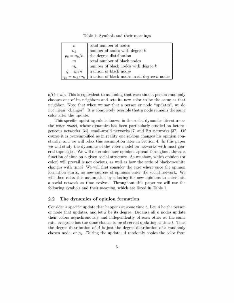
Table 1: Symbols and their meanings

n total number of nodesnk number of nodes with degree k

pk = nk/n the degree distributionm total number of black nodesmk number of black nodes with degree k

q = m/n fraction of black nodesqk = mk/nk fraction of black nodes in all degree-k nodes

b/(b+ w). This is equivalent to assuming that each time a person randomlychooses one of its neighbors and sets its new color to be the same as thatneighbor. Note that when we say that a person or node “updates”, we donot mean “changes”. It is completely possible that a node remains the samecolor after the update.

This specific updating rule is known in the social dynamics literature asthe voter model, whose dynamics has been particularly studied on hetero-geneous networks [34], small-world networks [7] and BA networks [37]. Ofcourse it is oversimplified as in reality one seldom changes his opinion con-stantly, and we will relax this assumption later in Section 4. In this paperwe will study the dynamics of the voter model on networks with most gen-eral topologies. We will determine how opinions spread throughout the as afunction of time on a given social structure. As we show, which opinion (orcolor) will prevail is not obvious, as well as how the ratio of black-to-whitechanges with time? We will first consider the case where once the opinionformation starts, no new sources of opinions enter the social network. Wewill then relax this assumption by allowing for new opinions to enter intoa social network as time evolves. Throughout this paper we will use thefollowing symbols and their meaning, which are listed in Table 1.

2.2 The dynamics of opinion formation

Consider a specific update that happens at some time t. Let A be the personor node that updates, and let k be its degree. Because all n nodes updatetheir colors asynchronously and independently of each other at the samerate, everyone has the same chance to be observed updating at time t. Thusthe degree distribution of A is just the degree distribution of a randomlychosen node, or pk. During the update, A randomly copies the color from

5

one of its neighbors, which we will call B. We calculate the change of mk

due to this specific update. There are three cases:

1. A is white and B is black. A updates its color to black and conse-quently increases mk by 1.

2. A is black and B is white. A updates its color to white and conse-quently decreases mk by 1.

3. A and B have the same color. In this case mk does not change.

Given A’s degree k, the probability that A is black or white before the updateis simply qk or 1 − qk by definition. To calculate the black probability ofB we need to know its degree distribution first, which in our case is notpk. This is because A being a randomly chosen node is more likely to be aneighbor of a high degree node than a low degree node. Specifically, underthe uniform connection assumption, the probability that B has degree j isproportional to jpj [15]. Conditioning on the event that B has degree j,the black probability of B is again simply qj . Thus, the probability that theupdate changes a degree-k node from white to black (case 1) is given by

Pw→b(k) = pk(1 − qk)

∑

j jpjqj∑

j jpj. (1)

Similarly, the probability that the update changes a degree-k node fromblack to white (case 2) is given by

Pb→w(k) = pkqk

∑

j jpj(1 − qj)∑

j jpj= pkqk

(

1 −∑

j jpjqj∑

j jpj

)

. (2)

If we define

〈q〉 =

∑

j jpjqj∑

j jpj(3)

to be a weighted average over all qk’s, then the two probabilities can bewritten as

Pw→b(k) = pk(1 − qk)〈q〉, (4)

Pb→w(k) = pkqk(1 − 〈q〉). (5)

This gives us the increment of mk due to a particular update:

∆mk =

+1 with probability pk(1 − qk)〈q〉−1 with probability pkqk(1 − 〈q〉)

0 otherwise. (6)

6

Note that the updating process of the whole network (not just one node) isa Poisson process of rate nλ. Hence the increment of mk in a time interval(t, t + dt) is given by

∆mk =

+1 with probability nk(1 − qk)〈q〉λdt−1 with probability nkqk(1 − 〈q〉)λdt

0 otherwise, (7)

where we used the fact nk = npk. We can now calculate the expectationand variance of the random variable ∆mk. Its expectation is given by

E[∆mk] = nk(1 − qk)〈q〉λdt − nkqk(1 − 〈q〉)λdt = nk(〈q〉 − qk)λdt. (8)

Its second moment is equal to

E[(∆mk)2] = nk(1 − qk)〈q〉λdt + nkqk(1 − 〈q〉)λdt

= nk(〈q〉 + qk − 2〈q〉qk)λdt. (9)

Hence the variance is given by

var[∆mk] = E[(∆mk)2] − (E[∆mk])

2

= nk(〈q〉 + qk − 2〈q〉qk)λdt + o(dt)

= nkσ2kλdt + o(dt), (10)

whereσ2

k ≡ 〈q〉 + qk − 2〈q〉qk. (11)

By definition, qk = mk/nk, so we have (to dt order)

E[∆qk] =1

nkE[∆mk] = (〈q〉 − qk)λdt, (12)

and

var[∆qk] =1

n2k

var[∆mk] =1

nkσ2

kλdt. (13)

The increment step of ∆qk is 1/nk. When n is large this step is small, andEq. (12) and (13) can be approximated by a continuous process describedby the following stochastic differential equation

dqk = (〈q〉 − qk)λdt +1√nk

σk

√λdB

(k)t , (14)

where B(k)t are k independent Brownian motions. From now on we redefine

the time unit so that λ = 1. Then Eq. (14) becomes

dqk = (〈q〉 − qk)dt +1√nk

σkdB(k)t . (15)

which is the set of equations that governs the dynamics of the social network.

7

2.3 The solution

2.3.1 Martingale

The quantities qk and 〈q〉 in Eq. (15) are all random variables, and σk isnonlinear in qk. As a result Eq. (15) is very hard to solve. However, observethat if we take the weighted average (see Eq. (3)) of both sides of Eq. (15),we obtain

d〈q〉 = 〈 1√nk

σkdB(k)t 〉, (16)

or

〈q(t)〉 =

∫ t

0〈 1√

nkσkdB(k)

s 〉 =

(

∑

k

kpk

)

−1∑

k

kpk√nk

∫ t

0σkdB(k)

s . (17)

Because the right hand side does not include the dt term, 〈q〉 is a martingale.Thus its expectation value does not change with time1:

E[〈q(t)〉] = constant. (18)

Note that 〈q(t)〉 is a positive martingale bounded by 1. From the continuous-time martingale convergence theorem [24] it follows that 〈q(t)〉 converges to astable distribution as t → ∞. It is easy to check that the only two absorbingstates are all black and all white, so the stable distribution is described byP (all black) = E[〈q(0)〉] and P (all white) = 1 − E[〈q(0)〉].

2.3.2 The large n limit

When n is large n−1/2k is small, so that we can neglect the fluctuation term

in Eq. (15) and writedqk

dt= 〈q〉 − qk. (19)

This amounts to a mean-field approximation. We divide the nodes intodifferent groups according to their degrees, so that all nodes in the samegroup have the same degree. If when n is large the size nk of each groupis also large, then we can approximately neglect the fluctuations withineach group and replace the group-wise random variables mk, qk by theirmean values. In this sense Eq. (19) can be regarded as a set of normaldifferential equations which contain deterministic variables only. Since 〈q〉is now deterministic, Eq. (18) becomes

〈q〉 = constant. (20)

1This conservation law is independently reported in [37].

8

Thus Eq. (19) can be easily solved. The solution is

qk(t) = qk(0)e−t + 〈q(0)〉(1 − e−t). (21)

We see that for each k,limt→∞

qk(t) = 〈q〉. (22)

Because q =∑

nkqk/∑

nk is a simple average over qk, we have from Eq. (21)

q(t) = q(0)e−t + 〈q(0)〉(1 − e−t) (23)

andlimt→∞

q(t) = 〈q〉. (24)

2.3.3 The convergence time

Based on a conservation result similar to that given in Section 2.3.1, Soodand Redner [34] estimated the convergence time of voter models on heteroge-neous graphs. They showed that for a network of n nodes with an arbitrarybut uncorrelated degree distribution (same as our assumption), the meantime to reach consensus Tn scales as nµ2

1/µ2, where µk is the kth moment ofthe degree distribution. Thus on a regular graph with O(1) degree Tn ∼ n.On a scale-free graph with degree distribution pk ∼ k−α, Tn scales as

Tn ∼

n α > 3,n/ log n α = 3,

n(2α−4)/(α−1) 2 < α < 3,(log n)2 α = 2,O(1) α < 2.

(25)

We see that in most cases Tn diverges as n diverges. As we will also see inSection 2.5, on average each node switches its color many times before thewhole system reaches consensus, which means that the convergence time canbe so long that in practice a consensus may not even be observed. [7, 37]also provide explicit evidences showing that the characteristic stabilizationtime diverges with the system size.

2.4 Interpretation of the solution

A direct corollary of Eq. (18) is that if one starts with a nontrivial initialdistribution of opinions (i.e., the nodes are not all black or all white), thenthe long-term stable distribution will not be trivial. This rather surprising

9

result was tested in a computer experiment described in Section 2.5. Ingeneral the overall fraction of black nodes q is not equal to 〈q〉, so it canchange with time. Eq. (24) shows that q approaches 〈q〉 as time goes on.To put it more clearly, suppose at t = 0 the network is colored in some waysuch that q 6= 〈q〉, then averagely speaking, as time passes 〈q〉 stays at itsinitial value, while q keeps moving towards 〈q〉. This is also confirmed bysimulation. To better compare q and 〈q〉 we rewrite their definitions as

q =m

n=

∑

mk∑

nk; (26)

〈q〉 =

∑

kpkqk∑

kpk=

∑

knkqk∑

knk=

∑

kmk∑

knk. (27)

It becomes clear that in the weighted average 〈q〉, each node is given aweight k equal to its degree. Thus, Eq. (24) and (27) says that a high-degreenode contributes more to the final fraction of colors (decisions) than a low-degree node. Quantitatively, the contribution of every node is proportional

to its degree. In other words, high-degree nodes are more influential. Thisexplains why a relatively small number of people with high social rankscan affect a significant proportion of the whole society in their decisionmaking. We emphasize that our theory explains, rather than assumes whyhigh-rank nodes are more influential in affecting opinion formation than lowrank nodes. In fact, in our model when a node updates its color, it putsequal weight on all its neighbors. The chance that it will get the color froma high-degree neighbor and the chance that it will get from a low-degreeneighbor are the same. However, statistically speaking there are more nodesin the network that are affected by any high-degree node. In other words,people with higher social rank are more influential because more people pay

attention to them (more people are connected to them). Notice that thisnot the same as ascribing a higher weight to the single opinion of a high-rank member of the group. Furthermore the fragility of opinion formationthat our theory exhibits stems from the possibility that a relatively smallnumber of nodes contribute a significant proportion to the weighted 〈q〉,thus changing the whole network dramatically. This effect was also testedby computer simulations which we will show in the next section.

2.5 Computer simulations

2.5.1 Regular graph

We performed our first simulation on a regular 20 × 20 2-dimensional grid.The left edge and the right edge of the grid were connected to each other,

10

and so were the upper and lower edges. Each node in the graph had degree4. We randomly assigned 70% of the nodes to be black and 30% to be white.We then randomly picked one node in the network and randomly updatedits color to be the color of one of its neighbors. This “pick-and-update”step was repeated 104 times so that on average each node got updated 25times. We then recorded the final q (which equals 〈q〉 because the graphis regular). We repeated this experiment 100 times, each time on the samenetwork but with a different initial assignment of colors. The average Eqtaken over the 100 experiments (each run for 104 steps) was 69.72%, whichverified the conservation of E〈q〉.

It is worth noting that none of the 100 experiments reached consensusafter 104 steps, showing that it takes a long time for the system to stabilize.

2.5.2 Random colored scale-free network

The results derived in the previous sections apply to arbitrary degree dis-tributions. In order to stress the degree effect, we performed our rest sim-ulations on a connected power-law network of size n = 104 and α = 2.7,whose (continuous) degree distribution is given by pk = (α − 1)k−α, k ≥ 1.A sample degree distribution for such a network is shown in Fig. 1.

We first created a random network as described and randomly assigned70% of the nodes to be black and 30% to be white. We then repeated the“pick-and-update” step 106 times so that on average each node got updated100 times, which is a rather large number for a network of this size. These106 steps constitute a “sample path” of the stochastic process, along whichboth q and 〈q〉 were calculated as functions of t. We repeated this experiment100 times, each time on regenerated networks, so that 100 sample paths werecollected. Three of those sample paths are shown in Fig. 2 and 3. As canbe seen from the figures, 〈q〉 has a larger variance than q.

It can be also seen from Fig. 2 that even after each node has updated itscolor 100 times on average, the system still has not yet reached consensus.Therefore we are able to conclude that the characteristic time for the systemto stabilize is very long. This is again consistent with the common observa-tion that conformity throughout a society tends to be localized rather thanwidespread.

If we take the average of q(t) and the 〈q(t)〉 over all 100 sample pathswe get estimates for Eq(t) and E〈q(t)〉. These are shown in Fig. 4. It isclear that both Eq and E〈q〉 do not change with time, which confirms theprediction of a martingale in Eq. (18).

11

0

1

2

3

4

5

6

7

8

9

0 1 2 3 4 5 6

log(

n k)

log(k)

degree distribution

Figure 1: Degree distribution of a network with size 104 and α = 2.7.

0

0.2

0.4

0.6

0.8

1

0 20 40 60 80 100

q

t

Figure 2: Evolution of the fraction of black nodes, q, on a scale-free randomnetwork. The unit of time, t, is 104 rounds. The three fraction curvesare calculated along three different sample paths, each path sampled on adistinct network. As can be seen none of the three curves reaches 0 or 1after 100× 104 rounds, suggesting a long characteristic time of convergence.

12

0

0.2

0.4

0.6

0.8

1

0 20 40 60 80 100

<q>

t

Figure 3: Evolution of the weighted fraction of black nodes, 〈q〉, on a freerandom network. The unit of time, t, is 104 rounds. The three weightedfraction curves are calculated along the same three sample paths as in Fig. 2.

0

0.2

0.4

0.6

0.8

1

0 20 40 60 80 100

t

EqE<q>

Figure 4: The expected fraction of black nodes (red line) and the expectedweighted fraction of black nodes (green line) do not change with time. Theexpectations are estimated by averaging over 100 sample paths.

13

0

0.2

0.4

0.6

0.8

1

0 20 40 60 80 100

q

t

Figure 5: Evolution of the fraction of black nodes, q, on a free network withthe 100 highest-degree nodes set to white. The unit of time is 104 rounds.The three fraction curves are again calculated along three sample paths onthree distinct networks.

2.5.3 Nonrandom color modification

To show that a significant proportion of nodes can be affected by a smallnumber of high-degree nodes, we performed the following experiment. Asin Section 2.5.2, we first created a random network, and then randomly as-signed 70% of its nodes to be black and 30% to be white. We then manually

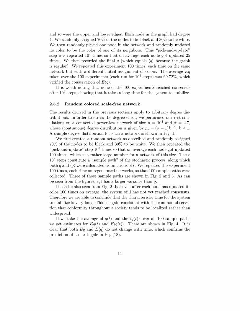
assigned the 100 highest-degree nodes to the color white. Because these 100nodes constitute only 1% of the whole network and some of them were orig-inally white before the manual assignment, only less than 1% proportion ofthe network is affected. In other words, the change of q due to the manualstep was less than 1%, which can be neglected. On the other hand, becausethe 100 high-degree nodes contribute a significant weight to the weightedaverage, the change in the value of 〈q〉 is significant and cannot be neglected.In fact, 〈q〉 was lowered from 0.7 to about 0.55 by the color modification.The rest steps remain the same as in Section 2.5.2. We again collected 100sample paths, three of which are shown in Fig. 5 and 6.

We also take the sample averages of q and 〈q〉 and plot them as functionsof time (Fig. 7). It can be seen that E〈q〉 again does not change with time,which further confirms Eq. (18). It is also seen that Eq approaches E〈q〉 as

14

0

0.2

0.4

0.6

0.8

1

0 20 40 60 80 100

<q>

t

Figure 6: Evolution of the weighted fraction of black nodes, 〈q〉, on a freenetwork with the 100 highest-degree nodes set to white. The unit of time is104 rounds. The three fraction curves are calculated along the same threesample paths as in Fig. 5.

time goes on, as predicted by Eq. (24).

3 Social networks with a sprinkle of fixed opinions

3.1 Dynamical equations

So far we have assumed that the network is free in the sense that everyperson-node can change its color at will any number of times. We nowextend our model to allow a fraction of the people to have fixed opinions,which translates into nodes with fixed colors. These recalcitrant people ornodes can be regarded as “sources” of the network, in the sense that theycan affect others but they themselves cannot be affected by the opinion ofothers. In a social context, these nodes correspond to “decided” people whilethe other nodes correspond to “undecided” people. Let bk be the proportionof degree-k nodes that stay black forever, and let wk be the proportion ofdegree-k nodes that stay white forever. The remaining 1−bk−wk proportionof degree-k nodes are free to change their colors as before. We now studywhat the final outcome is going to be for this more realistic case. The

15

0

0.2

0.4

0.6

0.8

1

0 20 40 60 80 100

t

EqE<q>

Figure 7: Evolution of the expected value of the fraction of black nodes, Eq,towards the expected weighted fraction E〈q〉 as a function of time. At thebeginning Eq = 0.7 and E〈q〉 = 0.55. The equilibrium Eq = E〈q〉 = 0.55 isreached after about 10 × 104 rounds, i.e., after each node updates its color10 times on average.

16

difference between a free network and a network with sources is that in thelatter case when we randomly choose a node to update, we have to makesure it is free and thus can be updated. Suppose a degree-k node is chosen.At the moment it is chosen, there are nk(1− qk) white nodes with degree k,among which nkwk are not free. Therefore the probability that a free whitenode is chosen is

nk(1 − qk) − nkwk

nk= 1 − qk − wk. (28)

Hence we need to replace 1 − qk by 1 − qk − wk in Eq. (4) to obtain

Pw→b(k) = pk(1 − qk − wk)〈q〉, (29)

Similarly, Eq. (5) is modified to

Pb→w(k) = pk(qk − bk)(1 − 〈q〉). (30)

Repeating the steps in the previous section, we can reach a set of dynamicalequations similar to Eq. (15):

dqk = [〈q〉 − qk + bk(1 − 〈q〉) − wk〈q〉]dt +1√nk

σkdB(k)t , (31)

where σk is a complicated function of qk which we do not write out. Whenbk = wk = 0 Eq. (31) becomes Eq. (15).

3.2 The solution

Taking the weighted average on both sides of Eq. (31), we have

d〈q〉 = [bk(1 − 〈q〉) − wk〈q〉]dt + 〈 1√nk

σkdB(k)t 〉. (32)

Hence 〈q〉 is no longer a martingale. If we again apply the mean-field ap-proximation to neglect the fluctuation terms, we get

d〈q〉dt

= 〈b〉(1 − 〈q〉) − 〈w〉〈q〉. (33)

The equilibrium condition is obtained by setting the right hand side equalto zero (q∞ = q(t = ∞)):

〈b〉(1 − 〈q∞〉) − 〈w〉〈q∞〉 = 0, (34)

17

which gives

〈q∞〉 =〈b〉

〈b〉 + 〈w〉 . (35)

Therefore as t → ∞, 〈q(t)〉 converges to a fixed fraction equal to the weightedproportion of non-free black nodes among all non-free nodes. We see thatthe final proportion does not depend on the random initial assignment of thecolors of the free nodes, although it is possible that the convergence needssuch a long time that it can never be reached in reality. Anyway, Eq. (35)shows that the weighted average again plays an important role, indicatingthat high-degree nodes are more influential to the final outcome.

4 The effect of undecided individuals

4.1 Model

In the first two models we assumed that each person or node can make deci-sions repeatedly for any number of times. However, in some circumstances,once a node makes a decision it remains unchanged during the whole pro-cess of opinion formation. Accordingly, we will now assume that there aretwo kinds of people or nodes, decided and undecided. A decided node hasopinion either black or white, which does not change with time, while anundecided node has no color at the beginning but can obtain one from oneof his neighbors after an update of its state. Once it gets a color, it becomesdecided and its color stays fixed forever. To conclude, each node has threepossible states: black, white and undecided. As before, at each step werandomly pick a node from the network and check its state. If it alreadyhas a color (decided), we do nothing. If it is undecided, we randomly pickone of its neighbor. If that neighbor is also undecided, we again do nothing,otherwise we update the first node’s color to be the same as its neighbor’s.

4.2 Solution

Let bk and wk be the proportion of black and white nodes in the network,respectively. e assume that bk + wk < 1 at t = 0 so that there are a finitenumber of undecided nodes at the beginning. We calculate the probabilitythat the number of k-degree black nodes will be increased by one duringan update. For this to happen, first we have to choose an undecided nodein step 1, which happens with probability 1 − bk − wk, and then its neigh-bor we choose in step 2 has to be black, which happens with probability

18

∑

kpkbk/∑

kpk. Thus we have (again neglecting the fluctuation term bymean-field approximation)

dbk

dt= (1 − bk − wk)〈b〉, (36)

and similarlydwk

dt= (1 − bk − wk)〈w〉. (37)

Eq. (36) and (37) govern the dynamics of the system. Taking the weightedaverage of Eq. (36) and (37), we obtain

d〈b〉dt

= (1 − 〈b〉 − 〈w〉)〈b〉, (38)

andd〈w〉dt

= (1 − 〈b〉 − 〈w〉)〈w〉. (39)

To solve Eq. (38) and (38), we take their sum and define f = 1 − 〈b〉 − 〈w〉to get

df

dt= f(1 − f). (40)

Now f can be solve as

f(t) =1 − f0

f0et + 1 − f0, (41)

where f0 = f(0) = 1 − 〈b(0)〉 − 〈w(0)〉. Putting this back into Eq. (38) and(39), we can solve out 〈b〉 and 〈w〉, which we write down here:

〈b〉 =〈b(0)〉et

f0et + 1 − f0, 〈w〉 =

〈w(0)〉et

f0et + 1 − f0. (42)

Hence〈b(t)〉〈w(t)〉 =

〈b(0)〉〈w(0)〉 = const. (43)

We see that the weighted black-to-white ratio does not change with time. Infact, this can be seen from Eq. (38) and (39) directly, where the incrementsof 〈b〉 and 〈w〉 is proportional to 〈b〉 and 〈w〉, respectively.

19

5 Information asymmetries

The updating rule of the voter model is linear in the sense that the probabil-ity that a node will update its color to black is proportional to the numberof its black neighbors. This is of course a simplification, as in real worldhigh degree nodes are usually more immune to influence by a single inno-vating neighbor. A possible extension of our model is to assume a moregeneral updating rule. Such an extension, however, will probably break upthe martingale property and we are not going to pursue it here.

Another possible way to extend our model is to incorporate informationalasymmetries into our assumptions in such a way that it is possible for Ato get information from B but B cannot get information from A. Thiscorresponds to the study of our model on a directed graph and is illustratedin Fig. 8. In this example B,C,D,E can get information from A but Acan only get information from D. A directed graph resembles more closelya real life social network, in which low-rank people pay more attention tohigh-rank people than the other way around. To generalize our model forundirected graphs, from the point of view of our notation we need to do isto replace the numerous appearances of “degree” by “outgoing degree” inTable 1. As an example, pk now stands for “outgoing degree distribution”.We point out that the outgoing degree distribution of a directed graph canbe very different from the degree distribution of the same graph viewed asan undirected graph. For example, node D in Fig. 1 has outgoing degree2 as a directed graph but degree 3 as an undirected graph. Under the newdefinition, all our previous results still hold.

6 Discussion

In this paper we presented a theory of opinion formation that explicitlytakes into account the structure of the social network in which individualsare embedded. The theory assumes asynchronous choices by individualsamong two or three opinions and it predicts the time evolution of the set ofopinions from any arbitrary initial condition. We showed that under verygeneral conditions a martingale property ensues, i.e. the expected weightedfraction of the population that holds a given opinion is constant in time.By weighted fraction we mean the fraction of individuals holding a givenopinion, averaged over their social connectivity (degree).2

2Note that in the context of epidemic control Dezso and Barabasi established a similarresult that it is more efficient to cure the high degree nodes first [10, 11]. However, they

20

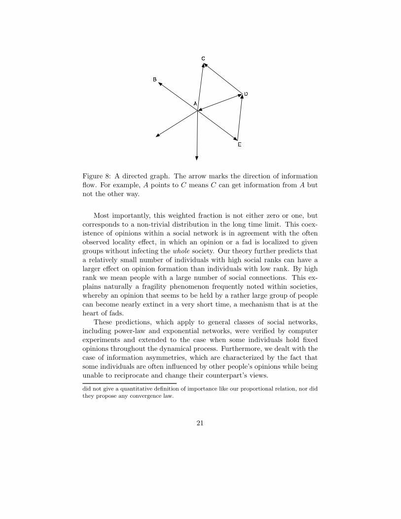
Figure 8: A directed graph. The arrow marks the direction of informationflow. For example, A points to C means C can get information from A butnot the other way.

Most importantly, this weighted fraction is not either zero or one, butcorresponds to a non-trivial distribution in the long time limit. This coex-istence of opinions within a social network is in agreement with the oftenobserved locality effect, in which an opinion or a fad is localized to givengroups without infecting the whole society. Our theory further predicts thata relatively small number of individuals with high social ranks can have alarger effect on opinion formation than individuals with low rank. By highrank we mean people with a large number of social connections. This ex-plains naturally a fragility phenomenon frequently noted within societies,whereby an opinion that seems to be held by a rather large group of peoplecan become nearly extinct in a very short time, a mechanism that is at theheart of fads.

These predictions, which apply to general classes of social networks,including power-law and exponential networks, were verified by computerexperiments and extended to the case when some individuals hold fixedopinions throughout the dynamical process. Furthermore, we dealt with thecase of information asymmetries, which are characterized by the fact thatsome individuals are often influenced by other people’s opinions while beingunable to reciprocate and change their counterpart’s views.

did not give a quantitative definition of importance like our proportional relation, nor didthey propose any convergence law.

21

While the assumption of only two or three opinions within a social net-work may seem restrictive, there are many real world instances where peoplebasically choose among points of view. Examples are the choice among twoprevalent technologies [33, 25], elections in two party systems, managementfads which consultants and executives need to decide whether to implementor not, and highly polarized attitudes towards government actions in manysocial settings. Our finding that social structure and ranking do affect theformation of these opinions and that they can coexist with each other are inagreement with many empirical observations. Our findings also cast doubton the applicability of tipping models to a number of consumer behaviors[21]. While there are clear thresholds in the spread of innovations whennetwork externalities are at play [33, 22, 27] it is not clear that the samephenomenon is observed in situations where externalities are not at play. Inmost of the consumer behaviors that have been “explained” by tipping pointideas one still observes the coexistence of the old and the new preference oropinions over long times, in contrast with the sudden onset seen in the caseof positive externalities.

We thank Lada Adamic, Phillip Bonacich and Chenyang Wang for usefulsuggestions.

References

[1] E. Abrahamson and L. Rosenkopf, Social network effects on the extentof innovation diffusion: A comupter simulation, Org. Sci. 8 (3) 289–309(1997).

[2] P. Anderson and M. L. Tushman, Technological discontinuities anddominant designs, Admin. Sci. Quarterly 35 604–633 (1993).

[3] A. Barabasi and R. Albert. Emergence of scaling in random networks.Science, 286 509–512 (1999).

[4] S. Bikhchandani, D. Hirshleifer and I. Welch, A theory of fads, fash-ion, custom, and cultural change as informational cascades, Journal ofPolitical Economy 100(5), 992–1026 (1992).

[5] S. Bikhchandani, D. Hirshleifer and I. Welch, Learning from the behav-ior of others: conformity, fads, and informational cascades, Journal ofEconomic Perspectives, 12, 151–170 (1998).

22

[6] C. Camerer, Individual Decision Making. In Handbook of experimen-tal economics, Kagel and Roth (Eds.), Princeton, Princeton UniversityPress, 587–703 (1995).

[7] C. Castellano, D. Vilone and A. Vespignani, Incomplete ordering ofthe voter model on small-world networks, Europhys. Lett., 63 (1), pp.153–158 (2003).

[8] R. David, The web of politics: the Internet’s impact on the Americanpolitical system, New York, Oxford University Press (1999).

[9] G. Deffuant, D. Neau, F. Amblard and G. Weisbuch, Mixing beliefsamong interacting agents, Advances in Complex Systems, 3, 87–98(2001).

[10] Z. Dezso and A. L. Barabasi, Halting viruses in scale-free networks,Phys. Rev. E 65 (2002).

[11] P. S. Dodds and D. J. Watts, Universal behavior in a generalized modelof contagion, Phys. Rev. Lett. 92(21) 218701 (2004).

[12] J. R. P. French, A formal theory of social power, Psychological Review,Vol. 63, 181–194 (1956).

[13] N. E. Friedkin and E. C. Johnsen. Social influence and opinions. Journalof Mathematical Sociology 15: 193–205 (1990).

[14] N. E. Friedkin and M. Granovetter. A structural theory of social influ-ence. Cambridge University Press (1998).

[15] S. Feld, Why your friends have more friends than you do, Am. J. Social.,96, 1464–1477 (1991).

[16] S. Fortunato, Damage spreading and opinion dynamics on scale freenetworks, Physica A, Volume 348, pp. 683–690 (2004).

[17] S. Galam, Rational group decision making: a random field Ising modelat T = 0, Physica A 238, 66–80 (1997).

[18] S. Galam, B. Chopard, A. Masselot and M. Droz, Competing speciesdynamics: qualitative advantage versus geography, Eur. Phys. B 4,529–531 (1998).

[19] S. Galam, Application of statistical physics to politics, Physica A 274,132–139 (1999).

23

[20] S. Galam, Modelling rumors: the no plane Pentagon French hoax case,Physica A 320, 571–580 (2003).

[21] M. Gladwell, The tipping point: how little things can make a difference,Little and Brown (2002).

[22] M. Granovetter, Threshold models of collective behavior, Amer. J. So-ciology 83 1420–1443 (1978).

[23] R. Hegselmann and U. Krause, Opinion dynamics and bounded confi-dence models, analysis, and simulation, Journal of Artificial Societiesand Social Simulation, Vol. 5, No. 3 (2002).

[24] I. Karatzas and S. E. Shreve, Brownian motion and stochastic calculus,2nd Ed., pp. 17, Theorem 3.15, Springer (1997).

[25] U. Kumar and V. Kumar, Technological innovation diffusion: The pro-liferation of substitution models and easing the user’s dilemma, IEEETrans. Engrg. Management 39 158–168 (1992).

[26] M. F. Laguna, S. Risau-Gusman, G. Abramson, S. Goncalves, and J. R.Iglesias, The dynamics of opinion in hierarchical organizations, PhysicaA, Volume 351, Issues 2–4 , pp. 580–592 (2004).

[27] C. Loch and B. A. Huberman, Punctuated equilibrium model of tech-nology diffusion, Management Science, Vol. 45, 160–177 (1999).

[28] M. Margolis and D. Resnick, Politics as usual: the cyberspace ”revolu-tion.”, Thousand Oaks, CA, Sage (2000).

[29] R. Milo, N. Kashtan, S. Itzkovitz, M. E. J. Newman, and U. Alon.On the uniform generation of random graphs with prescribed degreesequences. oai:arXiv.org:cond-mat/0312028 (2003).

[30] M. E. J. Newman, S. H. Strogatz and D. J. Watts, Random graphs witharbitrary degree distributions and their applications, Phys. Rev. E, 64,041902 (2001).

[31] W. Rash, Politics on the nets: wiring the political process. New York,Freeman (1997).

[32] H. Rheingold, The virtual community: homesteading on the electronicfrontier, Reading, MA, Addison-Wesley (1993).

24

[33] E. M. Rogers, The “critical mass” in the diffusion of interactive tech-nologies in organizations, K. L. Kraemer ed., The information systemsresearch challenge: survey research methods, Chapter 8, Harvard Busi-ness School Press, Boston MA, 245–271 (1991).

[34] V. Sood and S. Redner, Voter model on heterogeneous graphs,Phys. Rev. Lett. 94, 178701 (2005).

[35] D. Stauffer and H. Meyer-Ortmanns, Simulation of consensus model ofDeffuant et al on a Barabasi-Albert network, Int. J. Mod. Phys. C 15,2 (2003).

[36] D. Stauffer, A. O. Sousa and C. Schulze, Discretized opinion dynamicsof Deffuant model on scale free networks, Journal of Artificial Societiesand Social Simulation, vol. 7, no. 3 (2004).

[37] K. Suchecki, V. M. Eguiluz and M. S. Miguel, Conservation laws for thevoter model in complex networks, Europhys. Lett., 69(2), pp. 228–234(2005).

[38] K. Sznajd-Weron and J. Sznajd, Opinion evolution in closed commu-nity, Int. J. Mod. Phys. C 11, 6 (2000).

[39] C. J. Tessone, R. Toral, P. Amengual, M. San Miguel, and H. Wio,Neighborhood models of minority opinion spreading, Eur. Phys. J. B39, 4, pp. 535–544 (2004).

[40] D. J. Watts. A simple model of global cascades on random networks.PNAS Vol. 99, 9, 5766–5771 (2002).

[41] A. G. Wilheim, Democracy in the digital age: challenges to politicallife in cyberspace, New York, Routledge (2000).

25