social power dynamics over switching and stochastic ...motion.me.ucsb.edu/pdf/2016j-cdfb.pdf ·...

0018-9286 (c) 2018 IEEE. Translations and content mining are permitted for academic research only. Personal use is also permitted, but republication/redistribution requires IEEE permission. Seehttp://www.ieee.org/publications_standards/publications/rights/index.html for more information.

This article has been accepted for publication in a future issue of this journal, but has not been fully edited. Content may change prior to final publication. Citation information: DOI 10.1109/TAC.2018.2822182, IEEETransactions on Automatic Control

1

Social Power Dynamics over Switching andStochastic Influence Networks

Ge Chen, Member, IEEE, Xiaoming Duan, Noah E. Friedkin, Francesco Bullo, Fellow, IEEE

Abstract—The DeGroot-Friedkin (DF) model is a recently-proposed dynamical description of the evolution of individuals’self-appraisal and social power in a social influence network.Most studies of this system and its variations have so far focusedon models with a time-invariant influence network.

This paper proposes novel models and analysis results forDF models over switching influence networks, and with orwithout environment noise. First, for a DF model over switchinginfluence networks, we show that the trajectory of the socialpower converges to a ball centered at the equilibrium reachedby the original DF model. For the DF model with memory onrandom interactions, we show that the social power convergesto the equilibrium of the original DF model almost surely.Additionally, this paper studies a DF model which containsrandom interactions and environment noise, and has memoryon the self-appraisal. We show that such a system converges toan equilibrium or a set almost surely. Finally, as a by-product, weprovide novel results on the convergence rates of the original DFmodel and convergence results for a continuous-time DF model.

Index Terms—DeGroot-Friedkin model, stochastic approxima-tion, social networks, social power evolution, opinion dynamics

I. INTRODUCTION

Models for the dynamics of opinions and social power:Over the past decades, social networks have drawn tremendousattention from both academia and industry. The study ofopinion dynamics aims to characterize and understand howindividuals’ opinions form and evolve over time throughinteractions with their peers. The first mathematical modelfor opinion dynamics was proposed by French in [9] withfurther refinements by Harary [16]. This model is based ondistributed opinion averaging and is now widely referred to asthe DeGroot model [8]. Closely-related important variationsinclude the Friedkin-Johnsen affine model [12], [13] and theHegselmann-Krause bounded-confidence model [17].

This material is based upon work supported by, or in part by, the U.S.Army Research Laboratory and the U.S. Army Research Office under grantnumber W911NF-15-1-0577. The research of G. Chen was supported in partby the National Natural Science Foundation of China under grants 91427304,61673373 and 11688101, the National Key Basic Research Program of China(973 program) under grant 2014CB845301/2/3, and the Leading researchprojects of Chinese Academy of Sciences under grant QYZDJ-SSW-JSC003.

Ge Chen is with the NCMIS and the LSC, Academy of Mathematics andSystems Science, Chinese Academy of Sciences, Beijing 100190, China,[email protected]

Xiaoming Duan and Francesco Bullo are with the Departmentof Mechanical Engineering and the Center of Control, Dynamical-Systems and Computation, University of California at Santa Barbara,CA 93106-5070, USA. [email protected];[email protected]

Noah E. Friedkin is with the Department of Sociology and the Center ofControl, Dynamical-Systems and Computation, University of California atSanta Barbara, CA 93106, USA. [email protected]

Recently, by combining the DeGroot model of opinion dy-namics and a reflected appraisal mechanism [6], [10], Jia et al.[20] proposed a DeGroot-Friedkin (DF) model to describe theevolution of individuals’ self-appraisal and social power (i.e.,influence centrality) along an issue sequence. This influencenetwork model combines two steps. First, individuals updatetheir opinions on each issue as in the DeGroot averagingmodel, where an interaction matrix characterizes the relativeinterpersonal influence among the individuals. Second, basedon the opinion averaging outcome, individuals update theirself-appraisal via a reflection appraisal mechanism. In otherwords, individuals’ self-appraisals on the current issue are el-evated or dampened depending upon their influence centrality(i.e., social power) on the prior issue. Under an assumptionthat the relative interaction matrix is constant, irreducible,and row-stochastic, Jia et al. [20] proved the convergence ofindividuals’ self-appraisals in the DF model.

Since its introduction, the DF model has attracted a lotof interest. Two articles study the DF model with varyingassumptions on the interaction matrix. First, Jia et al. [19]extend the convergence results to the setting of reducibleinteraction matrices. Second, Ye et al. [27] show that, if theinteraction matrix switches in a periodic manner, then indi-viduals’ self-appraisals have a periodic solution. Additionally,several other dynamical models have been proposed and ana-lyzed. Mirtabatabaei et al. extended the DF model to includestubborn agents who have attachment to their initial opinionsin [22]. Xu et al. [26] proposed a modified DF model, wherethe social power is updated without waiting for the opinionconsensus on each issue, i.e., the local estimation of socialpower is truncated; a complete analysis of convergence andequilibria properties was given when the interaction matrix isdoubly stochastic. Considering time-varying doubly stochasticinfluence matrix, Xia et al. [25] investigated the convergencerate of the modified DF model, which was proven to convergeexponentially fast. A continuous-time self-appraisal model wasintroduced by Chen et al. in [4]. It is worth noting that, allthe above existing works assume the interaction matrix eitheris constant or has some special time-varying structure, likedouble stochasticity or periodicity [25], [27].

Empirical evidence motivating new models: Empiricalevidence in support of the DeGroot model for opinion dy-namics is provided in [2] and support of the reflected appraisalmechanism over issue sequences is provided in [10], [11]. Thedata in [11] establishes that (i) the interaction matrix in theinfluence network is not constant along the issue sequence, (ii)the reflected appraisal mechanism is indeed observed, wherebyprior influence centrality predict future self-appraisals, and



2

(iii) a predictor of self-appraisal that is even better than priorsocial power is cumulative prior social power (i.e, the averageof prior influence centrality scores over the issue sequence).In other words, individuals learn “their place in a socialgroup” via an accumulation of experiences rather than overa single episode. It is worth mentioning that a similar learningmechanism based on the averages of prior outcomes is widelyadopted [18] in game theory and economics to model humanbehavior.

Motivated by the available empirical evidence, this paperproposes and characterizes several DF models subject toswitching influence networks, and also the environment noise.Additionally, we incorporate memory in our models so that,for example, individuals may update their self-appraisal basedon cumulative prior influence centrality.

Useful tools: In what follows, we adopt useful stochasticmodels and analysis methods from the field of stochasticapproximation; these models and methods were originallyaimed at optimization and root-finding problems with noisydata. The earliest methods of stochastic approximation wereproposed by Robbins and Monro [23] and aimed to solvea root finding problem. During more than sixty years ofdevelopment, stochastic approximation methods have attracteda lot of interest due to many applications such as the studyof reinforcement learning [24], consensus protocols in multi-agent systems [3], and fictitious play in game theory [18].For general noisy processes and algorithms, a very powerfulstochastic approximation tool is the so-called “ordinary differ-ential equations (ODE) method” (see Chapter 5 in [21]), whichtransforms the analysis of asymptotic properties of a discrete-time stochastic process into the analysis of a continuous-timedeterministic process.

Statement of contributions: This paper proposes and an-alyzes multiple novel DF models with varying assumptions oninteraction and memory. First, we investigate a DF model withswitching interactions, i.e., we assume that the interpersonalinteraction matrix is time-varying. Under such a model, weestablish convergence results under both relevant settings, i.e.,when the digraph corresponding to the interaction matrix is oris not a star graph. In the former case, the trajectory of socialpower converges to autocracy; in the latter case, the socialpower converges into a ball centered at the equilibrium pointreached by the original DF model. Second, as a by-product ofthis analysis, we establish convergence rates for the originalDF model for both settings (with or without star topology).

Third, we consider a DF model with memory on the randominteraction matrix. In such a model the self-appraisal of eachindividual is updated in the same manner as that in the originalDF model, but we assume the individual has memory onthe interaction weights assigned to others. For such a modelwe show, using a stochastic approximation method, that theimpact of the stochasticity on the interaction matrix disappearsasymptotic. In other words, we prove that, for this model, thesocial power converges to the same equilibrium point reachedby the original DF model almost surely.

Fourth, we study a DF model which contains random inter-actions and environment noise, and has memory on the self-appraisal. In this model, each individual remembers his/her

self-appraisal of last time (modeling for example the conceptof cumulative prior social power). While this model is quitedifferent from the DF model with memory on the interactionmatrix, we again establish using stochastic approximationmethods (and under certain technical conditions) that theadoption of memory leads to a vanishing effect of switch andnoise and that the system converges to an equilibrium pointor a set almost surely. Fifth and finally, we also propose andcharacterize a novel continuous-time DF model.

Organization: We review the original DF model in Sec-tion II. Section III contains the convergence rate results forthe DF model and a new continuous-time DF model. Wepropose the DF models with switching and stochastic inter-actions in Section IV. A DF model with random interactions,environment noise, and self-appraisal memory is analyzed inSection V. Section VI concludes the paper.

Notations: A nonnegative matrix is row-stochastic (resp.doubly stochastic) if its row sums are equal to 1 (resp., itsrow and column sums are equal to 1). The digraph G(M)associated to a nonnegative matrix M = miji,j∈1,...,nis defined as follows: the node set is 1, . . . , n; there is adirected edge (i, j) from node i to node j if and only ifmij > 0. The nonnegative matrix M is irreducible if itsassociated digraph is strongly connected. The n-simplex ∆n

is x ∈ [0, 1]n |∑ni=1 xi = 1 and its interior is ∆o

n = x ∈(0, 1)n |

∑ni=1 xi = 1. Let ei ∈ Rn be the row vector whose

i-th component is 1 and whose other components are 0. Forv ∈ Rn, let ‖v‖∞ := max1≤i≤n |vi| denote its infinity norm.For a matrix M ∈ Rn×n, let ‖M‖max := max1≤i,j≤n |Mij |denote the maximum norm. Given two sequences of positivenumbers g1(t) and g2(t), we say g1(t) = o(g2(t)) iflimt→∞ g1(t)/g2(t) = 0, and g1(t) = O(g2(t)) if there existtwo positive constants a and t0 such that g1(t) ≤ ag2(t) forall t ≥ t0. Let Z≥0 denote the set of nonnegative integers.

II. REVIEW OF ORIGINAL DF MODEL

The original DF model was proposed by Jia et al. in [20].The model considers a group of n ≥ 3 individuals who discussa sequence of issues under the DeGroot model. The columnvector y(s, t) ∈ Rn denoting the individuals’ opinions overissue s evolves according to the following formula

y(s, t+ 1) = W (s)y(s, t),

where W (s) ∈ Rn×n is a row-stochastic influence matrix overissue s. Then, for each individual i, her opinion is updated viaa convex combination

yi(s, t+ 1) = Wii(s)yi(s, t) +n∑

j=1,j 6=i

Wij(s)yj(s, t).

Here Wii(s) denotes the self-appraisal of individual i, andWij(s) = (1−Wii(s))Cij for all i 6= j, where the coefficientCij is the relative interpersonal weight that individual iaccords to individual j. Throughout this paper, the squarematrix C is a relative interaction matrix, that is row-stochasticand zero-diagonal.



3

Denoting Wii(s) by xi(s) for simplicity as in [20], theinfluence matrix W (s) can then be decomposed as

W (s) = diag[x(s)] + (In − diag[x(s)])C.

If W (s) is an irreducible row-stochastic matrix, accordingto Perron-Frobenius theorem W (s) has a unique dominantleft eigenvector π(W (s)) ∈ Rn, which is a row vectorsatisfying π(W (s)) = π(W (s))W (x(s)), πi(W (s)) ≥ 0 forall i ∈ 1, . . . , n, and

∑ni=1 πi(W (s)) = 1. Under some

assumptions on C, the opinion vector y(s, t) asymptoticallyreaches consensus, i.e., lim

t→∞y(s, t) = [π(W (s))y(s, 0)]1n.

Let x(s) := (x1(s), . . . , xn(s)) be a row vector. To dealwith the evolution of x(s) across issues, a reflected appraisalmechanism is adopted as follows,

x(s+ 1) = π(W (s)).

The meaning of this equation is that individuals’ self weightson current issue are their relative influence centrality (i.e., so-cial power) over prior issue. In summary, given an interactionmatrix C, the DF model is given by [20]

W (x(s)) = diag[x(s)] + (In − diag[x(s)])C,

x(s+ 1) = π(W (x(s))).(1)

We adopt the same assumptions on C as in [20], i.e.,we assume that C is irreducible. According to the Perron-Frobenius theorem, C has a unique dominant left eigenvectorc := (c1, . . . , cn) with ci > 0 for all i ∈ 1, . . . , n, and∑ni=1 ci = 1.

Lemma II.1 (Lemma 2.2 in [20]: Explicit formulation of DFmodel): Assume n ≥ 2 and C ∈ Rn×n is a row-stochastic,irreducible, and zero-diagonal matrix whose dominant lefteigenvector is c. Then, for any x ∈ ∆n, the dominant lefteigenvector of the matrix diag[x] + (In − diag[x])C is ei if x = ei for all i = 1, . . . , n,(

c11−x1

, . . . , cn1−xn

)/∑ni=1

ci1−xi otherwise.

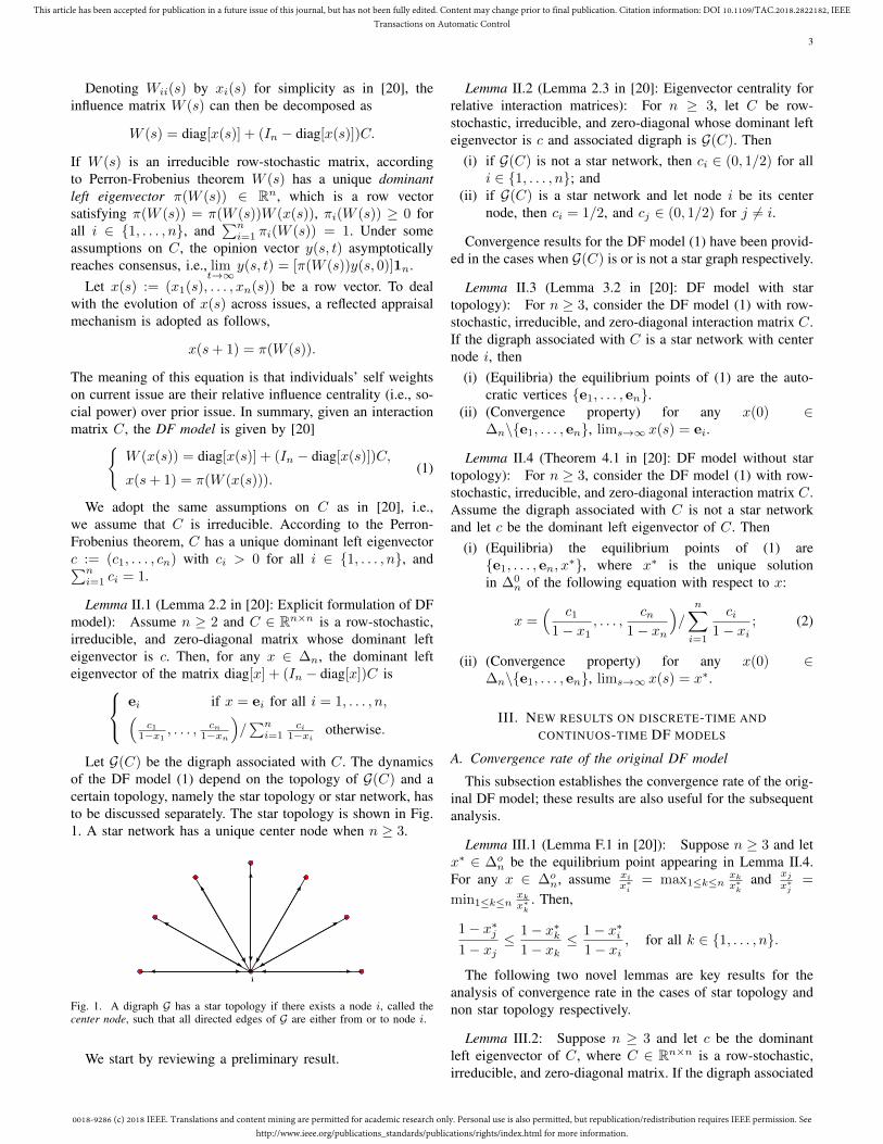
Let G(C) be the digraph associated with C. The dynamicsof the DF model (1) depend on the topology of G(C) and acertain topology, namely the star topology or star network, hasto be discussed separately. The star topology is shown in Fig.1. A star network has a unique center node when n ≥ 3.

i

Fig. 1. A digraph G has a star topology if there exists a node i, called thecenter node, such that all directed edges of G are either from or to node i.

We start by reviewing a preliminary result.

Lemma II.2 (Lemma 2.3 in [20]: Eigenvector centrality forrelative interaction matrices): For n ≥ 3, let C be row-stochastic, irreducible, and zero-diagonal whose dominant lefteigenvector is c and associated digraph is G(C). Then

(i) if G(C) is not a star network, then ci ∈ (0, 1/2) for alli ∈ 1, . . . , n; and

(ii) if G(C) is a star network and let node i be its centernode, then ci = 1/2, and cj ∈ (0, 1/2) for j 6= i.

Convergence results for the DF model (1) have been provid-ed in the cases when G(C) is or is not a star graph respectively.

Lemma II.3 (Lemma 3.2 in [20]: DF model with startopology): For n ≥ 3, consider the DF model (1) with row-stochastic, irreducible, and zero-diagonal interaction matrix C.If the digraph associated with C is a star network with centernode i, then

(i) (Equilibria) the equilibrium points of (1) are the auto-cratic vertices e1, . . . , en.

(ii) (Convergence property) for any x(0) ∈∆n\e1, . . . , en, lims→∞ x(s) = ei.

Lemma II.4 (Theorem 4.1 in [20]: DF model without startopology): For n ≥ 3, consider the DF model (1) with row-stochastic, irreducible, and zero-diagonal interaction matrix C.Assume the digraph associated with C is not a star networkand let c be the dominant left eigenvector of C. Then

(i) (Equilibria) the equilibrium points of (1) aree1, . . . , en, x

∗, where x∗ is the unique solutionin ∆0

n of the following equation with respect to x:

x =( c1

1− x1, . . . ,

cn1− xn

)/

n∑i=1

ci1− xi

; (2)

(ii) (Convergence property) for any x(0) ∈∆n\e1, . . . , en, lims→∞ x(s) = x∗.

III. NEW RESULTS ON DISCRETE-TIME ANDCONTINUOS-TIME DF MODELS

A. Convergence rate of the original DF model

This subsection establishes the convergence rate of the orig-inal DF model; these results are also useful for the subsequentanalysis.

Lemma III.1 (Lemma F.1 in [20]): Suppose n ≥ 3 and letx∗ ∈ ∆o

n be the equilibrium point appearing in Lemma II.4.For any x ∈ ∆o

n, assume xix∗i

= max1≤k≤nxkx∗k

and xjx∗j

=

min1≤k≤nxkx∗k

. Then,

1− x∗j1− xj

≤ 1− x∗k1− xk

≤ 1− x∗i1− xi

, for all k ∈ 1, . . . , n.

The following two novel lemmas are key results for theanalysis of convergence rate in the cases of star topology andnon star topology respectively.

Lemma III.2: Suppose n ≥ 3 and let c be the dominantleft eigenvector of C, where C ∈ Rn×n is a row-stochastic,irreducible, and zero-diagonal matrix. If the digraph associated



4

with C is a star network with center node i, then for anyx ∈ ∆o

n,ci

1−xi∑nj=1

cj1−xj

> xi + xi(1− xi)2(1− 2 max

j 6=icj).

Proof. By Lemma II.2 we have ci = 1/2 so that∑j 6=i cj =

1/2. Then,

ci1−xi∑nj=1

cj1−xj

=

12(1−xi)

12(1−xi) + 1

2xi+∑j 6=i

(cj

1−xj −cjxi

)=

12(1−xi)

12(1−xi)xi +

∑j 6=i

(cj

1−xj −cjxi

) . (3)

Let c′ = maxj 6=i cj . Then,∑j 6=i

( cj1− xj

− cjxi

)= −

∑j 6=i

cj(1− xi − xj)(1− xj)xi

< −∑j 6=i

cj(1− xi − xj)xi

= −1− xi2xi

+∑j 6=i

cjxjxi

≤ −1− xi2xi

+c′(1− xi)

xi= − (1− xi)(1− 2c′)

2xi.

Substituting this into (3) we have

ci1−xi∑nj=1

cj1−xj

>

12(1−xi)

12(1−xi)xi −

(1−xi)(1−2c′)2xi

=xi

1− (1− xi)2(1− 2c′)

> xi + xi(1− xi)2(1− 2c′).

(4)

Lemma III.3: Suppose n ≥ 3 and let c be the dominantleft eigenvector of C, where C ∈ Rn×n is a row-stochastic,irreducible, and zero-diagonal matrix. If the digraph associatedwith C is not a star network, then, for any x ∈ ∆o

n,

maxi6=j

ci(1− xj)x∗jcj(1− xi)x∗i

≤ 1 +

(maxi6=j

xix∗j

xjx∗i− 1

)maxi6=j

x∗i1− x∗j

,

where x∗ ∈ ∆on is the equilibrium point defined in Lemma II.4.

Proof. According to (2) we getci

(1− x∗i )x∗i=

cj(1− x∗j )x∗j

(5)

for any 1 ≤ i, j ≤ n. Hence,


=1− xj1− xi

· ci/x∗i

cj/x∗j=

1− xj1− xi

· 1− x∗i1− x∗j

. (6)

Without loss of generality, we assumex1

x∗1≤ x2

x∗2≤ · · · ≤ xn

x∗n, (7)

then by Lemma III.1, we have

1− x∗11− x1

≤ 1− x∗k1− xk

≤ 1− x∗n1− xn

, for all 1 ≤ k ≤ n.

Substituting this inequality into (6), we obtain

maxi6=j


=(1− x∗n)/(1− xn)

(1− x∗1)/(1− x1)

=1− x∗n1− x∗1

· 1− x1

1− xn.

(8)

Let δk =xk/x

∗k

x1/x∗1so that xk = δkx

∗kx1/x

∗1. By (7) we have

1 = δ1 ≤ δ2 ≤ · · · ≤ δn. Thus,

1− x1

1− xn=

∑nk=2 xk∑n−1k=1 xk

=

∑nk=2 δkx

∗k∑n−1

k=1 δkx∗k

:=z + δnx

∗n

z + x∗1, (9)

where z =∑n−1k=2 δkx

∗k. From

n−1∑k=2

x∗k ≤ z ≤ δnn−1∑k=2

x∗k,

we knowz + δnx

∗n

z + x∗1= 1 +

δnx∗n − x∗1

z + x∗1(10)

≤ 1 + max

δnx∗n − x∗1∑n−1

k=2 x∗k + x∗1

,δnx∗n − x∗1

δn∑n−1k=2 x

∗k + x∗1

= max

1− x∗1 + (δn − 1)x∗n

1− x∗n,

δn(1− x∗1)

δn(1− x∗n)− (δn − 1)x∗1

=

1− x∗11− x∗n

max

1 + (δn − 1)

x∗n1− x∗1

,δn

δn − (δn−1)x∗11−x∗n

.

Let

a∗ = maxi6=j

x∗i1− x∗j

= maxi6=j

x∗ix∗i +

∑k 6=i,j x

∗k

< 1,

so that

max

1 + (δn − 1)

x∗n1− x∗1

,δn

δn − (δn−1)x∗11−x∗n

≤ max

1 + (δn − 1)a∗,

δnδn − (δn − 1)a∗

= 1 + (δn − 1)a∗.

Substituting this inequality into (10) yields

z + δnx∗n

z + x∗1≤ 1− x∗1

1− x∗n(1 + (δn − 1)a∗). (11)

Putting together (7), (8), (9) and (11) we obtain

maxi6=j


=1− x∗n1− x∗1

· z + δnx∗n

z + x∗1

≤ 1 + (δn − 1)a∗ = 1 +(xn/x∗nx1/x∗1

− 1)a∗

= 1 +

(maxi6=j

xix∗j

xjx∗i− 1

)a∗.

The following theorem establishes novel convergence ratesfor the original DF model.



5

Theorem III.1 (Convergence rate of the original DF mod-el): For n ≥ 3, consider the DF model (1) with row-stochastic, irreducible, and zero-diagonal interaction matrixC. Let G(C) be the digraph associated with C. For anyx(0) ∈ ∆n\e1, . . . , en,

(i) if G(C) is a star network with center node i, then,

‖x(s)− ei‖∞ = O(s−1);

(ii) if G(C) is not a star network, then,

‖x(s)− x∗‖∞ = O(a∗s),

where

a∗ = maxi6=j

x∗i1− x∗j

= maxi6=j

x∗ix∗i +

∑k 6=i,j x

∗k

∈ (0, 1).

Proof. (i) First, for any x(s) ∈ ∆n\e1, . . . , en, by Lem-ma II.1 we have

x(s+ 1) =( c1

1− x1(s), . . . ,

cn1− xn(s)

)/

n∑j=1

cj1− xj(s)

(12)

belongs to ∆on, and thus x(s) ∈ ∆o

n for all s ≥ 1. Since nodei is the center node of the star network, by Lemma II.2 wehave ci = 1/2, and cj < 1/2 for j 6= i. Also, by (12) andLemma III.2 we get for all s ≥ 1,

xi(s+ 1) =ci

1− xi(s)· 1∑n

j=1cj

1−xj(s)

> xi(s) + xi(s)(1− xi(s))2(1− 2 max

j 6=icj),

which implies xi(s+ 1) > xi(s) > · · · > xi(1), and

1− xi(s+ 1)

< 1− xi(s)− xi(s)(1− xi(s))2(1− 2 max

j 6=icj)

≤ 1− xi(s)− xi(1)(1− xi(s))2(1− 2 max

j 6=icj).

(13)

Set

α := max

2(1− x1(s)),1

xi(1)(1− 2 maxj 6=i cj)

.

We will prove 1−xi(s) < αs for all s ≥ 1 by induction. First,

1− xi(2) < 1− xi(1) ≤ α2 . Also, if 1− xi(s) < α

s holds forsome s ≥ 2, then the inequality (13) implies

1− xi(s+ 1) < 1− xi(s)−(1− xi(s))2

α

<α

s− α

s2<

α

s+ 1,

where the second inequality uses that the maximum value ofz− z2

α in the interval of [0, αs ] with s ≥ 2 is reached at z = αs .

By induction we get 1− xi(s) < αs for all s ≥ 1. Finally, for

any j 6= i we get xj(s) < 1− xi(s) < αs for any s ≥ 1.

(ii) With the same arguments as those used in (i), we havex(s) ∈ ∆o

n for all s ≥ 1. By (12) and Lemma III.3, we getthat, for any s ≥ 1,

maxi6=j

xi(s+ 1)/x∗ixj(s+ 1)/x∗j

− 1 ≤

(maxi6=j

xi(s)/x∗i

xj(s)/x∗j− 1

)a∗

≤ . . . ≤

(maxi6=j

xi(1)/x∗ixj(1)/x∗j

− 1

)a∗s. (14)

Because∑ni=1 x

∗i =

∑ni=1 xi(s) = 1, we have minj

xj(s)x∗j≤ 1

for any s ≥ 0. Thus, from (14) we have

maxi

xi(s)

x∗i− 1 ≤ max

i6=j

xi(s)/x∗i

xj(s)/x∗j− 1 = O(a∗s). (15)

This inequality and the fact that x∗i > 0, for all i ∈ 1, . . . , n,together implied the claimed statement.

B. A continuous-time DF model

We here introduce a continuous-time DF model, which isnovel in its own and whose analysis will be used later.

Let c denote the normalized left dominant eigenvector of anirreducible interaction matrix C and define g : ∆n → ∆n by

g(x) =

0, if x ∈ e1, . . . , en;−x+

(c1

1−x1, . . . , cn

1−xn

)/∑ni=1

ci1−xi , otherwise.

Assume that the graph associated with C is not a star network.The continuous-time DF model is

x(τ) = g(x(τ)), s ∈ R≥0. (16)

Lemma III.4 (Well-posedness of the continuous-time DFmodel): For n ≥ 3, pick x(0) ∈ ∆n\e1, . . . , en. Thenthe solution to the continuous-time DF model (16) satisfiesx(τ) ∈ ∆o

n for all τ > 0.

Proof: We start by showing that, for any x(0) ∈∆n\e1, . . . , en, there exists τ0 > 0 such that x(τ) ∈ (0, 1)n

for any τ ∈ (0, τ0]. In fact, this result holds obviously forx(0) ∈ ∆o

n. When x(0) ∈ ∆n\(e1, . . . , en ∪ ∆on), if

xi(0) = 0, then by (16) we have

limτ→0+

xi(τ)− xi(0)

τ= gi(0) =

ci∑nj=1

cj1−xj(0)

> 0,

which implies x(τ) ∈ (0, 1)n for small positive τ .Next we show xi(τ) cannot leave the interval (0, 1) for any

τ > τ0 and i ∈ 1, . . . , n. Let cmax := maxi∈1,...,n ci.At time τ , assume without loss of generality that x1(τ) =xmax(τ) and xn(τ) = xmin(τ). Since the network we considerhere is not a star network, by Lemma II.2, cmax < 1/2. Ifxmin ≥ 0 and xmax(τ) = x1(τ) ∈ [ cmax

1−cmax, 1), then by (16)

x1(τ) =c1

(1− x1(τ))∑ni=1

ci1−xi(τ)

− x1(τ)

<c1

(1− x1(τ))( c11−x1(τ) + 1− c1)

− x1(τ)

=c1 − (1− c1)x1(τ)

c11−x1(τ) + 1− c1

≤ 0,



6

which implies xmax(τ) will decrease. Thus, xmax(τ) will notbe larger than

maxxmax(τ0),

cmax

1− cmax

:= b1 < 1.

At the same time, if xmin(τ) = xn(τ) ≤ cmin(1−b1)(n−2)cmax

, then

xn(τ) =cn

(1− xn(τ))∑ni=1

ci1−xi(τ)

− xn(τ)

>cn

(1− xn(τ))( cn1−xn(τ) + cmax(n−2)

1−b1 )− xn(τ)

=cn − cmax(n−2)xn

1−b1cn

1−xn(τ) + cmax(n−2)1−b1

≥ 0,

which implies xmin(τ) will increase. Collecting these twoproperties we obtain x(τ) ∈ (0, 1)n for any τ > 0.

Let S(τ) :=∑ni=1 xi(τ). By (16) we get

S(τ) = 1− S(τ).

Solving this ODE yields S(τ) = b2e−τ + 1. With the initial

condition S(0) = 1 we get S(τ) ≡ 1. Thus, we have x(τ) ∈∆on for any sτ > 0.We next consider the convergence properties of this system

and establish a continuous-time version of Lemma II.4.

Lemma III.5 (Convergence of continuous-time DF model):For n ≥ 3, consider the continuous-time DF model (16)with row-stochastic, irreducible, and zero-diagonal interactionmatrix C. Assume the digraph associated with C is not a starnetwork and let c be the dominant left eigenvector of C. Then

(i) (Equilibria) the equilibrium points of (16) aree1, . . . , en, x

∗, where x∗ is the unique solutionin ∆0

n of the equation (2);(ii) (Convergence property) for any x(0) ∈

∆n\e1, . . . , en, limτ→∞ x(τ) = x∗.

Proof: Define the Lyapunov function V (τ) by

V (τ) := log maxi6=j

xi(τ)/x∗ixj(τ)/x∗j

.

Let I(τ) denote the index set (i, j) in which the maximumvalue of xi(τ)/x∗i

xj(τ)/x∗jis reached. For any τ > 0, if |I(τ)| = 1,

without loss of generality, we assume I(τ) = (1, n). Then by(16) we have

V (τ) =d

dslog

x1(τ)/x∗1xn(τ)/x∗n

=x1(τ)

x1(τ)− xn(τ)

xn(τ)

=1∑n

i=1ci

1−xi(τ)

( c1(1− x1(τ))x1(τ)

− cn(1− xn(τ))xn(τ)

).

(17)Also, by Lemma III.3 we have

c1(1−x1(τ))x1(τ)

cn(1−xn(τ))xn(τ)

=

c1(1−x1(τ))x∗1

cn(1−xn(τ))x∗n

·x∗1x1(τ)

x∗nxn(τ)

≤(

1 +( x1(τ)/x∗1xn(τ)/x∗n

− 1)r)· x∗1/x1(τ)

x∗n/xn(τ)

=(1 +

(eV (τ) − 1

)r)e−V (τ)

= 1− (1− r)(1− e−V (τ)) ≤ 1, (18)

where r = maxi6=jx∗i

1−x∗j= maxi6=j

x∗ix∗i+

∑k 6=i,j x

∗k< 1.

Substituting (18) into (17) and using Lemma III.4, we get

V (τ) ≤ −cn

(1−xn(τ))xn(τ)∑ni=1

ci1−xi(τ)

(1− r)(1− e−V (τ)) ≤ 0, (19)

where V (τ) = 0 if and only if V (τ) = 0.For the case when |I(τ)| > 1, the derivative of V (τ) may

not exist because its left derivative may not be equal to itsright derivative. Therefore, we use the Dini derivative instead.For any τ0 ≥ 0, define

D+V (τ0) := lim supτ→τ+

0

V (τ)− V (τ0)

τ − τ0.

From Danskin’s Lemma [7], it can be deduced that

D+V (τ) = max(i,j)∈I(τ)

d

dslog

xi(τ)/x∗ixj(τ)/x∗j

≤ −(1− r)(1− e−V (τ)) min(i,j)∈I(τ)

cj(1−xj(τ))xj(τ)∑nk=1

ck1−xk(τ)

≤ 0,

(20)

where the second line relies upon (19). Also, D+V (τ) =V (τ) if V (τ) is differentiable. By Theorem 1.13 in [15]we have that V (τ) is decreasing in [0,∞), which im-plies that limτ→∞ V (τ) exists. If limτ→∞ V (τ) = v >

0, then, because maxi∈1,...,nxi(τ)x∗i

≥ 1, we have

lim infτ→∞mini∈1,...,nxi(τ)x∗i

≥ e−v > 0. Together with(20), there exists a constant ε > 0 such that D+V (τ) ≤ −εfor all large τ , which implies limτ→∞ V (τ) = −∞. Thus, wehave limτ→∞ V (τ) = 0, which implies limτ→∞ x(τ) = x∗

because∑ni=1 x

∗i = 1 =

∑ni=1 x(τ) for any τ ≥ 0.

IV. DF MODELS WITH SWITCHING AND STOCHASTICINTERACTIONS

This section considers the case of time-varying relativeinteraction matrices. We first consider a DF model withswitching interaction and then propose a novel DF model withmemory on random interactions.

A. The DF model with switching interactions

Let C(s) ∈ Rn×ns∈Z≥0denote a sequence of relative

interaction matrices, that is, a sequence of row-stochasticmatrices with zero diagonal. Given such a sequence, the DFmodel with switching interactions is given by

W (x(s)) = diag[x(s)] + (In − diag[x(s)])C(s),

x(s+ 1) = π(W (x(s))).(21)

Let G(C(s))s∈Z≥0be the sequence of digraph associated

with the sequence C(s)s∈Z≥0. We will consider the cases

when every graph G(C(s)) in G(C(s))s∈Z≥0is a star

network with fixed center node, or G(C(s))s∈Z≥0is not

a sequence of fixed star network.First, we suppose G(C(s))s∈Z≥0

is a sequence of starnetworks with a common center node i as described in thefollowing assumption.



7

Assumption 1 (Sequence of relative interaction matrices withstar topology): The sequence of relative interaction matricesC(s) ∈ Rn×ns∈Z≥0

has the properties that G(C(s))s∈Z≥0

is a sequence of star networks with common center node i,and that there exists a constant ε > 0 such that Cij(s) ≥ εfor all j 6= i and s ≥ 0.

Proposition IV.1 (Convergence and convergence rate of theDF model over star topologies with switching weights): Forn ≥ 3, consider a sequence of relative interaction matricessatisfing Assumption 1 with common center node i, and thecorresponding DF model with switching interactions (21).Then

(i) the system (21) has an equilibrium point ei,(ii) for any initial condition x(0) ∈ ∆n\e1, . . . , en, the

solution x(s) converges to ei with a rate of O(s−1).

Proof: The proof of statement (i) is identical to the proofof the corresponding statement in Lemma II.3 in [20]; we donot report it here in the interest of brevity.

Regarding statement (ii), because each relative interactionmatrix C(s) is irreducible, C(s) has a dominant left eigenvec-tor c(s) = (c1(s), . . . , cn(s)). Assumption 1 and Lemma II.2imply ci(s) = 1/2, and cj(s) ≥ ε for j 6= i, where ε is apositive constant depending on ε in Assumption 1. Similar to(13) we have

1− xi(s+ 1)

< 1− xi(s)− xi(1)(1− xi(s))2(1− 2 max

j 6=icj(s)

)≤ 1− xi(s)− xi(1)(1− xi(s))2

(1− 2

(1

2− ε))

= 1− xi(s)− xi(1)(1− xi(s))22ε, for all s ≥ 1.

Similar to the proof of Theorem III.1(i) we get ‖x(s)−ei‖∞ =O(1/s).

For the case when G(C(s))s∈Z≥0is not a sequence of

star network, the DF model with switching interactions (21)may not converge to an equilibrium point. However, if thereexists a row-stochastic, zero-diagonal, and irreducible matrixC such that the difference between every C(s) of the sequenceC(s)s∈Z≥0

and C is sufficiently small, then the trajectoriesconverge to a ball centered around the equilibrium reached bythe original DF model (1). For any issue s, let c and c(s) bethe dominant left eigenvectors of C and C(s), respectively,and define ξ(s) := c(s)− c.

By Lemma II.1, for any x(s) ∈ ∆n\e1, . . . , en, the DFmodel with switching interactions (21) has the following form:

x(s+ 1) =(c1 + ξ1(s)

1− x1(s), . . . ,

cn + ξn(s)

1− xn(s)

)/

n∑i=1

ci + ξi(s)

1− xi(s).

(22)So, in order to investigate the DF model with switchinginteractions (21), we can analyze the system (22) instead. Wenext present a third assumption.

Assumption 2 (Sequence of relative interaction matriceswith small variations): The sequence of relative interactionmatrices C(s) ∈ Rn×ns∈Z≥0

has the following property:there exists an irreducible relative interaction matrix C such

that G(C) is not a star network and, for all s ≥ 0 andi ∈ 1, . . . , n,

|ci(s)− ci|ci

≤ r ⇐⇒ |ξi(s)| ≤ rci,

where r ∈ (0, 1−a∗1+a∗ ) is a constant with a∗ = maxi6=j

x∗i1−x∗j

<

1 and x∗ = x∗(C) ∈ ∆on denotes the equilibrium point of the

DF model (1), as established in Lemma II.4.

Remark IV.1: We here elaborate on the sequencesC(s)s∈Z≥0

satisfying Assumption 2. Loosely speaking, be-cause the dominant eigenvalue of C is simple, if C(s)−C issufficiently small, then the left dominant eigenvector of C(s)is close to that of C. Indeed, Funderlic and Meyer [5] reviewvarious perturbation bounds for the left dominant eigenvectorof a row-stochastic matrix. Specifically, [14, Subsection 3.4]states ‖ξ(s)‖∞ ≤ κ(C)‖C(s) − C‖∞, where κ(C) is anappropriate function of C. Therefore, if

‖C(s)− C‖∞ ≤1

κ(C)rcmin, with cmin = min

1≤j≤ncj ,

then ‖ξ(s)‖∞ ≤ rcmin and, in turn, |ξi(s)|ci≤ ‖ξ(s)‖∞cmin

≤ r.

We are now ready to state the main result of this subsection.

Theorem IV.1 (Convergence of the DF model with switchingnon-star topologies): For n ≥ 3, consider a sequence ofrelative interaction matrices satisfing Assumption 2 and thecorresponding DF model with switching interactions (21).Then for any x(0) ∈ ∆n\e1, . . . , en

lim sups→∞

maxi6=j

xi(s)/x∗i

xj(s)/x∗j≤ 1 +

2r

1− r − (1 + r)a∗, (23)

where x∗, a∗, r are defined in Assumption 2.

Proof: Let Ds = maxi6=jxi(s)/x

∗i

xj(s)/x∗jand D∗ = 1 +

2r1−r−(1+r)a∗ . By (22) and Assumption 2, we get x(s) ∈ ∆o

n

for any s ≥ 1, and

xi(s+ 1)

xj(s+ 1)=

(ci + ξi(s))(1− xj(s))(cj + ξj(s))(1− xi(s))

, (24)

so that

Ds+1 = maxi6=j

(ci + ξi(s))(1− xj(s))x∗j(cj + ξj(s))(1− xi(s))x∗i

≤ maxi6=j

(ci + rci)(1− xj(s))x∗j(cj − rcj)(1− xi(s))x∗i

≤ 1 + r

1− r(1 + (Ds − 1)a∗),

(25)

where the last inequality uses Lemma III.3.If Ds ≤ D∗, then by (25)

Ds+1 −D∗ ≤1 + r

1− r(1 + (D∗ − 1)a∗)−D∗

=

(1 + r

1− ra∗ − 1

)D∗ +

1 + r

1− r(1− a∗)

=(1 + r)a∗ − 1 + r

1− r· 1 + r − (1 + r)a∗

1− r − (1 + r)a∗

+1 + r

1− r(1− a∗) = 0, (26)



8

which implies Ds+1 ≤ D∗. If Ds > D∗, then by (25) and(26)

Ds+1 −D∗ ≤1 + r

1− ra∗Ds +

1 + r

1− r(1− a∗)−D∗

=1 + r

1− ra∗(Ds −D∗) +

(1 + r

1− ra∗ − 1

)D∗

+1 + r

1− r(1− a∗)

=1 + r

1− ra∗(Ds −D∗). (27)

Because 1+r1−ra

∗ < 1, combining (26) and (27) yields our result.

Remark IV.2: The bound in Theorem IV.1 can be writtenin a more conservative and explicit form as follows. Because∑ni=1 x

∗i =

∑ni=1 xi(s) = 1, we have minj

xj(s)x∗j≤ 1 for any

s ≥ 0. Thus, from (23)

lim sups→∞

maxi

xi(s)

x∗i− 1

≤ lim sups→∞

maxi6=j

xi(s)/x∗i

xj(s)/x∗j− 1 ≤ 2r

1− r − (1 + r)a∗,

which implies

lim sups→∞

‖x(s)− x∗‖∞ ≤2rmaxi x

∗i

1− r − (1 + r)a∗.

To visualize the result of Theorem IV.1, we consider a three-node network with relative interaction matrix:

C =

0 13

23

34 0 1

412

12 0

.In order to show the effect of ξ(s) on the radius of theconvergence ball, we generate ξ(s) that satisfies Assump-tion 2 and simulate the DF model under switching interactionsusing (22). The convergence results under different r areshown in Fig. 2. As predicted, all the trajectories eventuallyconverge into the ball whose boundary are marked with reddots. The radius of the convergence ball depends on r. Oursimulation results suggest the existence of a potential tighterbound than (23).

B. A DF model with memory on stochastic interactions

As shown in the last section, the DF model with switchinginteractions (21) does not converge to an equilibrium point ingeneral. We now consider a DF model where the sequence ofinteraction matrices is a stochastic process, which individualsobserve and filter.

Assumption 3 (Stochastic relative interaction matrices withconstant conditional expectation): The sequence of interac-tion matrices C(s)s∈Z≥0

is generated by a stochastic processwith the following properties:

(i) each C(s) takes values in the set of row-stochastic, zero-diagonal, and irreducible matrices, and

(a) The original DF model (1) (b) System (21) when r = 0.3 1−a∗

1+a∗

(c) System (21) when r = 0.5 1−a∗

1+a∗ (d) System (21) when r = 0.7 1−a∗

1+a∗

Fig. 2. Illustrating the convergence result of Theorem IV.1 with a∗ = 0.639..

(ii) there exists a relative interaction matrix C such thatG(C) is not a star network, and

E [C(s) |C(0), . . . , C(s− 1)] = C.

We next introduce a sequence of scalar numbers that isdeterministic and that satisfies the standard tapering stepsizeassumption, stated as follows.

Assumption 4 (Tapering step size sequence): The deter-ministic sequence a(s) ∈ Rs∈Z≥0

satisfies(i) a(s) ∈ [0, 1) for any s ≥ 0;

(ii)∑∞s=0 a(s)2 <∞;

(iii)∑∞s=0 a(s) =∞.

Our modeling approach is to use a stochastic approximationalgorithm to describe the evolution of the interaction matrix asfollows. Given a sequence of relative interaction matrices asin Assumption 3 and stepsizes as in Assumption 4, considerthe sequence C(s)s∈Z≥0

defined by, for all s ≥ 0,

C(s+ 1) := (1− a(s))C(s) + a(s)C(s+ 1), (28)

with a deterministic relative interaction matrix C(0). TheDF model with memory on random interactions is given byequation (28) combined with


x(s+ 1) = π(W (x(s))).(29)

We remark that, in the iteration (28), each individual onlyremembers the influence weights assigned to others.

Theorem IV.2 (Convergence of the DF model with memoryon random interactions): For n ≥ 3, consider a stochasticsequence of relative interaction matrices satisfying Assump-tion 3 and stepsizes as in Assumption 4 with expected relative



9

interaction matrix C, and the corresponding system (28)-(29).Let x∗ = x∗(C) ∈ ∆o

n be the equilibrium point of the DFmodel (1) with relative interaction matrix C (see Lemma II.4).

Then for any x(0) ∈ ∆n\e1, . . . , en, the solution x(s)of the system (29) converges to x∗ a.s.

Proof: We start by applying Theorem 2.2 in [1] toequation (28). First, note that

C(s+ 1) = C(s) + a(s)(C(s+ 1)− C(s)),

⇐⇒ X(s+ 1) = X(s) + a(s)(−X(s) +M(s+ 1)),

with X(n) = C(s)−C and M(s+ 1) = C(s+ 1)−C. Thisfinal expression matches equation (1.1) in [1] with h(X(s)) =−X(s). Note that the four assumptions in Theorem 2.2 in[1] are satisfied, because, adopting the notation in [1], (1)the conditions (A1) on the function h are satisfied by ourh(x) = −x; (2) the conditions (A2) on the martingale propertyand boundedness of M(s) are satisfied by Assumption 3(ii)and because C(s)− C takes values in a bounded set; (3) thestepsize sequence is tapering by Assumption 4; and (4) theconditions on ODE (1.2) are satisfied because 0 is the uniqueglobally asymptotically stable equilibrium of x(t) = −x.Therefore, Theorem 2.2 in [1] implies X(s) → 0 a.s. ass→∞, that is, C(s+ 1)→ C a.s. as s→∞.

Note that Assumption 3 implies that the relative interactionmatrix C is irreducible; let c be its left dominant eigenvector.Also note that C(s) is a.s. a row-stochastic, zero-diagonal, andirreducible matrix for all s ≥ 0. Then the Perron-FrobeniusTheorem implies that C(s) has a left dominant eigenvectorc + ξ(s) a.s. with ci + ξi(s) > 0 for any i ∈ 1, . . . , n. LetΩ′ be the set of events for which C(s) is a row-stochastic,zero-diagonal, and irreducible matrix for all s ≥ 0 andlims→∞ C(s) = C. Because lims→∞ C(s) = C a.s. we haveP[Ω′] = 1. Also, for any sample in Ω′, by Subsection 3.4 in[5] or Theorem 2.3 in [14], we obtain

lims→∞

ξ(s) = 0. (30)

Finally, we show x(s) converges to x∗ for any sample inΩ′. By (22) and the fact that c + ξ(s) > 0, we know thatx(s) ∈ ∆o

n for any s ≥ 1. Similar to (25), we have

Ds+1 = maxi6=j

(ci + ξi(s))(1− xj(s))x∗j(cj + ξj(s))(1− xi(s))x∗i

= maxi6=j

(1 + ξi(s)/ci)ci(1− xj(s))x∗j(1 + ξj(s)/cj)cj(1− xi(s))x∗i

≤ 1 + ξi(s)/ci1 + ξj(s)/cj

(1 + (Ds − 1)a∗),

(31)

where Ds and a∗ are defined as in the proof of Theorem IV.1.By (31) we can get

Ds+1 − 1 ≤ξi(s)ci− ξj(s)

cj

1 +ξj(s)cj

+1 + ξi(s)

ci

1 +ξj(s)cj

(Ds − 1)a∗.

Set

fs :=

ξi(s)ci− ξj(s)

cj

1 +ξj(s)cj

and gs := 1−1 + ξi(s)

ci

1 +ξj(s)cj

a∗.

By (30) there exists a constant s0 > 0 such that gs ∈ (0, 1)for all s ≥ s0,

∑∞s=s0

gs = ∞, and lims→∞ fs/gs = 0. Bythe Lemma C.1 in Appendix C, we get lims→∞(Ds−1) = 0,which implies lims→∞ x(s) → x∗ by

∑ni=1 xi(s) = 1 =∑n

i=1 x∗i . Our result implies that P[Ω′] = 1.

To illustrate the convergence of the DF model with interac-tion memory, we simulate the same network with the sameinitial conditions as those used in the last subsection. Theinteraction matrix C(s) is generated as follows: for any s ≥ 0,we let N(s) be an n × n matrix with the same zero/non-zero pattern as C and we select the nonzero elements Nij(s)uniformly and independently distributed in [−Cij , Cij ]. Forany i 6= j, set Cij(s) := Cij + Nij(s)− 1

n

∑nk=1 Nik(s). We

then scale (i.e., multiply by an appropriate constant) each rowof N(s) so as to guarantee that C(s) is row-stochastic. Thisway we know E [C(s) |C(0), . . . , C(s− 1)] = C is satisfied.We can observe from Fig. 3 that, after some oscillation, x(s)converges to the same equilibrium of the original DF modelas established by Theorem IV.2.

(a) The DF model with interactionmemory (29)

(b) Zoom-in of Fig. 3(a)

Fig. 3. Illustrating the convergence result of Theorem IV.2.

V. A DF MODEL WITH STOCHASTIC INTERACTIONS,ENVIRONMENT NOISE, AND SELF-APPRAISAL MEMORY

This section considers a DF model where the sequenceof interaction matrices is a stochastic process and there arenoise and memory on self-appraisals. As before, we alsoadopt a stochastic approximation model to include memoryin the system and, as a byproduct, asymptotically eliminatethe impact of interaction randomness and environment noise.

The DF model with random interactions, environment noise,and self-appraisal memory is given by


x(s+ 1) = (1− a(s))x(s) + a(s)[π(W (x(s))) + ζ(s)

],

(32)where C(s)s∈Z>0

satisfies Assumption 3 and ζ(s)s∈Z>0

is a stochastic process denoting the environment noise.

Theorem V.1 (Convergence of the DF model with randominteractions, environment noise, and self-appraisal memory):For n ≥ 3, consider a stochastic sequence of relative inter-action matrices satisfying Assumption 3 and stepsizes as inAssumption 4, and the corresponding system (32). Assume:



10

(i) along every solution x(s) ∈ ∆n\e1, . . . , ens∈Z>0

and at every time s ≥ 0, we have π(W (x(s))) + ζ(s) ∈∆on a.s.,

(ii) there exists a vector c ∈ ∆on with maxi ci <

12 such that,

along every solution x(s) ∈ ∆n\e1, . . . , ens∈Z>0,

the sequence β(s) ∈ Rns∈Z≥0defined by

β(s) = E [π(W (x(s))) + ζ(s) |x(0), C(t), ζ(t), t < s]

−( c1

1− x1(s), . . . ,

cn1− xn(s)

)/n∑i=1

ci1− xi(s)

,

satisfies a.s.∞∑s=0

a(s)‖β(s)‖∞ <∞. (33)

Then, for any x(0) ∈ ∆n\e1, . . . , en, x(s) converges tox∗, e1, . . . , en a.s., where x∗ is the unique solution in ∆o

n

of the equation

x =( c1

1− x1, . . . ,

cn1− xn

)/

n∑i=1

ci1− xi

. (34)

It is important to clarify that the condition (33) is complex toverify in general, since the dynamics are highly nonlinear andthe condition depends on evolution of the state x(s). However,it can be checked that condition (33) is a weaker condition forsome special cases. For example, if C(s) converges sufficientlyquickly to a constant matrix C a.s. and E[ζ(s)|ζ(t), t < s]converges to zero sufficiently quickly, then the summabilitycondition (33) is satisfied with c equal to the dominant lefteigenvector of C, and system (32) converges.

In what follows we present some simulation results forthe reduced Krackhardt’s advice network with n = 17.The interaction matrix C(s) is generated as before in thesimulation after Theorem IV.2. The environment noise ζ(s) isalso generated in a similar way so that π(W (x(s))) + ζ(s)is still in ∆o

n. The sequence a(s)s∈Z>0 is the harmonicsequence such that Assumption 4 holds. The condition (33)is verified numerically in Fig. 4, where it is shown that x(s)converges to x∗ in this case.

0 20 40 60 80 100Issue s

0

0.1

0.2

0.3

0.4

0.5

Fig. 4. Convergence of x(s) and verification of equation (33).

Theorem V.1 gives some conditions to guarantee that x(s)converges to a set. If we add further assumptions x(s) can a.s.converge to a fixed point.

Theorem V.2 (Convergence of the DF model with randominteractions, environment noise and self-appraisal memory):For the system (32), assume all conditions in Theorem V.1 aresatisfied. In addition, assume there exist constants c′ ∈ (0, 1

2 ),p1 ∈ (0, 1), d1 > 0, and γ > 1 such that for any s ≥ 0,x(s) ∈ ∆o

n, and i ∈ 1, . . . , n,

P[πi(W (x(s))) + ζi(s)

≤ c′

c′ + (1− c′)(1− xi(s))∣∣x(s)

]≥ p1, (35)

and a.s.

πi(W (x(s))) + ζi(s) ≤ xi(s) + d1(1− xi(s))γ . (36)

If the tapering step size sequence a(s)s∈Z>0satisfies

a(s) = d2/(s+ 1) with d2 ∈ (0, 1], then, for any x(0) ∈∆n\e1, . . . , en, the solution x(s) converges a.s. to x∗, i.e.,the solution to equation (34).

Remark V.1: At the cost of a more complex analysis, itis possible to obtain a version of Theorem V.2 for generaltapering step size sequences satisfying Assumption 4.

It is important to clarify that the conditions (35) and (36)are complex to verify. We provide the following assumption,which is sufficient for conditions (35) and (36).

Assumption 5 (Random relative interaction matrices andenvironment noise): For any s ≥ 0 and x(s) ∈∆n\e1, . . . , en, assume:

(i) there exists constants d1 > 0 and γ > 1 such thatζi(s) ≤ d1(1− xi(s))γ a.s. for i ∈ 1, . . . , n;

(ii) there exist two constants p1, δ ∈ (0, 1) such that

P[‖C(s)‖max ≤ δ |x(s)

]≥ p1.

Corollary V.1: For the system (32), assume all conditionsin Theorem V.1 and Assumption 5 are satisfied. If the taperingstep size sequence a(s)s∈Z>0 satisfies a(s) = d2

s+1 with d2 ∈(0, 1], then, for any x(0) ∈ ∆n\e1, . . . , en, the solutionx(s) a.s. converges to x∗, i.e., the solution to equation (34).

The analysis of the DF model with random interactions andenvironment noise (32) is much more complicated than that forthe system (29). Therefore, to prove Theorem V.1, we adoptthe so-called ODE method of stochastic approximation. Theproofs of Theorem V.2 and Corollary V.1 are postponed toAppendices A and B respectively.

A. Preliminary: A basic stochastic approximation theorem

We here review a basic convergence theorem for the ODEmethod in stochastic approximation, taken from Chapter 5.2in [21]. Let θ(t) ∈ Rn be a state vector updated by

θ(t+ 1) = ΠH

(θ(t) + a(t)Y (t)

), (37)

where ΠH(·) is the projection onto a constraint set H = θ ∈Rn | bi ≤ θi ≤ bi, i ∈ 1, . . . , n with bi < bi beingconstants, and a(t)s∈Z>0 is the tapering step size sequence.The projection ΠH is to restrict θ(t) to a bounded region



11

and has the following property: if θ ∈ H then ΠH(θ) = θ.Assume:

(i) supt≥0 E[‖Y (t)‖2∞] <∞;(ii) a(t) ≥ 0,

∑∞t=0 a(t) =∞, and

∑∞t=0 a

2(t) <∞; and(iii) there is a continuous function h(·) of θ and random

variables β(t) such that∑t≥0 a(t)‖β(t)‖∞ <∞ and

E[Y (t) | θ0, Y (i), i < t] = h(θ(t)) + β(t).

A fundamental method to analyze the system (37) is toconstruct an ODE whose dynamics are projected onto H:

θ(τ) = h(θ(τ)) + z(θ(τ)), (38)

where z(θ(τ)) is the projection or constraint term, i.e., theminimal term needed to keep θ(τ) in H . If x(τ) is an interiorpoint of H , then z(x(τ)) = 0. Let LH be the set of limit pointsof the ODE (38), i.e., LH := θ ∈ H : h(θ) + z(θ) = 0.The following lemma builds a connection between the protocol(37) and the ODE (38).

Lemma V.1 (Theorem 5.2.1 in [21]): For system (37),suppose the conditions i), ii) and iii) hold. For the ODE (38),let L1

H be a subset of LH and let AH be a set that is locallyasymptotically stable in the sense of Lyapunov. If for anyinitial state not in L1

H the trajectory of (38) goes to AH , thenthe system (37) converges to L1

H∩AH a.s. for any initial state.

B. Proof of Theorem V.1

We start by verifying that system (32) satisfies the condi-tions of Lemma V.1. Let

Y (s) := π(W (x(s))) + ζ(s)− x(s),

then by (32) we get

x(s+ 1) = x(s) + a(s)Y (s). (39)

By Assumption 4 we have x(s) ∈ ∆n a.s. for all s ≥ 0, so(39) is a special form of the system (37) when we chooseH = [−1, 2]n ⊃ ∆n. The conditions (i) in Subsection V-A isguaranteed by the fact that ∆n is a bounded set, and (ii) inSubsection V-A is guaranteed by Assumption 4.

Replacing the vector c in the definition of the function g inSection III-B by the vector c in (33), we get

E [Y (s) |x(0), C(t), ζ(t), t < s] = g(x(s)) + β(s)

for any x(0) ∈ ∆n\e1, . . . , en and s ≥ 0, where β(s)satisfies

∑∞s=0 a(s)‖β(s)‖∞ <∞ a.s. by (33). Moreover, a.s.

x(s) cannot go out of ∆n and g(x) is continuous for x ∈ ∆n,so we can take ∆n as the full space and the condition (iii) inSubsection V-A still holds.

It remains to verify the conditions of Lemma V.1 forthe ODE (38). From Lemma III.4 (replacing c with c) andLemma III.5 (replacing c and x∗ with c and x∗), we knowthat the solution of the ODE (16) converges and never goesto the boundary of H = [−1, 2]n, and it is a special form ofthe ODE (38). Thus, x(s) in both the systems (39) and (16)cannot leave ∆n a.s., and we can take ∆n as the full space.By Lemma II.4 the solution set of the equation g(x) = 0in ∆n is x∗, e1, . . . , en. Also, for the ODE (16), from

Lemma III.5 we get x∗ is locally asymptotically stable, andfor any initial state x(0) /∈ e1, . . . , en the trajectory goesto x∗. By Lemma V.1, we obtain that x(s) in protocol (39)converges to x∗, e1, . . . , en a.s.

VI. CONCLUSION

This paper introduces multiple versions of the DeGroot-Friedkin model. We consider switching interaction matricesand individual memories and, in doing so, we generalize theoriginal deterministic DF model to more realistic and richermodels. Fluctuation and memory are natural phenomena wheninvestigating the dynamics of opinions and appraisal oversocial networks. Exact evaluations and absence of reflectionare less likely to occur in real human world.

We have presented several novel analysis results for thesevariations of the original DF model. First, we have derivedthe convergence rate for the original DF model when theassociated digraph is or is not a star network, and we ap-plied these results to analyze the DF models with switchinginteractions. We proved that the original DF model has anexponentially fast convergence rate when the digraph is not astar network. Then, we proposed a DF model with switchinginteractions. Again, two cases were considered: in the starnetwork case, the social power converges to autocracy; whilein the non-star network case, individuals’ social power canonly converge into a ball centered around the equilibrium pointof the original DF model with the same relative interactionmatrix. Thirdly, we proposed a DF model with memory onrandom interactions and proved that this new model convergesto the same equilibrium of the original DF model almostsurely. Finally, a stochastic-approximation DF model wasproposed by considering random interactions, environmentnoise, and self-appraisal memory simultaneously. For this mostgeneral, complicated, and realistic model, we proved that,under appropriate technical assumptions, the trajectories ofindividuals’ social power also converges.

Much work still remains to be done. First, one can simplifycondition (33) in Theorem V.1 which is admittedly not easyto verify. Secondly, it would be interesting and valuable toextend the analysis to reducible graphs as Jia et. al consideredin [19]. Furthermore, we can also consider similar extensionsto other representative appraisal models in the literature suchas the modified DF model in [26] and the continuous-timeself-appraisal model in [4].

APPENDIX APROOF OF THEOREM V.2

From Theorem V.1, to obtain our result, we just need toshow that a.s. x(s) cannot converge to ei for any 1 ≤ i ≤ n.We will prove this result by contradiction. Without loss ofgenerality we assume P[lims→∞ x(s) = e1] > 0, then for anyε > 0 we have

lims→∞

P

[ ∞⋂s′=s

x1(s′) > 1− ε

]≥ P

[lims→∞

x(s) = e1

]> 0.

(40)



12

By (40), there exists a constant s0 > 0 such that

P

[ ∞⋂s=s0

x1(s) > 1− ε

]> 0. (41)

We will show (41) does not hold for some s0 and ε. Let

Is := Iπ1(W (x(s)))+ζ1(s)≤ c′c′+(1−c′)(1−x1(s))

, (42)

where c′ is the same constant appearing in (35). By theLemma C.2 in Appendix C, there exists a constant p2 > 0such that for any s ≥ 0,∆s > 0 and x(s) ∈ ∆o

n,

P

[s+∆s−1∑s′=s

Is′ ≤p1∆s

2

]≤ e−p2∆s , (43)

where p1 is the same constant appearing in (35). We set s0 :=dmaxd1d2γ, (1− 2c′)d2(γ − 1), 4/p2e and

ε := min 1− 2c′

2(1− c′), [(2γ − 1)d1d2]−

1γ−1 ,

( p1(1− 2c′)

2(2− p1)d1

) 1γ−1.

For large s and i ≥ 1, set Asi to be the event that Nsi >

p12 d

2p2

log se with

Nsi :=

s0+id 2p2

log se−1∑s′=s0+(i−1)d 2

p2log se

Is′ .

From (43) we can get

P[ b p2s

2 log s c⋂i=1

Asi

]≥(

1− e−p2d2p2

log se)b p2s

2 log s c

= 1− p2

2s log s+ o(s−2). (44)

Let y(s0) = x1(s0) and

y(s′ + 1) = y(s′)

+d2

s′ + 1

−(1− 2c′)(1− y(s′)), if Is′ = 1

d1(1− y(s′))γ , otherwise

for s′ ≥ s0. We show that if⋂∞s′=s0

x1(s′) > 1−ε happens,then a.s. y(s′) ≥ x1(s′) for all s′ ≥ s0. First, y(s0) = x1(s0);if y(s′) ≥ x1(s′), then for the case when Is′ = 1, by (42), wehave

y(s′+1)−x1(s′+1) ≥ d2

s′ + 1

(y(s′)− (1−2c′)(1−y(s′))

− c′

c′ + (1− c′)(1− x1(s′))

). (45)

Also, since y(s′) > 1− ε ≥ 12(1−c′) ,

y(s′)− c′

c′ + (1− c′)(1− x1(s′))

≥ y(s′)− c′

c′ + (1− c′)(1− y(s′))

=−c′ + y(s′)(1− c′)

c′ + (1− c′)(1− y(s′)(1− y(s′))

>−c′ + 1

2

c′ + (1− c′)(1− 12(1−c′) )

(1− y(s′))

= (1− 2c′)(1− y(s′)).

Substituting this into (45) we have y(s′ + 1) ≥ x1(s′ + 1).Also, for the case when Is′ = 0, by (36) and Lemma C.3 i)we have a.s.

y(s′ + 1)− x1(s′ + 1)

≥ d2

s′ + 1

(d1(1− y(s′))γ − d1(1− x1(s′))γ

)≥ 0.

By induction we get y(s′) ≥ x1(s′) a.s. for all s′ ≥ s0.Next we estimate the maximum possible value of y(s′).

Set s1 := s0 + b p2s2 log scd

2p2

log se. Let z(s0) = x1(s0). Fors0 ≤ s′ < s1, set

s′ := (s′ − s0) mod d 2

p2log se

and let

z(s′ + 1) = z(s′) +d2

s′ + 1· (46)

d1(1− z(s′))γ , if s′ < d 2p2

log se −Nsi ,

−(1− 2c′)(1− z(s′)), if s′ ≥ d 2p2

log se −Nsi .

We will show that if⋂∞s′=s0

y(s′) > 1 − ε happens, theny(s′) ≤ z(s′) for s0 ≤ s′ ≤ s1. In fact, by Lemma C.3 iii)in Appendix C it can be deduced directly that y(s′) ≤ z(s′)for s′ ∈ (s0, s0 + d 2

p2log se], and by Lemma C.3 i) and iii)

in Appendix C we can get y(s′) ≤ z(s′) for s′ ∈ (s0 +d 2p2

log se, s0 + 2d 2p2

log se]. By repeating this process we gety(s′) ≤ z(s′) for all s0 ≤ s′ ≤ s1.

In the following part we estimate the value of z(s1) under

the events⋂b p2s

2 log s ci=1 Asi and

⋂s1s′=s0

z(s′) > 1− ε. Let

δ1 := d1εγ−1 > d1(1− z(s′))γ−1.

and z(s′) := 1 − z(s′). For any i ∈ [1, b p2s2 log sc] and s′ ∈

[s0 + (i− 1)d 2p2

log se, s0 + id 2p2

log se−Nsi ), by (46) we get

z(s′ + 1) = z(s′)− d2d1

s′ + 1z(s′)γ

> z(s′)− d2δ1

s0 + (i− 1)d 2p2

log sez(s′),

and then

z(s0 + id 2

p2log se −Ns

i

)> z(s0 + (i− 1)d 2

p2log se

)×(

1− d2δ1

s0 + (i− 1)d 2p2

log se

)d 2p2

log se−Nsi. (47)

Similarly, for s′ ∈ [s0 + id 2p2

log se − Nsi , s0 + id 2

p2log se),

by (46) we get

z(s′ + 1) = z(s′) +d2(1− 2c′)

s′ + 1z(s′)

≥ z(s′) +d2(1− 2c′)

s0 + id 2p2

log sez(s′)

and then

z(s0 + id 2

p2log se

)≥ z(s0 + id 2

p2log se −Ns

i

)×(

1 +d2(1− 2c′)

s0 + id 2p2

log se

)Nsi. (48)



13

From (47), (48), and the assumption that⋂b p2s

2 log s ci=1 Asi happens

we get

z(s1) > z(s0)

b p2s2 log s c∏i=1

[(1 +

d2(1− 2c′)

s0 + id 2p2

log se

)Nsi×(

1− d2δ1

s0 + (i− 1)d 2p2

log se

)d 2p2

log se−Nsi]

> z(s0)

b p2s2 log s c∏i=1

[(1 +

d2(1− 2c′)

s0 + id 2p2

log se

) p12 d

2p2

log se

×(

1− d2δ1

s0 + (i− 1)d 2p2

log se

)d 2p2

log se− p12 d2p2

log se]

(49)

We can compute thatb p2s2 log s c∑i=1

p1

2d 2

p2log se log

(1 +

d2(1− 2c′)

s0 + id 2p2

log se

)

=p1

2d 2

p2log se

b p2s2 log s c∑i=1

d2(1− 2c′)

s0 + id 2p2

log se(1 + o(1))

=p1d2(1− 2c′)

2

(log s− log log s

)(1 + o(1)),

and similarlyb p2s2 log s c∑i=1

(d 2

p2log se − p1

2d 2

p2log se

)· log

(1− d2δ1

s0 + (i− 1)d 2p2

log se

)≥ −

(1− p1

2

)d2δ1

[2 log s

p2s0+(

log s− log log s)]

(1 + o(1))

≥ −(

1− p1

2

)d2δ1

[3

2log s− log log s

](1 + o(1)),

so by the condition that

ε ≤( p1(1− 2c′)

2(2− p1)d1

) 1γ−1 ⇐⇒ δ1 ≤

p1(1− 2c′)

2(2− p1)

⇐⇒(

1− p1

2

)3d2δ12≤ 3p1d2(1− 2c′)

8

and (49), we get 1 − lims→∞ z(s1) = lims→∞ z(s1) = ∞.Combining this equality with (44), we obtain

P[ ∞⋂s′=s0

x1(s′) > 1− ε]≤ lims→∞

P[[ b p2s

2 log s c⋂i=1

Asi

]c]

+ P[[ ∞⋂

s′=s0

x1(s′) > 1− ε]∩[ b p2s

2 log s c⋂i=1

Asi

]]

≤ lims→∞

P[[ ∞⋂

s′=s0

y(s′) > 1− ε]∩[ b p2s

2 log s c⋂i=1

Asi

]]

≤ lims→∞

P[[ ∞⋂

s′=s0

z(s′) > 1− ε]∩[ b p2s

2 log s c⋂i=1

Asi

]]= 0,

which is contradictory with (41).

APPENDIX BTHE PROOF OF COROLLARY V.1

Let c(s) = (c1(s), . . . , cn(s)) denote the left dominanteigenvector of C(s), then by Assumption 3 and Lemma II.2we have ci(s) ≤ 1/2 for any i ∈ 1, . . . , n a.s. Then, for anyx(s) ∈ ∆0

n, by Lemma II.1 and Assumption 5 i), we have a.s.

πi(W (x(s))) + ζi(s)

≤ ci(s)/(1− xi(s))∑nj=1 cj(s)/(1− xj(s))

+ d1(1− xi(s))γ

<1

2− xi(s)+ d1(1− xi(s))γ

=(1− xi(s))2

2− xi(s)+ xi(s) + d1(1− xi(s))γ

< xi(s) + (1 + d1)(1− xi(s))minγ,2, (50)

which implies the condition (36) holds.By the proof of Theorem V.2 we need to verify the condition

(35) when x(s) is close to e1, . . . , en. We consider the casethat xi(s) ≥ 1−(2(1+δ)d1)

−1γ−1 . First, if ‖C(s)‖max ≤ δ < 1,

then

ci(s) =∑j 6=i

cj(s)Cji(s) ≤ (1− ci(s))δ ⇐⇒ ci(s) ≤δ

1 + δ.

(51)Let c′ := 1+2δ

2(1+δ) . If ci(s) ≤ δ1+δ holds, then similar to (50)

we have

πi(W (x(s))) + ζi(s)

<δ/(1 + δ)

δ1+δ + (1− δ

1+δ )(1− xi(s))+ d1(1− xi(s))γ

=c′

c′ + (1− c′)(1− xi(s))+ d1(1− xi(s))γ

−[c′(

1− δ

1 + δ

)− δ

1 + δ(1− c′)

](1− xi(s))

≤ c′

c′ + (1− c′)(1− xi(s)). (52)

By Assumption 5 ii), (51) and (52) we get (35) holds.

APPENDIX CSOME LEMMAS

Lemma C.1: Suppose the non-negative real number se-quence yss≥1 satisfies

ys+1 ≤ (1− as)ys + bs, (53)

where bs ≥ 0 and as ∈ [0, 1) are real numbers. If∑∞s=1 as =

∞ and lims→∞

bs/as = 0, then lims→∞

ys = 0 for any y1 ≥ 0.

Proof: Repeating (53) we get

ys+1 ≤ y(1)s∏t=1

(1− at) +s∑i=1

bi

s∏t=i+1

(1− at).



14

Here we define∏st=i(·) := 1 when i > s. Because∑∞

t=1 at = ∞, we have∏∞t=1(1 − at) = 0. Then, we just

need to prove that

lims→∞

s∑i=1

bi

s∏t=i+1

(1− at) = 0. (54)

Since lims→∞ bs/as = 0, for any real number ε > 0, thereexists an integer s∗ > 0 such that bs ≤ εas when s ≥ s∗.Thus,

s∑i=1

bi

s∏t=i+1

(1− at)

≤s∗−1∑i=1

bi

s∏t=i+1

(1− at) +s∑

i=s∗

εai

s∏t=i+1

(1− at)

=s∗−1∑i=1

bi

s∏t=i+1

(1− at) + ε

(1−

s∏t=s∗

(1− at))

→ ε as s→∞, (55)

where the first equality uses the classical equality

t∑i=1

ci

t∏j=i+1

(1− cj) = 1−t∏i=1

(1− ci)

with ci being any complex numbers, which can be obtainedby induction. Let ε decrease to 0, then (55) implies (54).

Lemma C.2: There exists a constant p2 > 0 such that forany s ≥ 0, s1 > 0 and x(s) ∈ ∆o

n,

P

[s+s1−1∑s′=s

Is′ ≤p1s1

2

]≤ e−p2s1 ,

where Is is defined by (42) and p1 is the same constantappearing in (35).

Proof: From (35) we have for any s ≥ 0 and x(s) ∈ ∆on,

P [Is = 1] ≥ p1. (56)

By Markov’s inequality we have for any s ≥ 0, s1 > 0, θ > 0and x(s) ∈ ∆o

n,

P

[s+s1−1∑s′=s

Is′ ≤p1s1

2

]= P

[exp

(− θ

s+s1−1∑s′=s

Is′)≥ e−θp1s1/2

]

≤ eθp1s1

2 E[

exp(− θ

s+s1−1∑s′=s

Is′)]

= eθp1s1

2 E[ s+s1−1∏

s′=s

e−θIs′]. (57)

Also, we can get

E[ s+s1−1∏

s′=s

e−θIs′]

=∑z1,z2

z1z2P[ s+s1−2∏

s′=s

e−θIs′ = z1, e−θIs+s1−1 = z2

]=∑z1,z2

z1P[ s+s1−2∏

s′=s

e−θIs′ = z1

]· z2P

[e−θIs+s1−1 = z2|

s+s1−2∏s′=s

e−θIs′ = z1

]=∑z1

z1P[ s+s1−2∏

s′=s

e−θIs′ = z1

)(1− (1− e−θ)

· P[Is+s1−1 = 1|

s+s1−2∏s′=s

e−θIs′ = z1

])

≤ E[ s+s1−2∏

s′=s

e−θIs′)(

1− (1− e−θ)p1

]≤ · · · ≤

(1− (1− e−θ)p1

)s1, (58)

where the first inequality uses (56). For small positive θ,

θp1

2+ log

(1− (1− e−θ)p1

)= −θp1

2+O(θ2),

so that we can choose suitable θ > 0 and obtain

eθp1s1

2

(1− (1− e−θ)p1

)s1≤ e−

θp1s13 .

Combining this with (57) and (58) yields

P

[s+s1−1∑s′=s

Is′ ≤p1s1

2

]≤ e

θp1s12

(1− (1− e−θ)p1

)s1≤ e−

θp1s13 .

Lemma C.3: For any s ≥ maxd1d2γ, (1−2c′)d2(γ−1)and x ∈ [1− [(2γ − 1)d1d2]−

1γ−1 , 1), define

fs(x) := x+d2d1(1− x)γ

s,

gs(x) := x− d2

s(1− 2c′)(1− x),

where d1, d2, γ, c′ are the same constants appearing in Theo-

rem V.2. Then:i) fs and gs are strictly monotonically increasing functions.ii) (fs+1 gs)(x) := fs+1(gs(x)) < (gs+1 fs)(x).iii) Let s2 ≥ s1 > 0 be arbitrarily given, and set

H := hs+s2−1 hs+s2−2 · · · hs,

where hs′(s ≤ s′ ≤ s + s2 − 1) equals to fs′ or gs′ and thetotal number of f is not larger than s1. If

(hs′ hs′−1 · · · hs)(x) ≥ 1− [(2γ − 1)d1d2]−1

γ−1



15

for any s′ ∈ [s, s+ s2), then

H(x) ≤ (gs+s2−1 · · · gs+s1 fs+s1−1 · · · fs) (x). (59)

Proof: i) For any 0 < x1 < x2 < 1, we set ∆ := x2−x1

and then

fs(x2)−fs(x1)

= ∆ +d1d2

s(1− x1)γ

[(1− ∆

1− x1

)γ− 1]

= ∆ +d1d2

s(1− x1)γ

∞∑i=1

(γ

i

)(− ∆

1− x1

)i> ∆− d1d2

sγ(1− x1)r−1∆ > 0

when s ≥ d1d2γ. Also, gs(x2) < gs(x1) holds obviously.ii) Set a := 1− 2c′ and z := 1− x, then we have

gs+1(fs(x))

= x+d2d1(1− x)γ

s− d2a

s+ 1

(1− x− d2d1(1− x)γ

s

)= x+

d2d1zγ

s− d2a

s+ 1

(z − d2d1z

γ

s

)(60)

and

fs+1(gs(x))

= x− d2a

s(1− x) +

d1d2

s+ 1

(1− x+

d2a

s(1− x)

)γ= x− d2az

s+d1d2

s+ 1

(z +

d2a

sz)γ. (61)

Also, if s ≥ d2a(γ − 1), then

(1 +

d2a

s

)γ= 1 +

d2aγ

s+d2a

s

∞∑i=2

(γ

i

)(d2a

s

)i−1

< 1 +d2aγ

s+d2a

s

∞∑i=2

γ

i!< 1 +

2d2aγ

s. (62)

By (60), (61) and (62) we have

gs+1(fs(x))− fs+1(gs(x))

=(1

s+

d2a

s(s+ 1)− 1

s+ 1

(1 +

d2a

s

)γ)d1d2z

γ

+(1

s− 1

s+ 1

)d2az

>1 + d2a− 2γd2a

s(s+ 1)d1d2z

γ +d2az

s(s+ 1)

>d2az

s(s+ 1)

(− (2γ − 1)d1d2z

γ−1 + 1)≥ 0,

where the last inequality uses the condition that x ≥ 1−[(2γ−1)d1d2]−

1γ−1 .

iii) Let s∗ be total number of f in H . For the case whens2 = s1 = s∗, (59) holds obviously.

For the case when s2 > s1 and s∗ = s1, if H is not equalto gs+s2−1 · · · gs+s1 fs+s1−1 · · · fs, we can find s′ ∈

[s, s + s2 − 2] such that hs′ = gs′ and hs′+1 = fs′+1. Thenby ii) we have

(fs′+1 gs′ hs′−1 · · · hs) (x)

= (fs′+1 gs′) [(hs′−1 · · · hs)(x)]

< (gs′+1 fs′) [(hs′−1 · · · hs)(x)]

= (gs′+1 fs′ hs′−1 · · · hs) (x).

Combining this with i) yields(hs+s2−1 · · · hs′+2 fs′+1 gs′ hs′−1 · · · hs

)(x)

= (hs+s2−1 · · · hs′+2)[(fs′+1 gs′ hs′−1 · · · hs)(x)

]< (hs+s2−1 · · · hs′+2)[

(gs′+1 fs′ hs′−1 · · · hs)(x)]

=(hs+s2−1 · · · hs′+2

gs′+1 fs′ hs′−1 · · · hs)(x).

Repeating the above process we get (59).For the case when s∗ < s1 ≤ s2, by the above discussion

we have(hs+s2−1 hs+s2−2 · · · hs

)(x)

≤ (gs+s2−1 · · · gs+s∗ fs+s∗−1 · · · fs) (x)

< (gs+s2−1 · · · gs+s1 fs+s1−1 · · · fs) (x),

where the last inequality uses i) and gs′(x) < fs′(x).

REFERENCES

[1] V. S. Borkar and S. P. Meyn. The O.D.E. method for convergenceof stochastic approximation and reinforcement learning. SIAM Journalon Control and Optimization, 38(2):447–469, 2000. doi:10.1137/S0363012997331639.

[2] A. G. Chandrasekhar, H. Larreguy, and J. P. Xandri. Testing modelsof social learning on networks: Evidence from a lab experiment in thefield. Working Paper 21468, National Bureau of Economic Research,August 2015. doi:10.3386/w21468.

[3] G. Chen, L. Y. Wang, C. Chen, and G. Yin. Critical connectivityand fastest convergence rates of distributed consensus with switchingtopologies and additive noises. IEEE Transactions on Automatic Control,2017. to appear. doi:10.1109/TAC.2017.2696824.

[4] X. Chen, J. Liu, M.-A. Belabbas, Z. Xu, and T. Basar. Distributedevaluation and convergence of self-appraisals in social networks. IEEETransactions on Automatic Control, 62(1):291–304, 2017. doi:10.1109/TAC.2016.2554280.

[5] G. E. Cho and C. D. Meyer. Comparison of perturbation bounds for thestationary distribution of a Markov chain. Linear Algebra and its Appli-cations, 335(1):137–150, 2001. doi:10.1016/S0024-3795(01)00320-2.

[6] C. H. Cooley. Human Nature and the Social Order. Charles ScribnerSons, New York, 1902.

[7] J. M. Danskin. The theory of max-min, with applications. SIAMJournal on Applied Mathematics, 14(4):641–664, 1966. doi:10.1137/0114053.

[8] M. H. DeGroot. Reaching a consensus. Journal of the American Statisti-cal Association, 69(345):118–121, 1974. doi:10.1080/01621459.1974.10480137.

[9] J. R. P. French. A formal theory of social power. Psychological Review,63(3):181–194, 1956. doi:10.1037/h0046123.

[10] N. E. Friedkin. A formal theory of reflected appraisals in the evolution ofpower. Administrative Science Quarterly, 56(4):501–529, 2011. doi:10.1177/0001839212441349.

[11] N. E. Friedkin, P. Jia, and F. Bullo. A theory of the evolution of socialpower: Natural trajectories of interpersonal influence systems along issuesequences. Sociological Science, 3:444–472, 2016. doi:10.15195/v3.a20.



16

[12] N. E. Friedkin and E. C. Johnsen. Social influence networks and opinionchange. In S. R. Thye, E. J. Lawler, M. W. Macy, and H. A. Walker,editors, Advances in Group Processes, volume 16, pages 1–29. EmeraldGroup Publishing Limited, 1999.

[13] N. E. Friedkin, A. V. Proskurnikov, R. Tempo, and S. E. Parsegov. Net-work science on belief system dynamics under logic constraints. Science,354(6310):321–326, 2016. doi:10.1126/science.aag2624.

[14] R. Funderlic and C. Meyer. Sensitivity of the stationary distributionvector for an ergodic Markov chain. Linear Algebra and its Applications,76(2):1–17, 1985. doi:10.1016/0024-3795(86)90210-7.

[15] G. Giorgi and S. Komlosi. Dini derivatives in optimization — Part I.Rivista di Matematica Per Le Scienze Economiche e Sociali, 15(1):3–30,1992. doi:10.1007/BF02086523.

[16] F. Harary. A criterion for unanimity in French’s theory of socialpower. In D. Cartwright, editor, Studies in Social Power, pages 168–182. University of Michigan, 1959. Available from: http://psycnet.apa.org/psycinfo/1960-06701-006.

[17] R. Hegselmann and U. Krause. Opinion dynamics and boundedconfidence models, analysis, and simulations. Journal of ArtificialSocieties and Social Simulation, 5(3), 2002. Available from: http://jasss.soc.surrey.ac.uk/5/3/2.html.

[18] J. Hofbauer and W. H. Sandholm. On the global convergence ofstochastic fictitious play. Econometrica, 70(6):2265–2294, 2002. doi:10.1111/j.1468-0262.2002.00440.x.

[19] P. Jia, N. E. Friedkin, and F. Bullo. Opinion dynamics and socialpower evolution over reducible influence networks. SIAM Journal onControl and Optimization, 55(2):1280–1301, 2017. doi:10.1137/16M1065677.

[20] P. Jia, A. MirTabatabaei, N. E. Friedkin, and F. Bullo. Opinion dynamicsand the evolution of social power in influence networks. SIAM Review,57(3):367–397, 2015. doi:10.1137/130913250.

[21] H. J. Kushner and G. G. Yin. Stochastic Approximation and Recur-sive Algorithms and Applications. Springer, 1997. doi:10.1007/b97441.

[22] A. MirTabatabaei, P. Jia, N. E. Friedkin, and F. Bullo. On the reflectedappraisals dynamics of influence networks with stubborn agents. InAmerican Control Conference, pages 3978–3983, Portland, OR, USA,June 2014. doi:10.1109/ACC.2014.6859256.

[23] H. Robbins and S. Monro. A stochastic approximation method. TheAnnals of Mathematical Statistics, 22(3):400–407, 1951. Available from:http://www.jstor.org/stable/2236626.

[24] J. N. Tsitsiklis. Asynchronous stochastic approximation and Q-learning. Machine Learning, 16(3):185–202, 1994. doi:10.1023/A:1022689125041.

[25] W. Xia, J. Liu, K. H. Johansson, and T. Basar. Convergence rate ofthe modified DeGroot-Friedkin model with doubly stochastic relativeinteraction matrices. In American Control Conference, pages 1054–1059,Boston, USA, July 2016. doi:10.1109/ACC.2016.7525054.

[26] Z. Xu, J. Liu, and T. Basar. On a modified DeGroot-Friedkin model ofopinion dynamics. In American Control Conference, pages 1047–1052,Chicago, USA, July 2015. doi:10.1109/ACC.2015.7170871.

[27] M. Ye, J. Liu, B. D. O. Anderson, C. Yu, and T. Basar. On the analysis ofthe DeGroot-Friedkin model with dynamic relative interaction matrices.In IFAC World Congress, pages 11902–11907, Toulouse, France, July2017. doi:10.1016/j.ifacol.2017.08.1426.

Ge Chen (M’13) received the B.Sc. degree inmathematics from the University of Science andTechnology of China in 2004, and the Ph.D. degreein mathematics from the University of Chinese A-cademy of Sciences, China, in 2009.

He jointed the National Center for Mathematicsand Interdisciplinary Sciences, Academy of Mathe-matics and Systems Science, Chinese Academy ofSciences in 2011, and is currently an Associate Pro-fessor. His current research interest is the collectivebehavior of multi-agent systems.

Dr. Chen received the First Prize of the Application Award from theOperations Research Society of China (2010). One of his papers was selectedas a SIGEST paper by the SIAM Review (2014). He was also a finalist forthe OR in Development prize from the International Federation of OperationsResearch Societies (2011).

Xiaoming Duan obtained his B.E. degree in Au-tomation from the Beijing Institute of Technology,Beijing, China, in 2013, and his Master’s Degree inControl Science and Engineering from Zhejiang U-niversity, Hangzhou, China, in 2016. He is currentlyworking toward the PhD degree in the Departmentof Mechanical Engineering at the University of Cal-ifornia, Santa Barbara.

Noah E. Friedkin is with the University of Cal-ifornia at Santa Barbara, where he is a professorof sociology and a faculty member of the Centerfor Control, Dynamical-Systems, and Computation.He moved to Santa Barbara after receiving theB.A. and Ph.D. from the University of Chicago. Hehas served as chair of the Mathematical SociologySection of the American Sociological Associationtwice, chair of the Sociology Department, and iscurrently Editor-in-Chief of the Journal of Math-ematical Sociology. Honors include two Harrison

White Outstanding Book Awards from the Mathematical Sociology Sectionof the American Sociological Association and election to the SociologicalResearch Association, an association of leading sociologists. His journalpublications concentrate on the investigation of social networks and, inparticular, attend to the social psychological foundations of social influencesystems. His research has contributed new mathematical models, findingsfrom experiments on groups of human subjects, and findings from statisticalanalyses of field setting observations. Current research interests continueto focus on understanding how natural dynamical systems of interpersonalinfluence operate and the implications of such systems.

Francesco Bullo (S’95-M’99-SM’03-F’10) is a Pro-fessor with the Mechanical Engineering Departmentand the Center for Control, Dynamical Systemsand Computation at the University of California,Santa Barbara. He was previously associated withthe University of Padova, the California Instituteof Technology, and the University of Illinois. Hisresearch interests focus on network systems anddistributed control with application to robotic co-ordination, power grids and social networks. He isthe coauthor of Geometric Control of Mechanical

Systems (Springer, 2004) and Distributed Control of Robotic Networks(Princeton, 2009); his forthcoming ”Lectures on Network Systems” is avail-able on his website. He received best paper awards for his work in IEEEControl Systems, Automatica, SIAM Journal on Control and Optimization,IEEE Transactions on Circuits and Systems, and IEEE Transactions on Controlof Network Systems. He is a Fellow of IEEE and IFAC. He has served onthe editorial boards of IEEE, SIAM, and ESAIM journals, and will serve asIEEE CSS President in 2018.

social power dynamics over switching and stochastic ...motion.me.ucsb.edu/pdf/2016j-cdfb.pdf ·...

Documents