social interactions, expectation formation and markets
TRANSCRIPT

HAL Id: tel-01591340https://tel.archives-ouvertes.fr/tel-01591340
Submitted on 21 Sep 2017
HAL is a multi-disciplinary open accessarchive for the deposit and dissemination of sci-entific research documents, whether they are pub-lished or not. The documents may come fromteaching and research institutions in France orabroad, or from public or private research centers.
L’archive ouverte pluridisciplinaire HAL, estdestinée au dépôt et à la diffusion de documentsscientifiques de niveau recherche, publiés ou non,émanant des établissements d’enseignement et derecherche français ou étrangers, des laboratoirespublics ou privés.
Social interactions, expectation formation and marketsAndreas Karpf
To cite this version:Andreas Karpf. Social interactions, expectation formation and markets. Economics and Finance.Université Panthéon-Sorbonne - Paris I, 2015. English. �NNT : 2015PA010015�. �tel-01591340�

Université Paris 1 Panthéon–Sorbonne
Ecole d’Économie de Paris - PSE
Thèse
pour obtenir le grade de Docteurde l’Université de Paris 1 Panthéon-Sorbonne
et de l’École d’Économie de Paris-PSE
Spécialité: Sciences Économiques
présenté par
Andreas Karpf
Social Interactions, Expectation Formation andMarkets
Directeur de thèse : M. François Gardes, professeur à l’Université Paris 1Panthéon–Sorbonne
soutenue le 22 octobre 2015 devant le jury composé de
M. Marc-Arthur Diaye rapporteur Université d’Evry Val d’EssonneM. François Gardes directeur Université Paris 1 Panthéon–SorbonneM. Simon Langlois Université LavalM. Philip Merrigan rapporteur Université du Québec à MontréalMme. Agnieszka Rusinowska Université Paris 1 Panthéon–SorbonneM. Alain Trognon INSEE


Ecole doctorale
Ecole doctorale Economie Panthéon-Sorbonne (EPS) no 465
Adresse:Maison des Sciences Economiques106-112 Boulevard de l’Hôpital75647 Paris Cedex 13France
Laboratoire de recherche
Centre d’Economie de la SorbonneUMR-8174 du CNRSUnité de gestion no 5, Axe Economie Mathématique, Jeux, Finance
Adresse:Maison des Sciences Economiques106–112 Boulevard de l’Hôpital75647 Paris Cedex 13France


Meinen geliebten Eltern


Acknowledgments
The completion of this doctoral dissertation has been a long journey and only becamepossible with the support of several people. Their passionate and careful guidance helpedme to overcome all hardships and problems I encountered during my dissertation project.I would like to express my sincere gratitude to all of them.
Foremost, I would like to express my special appreciation and deepest gratitude to myPh.D. advisor Professor François Gardes. You have been a tremendous mentor for me.I would like to thank you for your patience, your belief in my capabilities as well as forallowing and encouraging me to pursue my own research interests. This permitted meto grow as a research scientist. Your advice and encouragement over the past four yearswere invaluable for the completion of this dissertation. You are a role model for me inevery aspect: As a researcher, as an intellectual, whose knowledgeableness extends farbeyond the field of Economics, and as a human. You are one of the few examples of peo-ple I encountered in the academic world whose excitement about research is downrightsensible. In my mother tongue German the doctoral advisor is also called “Doktorvater”,which translates into “doctoral father”. You fulfilled this role in the best imaginable way.Thank you!
Furthermore I would like to express my gratitude to Professor Antoine Mandel, oneof the coauthors of the article on which Chapter 6 of this thesis is based and my bossin the SIMPOL project. He gave me the great opportunity to work in a very interestingproject, meet interesting people, participate in exciting academic events and opened upa completely new perspective for my research. I would like to thank you for your trustin me and your tremendous patience, especially in the last months of my thesis!
I would also like to thank my committee members, Professor Marc-Arthur Diaye, Pro-fessor Simon Langlois, Professor Philip Merrigan, Professor Agnieszka Rusinowska andProfessor Alain Trognon. Your remarks and comments helped me a lot to improve mywork!
I am also thankful to Professor Jean-Marc Bonnisseau and Professor Manfred Nermuthfrom the University of Vienna who made it possible in the first place that I could cometo Paris and start my doctoral studies here. I would also like to again thank ProfessorAgnieszka Rusinowska. You supported me on so many occasions, be it with funding forconferences or permitting me to work in one of the nicest offices in the whole Maisondes Sciences Économiques, and allowed me to present my work in the Network Seminar.I am also grateful to the numerous commentators of my work at conferences. In thisregard I would like to especially mention Christophe Starzec.
In addition, I have been very privileged to get to know a row of very nice colleagueswho I now consider my friends. This list can’t be exhaustive, but Abhishek, Anil, Ar-

margan, Carla, Florent, Gaëtan, Lalaina, Lorenzo, Manuel, Nikos, Peter, Philip, Silvia,Stephane, Thaís, Veronica, Vincenzo I thank you. You made my life during my disser-tation so much more enjoyable! Our Friday evening seminars are legendary.
I also want to thank you Zhanna, for your love and patience, for comforting me intimes of stress, for our long hours of discussing all kind of significant and insignificantthings, your critical words when they were necessary (also with regard to my thesis) andfor simply being at my side and adding joy to my life.
Special thanks go to my parents. Words cannot express how grateful I am to you,for your love, your unconditional support over so many years and all the sacrifices thatyou have made on my behalf. Without you all this would not have been possible.

Résumé
Les interactions sociales se trouvent au cœur des activités économiques. Pourtant ensciences économiques, elles ne sont traitées que d’une manière limitée en se concen-trant uniquement aux rapports de qu’elles entrentient avec le marché (Mankiw andReis, 2002). Le rôle que jouent les interactions sociales vis-à-vis des comportements desagents, ainsi que la formation de leurs attentes sont souvent négligé. Cette négligencereste d’actualité malgré que les premières contributions dans la littérature économiqueles ont dépuis longtemps déjà identifiées comme étant de déterminants importants pourla prise des décisions des agents économiques, comme par exemple Sherif (1936), Hyman(1942), Asch (1951), Jahoda (1959) ou Merton (1968). En revanche, dans les étudesde consommation (une spécialité au croisement entre les sciences économiques, de lasociologie et de la psychologie), les interactions sociales (influences sociales) sont con-sidérées comme les “... déterminants dominants [...] du comportement de l’individu...”(Burnkrant and Cousineau, 1975). Le but de cette thèse est de construire un pontentre les interactions sociales et leur influence sur la formation des anticipations et lecomportement des agents.
Mot-clès: anticipations, comportement, interactions sociales, reseaux sociaux, ETS,carbone
Abstract
Social interactions are in the core of economic activities. Their treatment in Economicsis however often limited to a focus on the market (Manski, 2000). The role socialinteractions themselves play for the behavior of agents as well as the formation of theirattitudes is often neglected. This is despite the fact that already early contributionsin economic literature have identified them as important determinants for the decisionmaking of economic agents as for example Sherif (1936), Hyman (1942), Asch (1951),Jahoda (1959) or Merton (1968). In consumer research, a field on the intersectionbetween Economics, Sociology and Psychology, on the other hand social interactions(social influences) are considered to be the “... most pervasive determinants [...] ofindividual’s behaviour...” (Burnkrant and Cousineau, 1975). The thesis at hand bridgesthe gap between social interactions and their influence on agents expectation formationand behavior.
Keywords: expectations, behavior, social interactions, social networks, ETS, carbon


Contents
1 Introduction 1
1.1 Introduction Française . . . . . . . . . . . . . . . . . . . . . . . . . . . . . 11.2 English Introduction . . . . . . . . . . . . . . . . . . . . . . . . . . . . . . 6
2 Herd behavior in inflation expectations 13
2.1 Introduction . . . . . . . . . . . . . . . . . . . . . . . . . . . . . . . . . . . 132.2 The Data - Enquête mensuelle de conjoncture auprès des ménages . . . . 162.3 A simple non-parametric test for herding . . . . . . . . . . . . . . . . . . . 18
2.3.1 The idea . . . . . . . . . . . . . . . . . . . . . . . . . . . . . . . . . 182.3.2 The Test Statistics . . . . . . . . . . . . . . . . . . . . . . . . . . . 202.3.3 Comparisons with other approaches to test the REH . . . . . . . . 21
2.4 Quantifying Inflation Expectations . . . . . . . . . . . . . . . . . . . . . . 222.4.1 Regression approach . . . . . . . . . . . . . . . . . . . . . . . . . . 232.4.2 The Carlson-Parkin Approach . . . . . . . . . . . . . . . . . . . . . 252.4.3 Quantification with Ordered Probit . . . . . . . . . . . . . . . . . . 27
2.5 Construction of a pseudo panel . . . . . . . . . . . . . . . . . . . . . . . . 292.6 Estimating cohort-level inflation with ordinal HB-MCMC . . . . . . . . . 31
2.6.1 Specification . . . . . . . . . . . . . . . . . . . . . . . . . . . . . . 322.6.2 Settings and Diagnostics . . . . . . . . . . . . . . . . . . . . . . . . 33
2.7 Estimation results and computation of the perceived/expected inflationrate . . . . . . . . . . . . . . . . . . . . . . . . . . . . . . . . . . . . . . . 372.7.1 Discussion of the raw perception/expectation estimates . . . . . . 372.7.2 Deriving the expected inflation rate . . . . . . . . . . . . . . . . . 40
2.8 Modifying the test statistics for an application with posterior distributions 422.9 Conclusion . . . . . . . . . . . . . . . . . . . . . . . . . . . . . . . . . . . 432.A Data References . . . . . . . . . . . . . . . . . . . . . . . . . . . . . . . . 472.B Variance of the Test statistics . . . . . . . . . . . . . . . . . . . . . . . . . 482.C Robustness . . . . . . . . . . . . . . . . . . . . . . . . . . . . . . . . . . . 502.D Variables - coding . . . . . . . . . . . . . . . . . . . . . . . . . . . . . . . 522.E Inflation perceptions and expectations for each cohort . . . . . . . . . . . 55
11

3 Decomposing the rationality bias in Expectations 57
3.1 Introduction . . . . . . . . . . . . . . . . . . . . . . . . . . . . . . . . . . . 573.1.1 The Data Set: University of Michigan Consumer Survey . . . . . . 573.1.2 Research question and methodology . . . . . . . . . . . . . . . . . 57
3.2 Decomposition Methodology . . . . . . . . . . . . . . . . . . . . . . . . . . 613.2.1 Basic two-fold decomposition . . . . . . . . . . . . . . . . . . . . . 613.2.2 Detailed Decomposition . . . . . . . . . . . . . . . . . . . . . . . . 623.2.3 Extending the decomposition method to non-linear models . . . . 633.2.4 Computing the Variance of the decomposition estimates . . . . . . 65
3.3 Obtaining cross-section specific perception data by a HOPIT-procedure . 663.3.1 The hierarchical ordered probit model . . . . . . . . . . . . . . . . 663.3.2 Calibration . . . . . . . . . . . . . . . . . . . . . . . . . . . . . . . 703.3.3 Converting the realized values into individual specific perception
estimates . . . . . . . . . . . . . . . . . . . . . . . . . . . . . . . . 713.3.4 Partitioning the survey population into rational and non-rational
individuals . . . . . . . . . . . . . . . . . . . . . . . . . . . . . . . 723.4 Results & Conlusion . . . . . . . . . . . . . . . . . . . . . . . . . . . . . . 74
3.4.1 Differences . . . . . . . . . . . . . . . . . . . . . . . . . . . . . . . 743.4.2 Endowment effects, coefficient effects . . . . . . . . . . . . . . . . . 743.4.3 Conclusion and Policy implications . . . . . . . . . . . . . . . . . . 76
3.A Decomposition Results . . . . . . . . . . . . . . . . . . . . . . . . . . . . . 793.B Linear and Non-Linear Blinder-Oaxaca Decomposition in R Code . . . . . 843.C C++ implementation of the likelihood function . . . . . . . . . . . . . . . . 913.D HOPIT Quantification Results . . . . . . . . . . . . . . . . . . . . . . . . 93
4 Expectation Formation and Social Influence 95
4.1 Introduction . . . . . . . . . . . . . . . . . . . . . . . . . . . . . . . . . . . 954.1.1 Objectives . . . . . . . . . . . . . . . . . . . . . . . . . . . . . . . . 954.1.2 The Data Set: University of Michigan Consumer Survey . . . . . . 96
4.2 Transfer Entropy . . . . . . . . . . . . . . . . . . . . . . . . . . . . . . . . 974.3 Measuring Information Flows and Network structures with household sur-
veys . . . . . . . . . . . . . . . . . . . . . . . . . . . . . . . . . . . . . . . 1004.3.1 Construction of a pseudo panel . . . . . . . . . . . . . . . . . . . . 1014.3.2 Computing the Transfer Entropy to infer the structure of a Social
Network . . . . . . . . . . . . . . . . . . . . . . . . . . . . . . . . . 1024.4 Results . . . . . . . . . . . . . . . . . . . . . . . . . . . . . . . . . . . . . . 102
4.4.1 Summary . . . . . . . . . . . . . . . . . . . . . . . . . . . . . . . . 1024.4.2 Identifying information transfer between social groups . . . . . . . 1034.4.3 Transfer Entropy and Social Networks . . . . . . . . . . . . . . . . 1054.4.4 Higher connectivity, more influence . . . . . . . . . . . . . . . . . . 1074.4.5 Information transfer over time . . . . . . . . . . . . . . . . . . . . 112
4.5 Conclusion . . . . . . . . . . . . . . . . . . . . . . . . . . . . . . . . . . . 113

5 A Concept for Constructing an Economic Sentiment Indicator via WebMining 115
5.1 Objective . . . . . . . . . . . . . . . . . . . . . . . . . . . . . . . . . . . . 1155.2 Background and Context . . . . . . . . . . . . . . . . . . . . . . . . . . . 1155.3 Significance of the Study . . . . . . . . . . . . . . . . . . . . . . . . . . . . 1175.4 Methodology . . . . . . . . . . . . . . . . . . . . . . . . . . . . . . . . . . 120
5.4.1 Data Sources and Collection . . . . . . . . . . . . . . . . . . . . . . 1215.4.2 Text mining . . . . . . . . . . . . . . . . . . . . . . . . . . . . . . . 1225.4.3 Machine Learning Algorithms . . . . . . . . . . . . . . . . . . . . . 1245.4.4 Annotation of Sentiment . . . . . . . . . . . . . . . . . . . . . . . . 1295.4.5 Constructing a Sentiment Indicator . . . . . . . . . . . . . . . . . . 133
5.5 Testing Economic Hypotheses and the Predictive Power . . . . . . . . . . 1355.6 Software and Ressources . . . . . . . . . . . . . . . . . . . . . . . . . . . . 1365.7 Conclusion . . . . . . . . . . . . . . . . . . . . . . . . . . . . . . . . . . . 137
6 A network-based analysis of the EU-ETS 139
6.1 The Background - The European Emission Trading System . . . . . . . . 1396.1.1 The United Nations Framework Convention on Climate Change &
Kyoto Protocol . . . . . . . . . . . . . . . . . . . . . . . . . . . . . 1396.1.2 Flexible Mechanisms . . . . . . . . . . . . . . . . . . . . . . . . . . 140
6.2 The European Emission Trading Scheme . . . . . . . . . . . . . . . . . . . 1446.2.1 Legal & Political Foundations . . . . . . . . . . . . . . . . . . . . . 1446.2.2 The adoption of Emission Trading . . . . . . . . . . . . . . . . . . 1456.2.3 The legal implementation of the ETS . . . . . . . . . . . . . . . . 1466.2.4 Functioning . . . . . . . . . . . . . . . . . . . . . . . . . . . . . . . 1476.2.5 Surrender and cancellation of allowances . . . . . . . . . . . . . . . 1486.2.6 Banking and Borrowing . . . . . . . . . . . . . . . . . . . . . . . . 1486.2.7 The allocation of allowances . . . . . . . . . . . . . . . . . . . . . . 1486.2.8 Registries . . . . . . . . . . . . . . . . . . . . . . . . . . . . . . . . 1496.2.9 The Linking Directive: Joint Implementation and Clean Develop-
ment Mechanism . . . . . . . . . . . . . . . . . . . . . . . . . . . . 1506.3 The data set . . . . . . . . . . . . . . . . . . . . . . . . . . . . . . . . . . 1506.4 Methodology and research questions . . . . . . . . . . . . . . . . . . . . . 1516.5 The Network structure of the European Emission markets . . . . . . . . . 1526.6 Network position, trading volume and profits . . . . . . . . . . . . . . . . 1546.7 Network formation . . . . . . . . . . . . . . . . . . . . . . . . . . . . . . . 1556.8 Conclusion . . . . . . . . . . . . . . . . . . . . . . . . . . . . . . . . . . . 158
7 Conclusion 161
7.1 Summary, Results and Discussion . . . . . . . . . . . . . . . . . . . . . . . 1617.2 Methodological Contributions . . . . . . . . . . . . . . . . . . . . . . . . . 1657.3 Topics for future Research . . . . . . . . . . . . . . . . . . . . . . . . . . . 167
List of Figures 169

List of Tables 171
Bibliography 173

Chapter 1
Introduction
1.1 Introduction Française
Les interactions sociales se trouvent au cœur des activités économiques. Pourtant ensciences économiques, elles ne sont traitées que d’une manière limitée en se concen-trant uniquement aux rapports de qu’elles entrentient avec le marché (Mankiw andReis, 2002). Le rôle que jouent les interactions sociales vis-à-vis des comportements desagents, ainsi que la formation de leurs attentes sont souvent négligé. Cette négligencereste d’actualité malgré que les premières contributions dans la littérature économiqueles ont dépuis longtemps déjà identifiées comme étant de déterminants importants pourla prise des décisions des agents économiques, comme par exemple Sherif (1936), Hyman(1942), Asch (1951), Jahoda (1959) ou Merton (1968). En revanche, dans les étudesde consommation (une spécialité au croisement entre les sciences économiques, de lasociologie et de la psychologie), les interactions sociales (influences sociales) sont con-sidérées comme les “... déterminants dominants [...] du comportement de l’individu...”(Burnkrant and Cousineau, 1975). Le but de cette thèse est de construire un pontentre les interactions sociales et leur influence sur la formation des anticipations et lecomportement des agents. Cette thèse est structuré de la façon suivante:
Les chapitres 2 à 5 de cette thèse abordent la question de la formation des antici-pations. Comment les agents forment-ils leurs anticipations, dans quelle mesure sont-ilsinfluencés par les autres agents et quels autres facteurs jouent un rôle dans la créationd’un biais potentiel dans les anticipations des agents. De plus je presente une méthodolo-gie indiquant comment les données sur les opinions peuvent être collectées dans l’aveniren utilisant les techniques modernes d’analyse de texte. Dans le chapitre 6 le marchéeuropéen des émissions est analysé du point de vue du réseau social. L’objet de l’étudeest de déterminer comment la structure du réseau reflète le fonctionnement du marchéd’emission et comment la position des agents à l’intérieur du réseau influe sur leur apti-tude à créer des revenus en provenance de ces transactions.
L’objet de l’étude des chapitres 2 à 4 de cette thèse concerne la question de la ra-tionalité anticipative. Les premières contributions de Knight (1921) et Keynes (1936)suggèrent déjà que la prise des décisions des agents est largement influencée non seule-
1

2 Chapter 1. Introduction
ment par leurs anticipations mais aussi par leur évaluation des risques, reflétant ainsiles aspects psychologiques des agents (Carnazza and Parigi, 2002). Que les agentsanticipent rationnellement ou non les changements économiques et les décisions poli-tiques futures, est une question principale à partir de laquelle s’articule une multitudede travaux théoriques en économie. La courbe de Phillips est probablement l’exemple leplus frappant dans ce contexte (Phillips, 1958). Le constat empirique fait par WilliamPhillips affirme que la relation négative qui éxiste entre le taux d’inflation et le taux dechômage. Ceci a été utilisée ultérieurement comme un levier pour influencer le marchédu travail à travers la politique monétaire. Avec Milton Friedman (1968), Sargent et al.(1973) et Lucas (1976), de telles tentatives seraient pourtant, du moins à moyen terme,neutralisées par les agents rationnels qui prennent en compte un taux d’inflation anticipéplus élevé lors de la négociation de leurs salaires. Ainsi, ce n’est pas très surprenant queles hypothèses concernant les anticipations d’inflation, mais également d’autres variableséconomiques, soient cruciales aussi bien pour la théorie économique que pour la prise dedécision politique.
Étant donné l’importance des anticipations dans la théorie économique, les premiersdéfenseurs de l’économie comportementale tels que George Katona se sont dévoués audéveloppement des instruments qui permettent de mesurer les attitudes et les anticipa-tions des agents économiques vis-à-vis de l’économie. Le travail realisé dans la premièrepériode de l’après-guerre par Katona est à l’origine de la recherche économique fondéesur des sondages et a conduit à la création des indicateurs de confiance des consomma-teurs et des entreprises. Ceci représente encore aujourd’hui une source importante dedonnées en complément des variables macroéconomiques quantifiables des tendances deprévision et d’évaluation de l’économie (Katona, 1974). L’indice de confiance des con-sommateurs de l’Université du Michigan (MCSI), conceptualisé par George Katona etrégulièrement mis à jour depuis 1955, ainsi que l’indice de confiance des consommateurs(CCI), qui a été lancé en 1967 et qui est actuellement entretenu par le Conference Boarddes États-Unis, sont des exemples anciens et reconnus d’indices adressées aux ménages.Les données transversales provenant du premier de ces deux indices sont utilisées dansles chapitres 3 et 4. Un autre exemple de ce genre des données est l’Enquête mensu-elle de conjoncture auprès des ménages français (ECAMME), dont les données microé-conomiques sont utilisées au Chapitre 2. L’évaluation des avis économiques fondée surles sondages a été étendue plus tard aux entreprises. L’indice de la Fed de Philadelphie,effectué depuis 1968, ou l’indice allemand IFO du climat des affaires crée à la fin des an-nées 1940 et régulièrement publié depuis 1972, peuvent être cités à titre d’exemple dansce contexte. Des données similaires sont actuellement collectées dans toutes économiesdes pays développés. En outre, il existe aussi des indicateurs composites, comme parexemple l’Indicateur européen du climat économique (ESI) établi par la Commissioneuropéenne et qui combine de données en provenance des ménages et des entreprisespour des pays et des industries différents. D’autres sondages sur la confiance visent unpublique hautement spécialisé, comme par exemple les prévisionnistes professionnels oules responsables d’achats. Un exemple de la première catégorie serait le PhiladelphiaFed’s Survey of Professional Forecasters.

1.1. Introduction Française 3
Les données sur les anticipations des agents typiquement collectées dans les enquêtesde consommation sont qualitatives et non quantitatives. Cela signifie, en ce qui concernepar exemple l’évolution de l’inflation, que l’on demande aux répondants de choisir entredifférentes catégories ordonnées au lieu de donner un chiffre précis de celui-ci pour unlaps de temps donné (par exemple les prochains douze mois). Comme nous verrons plustard, les individus ont un bon flair en ce qui concerne la tendance, mais manquent sou-vent d’une notion exacte de la grandeur. Si, comme dans la plupart des cas, seulementl’information qualitative sur les anticipations est disponible, de méthodes différentes dequantification peuvent être utilisées. On peut alors regrouper ces approches en deuxcatégories: D’une part l’approche régressive, dont l’origine peut être retracée jusqu’àAnderson (1952), Pesaran (1985, 1987) mais aussi bien qu’à Pesaran and Weale (2006a).D’autre part l’approche probabiliste qui a été initialement développée par Theil (1952)et Carlson and Parkin (1975) et qui est ainsi souvent désignée par ce dernier comme“l’approche de Carlson-Parkin”. Les éléments discutés ci-dessus seront repris dans dif-férents chapitres de la thèse. Il s’ensuit une discussion en détail des chapitres respectifs.
Le chapitre 2 cherche à savoir si la formation des anticipations individuelles d’inflationest biaisée dans le sens du consensus et est ainsi contrainte au comportement grégaire.En s’appuyant sur l’approche traditionnelle de Carlson-Parkin pour quantifier les don-nées qualitatives des sondages et sur l’extension de celui-ci realisé par Kaiser and Spitz(2002) dans un cadre sondé ordonné, je propose une methode qui permet d’obtenir desanticipations individuelles du niveau d’inflation en utilisant une évaluation hiérarchiquebayésienne de Monte Carlo d’une chaîne de Markov (MCMC). Cette méthode est ap-pliquée aux données microéconomiques sur les anticipations des ménages à partir del’“Enquête mensuelle de conjoncture auprès des ménages – ECAMME” (de janvier 2004à décembre 2012). Puisque l’ensemble de données de l’ECAMME ne contient qu’unestructure de panel très basique, une fraction des ménages est interviewée pendant troismois consécutifs. L’algorithme de carte auto-organisatrice de Kohonen (Kohonen, 1982)est utilisé pour créer un pseudo panel afin d’être en mesure de retracer les perceptionset les anticipations des différentes cohortes sur toute la période disponible des données.Finalement une version modifiée du test non-paramétrique développé originalement parBernardt et al. (2006) pour expliquer le comportement grégaire est réalisée . La modifi-cation permet d’appliquer le test directement aux distributions ultérieures au niveau descohortes résultant de la méthode d’évaluation du MCMC. Je démontre que la formationdes anticipations n’est pas biaisée dans le sens du consensus. Au contraire, elle exposeune forte tendance anti-grégaire, ce qui est conforme aux résultats d’autres études (Rülkeand Tillmann, 2011) et soutient la notion des anticipations hétérogènes.
Le chapitre 3 étudie les raisons possibles de la distorsion des anticipations desagents. Contrairement au chapitre précédant, les données du Michigan Consumer Surveysont utilisées ici, puisqu’elles contient une structure de panel basique. Cela signifie qu’unpourcentage élevé de répondants peut être retrouvé dans l’ensemble d’interviewés douzemois après leur première interview. Afin de classifier les répondants entre agents “ra-tionnels” et “non-rationnels”, j’utilise la structure de panel du Michigan Consumer Sur-vey, ainsi que ses questions sur les anticipations et les perceptions des agents douze mois

4 Chapter 1. Introduction
plus tard concernant les différentes variables économiques. Dans le cas d’indisponibilitédes variables de perception, j’utilise une technique de quantification d’information quali-tative des sondages qui se sert du Hierarchical Ordered Probit pour les construire (Lahiriand Zhao, 2015). Ensuite, l’écart entre les individus rationnels et non-rationnels est dé-composé en utilisant la technique détaillée d’Oaxaca-Blinder linéaire (Oaxaca, 1973;Blinder, 1973; Yun, 2004) et non-linéaire (Bauer and Sinning, 2008). Les moments desestimations sont calculés selon les méthodes exposées par Rao (2009) et Powers et al.(2011). Les codes, utilisés dans ce chapitre pour le modèle HOPIT, ainsi que pour laméthode de décomposition, ont dû être écrits à partir de zéro. Les codes R et C++ peuventêtre retrouvés respectivement dans les annexes B et C du même chapitre.
Je demontre que le biais rationnel peut être expliqué, dans une grande mesure, parles variables sociodémographiques contenues dans le Michigan Consumer Survey (édu-cation, âge, etc.) et par d’autres variables observables. On retrouve ces variables dansle sondage lui-même, comme par exemple la consommation d’information du répondantavant l’interview, ce qui se révèle être un déterminant significatif pour le biais “rationnel”faisant l’objet de l’enquête. Il en resulte que, le biais anticipatif n’est probablement pasune question de rationalité, mais il reflète plutôt les expériences et les perceptions desindividus sur la situation économique dans la vie quotidienne. Ce constat peut êtreconsidéré en lien avec les résultats du chapitre 2.
Le chapitre 4 se focalise sur le rôle qui a l’influence sociale dans la formationdes anticipations des agents économiques. Tout comme dans le chapitre 3, l’ensembledes données transversales répétées du Michigan Consumer Survey est transformé en unpseudo-panel en utilisant les cartes auto-organisatrices de Kohonen (Kohonen, 1982).Ceci permet de surveiller la formation des anticipations des cohortes sur toute la périodedisponible (janvier 1978 à juin 2013). Ensuite, le concept théorique d’information “trans-fer entropy” (Schreiber, 2000) est utilisé pour révéler le rôle des influences sociales dansla formation des anticipations, ainsi que pour souligner la structure de réseau. Finale-ment la correction de Panzeri-Treves (Panzeri and Treves, 1996) est appliquée au débutde la procédure d’évaluation, afin de contrôler pour un possible biais d’échantillonnage.Je demontre que l’influence sociale dépend fortement des caractéristiques sociodémo-graphiques et coïncide aussi avec un haut degré de connectivité et une position centraleà l’intérieur du réseau d’influence sociale. Le réseau d’influence sociale construit decette manière suit la loi de puissance et expose ainsi une structure similaire aux réseauxobservés dans d’autres contextes.
Le chapitre 5 présente une méthodologie conseillé pour la collecte de donnéesd’opinion pour son implémentation dans le futur. Comme il a été discuté plus haut,jusqu’à présent, ce processus de collecte de données dépendait fortement des sondagespour évaluer les opinions et les anticipations des agents économiques concernant lesprospections économiques ou les perceptions des évolutions économiques antérieures.Dans l’hypothèse que l’Internet sert aujourd’hui de large réservoir pour l’expressiond’opinions et d’anticipations, ce chapitre propose une méthodologie pour construire unindicateur d’opinions économiques qui analyse des données textuelles non-structuréesdisponibles librement sur l’internet. Ceci est possible en utilisant des technologies

1.1. Introduction Française 5
modernes d’analyse d’opinion et de texte en combinaison avec l’analyse économétriquetraditionnelle. Le site web www.insen.eu fondée sur le principe de “crowdsourcing”est présenté dans ce chapitre. Ce dernière été mis en place en vue de ce projet afinde collecter un ensemble de données d’apprentissage nécessaires à la construction del’indicateur d’opinions économiques web. Un indicateur d’opinion fondé sur le web selonla méthodologie décrite est capable de fournir plus d’information actualisée sur les opin-ions des individus que le sondage mensuel traditionnel, ce qui permet d’identifier lestendances économiques aussitôt qu’elles apparaissent.
Dans le chapitre 6, la notion d’interactions sociales est contextualisée. Le systèmeeuropéen d’échange de quotas d’émission (ETS) est analysé de point de vu du réseau.Le système européen d’échange de quotas d’émission a été créé en 2005 afin de remplirles objectifs de réduction d’émissions, conformément à ce qui a été défini par le Protocolde Kyoto et au plus bas coût. L’échange des quotas d’émissions cherche à exploiterles différents coûts marginaux entre pays, entreprises, industries ou même différentesbranches à l’intérieur d’une compagnie. Le cout marginal engendrée par la réductiond’une unité supplémentaire d’émissions de gaz à effet de serre. Le système est fondésur un principe de “plafonnement”, selon lequel les unités d’émission autorisées, appellésdes quotas d’émission, sont allouées aux émetteurs de gaz à effet de serre. Ces quo-tas sont attribués en tenant en compte des données historiques d’émissions. Ils sontplafonnés en fonction des objectifs fixés de réduction des émissions. Ainsi, les quotasd’émissions deviennent un bien rare que les participants peuvent échanger ou négociersur le marché. Les participants au marché qui sont légalement obligés de réduire leursémissions doivent périodiquement céder le montant de quotas d’émission se trouvant enleur possession. Ceux-ci sont ensuite comparés avec les émissions effectuées, qui sontenregistrées en permanence par les installations correspondantes dans le but de vérifiersi les objectifs de réduction des émissions ont été atteints. Si les quotas disponibles nesatisfont pas les émissions réalisées, le participant se voit dans l’obligation de payer uneamende proportionnelle aux quotas d’émissions qui lui ont fait manquer les obligationsciblés de réduction des émissions. Les installations concernés peuvent être des usines,des centrales électriques ou même des avions. Actuellement, il y a autour de 11.000installations qui sont intégrées dans l’ETS. L’ETS n’est pas seulement ouvert aux en-treprises devant se conformer aux objectifs de réduction des émissions de gaz à effet deserre. D’autres entités, n’ayant pas d’obligation réglementaire, sont admises aussi, con-tre paiement, à négocier sur le marché d’émissions. Les quotas d’émission peuvent êtrenégociés bilatéralement, en vente libre via un courtier ou sur un des marchés européensd’échanges climatiques (marché au comptant). Pour la période, pour laquelle l’ensemblede données de transactions est disponible (2005–2011), la forme la plus commune detransactions était “la vente libre”.
C’est une obligation légale pour chaque transaction dans l’ETS d’être enregistréedans un système comptable. Cette information est accessible au public avec un délaide trois ans. Au début, ces registres étaient organisés au niveau national. Depuis 2008,cette fonction est assurée par le Journal des Transactions Communautaire Indépendant(CITL) accessible en ligne sur http://ec.europa.eu/environment/ets/. Les don-
6 Chapter 1. Introduction
nées des transactions provenant du CITL constituent la base de l’analyse fondée surles réseaux de l’ETS de l’UE réalisée dans le chapitre 6. L’ensemble de données surles transactions proviennent du CITL. Elles contiennent le cachet de l’heure exacte dela transaction, son volume, l’information sur les comptes actifs, ainsi que les donnéessur l’attribution des quotas, la cession des quotas et les émissions vérifiées. L’ensemblede données brutes contient approximativement 520.000 transactions, auxquelles ont étéajoutées les informations sur les prix comptant d’après Bloomberg, ainsi que les donnéessur la structure de propriété et le type d’entreprise (Jaraite et al., 2013).
Une analyse fondée sur le réseau du marché européen des quotas d’émission est alorsréalisée. Nous construisons un réseau fondé sur l’ensemble de données transactionnelles.Les agents actifs sur le marché des quotas d’émission sont considérés comme des som-mets. Ces sommets sont reliés par des arêtes dirigées sous forme de transactions depuisle vendeur (le sommet source) jusqu’à l’acheteur (le sommet cible). Les arêtes sontpondérées par le volume d’EUA transférés au cours de la transaction respective. Le butest d’examiner le lien qui existe entre la structure du réseau et le fonctionnement dumarché. Par ailleurs, nous étudions si l’organisation du marché se voit reflétée dans lastructure du réseau: Quels facteurs sont pertinents pour le processus de concordanceau sein du ETS? Est-ce que la structure du réseau soutient l’idée d’exploitation par lemarché de quotas d’émissions de la différence dans les coûts de réduction marginaux?Est-ce que la position d’un agent à l’intérieur du réseau a une implication sur son ap-titude à créer des revenus à partir de la négociation? Nous démontrons que le réseauprésente une forte structure centre-périphérie, aussi reflétée dans le processus de forma-tion du réseau : En raison d’un manque de places du marché centralisé, les opérateursdes installations sujettes aux règlements du ETS de l’UE doivent recourir aux réseauxlocaux d’intermédiaires financiers s’ils souhaitent participer au marché. Il est démontréque cela compromet l’idée centrale du ETS, à savoir celle d’exploiter les differents coûtsde réduction marginaux.
1.2 English Introduction
Social interactions are in the core of economic activities. Their treatment in Economicsis however often limited to a focus on the market (Manski, 2000). The role socialinteractions themselves play for the behavior of agents as well as the formation of theirattitudes is often neglected. This is despite the fact that already early contributionsin economic literature have identified them as important determinants for the decisionmaking of economic agents as for example Sherif (1936), Hyman (1942), Asch (1951),Jahoda (1959) or Merton (1968). In consumer research, a field on the intersectionbetween Economics, Sociology and Psychology, on the other hand social interactions(social influences) are considered to be the “... most pervasive determinants [...] ofindividual’s behaviour...” (Burnkrant and Cousineau, 1975). The thesis at hand bridgesthe gap between social interactions and their influence on agents expectation formationand behavior.
In Chapters 2 to 5 of this thesis the question of expectation formation is addressed.

1.2. English Introduction 7
How do agents form their expectations, how are they influenced by other agents in thisprocess and which other factors could play a role for an expectational bias? Moreover aconcept is presented how sentiment data could be collected in the future using moderntext mining techniques. In Chapter 6 of the thesis the European emission market isanalyzed from a social network perspective. It is investigated how the network structurereflects the functioning of the market and how the position of agents within the networkinfluences their ability to create revenues from trading.
In Chapters 2 to 4 of this thesis the question of expectational rationality is inves-tigated. Already early contributions of Knight (1921) and Keynes (1936) suggest thatdecision making of economic agents is largely influenced by their expectations and theirassessment of risk, reflecting not least psychological aspects (Carnazza and Parigi, 2002).Whether agents rationally anticipate future economic developments or policy decisionsor not, is thus a question on which a multitude of theoretical economic work hinges.The Phillips curve is in this context probably the most prominent example (Phillips,1958).The empirical finding by William Phillips asserts a negative relationship betweenthe inflation rate and the unemployment rate, which subsequently was used as a me-chanic to influence the labor market via monetary policy. Along Milton Friedman (1968),Thomas Sargent et al. (1973) and Robert Lucas (1976) such attempts would howeverat least in the medium run be neutralized by rational agents, who take an anticipatedhigher future inflation rate into account when negotiating their wages. It is thus notvery surprising that assumptions about expectations with regard to the inflation but alsoother economic variables are crucial for economic theory as well as for policy making.
Given the importance of expectations for economic theory, early proponents of be-havioral economics such as George Katona devoted themselves to develop instruments tomeasure attitudes and expectation of economic agents towards the economy. Katona’swork eventually resulted in the field of survey based economic research and led to thecreation of survey based consumer and business confidence indicators in the early post-war period, which until today represent important sources of data complementary tomeasurable macroeconomic variables in forecasting and evaluating trends in the evolu-tion of the economy (Katona, 1974). The University of Michigan Consumer SentimentIndex (MCSI), conceptualized by George Katona and regularly updated since 1955, orthe Consumer Confidence Index (CCI), which started in 1967 and is since then updatedand maintained by the U.S. Conference Board are early and well known examples ofindicators directed at households. Cross section data from the former of these two indi-cators is used in Chapter 3 and Chapter 4. Another example of a household survey isthe French Enquête mensuelle de conjoncture auprès des ménages (ECAMME) of whichmicro-level data was used in Chapter 2. The survey based assessment of economic sen-timent was later on extended to businesses. The Philadelphia Fed Index, conducted since1968, or the German IFO Business Climate index, which originated in the late 1940s andis regularly published since 1972, can be cited exemplarily in this context. Similar datais nowadays collected in each major economy. Additional to that, so called compositeindicators can be found, as for example the European Economic Sentiment Indicator(ESI) compiled by the European Commission, which combines data from households

8 Chapter 1. Introduction
and businesses in different countries and industries respectively. Other sentiment sur-veys are addressed to highly specialized audiences as for example professional forecastersor purchasing managers. An example for the former category would be the PhiladelphiaFed’s Survey of Professional Forecasters.
The data about agents expectations typically collected in consumer or householdsurveys is qualitative and not quantitative. This means, with regard to for examplethe evolution of inflation, respondents are normally asked to choose between differentordered categories instead of giving a precise number of the expected inflation rate infor instance twelve months from the time of the interview. As will be seen later on,individuals have a good feeling for the trend but often lack an accurate notion of themagnitude. To control for the problem that only qualitative expectation informationis available in most of the cases, different quantification methods can be used. Theapproaches therefore can be grouped into two categories: the regression approach whichroots can be tracked back to Anderson (1952), Pesaran (1985, 1987) as well as Pesaranand Weale (2006b) on the one hand, and the probability approach which was initiallydeveloped by Theil (1952) and Carlson and Parkin (1975) respectively, and thus is oftendenominated by the latter as the Carlson-Parkin approach on the other hand. Thedifferent chapters in this thesis make use of the elements discussed above. In detail thefollowing topics are discussed in the respective chapters.
Chapter 2 investigates whether the formation of individual inflation expectationsis biased towards a consensus and is thus subject to herding behavior. Basing on thetraditional Carlson-Parkin approach to quantify qualitative survey expectations and itsextension by Kaiser and Spitz (2002) in an ordered probit framework, a method togain individual level inflation expectations is proposed using a Markov chain MonteCarlo Hierarchical Bayesian estimation method. This method is applied to micro surveydata on inflation expectations of households from the monthly French household survey“Enquête mensuelle de conjoncture auprès des ménages - ECAMME" (January 2004 toDecember 2012). Since the ECAMME dataset only contains a very basic panel structure,a fraction of households is interviewed three months in a row, the self-organizing Kohonenmap algorithm (Kohonen, 1982) is used to create a pseudo panel in order to be able totrack inflation perceptions/expectations of different cohorts over the whole time periodin which the dataset is available. Finally, a modified version of the non-parametric testfor herding behavior by Bernardt et al. (2006) is conducted. The modification is suchthat the test can directly be applied to cohort-level posterior distributions resulting fromthe MCMC estimation method. It is shown that the expectation formation is not subjectto a bias towards the consensus. In contrast, it exhibits a strong anti-herding tendencywhich is consistent with the findings of other studies (Rülke and Tillmann, 2011) andsupports the notion of heterogenous expectations.
Chapter 3 studies possible reasons for the rationality bias in agents expectations. Incontrast to the previous chapter, here data from the Michigan Consumer Survey is usedsince it contains some sort of basic panel structure. This means that a high percentageof respondents can be found again in the pool of interviewees twelve months after theirfirst interview. This panel structure of the Michigan Consumer Survey together with its

1.2. English Introduction 9
survey questions about expectations with regard to different economic variables as wellas perceptions thereof twelve months later is used to group respondents into “rational”and “non-rational” agents. If the perception variables were not available, a techniqueto quantify qualitative survey information using an Hierarchical Ordered Probit model(Lahiri and Zhao, 2015) is used to construct them. Then the expectational gap betweenrational and non-rational individuals is decomposed using a detailed linear (Oaxaca,1973; Blinder, 1973; Yun, 2004) / non-linear (Bauer and Sinning, 2008) Oaxaca-Blinderdecomposition. The moments of the estimates are computed along the methods outlinedby Rao (2009) and Powers et al. (2011). The code for both the HOPIT model as wellas the decomposition method used in this chapter had to be written from scratch. TheR and C++ code can be found in Appendices B and C of the same chapter respectively.
It is shown that the rationality bias can be to a large and significant degree explainedby sociodemographic variables contained in the Michigan Consumer Survey (education,age, etc.) and other observable variables. The latter group comprises variables stemmingfrom the survey questions themselves, as for example the consumption of news by therespondents prior to the interview which turns out to be a significant determinant forthe “rationality”-bias under investigation. The expectational bias is thus probably notso much a question of rationality but more reflects the experiences and perceptions ofindividuals of the economy in daily live. This outcome can be seen in line with theresults from Chapter 2.
Chapter 4 investigates the role of social influence for the expectation formation ofeconomic agents. Like in Chapter 3 the repeated cross-section data set of the Universityof Michigan consumer survey is transformed into a pseudo-panel using self-organizingKohonen maps (Kohonen, 1982).This allows to monitor the expectation formation ofcohorts over the whole available time span (January 1978 to June 2013). Subsequentlythe information theoretic concept of transfer entropy (Schreiber, 2000) is used to revealthe role of social influences on the expectation formation as well as the underlyingnetwork structure. To control for a possible sampling bias the Panzeri-Treves correction(Panzeri and Treves, 1996) is eventually applied on top of this estimation procedure.It is shown that social influence strongly depends on sociodemographic characteristicsand also coincides with a high degree of connectivity and a central positions within thenetwork of social influence. The network of social influence inferred in this way follows apower-law and thus exhibits a similar structure as networks observed in other contexts.
Chapter 5 lays out a concept how economic sentiment data could be collected inthe future. As discussed above, this data collection process up to now heavily relies onsurveys to evaluate opinions and expectations of economic agents regarding economicprospects or perceptions of past economic evolutions. Under the assumption that theinternet nowadays serves as a large reservoir for the expression of opinions and expec-tations, this chapter proposes a concept to construct an economic sentiment indicatoranalyzing unstructured textual data which is freely available on the internet makinguse of modern text and sentiment mining technologies in combination with traditionaleconometric analysis. The crowd-sourcing website www.insen.eu is presented. It was setup for this project in order to collect a training dataset for the envisioned web-based eco-

10 Chapter 1. Introduction
nomic sentiment indicator. It is argued that a web-based sentiment indicator, along theconcept outlined, will be able to deliver more up-to-date sentiment information than thetraditional monthly survey based sentiment indicators, which allows to track economictrends as they are emerging.
In Chapter 6 the notion of social interactions is brought into a market context.The European Emission Trading System (ETS) is analyzed from a network perspective.The European Emission trading System was created in 2005 in order to fullfil the tar-gets for the reduction of green house gas emissions into the atmosphere along what wasdefined by the Kyoto Protocol as cost efficient as possible. Emission Trading seeks toexploit differing marginal abatement costs, this is the marginal cost of reducing greenhouse gas emission by one unit, between countries, firms, industries or even betweendifferent branches within a company. The system bases on a “cap-and-trade” principlein which permitted emission units, so called allowance units are allocated to emitters ofgreen house gases. These assigned allowance units normally depend on historical yearlygreen house gas emission data and are capped with regard to committed emission re-duction targets. Thereby allowance units become a scarce good which participants canexchange/trade in a market. Periodically market participants who are legally commit-ted to reduce their emissions have to surrender the amount of allowance units in theirpossession. These are subsequently compared with the realized emissions which arepermanently recorded at the respective installations, to check if the emission reductiontargets were met. If the available allowance units fall short of the realized emissions,the obliged market participant has to pay a fine proportional to the allowance units bywhich the emission reduction obligations were missed. Installations can be factories,power plants or even aircrafts. Currently there are around 11,000 installations capturedby the ETS. The ETS is open not only to companies who have to comply with green-house gas emission reduction targets. Also other entities which don’t fall under the ETSregulation are against a fee allowed to trade on the emission market. Allowance unitscan be traded bilaterally, over the counter via a broker or on one of Europe’s climateexchange markets (spot markets). For the time for which the transaction data set isavailable (2005 - 2011) the most common form of transactions was “over the counter”.
It is a legal obligation that each transaction in the ETS is recorded in some sort ofaccounting system (registries). This data is accessible to the public with an embargoof three years. At the beginning these registries were organized on a national level.Since 2008 this function is resumed by a central Community Independent TransactionLog (CITL) accessible online under http://ec.europa.eu/environment/ets/. Thetransaction data from the CITL form the base of the network-based analysis of the EUETS conducted in Chapter 6. The transaction data set was scraped from the CITL.It contains the exact time stamp of the transaction, its volume, information about theaccounts active in the ETS as well as data with regard to the allowance allocation, thesurrendering of the allowances as well as the verified emissions. The raw data set containsapproximately 520,000 transactions to which spot price information from Bloomberg aswell as data about the ownership structure and the type of the respective companies(Jaraite et al., 2013) were added.

1.2. English Introduction 11
A network based analysis of the European Emission market is then performed. There-fore a network based on the transaction data set is constructed. Agents active in theemission market are thereby regarded as vertices. These vertices are connected by di-rected edges in the form of transactions from the seller (the source vertex) to the buyer(the target vertex). The edges are weighted by the volume of EUAs transferred in therespective transaction. The aim is to investigate the connection between the networkstructure and the functioning of the market. Among other things it is studied whetherthe organization of the market is reflected in the network structure, which factors arerelevant for the matching process in the ETS, whether the network structure is sup-porting the idea of emission markets to exploit differences in marginal abatement costsand whether the position of an agent within the network has an implication for its abil-ity to create revenues out of a trade. It is shown that the network exhibits a strongcore-periphery structure also reflected in the network formation process: Due to a lackof centralized market places, operators of installations which fall under the EU ETSregulations have to resort to local networks or financial intermediaries if they want toparticipate in the market. It is argued that this undermines the central idea of the ETS,namely to exploit marginal abatement costs.

12 Chapter 1. Introduction

Chapter 2
Herd behavior in consumerinflation expectations - Evidencefrom the French householdsurvey1
2.1 Introduction
Assumptions about expectations regarding inflation are exceedingly relevant for eco-nomic theory as well as policy making. Consumer surveys measuring households’ per-ceptions and expectations regarding the evolution of prices thus have developed intoimportant supplementary tools for monetary authorities and a vivid field of research.The latter is foremost motivated, besides the fact that inflation is an important economicvariable directly impacting the welfare of households, by the discussion if and to whatdegree inflation is fully anticipated and thus if expectations are rational or unbiased. Thefalsification or verification of several economic theories as for example the well knownPhillips curve (Phillips, 1958), heavily base on this question.
Rational Expectations - a short history The theoretical foundation for the notionof rational expectations was laid by the seminal work of Muth (1961). Along Muth agentsform their expectations with regard to the future evolution of an economic variable bytaking into account to their best knowledge all relevant information available. UnderMuth’s strong version of expectational rationality this implies that the expectations ofan agent are equivalent to the mathematical notion of conditional expectations. As faras expectations in period t with regard to inflation in period t + 1 are concerned (asrelevant in the context of this study), this implies (Snowdon and Vane, 2005, pp. 225):
P et+1 = E(Pt|Ωt1)
1This chapter bases on a working paper published in the working paper series of the EconomicsFaculty of the University Paris 1 Panthéon-Sorbonne (Karpf, 2013).
13

14 Chapter 2. Herd behavior in inflation expectations
Here Pt corresponds to the actual inflation rate at time t and Ωt1 to the inflation setavailable to the individual in time t − 1. Muth thus implicitly assumes that agentschoose a prediction model which along their knowledge is the most accurate. Forecasterrors, Muthian expectational rationality doesn’t correspond to perfect foresight, are dueincomplete information. Muth also assumes that the expectation formation of agentsis not subject to systematic errors. Along Muth a learning effect would lead agents toreadjust their prediction model once they realize that their intrinsical forecasting methodis erroneous. Sticking to the example of inflation expectations this implies that rationalexpectations following Muth exhibit a serially uncorrelated random error �t with meanzero which is independent from the available information set (Snowdon and Vane, 2005,pp. 225):
P et+1 = Pt + �t
The assumption that the error term is uncorrelated from the information set is necessarysince this would otherwise imply that agents don’t take full advantage of the informationavailable to them.
The rational expectation hypothesis largely replaced the adaptive expectation hy-pothesis which was dominant in economic modelling up to the 1970ies. In the adaptiveexpectation model, introduced by Fisher (1911), the expectation formation of agents isbased solely on past realizations of the concerned variable and subject to a partial erroradjustment if the prediction is not accurate. Formally such a concept could be expressedin what follows (Evans and Honkapohja, 2001, pp. 10):
P et+1 = Pt−1 + λ(Pt−1 − P e
t−1)
The agent thus adjusts his prediction of the future with regard to his prediction errorin the past with a rate λ ∈ [0, 1]. Milton Friedman (1968) used this notion of adaptiveexpectations in his seminal work about the Phillips curve. The Phillips curve, whichwas an empirical finding by William Phillips (Phillips, 1958), presumes a negative rela-tionship between the inflation rate and the unemployment rate. This relationship wasfor long time regarded as mechanical and exploited as a policy instrument. Friedmanargued that the goal of lowering unemployment under its natural rate with the helpof for example monetary policy would, at least in the medium run be offset by agentsadjusting their expectations, by past errors, and comprising the higher inflation rate intheir bargaining of wages. For two reasons this however didn’t go far enough for theproponents of the rational expectation hypothesis (Snowdon and Vane, 2005, p. 227):
1. In times of an accelerating inflation rate an error adjustment mechanism of thissort leads to a systematic underestimation of inflation .
2. Instead of taking all available information into account, as proposed by the ratio-nal expectation hypothesis, agents with adaptive expectations only consider pastvalues of the variable in question.

2.1. Introduction 15
This critique most famously found its expression in the seminal work by Sargent andWallace (1975) who coined the theory of the “policy-ineffectiveness proposition”. AlongSargent and Wallace (1975) every attempt to manipulate the output, for example bymonetary policy, would already in short-run be offset by rational agents incorporatingthe possible effects of taken policy measures into their decision making. The hypothesisof rational expectations was further popularized by Lucas (1976) (this seminal paperbecame famous under the name “Lucas’ critique”) who argued extending the idea ofMuth (1961) that expectations of agents are centered on a unique equilibrium of theeconomy. Policy measures intending to change the output however would alter thisequilibrium (an the expectations) and with it the basis on which this policy decision wastaken. Agents in turn would learn the new predictive model and adjust their expectationsaccordingly. With his critique Lucas directly addressed macroeconomic models which,like the Phillips curve, are based on historic data.
Coinciding with the economic situation in 1970ies, which was characterized by a highinflation and unemployment rate at the same time (due to the oil crisis), the works byFriedman (1968), Sargent et al. (1973) and Lucas (1976) gained significant influence onEconomic thinking. Especially Keynesian macroeconomics came under massive pressure,as its results seemed to have become obsolete with the above cited works. Contributionsby these early proponents of the rational expectation hypothesis were so influential thattoday most macroeconomic models comprise assumptions regarding rationality of expec-tations or unbiasedness of expectations within the core of their model assumptions. Thishowever does not imply that this assumption is not disputed. Articles like for exampleby Phelps and Taylor (1977), which can be regarded as direct response to works of theabove mentioned authors, sought to reestablish the role of Keynesian Economics. Phelpsand Taylor (1977) incorporate expectational rationality in their model, but argue thatthe fact that wages are normally bargained for multiple periods in advance allows mon-etary policy to still have a stabilizing effect on the economy. Others like Sonnenschein(1973), Debreu (1974) or Mantel (1974) pointed out that individual rationality doesn’tnecessarily have implications for aggregate behavior.
In the empirical literature there are multiple, more recent, works which empiricallytest the hypothesis of rational expectations. Some of them are confirming the hypoth-esis of rational expectations, as Thomas (1999) or Ang et al. (2007), others are, atleast partially, rejecting it, like Mehra (2002), Mankiw and Reis (2002), Roberts (1997)or Baghestani (2009). This study tries to contribute to this empirical stream of theliterature.
Research Question Using microlevel data from the monthly French household sur-vey (Enquête mensuelle de conjoncture auprès des ménages - ECAMME)2 this paperaddresses the problem field of rationality or unbiasedness of consumer (household) ex-pectations from a different perspective which by now got fairly little attention. It isinvestigated if some kind of herd- or flocking-behavior is identifiable within the expec-
2This survey has already been used by other authors to investigate the issue of rational expectations,as for example Gardes and Madre (1991); Gardes et al. (2000) or Gourieroux and Pradel (1986).

16 Chapter 2. Herd behavior in inflation expectations
tation formation of consumers/households. Herding behavior in this context is definedas a bias towards the consensus of expectations which is assumed to be the mean ofall prior expectations within a period. This issue will be discussed in detail later on.The structure of the study is as follows: The traditional probabilistic method, see Theil(1952) and Carlson and Parkin (1975), to quantify survey expectations is extended ina hierarchical Bayesian ordered probit framework to gain individual/cohort-level infla-tion expectations. Applying a non-parametric test by Bernardt et al. (2006) of herdingbehavior to the quantified cohort-level inflation expectation estimates finally allows toinvestigate if consumer expectations of inflation are solely based on the individual as-sessment (anti-herding) or if they are biased in the direction of a general sentiment orconsensus (herding).
The only work, the author is aware of that investigates herding behavior in thecontext of surveys is the work by Franke et al. (2008). This paper develops a micro-founded model of herding in which agents can switch between two states, optimistic andpessimistic. By means of business survey data from the German ifo and ZEW survey,Franke shows that there is an empirically significant co-movement of agents in termsof transition probabilities between the two states. The paper at hand is different intwo ways: First, it addresses the herding behavior of consumers with regard to inflationexpectations instead of business sentiment, second, the research question of herding isaddressed in a quantitative instead of a qualitative manner as in the paper cited above,thus seeks to answer the question if respondents are biased in the direction of a quanti-tative consensus.
2.2 The Data - Enquête mensuelle de conjoncture auprèsdes ménages
The Enquête mensuelle de conjoncture auprès des ménages, in the remainder abbrevi-ated by the official acronym ECAMME is a monthly survey conducted by the Frenchstatistical office the Institut National de la Statistique et des Études Économiques (shortINSEE) since 1987. The ECAMME succeeded a row of periodic household sentimentsurveys conducted by INSEE since as early as 1958. Although interviews were originallyonly conducted twice a year, the collection of opinions with regard to the evolution of theFrench economy as well as buying attitudes were in the focus right from the beginning.In 1968 the frequency was increased to three interview sessions per year. Since 1972the ECAMME is part of the Harmonised EU Programme of Business and ConsumerSurveys of the European Commission, which has the goal to standardize survey basedeconomic research within the European Union. From 1987 on, the establishment of theECAMME as it is known today, the data was finally collected in a monthly manner.
The ECAMME is conducted via telephone interviews with approximately 3300 house-holds per month (until 2006 with the exception of August), which are randomly selectedfrom the official French telephone register. The ECAMME exhibits a basic panel struc-ture, as the households are interviewed in three consecutive months. As will be seenlater, this panel structure is however not sufficient for the here envisaged task. A panel

2.2. The Data - ECAMME 17
structure thus has to be artificially established using pseudo panelization techniques.The ECAMME survey collects information about the financial situation, employmentand the standard of living of the interviewed households as well as their perceptions andexpectations regarding various economic variables. In the context of this paper question5 and 6 within ECAMME are of importance, which ask for the households perceptionsand expectations with regard to past and future consumer price developments:
(Q5) Do you think that prices in the last twelve months have ... (Trouvez-vous que,au cours des douze derniers mois, les prix ont...)
• increased strongly (fortement augmenté)
• increased moderately (modérément augmenté)
• stagnated (stagné)
• decreased (diminué)
(Q6) In comparison with the last twelve months how do you think the evolution pricewill be in the next twelve months ... (Par rapport aux douze derniers mois, quelle seraà votre avis l’évolution des prix au cours des douze prochains mois ...)
• prices will increase with a higher rate (elle va être plus rapide)
• prices will increase with the same rate (elle va se poursuivre au même rythme)
• prices will increase with a smaller rate (elle va être moins rapide)
• prices will stay the same (les prix vont rester stationnaires)
• prices will go down (les prix vont diminuer)
For the here conducted research micro data from January 2004 until December 2012was available, supplied by Réseau Quetelet as a distributor for INSEE.3 After sortingout non responses, especially in Question 5 and Question 6, and flawed data, this cor-responds to all in all 185,945 observations or approximately 1,788 usable interviews permonth. The data contains a wide variety of socio-economic information, for examplehousehold size, level of education of the head of the household as well as his/her com-panion, employment status of the head of the household as well as his/her companion,income quartile, age, region, the number of children, the number of persons living in thehousehold et cetera.
ECAMME covers a wide range of the French society: The average participant inthe available dataset is however 55.4 years old (st. dev. 16.58), has 0.4 (st.dev. 0.81)children and lives in a household with 2.4 persons (st.dev. 1.3). Of the individuals inthe data set 23 % finished primary and 27.5 % finished secondary education. 20.2%
3The reader is referred to section 2.A for detailed data references.

18 Chapter 2. Herd behavior in inflation expectations
age children hh.sizesex education mean st. dev. mean st. dev. mean st. dev.
male primary 68.14 12.47 0.09 0.44 1.98 1.04secondary 55.90 15.19 0.32 0.74 2.42 1.22post secondary 52.52 14.38 0.41 0.80 2.51 1.23tertiary 49.31 15.90 0.51 0.89 2.59 1.31
female primary 68.99 12.44 0.08 0.43 1.81 1.04secondary 55.42 15.92 0.42 0.82 2.48 1.35post secondary 50.74 14.44 0.54 0.90 2.71 1.33tertiary 45.99 14.34 0.68 0.97 2.76 1.38
Table 2.1: Descriptive Statistics - ECAMME data set (Jan 2004 - Dec 2012)
sex education income1st quart. 2nd quart. 3rd quart. 4th quart.
male primary 42.92 33.59 17.25 6.25secondary 17.83 26.15 30.97 25.06post secondary 17.4 26.06 35.01 21.53tertiary 7.48 11.94 24.17 56.41
female primary 54.22 30.55 11.72 3.51secondary 24.08 28.71 28.87 18.35post secondary 22.2 27.53 32.32 17.95tertiary 9.88 16.27 26.41 47.44
male 19.38 23.06 27.04 30.53female 27.36 25.52 24.53 22.58
Table 2.2: Descriptive Statistics - Income - ECAMME data set (Jan 2004 - Dec 2012)
had completed a post-secondary school and 29.2% held a university degree. For somedescriptive statistics of the available ECAMME dataset the reader is referred to Table2.1 and Table 2.2.
2.3 A simple non-parametric test for herding
2.3.1 The idea
In this section a simple non-parametric test for herding is introduced which was originallydeveloped by Bernardt et al. (2006) to test for a potential biasedness of professionalforecasters. It is then shown how this test could be applied to consumer survey data.
It is assumed that consumers intrinsically form expectations over future developmentsfor example of prices in a similar way professional forecasters do, by taking into accountevery disposable information or evidence (this means their own daily consumption expe-rience, communication with other people, the consumption of media et cetera). The dif-ference of course is that consumers, uncomfortable with economic measures, might havedifficulties in quantifying inflation within the next months. This problem is addressedin consumer sentiment or household surveys by asking for qualitative tendencies ratherthan for exact numbers. Evidence shows that the aggregation of such sentiments deliversa pretty precise picture of the future evolution of prices (Ludvigson, 2004; Mourougane

2.3. A simple non-parametric test for herding 19
consensus πet−1
realized value πet+1
πet,t+1
herding
anti-herding
πet,t+1
anti-herding
herding
Figure 2.1: Schematic plot of the idea behind the herding test by Bernardt et al. (2006)
and Roma, 2003; Howrey, 2001; Vuchelen, 2004; Vuchelen and Praet, 1984). The prob-lem of quantifying consumer expectations and thus how to gain quantitative forecastsfrom qualitative consumer expectations collected by surveys (similar to earning forecastsby analysts) on an individual/cohort-level will be addressed in the next section.
For the sake of clarity, the terminology of the literature of finance is adopted: A fore-cast in this sense is a quantified formulation of expectations over the future developmentof an economic variable, here inflation πe
t,t+1. A consensus forecast πe is understoodas the aggregated and quantified expectation of a reference group, for example otherindividuals which formulated their expectations at an earlier point in time (later on, themean of all prior forecasts for the same target value is used as the consensus).4 A forecastπe
t,t+1 at time t for inflation πt+1 at time t + 1 is regarded as unbiased if, given all avail-able informations, it equals the median of all posteriors πe
t,t+1, this means πet,t+1 = πe
t,t+1.Thus, if forecasts are unbiased, there is no reason to assume that they generally tend tobe higher or lower than the realized value of the forecasted quantity, this means forecastsshould randomly distributed around the consensus. In this sense the probability, giventhe available information set, that a forecast exceeds or falls short of the realized valueπt+1 can be assumed to be equally 0.5: P (πe
t,t+1 < πt+1) = P (πet,t+1 > πt+1) = 0.5. If
a forecast is however biased it can be assumed that it deviates from the median of pos-teriors. Therefore the probabilities that the realized values of the forecasted quantities
4Consensus forecasts find widespread usage, especially in applied Economics. They are regularlypublished by newspapers or (central) banks to inform readers or clients what professionals in the financialindustry or in research think about the future evolution of economic variables. There is a large amountof literature showing that the simple combination of forecasts by averaging can increase the accuracysignificantly (see for example (Bates and Granger, 1969; Batchelor, 2001; Jones, 2014)).

20 Chapter 2. Herd behavior in inflation expectations
will be above or below the forecast, also change. In terms of herding, a bias will be onetowards the extant consensus of a reference group (the mean of prior expectations/fore-casts with regard to the same variable of [all] other individuals). If an agent herds andhis forecast lies above the consensus then the probability that his forecast will be toolow is more than one half. Vice versa the probability that a forecast will exceed therealized value given a bias towards the consensus where the forecast lies below the con-sensus is equally more than one half. Thus, seen from the opposite perspective and moreformal: If the agent herds toward the consensus πe
t,t+1 and his posterior πet,t+1 is above
the consensus, he will choose a forecast πet,t+1 ∈ {πe
t,t+1, πet,t+1}. So if πe
t,t+1 > πet,t+1, it
will exceed the realized value with probability less than one half, as πet,t+1 < πe
t,t+1 andP (πt+1 < πe
t,t+1) < P (πt+1 < πt,t+1) = 12 . Herding can be assumed if the two following
conditional probabilities fulfill the following conditions:
P (πt+1 < πet,t+1|πe
t,t+1 < πet,t+1, πe
t,t+1 �= πt+1) <12
(2.1)
P (πt+1 > πet,t+1|πe
t,t+1 > πet,t+1, πe
t,t+1 �= πt+1) <12
(2.2)
Anti-herding on the other hand, thus a bias away from the consensus forecast, is fulfilledif:
P (πt+1 < πet,t+1|πe
t,t+1 < πet,t+1, πe
t,t+1 �= πt+1) >12
(2.3)
P (πt+1 > πet,t+1|πe
t,t+1 > πet,t+1, πe
t,t+1 �= πt+1) >12
(2.4)
A schematical display of the idea behind the herding test can be found in Figure 2.1.
2.3.2 The Test Statistics
With regard to the idea presented in Section 2.3.1 Bernardt et al. (2006) constructthe following test statistics which is also used here. The conditioning events z+
t , ifπe
t,t+1 > πet,t+1, and z−
t , if πet,t+1 < πe
t,t+1, are defined. According to this the indicatorfunctions,
γ+t = 1 if z+
t otherwise γ+t = 0 (2.5)
γ−t = 1 if z−
t otherwise γ−t = 0 (2.6)
are constructed. The variables
δ+t = 1 if z+
t AND πet > πt otherwise δ+
t = 0 (2.7)
δ−t = 1 if z−
t AND πet < πt otherwise δ−
t = 0 (2.8)
indicate overshooting and undershooting with regard to the realized value. The meanof both conditional probabilities from above measures if the forecasts overshoot/under-shoot the realized variable in the same direction in which they overshoot/undershootthe consensus forecast.
S(z−t , z+
t ) =12
� �
t δ+t
�
t γ+t
+�
t δ−t
�
t γ−t
�
(2.9)

2.3. A simple non-parametric test for herding 21
S(z−t , z+
t ) < 12 indicates a bias to the consensus (herding) while S(z−
t , z+t ) > 1
2 indicates abias away from the consensus (anti-herding). A derivation of the second central momentof the test statistics as well as a discussion of possible robustness issues can be found inAppendix 2.B and 2.C5 respectively (along Bernardt et al. (2006)).
2.3.3 Comparisons with other approaches to test the REH
The herding test outlined above stands in line with traditional tests of the REH in theliterature. Generally one can differentiate between quantitative and qualitative tests.For the former category individual-level and pooled data can be used. In the case thedata stems from a qualitative consumer survey like the ECAMME, however a quan-tification procedure as outlined in the next section has to be undertaken beforehand.Qualitative tests, like the one presented in what follows, can however be directly appliedto qualitative survey data.
Quantitative tests of the REH Tests of the rational expectations hypothesis alongMuth (1961) traditionally comprise two equivalent procedures: 6 A test for unbiasednessand a test for efficiency. Unbiasedness can be evaluated formally by estimating thefollowing equation:
πt+1 = α + βπet,t+1 + ξt+1
Like above πt+1 corresponds to the realized inflation rate in period t + 1 while πet,t+1 is
the expectations thereof formed in period t. If the joint hypothesis H0 : (α, β) = (0, 1)cannot be rejected on can assume statistical unbiasedness in the Muthian sense. Thismeans a systematic bias to over- or underestimate cannot be assumed (Forsells andKenny, 2002). The herding test outlined above belongs to the family of unbiasednesstests.
The second standard test for the rational expectation hypothesis addresses the effi-cient use of information in the expectation formation process. It thus is evaluated if theinformation used in the expectation formation process is orthogonal to the predictionerror.
πt+1 − πet,t+1 = δ + φΩt + ξt+1
Here Ωt corresponds to the information set (compare to Section 2.1) which was availableto the agents when forming their expectations in period t with regard to the realizationof the variable in question in period t + 1. Ωt is assumed to be a set of macroeconomicvariables which the agent takes into account when forming his expectations over thefuture. A significant parameter φ indicates that the influence of variables in the infor-mation set on the concerned variable (in this context inflation) has been systematicallyover- or underestimated respectively.(Forsells and Kenny, 2002)
5In Appendix 2.C it is shown that the herding test by Bernardt et al. (2006) is robust to commonlyunforecasted shocks differentiating it from simple correlation.
6For an outline of Muth’s rationality conditions the reader is referred to Section 2.1

22 Chapter 2. Herd behavior in inflation expectations
j|
i – nij
Table 2.3: Contingency table - expectations j vs. perceptions i
Qualitative tests of the REH As far as qualitative tests of the rational expectationhypothesis are concerned, a test proposed by Gourieroux and Pradel (1986) and appliedby Gardes et al. (2000) to the same data set as used in this study should be mentionedhere. Assuming that a survey contains a qualitative forward looking (expectation) andqualitative backward looking (perception) question with regard to the same variable, acontingency table like Table 2.3 can be compiled. This table contains the number ofrespondents nij whop opted for category j in the expectation question in period t andfor category i in the perception question in period t + 1. If n is the total number ofrespondents, one can then compute the share of respondents whose expectations andsubsequent perceptions are equivalent pjj = njj/n (corresponding to the values onthe diagonal of the contingency table) as well as the fraction of respondents (for eachcombination of j and i) whose expectations and subsequent perceptions are different:pij = nij/n (corresponding to the values off the diagonal in the contingency table).The hypothesis of rational expectations is satisfied if and only if for each category j thediagonal is strictly greater than all other elements in the same column, thus if:
pjj > maxi
pij
For the same data set as used in this study Gardes et al. (2000) find that along therationality test proposed by Gourieroux and Pradel (1986) only a part of the surveypopulation is in line with the rationality condition outlined above.
2.4 Quantifying Inflation Expectations
Unlike to the forecasts of professional analysts, the method described in the previoussection cannot directly be applied to consumer expectation data collected by surveys.Quantified consumer expectations with regard to inflation are not, or just rarely, avail-able. Interviewees participating in a consumer survey like ECAMME might be unfamiliarto give a concrete quantitative answer how for example prices will evolve in the upcom-ing twelve months. Therefore consumer surveys normally ask for tendencies rather thanprecise numbers, by proposing qualitative response options. Before the above describedtest can be applied, estimation techniques have to be used to transform the qualitative
2.4. Quantifying Inflation Expectations 23
answers of survey participants into quantitative forecasts.7
Roughly spoken there are two different approaches to quantify qualitative surveydata: The regression approach which roots can be tracked back to Anderson (1952), Pe-saran (1985, 1987) as well as Pesaran and Weale (2006b) on the one hand, and the prob-ability approach which was initially developed by Theil (1952) and Carlson and Parkin(1975) respectively and thus is often denominated by the latter as the Carlson-Parkinapproach on the other hand. In the study at hand a modification of the probability orCarlson-Parkin approach will be used: Along the paper by Kaiser and Spitz (2002) theCarlson-Parkin method will be interpreted in the context of an ordered probit/logit esti-mation. As will be seen in the following discussion, such a modification of the probabilityapproach provides two crucial advantages for the here envisioned task when comparedto the regression approach:
1. it bases to a lesser extent on strict assumptions,
2. the various sociodemographic information available in the micro data of the ECAMMEsurvey can be exploited to derive individual-(cohort-)level inflation expectationswhen the probability approach is interpreted as an ordered probit/logit model andestimated in a hierarchical bayesian framework.
Corresponding to questions 5 and 6 in ECAMME (see Section 2.2), an expectationhorizon of twelve months is used in the notation within this section.8 This was taken intoaccount when the estimations were done and the test statistic was applied respectively.
2.4.1 Regression approach
The regression approach in its baseline setting, as presented by Pesaran and Weale(2006b), assumes that there are only two different answering options in a survey regard-ing perceived and expected inflation and that each of the N participants j had a specificexpected inflation rate πe
j,t,t+1 in mind when surveyed at time t. If one would then groupthe participants as Ut+1 and Dt+1 depending on whether they expected rising (denotedas +) or falling prices (denoted as −), one could write:
πet,t+1 =
�
j∈Ut+1
w+j,t+1πe+
j,t,t+1 +�
j∈Dt+1
w−j,t+1πe−
j,t,t+1 (2.10)
Unfortunately specific values of πej,t,t+1 are not available for household surveys. Pesaran
therefore supposes that inflation expectations of households, may they indicate a lower or7Since 2004 ECAMME contains questions for the quantitative perceptions and expectations of infla-
tion. Analyzing this data shows that respondents in aggregate have a good intuition of price developmentsas far as tendencies are concerned, but are rather bad at giving quantitative estimates. The concernedvariables are full of outliers and frequently state totally exaggerated values. The monthly averages ofthese quantitative estimations by respondents lie systematically several percentage points above theactual inflation rate. A potential use of these variables is however briefly discussed in Section 2.7.2
8Before 2004, when the survey was adjusted to the standard of the harmonized European consumersurveys program, participants where asked for a perception/expectation horizon of six months. Thereforenot the whole monthly data set of ECAMME could be used.

24 Chapter 2. Herd behavior in inflation expectations
higher rate of inflation, fluctuate around a fixed moment with independently distributederror terms �i for each individual with mean 0 and variance σ2. Under this assumptionthe expected inflation rates can be expressed as:
πe+j,t,t+1 = α + �jα (2.11)
πe−j,t,t+1 = −β + �jβ (2.12)
with α, β > 0. If the variances σ2alpha and σ2
beta are sufficiently small and follow appro-priate shaped distributions in order that πe+
j,t+1 > 0 and πe−j,t+1 < 0 respectively ∀j, t then
one can rewrite equation (2.10) to:
πet,t+1 ≈ α
�
j∈Ut+1
w+j,t − β
�
j∈Dt+1
w−j,t+1 (2.13)
πet,t+1 ≈ αU e
t+1 − βDet+1 (2.14)
The crucial and at the same time very strong assumption by Pesaran is that inflationperceptions are formed in the same manner as inflation expectations: parameters α
and β can be estimated by means of appropriate regression techniques with πt on thefractions Ut and Dt regarding inflation perceptions and then used to calculate a timeseries of quantitative values for πe
t,t+1. This means for example for a linear scenarioand the here used twelve month horizon in both directions that πt = αUt + βDt + �t isestimated for the actual inflation rate (which in the standard monthly form gives theevolution of consumer prices between t − 12 and t), where the parameters α and β arethen used to calculate the expected inflation rate by πt,t+12 = αUt + βDt (Pesaran andWeale, 2006b).
There are various extensions of the baseline model. A modification proposed by Pe-saran and Weale (2006b) comprises an adjustment to an assumed asymmetry betweenthe perception of rising and falling prices, where it is supposed that the former outweighsthe latter: πt = (αUt +βDt)/(1−λUt)+�t. Another modification includes AR(2) autore-gressive errors from the OLS version of the model in order to correct for autocorrelationof the error terms: πt = (αUt +βDt +φ1�t−1 +φ2�t−2)/(1−λUt)+�t. Along the reviewedliterature this procedure is regarded as disputable (Curto Millet, 2009; Nardo, 2003), butmight serve to gain a good fit between estimated expected inflation and actual inflationby accounting for some kind of eventual error correction heuristic applied by agents whenuttering their expectations and perceptions. Accounting for the equational form, bothmodels are estimated by means of non-linear least squares estimations.
The regression approach however has two characteristics which renders it problematicfor the here envisioned task: First, perceptions of price changes are assumed to beunbiased; second, it is assumed that inflation perceptions are formed along the samemechanisms as inflation expectations; third, and more important for the envisionedtask, it does not allow to control for heterogeneity within participants.

2.4. Quantifying Inflation Expectations 25
2.4.2 The Carlson-Parkin Approach
The Carlson-Parkin or probability approach chooses a different way to quantify qual-itative expectation data from a survey: Namely it assumes that the fraction of eachanswering option corresponds to a maximum likelihood estimate in the context of theaggregate density function with regard to inflation expectations (Forsells and Kenny,2002). Simply put, the perceived inflation rate is anchored to an assumed probabil-ity distribution function using the qualitative survey data of inflation expectations. Todemonstrate this approach it is referred to Berk (1999) who also discusses a survey withfive answering categories like it is the case in the forward looking inflation question inthe ECAMME (Q6).
The perceived inflation rate is anchored to an assumed probability distribution viathresholds: It is for example assumed that the expected inflation rate follows a Gaussiandistribution.9 From the data, by the fraction respondents chose each response category,so called threshold values are calculated. At these cut-off points people change oneanswering option for another. These points are then scaled to the perceived inflationrate. The perceived inflation is the assumed rate of the increase of prices people havein mind when choosing one of the answering categories in the survey with regard to theprice developments in the upcoming twelve months. In this respect two intervals areimportant in the baseline Carlson-Parkin approach:
• δt is an interval in which consumers perceive no change in prices. This interval iscalled the indifference limen.
• µt signifies an interval around the perceived rate of inflation πpj,t above/below which
consumers experience or better expect an increasing/decreasing rate of inflationπe
j,t,t+1.
It is important to note that both thresholds are symmetric, a shortcoming which will beaddressed later on by the ordered probit interpretation of the Carlson-Parkin method.In the baseline model it is further assumed that the perceived rate of inflation π
pj,t is
equal for all individuals j and can thus be denoted as πpt . In the simplest scenario it is
assumed that the perceived inflation rate is the latest published inflation rate. This is ofcourse disputable, since individuals may have a different consumption attitude and mightthus perceive price changes differently. Since ECAMME, like all standardized Europeanhousehold surveys, also contains a question how respondents perceived inflation in thelast twelve months (Q5), it is easy to also estimate quantified values of the perceivedinflation rate by the Carlson-Parkin method. The threshold model with δt and µt canbe written as (Maag, 2009):
πej,t < −δt : the prices will decrease (S1)
−δt ≤ πej,t < δt : the prices will stay the same (S2)
δt ≤ πej,t < π
pt − µt : the prices will rise at a lower rate (S3)
9This is the standard assumption but was for example criticized by Maddala (1991). Berk (1999) forexample tests the Carlson-Parkin approach under different distributional assumptions.

26 Chapter 2. Herd behavior in inflation expectations
πpt − µt ≤ πe
j,t < πpt + µt : prices will rise at the same rate (S4)
πej,t < π
pt + µt : prices will rise at a faster rate (S5)
The probabilities for these events can be easily estimated by the response shares. If it isassumed that the expected inflation rate follows a normal distribution πe
j,t ∼ N(πet , (σe
t )2)and that Φ() is the cumulative distribution function of the normal distribution, thethreshold model from above can be rewritten in terms of probabilities:
s1t = P (πe
j,t < −δt) = Φ
�−δt − πe
t
σt
�
(2.15)
s2t = P (−δt ≤ πe
j,t < δt) = Φ
�δt − πe
t
σt
�
− Φ
�−δt − πe
t
σt
�
(2.16)
s3t = P (δt ≤ πe
j,t < πpt − µt) = Φ
�
πpt − µt − πe
t
σt
�
− Φ
�δt − πe
t
σt
�
(2.17)
s4t = P (πp
t − µt ≤ πej,t < π
pt + µt) = Φ
�
πpt + µt − πe
t
σt
�
− Φ
�
πpt − µt − πe
t
σt
�
(2.18)
s5t = P (πe
j,t ≥ πpt + µt) = 1 − Φ
�
πpt + µt − πe
t
σt
�
(2.19)
Using the inverse cumulative distribution allows to rewrite this system of equations whichmakes it solvable for the unknowns πe
t , σt, δt and µt. πpt is assumed to be given by the
most recently published inflation rate in the baseline model.
G1t = Φ−1(s1
t ) =−δt − πe
t
σt
G2t = Φ−1(1 − s5
t − s4t − s3
t − s2t ) =
−δt − πet
σt
G3t = Φ−1(1 − s5
t − s4t − s3
t ) =δt − πe
t
σt
G4t = Φ−1(1 − s5
t − s4t ) =
πpt − µt − πe
t
σt
G5t = Φ−1(1 − s5
t ) =π
pt + µt − πe
t
σt
The unknown variables can easily be found by combining the equations from above. Themean expected inflation rate would for example be:
πet = π
pt
G2t + G3
t
G2t + G3
t − G4t − G5
t

2.4. Quantifying Inflation Expectations 27
2.4.3 Quantification with Ordered Probit
Reconsidering the approach by Carlson-Parkin it can be formulated as a threshold modelwhich could equivalently be estimated by the use of an ordered probit regression (Kaiserand Spitz, 2002). Again it is assumed that respondent j within a survey bases his decisionwhich answer on the scale to choose on a subliminal threshold ranking. The estimationof the model by the use of ordered probit however allows for asymmetric thresholds (µ1,µ2, µ3, µ4). This seems more appropriate as the decrease/increase of prices is likely tobe perceived with a different sensitivity. The expected change between perceived andfuture inflation (the forward looking question Q6 asks for the change of inflation, whilethe backward looking question Q5 asks for the change of prices; this will be discussed inmore detail later on) is now denoted as Δπe
t = πet − π
pt .
πet − π
pt < µ1
t
µ1t ≤ πe
t − πpt < µ2
t
µ2t ≤ πe
t − πpt < µ3
t
µ3t ≤ πe
t − πpt < µ4
t
πet − π
pt ≥ µ4
t
This implies along before:10
P (S1) = P (Δπe ≤ µ1) = P (0 ≤ −Δπe + µ1)
P (S2) = P (Δπe ≤ µ2) − P (Δπe ≤ µ1) = P (0 ≤ −Δπe + µ2) − P (0 ≤ −Δπe + µ1)
P (S3) = P (Δπe ≤ µ3) − P (Δπe ≤ µ2) = P (0 ≤ −Δπe + µ3) − P (0 ≤ −Δπe + µ2)
P (S4) = P (Δπe ≤ µ4) − P (Δπe ≤ µ3) = P (0 ≤ −Δπe + µ4) − P (0 ≤ −Δπe + µ3)
P (S5) = 1 − P (Δπe ≤ µ4) = 1 − P (0 ≤ −Δπe + µ4)
As before, it is assumed that the expected inflation rate follows a normal distribution.Φ() is the cumulative distribution function.
S1 = P (Δπe < µ1) = Φ(−Δπe + µ1
σ)
S2 = P (µ1 ≤ Δπe < µ2) = Φ(−Δπe + µ2
σ) − Φ(
−Δπe + µ1
σ)
S3 = P (µ2 ≤ Δπe < µ3) = Φ(−Δπe + µ3
σ) − Φ(
−Δπe + µ2
σ)
S4 = P (µ3 ≤ Δπe < µ4) = Φ(−Δπe + µ4
σ) − Φ(
−Δπe + µ3
σ)
S5 = P (µ4 ≤ Δπe) = 1 − Φ(−Δπe + µ4
σ)
10For the sake of clarity the notation was simplified in the equations below: t and j subscripts wereomitted.

28 Chapter 2. Herd behavior in inflation expectations
µ1 µ2 µ3 µ40S1 S2 S3 S4 S5
f(x)
x
Figure 2.2: Threshold model with a standard normal distribution
(2.20)
This basic model can, along Kaiser and Spitz (2002), easily be extended to one whichcan be applied to repeatedly conducted surveys. They assume that the expected variable(Kaiser and Spitz (2002) seek to quantify quarterly revenues of firms by survey data)depends on a constant term β and a disturbance term �. Let Ijt be a dummy variablefor the participation in the survey of individual j at time t ∈ 1...T , then the equationfor inflation within the ordered probit model can be specified as πjt =
�Tt=1 βtIjt + �jt.
Along Kaiser and Spitz (2002), the threshold model, adapted for the here envisagedpurpose, is:
π∗jt =
S1 if πjt =�T
t=1 βtIjt + �jt < µ1
S2 if µ1 ≤ πjt =�T
t=1 βtIjt + �jt < µ2
S3 if µ2 ≤ πjt =�T
t=1 βtIjt + �jt < µ3
S4 if µ3 ≤ πjt =�T
t=1 βtIjt + �jt < µ4
S5 if πjt =�T
t=1 βtIjt + �jt ≥ µ4
(2.21)
Along the assumptions by Kaiser and Spitz (2002), βt would then correspond to theexpected change in inflation (or, as will be seen later, if applied to question Q5, tothe perceived inflation rate). The basic formulation of the threshold model, whichonly incorporates dummy variables Ijt that signal participation, would correspond tothe quantification method of Carlson-Parkin with constant threshold values. To how-ever include individual- and time-specific characteristics in the specification would allowfor individual- and time-specific threshold values. This suggests to include the vari-ous sociodemographic information contained in the ECAMME data set as explanatoryvariables in the ordered probit estimation.
Kaiser and Spitz (2002) further suggest to interact the time dummy variables with, intheir context, firm level dummies to gain firm specific expected revenue growth rates for

2.5. Construction of a pseudo panel 29
each quarter. With an average of 1788 individuals per period (after cleaning the data)and without any panel structure, such a model is for obvious reasons not estimable.To overcome this problem this paper extends the approach suggested by Kaiser andSpitz (2002): Using a self-organizing Kohonen map (Kohonen, 1982), a pseudo panelis constructed, which allows to follow the inflation perceptions/expectations of differentgroups over the whole time period available in the dataset. Then the approach describedabove is implemented in the context of an ordinal MCMC Hierarchical Bayesian Modelwith a probit link function which allows to estimate the parameter estimate β and thusthe expected change of inflation on a cohort-level. The approach is outlined in the nexttwo sections.
2.5 Construction of a pseudo panel
The panel-structure problem is addressed by forming a synthetic or pseudo panel. Thefirst author who used this technique to overcome a lack of panel structure was Deaton(1985). He uses variables that are supposed not to change over time such as sex and birthcohorts to group the survey population. This paper however pursues a neural networktechnique to construct pseudo panels, introduced by Gardes et al. (1996) as it exhibitsthree crucial advantages:
1. It allows for an inclusion of more comprehensive and precise sociodemographicinformation when building the pseudo panel. Deatons technique applied to theECAMME dataset with variables as sex (2 categories), region (22 categories)and birth cohorts (3 categories; the survey participants are for example manu-ally grouped into three cohorts: a) under 30 years, b) between 30 and 55 years,c) over 55 years) would result into 132 cohorts. In the neural network approachthe number of cohorts can bee freely chosen with respect to the overall surveypopulation. An inclusion of much more sociodemographic information becomespossible. The information content of continuous variables as for example income(such a variable unfortunately is absent in the dataset of ECAMME after 2003)does not have to be artificially reduced by grouping them into different classes, asit would be necessary when using Deaton’s approach. They can be used directlyin the construction of the pseudo panel.
2. A pseudo panel constructed by the neural network technique is better balanced.The ECAMME data set available exhibits huge imbalances as far as for example thevariables sex and region are concerned. The survey is mainly addressed to the headof the household. As a consequence, in around 60% of all cases the gender variable(sex) is male. Similarly, most of the interviewed participants which are randomlychosen from the official French telephone register come from the metropolitan areaof Paris (region11), reflecting the fact that around 20% of the French populationare living in one of the eight departments of Paris and its surroundings. Interactingthese variables into cohorts as Deaton suggests would result in unbalanced cohortsizes, eventually leading to heteroscedasticity in the estimation. This is an issue

30 Chapter 2. Herd behavior in inflation expectations
Counts plot
2000
4000
6000
Distance plot
0.008
0.01
0.012
0.014
0.016
Figure 2.3: Plot of the self organizing Kohonen map
which does not exist when using the neural network approach by Gardes et al.(1996).
3. Cottrell and Gaubert (2007) show that constructing cohorts via neural networksresults in a lower within cohort and a higher between cohort variance than whenusing the technique by Deaton. This is crucial feature when constructing a pseudopanel.
In this paper, along the work by Gardes et al. (1996) and, Cottrell and Gaubert (2007),self-organizing Kohonen maps (Kohonen, 1982) are thus applied to group the participantsin the repeated cross sections into synthetic cohorts: sociodemographic variables describ-ing participants in the dataset as sex, birth year (birthyr), region, citysize, education(educ), childs (number of children), fracwork (the percentage of people in a householdwho have a job), revquart (the income quartile of the household), work regime (theregime of the employment), finan (the perceived financial situation of the household),spouse, nbpers (number of persons living in the household) and occup (occupation) arepresented to the neural network in overall hundred runs. The Kohonen map was con-structed on a 10 × 10 hexagonal plane over the whole dataset. Then after it was checkedwhich of the cohorts are available in all time periods. The number of cohorts which areavailable over the whole time period of the dataset corresponds to 59. To achieve aclean separation of cohorts only the four individuals with the lowest unit to cell dis-tances within each cohort and time period were used. Figure 2.3 displays the counts for

2.6. Estimating cohort-level inflation with ordinal HB-MCMC 31
each cell (cohort) over the whole data set and the average distance measures for eachcell (cohort). For the construction of the Kohonen map the “kohonen” R-package wasused (Wehrens and Buydens, 2007).11
2.6 Estimating cohort-level inflation with ordinal HB-MCMC
Interacting time and cohort dummy variables within an ordered probit estimation inorder to gain group/cohort-level estimates of the expected change in inflation rate assuggested by Kaiser and Spitz (2002) is, as already mentioned above, not a good ideain the context of this work. It results into singularity issues and over-specification. Thehere chosen approach is to split up the estimation into a fixed effect part, containingseveral socioeconomic variables, and a random effects part which allows to estimatecohort-specific intercepts for the time dummy variable corresponding to a cohort-specificestimate of the expected change of inflation. In this respect an ordinal Hierarchical (orMixed) Bayes Markov Chain Monte Carlo method seems most appropriate as it is widelyused for example in marketing studies (conjoint analysis) to investigate consumer levelreactions to certain product characteristics.
Bayesian estimation, what is it about: In Bayesian estimation methods the pa-rameter estimates are regarded as random variables while in Maximum likelihood esti-mations they are viewed as fixed maximizers. This means that all possible values for aparameter estimate θ are compared and ranked. To do so, its distribution conditionalon the data x, p(θ|x) has to be known. This distribution is called the posterior distribu-tion which is determined by the likelihood p(x|θ) and the prior distribution p(θ) alongp(θ|x) = p(x|θ)p(θ)/p(x). The prior p(θ) is provided by the user. p(x) is regarded asa normalizing constant, the so called evidence. The estimate of the parameter θ couldthen be computed by solving the integral θ = Eθ|x[θ] =
�θp(θ|x1, x2, . . . xn)dθ. At this
point however the normalization constant or evidence is missing. It could be calculatedby solving the integral p(x) =
�p(x|θ)p(θ)dθ. This integral is however only solvable
analytically if the likelihood and the prior form a conjugate pair. If this is not the case,Markov Chain Monte Carlo (MCMC) methods can be used. With MCMC the posteriordistribution is evaluated point by point until a constant is reached. In this context theMetropolis-Hastings algorithm is normally applied. It randomly draws samples from aproposed distribution. Iteratively points leading to a higher probability are acceptedwhile points leading to an equal or lower probability are rejected. Thereby regions ofhigh probability are iteratively explored. Out of the accepted sample, the parameter(point estimate) can then be estimated by integrating over the posterior distribution(Orbanz, 2013).
The Hierarchical Bayes Markov Chain Monte Carlo method provides the followingadvantages for there envisioned task:
1. It allows for heterogeneity without having to estimate a model cohort by cohort.
11For another application of the Kohonen algorithm the reader is referred to Chapter 5.

32 Chapter 2. Herd behavior in inflation expectations
2. It can handle relatively small amounts of cohort-level data and still gives goodestimates as it borrows information from the whole population to gain individual-level or here cohort-level estimates.
3. One can run very complex estimations. The inclusion of explanatory variables isonly limited by hardware restrictions.
2.6.1 Specification
The estimation done in this paper were conducted with the R-package “MCMCglmm”by Hadfield (2010). The setup was as follows:
Ytj = Xtjβ + Ztjbtj + etj (2.22)
where X is the design matrix for the fixed effects with parameters β, and Z is the designmatrix for the random part with parameters b. j denotes the jth cohort. The followingspecification was used for the fixed effects:
Xtjβ =
β1SEXtj + β2EDUCti + β3REGIONtj + β4AGEtj + β5CHILDStj
+ β6REV QUARTtj + β7REGIONtj + β8CITY SIZEtj + β9WORKREGIMEtj
+ β10FRACWORKtj + β11ECON_PERtj + β12ECON_EXPtj + β13FINANtj
• SEX ... is a categorical variable in the survey denoting the sex of the interviewedhead of the household
• EDUC ... is a categorical variable in the survey regarding the education of therespondent
• REGION ... is a categorical variable in the survey regarding the region of resi-dence of the respondent
• AGE ... the age of the respondent
• CHILDS ... number of children below 14 years living in the same household asthe respondent
• REV QUART ... is a categorical variable describing the income quartile to whicha household belongs
• CITY SIZE ... is a categorical variable describing the size of the city in which thehousehold has its residence
• FRACWORK ... a numeric variable between 0 and 1 describing the percentageof people within the household with a job
• ECON_PER/ECON_EXP ... categorical variables describing the perception-s/expectations of households with regard to the French economy

2.6. Estimating cohort-level inflation with ordinal HB-MCMC 33
• FINAN ... categorical variables describing the financial situation as perceived bythe household itself
The random effect part is specified as follows:
Ztjbtj = btjIDtj ∗ WAV Etj (2.23)
• WAV E ... dummy variable for the respective survey wave. In this part the WAVE-specific random intercept is estimated.
• ID ... is the variable denoting the cohort ID.
• IDtj ∗ WAV Etj ... This part allows the cohort-level random intercepts to beestimated.
Along Berk (1999) the expected changes in inflation are calculated in two steps: As out-lined in Section 2.4.2, the expected inflation in the Carlson-Parkin approach is calculatedon the basis of a perceived inflation rate. For the sake of simplicity in the literature theperceived inflation rate is normally assumed to be the latest published inflation rate.This assumption is however debatable. As the ECAMME contains a question whichasks the respondents for their inflation perceptions (see Section 2.2, question Q5), onecan estimate a perceived inflation along the same method on which one can then basethe estimated expected inflation rate. The model described above is thus estimated fortwo dependent variables:
1. the perceived inflation given by the 4-category variable Iptj (see Section 2.2, Q5) –
the perception estimate (random intercept) is further on denoted as b1tj ;
2. the expected inflation rate given by the 5-category variable Ietj (see Section 2.2,
Q6) – the expectation estimate (random intercept) is further on denoted as b2tj ;
2.6.2 Settings and Diagnostics
The priors for the fixed effect structure (B), the variance structure of the residuals (R)and the variance structure of the random part (G) are specified as follows to run theordinal Hierarchical Bayesian estimation,
B ∼ N (0, diag(dim(X)) ∗ 1e10)
R ∼ W−1 (V = 1, nu = 1)
G ∼ W−1 (V = diag(N), nu = N + 2)
where N denotes the number of cohorts and dim(X) denotes the dimension of the fixedeffects model matrix. W −1 denotes the Inverse-Wishart distribution. The R structurepriors are set along (Hadfield, 2010, Table 1) for ordinal regressions.
The estimations were run with 300,000 iterations each and with the thinning andburning parameters set to 50 and 60,000 respectively. The estimation of both models ona computer with a i7-2640M processor and 8GB of memory took around 36 hours.

34 Chapter 2. Herd behavior in inflation expectations
post. mean low. 95 perc. conf. lim. up. 95 perc. conf. lim. effect. sample pMCMC signif.age 0.002 -0.000 0.005 5038.271 0.103econ_per1 3.594 2.890 4.253 3595.727 0.000 ***econ_per2 3.167 2.627 3.755 3573.543 0.000 ***econ_per3 3.229 2.692 3.805 3482.898 0.000 ***econ_per4 3.688 3.123 4.243 3433.360 0.000 ***econ_per5 4.364 3.806 4.918 3359.485 0.000 ***econ_exp.1 -0.323 -0.527 -0.117 4535.841 0.003 **econ_exp.2 0.205 0.028 0.371 4800.000 0.023 *econ_exp.3 -0.014 -0.122 0.094 4800.000 0.811econ_exp.4 -0.035 -0.091 0.025 4800.000 0.227region21 -0.021 -0.269 0.226 5465.550 0.870region22 0.133 -0.106 0.386 4498.877 0.278region23 0.154 -0.072 0.388 5069.825 0.190region24 0.148 -0.070 0.358 4503.697 0.184region25 0.065 -0.180 0.313 4800.000 0.609region26 0.050 -0.182 0.285 6130.088 0.685region31 0.101 -0.110 0.310 4800.000 0.352region41 0.221 0.009 0.450 4800.000 0.049 *region42 0.098 -0.141 0.318 4800.000 0.412region43 0.042 -0.233 0.287 4800.000 0.735region52 -0.015 -0.221 0.206 4597.017 0.887region53 0.020 -0.194 0.217 4800.000 0.859region54 0.007 -0.220 0.256 4564.842 0.942region72 0.150 -0.060 0.365 4800.000 0.161region73 0.074 -0.142 0.279 4800.000 0.501region74 -0.064 -0.338 0.238 4800.000 0.666region82 0.240 0.041 0.439 4800.000 0.022 *region83 0.341 0.113 0.600 4800.000 0.006 **region91 0.077 -0.142 0.322 4800.000 0.513region93 0.319 0.107 0.517 4800.000 0.003 **region94 0.528 0.018 1.047 4800.000 0.049 *citysize.1 -0.062 -0.196 0.077 4545.323 0.380citysize.2 -0.017 -0.181 0.126 4800.000 0.829citysize.3 0.125 -0.045 0.273 4800.000 0.122citysize.4 0.061 -0.086 0.200 4800.000 0.393citysize.5 -0.071 -0.206 0.073 4588.974 0.322citysize.6 0.038 -0.120 0.179 4800.000 0.612citysize.7 -0.114 -0.262 0.053 4800.000 0.168citysize.8 0.126 -0.038 0.291 4800.000 0.142educ.1 -0.227 -0.311 -0.143 4800.000 0.000 ***educ.2 -0.116 -0.184 -0.051 5031.206 0.002 **educ.3 -0.148 -0.205 -0.089 5045.272 0.000 ***childs 0.029 -0.010 0.065 4800.000 0.139fracwork 0.032 -0.092 0.167 4800.000 0.620sex2 0.297 0.221 0.372 4800.000 0.000 ***revquart.1 -0.086 -0.168 -0.002 4800.000 0.043 *revquart.2 -0.029 -0.095 0.039 5078.338 0.381revquart.3 -0.046 -0.100 0.014 4800.000 0.120workregime1 0.098 -0.058 0.243 4632.493 0.214workregime2 0.189 -0.092 0.489 4800.000 0.203workregime9 -0.124 -0.273 0.040 4800.000 0.122finan2 0.227 -0.213 0.674 5532.799 0.334finan3 0.469 0.028 0.926 5524.299 0.040 *finan4 0.593 0.109 1.019 5509.132 0.008 **finan5 0.878 0.353 1.411 6949.582 0.002 **
cutpoint.1 2.266 2.155 2.373 133.383cutpoint.2 3.805 3.688 3.912 131.167cutpoint.3 5.083 4.964 5.193 129.275
Table 2.4: Perception estimation - Fixed effects [Signif. codes: 0 ∗∗∗, 0.001 ∗∗, 0.01 ∗,0.05 . 0.1]

2.6. Estimating cohort-level inflation with ordinal HB-MCMC 35
post. mean low. 95 perc. conf. lim. up. 95 perc. conf. lim. effect. sample pMCMC signif.age 0.003 0.001 0.006 4800.000 0.025 *econ_per1 3.535 2.855 4.211 4800.000 0.000 ***econ_per2 3.640 3.073 4.209 4800.000 0.000 ***econ_per3 3.557 2.994 4.103 3068.690 0.000 ***econ_per4 3.618 3.049 4.163 3009.613 0.000 ***econ_per5 3.672 3.102 4.215 3011.347 0.000 ***econ_exp.1 -1.257 -1.456 -1.056 4800.000 0.000 ***econ_exp.2 0.037 -0.132 0.208 4800.000 0.685econ_exp.3 0.056 -0.051 0.165 4552.892 0.315econ_exp.4 -0.048 -0.102 0.009 4338.935 0.097 .region21 0.125 -0.128 0.369 4800.000 0.305region22 -0.052 -0.289 0.183 4048.983 0.677region23 0.122 -0.108 0.340 4800.000 0.305region24 0.142 -0.068 0.357 4800.000 0.175region25 0.151 -0.104 0.385 4800.000 0.225region26 0.023 -0.192 0.263 4034.229 0.836region31 -0.101 -0.295 0.114 4246.428 0.343region41 -0.207 -0.417 0.012 5002.027 0.063 .region42 -0.258 -0.477 -0.026 5631.955 0.027 *region43 -0.011 -0.282 0.241 4800.000 0.927region52 0.121 -0.078 0.324 4272.908 0.247region53 0.246 0.043 0.452 4800.000 0.015 *region54 0.060 -0.166 0.296 4800.000 0.622region72 -0.022 -0.224 0.187 4800.000 0.850region73 0.128 -0.086 0.335 4186.523 0.230region74 0.298 0.022 0.593 4800.000 0.039 *region82 0.129 -0.058 0.316 4176.320 0.189region83 0.206 -0.033 0.438 4800.000 0.095 .region91 0.088 -0.133 0.319 5067.657 0.446region93 0.127 -0.069 0.331 4105.664 0.213region94 0.227 -0.238 0.724 4800.000 0.372citysize.1 -0.087 -0.221 0.049 4800.000 0.212citysize.2 -0.027 -0.178 0.119 4800.000 0.720citysize.3 0.178 0.025 0.329 4800.000 0.021 *citysize.4 -0.035 -0.178 0.100 4800.000 0.621citysize.5 -0.028 -0.160 0.100 4888.152 0.679citysize.6 -0.033 -0.174 0.125 4800.000 0.663citysize.7 0.070 -0.072 0.232 4800.000 0.386citysize.8 -0.054 -0.217 0.101 4800.000 0.511educ.1 0.099 0.020 0.188 4259.146 0.020 *educ.2 -0.058 -0.129 0.005 4800.000 0.092 .educ.3 0.049 -0.004 0.110 4800.000 0.086 .childs -0.018 -0.053 0.019 4800.000 0.334fracwork 0.001 -0.126 0.122 4800.000 0.977sex2 -0.038 -0.110 0.037 4799.234 0.320revquart.1 -0.080 -0.160 0.001 4800.000 0.054 .revquart.2 -0.045 -0.114 0.018 4800.000 0.172revquart.3 -0.014 -0.070 0.040 4384.701 0.641workregime1 0.156 0.016 0.296 4130.997 0.027 *workregime2 -0.062 -0.338 0.215 4800.000 0.659workregime9 -0.052 -0.195 0.083 4800.000 0.462finan2 -0.355 -0.844 0.104 4800.000 0.140finan3 -0.234 -0.730 0.224 4800.000 0.334finan4 -0.228 -0.718 0.236 4800.000 0.353finan5 0.092 -0.452 0.612 4800.000 0.737
cutpoint.1 2.675 2.605 2.755 232.070cutpoint.2 3.430 3.353 3.506 221.452cutpoint.3 6.051 5.968 6.137 235.715
Table 2.5: Expectation estimation - Fixed effects [Signif. codes: 0 ∗∗∗, 0.001 ∗∗, 0.01 ∗,0.05 . 0.1]

36 Chapter 2. Herd behavior in inflation expectations
The crucial results of the estimation process are the posterior distributions of therandom intercepts. Integrating over the posterior distributions of the random interceptssupplies the “BLUPs” (linear unbiased predictors) or “conditional modes” and thusthe individual level parameter estimates. The two parameters estimates per periodand cohort can then be used to calculate the perceived and expected inflation raterespectively for each cohort in each period. The calculation of the quantified measurefor the perceived and the expected inflation will be discussed in the next section.
Convergence In order to check convergence of the estimated chains the Heidelbergerand Welch’s convergence diagnostic (Heidelberger and Welch, 1981) is applied to bothestimations. The diagnostic consists of two parts: first a Cramer-von-Mises statistic isapplied to check the null hypothesis that the sample values are drawn from a stationarydistribution. Therefore this test is at first conducted on the whole sample and thensuccessively the first 10%, 20% and so on of the chain are cast aside until the H0 isaccepted. If the H0 cannot be accepted before 50% are cast aside, the diagnostic fails.In this case one would have to rerun the estimation with more iterations in order toachieve stationary posterior distributions. In a second part of the diagnostic the 95%confidence intervals for the means of the fractions of the posterior distributions for whichthe H0 of stationarity was accepted are computed. In the case the ratio between thehalf width or radius of this confidence interval and the estimated mean is lower than atarget value the sample size is regarded as being too small to estimate the mean withsufficient precision. The target value for the ratio of halfwidth to the sample mean wasset to be 0.3 and the p-value was set to 0.05.
stationaritytest (pct.passed)
startitera-tion
combinedp-value(Stouf-fer)
halfwidthtest(pct.passed)
avg.mean
avg.halfwidth
Perceptions fixed 0.982 98.778 0.036 0.964 0.417 0.004random 0.993 98.778 0.989 0.933 0.011 0.018
Expectations fixed 1 62.091 0.088 0.964 0.319 0.004random 0.993 62.091 1 0.922 0.009 0.018
Table 2.6: Heidelberger/Welch Stationarity Test and Halfwidth Test
The results of the Heidelberger and Welch’s convergence diagnostic are displayed inTable 2.6. The convergence diagnostic states that the estimated posterior distributionsare stationary in more than 99% of all cases. The Halfwidth Test passed in more than92% in all cases, indicating that the models were run with a sufficient amount of iterationsand that the means of the posterior distributions have been estimated with adequateaccuracy for nearly all parameter estimates. Only a negligible proportion of posteriordistributions thus failed to converge.

2.7. Estimation results and computation of the perceived/expected inflation rate 37
−3
−2
−1
01
2
act.in
fl.
−2
−1
01
2
est.per.
−2
−1
01
2
est.exp
2004 2006 2008 2010 2012
−3
−2
−1
01
2
diff(
est.per,
12)
vs. est.exp
Figure 2.4: Raw estimates of perceptions and expectations; differentiated perceptionsvs. expectations - Jan 2004 to Dec 2012
2.7 Estimation results and computation of the perceived/-expected inflation rate
2.7.1 Discussion of the raw perception/expectation estimates
Figure 2.4 compares the actual inflation rate (first graph) with the perception estimate(b1tj , second graph) and the expectation estimate (b2tj , third graph): The second andthe third graph display monthly averages over all cohorts for the random intercept esti-mates of the two (perception/expectations) hierarchical MCMC ordered probit modelspresented in the previous section. The synchronous behavior of the perception esti-mate with the actual inflation rate, even though both measures are on a different scale,is apparent on the first glance. This is verified by Figure 2.5: Computing the correlationbetween the actual inflation rate and the perception estimate with different lags notonly shows that respondents have a very good intuition for past price changes but alsoperceive these price changes promptly after they occur: The highest correlation betweenthe two time series is at a lag of zero and one (this means where actual inflation ratefrom t − 1 is compared with the perception estimate from t). However as far as theexpected inflation rate is concerned the highest correlation with the actual inflation rateis not at a lag of 12 months as would be implied by question Q6 but at a lag of sixmonths. However for the application of the test statistic this paper follows the wording

38 Chapter 2. Herd behavior in inflation expectations
−12 −10 −8 −6 −4 −2 0 2 4 6 8 10 12
lags of actual inflation
corr
ela
tion
−0.2
−0.1
0.0
0.1
0.2
0.3
0.4
perception estimateexpectation estimate
Figure 2.5: Correlation - Perceptions vs. actual Inflation - Jan 2004 to Dec 2012
of the question asked to the survey respondents. It has to be again underlined thatthe perception/expectation estimate solely bases on the posterior distributions of thecohort/period-level random intercepts estimated with the model with Q5 and Q6 (seeSection 2.2) as the dependent variable respectively as outlined in the last section. Theinflation rate itself is not part of this estimation in any form.
Comparing the graph of the actual inflation rate (graph 1) and the expectationestimate (graph 3) in Figure 2.4, such a striking synchrony cannot be observed. Ratherthe expectation estimate, which corresponds to the mean of posterior distributions ofcohort/period-level random intercepts of estimation 2 with variable Q6 (see Section2.2) as dependent variable, seems to precede the actual inflation by a few months. Thisassertion is however misleading. To see that, one has to take a closer look at the wordingof the questions Q5, about the perceived past inflation, and question Q6, about theexpected future inflation (see Section 2.2): The backward looking question asks for the“price change” in the last twelve months. This corresponds to the price change of theconsumer basket as surveyed by the national statistics office in terms of percentagesbetween today and the same period (month) one year before. The forward lookingquestion Q6, in contrast, asks for the evolution of prices in the next twelve monthscompared with the last twelve months. Response options here are for example: theprices will rise with a higher rate, with the same rate, with a smaller rate and so on.One could thus say that the backward looking question (Q5) asks for the derivative of

2.7. Estimation results and computation of the perceived/expected inflation rate 39
1 3 5 7 9 11 13 15 17 19 21 23
lag of the differentiation
corr
ela
tion −
expecta
tion e
stim
ate
vs. diffe
rentiate
d p
erc
eption e
stim
ate
s
0.0
0.1
0.2
0.3
0.4
0.5
0.6
0.7
Figure 2.6: Correlation - Expectations vs. differentiated Perceptions - Jan 2004 to Dec2012
consumer price of the first order, while the forward looking question (Q6) asks for thesecond order derivative of prices (the expected change of price changes). This differencein wording is also reflected in the estimates for perceptions and expectations computedby the method outlined in the last section. The fourth graph in Figure 2.4 displays theexpectation estimate and the perception estimate, where the latter was transformed bytwelve month differences as suggested by the wording of the question to get the twoseries on the same order: by this procedure we get a time series reflecting the perceivedchanges of prices changes (inflation) in the last twelve months. Figure 2.6 displaysthe correlation between the expectation estimate on the one hand and the perceptionestimate with different difference lags on the other hand. According to the wording ofquestion Q6 the correlation is the highest when the perception estimate is transformedby a twelve months difference.
Corresponding to these assertions, the technique to compute estimates for the per-ceived and the expected inflation rates which are comparable to the actual inflationrate and thus practical for the application of the non-parametric test for herd behaviordescribed in section 2.3 is outlined in the next subsection.

40 Chapter 2. Herd behavior in inflation expectations
2004 2006 2008 2010 2012
−3
−2
−1
01
23
inflation, %
●
●
●
●
●
●
●
●
●
●
●
●
●
●
●
●
●
●
●
●
●
●
●
●
●
●
●
●
●
●
●
●
●
●
●
●
●
●
●
●
●
●
●
●
●
●●
●
●
●
●
●
●
●
●
●
●
●
●
●
●
●
●
●
●
●
●
●
●
●
●
●
●
●
●
●
●
●
●
●
●
●
●
●
●
●
●
●
●
●
●
●
●
●
●
●
●
●
●
●
●
●
●
●
●
●
●
●
●
●
●
●
●
●
●
●
●
●
●
●
●
●
●
●
●
●
●
●
●
●
●
●
●
●
●
●
●
●
●
●
●
●
●
●
●
●
●
●
●
●
●
●
●
●
●
●
●
●
●
●
●
●
●
●
●
●
●
●
●
●
●
●
●
●
●
●
●
●
●
●
●
●
●
●
●
●
●
●
●
●
●
●
●
●
●
●
●
●
●
●
●
●
●
●
●
●
●
●
●
●
●
●
●
●
●
●
●
●
●
●
●
●
●
●
●
●
●
●
●
●
●
●
●
●
●
●
●
●
●
●
●
●
●
●
●
●
●
●
●
●
●
●
●
●
●
●
●
●
●
●
●
●
●
●
●
●
●
●
●
●
●
●
●
●
●
●
●
●
●
●
●
●
●
●
●
●
●
●
●
●
●
●
●
●
●
●
●
●
●
●
●
●
●
●
●
●
●
●
●
●
●
●
●●
●
●
●
●
●
●
●
●
●
●
●
●
●
●
●
●
●
●
●
●
●
●
●
●
●
●
●
●
●
●
●
●
●
●
●
●
●
●
●
●
●
●
●
●
●
●
●
●
●
●
●
●
●
●
●
●
●
●
●
●
●
●●
●
●
●
●
●
●
●
●
●
●
●
●
●
●
●
●
●
●
●
●
●
●
●
●
●
●
●
●
●
●
●
●
●
●
●
●
●
●
●
●
●
●
●
●
●
●
●
●
●
●
●
●
●
●
●
●
●
●
●
●
●●
●
●
●
●
●
●
●
●
●
●
●
●
●
●
●
●
●
●
●
●
●
●
●
●
●
●
●
●
●
●
●
●
●
●
●
●
●
●
●
●
●
●
●
●
●
●
●
●
●
●
●
●
●
●
●
●
●
●
●
●
●
●
●
●
●
●
●
●
●
●
●
●
●
●
●
●
●
●
●
●
●
●
●
●
●
●
●
●
●
●
●
●
●
●
●●
●
●
●
●
●
●
●
●
●
●
●
●
●
●
●
●
●
●
●
●
●
●
●
●
●
●
●
●
●
●
●
●
●
●
●
●
●
●
●
●
●
●
●
●
●
●
●
●
●
●
●
●
●
●
●
●
●
●
●
●
●
●
●
●
●
●
●
●
●
●
●
●
●
●
●
●
●
●
●
●
●
●
●
●
●
●
●
●
●
●
●
●
●
●
●
●
●
●
●
●
●
●●
●
●
●
●
●
●
●
●
●
●
●
●
●
●
●
●
●
●
●
●
●
●
●
●
●
●
●
●
●
●
●
●
●
●
●
●
●
●
●
●
●
●
●
●
●
●
●
●
●
●
●
●
●
●
●
●
●
●
●
●
●
●
●
●
●
●
●
●
●
●
●●
●
●
●
●
●
●
●
●
●
●
●
●
●●
●
●
●
●
●
●
●
●
●
●
●
●
●
●
●
●
●
●
●
●
●
●
●
●
●
●
●
●
●
●
●
●
●
●
●
●
●
●
●
●
●
●
●
●
●
●
●
●
●
●
●
●
●
●
●
●
●
●
●
●
●
●
●
●
●
●
●
●
●
●
●
●
●
●
●
●
●
●
●
●
●
●
●
●
●
●
●
●
●
●
●
●
●
●
●
●
●
●
●
●
●
●
●
●
●
●
●
●
●
●
●
●
●
●
●
●
●
●
●
●
●
●
●
●
●
●
●
●
●
●
●
●
●
●
●
●
●
●
●
●
●
●
●
●
●
●
●
●
●
●
●
●
●
●
●
●
●
●
●
●
●
●
●
●
●
●
●
●
●
●
●
●
●
●
●
●
●
●
●
●
●
●
●
●
●
●
●
●
●
●
●
●
●
●
●
●
●
●
●
●
●
●
●
●
●
●
●
●
●
●
●
●
●
●
●
●
●
●
●
●
●
●
●
●
●
●
●
●
●
●
●
●
●
●
●
●
●
●
●
●
●
●
●
●
●
●
●
●
●
●
●
●
●
●
●
●
●
●
●
●
●
●
●
●
●
●
●
●
●
●
●
●
●
●
●
●
●
●
●
●
●
●
●
●
●
●
●
●
●
●
●
●
●
●
●
●
●
●
●
●
●
●
●
●
●
●
●
●
●
●
●
●
●
●
●
●
●
●
●
●
●
●
●
●
●
●
●
●
●
●
●
●
●
●
●
●
●
●
●
●
●
●
●
●
●
●
●
●
●
●
●
●
●
●
●
●
●
●
●
●
●
●
●
●
●
●
●
●
●
●
●
●
●
●
●
●
●
●
●
●
●
●
●
●
●●
●
●
●
●
●
●
●
●
●
●
●
●
●
●
●
●
●
●
●
●
●
●
●
●
●
●
●
●
●
●
●
●
●
●
●
●
●
●
●
●
●
●
●
●
●
●
●
●
●
●
●
●
●
●●
●
●
●
●
●
●
●
●
●
●
●
●
●
●
●
●
●
●
●
●
●
●
●
●
●
●
●
●
●
●
●
●
●
●
●
●
●
●
●
●
●
●
●
●
●
●
●
●
●
●
●
●
●
●
●
●
●
●
●
●
●
●
●
●
●
●
●
●
●
●
●
●
●
●
●
●
●
●
●
●
●
●
●
●
●
●
●
●
●
●
●
●
●
●
●
●
●
●
●
●
●
●
●
●
●
●
●
●
●
●
●
●
●
●●
●
●
●
●
●
●
●
●
●
●
●
●
●
●
●
●
●
●
●
●
●
●
●
●
●
●
●
●
●
●
●
●
●
●
●
●
●
●
●
●
●
●
●
●
●
●
●
●
●
●
●
●
●
●
●
●
●
●
●
●
●
●
●
●
●
●
●
●
●
●
●
●
●
●
●
●
●
●
●
●
●
●
●
●
●
●
●
●
●
●
●
●
●
●
●
●
●
●
●
●
●
●
●
●
●
●
●
●
●
●
●
●
●
●
●
●
●
●
●
●
●
●
●
●
●
●
●
●
●
●
●
●
●
●
●
●
●
●
●
●
●
●
●
●
●
●
●
●
●
●
●
●
●
●
●
●
●
●
●
●
●
●
●
●
●
●
●
●
●
●
●
●
●
●
●
●
●
●
●
●
●
●
●
●
●
●
●
●
●
●
●
●
●
●
●
●
●
●
●
●
●
●
●
●
●
●
●
●
●
●
●
●
●
●
●
●●
●
●
●
●
●
●
●
●
●
●
●
●
●
●
●
●
●
●
●
●
●
●
●
●
●
●
●
●
●
●
●
●
●
●
●
●
●
●
●
●
●
●
●
●
●
●
●
●
●
●
●
●
●
●
●
●
●
●
●
●
●
●
●
●
●
●
●
●
●
●
●
●
●
●
●
●
●
●
●
●
●
●
●
●
●
●
●
●
●
●
●
●
●
●
●
●
●
●
●
●
●
●
●
●
●
●
●
●
●
●
●
●
●
●
●
●
●
●
●
●
●
●
●
●
●
●
●
●
●●
●
●
●
●
●
●
●
●
●
●
●
●
●
●
●
●
●
●
●
●
●
●
●
●
●
●
●
●
●
●
●
●
●
●
●
●
●
●
●
●
●
●
●
●
●
●
●
●
●
●
●
●
●
●
●
●
●
●
●
●
●
●
●
●
●
●
●
●
●
●
●
●
●
●
●
●
●
●
●
●
●
●
●
●
●
●
●
●
●
●
●
●
●
●
●
●
●
●
●
●
●
●
●
●
●
●
●
●
●
●
●
●
●
●
●
●
●
●
●
●
●
●
●
●
●
●
●
●
●
●
●
●
●
●
●
●
●
●
●
●
●
●
●
●
●
●
●
●
●
●
●
●
●
●
●
●
●
●
●
●
●
●
●
●
●
●
●
●
●
●
●
●
●
●
●
●
●
●
●
●
●
●
●
●
●
●
●
●
●
●
●
●
●
●
●
●
●
●
●
●
●
●
●
●
●
●
●
●
●
●
●
●
●
●
●
●
●
●
●
●
●
●
●
●
●
●
●
●
●
●
●
●
●
●
●
●
●
●
●
●
●
●
●
●
●
●
●
●
●
●
●
●
●
●
●
●
●
●
●
●
●
●
●
●
●
●●
●
●
●
●
●
●
●
●
●
●
●
●
●
●
●
●
●
●
●
●
●
●
●
●
●
●
●
●
●
●
●
●
●
●
●
●
●
●
●
●
●
●
●
●
●
●
●
●
●
●
●
●
●
●
●
●
●
●
●
●
●
●
●
●
●
●
●
●
●
●
●
●
●
●
●
●
●
●
●
●
●
●
●
●
●
●
●
●
●
●
●
●
●
●
●●
●
●
●
●
●
●
●
●
●
●
●
●
●
●
●
●
●
●
●
●
●
●
●
●
●
●
●
●
●
●
●
●
●
●
●
●
●
●
●
●
●
●
●
●
●
●
●
●
●
●
●
●
●
●
●
●
●
●
●
●
●
●
●
●
●
●
●
●
●
●
●
●
●
●
●
●
●
●
●
●
●
●
●
●
●
●
●
●
●
●
●
●
●
●
●
●
●
●
●
●
●
●
●
●
●
●
●
●
●
●
●
●
●
●
●
●
●
●
●
●
●
●
●
●
●
●
●
●
●
●
●
●
●
●
●
●
●
●
●
●
●
●
●
●
●
●
●
●
●
●
●
●
●
●
●
●●
●
●
●
●
●
●
●
●
●
●
●
●
●
●
●
●
●
●
●
●
●
●
●
●●
●
●
●
●
●
●
●
●
●
●
●
●
●
●
●
●
●
●
●
●
●
●
●
●
●
●
●
●
●
●
●
●
●
●
●
●
●
●
●
●
●
●
●
●
●
●
●
●
●
●
●
●
●
●
●
●
●
●
●
●
●
●
●
●
●
●
●
●
●
●
●
●
●
●
●
●
●
●
●
●
●
●
●
●
●
●
●
●
●
●
●
●
●
●
●
●
●
●
●
●
●
●
●
●
●
●
●
●
●
●
●
●
●
●
●
●
●
●
●
●
●
●
●
●
●
●
●
●
●
●
●
●
●
●
●
●
●
●
●
●
●
●
●
●
●
●
●
●
●
●
●
●
●
●
●
●
●
●
●
●
●
●
●
●
●
●
●
●
●
●
●
●
●
●
●
●
●
●
●
●
●
●
●
●
●
●
●
●
●
●
●
●
●
●
●
●
●
●
●●
●
●
●
●
●
●
●
●
●
●
●
●
●
●
●
●
●
●
●
●
●
●
●
●
●
●
●
●
●
●
●
●
●
●
●
●
●
●
●
●
●
●
●
●
●
●
●
●
●
●
●
●
●
●
●
●
●
●
●
●
●
●
●
●
●
●
●
●
●
●
●
●
●
●
●
●
●
●
●
●
●
●
●
●
●
●
●
●
●
●
●
●
●
●
●
●
●
●
●
●
●
●
●
●
●
●
●
●
●
●
●
●
●
●
●
●
●
●
●
●
●
●
●
●
●
●
●
●
●
●
●
●
●
●
●
●
●
●
●
●
●
●
●
●
●
●
●
●
●
●
●
●
●
●
●
●
●
●
●
●
●
●
●
●
●●
●
●
●
●
●
●
●
●
●
●
●
●
●
●
●
●
●
●
●
●
●
●
●
●
●
●
●
●
●
●
●
●
●
●
●
●
●
●
●
●
●
●
●
●
●
●
●
●
●
●
●
●
●
●
●
●
●
●
●
●
●
●
●
●
●
●
●●
●
●
●
●
●
●
●
●
●
●
●
●
●
●
●
●
●
●
●
●
●
●
●
●
●
●
●
●
●
●
●
●
●
●
●
●
●
●
●
●
●
●
●
●
●
●
●
●
●
●
●
●
●
●
●
●
●
●
●
●
●
●
●
●
●
●
●
●
●
●
●
●
●
●
●
●
●
●
●
●
●
●
●
●
●
●
●
●
●
●
●
●
●
●
●
●
●
●
●
●
●
●
●
●
●
●
●
●
●
●
●
●
●
●
●
●
●
●
●
●
●
●
●
●
●
●
●
●
●
●
●
●
●
●
●
●
●
●
●
●
●
●
●
●
●
●
●
●
●
●
●
●
●
●
●
●
●
●
●
●
●
●
●
●
●
●
●
●
●
●
●
●
●
●
●
●
●
●
●
●
●
●
●
●
●
●
●
●
●
●
●
●
●
●
●
●
●
●
●
●
●
●
●
●
●
●
●
●
●
●
●
●
●
●
●
●
●
●
●
●
●
●
●
●
●
●
●
●
●
●
●
●
●
●
●
●
●
●
●
●
●
●
●
●
●
●
●
●
●
●
●
●
●
●
●
●
●
●
●
●
●
●
●
●
●
●
●
●
●
●
●
●
●
●
●
●
●
●
●
●
●
●
●
●
●
●
●
●
●
●
●
●
●
●
●
●
●
●
●
●
●
●
●
●
●
●
●
●
●
●
●
●
●
●
●
●
●
●
●
●
●
●
●
●
●
●
●
●
●
●
●
●
●
●
●
●
●
●
●
●
●
●
●
●
●
●
●
●
●
●
●
●
●
●
●
●
●
●
●
●
●
●
●
●
●
●
●
●
●
●
●
●
●
●
●
●
●
●
●
●
●
●
●
●
●
●
●
●
●
●
●
●
●
●
●
●
●
●
●
●
●
●
●
●
●
●
●
●
●
●
●
●
●
●
●
●
●
●
●
●
●
●
●
●
●
●
●
●
●
●
●
●
●
●
●
●
●
●
●
●
●
●
●
●
●
●
●
●
●
●
●
●
●
●
●
●
●
●
●
●
●
●
●
●
●
●
●
●
●
●
●
●
●
●
●
●
●
●
●
●
●
●
●
●
●
●
●
●
●
●
●
●
●
●●
●
●
●
●
●
●
●
●
●
●
●
●
●
●
●
●
●
●
●
●
●
●
●
●
●
●
●
●
●
●
●
●
●
●
●
●
●
●
●
●
●
●
●
●
●
●
●
●
●
●
●
●
●
●
●
●
●
●
●
●
●
●
●
●
●
●
●
●
●
●
●
●
●
●
●
●
●
●
●
●
●
●
●
●
●
●
●
●
●
●
●
●
●
●
●
●
●
●
●
●
●
●
●
●
●
●
●
●
●
●
●
●
●
●
●
●
●
●
●
●
●
●
●
●
●
●
●
●
●
●
●
●
●
●
●
●
●
●
●
●
●
●
●
●
●
●
●
●
●
●
●
●
●
●
●
●
●
●
●
●
●
●
●
●
●
●
●
●
●
●
●
●
●
●
●
●
●
●
●
●
●
●
●
●
●
●
●
●
●
●
●
●
●
●
●
●
●
●
●
●
●
●
●
●
●
●
●
●
●
●
●
●
●
●
●
●
●
●
●
●
●
●
●
●
●
●
●
●
●
●
●
●
●
●
●
●
●
●
●
●
●
●
●
●
●
●
●
●
●
●
●
●
●
●
●
●
●
●
●
●
●
●
●
●
●
●
●
●
●
●
●
●
●
●
●
●
●
●
●
●
●
●
●
●
●
●
●
●
●
●
●
●
●
●
●
●
●
●
●
●
●
●
●
●
●
●
●
●
●
●
●
●
●
●●
●
●
●
●
●
●
●
●
●
●
●
●
●
●
●
●
●
●●
●
●
●
●
●
●
●
●
●
●
●
●
●
●
●
●
●
●
●
●
●
●
●
●
●
●
●
●
●
●
●
●
●
●
●
●
●
●
●
●
●
●
●
●
●
●
●
●
●
●
●
●
●
●
●
●
●
●
●
●
●
●
●
●
●
●
●
●
●
●
●
●
●
●
●
●
●
●
●
●
●
●
●
●
●
●
●
●
●
●
●
●
●
●
●
●
●
●
●
●
●
●
●
●
●
●
●
●
●
●
●
●
●
●
●
●
●●
●
●
●
●
●
●
●
●
●
●
●
●
●
●
●
●
●
●
●
●
●
●
●
●
●
●
●
●
●
●
●
●
●
●
●
●
●
●
●
●
●
●
●
●
●
●
●
●
●
●
●
●
●
●
●
●
●
●
●
●
●
●
●
●
●
●
●
●
●
●
●
●
●
●
●
●
●
●
●
●
●
●
●
●
●
●
●
●
●
●
●
●
●
●
●
●
●
●
●
●
●
●
●
●
●
●
●
●
●
●
●
●
●
●
●
●
●
●
●
●
●
●
●
●
●
●
●
●
●
●
●
●
●
●●
●
●
●
●
●
●
●
●
●
●
●
●
●
●
●
●
●
●
●
●
●
●
●
●
●
●
●
●
●
●
●
●
●
●
●
●
●
●
●
●
●
●
●
●
●
●
●
●
●
●
●
●
●
●
●
●
●
●
●
●
●
●
●
●
●
●
●
●
●
●
●
●
●
●
●
●
●
●
●
●
●
●
●
●
●
●
●
●
●
●
●
●
●
●
●
●
●
●
●
●
●
●
●
●
●
●
●
●
●
●
●
●
●
●
●
●
●
●
●
●
●
●
●
●
●
●
●
●
●
●
●
●
●
●●
●
●
●
●
●
●
●
●
●
●
●
●●
●
●
●
●
●
●
●
●
●
●
●
●
●
●
●
●
●
●
●
●
●
●
●
●
●
●
●
●
●
●
●
●
●
●
●
●
●
●
●
●
●
●
●
●
●
●
●
●
●
●
●
●
●
●
●
●
●
●
●
●
●
●
●
●
●
●
●
●
●
●
●
●
●
●
●
●
●
●
●
●
●
●
●
●
●
●
●
●
●
●
●
●
●
●
●
●
●
●
●
●
●
●
●
●
●
●
●
●
●
●
●
●
●
●
●
●
●
●
●
●
●
●
●
●
●
●
●
●
●
●
●
●
●
●
●
●
●
●
●
●
●
●
●
●
●
●
●
●
●
●
●
●
●
●
●
●
●
●
●
●
●
●
●
●
●
●
●
●
●
●
●
●
●
●
●
●
●
●
●
●
●
●
●
●
●
●
●
●
●
●
●
●
●
●
●
●
●
●
●
●
●
●
●
●
●
●●
●
●
●
●
●
●
●
●
●
●
●
●
●
●
●
●
●
●
●
●
●
●
●
●
●
●
●
●
●
●
●
●
●
●
●
●
●
●
●
●
●
●
●
●
●
●
●
●
●
●
●
●
●
●
●
●
●
●
●●
●
●
●
●
●
●
●
●
●
●
●
●
●
●
●
●
●
●
●
●
●
●
●
●
●
●
●
●
●
●
●
●
●
●
●
●
●
●
●
●
●
●
●
●
●
●
●
●
●
●
●
●
●
●
●
●
●
●
●
●
●
●
●
●
●
●
●
●
●
●
●
●
●
●
●
●
●
●
●
●
●
●
●
●
●
●
●
●
●
●
●
●
●
●
●
●
●
●
●
●
●
●
●
●
●
●
●
●
●●
●
●
●
●
●
●
●
●
●
●
●
●
●
●
●
●
●
●
●
●
●
●
●
●
●
●
●
●
●
●
●
●
●
●
●
●
●
●
●
●
●
●
●
●
●
●
●
●
●
●●
●
●
●
●
●
●
●
●
●
●
●
●
●
●
●
●
●
●
●
●
●
●
●
●
●
●
●
●
●
●
●
●
●
●
●
●
●
●
●
●
●
●
●
●
●
●
●
●
●
●
●
●
●
●
●
●
●
●
●
●
●
●
●
●
●
●
●
●
●
●
●
●
●
●
●
●
●
●
●
●
●
●
●
●
●
●
●
●
●
●
●
●●
●
●
●
●
●
●
●
●
●
●
●
●
●
●
●
●
●
●
●
●
●
●
●
●
●
●
●
●
●
●
●
●
●
●
●
●
●
●
●
●
●
●
●
●
●
●
●
●
●
●
●
●
●
●
●
●
●
●
●
●
●
●
●
●
●
●
●
●
●
●
●
●
●
●
●
●
●
●
●
●
●
●
●
●
●
●
●
●
●
●
●
●
●
●
●
●
●
●
●
●
●
●
●
●
●
●
●
●
●
●
●
●
●
●
●
●
●
●
●
●
●
●
●
●
●
●
●
●
●
●
●
●
●
●
●
●
●
●
●
●
●
●
●
●
●
●
●
●
●
●
●
●
●
●
●
●
●
●
●
●
●
●
●
●
●
●
●
●
●
●
●
●
●
●
●
●
●
●
●
●
●
●
●
●
●
●
●
●
●
●
●
●
●
●
●
●
●
●
●
●
●
●
●
●
●
●
●
●
●
●
●
●
●
●
●
●
●
●
●
●
●
●
●
●
●
●
●
●
●
●●
●
●
●
●
●
●
●
●
●
●
●
●
●
●
●
●
●
●
●
●
●
●
●
●
●
●
●
●
●
●
●
●
●●
●
●
●
●
●
●
●
●
●
●
●
●
●
●
●
●
●
●
●
●
●
●
●
●
●
●
●
●
●
●
●
●
●
●
●
●
●
●
●
●
●
●
●
●
●
●
●
●
●
●
●
●
●
●
●
●
●
●
●
●
●
●
●
●
●
●
●
●
●
●
●
●
●
●
●
●
●
●
●
●
●
●
●
●
●
●
●
●
●
●
●
●
●
●
●
●
●
●
●
●
●
●
●
●
●
●
●
●
●
●
●
●
●
●
●
●
●
●
●
●
●
●
●
●
●
●
●
●
●
●
●
●
●
●
●
●
●
●
●
●
●
●
●
●
●
●
●
●
●
●
●
●
●
●
●
●
●
●
●
●
●
●
●
●
●
●
●
●
●
●
●
●
●
●
●
●
●
●
●
●
●
●
●
●
●
●
●
●
●
●
●
●
●
●
●
●
●
●
●
●
●
●
●
●
●
●
●
●
●
●
●
●
●
●
●
●
●
●
●
●
●
●
●
●
●
●
●
●
●
●
●
●
●
●
●
●
●
●
●
●
●
●
●
●
●
●
●
●
●
●
●
●
●
●
●
●
●
●
●
●
●
●
●
●
●
●
●
●
●
●
●
●
●
●
●
●
●
●
●
●
●
●
●
●
●
●
●
●
●
●
●
●
●
●
●
●
●
●
●
●
●
●
●
●
●
●
●
●
●
●
●
●
●
●
●
●
●
●
●
●
●
●
●
●
●
●
●
●
●
●
●
●
●
●
●
●
●
●
●
●
●
●
●
●
●
●
●
●
●
●
●
●
●
●
●
●
●
●
●
●
●
●
●
●
●
●
●
●
●
●
●
●
●
●
●
●
●
●
●
●
●
●
●
●
●
●
●
●
●
●
●
●
●
●
●
●
●
●
●
●
●
●
●
●
●
●
●
●
●
●
●
●
●
●
●
●
●
●
●
●
●
●
●
●
●
●
●
●
●
●
●
●
●
●
●
●
●
●
●
●
●
●
●
●
●
●
●
●
●
●
●
●
●
●
●
●
●
●
●
●
●
●
●
●
●
●
●
●
●
●
●
●
●
●
●
●
●
●
●
●
●
●
●
●●
●
●
●
●
●
●
●
●
●
●
●
●
●
●
●
●
●
●
●
●
●
●
●
●
●
●
●
●
●
●
●
●
●
●
●
●
●
●
●
●
●
●
●
●
●
●
●
●
●
●
●
●
●
●
●
●
●
●
●
●
●
●
●
●
●
●
●
●
●
●
●
●
●
●
●
●
●
●
●
●
●
●
●
●
●
●
●
●
●
●
●
●
●
●
●
●
●
●
●
●
●
●
●
●
●
●
●
●
●
●
●
●
●
●
●
●
●
●
●
●
●
●
●
●
●
●
●
●
●
●
●
●
●
●
●
●
●
●
●
●
●
●
●
●
●
●
●
●
●
●
●
●
●
●
●
●
●
●
●
●
●
●
●
●
●
●
●
●
●
●
●
●
●
●
●
●
●
●
●
●
●
●
●
●
●
●
●
●
●
●
●
●
●
●
●
●
●
●
●
●
●
●
●
●
●
●
●
●
●
●
●
●
●
●
●
●
●
●
●
●
●
●
●
●
●
●
●
●
●
●
●
●
●
●
●
●
●
●
●
●
●
●
●
●
●
●
●
●
●
●
●
●
●
●
●
●
●
●
●
●
●
●
●
●
●
●
●
●
●
●
●
●
●
●
●
●
●
●
●
●
●
●
●
●
●
●
●
●
●
●
●
●
●
●
●
●
●
●
●
●
●
●
●
●
●
●
●
●
●
●
●
●
●
●
●
●
●
●
●
●
●
●
●
●
●
●
●
●
●
●
●
●
●
●
●
●
●
●
●
●
●
●
●
●
●
●
●
●
●
●
●
●
●
●
●
●
●
●
●
●
●
●
●
●
●
●
●
●
●●
●
●
●
●
●
●
●
●
●
●
●
●
●
●
●
●
●
●
●
●
●
●
●
●
●
●
●
●
●
●
●
●
●
●
●
●
●
●
●
●
●
●
●
●
●
●
●
●
●
●
●
●
●
●
●
●
●
●
●
●
●
●
●
●
●
●
●
●
●
●
●
●
●
●
●
●
●
●
●
●
●
●
●
●
●
●
●
●
●
●
●
●
●
●
●
●
●
●
●
●
●
●
●
●
●
●
●
●
●
●
●
●
●
●
●
●
●
●
●
●
●
●
●
●
●
●
●
●
●
●
●
●
actual inflationcohort level inflation perceptionsmean perceived inflation
Figure 2.7: Cohort-level inflation perceptions and actual inflation - Jan 2004 to Dec 2012
2.7.2 Deriving the expected inflation rate
As discussed in the last subsection the perception estimate is closely correlated to theactual inflation rate: Respondents have a good intuition of price changes in terms oftendencies even if they occurred quite recently. The actual inflation rate and the per-ception estimate as well as the expectation estimate are however on different scales. Thisproblem is solved by standardizing all measures to µ = 0 and σ = 1. This procedure wasconducted for each cohorts time series separately. In the case of the expectation esti-mate, the pseudo panel time series for each cohort was integrated with a twelve monthsdifference before the procedure, to get the different variables (perception and expectationestimate, actual inflation) to the same order and re-transformed by taking the twelvemonths difference afterwards. Figure 2.7 gives an impression about the distribution ofcohort-level inflation perceptions for each cohort in the data set and over all periods.
The perceived inflation rate computed by normalization of b1tj (see section 2.6) isdenoted as π
ptj . Along the wording of question Q6 and what was shown in the last
subsection it is assumed that the expectation estimate reflects the change of the perceivedinflation between t and t + 12. The expected inflation rate πe
tj can thus be calculatedby:
πetj = π
ptj + b2tj (2.24)
b1tj and b2tj here denote the respective wave/cohort-level intercepts from estimation 1

2.7. Estimation results and computation of the perceived/expected inflation rate 41
2004 2006 2008 2010 2012
−4
−2
02
4
inflation, % ●
●
●
●
●
●
●
●
●
●
●
●
●
●
●
●
●
●
●
●
●
●
●
●
●
●
●
●
●
●
●
●
●
●
●
●
●
●
●
●
●
●
●
●
●
●
●
●
●
●
●
●
●
●
●
●
●
●
●
●
●
●
●
●
●
●
●
●
●
●
●
●
●
●
●
●
●
●
●
●
●
●
●
●
●
●
●
●
●
●
●
●
●
●
●
●
●
●
●
●
●
●
●
●
●
●
●
●
●
●
●
●
●
●
●
●
●
●
●
●
●
●
●
●
●
●
●
●
●
●
●
●
●
●
●
●
●
●
●
●
●
●
●
●
●
●
●
●
●
●
●
●
●
●
●
●
●
●
●
●
●
●
●
●
●
●
●
●
●
●
●
●
●
●
●
●
●
●
●
●
●
●
●
●
●●
●
●
●
●
●
●
●
●
●
●
●
●
●
●
●
●
●
●
●
●
●
●
●
●
●
●
●
●
●
●
●
●
●
●
●
●
●
●
●
●
●
●
●
●
●
●
●
●
●
●
●
●
●
●
●
●
●
●
●
●●
●
●
●
●
●
●
●
●
●
●
●
●
●
●
●
●
●●
●
●
●
●
●
●
●
●
●
●
●
●
●
●
●
●
●
●
●
●
●
●
●
●
●
●
●
●
●
●
●
●
●
●
●
●
●
●
●
●
●
●
●
●
●
●
●
●
●
●
●
●
●
●
●
●
●
●
●
●
●
●
●
●
●
●
●
●
●
●
●
●
●
●
●
●
●
●
●
●
●
●
●
●
●
●
●
●
●
●
●
●
●
●
●
●
●
●
●
●
●
●
●
●
●
●
●
●
●
●
●
●
●
●
●
●
●
●
●
●
●
●
●
●
●
●
●
●
●
●
●
●
●
●
●
●
●
●
●
●
●
●
●
●
●
●
●
●
●
●
●
●
●
●
●
●
●
●
●
●
●
●
●
●
●
●
●
●
●
●
●
●
●
●
●
●
●
●
●
●
●
●
●
●
●
●
●
●
●
●
●
●
●
●
●
●
●
●
●
●
●
●
●
●
●
●●
●
●
●
●
●
●
●
●
●
●
●
●
●
●
●
●
●
●
●
●
●
●
●
●
●
●
●
●
●
●
●
●
●
●
●
●
●
●
●
●
●
●
●
●
●
●
●
●
●
●
●
●
●
●
●
●
●
●
●
●
●
●
●
●
●
●
●
●
●
●
●
●
●
●
●
●
●
●
●
●
●
●
●
●
●
●
●
●
●
●
●
●
●
●
●
●●
●
●
●
●
●
●
●
●
●
●
●
●
●
●
●
●
●
●
●
●
●
●
●
●
●
●
●
●
●
●
●
●
●
●
●
●
●
●
●
●
●
●
●
●
●
●
●
●
●
●
●
●
●
●
●
●
●
●
●●
●
●
●
●
●
●
●
●
●
●
●
●
●
●
●
●
●
●
●
●
●
●
●
●
●
●
●
●
●
●
●
●
●
●
●
●
●
●
●
●
●
●
●
●
●
●
●
●
●
●
●
●
●
●
●
●
●
●
●
●
●
●
●
●
●
●
●
●
●
●
●
●
●
●
●
●
●
●
●
●
●
●
●
●
●
●
●
●
●
●
●
●
●
●
●
●●
●
●
●
●
●
●
●
●
●
●
●
●
●
●
●
●
●
●
●
●
●
●
●
●
●
●
●
●
●
●
●
●
●
●
●
●
●
●
●
●
●
●
●
●
●
●
●
●
●
●
●
●
●
●
●
●
●
●
●●
●
●
●
●
●
●
●
●
●
●
●
●
●
●
●
●
●
●
●
●
●
●
●
●
●
●
●
●●
●
●
●
●
●
●
●
●
●
●
●
●
●
●
●
●
●
●
●
●
●
●
●
●
●
●
●
●
●
●
●
●
●
●
●
●
●
●
●
●
●
●
●
●
●
●
●
●
●
●
●
●
●
●
●
●
●
●
●
●
●
●
●
●
●
●
●
●
●
●
●
●
●
●
●
●
●
●
●
●
●
●
●
●
●
●
●
●
●
●
●
●
●
●
●
●
●
●
●
●
●
●
●
●
●
●
●
●
●
●
●
●
●
●
●
●
●
●
●
●
●
●
●
●
●
●
●
●
●
●
●
●
●
●
●
●
●
●
●
●
●
●
●
●
●
●
●
●
●
●
●
●
●
●
●
●
●
●
●
●
●
●
●
●
●
●
●
●
●
●
●
●
●
●
●
●
●
●
●
●
●
●
●
●
●
●
●
●
●
●
●
●
●
●
●
●
●
●
●
●
●
●
●
●
●
●
●
●
●
●
●
●
●
●
●
●
●
●
●
●
●
●
●
●
●
●
●
●
●
●
●
●
●
●
●
●
●
●
●
●
●
●
●
●
●
●
●
●
●
●
●
●
●
●
●
●
●
●
●
●
●
●
●
●
●
●
●
●
●
●
●
●
●
●
●
●
●
●
●
●
●
●
●
●
●
●
●
●
●
●
●
●
●
●
●
●
●
●
●
●
●
●
●
●
●
●
●
●
●
●
●
●
●
●
●
●
●
●
●
●
●
●
●
●
●
●
●
●
●
●
●
●
●
●
●
●
●
●●
●
●
●
●
●
●●
●
●
●
●
●
●
●
●
●
●
●
●
●
●
●
●
●
●
●
●
●
●
●
●
●
●
●
●
●
●
●
●
●
●
●
●
●
●
●
●
●
●
●
●
●
●
●
●
●
●
●
●
●
●
●
●
●
●
●
●
●
●
●
●
●
●
●
●
●
●
●
●
●
●
●
●
●
●
●
●
●
●
●
●
●
●
●
●
●
●
●
●
●
●
●
●
●
●
●
●
●
●
●
●
●
●
●
●
●
●
●
●
●
●
●
●
●
●
●
●
●
●
●
●
●
●
●
●
●
●
●
●
●
●
●
●
●
●
●
●
●
●
●
●
●
●
●
●
●
●
●
●
●
●
●
●
●
●
●
●
●
●
●
●
●
●
●
●
●
●
●
●
●●
●
●
●
●
●
●
●
●
●
●
●
●
●
●
●
●
●
●
●
●
●
●
●
●
●
●
●
●
●
●
●
●
●
●
●
●
●
●
●
●
●
●
●
●
●
●
●
●●
●
●
●
●
●
●
●
●
●
●
●
●
●
●
●
●
●
●
●
●
●
●
●
●
●
●
●
●
●
●
●
●
●
●
●
●
●
●
●
●
●
●
●
●
●
●
●
●
●
●
●
●
●
●
●
●
●
●
●
●
●
●
●
●
●
●
●
●
●
●
●
●
●
●
●
●
●
●
●
●
●
●
●
●
●
●
●
●
●
●
●
●
●
●
●
●
●
●
●
●
●
●
●
●
●
●
●
●
●
●
●
●
●
●
●
●
●
●
●
●
●
●
●
●
●
●
●
●
●
●
●
●
●
●
●
●
●
●
●
●
●
●
●
●
●
●
●
●
●
●
●
●
●
●
●
●
●
●
●
●
●
●
●
●
●
●
●
●
●
●
●
●
●
●
●
●
●
●
●
●
●
●
●
●
●
●
●
●
●
●
●
●
●
●
●
●
●
●
●
●
●
●
●
●
●
●
●
●
●
●
●
●
●
●
●
●
●
●
●
●
●
●
●
●
●
●
●
●
●
●
●
●
●
●
●
●
●
●
●
●
●
●
●
●
●
●
●
●
●
●
●
●
●
●
●
●
●
●
●
●
●
●
●
●
●
●
●
●
●
●
●
●
●
●
●
●
●
●
●
●
●
●
●
●
●
●
●
●
●
●
●
●
●
●
●
●
●
●
●
●
●
●
●
●
●
●
●
●
●
●
●
●
●
●
●
●
●
●
●
●
●
●
●
●
●
●
●
●
●
●
●
●
●
●
●
●
●
●
●
●
●
●
●
●
●
●
●
●
●
●
●
●
●
●
●
●
●
●
●
●
●
●
●
●
●
●
●
●
●
●
●
●
●
●
●
●
●
●
●
●
●
●
●
●
●
●
●
●
●
●
●
●
●
●
●
●
●
●
●
●
●
●
●
●
●
●
●
●
●
●
●
●
●
●
●
●
●
●
●
●
●
●
●
●
●
●
●
●
●
●
●
●
●
●
●
●
●
●
●
●
●
●
●
●
●
●
●
●
●
●
●
●
●
●
●
●
●
●
●
●
●
●
●
●
●
●●
●
●
●
●
●
●
●
●
●
●
●
●
●
●
●
●
●
●
●
●
●
●
●
●
●
●
●
●
●
●
●
●
●
●
●
●
●
●
●
●
●
●
●
●
●
●
●
●
●
●
●
●
●
●
●
●
●
●
●
●
●
●
●
●
●
●
●
●
●
●
●
●
●
●
●
●
●
●
●
●
●
●
●
●
●
●
●
●
●
●
●
●
●
●
●
●
●
●
●
●
●
●
●
●
●
●
●
●
●
●
●
●
●
●
●
●
●
●
●
●
●
●
●
●
●
●
●
●
●
●
●
●
●
●
●
●
●
●
●
●●
●
●
●
●
●
●
●
●
●
●
●
●
●
●
●
●
●●
●
●
●
●
●
●
●
●
●
●
●
●
●
●
●
●
●
●
●
●
●
●
●
●
●
●
●
●
●
●
●
●
●
●
●
●
●
●
●
●
●
●
●
●
●
●
●
●
●
●
●
●
●
●
●
●
●
●
●
●
●
●
●
●
●
●
●
●
●
●
●
●
●
●
●
●
●
●
●
●
●
●
●
●
●
●
●
●
●
●
●
●
●
●
●
●
●
●
●
●
●
●
●
●
●
●
●
●
●
●
●
●
●
●
●
●●
●
●
●
●
●
●
●
●
●
●
●
●
●
●
●
●
●
●
●
●
●
●
●
●
●
●
●
●
●
●
●
●
●
●
●
●
●
●
●
●
●
●
●
●
●
●
●
●
●
●
●
●
●
●
●
●
●
●
●●
●
●
●
●
●
●
●
●
●
●
●
●
●
●
●
●
●
●
●
●
●
●
●
●
●
●
●
●
●
●
●
●
●
●
●
●
●
●
●
●
●
●
●
●
●
●
●
●
●
●
●
●
●
●
●
●
●
●
●
●
●
●
●
●
●
●
●
●
●
●
●
●
●
●
●
●
●
●
●
●
●
●
●
●
●
●
●
●
●
●
●
●
●
●
●
●
●
●
●
●
●
●
●
●
●
●
●
●
●
●
●
●
●
●
●
●
●
●
●
●
●
●
●
●
●
●
●
●
●
●
●
●
●
●
●
●
●
●
●
●
●
●
●
●
●
●
●
●
●
●
●
●
●
●
●
●
●
●
●
●
●
●
●
●
●
●
●
●
●
●
●
●
●
●
●
●
●
●
●
●
●
●
●
●
●●
●
●
●
●
●
●
●
●
●
●
●
●
●
●
●
●
●
●
●
●
●
●
●
●
●
●
●
●
●
●
●
●
●
●
●
●
●
●
●
●
●
●
●
●
●
●
●
●
●
●
●
●●
●
●
●
●
●
●
●
●
●
●
●
●
●
●
●
●
●
●
●
●
●
●
●
●
●
●
●
●
●
●
●
●
●
●
●
●
●
●
●
●
●
●
●
●
●
●
●
●
●
●
●
●
●
●
●
●
●
●
●
●
●
●
●
●
●
●
●
●
●●
●
●
●
●
●
●
●
●
●
●
●
●
●
●
●
●
●
●
●
●
●
●
●
●
●
●
●
●
●
●
●
●
●
●
●
●
●
●
●
●
●
●
●
●
●
●
●
●
●
●
●
●
●
●
●
●
●
●
●
●
●
●
●
●
●
●
●
●
●
●
●
●
●
●
●
●
●
●
●
●
●
●
●
●
●
●
●
●
●
●
●
●
●
●
●
●
●
●
●
●
●
●
●
●
●
●
●
●
●
●
●
●
●
●
●
●
●
●
●
●
●
●
●
●
●
●
●
●
●
●
●
●
●
●
●
●
●
●
●
●
●
●
●
●
●
●
●
●
●
●
●
●
●
●
●
●
●
●
●
●
●
●
●
●
●
●
●
●
●
●
●
●
●
●
●
●
●
●
●
●
●
●
●
●
●
●●
●
●
●
●
●
●
●
●
●
●
●
●
●
●
●
●
●
●
●
●
●
●
●
●
●
●
●
●
●
●
●
●
●
●
●
●●
●
●
●
●
●
●
●
●
●
●
●
●
●
●
●
●
●
●
●
●
●
●
●
●
●
●
●
●
●
●
●
●
●
●
●
●
●
●
●
●
●
●
●
●
●
●
●
●
●
●
●
●
●
●
●
●
●
●
●
●
●
●
●
●
●
●
●
●
●
●
●
●
●
●
●
●
●
●
●
●
●
●
●
●
●
●
●
●
●
●
●
●
●
●
●
●
●
●
●
●
●
●
●
●
●
●
●
●
●
●
●
●
●
●
●
●
●
●
●
●
●
●
●
●
●
●
●
●
●
●
●
●
●
●
●
●
●
●
●
●
●
●
●
●
●
●
●
●
●
●
●
●
●
●
●
●
●
●
●
●
●
●
●
●
●
●
●
●
●
●
●
●
●
●
●
●
●
●
●
●
●
●
●
●
●
●
●
●
●
●
●
●
●
●
●
●
●
●
●
●
●
●
●
●
●
●
●
●
●
●
●
●
●
●
●
●
●
●
●
●
●
●
●
●
●
●
●
●
●
●
●
●
●
●
●
●
●
●
●
●
●
●●
●
●
●
●
●
●
●
●
●
●●
●
●
●
●
●
●
●
●
●
●
●
●
●
●
●
●
●
●
●
●
●
●
●
●
●
●
●
●
●
●
●
●
●
●
●
●
●
●
●
●
●
●
●
●
●
●
●
●
●
●
●
●
●
●●
●
●
●
●
●
●
●
●
●
●
●
●
●
●
●
●
●
●
●
●
●
●
●
●
●
●
●
●
●
●
●
●
●
●
●
●
●
●
●
●
●
●
●
●
●
●
●
●
●
●
●
●
●
●
●
●
●
●
●
●
●
●●
●
●
●
●
●
●
●●
●
●
●
●
●
●
●
●
●
●
●
●
●
●
●
●
●
●
●
●●
●
●
●
●
●
●
●
●
●
●
●
●
●
●
●
●
●
●
●
●
●
●
●
●
●
●
●
●
●
●
●
●
●
●
●
●
●
●
●
●
●
●
●
●
●
●
●
●
●
●
●
●
●
●
●
●
●
●
●
●
●
●
●
●
●
●
●
●
●
●
●
●
●
●
●
●
●
●
●
●
●
●
●
●
●
●
●
●
●
●
●
●
●
●
●
●
●
●
●●
●
●
●
●
●
●
●
●
●
●
●
●
●
●
●
●
●
●
●
●
●
●
●
●
●
●
●
●
●
●
●
●
●
●
●
●
●
●
●
●
●
●
●
●
●
●
●
●
●
●
●
●
●
●
●
●
●
●
●
●
●
●
●
●
●
●
●
●
●
●
●
●
●
●
●
●
●
●
●
●
●
●
●
●
●
●
●
●
●
●
●
●
●
●
●
●
●
●
●
●
●
●
●
●
●
●
●
●
●
●
●
●
●
●
●
●
●
●
●
●
●
●
●
●
●
●
●
●
●
●
●
●
●
●
●
●
●
●
●
●
●
●
●
●
●
●
●
●
●
●
●
●
●
●
●
●
●
●
●
●
●
●
●
●
●
●
●
●
●
●
●
●
●
●
●
●
●
●
●
●
●
●
●
●
●
●
●
●
●
●
●
●
●
●
●
●
●
●
●
●
●
●
●
●
●
●
●
●
●
●
●
●
●
●
●
●
●
●
●
●
●
●
●
●
●
●
●
●
●
●
●●
●
●
●
●
●
●
●
●
●
●
●●
●
●
●
●
●
●
●
●
●
●
●
●
●
●
●
●
●
●
●
●
●
●
●
●
●
●
●
●
●
●
●
●
●
●
●
●
●
●
●
●
●
●
●
●
●
●
●
●
●
●
●
●
●
●
●●
●
●
●
●
●
●
●
●
●
●
●
●
●
●
●
●
●
●
●
●
●
●
●
●
●
●
●
●
●
●
●
●
●
●
●
●
●
●
●
●
●
●
●
●
●
●
●
●
●
●
●
●
●
●
●
●
●
●
●
●
●
●
●
●
●
●
●
●
●
●
●
●
●
●
●
●
●
●
●
●
●
●
●
●
●
●
●
●
●
●
●
●
●
●
●
●
●
●
●
●
●
●
●
●
●
●
●
●
●
●
●
●
●
●
●
●
●
●
●
●
●
●
●
●
●
●
● ●
●
●
●
●
●
●
●
●
●
●
●
●
●
●
●
●
●
●
●
●
●
●
●
●
●
●
●
●
●
●
●
●
●
●
●
●
●
●
●
●
●
●
●●
●
●
●
●
●
●
●
●
●
●
●
●
●
●
●
●
●
●
●
●
●
●
●
●
●
●
●
●
●
●
●
●
●
●
●
●
●
●
●
●
●
●
●
●
●
●
●
●
●
●
●
●
●
●
●
●
●
●
●
●
●
●
●
●
●
●
●
●
●
●
●
●
●
●
●
●
●
●
●
●
●
●
●
●
●
●
●
●
●
●
●
●
●
●
●
●
●
●
●
●
●
●
●
●
●
●
●
●
●
●
●
●
●
●
●
●
●
●●
●
●
●
●
●
●
●
●
●
●
●
●
●
●
●
●
●
●
●
●
●
●
●
●
●
●
●
●
●
●
●
●
●
●
●
●
●
●
●
●
●
●
●
●
●
●
●
●
●
●
●
●
●
●
●
●
●
●
●
●
●
●
●
●
●
●
●
●
●
●
●
●
●
●
●
●
●
●
●
●
●
●
●
●
●
●
●
●
●
●
●
●
●
●
●
●
●
●
●
●
●
●
●
●
●
●
●
●
●
●
●
●
●
●
●
●
●
●
●
●
●
●
●
●
●
●
●
●
●
●
●
●
●
●
●
●
●
●
●
●
●
●
●
●
●
●
●
●
●
●
●
●
●
●
●
●
●
●
●
●
●
●
●
●
●
●
●
●
●
●
●
●
●
●
●
●
●
●
●
●
●
●
●
●
●
●
●
●
●
●
●
●
●
●
●
●
●
●
●
●
●
●
●
●
●
●
●
●
●
●
●
●
●
●
●
●
●
●
●
●
●
●
●
●
●
●
●
●
●
●
●
●
●
●
●
●
●
●
●
●
●
●
●
●
●
●
●
●
●
●
●
●
●
●
●
●
●
●
●
●
●
●
●
●
●
●
●
●
●
●
●
●
●
●
●
●
●
●
●
●
●
●
●
●
●
●
●
●
●
●
●
●
●
●
●
●
●
●
●
●
●
●
●
●
●
●
●
●
●
●
●
●
●
●
●
●
●
●
●
●
●
●
●
●
●
●
●
●
●
●
●
●
●
●
●
●
●
●
●
●
●
●
●
●
●
●
●
●
●
●
●
●
●
●
●
●
●
●
●
●
●
●
●
●
●
●
●
●
●
●
●
●
●
●
●
●
●
●
●
●
●
●
●
●
●
●
●
●
●
●
●
●
●
●
●
●
●
●
●
●
●
●
●
●
●
●
●
●
●
●
●
●
●
●
●
●
●
●
●
●
●
●
●
●
●
●
●
●
●
●
●
●
●
●
●
●
●
●
●
●
●
●
●
●
●
●
●
●
●
●
●
●
●
●
●
●
●
●
●
●
●
●
●
●
●
●
●
●
●
●
●
●
●
●
●
●
●
●
●
●
●
●
●
●
●
●
●
●
●
●
●
●
●
●
●
●
●
●
●
●
●
●
●●
●
●
●
●
●
●
●
●
●
●
●
●
●
●
●
●
●
●
●
●
●
●
●
●
●
●
●
●
●
●
●
●
●
●
●
●
●
●
●
●
●
●
●
●
●
●
●
●
●
●
●
●
●
●
●
●
●
●
●
●
●
●
●
●
●
●
●
●
●
●
●
●
●
●
●
●
●
●
●
●
●
●
●
●
●
●
●
●
●
●
●
●
●
●
●
●
●
●
●
●
●
●
●
●
●
●
●
●
●
●
●
●
●
●
●
●
●
●
●
●
●
●
●
●
●
●
●
●
●
●
●
●
●
●
●
●
●
●
●
●
●
●
●
●
●
●
●
●
●
●
●
●
●
●
●
●
●
●
●
●
●
●
●
●
●
●
●
●
●
●
●
●
●
●
●
●
●
●
●
●
●
●
●
●
●
●
●
●
●
●
●
●
●
●
●
●
●
●
●
●
●
●
●
●
●
●
●
●
●
●
●
●
●
●
●
●
●
●
●
●
●
●
●
●
●
●
●
●
●
●
●
●
●
●
●
●
●
●
●
●
●
●
●
●
●
●
●
●
●
●
●
●
●
●
●
●
●
●
●
●
●
●
●
●
●
●
●
●
●
●
●
●
●
●
●
●
●
●
●
●
●
●
●
●
●
●
●
●
●
●
●
●
●
●
●
●
●
●
●
●
●
●
●
●
●
●
●
●
●
●
●
●
●
●
●
●
●
●
●
●
●
●
●
●
●
●
●
●
●
●
●
●
●
●
●
●
●
●
●
●
●
●
●
●
●
●
●
●
●
●
●
●
●
●
●
●
●
●
●
●
●
●
●
●
●
●
●
●
●●
●
●
●
●
●
●
●
●
●
●
●
●
●
●
●
●
●
●
●
●
●
●
●
●
●
●
●●
●
●
●
●
●
●
●
●
●
●
●
●
●
●
●
●
●
●
●
●
●
●
●
●
●
●
●
●
●
●
●
●
●
●
●
●
●
●
●
●
●
●
●
●
●
●
●
●
●
●
●
●
●
●
●
●
●
●
●●
●
●
●
●
●
●
●
●
●
●
●
●
●
●
●
●
●
●
●
●
●
●
●
●
●
●
●
●
●
●
●
●
●
●
●
●
●
●
●
●
●
●
●
●
●
●
●
●
●
●
●
●
●
●
●
●
●
●
●
●
●
●
●
●
●
●
●
●
●
●
●
●
●
●
●
●
●
●
●
●
●
●
●
●
●●
●
●
●
●
●
●
●
●
●
●
●
●
●
●
●
●
●
●
●
●
●
●
●
●
●
●
●
●
●
●
●
●
●
●
●
●
●
●
●
●
●
●
●
●
●
●
●
●
●
●
●
●
●
●
●
●
●
●
●
●
●
●
●
●
●
●
●
●
●
●
●
●
●
●
●
●
●
●
●
●
●
●
●
●
●
●
●
●
●
●
●
●
●
●
●
●
●
●
●
●
●
●
●
●
●
●
●
●
●
●
●
●
●
●
●
●
●
●
●
●
●
●
●
●
●
●
●
●
●
●
●
●
●
●
●
●
●
●
●
●
●
●
●
●
●
●
●
●
●
●
●
●
●
●
●
●
●
●
●
●
●
●
●
●
●
●
●
●
●
●
●
●
●
●
●
●
●
●
●
●
●
●
●
●
●
●
●●
●
●
●
●
●
●
●
●
●
●
●
●
●
●
●
●
●
●
●
●
●
●
●
●
●
●
●
●
●
●
●
●
●
●
●
●
●
●
●
●
●
●
●
●
●
●
●
●
●
●
●
●
●
●
●
●
●
●
●
●
●
●
●
●
●
●
●
●
●
●
●
●
●
●
●
●
●
●
●
●●
●
●
●
●
●
●
●
●
●
●
●
●
●
●
●
●
●
●
●
●
●
●
●
●
●
●
●
●
●
●
●
●
●
●
●
●
●
●
●
●●
●
●
●
●
●
●
●
●
●
●
●
●
●
●
●
●
●
●
●
●
●
●
●
●
●
●
●
●
●
●
●
●
●
●
●
●
●
●
●
●
●
●
●
●
●
●
●
●
●
●
●
●
●
●
●
●
●
●
●
●
●
●
●
●
●
●
●
●
●
●
●
●
●
●
●
●
●
●
●
●
●
●
●
●
●
●
●
●
●
●
●
●
●
●
●
●
●
●
●
●
●
●
●
●
●
●
●
●
●
●
●
●
●
●
●
●
●
●
●
●
●
●
●
●
●
●
●
●
●
●
●
●
●
●
●
●
●
●
●
●
●
●
●
●
●
●
●
●
●
●
●
●
●
●
●
●
●
●
●
●
●
●
●
●
●
●
●
●
●
●
●
●
●
●
●
●
●
●
●
●
●
●
●
●
●
●
●
●
●
●
●
●
●
●
●
●
●
●
●
●
●
●
●
●
●
●
●
●
●
●
●
●
●
●
●
●
●
●
●
●
●
●
●
●
●
●
●
●
●
●
●
●
●
●
●
●
●
●
●
●
●
●
●
●
●
●
●
●
●
●
●
●
●
●
●
●
●
●
●
●
●
●
●
●
●
●
●
●
●
●
●
●
●
●
●
●
●
●
●
●●
●
●
●
●
●
●
●
●
●
●
●
●
●
●
●
●
●
●
●
●
●
●
●
●
●
●
●
●
●
●
●
●
●
●
●
●
●
●
●
●
●
●
●
●
●
●
●
●
●
●
●
●
●
●
●
●
●
●
●
●
●
●
●
●
●
●
●
●
●
●
●
●
●
●
●
●
●
●
●
●
●
●
●
●
●
●
●
●
●
●
●
●
●
●
●
●
●
●
●
●
●
●
●
●
●
●
●
●
●
●
●
●
●
●
●
●
●
●
●
●
●
●
●
●
●
●
●
●
●
●
●
●
●
●
●
●
●
●
●
●
●
●
●
●
●
●
●
●
●
●
●
●
●
●
●
●
●
●
●
●
●
●
●
●
●
●
●
●
●
●
●
●
●
●
●
●
●
●
●
●
●
●
●
●
●
●
●
●
●
●
●
●
●
●
●
●
●
●
●
●
●
●
●
●
●
●
●
●
●
●
●
●
●
●
●
●
●
●
●
●
●
●
●
●
●
●
●
●
●
●
●
●
●
●
●
●
●
●
●
●
●
●
●
●
●
●
●
●
●
●
●
●
●
●
●
●
●
●
●
●
actual inflationmean inflation expectationscohort level inflation expectations
Figure 2.8: Cohort-level inflation expectations and actual inflation - Jan 2004 to Dec2012
(perceptions) and 2 (expectations; see Section 2.6) respectively. In order not to loseinformation of the posterior distributions in the application of the test statistic not thepoint estimates (the integrals) of the posterior distributions were used but the entireposterior distributions themselves. Nevertheless the same procedures as described above(standardization etc.) were applied before. How this was done will be outlined in moredetail in the next section. Figure 2.8 displays the distribution of cohort-level inflationexpectations in comparison with the actual inflation rate and the mean of the expectedinflation rate. Figures 2.10 and 2.11 in the Appendix display charts of the perceivedand the expected inflation rates for each cohort against the actual inflation rate. Theprocedure outlined above pursues the goal to make the data applicable to the herdingtest statistics. To obtain quantitative values of the perceived and expected inflation indifferent context which correspond to the scale of the actual inflation rate one couldsimply scale the cohort-level perception estimates in each period to the latest publishedactual inflation rate. The expected inflation rate can then be computed, analogously toabove, by adding the expectation estimate to the perceived inflation rate in t to get theexpected inflation rate for t + 12. This again has to be done on a period/cohort-level.
Another idea would be, to use the quantitative questions with regard to inflationperceptions/expectations and to compare them with the qualitative answers in orderto calculate thresholds which can then be used to estimate the model. This wouldhowever mean to fix the thresholds for cohorts over time, since the values stated by

42 Chapter 2. Herd behavior in inflation expectations
most individuals are often not really realistic (this was already discussed above). In theordered probit framework used here the thresholds are estimated implicitly within themodel.
2.8 Modifying the test statistics for an application withposterior distributions
With the estimated cohort level inflation expectations at hand, computed along themethod described above, the test statistics outlined in Section 2.3 could be applied. Ashowever mentioned already in the last section instead of point estimates the whole poste-rior distributions of the hierarchical bayesian estimation procedure for the expectationsand perceptions respectively should be used. For each cohort the sample size of the pos-terior distribution in each months is 4,500. All in all this results in a data set with a littleless then 27 million observations. If one thus wants to compare the posterior distribu-tion of one cohort with the posterior distribution of all other cohorts within one month,one would have to compare a distribution with a sample size of 4,500 with a sample of56 × 4, 500 = 252000 (all in all there are 57 cohorts). This would imply that one wouldhave to look at 1.134 ∗ 109 combinations. This procedure would have to be repeated forevery cohort and every period. The test statistics is however supposed to be appliedquarterly: The distributions of all cohorts should be compared with those of all othercohorts in the current and all previous months within a a quarter. For a cohort in thethird month within a cohort one would have to compare 3×56×4500×4500 = 3.402∗109.This procedure would have also be repeated for every cohort within every month andevery quarter. This is computationally not feasible. We therefore apply a rank sum testin the style of the Wilcoxon test to conduct these computations. A and B are sampleswith sample sizes m and n respectively. The probability to draw a certain value of Aand B respectively is thus 1/m and 1/n respectively. Assume that the two samples arecombined and ordered. The indexes of these combined ordered sample of the values of Aand B are the respective ranks. Be r1 < r2 < ... < rm of A within the combined sample.The probability that a draw from B is smaller than ri equals the number of all smallervalues of B divided by the sample size n. The number of smaller values in A and B isri − 1 of which i − 1 (r1, r2, ..., ri−1) values stem from sample A. Therefore:
P (A > B|A = ri) =1n
(ri − 1 − (i − 1)) =1n
(ri − i) (2.25)
P (A > B) =m�
i=1
P (A > B|A = ri)P (A = ri) =1
mn
m�
i=1
(ri − i) (2.26)
Similarly one can find a solution for conditional probabilities of the form outlined insection 2.3. Assume there is a third sample C with k observations. One can again forma combined set of A with B ({A, B}) and A with C respectively ({A, C}). The ranks of
2.9. Conclusion 43
A within {A, B} are r1i and the ranks of A within {A, C} are r1
j .
P (A > B|A > C) =1
mnk
�mi=1
�mj=1(r1
i − i)(r2j − j)
1mk
�mj=1(r2
j − j)(2.27)
With formula (2.27) at hand the conditional probabilities of the test statistic as outlinedin section 2.3 can accurately be computed in a very fast manner. If r3
l are the ranks ofC in the combined set {A, C} then the variance of the test statistic S (as outlined in theAppendix) is accordingly:
V ar(S) =116
�
1n ×
�
j=1(r2j − j)
+1
n �
l=1(r3l − l)
�
(2.28)
ECAMME asks the respondents for the inflation rate twelve months ahead. Therefore,according to the wording of question Q6 (see Section 2.2) the quarterly inflation ratefrom twelve months ahead, after the date of the interview (interview wave), is used as theactual or target inflation rate which participants are asked to forecast and then, alongthe test statistic, compared with the current individual-level inflation expectations andconsensus expectations (or with their posterior distributions).
The test statistic is applied quarterly: The posterior distributions of each cohort areon the one hand compared with the posterior distributions of all other cohorts in thesame month and all other previous months within the respective quarter and on theother hand with the concerning actual quarterly inflation from twelve months ahead.This means in contrast to the standard herding test by Bernardt et al. (2006) there is noconcrete consensus value, the information of the entire posterior distribution is exploited.This paper investigates the expectations (in the form of their posterior distributions) ofagents (cohorts) in interaction with the expectations (posterior distributions) of all otheragents (cohorts). The variance of the test statistics is computed accordingly.
2.9 Conclusion
Table 2.7 and Figure 2.9 represent the results of the herding test: As outlined in Section2.3, a S value of below 0.5 would indicate herding behavior. A value S of above 0.5 onthe other hand indicates anti-herding behavior.
The hypothesis that there is herding behavior within consumer expectations towardsthe consensus can be rejected in all periods. More over most periods exhibit a valueS significantly greater than 0.5 which indicates anti-herding. Anti-herding corresponds,as already mentioned before, to an overweighting of individual information compared topublic information (the consensus or the expectations of other people). Herding on theother hand can be considered as the overweighting of public information.
In this respect it is very interesting to note that in the years 2007/2008 when theeconomic crisis started the value of the test statistic is the lowest over all sample periods.This indicates, that respondents within this time were more influenced by public infor-mation than in other time periods. This result corresponds to intuition: The collapse
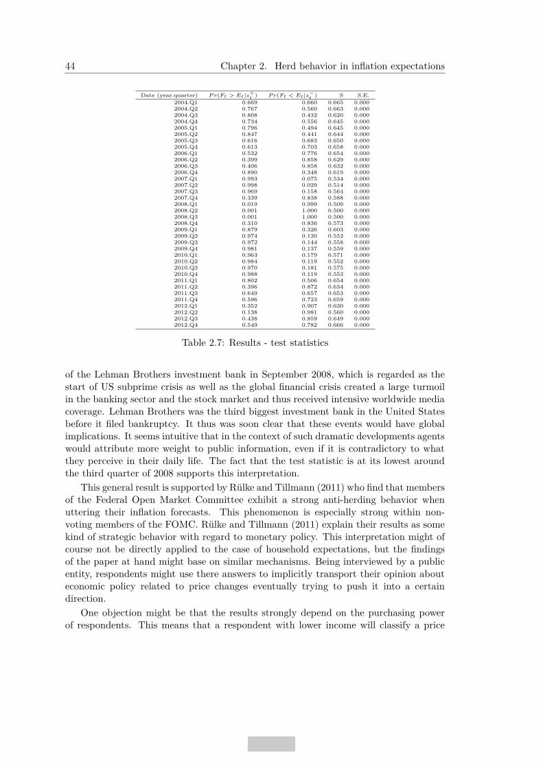
44 Chapter 2. Herd behavior in inflation expectations
Date (year.quarter) P r(Ft > Et|z+
t) P r(Ft < Et|z−
t) S S.E.
2004.Q1 0.669 0.660 0.665 0.0002004.Q2 0.767 0.560 0.663 0.0002004.Q3 0.808 0.432 0.620 0.0002004.Q4 0.734 0.556 0.645 0.0002005.Q1 0.796 0.494 0.645 0.0002005.Q2 0.847 0.441 0.644 0.0002005.Q3 0.616 0.683 0.650 0.0002005.Q4 0.613 0.703 0.658 0.0002006.Q1 0.532 0.776 0.654 0.0002006.Q2 0.399 0.858 0.629 0.0002006.Q3 0.406 0.858 0.632 0.0002006.Q4 0.890 0.348 0.619 0.0002007.Q1 0.993 0.075 0.534 0.0002007.Q2 0.998 0.029 0.514 0.0002007.Q3 0.969 0.158 0.564 0.0002007.Q4 0.339 0.838 0.588 0.0002008.Q1 0.019 0.999 0.509 0.0002008.Q2 0.001 1.000 0.500 0.0002008.Q3 0.001 1.000 0.500 0.0002008.Q4 0.310 0.836 0.573 0.0002009.Q1 0.879 0.326 0.603 0.0002009.Q2 0.974 0.130 0.552 0.0002009.Q3 0.972 0.144 0.558 0.0002009.Q4 0.981 0.137 0.559 0.0002010.Q1 0.963 0.179 0.571 0.0002010.Q2 0.984 0.119 0.552 0.0002010.Q3 0.970 0.181 0.575 0.0002010.Q4 0.988 0.119 0.553 0.0002011.Q1 0.802 0.506 0.654 0.0002011.Q2 0.396 0.872 0.634 0.0002011.Q3 0.649 0.657 0.653 0.0002011.Q4 0.596 0.723 0.659 0.0002012.Q1 0.352 0.907 0.630 0.0002012.Q2 0.138 0.981 0.560 0.0002012.Q3 0.438 0.859 0.649 0.0002012.Q4 0.549 0.782 0.666 0.000
Table 2.7: Results - test statistics
of the Lehman Brothers investment bank in September 2008, which is regarded as thestart of US subprime crisis as well as the global financial crisis created a large turmoilin the banking sector and the stock market and thus received intensive worldwide mediacoverage. Lehman Brothers was the third biggest investment bank in the United Statesbefore it filed bankruptcy. It thus was soon clear that these events would have globalimplications. It seems intuitive that in the context of such dramatic developments agentswould attribute more weight to public information, even if it is contradictory to whatthey perceive in their daily life. The fact that the test statistic is at its lowest aroundthe third quarter of 2008 supports this interpretation.
This general result is supported by Rülke and Tillmann (2011) who find that membersof the Federal Open Market Committee exhibit a strong anti-herding behavior whenuttering their inflation forecasts. This phenomenon is especially strong within non-voting members of the FOMC. Rülke and Tillmann (2011) explain their results as somekind of strategic behavior with regard to monetary policy. This interpretation might ofcourse not be directly applied to the case of household expectations, but the findingsof the paper at hand might base on similar mechanisms. Being interviewed by a publicentity, respondents might use there answers to implicitly transport their opinion abouteconomic policy related to price changes eventually trying to push it into a certaindirection.
One objection might be that the results strongly depend on the purchasing powerof respondents. This means that a respondent with lower income will classify a price

2.9. Conclusion 45
2004 Q
12004 Q
22004 Q
32004 Q
42005 Q
12005 Q
22005 Q
32005 Q
42006 Q
12006 Q
22006 Q
32006 Q
42007 Q
12007 Q
22007 Q
32007 Q
42008 Q
12008 Q
22008 Q
32008 Q
42009 Q
12009 Q
22009 Q
32009 Q
42010 Q
12010 Q
22010 Q
32010 Q
42011 Q
12011 Q
22011 Q
32011 Q
42012 Q
12012 Q
22012 Q
32012 Q
4
0.0
0.2
0.4
0.6
0.8
1.0
undershootingovershooting
Figure 2.9: Quarterly Herding Test Statistic - Jan 2004 to Dec 2012 (5% confidenceinterval)
change, be it perceived or expected, of let’s say 1.7 % per annum (the mean of inflationrate in the last twenty years in France) differently on a discrete scale with five categoriesthan a respondent with a higher income. Separating individuals into groups by clusteringmethods as the self-organizing Kohonen map would thus lead to a result in which infla-tion expectations strongly relate to personal experiences and information, appearing asanti-herding in the results above. This was however controlled for by, first, including thesociodemographic information into the fixed effects to distill the cohort/period-level per-ceptions and expectations, second, in contrast to other works using pseudo panelization,the data was not aggregated on a cohort level. This means the cohort/period-level ex-pectation and perception estimates are based on the sociodemographic variation withineach cohort. The frequently cited notion of heterogenous expectations can however notbe rejected.
A caveat for the article at hand and the results presented above lies in the data

46 Chapter 2. Herd behavior in inflation expectations
however. Bernardt et al. (2006) have, as pointed out above, designed the here appliednon-parametric test for herding to test the forecasting behavior of professional analysts.This kind of data has the following advantages: first it has a real panel structure overseveral years, second the exact point of time is known when each analyst publishedhis/her forecast, thus the sequence of forecasts is known. This is unfortunately not thecase in the French household survey data where only the month in which the surveytook place is known. Therefore a compromise had to be found, namely to apply thetest statistic quarterly, using the mean of all prior forecasts within this month as theconsensus and comparing it with the cohort-level expectations and the target inflationrate from one year ahead. This implies that a possible adjustment to a consensus, ifit takes place, could only be measured once a month and thus three times a quarter.One cannot completely exclude the possibility of different results if this information isavailable. To further investigate expectation formation with regard to inflation in thecontext of group or herd behavior, and therefore the timing of expectation formation,it would be desirable to include this information into the data sets of household sur-veys within the harmonized European household/consumer survey program or to startrecording/publishing this information when interviews are conducted.
Given the results outlined above, it would be very interesting to verify the findingsespecially with regard to the phase around the beginning of the financial crisis withother, possibly quantitative, survey questions. The University of Michigan Consumersurvey used in Chapters 3 and 4 for example contains a question which asks for quantita-tive inflation expectations. Considering the interpretation from above, namely that theanti-herding behavior with regard to inflation expectations found in this study mightbe due to agents’ heterogenous consumption behavior, it would however be probablymore interesting to repeat the herding test for variables which are more general, likegdp growth or unemployment. With quantitative data like this it would be for examplepossible to apply, knowing the distributional properties of the expectation values, sim-ulation techniques to gain better understanding of what drives consumers expectationformation process.
Acknowledgements
I would like to thank François Gardes and Christophe Starzec for their helpful com-ments, as well as my discussants at the conference of the Société canadienne de scienceéconomique 2013 (Quebec Ville, Canada) and at the Journées de Microéconomie Ap-pliqué 2013 (Nice, France).

2.A. Data References 47
2.A Data References
• Enquête de conjoncture auprès des ménages (ECAMME) - 2004 - (2004) [fichierélectronique], INSEE
• Enquête de conjoncture auprès des ménages (ECAMME) - 2005 - (2005) [fichierélectronique], INSEE
• Enquête de conjoncture auprès des ménages (ECAMME) - 2006 - (2006) [fichierélectronique], INSEE
• Enquête de conjoncture auprès des ménages (ECAMME) - 2007 - (2007) [fichierélectronique], INSEE
• Enquête de conjoncture auprès des ménages (ECAMME) - 2008 - (2008) [fichierélectronique], INSEE
• Enquête de conjoncture auprès des ménages (ECAMME) - 2009 - (2009) [fichierélectronique], INSEE
• Enquête de conjoncture auprès des ménages (ECAMME) - 2010 - (2010) [fichierélectronique], INSEE
• Enquête de conjoncture auprès des ménages (ECAMME) - 2011 - (2011) [fichierélectronique], INSEE
• Enquête de conjoncture auprès des ménages (ECAMME) - 2012 - (2012) [fichierélectronique], INSEE

48 Chapter 2. Herd behavior in inflation expectations
2.B Variance of the Test statistics
The following sections contain the procedure to compute the variance along Bernardtet al. (2006). If the realized variable πt+1 in period t + 1 in relation to the agents jposterior (the median of j’s posterior distribution over the realized variable) is given by,
πt+1 = πej,t,t+1 + �j,t+1 (2.29)
where �j,t+1 ∼ G(.) and �t+1 is independent and identically distributed over the period ofmeasurement for the forecasted variable and G(0) ≡ 0.5 and if the forecast is unbiased, itholds that πe
j,t,t+1 = πej,t,t+1, and the overshooting/undershooting indicator is distributed
binomially as,�
t
δ+t ∼ B(
�
t
γ+t , G(0))
�
t
δ−t ∼ B(
�
t
γ−t , 1 − G(0)) (2.30)
This means the test statistic S(z−t , z+
t ) is asymptotically normal distributed as
S ∼ N (0.5,116
�
1�
t γ+t
+1
�
t γ−t
�
) (2.31)
since the mean of S(z−t , z+
t ) is
12
�
P (πej,t,t+1 > πt+1) + P (πe
j,t,t+1 < πt+1)�
= 0.5[(1 − G(0)) + G(0)] = 0.5 (2.32)
and Variance corresponds to
V ar(S(z−t , z+
t )) = V ar(�
t δ+t
�
t γ+t
) + V ar(�
t δ−t
�
t γ−t
)
=1
4(�
t γ+t )2
V ar(�
t
δ+t ) +
14(
�
t γ−t )2
V ar(�
t
δ−t )
=1
4(�
t γ+t )2
G(0)(1 − G(0))(�
t
γ+t ) +
14(
�
t γ−t )2
G(0)(1 − G(0))(�
t
γ−t )
=G(0)(1 − G(0))
4
�
1�
t γ+t
+1
�
t γ−t
�
(2.33)
Accordingly in the case of a commonly unforecasted shock to the forecasted variable,ωt+1
12,�
t δ+t ∼ B(
�
t γ+t , G(−ωt)) and
�
t δ−t ∼ B(
�
t γ−t , 1 − G(−ω)), which however
leaves the mean, given the forecast is unbiased πej,t,t+1 = πe
j,t,t+1) of S(.),
12
�
P (πej,t,t+1 > πt+1) + P (πe
j,t,t+1 < πt+1)�
=12
�
P (πej,t,t+1 > πe
j,t,t+1 + ωt+1 + �j,t+1) + P (πej,t,t+1 < πe
j,t,t+1 + ωt+1 + �j,t+1)�
12thus with commonly unforecasted shock ωt+1, πt+1 = πej,t,t+1 + ωt+1 + �j,t+1

2.B. Variance of the Test statistics 49
=12
[P (�j,t+1 < −ωt+1) + P (�j,t+1 > −ωt+1)]
0.5[G(−ωt+1) + (1 − G(−ωt+1))] = 0.5
unaltered. The variance on the other hand is,
G(−ωt+1)(1 − G(−ωt+1))4
�
1�
t γ+t
+1
�
t γ−t
�
≤116
�
1�
t γ+t
+1
�
t γ−t
�
Therefore the variance is at a maximum if ω = 0 as G(−ωt+1)(1−G(−ωt+1)) ≤ G(0)(1−G(0)) = 1
2 , which means that cross-sectional correlation reduces the variance of the teststatistic. The same argumentation can also be used to show that the test statistics isrobust to the other two problems addressed above: a bias caused by optimism/pessimism,as well as measurement errors (Bernardt et al., 2006, pp. 664).

50 Chapter 2. Herd behavior in inflation expectations
2.C Robustness
The herding test of Bernardt et al. (2006) is suited for the application to inflationexpectations insofar as it is robust to systematic biases of respondents in their percep-tions/expectations.
Commonly unforecasted shocks With regard to inflation this could for examplebe a generally unanticipated rise of commodity (oil) prices due to the outbreak of anarmed conflict which would eventually lead to a shortage of supply. In this case a generalshortfall of forecasts with regard to the realized inflation, leading to the estimation ofthe conditional probability P (πt+1 < πe
t,t+1|πet,t+1 < πe
t,t+1, πet,t+1 �= πt+1) > 1
2 , andthus to the wrong conclusion that a herding-like bias was a reason for that. Consider acommonly unforecasted shock to the forecasted variable (here inflation) ωt+1 > 0, be �t+1
the idiosyncratic shock to inflation and G its cumulative distribution function. Despitea forecast is unbiased, πe
t,t+1 = πet,t+1, this would lead unconditionally to the conclusion
of herding, P (πt+1 < πet,t+1|πe
t,t+1 < πet,t+1, πe
t,t+1 �= πt+1) < 12 , since P (πe
t,t+1 + ωt+1 +�t+1 < πe
t,t+1) = P (πet,t+1 + ωt+1 + �t+1 < πe
t,t+1) = P (�t+1 < ωt+1) = G(−ωt+1) < 12 .
This is also true the other way around: with πet,t+1 = πe
t,t+1, P (πet,t+1 + ωt+1 + �t+1 >
πet,t+1) = P (πe
t,t+1 + ωt+1 + �t+1 > πet,t+1) = P (�t+1 > −ωt+1) = 1 − G(−ωt+1) > 1
2 ,which implies P (πt+1 < πe
t,t+1|πet,t+1 < πe
t,t+1, πet,t+1 �= πt+1) > 1
2 . A simple and effectivesolution, as pointed out by Bernardt et al. (2006), could be to use the average, asωt can be assumed to have offsetting effects. Under the assumption of unbiasednessπe
t,t+1 = πet,t+1, the test statistic, despite of the commonly unforecasted shock, would
still yield 0.5, as 0.5[G(−ωt+1) + (1 − G(−ωt+1))] = 12 .
Optimism/Pessimism The same would be true if a certain degree of optimism orpessimism distorts the forecasts. The phenomenon discussed by Bernardt et al. (2006)is that forecasts further in the past tend to be more optimistic, while forecasts nearer tothe disclosure of the realized value, as more information becomes available, tend to bemore pessimistic. Such an effect can be modeled by introducing a bias αt which changesover time. For example one can assume that t days before the disclosure of the realizedvalue an agent forecasts the α percentile of the forecasted value. The result could bea false conclusion with regard to the presence of herding as in the case of commonlyunforecasted earning shocks. Analogously to the latter case, this problem can alsobe addressed by taking averages, since 1
2P (πt+1 < πet,t+1|πe
t,t+1 < πt+1) + 12P (πt+1 >
πet,t+1|πe
t,t+1 > πt+1) = 12 [αt + (1 − αt)] = 1
2 rendering the conclusion if herding waspresent or not, unaltered.
Measurement errors The problem of measurement errors might become relevant, asthe value targeted by the agent in his forecast and its measurement differ (a differentperception of price changes due to different consumption behavior). As mentioned abovean individual might base its estimation of price changes on a mix of products, which isdifferent compared to the basket of goods used by the statistical office in the calculation

2.C. Robustness 51
of the official rate of inflation for a certain period of time: The agent targets πt+1 withπe
t,t+1 = πet,t+1 while the realized value πt+1 is measured as πt+1 + λt+1. Similarly, as
12P (πt+1 < πe
t,t+1|πet,t+1 < πe
t,t+1) + 12P (πt+1 > πe
t,t+1|πet,t+1 > πe
t,t+1) = 12 [G(λt+1) + (1 −
G(λt+1))] = 12 , this effect can be offset by using the average.
All the above discussed issues are also controlled for in the modification of the non-parametric test used in this article, as computing the conditional probabilities directlyfrom the estimated posterior distributions is equivalent to the averaging applied in theoriginal test proposed by Bernardt et al. (2006).

52 Chapter 2. Herd behavior in inflation expectations
2.D Variables - coding
variable type question code descriptionage numeric age - -childs numeric number of children - -citysize ordered
var.0 rural
1 less 5000 inhabitants2 between 5,000 and 9,9993 between 10,000 and
19,9994 between 20,000 and
49,9995 between 50,000 and
99,9996 between 100,000 and
199,9997 between 200,000 and
1,999,9998 Paris metropolitan re-
gioneduc ordered
var.education 1 primary education or
less2 secondary education3 post secondary educa-
tion4 tertiary education
econ_per orderedvar.
The general economicsituation in France inthe last 12 months
1 significantly worsened
2 slightly worsened3 stayed the same4 improved a bit5 significantly improved
econ_exp orderedvar.
The general economicsituation in France inthe next 12 months
1 will worsen significantly
2 will slightly worsen3 will stay the same4 will improve a bit5 will improve signifi-
cantly

2.D. Variables - coding 53
finan categoricalvar.
What descibes best thefinancial situation ofyour household
1 enough income to save asufficient amount
2 enough income to save abit
3 sufficient income tocover expenses
4 have to use reserves tocover expenses
5 coverage of expensesonly possible with bor-rowing
fracwork numeric fraction of persons inthe household with ajob
- -
price_per orderedvar.
Do you thin that pricesin the last 12 monthshave
1 decreased
2 stagnated3 increased moderately4 increased strongly
price_exp In comparison with thelast 12 months how doyou think the evolutionof prices will be in thenext 12 months
1 prices will go down
2 prices will stay the same3 prices will increase with
a smaller rate4 prices will increase with
the same rate5 prices will increase with
a faster rateregion categorical
var.region of residence 11 ÃŐle-de-France
21 Champagne-Ardenne22 Picardie23 Haute-Normandie24 Centre25 Basse-Normandie26 Bourgogne31 Nord-Pas-de-Calais

54 Chapter 2. Herd behavior in inflation expectations
41 Lorraine42 Alsace43 Franche-Comté52 Pays de Loire53 Bretagne54 Poitou-Charentes72 Aquitaine73 Midi-Pyrénées74 Limousin82 Rhône-Alpes83 Auvergne91 Languedoc-Roussilon93 Provence-Alpes-Côte
d’Azur94 Corse
revquart orderedvar.
income quartile 1 1st quartile
2 2nd quartile3 3rd quartile4 4th quartiles
sex categoricalvar.
1 male
2 femaleworkregimecategorical
var.1 full time
2 part time0or9
don’t know/no answer
spouse categoricalvar.
1 yes
2 nooccupation categorical
var.1 yes
2 no, unemployed3 no, retired4 no, inactive
birthyr numeric birthyear - -

2.E. Inflation perceptions and expectations for each cohort 55
2.E Inflation perceptions and expectations for each cohort
2004 2008 2012
−2
2
2004 2008 2012
−1
2004 2008 2012
−2
2
2004 2008 2012
−2
2
2004 2008 2012
−2
2
2004 2008 2012
−1
.5
2004 2008 2012
−1
2004 2008 2012
−2
2
2004 2008 2012
−2
2004 2008 2012
−2
2
2004 2008 2012
−2
2
2004 2008 2012
−1
2004 2008 2012
−1
.5
2004 2008 2012
−1
.5
2004 2008 2012
−2
2
2004 2008 2012
−2
2004 2008 2012
−1
2004 2008 2012
−1
2004 2008 2012
−1
.5
2004 2008 2012
−2
2
2004 2008 2012
−1
.5
2004 2008 2012
−1
2004 2008 2012
−1
.5
2004 2008 2012
−2
2
2004 2008 2012
−2
2
2004 2008 2012
−1
2004 2008 2012
−2
2004 2008 2012
−1
2004 2008 2012−
22004 2008 2012
−2
2004 2008 2012
−1
2004 2008 2012
−2
2
2004 2008 2012
−1
2004 2008 2012
−2
2
2004 2008 2012
−2
2
2004 2008 2012
−2
2004 2008 2012
−1
2004 2008 2012
−2
2
2004 2008 2012
−1
.0
2004 2008 2012
−2
2
2004 2008 2012
−2
2004 2008 2012
−2
2
2004 2008 2012
−1
.5
2004 2008 2012
−1
2004 2008 2012
−2
2004 2008 2012
−1
.0
2004 2008 2012
−1
.5
2004 2008 2012
−2
2004 2008 2012
−1
2004 2008 2012
−2
2004 2008 2012
−2
2
2004 2008 2012
−2
2
2004 2008 2012
−2
2004 2008 2012
−1
2004 2008 2012
−1
2004 2008 2012
−1
.5
2004 2008 2012
−2
Figure 2.10: Perceived inflation vs. actual inflation for each cohort

56 Chapter 2. Herd behavior in inflation expectations
2004 2008 2012
−2
2
2004 2008 2012
−1
2004 2008 2012
−2
2
2004 2008 2012
−2
2
2004 2008 2012
−2
2
2004 2008 2012
−1
.5
2004 2008 2012
−1
2004 2008 2012
−2
2
2004 2008 2012
−2
2004 2008 2012
−2
2
2004 2008 2012
−2
2
2004 2008 2012
−1
2004 2008 2012
−1
.5
2004 2008 2012
−1
.5
2004 2008 2012
−2
2
2004 2008 2012
−2
2004 2008 2012
−1
2004 2008 2012
−1
2004 2008 2012−
1.5
2004 2008 2012
−2
2
2004 2008 2012
−1
.5
2004 2008 2012
−1
2004 2008 2012
−1
.5
2004 2008 2012
−2
2
2004 2008 2012
−2
2
2004 2008 2012
−1
2004 2008 2012
−2
2004 2008 2012
−1
2004 2008 2012
−2
2004 2008 2012
−2
2004 2008 2012
−1
2004 2008 2012
−2
2
2004 2008 2012
−1
2004 2008 2012
−2
2
2004 2008 2012
−2
2
2004 2008 2012
−2
2004 2008 2012
−1
2004 2008 2012
−2
2
2004 2008 2012
−1
.0
2004 2008 2012
−2
2
2004 2008 2012
−2
2004 2008 2012
−2
2
2004 2008 2012
−1
.5
2004 2008 2012
−1
2004 2008 2012
−2
2004 2008 2012
−1
.0
2004 2008 2012
−1
.5
2004 2008 2012
−2
2004 2008 2012
−1
2004 2008 2012
−2
2004 2008 2012
−2
2
2004 2008 2012
−2
2
2004 2008 2012
−2
2004 2008 2012
−1
2004 2008 2012
−1
2004 2008 2012
−1
.5
2004 2008 2012
−2
Figure 2.11: Expected inflation vs. actual inflation for each cohort

Chapter 3
Decomposing the rationality biasin Expectations
3.1 Introduction
3.1.1 The Data Set: University of Michigan Consumer Survey
The University of Michigan consumer survey (MCS) is a household survey conductedby the Survey Research Center of the University of Michigan since 1966. Each monthat least 500 representative households from the United States excluding Hawaii andAlaska are selected and surveyed with regard to their perceptions and expectations oftheir personal economic well-being as well as general economic variables as the infla-tion rate, business conditions, unemployment rate, etc. Additionally to that the surveycollects a wide variety of sociodemographic information as for example the householdsize, the marital status, the household income, the age, the education and the race ofthe respondent. Table 3.1 gives an overview of the sociodemographic features of thesurvey respondents within the data set at the time the article at hand was written. Thedata set of the Michigan consumers survey available at the time this article was writtencomprises around 224,000 records collected between July 1980 and October 2014. Animportant and for research purposes very interesting feature of the Michigan consumersurvey is its panel structure. Although it is limited to only about 40% of the data set or89,000 respondents it allows the researcher a unique insight in the expectation formationprocess. In the specific context of the present article this feature of the survey data setpermits to compare the expectations of respondents with regard to specific variables andtheir perception thereof when they are surveyed again one year later.
3.1.2 Research question and methodology
The paper at hand ties up to the wide stream of empirical research on the rationalexpectations hypothesis. While the biggest part of the existing research focuses onthe hypothesis of rational expectations itself, some finding evidence for it like Thomas(1999) and Ang et al. (2007) others rejecting it as for example Mehra (2002), Roberts
57

58 Chapter 3. Decomposing the rationality bias in Expectations
income agesex race education n mean sd mean sd
male white no highschool 8469 23426 25055 54 19highschool 45461 42941 39804 45 17college 33588 72136 69737 46 15
afro-american no highschool 1270 17397 16968 53 18highschool 4274 35022 29083 40 15college 1839 59223 51972 43 14
hispanic no highschool 1043 23593 23742 43 17highschool 2443 41167 34824 37 14college 971 68648 64950 40 13
other no highschool 210 22332 26182 47 19highschool 1083 42009 40626 38 15college 1524 78196 74897 42 13
female white no highschool 10838 16299 18221 58 19highschool 59385 36191 34955 48 18college 31764 64120 60987 45 16
afro-american no highschool 2261 11521 12327 55 18highschool 6835 26511 23453 41 16college 2883 49061 40671 42 14
hispanic no highschool 1597 18634 19417 44 16highschool 3090 35376 33411 38 14college 1173 65549 61744 40 12
other no highschool 280 20692 22928 51 17highschool 1166 36225 38248 40 16college 1393 79189 73228 41 12All 224840 45814 49725 46 17
Table 3.1: University of Michigan Consumer Survey: Descriptive Statistics
(1997) or Baghestani (2009), this paper tackles this question from a somewhat differentperspective. Exploiting the panel structure of the Michigan consumer survey, the surveypopulation is split into two groups:
1. Respondents whose expectations and perceptions when asked one year later withregard to a certain variable correspond to each other. In other words these respon-dents would fulfill the basic notion of expectational rationality.
2. The rest of the survey population for which this is not the case, as they are eitherover- or understating the development of a certain variable when compared to theirperceptions of the same variable when asked again twelve months after the firstinterview. One could thus say that they were either too optimistic or pessimistic.Specifically this paper concentrates on the following questions or variables:1
General economic condition: The qualitative variables BEXP and BAGO in theMichigan consumer survey capture the respondents expectations and perceptions withregard to the general economic situation:
1In all cases non-responses were excluded.

3.1. Introduction 59
BEXP : “[...] do you expect that in the country as a whole business conditions will bebetter, or worse than they are at present, or just about the same?”
1. Worse a year from now
2. About the same
3. Better a year from now
BAGO: “Would you say that at the present time business conditions are better or worsethan they were a year ago?”
1. Worse now
2. About the same
3. Better now
Personal Finances: With the variables PEXP and PAGO the survey evaluates theexpectations and perceptions of respondents with regard to their personal financial sit-uation:
PEXP : “Now looking ahead – do you think that a year from now you will be better off
financially, or worse off, or just about the same as now?”
1. Will be worse off
2. Same
3. Will be better off
PAGO: “[...]Would you say that you are better off or worse off financially than youwere a year ago?”
1. Worse now
2. Same
3. Better now
Consumer Prices: The evolution of consumer prices are covered by two variables inthe survey, which are however only forward looking. PX1Q1, in the remainder of thetext coded as CPEXP _CAT , is qualitative, while P X1Q2 to which I will further referas CPEXP_PER asks for a specific quantitative value:

60 Chapter 3. Decomposing the rationality bias in Expectations
CPEXP_CAT : “[...]During the next 12 months, do you think that prices in generalwill go up, or go down, or stay where they are now?”
1. Go down
2. Same
3. Go up (at same rate or more)
In the Michigan consumer survey CPEXP_CAT is coded in four levels, this means itdifferentiates between “Go up (at the same rate)” and “Go up”. For reasons of com-parability these two categories however had that to be merged in the context of thiswork.
CPEXP_P ER: “By about what percent do you expect prices to go (up/down) on theaverage, during the next 12 months?”
Both of the questions with regard to the consumer prices are unfortunately missinga backward looking (perception) question. This problem could be circumvented in thecase of the quantitative question by using the actual inflation rate in the respectiveperiod. This is however not ideal. The perception of price evolution depends on theindividual consumption behavior and is thus highly heterogeneous 2. To take this intoaccount I am using a method suggested by Lahiri and Zhao (2015) to quantify qualitativesurvey expectations. The approach using an hierarchical ordered probit model allows toestimate time varying as well as cross-section specific threshold values which permit toconvert the true inflation rate into a cross-section specific ordered variable with threecategories. This will in turn serve as the perception variable CPPER_CAT which canbe compared to the qualitative expectation variable CPEXP_CAT . Thereby one canevaluate the expectational rationality/optimism/pessimism of an individual with regardto inflation as if both a forward looking (expectation) as well a backward looking (per-ception) variable would be available. The same method will be applied to expectationsconcerning unemployment where again only a forward looking question is available inthe Michigan consumer survey:
Unemployment: The qualitative variable UNEMP , in the remainder of the arti-cle referred to as UEEXP , captures the respondents expectations with regard to theevolution of unemployment in the 12 months ahead.
UEEXP : “How about people out of work during the coming 12 months – do you thinkthat there will be more unemployment than now, about the same, or less?”
1. Less unemployment
2. About the same2This is for example the result of Chapter 2

3.2. Decomposition Methodology 61
3. More unemployment
As mentioned above this variable also has to be quantified in order to obtain individualspecific qualitative perception information (UEPER). Once all the expectation as wellas a perception data is available, a non-linear extension of the detailed Oaxaca-Blinderdecomposition is used to investigate the differences between “rational” respondents onthe one hand and optimistic/pessimistic respondents on the other hand. In the case ofthe quantitative price expectation data in the form of the variable CPEXP_PER thestandard linear version of the Oaxaca-Blinder decomposition is used as a control.
Section 3.2 is devoted to a detailed outline of the decomposition method. In Section3.3 the HOPIT-method to quantify qualitative survey expectations is presented. It willfurther on comprise a more detailed description of how these method is used to obtaincross-section specific qualitative perception information via the estimated thresholds.Section 3.3.4 finally discusses the grouping of the survey population into rational andoptimistic/pessimistic individuals respectively and Section 3.4 presents the results of thedecomposition procedure.
3.2 Decomposition Methodology
3.2.1 Basic two-fold decomposition
The decomposition method used in this paper is an extension of the original Blinder-Oaxaca approach (Blinder, 1973; Oaxaca, 1973). Let N and K be the numbers ofobservations and parameters respectively, then Y is the N × 1 vector representing theexplained variable, X is the N × K data matrix and β is the K × 1 parameter vector.It is assumed that a function F (·), maps a linear combination of X (Xβ) to Y (Powerset al., 2011, p. 558):
Y = F (Xβ) (3.1)
The properties of F (·) depend on the respective estimation technique which in the con-text of this paper are ordinary least squares and ordered probit and will be discussedlater on. The goal in any case is to decompose the mean difference between two groupsA and B (YA − YB) into a data related effect (E) on the one hand and a coefficientrelated effect (C) on the other hand:
D = YA − YB = F (XAβA) − F (XBβB) (3.2)
=�
F (XAβA) − F (XBβA)�
� �� �
E
+�
F (XBβA) − F (XBβB)�
� �� �
C
(3.3)
The notation YB = F (XAβA) and YB = F (XBβB) refers to the mean outcomes of groupsA and B respectively. Equivalently F (XAβB) corresponds to the mean outcome com-puted using data from group A with coefficients from group B. The intuition behind theOaxaca-Blinder decomposition is the following: While for component E group specific

62 Chapter 3. Decomposing the rationality bias in Expectations
subsets of the data set are used but the same coefficients, in component C the differenceis computed using the same data subset but group specific coefficients. Component Ethus corresponds to measuring the impact of the data on the difference in outcomes as-suming that the relationship (the coefficients) between data and the outcome is invariantwith respect to the different groups. For the C component this is other way around:Using the same subset of the data but group specific coefficients allows to isolate thedifference in outcomes which are due to a difference in coefficients and thus the wayhow the data relates to the outcomes. The idea behind this sort of decomposition wasinitially to investigate to which extent the difference between wages of men and womenis related to discrimination. E therefore comprises the part of the wage gap which isexplainable by the data as for example by differences of education, work experience etc.,while C captures effects which are not explainable by the data and given the model iswell calibrated might be due to discrimination. If the estimation for example only con-tains a one explanatory variable referring to the years of schooling and A corresponds tothe male and B to the female subgroup a positive C component indicates that femalesgenerate a lower marginal gain in terms of salary for one additional year of schoolingthan their male counterparts. In other words women are rewarded to a lesser extent formore education. This means discrimination can be assumed.
A decomposition of this sort is of course sensitive to the choice of the reference group,this means to stick to the above mentioned example of the wage difference betweenmen and women on the definition of the wage which one regards as non-discriminatory.The non-discriminatory wage is not necessarily the higher one. One could for exampleassume that one part of the wage difference is due to the positive discrimination of onegroup, which means that the true non-discriminatory wage might lie between the wagerate of group A and group B. In equation (3.3) the reference group is assumed to begroup A. This assumption can be lifted by using a different non-discriminatory vectorof coefficients βR (Jann, 2008, pp. 3).
D =�
F (XAβR) − F (XBβR)�
+�
F (XBβR) − F (XBβB)�
(3.4)
In the literature different suggestions for βR can be found. Reimers (1983) suggests touse the average between the coefficient vectors of group A and B, βR = 1/2βA + 1/2βB.Cotton (1988) proposes to weight the group specific coefficients by their respective samplesizes, βR = NA/(NA + NB) ∗ βA + NB/(NA + NB) ∗ βB. A third method to approximateβR stems from Neumark (1988) who recommends to use the coefficient vector from apooled regression with group A and B.
3.2.2 Detailed Decomposition
Expression (3.4) can be further decomposed to the contribution of each parameter, thusthe weight of each parameter within both components, namely W i
∆X as far as the en-dowment effects (E) are concerned and W i
∆β for the coefficient effects (C):
D =K�
i=1
W i∆X
�
F (XAβR) − F (XBβR)�
+K�
i=1
W i∆β
�
F (XBβR) − F (XBβB)�
(3.5)

3.2. Decomposition Methodology 63
Following Yun (2004) mean characteristics are used in order to rewrite (3.4):
D =�
F (XAβR) − F (XBβR)�
+�
F (XBβR) − F (XBβB)�
+ RM (3.6)
where
RM =�
F (XAβR) − F (XBβR)�
+�
F (XBβR) − F (XBβB)�
−�
F (XAβR) − F (XBβR)�
−�
F (XBβR) − F (XBβB)�
Then the C and the E components are linearized around XAβR and XAβB by a firstorder Taylor expansions respectively.
D =δF (XAβR)δ(XAβR)
(XAβR − XBβR) +δF (XBβB)δ(XBβB)
(XBβR − XBβB)) + RM + RT
= (XA − XB)βRf(XAβR) + XB(βR − βB)f(XBβB) + RM + RT (3.7)
where
RT =�
F (XAβR) − F (XBβR)�
+�
F (XBβR) − F (XBβB)�
− (XA − XB)βRf(XAβR) + XB(βR − βB)f(XBβB)
Using (3.7) one can express the weights W i∆X and W i
∆β respectively.
W i∆X =
(X iA − X i
B)βiRf(XAβR)
(XA − XB)βRf(XAβR)=
(X iA − X i
B)βiR
(XA − XB)βR
(3.8)
W i∆β =
XiB(βi
R − βiB)f(XBβB)
XB(βR − βB)f(XBβB)=
XiB(βi
R − βiB)
XB(βR − βB)(3.9)
The weights (3.8) and (3.9) obviously have to sum up to one:�K
i=1 W i∆X = 1 and
�Ki=1 W i
∆β = 1
3.2.3 Extending the decomposition method to non-linear models
As far as linear models are concerned the mapping F (·) from X to Y is simply Xβ
and thus Y = F (Xβ) = Xβ. In an ordered probit/logit and thus non-linear frameworkwhich shall be used complementary in the article at hand this is not the case. Here thedependent variable is censored and thus only available in the form of a discrete variablewith finite, ordered response categories.
Y =
1 if Y ∗ ≤ µ1,
2 if µ1 < Y ∗ ≤ µ2,
3 if µ3 < Y ∗ ≤ µ4
...
J − 1 if µJ−1 < Y ∗ ≤ µJ−2
J if µJ−1 < Y ∗.

64 Chapter 3. Decomposing the rationality bias in Expectations
The latent variable Y ∗ is a continuous though unobserved version of the ordinal variableY . Threshold points µi with i = 1, . . . , J − 1 which are estimated within the maximumlikelihood estimation of the ordered probit model define the intervals of the latent vari-able Y ∗ which correspond to the J ordered categories. Making use of the ordered probitassumption that Y ∗ = Xβ + � with � ∼ N (0, 1) once can write down the probability foreach category:
P (Y = 1|X) = P (Y ∗ ≤ µ1|X) = P (Xβ + � ≤ µ1|X) = F (µ1 − Xβ|X)
P (Y = 2|X) = P (µ1 < Y ∗ ≤ µ2|X) = F (µ2 − Xβ|X) − F (µ1 − Xβ|X)
P (Y = 3|X) = P (µ2 < Y ∗ ≤ µ3|X) = F (µ3 − Xβ|X) − F (µ2 − Xβ|X)...
P (Y = J |X) = P (Y ∗ > µJ) = 1 − F (µJ − Xβ)
In the ordered probit case F (·) corresponds to the cumulative distribution function of thestandard normal distribution Φ(·). Using the cumulative logistic distribution functionΛ(·) would correspond to an ordered logit model. Based upon this and following Bauerand Sinning (2008) one can write down an equation for the conditional expectations ofY to which the decomposition techniques outlined in subsection 3.2.1 and 3.2.2 can beapplied.
Eβg(Yig|Xig) =
J�
j=1
j · P (Yig = j|Xig)
= 1 · [F (µ1g − Xigβg)]
+ 2 · [F (µ2g − Xigβg) − F (µ1 − Xigβg)]
+ 3 · [F (µ3g − Xigβg) − F (µ2 − Xigβg)]...
+ J · [1 − F (µJg − Xigβg)] (3.10)
Here g ∈ {A, B} again denotes the reference group to which individual i belongs. Fol-lowing Bauer and Sinning (2008) one can rewrite equation (3.10) to its sample version:
S(βg, µjg, Xig) =1N
N�
i=1
J�
j=1
j · P (Yig = j|βg, µjg, Xig)
=1N
N�
i=1
�
1 · [F (µ1g − Xigβg)]
+ 2 · [F (µ2g − Xigβg) − F (µ1 − Xigβg)]
+ 3 · [F (µ3g − Xigβg) − F (µ2 − Xigβg)]...

3.2. Decomposition Methodology 65
+ J · [1 − F (µJg − Xigβg)]�
(3.11)
Corresponding to equation (3.4) the decomposition in the context of ordinal models(probit or logit; depending on the choice of the link function) can be written as:
D =�
S(βR, µjR, XiA) − S(βR, µjR, XiB)�
+�
S(βR, µjB, XiB) − S(βB, µjB, XiB)�
(3.12)
In contrast to Bauer and Sinning (2008) it is assumed that the choice of µ in the twocomponents of the decomposition also plays a central role. The detailed decompositioncan be conducted like in the case of the linear model along equations (3.8) and (3.9).
3.2.4 Computing the Variance of the decomposition estimates
The variances for the components of the decomposition are computed following Powerset al. (2011) along the delta method introduced by Rao (Rao, 2009, pp. 321). E canbe expressed as the weighted mean of components obtained by the detailed compositionoutlined in the last but one subsection.
E =K�
k=1
Ek =K�
k=1
W∆Xk
�
F (XAβR) − F (XBβR)�
(3.13)
Taking the partial derivatives of E with respect to all βRlresults in a gradient GE with
a dimension of 1 × K of which lth element is:
δEk
δβRl
= W∆Xk
�
δF (XAβR)δβRl
−δF (XBβR)
δβRl
�
+W∆Xk
ΔβRl
�
F (XAβR) − F (XBβR)�
(3.14)
with
W∆Xk
ΔβRl
= I(k = l)�
XAk− XBk
�
k βRk(XAk
− XBk)
�
−βRl
(XAk− XBk
)(XAl− XBl
){�
k βRk(XAk
− XBk)}2
(3.15)
Here I(·) is an indicator function and, as far as non-linear models are concerned, F (Xjβj)Xjl
with j ∈ {A, B, R}. If E = (E1, . . . , EK) is the K × 1 vector with the elements of thedetailed decomposition of E, GE is the K × K gradient matrix and ΣβR
is the variance-covariance matrix of the coefficient βR, then the K × K variance-covariance matrix ofthe detailed decomposition components of E is:
ΣE = GEΣβRG�
E (3.16)
The procedure is similar for the C component.
C =K�
k=1
Ck =K�
k=1
W∆βk
�
F (XBβR) − F (XBβB)�
(3.17)

66 Chapter 3. Decomposing the rationality bias in Expectations
Along before one can again derive the gradient vector of the partial derivatives of Ck.Now however Ck depends on βR and βB. The partial derivatives thus are found byderiving Ck with respect to βR and βB respectively:
δCk
δβRl
= W∆βkf(XBβR)XBl
+Wδβk
δβRl
�
F (XBβR) − F (XBβB)�
(3.18)
δCk
δβBl
=Wδβk
δβBl
�
F (XBβR) − F (XBβB)�
− W∆βkf(XBβB)XBl
(3.19)
with
Wδβk
δβRl
= I(k = l)�
XBk�
k XBk(βRk
− βBk)
�
−XBk
XBl(βRk
− βBk)
{�
k XBk(βRk
− βBk)}2
(3.20)
Wδβk
δβBl
=XBk
XBl(βRk
− βBk)
{�
k XBk(βRk
− βBk)}2
− I(k = l)�
XBk�
k XBk(βRk
− βBk)
�
(3.21)
Again I(·) is an indicator function. If C = (C1, . . . , CK) is the K × 1 vector with theelements of the detailed decomposition of C, GCj
are the K × K gradient matricesfor j ∈ {R, B}, ΣβR
and ΣβBrespectively are the variance-covariance matrices of the
parameters of the reference group and group B regression, then the K × K variance-covariance matrix of the detailed decomposition components of C is:
ΣC = GCAΣβR
G�CA
+ GCBΣβB
G�CB
(3.22)
The variances of the overall decomposition components E and C can be found by sum-ming up the elements of the respective variance-covariance matrices of the detailed de-compositions:
V ar(E) = e�ΣEe (3.23)
V ar(C) = e�ΣCe (3.24)
where {ei}i∈I with dimension K × 1.
3.3 Obtaining cross-section specific perception data by aHOPIT-procedure
3.3.1 The hierarchical ordered probit model
One of the greatest challenges of survey based economic research is to obtain accu-rate information about the expectations of respondents with regard to various economicvariables. A natural approach would of course be to ask individuals for their quantita-tive expectations directly as this done for example in the Michigan consumer survey bythe quantitative question about the price evolution in the next twelve months (variableCPEXP_PER; for more detailed information please refer to Section 3.1). However,

3.3. Obtaining cross-section specific perception data by a HOPIT-procedure 67
research shows that while individuals have a good feeling for the trend, they often lackan accurate notion of the magnitude. It thus is the standard today in most consumersurveys to ask for qualitative information instead. The question outlined in Section 3.1(PEXP/PAGO, BEXP/BAGO, CPEXP_CAT , UEEXP ) are just a few of vari-ous examples alone in the Michigan consumer survey. It is thus not surprising that awhole stream of literature evolved around the question how to accurately quantify thequalitative survey information.
There are two families of methods to quantify qualitative survey information: Theregression method, which was introduced by Anderson (1952) and advanced by Pesaran(1985)3 on the one hand, and the probabilistic approach by Theil (1952) and Carlsonand Parkin (1975) often denoted simply as the Carlson-Parkin approach in the literatureon the other hand. The method applied here belongs to the latter category. In its basethe Carlson-Parkin approach hinges on computing theoretical cutoff-points between theordered categories in an assumed probability distribution using the share of respondentsin the individual categories. The thereby estimated results are just identified up to ascale parameter and have to be calibrated subsequently. For the calibration in its mostbasic form normally the last observed value from the variable in question is used, asthis is assumed to be the value which the respondents had in mind when answering thequestion about the expected future evolution of the same variable. This approach hasfour major drawbacks:
1. the cutoff-points (or thresholds) between the three categories (thus between cat-egory 1 and 2 as well as between category 2 and 3 in the three category case ofthe Michigan consumer survey 4) are by design symmetric around zero (the inter-val between the two thresholds is often referred to as the “indifference limens”,thus the interval in which respondents would notice no change in the variable inquestion and thus choose category 2)
2. the thresholds are constant over time
3. shortcoming 2. could be circumvented by estimating the thresholds period byperiod, this however often leads to the problem of zero-responses: the standardCarlson-Parkin approach cannot be estimated if there are no responses in one ofthe categories
4. the standard Carlson-Parkin approach doesn’t allow to control for heterogeneityamong survey participants
5. the standard calibration technique implicitly assumes the unbiasedness of percep-tions/expectations and is thus unsuitable to test the rational expectation hypoth-esis
3see also Pesaran (1987) and Pesaran and Weale (2006b)4Berk (1999) proposes a technique for five answering categories, it however has the same shortcomings
as the standard Carlson-Parkin approach with three categories.

68 Chapter 3. Decomposing the rationality bias in Expectations
Kaiser and Spitz (2002) show that the Carlson-Parkin method can be generalized in anordered probit model (or depending on the distributional assumptions also in an orderedlogit model). This allows to solve the problems listed above under points 1. to 4., ithowever doesn’t allow to estimate cross-section specific thresholds. The heterogeneitythereof is only controlled for implicitly by including individual specific variables in theestimation of the ordered probit model. Estimating the ordered probit model with anintercept only is exactly equivalent to the Carlson-Parkin approach (the results are likein the case of the standard Carlson-Parkin approach only identified up to scale and thushave to be calibrated afterwards).
In the context of the present article I am adopting an approach proposed by Lahiriand Zhao (2015) who use an hierarchical ordered probit model (HOPIT) to quantify thequalitative survey expectations5. It overcomes the problems outlined above and allowsto estimate cross section specific threshold values. As in the paper by Lahiri and Zhao(2015) a time varying parameter model (estimated in a state space framework) is utilizedto calibrate the results. This permits to circumnavigate the unbiasedness assumption.
The HOPIT model, also denoted as generalized ordered choice model, was introducedby Eluru et al. (2008) and advanced by Greene and Hensher (2010). It belongs to thefamily of probabilistic methods and is estimated by maximizing the following likelihoodfunction:
LHOP IT =T�
t=1
Nt�
t=1
�
I{yit = 1} × ln�
φ
�δit,1 − y∗
t
σit
���
+T�
t=1
Nt�
t=1
�
I{yit = 2} × ln�
φ
�δit,2 − y∗
t
σit
�
− φ
�δit,1 − y∗
t
σit
���
+T�
t=1
Nt�
t=1
�
I{yit = 3} × ln�
1 − φ
�δit,2 − y∗
t
σit
���
(3.25)
The difference to the standard ordered probit model is that the latent variable y∗t , the
lower δit,1, the upper threshold δit,2 and the variance σit are specified on a cross sectionlevel by the following equations:
y∗it = yt + �it (3.26)
δit,1 = γ0 + exp(Wi,t−hβ1w) (3.27)
δit,2 = δit,1 + exp(Wi,t−hβ2w) (3.28)
σit = exp(Zi,t−hβz) (3.29)
Wi,t−h ∈ Xi,t−h and Zi,t−h ∈ Xi,t−h represent the model matrices formed from indepen-dent variables Xi,t−h in the survey. Both matrices are allowed to have overlappings withregard to the variables they contain. y∗
it is the qualitative responses by individual i atperiod t. h corresponds to the forecast horizon, which in the context of this article istwelve months. The parameters γ0, β1w, β2w and βz as well as the thresholds in the
5I am grateful to Yongchen Zhao for his helpful comments.

3.3. Obtaining cross-section specific perception data by a HOPIT-procedure 69
linear latent equation have to be estimated. The formulation of the threshold equationswith exponential functions and δit,1 in equation (3.27) ensures that the thresholds areordered. The inclusion of γ0 at the same time allows the thresholds to be negative.To quantify the variable CPEXP_CAT the same parametrization as in the paper by(Lahiri and Zhao, 2015) is used:
• latent equation:
– dummy variables indicating the months covered by the survey since July 1980
• threshold equation(s):
– PAGO - perceptions with regard to personal finances; please refer to Section3.1
– PEXP - expectations with regard to personal finances; please refer to Section3.1
– BAGO - perceptions with regard to the general economic conditions; pleaserefer to Section 3.1
– BEXP - expectations with regard to the general economic conditions; pleaserefer to Section 3.1
– UEEXP - expectations with regard to the unemployment rate; please refer toSection 3.1
– RATEX - expectations with regard to the interest rates (categorical)
– GOVT - evaluation of perceived government performance (categorical)
– HOM - attitude towards buying real estate (categorical)
– CAR - attitude towards buying a car (categorical)
– AGE - age of the respondent (continuous)
– INCOME - income in USD of the respondent (continuous)
– SEX - gender of the variable (categorical)
– EDUC - education level of the respondent (categorical)
• variance equation:
– BAGO
– UEEXP
– RATEX
– GOVT
– AGE
– SEX
– EDUC

70 Chapter 3. Decomposing the rationality bias in Expectations
– RACE - as defined by the respondent (categorical)
For the estimation of the expectation variable with regard to the unemployment rateonly the roles of CPEXP_CAT and UEEXP were exchanged. The likelihood functionwas implemented in C++6, and augmented by an auto-differentiation algorithm (Fournieret al., 2012) to speed up convergence of the likelihood estimation. The whole procedurecomprises the estimation of in both cases 482 parameters. The parameter estimates canbe found in Appendix 3.D. In order to ensure that the same parameters have the sameeffect on the upper and lower threshold but to allow divergence if the effects are indeedsignificantly different a soft, differentiable penalty function was integrated.
As it is often the case for non-linear models of this magnitude the resulting Hessianmatrix is not invertible. A numerical trick using the the general inverse and a generalCholesky decomposition proposed by Gill and King (2004) is applied to compute thestandard errors anyway 7.
3.3.2 Calibration
As mentioned before the result y∗t obtained by the HOPIT method outlined in the
previous subsection are only identified up to scale. The results thus have to be calibrated.In order to render the results suitable for testing the rational expectation hypothesis, acalibration via a time varying parameter model with AR(1) structure as suggested by(Lahiri and Zhao, 2015) is utilized. Although this study doesn’t contain a rationality testin the normal fashion, for reasons discussed in the last subsection it seems appropriate toavoid the unbiasedness assumption. The time varying parameter model can be writtenin form of a state space model:
measurement equation: pt = βty∗t
transition equation: βt = α + γβt−1 + �t
Here pt is the reference value for the estimated variable. In the case of the estimation ofthe expected inflation rate and the expected unemployment rate these variables are thelatest observed inflation and unemployment rates respectively. The first order Markovprocess in the transition equation (the autoregressive term AR(1)) ensures a smoothevolution of states over time and thus of the relationship between the raw estimatesfrom the HOPIT model and the reference variable. The serially uncorrelated Gaussiandisturbance term � with mean zero captures transitory shocks. The final calibratedquantified estimates of the variables in questions eventually are the twelve month aheadforecasts of pt. The monthly means of the threshold variables obtained by the crosssection specific estimates δit,1 = γ0 + exp(Wi,t−hβ1w) and δit,2 = δit,1 + exp(Wi,t−hβ2w)are subsequently rescaled proportionally. The thereby calibrated, monthly threshold
6For the source code the reader is referred to Appendix 3.C.7Be H−1 the general inverse of the Hessian matrix and V = GCHOL(H−1) the Cholesky decompo-
sition thereof, then V �V is the pseudo-variance matrix which can subsequently be used to compute thestandard errors and the p-values.

3.3. Obtaining cross-section specific perception data by a HOPIT-procedure 71
0
4
8
12
1980 1985 1990 1995 2000 2005 2010 2015
infla
tio
n r
ate
− %
expected inflation
inflation
Figure 3.1: Quantification of qualitative expectations of the inflation rate with the HO-PIT method (the shaded areas in the plot correspond to the recession periods along thedefinition of the Federal Reserve Bank)
means δct,1 and δc
t,2 are then used to rescale the cross section specific estimates δit,1 andδit,2. Figure 3.1 and Figure 3.2 display the thereby estimated quantified expectations ofthe inflation and unemployment rate and compare these values to the actual measuredvariables. The grey ribbon represents in both cases the indifference limens, thus thearea between the lower and the upper threshold in which the respondent (in the theplots naturally only the means can be displayed) doesn’t notice a change and would thuschoose category two. That the line is mostly above the indifference limens indicates thatin most periods the majority of respondents chose category three.
3.3.3 Converting the realized values into individual specific perceptionestimates
Using the method outlined above the calibrated thresholds δcit,1 and δc
it,2 are now availableon an individual level for both the inflation and the unemployment rate. This informa-tion can be utilized to recode the realized values in order to obtain individual-specificperception estimates. This is done by comparing the reference variable from twelvemonths ahead pt+12 with the calibrated individual specific threshold estimates δc
it,1 andδc
it,2 . If pt+12 < δcit,1 the perception variable is coded as 1, if δc
it,1 ≤ pt+12 ≤ δcit,2 as 2
and if δcit,2 < pt+12 as 3. Thereby one obtains estimates for the variables CPPER_CAT
and UEPER.

72 Chapter 3. Decomposing the rationality bias in Expectations
0
10
20
30
1980 1985 1990 1995 2000 2005 2010 2015
un
em
plo
ym
en
t ra
te −
%
expected unemployment
unemployment
Figure 3.2: Quantification of qualitative expectations of the unemployment rate withthe HOPIT method (the shaded areas in the plot correspond to the recession periodsalong the definition of the Federal Reserve Bank)
3.3.4 Partitioning the survey population into rational and non-rationalindividuals
With individual specific estimates for the perception variables CPPER_CAT andUEPER at hand, one can now move on to evaluate the expectational rationality ofindividual survey respondents. It has to be noted that this doesn’t involve a rationalitytest of the type which standardly can be found in the literature, normally applied toaggregate data. It however allows to partition the survey population into two groups:
1. A group with individuals whose expectations correspond to their perceptions twelvemonths later.
2. A group with individuals who are either too optimistic or pessimistic in theirexpectations if one compares them with their perceived values twelve months later.
An individual is considered to have rational expectations for a specific variable if thefollowing conditions are fulfilled respectively:
BEXP − BAGO = 0
PEXP − PAGO = 0
CPEXP_CAT − CPPER_CAT = 0
BEXP − BAGO = 0
UEPER − UEEXP = 0
For the sake of comparability with the other variables the equation was reversed in thecase of unemployment. It is interesting to look at the evolution of these differences or

3.3. Obtaining cross-section specific perception data by a HOPIT-procedure 73
personal_finances
business
prices_per
prices_cat
unemployment
0.00
0.25
0.50
0.75
1.00
0.00
0.25
0.50
0.75
1.00
0.00
0.25
0.50
0.75
1.00
0.00
0.25
0.50
0.75
1.00
0.00
0.25
0.50
0.75
1.00
1980 1985 1990 1995 2000 2005 2010 2015
op
tim
ism
vs.
pe
ssim
ism
Figure 3.3: Optimism, Pessimism and Rationality over time (the shaded areas in the plotcorrespond to the recession periods along the definition of the Federal Reserve Bank)
better their respective average over time. They are displayed in Figure 3.3. Looking atFigure 3.3 there are two striking features:
1. There is a noticeable correlation between the variables and
2. the degree of overstated expectations is especially high during phases of recession,marked by the light red shade in the plots.8
It might seem counter-intuitive that an overstatement of inflation expectations is re-garded as optimistic attitude. This is however in line with economic theory and empiri-cal findings: Higher growth goes hand in hand with an upward pressure on prices. Thisrelation seems to be one which also the respondents of the Michigan consumer surveyseem to have internalized.
With these grouping variables at hand one can now proceed to investigate the dif-ferences between rational individuals on the one hand and optimistic/pessimistic indi-viduals on the other hand using the extended Oaxaca-Blinder decomposition methodsoutlined in Section 3.2. For the quantitative expectation variable CPEXP_PER andCPPER_PER the condition CPEXP_CAT − CPPER_CAT = 0 is used as a ratio-nality indicator.
8For the recession dates information from the National Bureau of Economic Research (NBER) wasused: https://research.stlouisfed.org/fred2/series/USREC

74 Chapter 3. Decomposing the rationality bias in Expectations
3.4 Results & Conlusion
The results of the Oaxaca-Blinder methods are displayed in Tables 3.2 to 3.11 in Ap-pendix 3.A of this chapter. The two result tables per variable-group corresponds tothe detailed Oaxaca-Blinder method by reference-group and the Neumark pooled re-gression method respectively. The results are evaluated and interpreted in what followsby the different components of the decomposition results: differences, endowment andcoefficients:
3.4.1 Differences
What can be observed in the upper part of the results tables in Appendix 3.A is that thegroup of non-rational respondents along the definition from the last section systemati-cally overestimates the variables in question. The difference values are with the exceptionof the decomposition with regard to the expected unemployment rate all negative. Inthe case of the unemployment rate the interpretation has to be reversed as we had previ-ously switched the rationality conditions for coherence reasons (the unemployment rateis the only variable under consideration in which a lower value corresponds to a moreoptimistic attitude; for further information the reader is referred to Section 3.3.4). Therespective result is thus not a contradiction: One could state that the rational agentis in general less optimistic /more pessimistic than the greater number of non-rationalsurvey respondents. This effect is especially pronounced when looking at the Tables 3.2and 3.3 which compare the quantitative expectation values with regard to inflation tothe realized inflation. As noted above, these values have to be interpreted with cautionas in this case no real perception values are available and thus only the realized inflationrates were used. The conclusion however stays the same. For the other variables therationality bias lies between 0.027 and 0.064.
3.4.2 Endowment effects, coefficient effects
The main result of this paper is, that the rationality bias can be significantly and to alarge extent explained by endowment effects. Sometimes the literature refers to this partas the explained part, while the coefficient effects are denoted as the unexplained part,as it cannot be explained by the explanatory variables included in the estimation. Inthe gender wage gap literature from which this method originally comes, the explainedpart is seen as the part of the difference between male and female wages which can beexplained by differences in education, work experience (due to pregnancy women oftenhave less working years) etc.. The coefficient effects are unexplained however and canthus be interpreted as due to discrimination.
In the context of this article the endowment part can be interpreted as the partof the differences between rational and non-rational agents which can be explained bythe data. The rest (the coefficient effects) must be seen as some kind of unexplainedbias which influences the expectation formation of agents. These could be for examplepersonal circumstances which can of course not be covered in full detail by a study as

3.4. Results & Conlusion 75
the Michigan consumer survey. The endowment effects reach from 16% as far as thenon-linear decomposition of consumer price expectations are concerned to up to around60% as far as business climate and unemployment rate expectations are concerned. Inall these cases the endowment effects are highly significant. More caution has to beapplied in interpreting negative signs before the endowment percentages in the non-linear decomposition of rationality biases for consumer prices and personal finances: Itsignifies some kind of potential difference between the group of rational and non-rationalagents. As mentioned before, the signs in front of the difference values9 imply that thegroup of non-rational agents in average tends to be more optimistic relative to the groupof rational-agents, this means their expectations overstate the reality as perceived twelvemonths later.
The negative sign in front of the percentages imply that this effect would be evengreater for the concerned variables if the rational agents would have the same sociodemo-graphic characteristics. Considering the notion of heterogeneity in expectations it mightnot be surprising that this effect is observable when decomposing the rationality bias forvariables as individually specific as consumer prices (the experience of prices changes ofcourse very much depends on ones consumption behavior) and personal finances. Whatall this means in detail will be seen when taking a closer look at the coefficients in theendowment effects. For the decomposition the following variables were included:
• sex - the gender of the respondent (categorical)
• white - dummy variable indicating a respondent is white
• egrade - years of education (continuous, centered)
• workingage - dummy variable indicating if a respondent is below 65 years old andcould thus be attributed to the labor force
• income - income in USD (continuous, centered)
• news1 and news2 - dummy variable indicating if the respondent has perceivedpositive or negative news with regard to the economy prior to interview
Going systematically from upside down, the following interpretation can be given for thecoefficient estimates in the detailed Oaxaca-Blinder decomposition. One has to note thatthe interpretation is given in terms of the effect on the rationality bias since this seemsmore natural, especially as the sign for the unemployment decomposition are reversedwhich could create confusion. A positive percentage next to a coefficient thus implies thatthe effect described above (the group of non-rational individuals being overly optimisticwhen compared to the group of rational agents), while a negative percentage implies aweakening effect on the rationality bias.
9They were negative for several decomposition results with the exception of unemployment, since forthe latter we swapped directions for the rationality condition; for more information please refer to thelast Subsection as well as Section 3.3.3.

76 Chapter 3. Decomposing the rationality bias in Expectations
Being male (sex1) has a positive percentage contribution for the rationality bias forall decomposition results. It thus increases the above described gap between rationaland non rational agents. The results for the variable indicating if a respondent is whiteincreases the gap for consumer prices (in the linear case), business climate and the un-employment rate. The opposite is true for personal finances and the consumer prices(non-linear case). Education increases the gap for consumer prices (linear case), con-sumer prices (non-linear case when using coefficient pooling is used: Neumark), personalfinances, business climate and the unemployment rate. The opposite is true for the othervariables. Being in the labor force, thus below age 65 (workingage1), has a wideningeffect on the gap with exceptions for the variables consumer prices (linear and non-linearwith the reference group method) and personal finances. The respondents income has areinforcing effect on the gap for all variables with the exception of consumer prices (non-linear case, reference group), business climate and unemployment. Last but not least,the perception of news (bad or good) has a very strong and significant re-enforcing effecton the rationality gap in general. This is especially true for the variables unemploymentand business climate, thus in short for variables which can only evaluated by individualsusing external information, thus news.
The unexplained effects (coefficient effects) seem to play a role, which however can-not be accurately evaluated by the data for most of the variables, i.e. they are notsatisfyingly significant in all the cases. The only decomposition results which indicate a“better” measurable contribution of unobserved effects are consumer prices (non-linearcase, reference group), personal finances and business climate. Again these results mightbe attributed to the fact that these variables can be considered as highly subjective.
3.4.3 Conclusion and Policy implications
It can be concluded that differences in rationality within the survey population comprisedin the data set of the Michigan consumer survey available at the time this study wasconducted can be to a large and significant extent explained by the sociodemographicstatus of an individual represented by gender, race, age, income, education or informationabout the individuals supplied with the survey (inter alia news consumption) in the aboveestimations. With regard to variables which are somehow outside of the daily experiencehorizon for most individuals (for example unemployment and business climate), theeffect of news perception is especially strong. The unexplained part, due to unobservedindividual effects, on the other hand can unfortunately only be quantified in a veryinaccurate manner: The tendencies however tell a similar story. The only variableswhere the unobserved effects can be measured with halfway acceptable precision arehighly subjective in character, namely consumer prices and personal finances.
Overall the findings outlined above point in a similar direction as the results ofChapter 2 where I found a significant anti-herding behavior of agents in their expectationformation with regard to inflation. This anti-herding behavior which corresponds to abias away from the consensus expectation can be interpreted as due to a differentiatedconsumption behavior among agents which is also reflected in different expectations asfar as the future evolution of prices is concerned. This, as stated above, supports the

3.4. Results & Conlusion 77
hypothesis of heterogenous expectations. The two most important points which can bedrawn from the findings in this chapter have similar implications:
1. The accuracy of expectations with regard to objectively measurable realized vari-ables highly depends on the individuals sociodemographic status or expressed dif-ferently, the difference between, along the here used definition, “rational” and“non-rational” is largely explainable by data. The notion of rationality in this con-text might thus be not appropriate as the rationality bias seems to depend mostlyon the sociodemographic background of agents.
2. For expectations with regard to variables as consumer prices or personal finances,which, as argued above, very much reflect the subjective experience horizon ofan agent this effect is weaker. In these cases one might assume that individualfactors play a role which cannot be captured by a standardized household survey.A deviation from the here used rationality condition as far as the survey questionwith regard to personal finances is concerned, could be for example due to a shockto the individual financial situation of an agent, which could impossibly have beenforeseen at the time when the first interview was conducted (in this context onmight think about costly maintenance work for housing or vehicles, or since thisstudy uses data from the United States of America, unexpected high medical bills).
Support for the hypothesis of heterogenous expectations, both empirically and experi-mentally, can be also found in the literature. Mankiw et al. (2004) find with data fromvarious sources, one of which is the Michigan Consumer survey, that there is substantialdisagreement among agents with regard to inflation expectations varying in differenteconomic situations. Branch (2004) shows, as well using inflationary expectation datafrom the Michigan Consumer Survey, that agents choose from a set of different costlypredictor functions when forming their believes with regard to inflation in the next twelvemonths. Hommes (2011) chooses a similar approach trying to fit different forecastingheuristics to data from a “Learning-to-Forecast Experiment”. It is shown that homoge-nous expectation models are, independent from the market setting, inappropriate to fitthe data gained from the experiment. Effective learning and thus convergence to therational expectation condition only occurred when using a cobweb market frameworkwith negative learning feedback similar to that used by Muth (1961) in his seminalpaper. These two papers connect to earlier contributions by for example Frankel andFroot (1987, 1990) or Taylor and Allen (1992) who show that professional forecasters em-ploy different techniques to predict future exchange rates. Capistrán and Timmermann(2009) find evidence that the degree of heterogeneity among professional forecasterswith regard to future inflation underlies a strong variation over time which magnitudedepends on the level as well as the volatility of inflation. The only study which, to theknowledge of the author, relates the notion of heterogenous expectations to the sociode-mographic background by consumers is by Pfajfar and Santoro (2009). Concentrating aswell on expectations with regard to inflation expectations, the authors find evidence thatconsumers rather concentrate on the CPI relevant for their sociodemographic subgroup

78 Chapter 3. Decomposing the rationality bias in Expectations
than on the general future inflation rate as it is surveyed by consumer surveys as theUniversity of Michigan Consumer survey.
The findings outlined above are relevant for policy makers as well as for researchers.On the one hand variables which turn out to be especially susceptible to individuallyspecific effects (as mentioned above expectations with regard to personal finances and in-flation fall in this category) are of very high relevance for policy decisions and announce-ments thereof, especially with regard to monetary policy. They are highly subjectivethus hard to assess for policymakers. More research is therefore needed to investigatethe rationality bias in these topical areas, as a one-fits all policy could have unintendedeffects for some parts of the society. For researchers the results indicate a row of otherinteresting questions: Can the focus on “rational” agents lead to better forecasts ofrealized variables, be it inflation or household consumption? What could be possiblefactors for the rationality bias which cannot be explained by the data (correspondingto th unexplained part in the results)? The next Chapter 4 tries to contribute to thisdebate by evaluating the role of social influences on the expectations formation.

3.A. Decomposition Results 79
3.A Decomposition Results
Consumer Prices (linear)
Diff. StdErr z-value Pr(>|z|) Pct. overall Pct.
Difference -0.724 100Endowment -0.145 0.193 -0.749 0.847 19.985Coefficients -0.579 26.664 -0.022 0 80.015
Endowment: detailsex1 0.078 0.008 10.013 0.994 -10.761 2.712sex2 -0.098 0.039 -2.494 0.969 13.472
white1 -0.002 0.001 -3.681 1.000 0.279 0.279egrade -0.074 0.081 -0.916 0.935 10.259 10.259
workingage1 0.005 0.010 0.471 0.992 -0.669 -0.669income -0.043 0.163 -0.263 0.870 5.915 5.915news1 0.004 0.012 0.307 0.990 -0.521 1.490news2 -0.015 0.015 -0.951 0.988 2.010
Coeffcient: detailsex1 -0.194 0.819 -0.237 0.413 26.785 45.701sex2 -0.137 1.039 -0.132 0.299 18.916
white1 -0.086 2.482 -0.034 0.013 11.807 11.807egrade -0.003 29.087 -0.0001 0 0.455 0.455
workingage1 -0.265 1.182 -0.224 0.237 36.568 36.568income 0.113 2.296 0.049 0.022 -15.638 -15.638news1 0.011 5.957 0.002 0 -1.477 1.122news2 -0.019 2.581 -0.007 0.010 2.598
Table 3.2: Linear decomposition of the expectation bias - consumer prices (referencegroup)
Diff. StdErr z-value Pr(>|z|) Pct. overall Pct.
Difference -0.724 100Endowment -0.207 0.077 -2.684 0.939 28.587Coefficients -0.517 15.049 -0.034 0 71.413
Endowment: detailsex1 0.081 0.005 17.267 0.996 -11.229 2.586sex2 -0.100 0.010 -10.302 0.992 13.816
white1 -0.002 0.0005 -3.981 1.000 0.253 0.253egrade -0.075 0.021 -3.553 0.983 10.298 10.298
workingage1 -0.006 0.009 -0.648 0.993 0.766 0.766income -0.094 0.068 -1.391 0.946 13.032 13.032news1 0.005 0.008 0.587 0.994 -0.659 1.651news2 -0.017 0.007 -2.549 0.995 2.311
Coeffcient: detailsex1 -0.182 1.408 -0.129 0.159 25.102 39.913sex2 -0.107 2.473 -0.043 0.013 14.811
white1 -0.087 5.036 -0.017 0 12.057 12.057egrade -0.013 15.639 -0.001 0 1.728 1.728
workingage1 -0.256 1.595 -0.161 0.111 35.384 35.384income 0.127 4.182 0.030 0.00003 -17.594 -17.594news1 0.015 8.956 0.002 0 -2.062 -0.075news2 -0.014 6.984 -0.002 0 1.987
Table 3.3: Linear decomposition of the expectation bias - consumer prices (Neumark)

80 Chapter 3. Decomposing the rationality bias in Expectations
Consumer Prices (non-linear)
Diff. StdErr z-value Pr(>|z|) Pct. overall Pct.
Difference -0.016 100Endowment 0.004 0.002 1.646 0.998 -24.402Coefficients -0.020 0.175 -0.117 0.861 124.402
Endowment: detailsex1 -0.0001 0.0001 -1.078 1.000 0.841 0.841
white1 0.00003 0.00003 1.021 1.000 -0.160 -0.160egrade 0.0004 0.0002 1.830 1.000 -2.549 -2.549
workingage1 0.001 0.0003 1.796 1.000 -3.456 -3.456income 0.003 0.002 1.556 0.998 -20.642 -20.642news1 -0.0002 0.0002 -1.023 1.000 1.226 1.564news2 -0.0001 0.0002 -0.287 1.000 0.338
Coeffcient: detailsex1 0.001 0.148 0.006 0.882 -5.302 -5.302
white1 0.013 0.024 0.531 0.981 -77.021 -77.021egrade 0.007 0.051 0.127 0.959 -39.622 -39.622
workingage1 -0.053 0.039 -1.383 0.969 323.899 323.899income 0.027 0.027 0.982 0.978 -163.763 -163.763news1 -0.006 0.044 -0.131 0.965 34.987 86.211news2 -0.008 0.025 -0.338 0.980 51.224
Table 3.4: Non-Linear decomposition of the expectation bias - consumer prices (referencegroup)
Diff. StdErr z-value Pr(>|z|) Pct. overall Pct.
Difference -0.014 100Endowment -0.002 0.001 -2.871 0.999 16.354Coefficients -0.012 0.149 -0.081 0.881 83.646
Endowment: detailsex1 -0.0001 0.0001 -0.804 1.000 0.468 0.468
white1 0.00001 0.00001 0.862 1.000 -0.086 -0.086egrade -0.00003 0.0001 -0.222 1.000 0.185 0.185
workingage1 -0.0003 0.0002 -1.751 1.000 2.350 2.350income -0.001 0.001 -1.603 0.999 8.317 8.317news1 -0.0003 0.0002 -1.932 1.000 2.209 5.119news2 -0.0004 0.0002 -2.632 1.000 2.910
Coeffcient: detailsex1 0.002 0.124 0.015 0.901 -12.475 -12.475
white1 0.023 0.029 0.802 0.977 -161.322 -161.322egrade 0.013 0.046 0.274 0.963 -86.935 -86.935
workingage1 -0.067 0.077 -0.862 0.938 461.668 461.668income 0.040 0.032 1.247 0.975 -273.728 -273.728news1 -0.011 0.040 -0.262 0.968 72.763 156.438news2 -0.012 0.029 -0.416 0.977 83.675
Table 3.5: Non-Linear decomposition of the expectation bias - consumer prices (Neu-mark)

3.A. Decomposition Results 81
Personal Finances (non-linear)
Diff. StdErr z-value Pr(>|z|) Pct. overall Pct.
Difference -0.025 100Endowment 0.002 0.003 0.861 0.998 -10.007Coefficients -0.027 12.497 -0.002 0 110.007
Endowment: detailsex1 -0.0005 0.0004 -1.278 1.000 1.973 1.973
white1 0.001 0.0002 2.960 1.000 -2.752 -2.752egrade -0.0003 0.0001 -2.176 1.000 1.173 1.173
workingage1 0.005 0.002 2.079 0.998 -20.926 -20.926income -0.00002 0.00005 -0.423 1.000 0.077 0.077news1 -0.0001 0.0001 -0.615 1.000 0.309 10.448news2 -0.002 0.0005 -5.373 1.000 10.139
Coeffcient: detailsex1 0.001 0.420 0.002 0.674 -3.284 -3.284
white1 -0.004 0.031 -0.118 0.975 15.031 15.031egrade -0.002 0.031 -0.066 0.976 8.138 8.138
workingage1 -0.030 0.013 -2.246 0.989 122.470 122.470income 0.00001 12.280 0 0 -0.031 -0.031news1 -0.001 0.182 -0.004 0.856 2.604 -32.318news2 0.009 0.015 0.573 0.988 -34.922
Table 3.6: Non-Linear decomposition of the expectation bias - personal finances (refer-ence group)
Diff. StdErr z-value Pr(>|z|) Pct. overall Pct.
Difference -0.026 100Endowment 0.002 0.003 0.989 0.998 -9.740Coefficients -0.028 52.698 -0.001 0 109.740
Endowment: detailsex1 -0.002 0.0004 -3.676 1.000 6.116 6.116
white1 0.001 0.0002 3.600 1.000 -3.177 -3.177egrade -0.001 0.0002 -5.825 1.000 4.903 4.903
workingage1 0.011 0.002 4.547 0.998 -42.311 -42.311income -0.00003 0.00005 -0.606 1.000 0.109 0.109news1 -0.0001 0.0001 -0.575 1.000 0.296 24.619news2 -0.006 0.001 -6.821 0.999 24.323
Coeffcient: detailsex1 0.001 1.072 0.001 0.284 -2.331 -2.331
white1 -0.003 0.066 -0.050 0.947 12.853 12.853egrade -0.002 0.058 -0.034 0.954 7.773 7.773
workingage1 -0.031 0.011 -2.759 0.991 122.278 122.278income 0 53.465 0 0 0.013 0.013news1 -0.001 0.254 -0.003 0.800 3.379 -30.846news2 0.009 0.028 0.317 0.978 -34.225
Table 3.7: Non-Linear decomposition of the expectation bias - personal finances (Neu-mark)

82 Chapter 3. Decomposing the rationality bias in Expectations
Business Climate (non-linear)
Diff. StdErr z-value Pr(>|z|) Pct. overall Pct.
Difference -0.016 100Endowment -0.010 0.0004 -27.664 1.000 61.357Coefficients -0.006 0.168 -0.037 0.867 38.643
Endowment: detailsex1 -0.001 0.001 -2.324 1.000 7.639 7.639
white1 -0.0001 0.0001 -0.384 1.000 0.347 0.347egrade -0.0003 0.0001 -2.195 1.000 1.839 1.839
workingage1 -0.001 0.001 -1.364 1.000 4.478 4.478income 0 0.00004 0.063 1.000 -0.017 -0.017news1 -0.0002 0.0001 -1.281 1.000 0.989 47.071news2 -0.007 0.001 -10.346 0.999 46.082
Coeffcient: detailsex1 0.0004 0.224 0.002 0.822 -2.581 -2.581
white1 -0.0001 0.221 -0.001 0.825 0.899 0.899egrade -0.001 0.024 -0.028 0.981 4.271 4.271
workingage1 -0.008 0.010 -0.806 0.992 50.679 50.679income -0.0002 0.134 -0.001 0.893 1.175 1.175news1 -0.001 0.050 -0.013 0.960 4.002 -15.800news2 0.003 0.011 0.284 0.991 -19.802
Table 3.8: Non-Linear decomposition of the expectation bias - business climate (referencegroup)
Diff. StdErr z-value Pr(>|z|) Pct. overall Pct.
Difference -0.016 100Endowment -0.010 0.0003 -35.256 1.000 62.487Coefficients -0.006 0.148 -0.041 0.882 37.513
Endowment: detailsex1 -0.001 0.0004 -3.846 1.000 8.768 8.768
white1 -0.0001 0.0001 -0.531 1.000 0.344 0.344egrade -0.0004 0.0001 -4.561 1.000 2.732 2.732
workingage1 -0.0002 0.0004 -0.491 1.000 1.147 1.147income 0.00001 0.00003 0.290 1.000 -0.055 -0.055news1 -0.0001 0.0001 -1.570 1.000 0.876 49.550news2 -0.008 0.0004 -17.229 1.000 48.675
Coeffcient: detailsex1 0.0004 0.406 0.001 0.684 -2.283 -2.283
white1 -0.0003 0.199 -0.001 0.843 1.599 1.599egrade -0.001 0.041 -0.016 0.967 4.056 4.056
workingage1 -0.008 0.009 -0.837 0.993 46.958 46.958income -0.0002 0.210 -0.001 0.834 1.205 1.205news1 -0.001 0.064 -0.013 0.949 5.000 -14.022news2 0.003 0.018 0.165 0.985 -19.022
Table 3.9: Non-Linear decomposition of the expectation bias - business climate (Neu-mark)

3.A. Decomposition Results 83
Unemployment Rate (non-linear)
Diff. StdErr z-value Pr(>|z|) Pct. overall Pct.
Difference 0.017 100Endowment 0.010 0.0003 34.335 1.000 60.608Coefficients 0.007 0.273 0.024 0.785 39.392
Endowment: detailsex1 0.001 0.001 1.895 1.000 6.014 6.014
white1 0.0002 0.0001 1.745 1.000 1.412 1.412egrade 0.0001 0.0001 0.476 1.000 0.365 0.365
workingage1 0.001 0.001 1.891 0.999 7.191 7.191income -0.00005 0.00004 -1.279 1.000 -0.310 -0.310news1 0.00005 0.0001 0.399 1.000 0.291 45.935news2 0.008 0.001 7.916 0.999 45.644
Coeffcient: detailsex1 -0.001 0.293 -0.002 0.770 -3.221 -3.221
white1 -0.001 0.046 -0.025 0.963 -6.889 -6.889egrade 0.001 0.023 0.056 0.982 7.537 7.537
workingage1 0.011 0.015 0.736 0.988 64.519 64.519income -0.0002 0.187 -0.001 0.852 -1.375 -1.375news1 0.0002 0.249 0.001 0.803 1.301 -21.180news2 -0.004 0.016 -0.237 0.987 -22.481
Table 3.10: Non-Linear decomposition of the expectation bias - unemployment rate(reference group)
Diff. StdErr z-value Pr(>|z|) Pct. overall Pct.
Difference 0.017 100Endowment 0.011 0.0002 42.397 1.000 62.981Coefficients 0.006 0.725 0.009 0.468 37.019
Endowment: detailsex1 0.001 0.0004 3.244 1.000 7.109 7.109
white1 0.0002 0.0001 2.240 1.000 1.351 1.351egrade 0.0002 0.0001 2.496 1.000 1.405 1.405
workingage1 0.001 0.0004 2.008 1.000 4.821 4.821income -0.00005 0.00003 -1.543 1.000 -0.277 -0.277news1 0.00005 0.0001 0.556 1.000 0.296 48.572news2 0.008 0.001 15.084 1.000 48.276
Coeffcient: detailsex1 -0.0004 0.578 -0.001 0.563 -2.192 -2.192
white1 -0.001 0.068 -0.016 0.946 -6.245 -6.245egrade 0.001 0.038 0.028 0.970 6.088 6.088
workingage1 0.010 0.012 0.801 0.991 55.992 55.992income -0.0002 0.334 -0.001 0.738 -1.035 -1.035news1 0.0004 0.199 0.002 0.842 2.190 -15.589news2 -0.003 0.027 -0.112 0.978 -17.779
Table 3.11: Non-Linear decomposition of the expectation bias - unemployment (Neu-mark)

84 Chapter 3. Decomposing the rationality bias in Expectations
3.B Linear and Non-Linear Blinder-Oaxaca Decomposi-tion in R Code
decomp ← function ( formula , d fra , spvar , type ) {d f r ← as . data . frame ( d f ra )d f r [ , spvar ] ← as . factor ( d f r [ , spvar ] ) #f o r m a t s p l i t t i n g v a r i a b l e a s f a c t o r
sa ← d f r [ d f r [ , spvar]== levels ( factor ( d f r [ , spvar ] ) ) [ 1 ] , ] # s p l i t up t h e
s a m p l e s
sb ← d f r [ d f r [ , spvar]== levels ( factor ( d f r [ , spvar ] ) ) [ 2 ] , ] # s p l i t up t h e
s a m p l e s
switch ( type ,l i n e a r ={options ( contrasts=c ( ’ contr . sum ’ , ’ contr . sum ’ ) ) # c o n t r a s t s f o r dummy v a r i a b l e s
a ← lm( formula , data=sa )b ← lm( formula , data=sb )f ← lm( formula , data=d f r )xa ← model . matrix ( formula , sa )xb ← model . matrix ( formula , sb )x f ← model . matrix ( formula , d f r )ca ← coef f ic ients ( a )cb ← coef f ic ients (b)c f ← coef f ic ients ( f )za ← 0zb ← 0z f ← 0S ← function (x , c ) {r e s ← x %∗% cmean( r e s )}
#O v e r a l l d e c o m p o s i t i o n : r e f e r e n c e g r o u p
drg_f ← (S( xa , ca ) − S( xb , ca ) ) + (S( xb , ca )−S( xb , cb ) )drg_e ← (S( xa , ca ) − S( xb , ca ) ) #e x p l a i n e d
drg_u ← (S( xb , ca )− S( xb , cb ) ) #u n e x p l a i n e d
drg_es ← abs ( drg_e )/( abs ( drg_e )+abs ( drg_u) ) #s h a r e e x p l a i n e d
drg_us ← abs ( drg_u)/( abs ( drg_e )+abs ( drg_u) ) #s h a r e u n e x p l a i n e d
#O v e r a l l d e c o m p o s i t i o n : Neumark
dnm_f ← (S( xa , ca ) − S( xa , c f ) ) + (S( xb , c f )−S( xb , cb ) ) + (S( xa , c f )−S( xb , c f ) )dnm_e ← (S( xa , c f ) − S( xb , c f ) ) #e x p l a i n e d
dnm_u ← (S( xa , ca ) − S( xa , c f ) ) + (S( xb , c f )−S( xb , cb ) ) #u n e x p l a i n e d
dnm_es ← abs (dnm_e )/( abs (dnm_e )+abs (dnm_u) ) #s h a r e e x p l a i n e d
dnm_us ← abs (dnm_u)/( abs (dnm_e )+abs (dnm_u) ) #s h a r e u n e x p l a i n e d
# d e t a i l e d d e c o m p o s i t i o n
#w e i g h t f u n c t i o n endowment/ e x p l a i n e d
wx ← function (b , x1 , x2 ) {N ← b ∗ ( colMeans ( x1 )−colMeans ( x2 ) )D ← sum(N)return (N/D)
}
#w e i g h t f u n c t i o n c o e f f i c i e n t s / u n e x p l a i n e d
wb ← function (x , b1 , b2 ) {N ← colMeans ( xa ) ∗ ( b1−b2 )D ← sum(N)return (N/D)
}

3.B. Linear and Non-Linear Blinder-Oaxaca Decomposition in R Code 85
wtsx_drg ← wx( ca , xa , xb ) #endowment : r e f e r e n c e g r o u p
wtsb_drg ← wb( xa , ca , cb ) # c o e f f i c i e n t s : r e f e r e n c e g r o u p
wtsx_dnm ← wx( cf , xf , xb ) #endowment : Neumark
wtsb_dnm ← wb( xf , c f , cb ) # c o e f f i c i e n t s : Neumark
# d e t a i l e d d e c o m p o s i t i o n
# r e f e r e n c e g r o u p A
drg_e_d ← drg_e∗wtsx_drgdrg_u_d ← drg_u∗wtsb_drg
#neumark method
dnm_e_d ← dnm_e∗wtsx_dnmdnm_u_d ← dnm_u∗wtsb_dnm
# c a l c u l a t e v a r i a n c e
#dWx/db
dwx_db ← function (b , x1 , x2 ) {D ← sum(b∗ ( colMeans ( x1 ) − colMeans ( x2 ) ) )dw ← ( colMeans ( x1 ) − colMeans ( x2 ) )/D − b∗ ( colMeans ( x1 ) − colMeans ( x2 ) ) %∗% t
( colMeans ( x1 ) − colMeans ( x2 ) ) /D^2return (dw)
}
#dWb/db
dwb_db ← function ( b1 , b2 , x ) {D ← colMeans ( x ) ∗ ( b1 − b2 )dw ← colMeans ( x )/D − ( colMeans ( x ) %∗% t ( colMeans ( x ) ) ) ∗ ( b1 − b2 )/D^2return (dw)
}
#n o t e : d e r i v a t i v e o f wb w r t b1 = − d e r i v a t i v e o f wd w r t b2
drg_dwxdb_v ← dwx_db ( ca , xa , xb ) #endowment : r e f e r e n c e g r o u p
drg_dwbdb_v ← dwb_db ( ca , cb , xb ) # c o e f f i c i e n t s : r e f e r e n c e g r o u p
dnm_dwxdb_v ← dwx_db ( cf , xf , xb ) #endowment : Neumark
dnm_dwbdb_v ← dwb_db ( cf , cb , xb ) # c o e f f i c i e n t s : Neumark
# r e f e r e n c e g r o u p A
drg_ge ← wtsx_drg∗ ( colMeans (S( xa , ca ) ∗xa )−colMeans (S( xb , ca ) ∗xb ) )+drg_dwxdb_v∗drg_e
drg_gc_a ← drg_dwbdb_v∗drg_u + wtsb_drg∗colMeans (S( xb , cb ) ∗xb )drg_gc_b ← (−1)∗drg_dwbdb_v∗drg_u + wtsb_drg∗colMeans (S( xb , cb ) ∗xb )
dnm_ge ← wtsx_dnm∗ ( colMeans (S( xf , c f ) ∗ xf )−colMeans (S( xb , c f ) ∗xb ) )+dnm_dwxdb_v∗dnm_e
dnm_gc_f ← dnm_dwbdb_v∗dnm_u + wtsb_dnm∗colMeans (S( xb , cb ) ∗xb )dnm_gc_b ← (−1)∗dnm_dwbdb_v∗dnm_u + wtsb_dnm∗colMeans (S( xb , cb ) ∗xb )
vcca ← vcov ( a ) [ 1 : length ( ca ) , 1 : length ( ca ) ] #v a r i a n c e −c o v a r i a n c e −m a t r i x b e t a_a
vccb ← vcov (b) [ 1 : length ( cb ) , 1 : length ( cb ) ] #v a r i a n c e −c o v a r i a n c e −m a t r i x b e t a_b
v c c f ← vcov ( f ) [ 1 : length ( c f ) , 1 : length ( c f ) ] #v a r i a n c e −c o v a r i a n c e −m a t r i x b e t a_f
# r e f e r e n c e g r o u p
drg_vcm_e ← drg_ge %∗% vcca %∗% t ( drg_ge )drg_vcm_c ← drg_gc_a %∗% vcca %∗% t ( drg_gc_a ) + drg_gc_b %∗% vccb %∗% t ( drg_gc_
b)
drg_vce ← sqrt (sum( drg_vcm_e ) )

86 Chapter 3. Decomposing the rationality bias in Expectations
drg_vcc ← sqrt (sum( drg_vcm_c ) )
drg_vced ← sqrt ( diag ( drg_ge %∗% vcca %∗% t ( drg_ge ) ) )drg_vccd ← sqrt ( diag ( drg_gc_a %∗% vcca %∗% t ( drg_gc_a ) + drg_gc_b %∗% vccb %∗%
t ( drg_gc_b) ) )
#Neumark
dnm_vcm_e ← dnm_ge %∗% v c c f %∗% t (dnm_ge )dnm_vcm_c ← dnm_gc_f %∗% v c c f %∗% t (dnm_gc_f ) + dnm_gc_b %∗% vccb %∗% t (dnm_gc_
b)
dnm_vce ← sqrt (sum(dnm_vcm_e ) )dnm_vcc ← sqrt (sum(dnm_vcm_c ) )
dnm_vced ← sqrt ( diag (dnm_ge %∗% v c c f %∗% t (dnm_ge ) ) )dnm_vccd ← sqrt ( diag (dnm_gc_f %∗% v c c f %∗% t (dnm_gc_f ) + dnm_gc_b %∗% vccb %∗%
t (dnm_gc_b) ) )
r e s_rg ← data . frame ( c ( " D i f f e r e n c e " , "Endowment" , " C o e f f i c i e n t s " , "Endowment :d e t a i l " ,names( cb ) , " C o e f f c i e n t : d e t a i l " ,names( cb ) ) )
r e s_rg ← cbind ( r e s_rg , as . numeric ( c ( drg_f , drg_e , drg_u ,NA, drg_e_d ,NA, drg_u_d) ) )r e s_rg ← cbind ( r e s_rg , as . numeric ( c (NA, drg_vce , drg_vcc ,NA, drg_vced ,NA, drg_vccd
) ) )r e s_rg ← cbind ( r e s_rg , as . numeric ( r e s_rg [ , 2 ] / r e s_rg [ , 3 ] ) )r e s_rg ← cbind ( r e s_rg , as . numeric (2 ∗ pnorm(−abs ( r e s_rg [ , 3 ] ) ) ) )r e s_rg ← cbind ( r e s_rg , as . numeric (100 ∗ r e s_rg [ , 2 ] / r e s_rg [ 1 , 2 ] ) )colnames ( r e s_rg ) ← c ( " " , " D i f f . " , " StdErr " , " z−value " , " Pr( >| z | ) " , " Pct . " )r e s_rg [ , 2 : 6 ]← round( r e s_rg [ , 2 : 6 ] , 5 )
r e s_nm ← data . frame ( c ( " D i f f e r e n c e " , "Endowment" , " C o e f f i c i e n t s " , "Endowment :d e t a i l " ,names( cb ) , " C o e f f c i e n t : d e t a i l " ,names( cb ) ) )
r e s_nm ← cbind ( r e s_nm, as . numeric ( c (dnm_f ,dnm_e ,dnm_u ,NA,dnm_e_d ,NA,dnm_u_d) ) )r e s_nm ← cbind ( r e s_nm, as . numeric ( c (NA,dnm_vce ,dnm_vcc ,NA,dnm_vced ,NA,dnm_vccd
) ) )r e s_nm ← cbind ( r e s_nm, as . numeric ( r e s_nm[ , 2 ] / r e s_nm[ , 3 ] ) )r e s_nm ← cbind ( r e s_nm, as . numeric (2 ∗ pnorm(−abs ( r e s_nm[ , 3 ] ) ) ) )r e s_nm ← cbind ( r e s_nm, as . numeric (100 ∗ r e s_nm[ , 2 ] / r e s_nm[ 1 , 2 ] ) )colnames ( r e s_nm) ← c ( " " , " D i f f . " , " StdErr " , " z−value " , " Pr( >| z | ) " , " Pct . " )r e s_nm[ , 2 : 6 ]← round( r e s_nm[ , 2 : 6 ] , 5 )
r e s_rg ← cbind ( r e s_rg ,NA)r e s_nm ← cbind ( r e s_nm,NA)
cs1 ← aggregate ( r e s_rg [5 : (4+NROW( ca ) ) , 6 ] , l i s t (gsub ( " \\d" , " " , r e s_rg [5 : (4+NROW( ca) ) , 1 ] ) ) ,sum)
cs2 ← aggregate ( r e s_rg [ (NROW( r e s_rg )−NROW( ca ) +1) :NROW( r e s_rg ) , 6 ] , l i s t (gsub ( " \\d" , " " , r e s_rg [ (NROW( r e s_rg )−NROW( ca ) +1) :NROW( r e s_rg ) , 1 ] ) ) ,sum)
id ← data . frame (gsub ( " \\d" , " " , r e s_rg [ (NROW( r e s_rg )−NROW( ca ) +1) :NROW( r e s_rg ), 1 ] ) )
names( id ) ← " id "names( cs1 ) [ 1 ] ← " id "names( cs2 ) [ 1 ] ← " id "r e s_rg [5 : (4+NROW( ca ) ) , 7 ] ← merge( id , cs1 , sort=FALSE) [ 2 ]r e s_rg [ (NROW( r e s_rg )−NROW( ca ) +1) :NROW( r e s_rg ) , 7 ] ← merge( id , cs2 , sort=FALSE) [ 2 ]r e s_rg [5 : (4+NROW( ca ) ) , 7 ] [ duplicated ( r e s_rg [5 : (4+NROW( ca ) ) , 7 ] ) ] ← NAr e s_rg [ (NROW( r e s_rg )−NROW( ca ) +1) :NROW( r e s_rg ) , 7 ] [ duplicated ( r e s_rg [ (NROW( r e s_rg
)−NROW( ca ) +1) :NROW( r e s_rg ) , 7 ] ) ] ← NAnames( r e s_rg ) [ 7 ] ← " o v e r a l l Pct . "
cs1 ← aggregate ( r e s_nm[5 : (4+NROW( ca ) ) , 6 ] , l i s t (gsub ( " \\d" , " " , r e s_nm[5 : (4+NROW( ca) ) , 1 ] ) ) ,sum)
cs2 ← aggregate ( r e s_nm[ (NROW( r e s_nm)−NROW( ca ) +1) :NROW( r e s_nm) , 6 ] , l i s t (gsub ( " \\d

3.B. Linear and Non-Linear Blinder-Oaxaca Decomposition in R Code 87
" , " " , r e s_nm[ (NROW( r e s_nm)−NROW( ca ) +1) :NROW( r e s_nm) , 1 ] ) ) ,sum)id ← data . frame (gsub ( " \\d" , " " , r e s_nm[ (NROW( r e s_nm)−NROW( ca ) +1) :NROW( r e s_nm)
, 1 ] ) )names( id ) ← " id "names( cs1 ) [ 1 ] ← " id "names( cs2 ) [ 1 ] ← " id "r e s_nm[5 : (4+NROW( ca ) ) , 7 ] ← merge( id , cs1 , sort=FALSE) [ 2 ]r e s_nm[ (NROW( r e s_nm)−NROW( ca ) +1) :NROW( r e s_nm) , 7 ] ← merge( id , cs2 , sort=FALSE) [ 2 ]r e s_nm[5 : (4+NROW( ca ) ) , 7 ] [ duplicated ( r e s_nm[5 : (4+NROW( ca ) ) , 7 ] ) ] ← NAr e s_nm[ (NROW( r e s_nm)−NROW( ca ) +1) :NROW( r e s_nm) , 7 ] [ duplicated ( r e s_nm[ (NROW( r e s_nm
)−NROW( ca ) +1) :NROW( r e s_nm) , 7 ] ) ] ← NAnames( r e s_nm) [ 7 ] ← " o v e r a l l Pct . "
ans ← l i s t ( )ans$ r e s_rg ← r e s_rgans$ r e s_nm ← r e s_nm} ,oprob i t={options ( contrasts=c ( ’ contr . sum ’ , ’ contr . sum ’ ) ) # c o n t r a s t s f o r dummy v a r i a b l e s
a ← p o l r ( formula , data=sa , method=" p r o b i t " , Hess = TRUE, model=TRUE)b ← p o l r ( formula , data=sb , method=" p r o b i t " , Hess = TRUE, model=TRUE)f ← p o l r ( formula , data=d f r , method=" p r o b i t " , Hess = TRUE, model=TRUE)xa ← model . matrix ( formula , sa ) [ , −1]xb ← model . matrix ( formula , sb ) [ , −1]x f ← model . matrix ( formula , d f r ) [ , −1]ca ← coef f ic ients ( a )cb ← coef f ic ients (b)c f ← coef f ic ients ( f )za ← a$ ze tazb ← b$ ze taz f ← f $ ze taS ← function (x , z , c ) {r e s ← l i s t ( )r e s [ [ 1 ] ] ← (pnorm( z [ 1 ] − x %∗% c )− pnorm( − x %∗% c ) )i f ( length ( z ) >2){for ( i in 2 : ( length ( z ) −1) ) {r e s [ [ i ] ] ← ( i ) ∗ (pnorm( z [ i ] − x %∗% c )− pnorm( z [ i −1] − x %∗% c ) )}}r e s [ [ length ( z ) ] ] ← length ( z ) ∗ (1 − pnorm( z [ length ( z ) −1] − x %∗% c ) )mean( unlist ( r e s ) )}
drg_f ← (S( xa , za , ca ) − S( xb , za , ca ) ) + (S( xb , za , ca )−S( xb , za , cb ) )drg_e ← (S( xa , za , ca ) − S( xb , za , ca ) ) #e x p l a i n e d
drg_u ← (S( xb , za , ca )− S( xb , za , cb ) ) #u n e x p l a i n e d
drg_es ← abs ( drg_e )/( abs ( drg_e )+abs ( drg_u) ) #s h a r e e x p l a i n e d
drg_us ← abs ( drg_u)/( abs ( drg_e )+abs ( drg_u) ) #s h a r e u n e x p l a i n e d
dnm_f ← (S( xa , z f , ca ) − S( xa , z f , c f ) ) + (S( xb , z f , c f )−S( xb , z f , cb ) ) + (S( xa , z f , c f )−S( xb , z f , c f ) )
dnm_e ← (S( xa , z f , c f ) − S( xb , z f , c f ) ) #e x p l a i n e d
dnm_u ← (S( xa , z f , ca ) − S( xa , z f , c f ) ) + (S( xb , z f , c f )−S( xb , z f , cb ) ) #u n e x p l a i n e d
dnm_es ← abs (dnm_e )/( abs (dnm_e )+abs (dnm_u) ) #s h a r e e x p l a i n e d
dnm_us ← abs (dnm_u)/( abs (dnm_e )+abs (dnm_u) ) #s h a r e u n e x p l a i n e d
# d e t a i l e d d e c o m p o s i t i o n
#w e i g h t f u n c t i o n endowment/ e x p l a i n e d
wx ← function (b , x1 , x2 ) {N ← b ∗ ( colMeans ( x1 )−colMeans ( x2 ) )D ← sum(N)return (N/D)

88 Chapter 3. Decomposing the rationality bias in Expectations
}
#w e i g h t f u n c t i o n c o e f f i c i e n t s / u n e x p l a i n e d
wb ← function (x , b1 , b2 ) {N ← colMeans ( xa ) ∗ ( b1−b2 )D ← sum(N)return (N/D)
}
wtsx_drg ← wx( ca , xa , xb ) #endowment : r e f e r e n c e g r o u p
wtsb_drg ← wb( xa , ca , cb ) # c o e f f i c i e n t s : r e f e r e n c e g r o u p
wtsx_dnm ← wx( cf , xf , xb ) #endowment : Neumark
wtsb_dnm ← wb( xf , c f , cb ) # c o e f f i c i e n t s : Neumark
# d e t a i l e d d e c o m p o s i t i o n
# r e f e r e n c e g r o u p
drg_e_d ← drg_e∗wtsx_drgdrg_u_d ← drg_u∗wtsb_drg
#neumark method
dnm_e_d ← dnm_e∗wtsx_dnmdnm_u_d ← dnm_u∗wtsb_dnm
# c a l c u l a t e v a r i a n c e
#dWx/db
dwx_db ← function (b , x1 , x2 ) {D ← sum(b∗ ( colMeans ( x1 ) − colMeans ( x2 ) ) )dw ← ( colMeans ( x1 ) − colMeans ( x2 ) )/D − b∗ ( colMeans ( x1 ) − colMeans ( x2 ) ) %∗% t
( colMeans ( x1 ) − colMeans ( x2 ) ) /D^2return (dw)
}
#dWb/db
dwb_db ← function ( b1 , b2 , x ) {D ← colMeans ( x ) ∗ ( b1 − b2 )dw ← colMeans ( x )/D − ( colMeans ( x ) %∗% t ( colMeans ( x ) ) ) ∗ ( b1 − b2 )/D^2return (dw)
}#n o t e : d e r i v a t i v e o f wb w r t b1 = − d e r i v a t i v e o f wd w r t b2
drg_dwxdb_v ← dwx_db ( ca , xa , xb ) #endowment : r e f e r e n c e g r o u p
drg_dwbdb_v ← dwb_db ( ca , cb , xb ) # c o e f f i c i e n t s : r e f e r e n c e g r o u p
dnm_dwxdb_v ← dwx_db ( cf , xf , xb ) #endowment : Neumark
dnm_dwbdb_v ← dwb_db ( cf , cb , xb ) # c o e f f i c i e n t s : Neumark
drg_ge ← wtsx_drg∗ ( colMeans (qnorm(S( xa , za , ca ) ) ∗xa )−colMeans (qnorm(S( xb , za ,ca ) ) ∗xb ) )+drg_dwxdb_v∗drg_e
drg_gc_a ← drg_dwbdb_v∗drg_u + wtsb_drg∗colMeans (qnorm(S( xb , za , cb ) ) ∗xb )drg_gc_b ← (−1)∗drg_dwbdb_v∗drg_u + wtsb_drg∗colMeans (qnorm(S( xb , za , cb ) ) ∗xb )
dnm_ge ← wtsx_dnm∗ ( colMeans (qnorm(S( xf , z f , c f ) ) ∗ xf )−colMeans (qnorm(S( xb , z f ,c f ) ) ∗xb ) )+dnm_dwxdb_v∗dnm_e
dnm_gc_f ← dnm_dwbdb_v∗dnm_u + wtsb_dnm∗colMeans (qnorm(S( xb , z f , cb ) ) ∗xb )dnm_gc_b ← (−1)∗dnm_dwbdb_v∗dnm_u + wtsb_dnm∗colMeans (qnorm(S( xb , z f , cb ) ) ∗xb )
vcca ← vcov ( a ) [ 1 : length ( ca ) , 1 : length ( ca ) ] #v a r i a n c e −c o v a r i a n c e −m a t r i x b e t a_a
vccb ← vcov (b) [ 1 : length ( cb ) , 1 : length ( cb ) ] #v a r i a n c e −c o v a r i a n c e −m a t r i x b e t a_b
v c c f ← vcov ( f ) [ 1 : length ( c f ) , 1 : length ( c f ) ] #v a r i a n c e −c o v a r i a n c e −m a t r i x b e t a_f

3.B. Linear and Non-Linear Blinder-Oaxaca Decomposition in R Code 89
# r e f e r e n c e g r o u p
drg_vcm_e ← drg_ge %∗% vcca %∗% t ( drg_ge )drg_vcm_c ← drg_gc_a %∗% vcca %∗% t ( drg_gc_a ) + drg_gc_b %∗% vccb %∗% t ( drg_gc_
b)
drg_vce ← sqrt (sum( drg_vcm_e ) )drg_vcc ← sqrt (sum( drg_vcm_c ) )
drg_vced ← sqrt ( diag ( drg_ge %∗% vcca %∗% t ( drg_ge ) ) )drg_vccd ← sqrt ( diag ( drg_gc_a %∗% vcca %∗% t ( drg_gc_a ) + drg_gc_b %∗% vccb %∗%
t ( drg_gc_b) ) )
#Neumark
dnm_vcm_e ← dnm_ge %∗% v c c f %∗% t (dnm_ge )dnm_vcm_c ← dnm_gc_f %∗% v c c f %∗% t (dnm_gc_f ) + dnm_gc_b %∗% vccb %∗% t (dnm_gc_
b)
dnm_vce ← sqrt (sum(dnm_vcm_e ) )dnm_vcc ← sqrt (sum(dnm_vcm_c ) )
dnm_vced ← sqrt ( diag (dnm_ge %∗% v c c f %∗% t (dnm_ge ) ) )dnm_vccd ← sqrt ( diag (dnm_gc_f %∗% v c c f %∗% t (dnm_gc_f ) + dnm_gc_b %∗% vccb %∗%
t (dnm_gc_b) ) )
r e s_rg ← data . frame ( c ( " D i f f e r e n c e " , "Endowment" , " C o e f f i c i e n t s " , "Endowment :d e t a i l " ,names( cb ) , " C o e f f c i e n t : d e t a i l " ,names( cb ) ) )
r e s_rg ← cbind ( r e s_rg , as . numeric ( c ( drg_f , drg_e , drg_u ,NA, drg_e_d ,NA, drg_u_d) ) )r e s_rg ← cbind ( r e s_rg , as . numeric ( c (NA, drg_vce , drg_vcc ,NA, drg_vced ,NA, drg_vccd
) ) )r e s_rg ← cbind ( r e s_rg , as . numeric ( r e s_rg [ , 2 ] / r e s_rg [ , 3 ] ) )r e s_rg ← cbind ( r e s_rg , as . numeric (2 ∗ pnorm(−abs ( r e s_rg [ , 3 ] ) ) ) )r e s_rg ← cbind ( r e s_rg , as . numeric (100 ∗ r e s_rg [ , 2 ] / r e s_rg [ 1 , 2 ] ) )colnames ( r e s_rg ) ← c ( " " , " D i f f . " , " StdErr " , " z−value " , " Pr( >| z | ) " , " Pct . " )r e s_rg [ , 2 : 6 ]← round( r e s_rg [ , 2 : 6 ] , 5 )
r e s_nm ← data . frame ( c ( " D i f f e r e n c e " , "Endowment" , " C o e f f i c i e n t s " , "Endowment :d e t a i l " ,names( cb ) , " C o e f f c i e n t : d e t a i l " ,names( cb ) ) )
r e s_nm ← cbind ( r e s_nm, as . numeric ( c (dnm_f ,dnm_e ,dnm_u ,NA,dnm_e_d ,NA,dnm_u_d) ) )r e s_nm ← cbind ( r e s_nm, as . numeric ( c (NA,dnm_vce ,dnm_vcc ,NA,dnm_vced ,NA,dnm_vccd
) ) )r e s_nm ← cbind ( r e s_nm, as . numeric ( r e s_nm[ , 2 ] / r e s_nm[ , 3 ] ) )r e s_nm ← cbind ( r e s_nm, as . numeric (2 ∗ pnorm(−abs ( r e s_nm[ , 3 ] ) ) ) )r e s_nm ← cbind ( r e s_nm, as . numeric (100 ∗ r e s_nm[ , 2 ] / r e s_nm[ 1 , 2 ] ) )colnames ( r e s_nm) ← c ( " " , " D i f f . " , " StdErr " , " z−value " , " Pr( >| z | ) " , " Pct . " )r e s_nm[ , 2 : 6 ]← round( r e s_nm[ , 2 : 6 ] , 5 )
r e s_rg ← cbind ( r e s_rg ,NA)r e s_nm ← cbind ( r e s_nm,NA)
cs1 ← aggregate ( r e s_rg [5 : (4+NROW( ca ) ) , 6 ] , l i s t (gsub ( " \\d" , " " , r e s_rg [5 : (4+NROW( ca) ) , 1 ] ) ) ,sum)
cs2 ← aggregate ( r e s_rg [ (NROW( r e s_rg )−NROW( ca ) +1) :NROW( r e s_rg ) , 6 ] , l i s t (gsub ( " \\d" , " " , r e s_rg [ (NROW( r e s_rg )−NROW( ca ) +1) :NROW( r e s_rg ) , 1 ] ) ) ,sum)
id ← data . frame (gsub ( " \\d" , " " , r e s_rg [ (NROW( r e s_rg )−NROW( ca ) +1) :NROW( r e s_rg ), 1 ] ) )
names( id ) ← " id "names( cs1 ) [ 1 ] ← " id "names( cs2 ) [ 1 ] ← " id "r e s_rg [5 : (4+NROW( ca ) ) , 7 ] ← merge( id , cs1 , sort=FALSE) [ 2 ]r e s_rg [ (NROW( r e s_rg )−NROW( ca ) +1) :NROW( r e s_rg ) , 7 ] ← merge( id , cs2 , sort=FALSE) [ 2 ]r e s_rg [5 : (4+NROW( ca ) ) , 7 ] [ duplicated ( r e s_rg [5 : (4+NROW( ca ) ) , 7 ] ) ] ← NA

90 Chapter 3. Decomposing the rationality bias in Expectations
r e s_rg [ (NROW( r e s_rg )−NROW( ca ) +1) :NROW( r e s_rg ) , 7 ] [ duplicated ( r e s_rg [ (NROW( r e s_rg)−NROW( ca ) +1) :NROW( r e s_rg ) , 7 ] ) ] ← NA
names( r e s_rg ) [ 7 ] ← " o v e r a l l Pct . "
cs1 ← aggregate ( r e s_nm[5 : (4+NROW( ca ) ) , 6 ] , l i s t (gsub ( " \\d" , " " , r e s_nm[5 : (4+NROW( ca) ) , 1 ] ) ) ,sum)
cs2 ← aggregate ( r e s_nm[ (NROW( r e s_nm)−NROW( ca ) +1) :NROW( r e s_nm) , 6 ] , l i s t (gsub ( " \\d" , " " , r e s_nm[ (NROW( r e s_nm)−NROW( ca ) +1) :NROW( r e s_nm) , 1 ] ) ) ,sum)
id ← data . frame (gsub ( " \\d" , " " , r e s_nm[ (NROW( r e s_nm)−NROW( ca ) +1) :NROW( r e s_nm), 1 ] ) )
names( id ) ← " id "names( cs1 ) [ 1 ] ← " id "names( cs2 ) [ 1 ] ← " id "r e s_nm[5 : (4+NROW( ca ) ) , 7 ] ← merge( id , cs1 , sort=FALSE) [ 2 ]r e s_nm[ (NROW( r e s_nm)−NROW( ca ) +1) :NROW( r e s_nm) , 7 ] ← merge( id , cs2 , sort=FALSE) [ 2 ]r e s_nm[5 : (4+NROW( ca ) ) , 7 ] [ duplicated ( r e s_nm[5 : (4+NROW( ca ) ) , 7 ] ) ] ← NAr e s_nm[ (NROW( r e s_nm)−NROW( ca ) +1) :NROW( r e s_nm) , 7 ] [ duplicated ( r e s_nm[ (NROW( r e s_nm
)−NROW( ca ) +1) :NROW( r e s_nm) , 7 ] ) ] ← NAnames( r e s_nm) [ 7 ] ← " o v e r a l l Pct . "
ans ← l i s t ( )ans$ r e s_rg ← r e s_rgans$ r e s_nm ← r e s_nm})return ( ans )}

3.C. C++ implementation of the likelihood function 91
3.C C++ implementation of the likelihood function
#include <TMB. hpp>
template<class Type>Type o b j e c t i v e_funct ion <Type >: : operator ( ) ( )
{//data :
DATA_MATRIX( thre sho ld ) ;DATA_MATRIX( var iance ) ;DATA_MATRIX( l a t e n t ) ;DATA_VECTOR( y ) ;
//parameters :PARAMETER( y0 ) ;
PARAMETER_VECTOR( blow ) ;PARAMETER_VECTOR( bupp ) ;PARAMETER_VECTOR( bvar ) ;PARAMETER_VECTOR( b la t ) ;
//procedures : ( transformed parameters )using namespace dens i ty ;int i ;int n = y . s i z e ( ) ;Type n l l = 0 . 0 ; // i n i t i a l i z e negat ive log l i k e l i h o o d
vector <Type> l t (n) ;vector <Type> ut (n) ;vector <Type> s i (n) ;vector <Type> mu(n) ;
l t = y0 + exp ( th r e sho ld ∗blow ) ;ut = l t + exp ( th r e sho ld ∗bupp ) ;s i = exp ( var iance ∗bvar ) ;mu = l a t e n t ∗ b la t ;
//get negat ive l og l i k e l i h o o dfor ( i =0; i<n ; i++) {n l l −= ( y ( i )==1)∗ l og (pnorm( l t ( i ) ,mu( i ) , s i ( i ) ) ) + ( y ( i )==2)∗ l og (pnorm
( ut ( i ) ,mu( i ) , s i ( i ) ) − pnorm( l t ( i ) ,mu( i ) , s i ( i ) ) ) + ( y ( i )==3)∗ l og(1 − pnorm( ut ( i ) ,mu( i ) , s i ( i ) ) ) ;
}
//add penaltyfor ( i =0; i<blow . s i z e ( ) ; i++) {
n l l −= dnorm(Type ( bupp ( i )−blow ( i ) ) ,Type (0 ) ,Type (1 ) , true ) ;}
// r e p o r t s on transformed parameters :REPORT(mu) ;REPORT( s i ) ;REPORT( l t ) ;REPORT( ut ) ;

92 Chapter 3. Decomposing the rationality bias in Expectations
return n l l ;}

3.D. HOPIT Quantification Results 93
3.D HOPIT Quantification Results
par se t.value p.value
yo -1.523 0.040 -38.066 0low_pago1 0.410 0.010 41.215 0low_pago2 0.389 0.0002 1, 627.379 0low_pago3 0.414 0.0002 2, 561.407 0low_pexp2 0.029 0.0004 81.474 0low_pexp3 0.043 0.0002 264.286 0low_bago2 -0.017 0.001 -26.972 0low_bago3 -0.043 0.0003 -144.674 0low_bexp2 -0.076 0.0004 -211.315 0low_bexp3 0.047 0.0002 211.280 0low_uexp2 -0.033 0.0005 -67.047 0low_uexp3 0.006 0.0003 19.406 0low_ratex2 -0.232 0.001 -164.588 0low_ratex3 -0.628 0.005 -126.995 0low_govt2 -0.017 0.0003 -52.236 0low_govt3 0.008 0.0003 23.348 0low_hom2 -0.055 0.002 -29.072 0low_hom3 -0.048 0.0002 -269.493 0low_car2 -0.064 0.002 -39.483 0low_car3 0.020 0.0001 132.792 0low_age 0.060 0.0001 639.132 0
low_income 0.030 0.00002 1, 346.175 0low_sex2 0.079 0.0002 322.636 0low_race2 0.102 0.001 150.374 0low_race3 -0.005 0.002 -2.651 0.008low_race4 0.182 0.005 39.170 0low_race5 0.092 0.003 31.390 0low_educ2 0.036 0.002 20.588 0low_educ3 0.001 0.001 1.584 0.113low_educ4 0.047 0.0003 139.569 0low_educ5 0.024 0.0003 74.189 0low_educ6 -0.007 0.0004 -17.044 0upp_pago1 -0.246 0.002 -102.795 0upp_pago2 -0.196 0.0001 -2, 174.754 0upp_pago3 -0.216 0.0001 -4, 089.948 0upp_pexp2 0.118 0.0002 657.435 0upp_pexp3 0.123 0.0001 2, 369.980 0upp_bago2 0.104 0.0001 893.733 0upp_bago3 0.077 0.0001 1, 450.841 0upp_bexp2 0.188 0.0001 1, 429.495 0upp_bexp3 0.133 0.0001 2, 175.378 0upp_uexp2 0.010 0.0001 124.870 0upp_uexp3 -0.128 0.0001 -1, 725.266 0upp_ratex2 0.147 0.0001 1, 449.516 0upp_ratex3 0.135 0.0001 2, 002.974 0upp_govt2 0.085 0.0001 1, 039.009 0upp_govt3 0.163 0.0001 2, 735.300 0upp_hom2 0.036 0.001 45.821 0upp_hom3 0.067 0.0001 950.244 0upp_car2 0.095 0.0004 213.216 0upp_car3 0.048 0.0001 865.442 0upp_age -0.039 0.00002 -2, 490.139 0
upp_income 0.009 0.00001 814.919 0upp_sex2 -0.030 0.00005 -660.993 0upp_race2 -0.064 0.0002 -303.369 0upp_race3 0.019 0.0003 61.332 0upp_race4 -0.205 0.002 -84.341 0upp_race5 -0.026 0.001 -35.295 0upp_educ2 -0.146 0.0004 -335.262 0upp_educ3 -0.098 0.0001 -726.369 0upp_educ4 -0.136 0.0001 -1, 707.978 0upp_educ5 -0.105 0.0001 -1, 627.898 0upp_educ6 -0.091 0.0001 -1, 134.752 0var_bago1 -0.018 0.001 -14.736 0var_bago2 -0.075 0.0003 -288.817 0var_bago3 -0.033 0.0001 -306.349 0var_uexp2 -0.094 0.0002 -532.964 0var_uexp3 -0.054 0.0001 -501.206 0var_ratex2 -0.037 0.0002 -190.451 0var_ratex3 0.058 0.0001 592.164 0var_govt2 0.024 0.0001 194.260 0var_govt3 0.081 0.0001 578.005 0
var_age -0.011 0.00003 -439.471 0var_sex2 -0.084 0.0001 -913.432 0var_race2 0.067 0.0003 210.576 0var_race3 0.086 0.001 147.253 0var_race4 0.033 0.003 11.552 0var_race5 0.058 0.002 38.284 0var_educ2 -0.029 0.0004 -69.315 0var_educ3 -0.079 0.0001 -833.864 0var_educ4 -0.091 0.0001 -863.611 0var_educ5 -0.111 0.0001 -949.992 0var_educ6 -0.135 0.0002 -777.518 0
Table 3.12: HOPIT parameter estimates: consumer prices

94 Chapter 3. Decomposing the rationality bias in Expectations
par se t.value p.value
yo -1.843 0.003 -596.490 0low_pago1 0.853 0.00004 21, 883.930 0low_pago2 0.859 0 9, 260, 339, 552.000 0low_pago3 0.859 0 27, 379, 545, 072.000 0low_pexp2 0.003 0 10, 074, 949.000 0low_pexp3 0.031 0 513, 131, 180.000 0low_bago2 -0.003 0 -1, 382, 746.000 0low_bago3 0.043 0 166, 068, 607.000 0low_bexp2 0.045 0 95, 554, 253.000 0low_bexp3 0.166 0 164, 087, 847.000 0
low_cpexp_cat2 -0.020 0 -9, 783, 589.000 0low_cpexp_cat3 -0.037 0 -353, 660, 988.000 0
low_ratex2 -0.011 0 -40, 306, 471.000 0low_ratex3 -0.023 0 -213, 107, 643.000 0low_govt2 0.047 0 63, 446, 739.000 0low_govt3 0.091 0 670, 767, 816.000 0low_hom2 0.006 0 929, 566.400 0low_hom3 0.006 0 99, 726, 075.000 0low_car2 0.020 0 8, 465, 307.000 0low_car3 0.010 0 269, 774, 700.000 0low_age 0.015 0 1, 603, 793, 660.000 0
low_income -0.001 0 -660, 647, 562.000 0low_sex2 -0.028 0 -269, 554, 999.000 0low_race2 0.007 0 4, 584, 847.000 0low_race3 -0.003 0 -324, 015.400 0low_race4 -0.025 0.00000 -122, 605.100 0low_race5 -0.003 0.00000 -94, 773.110 0low_educ2 0.036 0.00000 1, 036, 937.000 0low_educ3 0.044 0 13, 906, 810.000 0low_educ4 0.047 0 148, 315, 964.000 0low_educ5 0.056 0 318, 582, 468.000 0low_educ6 0.060 0 367, 382, 364.000 0upp_pago1 -0.818 0.00000 -336, 528.600 0upp_pago2 -0.777 0 -133, 992, 969.000 0upp_pago3 -0.764 0 -321, 497, 005.000 0upp_pexp2 0.117 0 7, 939, 513.000 0upp_pexp3 0.056 0 21, 549, 730.000 0upp_bago2 0.150 0.00000 8, 169, 932.000 0upp_bago3 0.031 0 4, 932, 221.000 0upp_bexp2 0.337 0 30, 017, 677.000 0upp_bexp3 0.149 0 22, 756, 903.000 0
upp_cpexp_cat2 0.223 0.00000 1, 264, 693.000 0upp_cpexp_cat3 0.201 0 34, 564, 858.000 0
upp_ratex2 0.074 0.00000 4, 086, 937.000 0upp_ratex3 0.080 0 21, 296, 799.000 0upp_govt2 0.088 0 15, 376, 591.000 0upp_govt3 0.146 0.00000 5, 531, 247.000 0upp_hom2 -0.019 0.00000 -34, 009.460 0upp_hom3 0.078 0 22, 020, 631.000 0upp_car2 -0.029 0.00000 -132, 415.000 0upp_car3 0.048 0 20, 791, 894.000 0upp_age -0.060 0 -189, 795, 552.000 0
upp_income 0.014 0 112, 188, 569.000 0upp_sex2 0.087 0 25, 516, 251.000 0upp_race2 -0.146 0.00000 -2, 639, 098.000 0upp_race3 0.028 0.00000 130, 954.000 0upp_race4 0.023 0.00000 8, 493.716 0upp_race5 0.064 0.00000 34, 956.960 0upp_educ2 -0.166 0.00000 -1, 216, 388.000 0upp_educ3 -0.181 0 -19, 873, 753.000 0upp_educ4 -0.209 0 -31, 404, 051.000 0upp_educ5 -0.262 0 -38, 577, 416.000 0upp_educ6 -0.307 0 -26, 171, 842.000 0var_bago1 -0.218 0.00000 -100, 235.000 0var_bago2 -0.206 0.00000 -5, 994, 513.000 0var_bago3 -0.256 0 -41, 373, 588.000 0
var_cpexp_cat2 -0.047 0.00000 -239, 860.000 0var_cpexp_cat3 -0.023 0 -3, 028, 405.000 0
var_ratex2 -0.072 0.00000 -2, 879, 686.000 0var_ratex3 -0.005 0 -989, 296.200 0var_govt2 -0.012 0 -1, 056, 967.000 0var_govt3 0.055 0 4, 877, 088.000 0
var_age -0.061 0 -148, 819, 642.000 0var_sex2 -0.005 0 -974, 558.900 0var_race2 0.057 0.00000 650, 939.300 0var_race3 0.158 0.00000 642, 053.600 0var_race4 0.053 0.00001 9, 070.796 0var_race5 0.214 0.00000 136, 682.000 0var_educ2 -0.178 0.00000 -1, 344, 814.000 0var_educ3 -0.342 0 -88, 819, 314.000 0var_educ4 -0.394 0 -71, 083, 994.000 0var_educ5 -0.449 0 -66, 824, 213.000 0var_educ6 -0.522 0.00000 -31, 647, 677.000 0
Table 3.13: HOPIT parameter estimates: consumer prices

Chapter 4
Expectation Formation and SocialInfluence1
4.1 Introduction
4.1.1 Objectives
The Michigan consumer survey as most household surveys today is for the most partbased on qualitative questions with regard to the financial/economical situation of theinterviewed household or the general economic situation. The latter category of questionsis of specific interest for researchers as it allows to make assertions over the formationof expectations, not least because the responses can be compared between householdsand correspond to measurable variables (inflation, employment, economic growth etc.).Standard topics investigated in this field of research comprehend the rationality andunbiasedness of expectations. The article at hand contributes to the literature addressingthe latter question.
Using repeated cross-section data from the University of Michigan consumer surveythis article investigates how consumers or agents form their expectation within theirsocial environment. This means how and to what degree agents influence other agentsor are influenced by other agents in their expectation formation? Which groups of agentsare the most influential and best connected? And on what factors do influence as wellas the connectedness and the position within a network of social influence depend?
By applying neural network clustering techniques (self-organizing Kohonen maps; seeKohonen (1982)) the cross-section data of the University of Michigan consumer surveyis transformed into a pseudo panel. A non-parametric information-theoretic approachfrom Physics denoted as “transfer entropy” (Schreiber, 2000) is then used to measure theinformation flows between cells (cohorts). The findings show that agents with highereducation, higher income and to a certain degree higher age are more influential andbetter connected than others. It is further shown that the so inferred social network is
1This chapter bases on a working paper published in the working paper series of the EconomicsFaculty of the University Paris 1 Panthéon-Sorbonne (Karpf, 2014).
95

96 Chapter 4. Expectation Formation and Social Influence
income agesex education n mean sd mean sd
male no highschool 10901 22580 24011 52 19highschool 52257 41721 38367 44 17college 36872 70155 67400 45 15
female no highschool 14895 15837 17341 56 19highschool 69487 34960 33776 46 18college 36324 62612 59527 44 15All 220736 45088 48698 46 17
Table 4.1: University of Michigan Consumer Survey: Descriptive Statistics
scale free and thus follows a power law distribution.Approaches to indirectly infer structures of social influence and networks via behav-
ioral data as introduced in this article are new to economics. This is remarkable associal influence and in this context also imitation or conformity are often emphasized asimportant factors for decisions of economic agents. Contributions to this topic can betraced back to early seminal works by e.g. Sherif (1936), Hyman (1942), Asch (1951),Jahoda (1959) or Merton (1968). This as Manski (2000) points out might be due to thefact that social interactions as object of investigation in economics are often reduced tothe market. In consumer research on the other hand social influence is perceived as oneof the “... most pervasive determinants [...] of individual’s behaviour...” (Burnkrant andCousineau, 1975). As behavior is strongly shaped by expectations it is believed that it isworthwhile to investigate and understand how information transfer (“social influence”)within a society works and which factors determine this influence. For this purposethe University of Michigan consumer survey which captures the evolution of householdsperceptions and expectations with regard to the economy since 19782 seems to be ideal.Technically the paper at hand was inspired by Ver Steeg and Galstyan (2012) who useinformation theory to expose structures of social influence and networks on the socialmedia network Twitter.
In the following subsection the University of Michigan consumer survey as well as thedata set used for the article at hand is described. Section 4.2 introduces transfer entropy,the information theoretic measure used to estimate the information flows between dif-ferent agents or cohorts. Section 4.3 discusses the techniques applied to create a pseudopanel, to estimate information flows and basing on this to infer network connectionsbetween agents. Section 4.4 presents and discusses the results.
4.1.2 The Data Set: University of Michigan Consumer Survey
The University of Michigan consumer survey is a household survey conducted by theSurvey Research Center of the University of Michigan since 1966. Since 1978 at least500 representative households from the United States excluding Hawaii and Alaska are
2The University of Michigan consumer survey was originally created in 1966. Only since 1978 howeverthe survey is conducted monthly and the core of the questions was unchanged.

4.2. Transfer Entropy 97
selected and surveyed each month about their respective financial situation, buyingattitudes as well with regard to their perceptions/expectations regarding the generaleconomic development in the short and long run. Next to this topically specific questionsthe data set also contains various sociodemographic variables such as education, sex,household size, region of residence, age, household income, etc.. The data set furtherincludes survey weights for each interviewed household. This will be further on usefulwhen correcting for majority effects while estimating the degree of social influence.
The data set available at the time this study was conducted contained around 220,000observations between July 1980 and June 2013 (after sorting out those without responsesin the relevant variables). Descriptive statistics of the data set used can be found in Ta-ble 4.1. Within the survey one question is specifically important for the article at hand:
How about a year from now, do you expect that in the country as a whole businessconditions will be better, or worse than they are at present, or just about the same?
• Better a year from now
• About the same
• Worse a year from now
This question (corresponding to the questionnaire we further on refer to this variableas BEXP ) is used to measure the information transfer between agents or cells respec-tively. It was selected as it is very general. A question with regard to expectationsabout issues like inflation or personal finances for example would have not been suit-able, as perceptions/expectations thereof strongly depend on the individuals/householdsconsumption behavior.3
4.2 Transfer Entropy
The information associated with outcome x with probability p(x) of a random variableX is defined as:
I(x) = loga
�1
p(x)
�
= −loga(p(x)) (4.1)
The smaller the probability of the event the higher is the information content of theevent itself. The unit of information depends on the choice of the logarithmic base a. Ifa = 2 the unit of I(x) is bits, if a = e the unit is nats and if a = 10 the unit is hartley.For the sake of clarity the base will be ignored for now. Basing on (4.1) the Shannon-Entropy H(x) (Shannon, 1948) represents the information entropy of a message whichin this context is a row of events of which the combined information corresponds to thesum of single informations multiplied with the respective event probabilities:
H(x) =�
x
p(x)I(x) = −�
x
p(x)log(p(x)) (4.2)
3Compare to the results found in Chapters 2 and 3.

98 Chapter 4. Expectation Formation and Social Influence
For two systems the joint Shannon-Entropy might be written down as,
HD(x, y) = −�
x,y
p(x, y)log(p(x, y)) (4.3)
if independence between x and y cannot be assumed or
HI(x, y) = −�
x,y
p(x, y)log(p(x)p(y)) (4.4)
in the case of independence between x and y. Basing on (4.3) and (4.4) one can con-struct a measure for mutual information between the two systems x and y, which meansthe excess amount of information when wrongly assuming independence although theopposite is true:
M(x, y) = HI(x, y) − HD(x, y)
= −�
x,y
p(x, y)log(p(x)p(y)) +�
x,y
p(x, y)log(p(x, y))
=�
x,y
p(x, y)[log(p(x, y)) − log(p(x)p(y))]
=�
x,y
p(x, y) log�
p(x, y)p(x)p(y)
�
(4.5)
Mutual-Information is a concept related to the Kullback-Leibler distance (also calledrelative entropy or Kullback-Leibler divergence) (Kullback, 1959). The Kullback-Leiblerdivergence K(x) corresponds to excess amount of information when wrongly assuming aprobability distribution q(x) as opposed to the true distribution p(x) (Schreiber, 2000).This means it is a measure of distance between two different distributions.
K(x) =�
x
p(x) log�
p(x)q(x)
�
(4.6)
The same measure can also be applied to conditional probabilities:
K(x|y) =�
x
p(x, y) log�
p(x|y)q(x|y)
�
(4.7)
The problem with the Mutual Information measure (4.5) or the Kullback-Entropy (4.7)however is that it doesn’t incorporate any directional dynamics between the two systems:M(x, y) = M(y, x) is symmetric. Reformulating M(x, y) however hints how such adynamic could be taken into account. It can be shown that M(x, y) = H(x) − H(x|y)or alternatively due to symmetry M(x, y) = H(x) − H(y|x). The Mutual-Informationmeasure can thus be interpreted as a “... reduction in the uncertainty of x due to theknowledge of y.” (Cover and Thomas, 1991, p. 20), or the other way around. Thispoints to the related concept of conditional entropy: H(x|y) = −
�p(x, y)log(p(x|y)).
One could thus ask if the history of one variable could contribute to its predictability. In

4.2. Transfer Entropy 99
this case one could assume that the random variable follows a kth order Markov processand write it down in the form of a conditional entropy:
H(xt+1|xt) = −�
xt+1
p(xt+1, xkt ) log(p(xt+1|xk
t )) (4.8)
where xkt = xt, . . . , xt−k+1. This concept can again be extended to two systems x and y:
H(xt+1|xt, yt) = −�
xt+1,xt,yt
p(xt+1, xkt , yk
t ) log(p(xt+1|xkt , yk
t )) (4.9)
The idea of Schreiber (2000) is now to use the divergence from the Markov propertyp(xt+1|xt) = p(xt+1|xt, yt) as a proxy for the information flow between y and x.4 Thismeans one takes the difference between (4.9) and H(xt+1|xt) = −
�
xt+1,xt,ytp(xt+1, xk
t , ykt ) log(p(xt+1|xk
t ))
H(xt+1|xt) − H(xt+1|xt, yt) = −�
xt+1;xt,yt
p(xt+1, xkt , yk
t ) log(p(xt+1|xkt ))
+�
xt+1,xt,yt
p(xt+1, xkt , yk
t ) log(p(xt+1|xkt , yk
t ))
=�
xt+1,xt,yt
p(xt+1, xkt , yk
t )
�
p(xt+1|xkt , yk
t )p(xt+1|xk
t )
�
(4.10)
Equation (4.10) is again a kind of Kullback-Leibler entropy denoted by (Schreiber, 2000)as the transfer entropy Ty→y which now allows to measure the flow of information fromy to x. Because of its inherent asymmetry there are two relevant equations:
Ty→x =�
xt+1,xt,yt
p(xt+1, xkt , yk
t )
�
p(xt+1|xkt , yk
t )p(xt+1|xk
t )
�
(4.11)
Tx→y =�
xy+1,yt,xt
p(yt+1, ykt , xk
t )
�
p(yt+1|ykt , xk
t )p(yt+1|yk
t )
�
(4.12)
Equation (4.11) measures the flow of information from y to x while equation (4.12)measures the flow of information from x to y. In the case one uses a logarithm of base10 as it is done in the remainder of this article e.g. Tx→y corresponds to the amount ofdigits system x adds to system y in terms of predictability.
Panzeri-Treves bias correction As Ver Steeg and Galstyan (2012) point out sparsedata can lead to a systematic bias of the transfer entropy measures (4.11) and (4.12)derived above. Therefore along the example by Ver Steeg and Galstyan (2012) theempirical bias estimate by Panzeri and Treves (1996) is used to correct for this systematicerror. The Panzeri-Treves bias estimate is calculated for the conditional entropies in
4The assumption of independence between x and y would have again resulted into a symmetricmeasure.
100 Chapter 4. Expectation Formation and Social Influence
(4.10) on which the transfer entropy is based and subsequently subtracted from thesame respectively:
BIAS[H(R|S)] =−1
2 · N · log(2)
�
s∈dom(S)
(Ns − 1) (4.13)
Here R and S are the response and the signal respectively. The variable N denotesthe common sample size while Ns is the number of unique responses for a responser ∈ dom(R).
Similarities and Advantages to Granger causality Barnett et al. (2009) formallyshow that transfer entropy and Granger causality are equivalent for variables following aGaussian distribution. This is an assumption which for example is frequently made whenquantifying ordinal variables stemming from surveys via the Carlson-Parkin approach(Carlson and Parkin, 1975) or one of it’s derivatives. In both Chapter 2 and 3 qualitativesurvey variables where quantified using an ordinal estimation framework with a probitlink function. This is not different from assuming that the underlying latent variablerepresented in censored ordinal form in the survey follows a Gaussian distribution. In thecase a continuous survey variable is available, the application of the standard Grangercausality procedure would be in general equivalent to what is described in the followingsection. The Michigan Consumer Survey indeed contains a question which collects quan-titative information about inflation expectations. Three considerations however resultedin the choice to apply the transfer entropy measures directly to the qualitative surveyvariables: 1) As was already discussed in Chapter 2, it turns out that while intervieweeshave a good sense about the trend when asked about their expectations with regard tothe evolution of economic variables, they often lack a good assessment of the magnitudes.2) For this reason and the superior efficiency of categorical questions in the practicaldata collection procedure, ordinal survey questions are still the workhorse for presentday survey based Economic research. 3) Last but not least, transfer entropies are a veryflexible and computationally efficient way to infer causality- (and, as I will show later,network-) structures, which application is new in the context of empirical research onconsumer and business sentiment data.
4.3 Measuring Information Flows and Network structureswith household surveys
To apply the transfer entropy measure introduced in the last section to e.g. a pair oftwo agents, a time series of one factor variable has to be available for each of the twoagents (in the context of this article this factor variable is going to be the question withregard to business conditions BEXP as outlined in section 4.1.2). The University ofMichigan consumer survey however unfortunately only exhibits a repeated cross sectionstructure 5 and is hence not directly usable for this purpose. Therefore a pseudo-panel
5Only 40% of the survey population are interviewed twice. See Chapter 3.

4.3. Measuring Information Flows and Network structures with household surveys 101
structure has to be artificially established beforehand. Like in Chapter 2 this is done vianeural network clustering (self-organizing Kohonen maps) as opposed to the traditionaltechnique by Deaton (1985).6
4.3.1 Construction of a pseudo panel
The panel-structure problem referred to above is addressed by forming a synthetic orpseudo-panel. This technique was originally introduced by Deaton (1985) who usesvariables which are not supposed to change over time like sex and birth cohort to groupthe survey population. The article at hand however applies a neural network clusteringtechnique to construct the pseudo panel which was originally proposed by Gardes et al.(1996). This approach has the following crucial advantages:
1. It permits to incorporate more comprehensive sociodemographic information whenbuilding the pseudo panel. Grouping the survey population by variables as forexample sex, education and birth cohort results in a large number of rather unbal-anced cohorts.
2. The information content of continuous variables as for example income does nothave to be artificially reduced by grouping them into different classes as this wouldbe necessary if one used Deaton’s approach. Such variables can be used directlyin the construction of the pseudo panel when using the neural network approach.
3. Because of the inclusion of more and also continuous sociodemographic variablesa pseudo panel constructed by the neural network approach is better balanced.
4. It can be shown that the construction of cohorts via neural networks results ina lower within cohort and a higher between cohort variance than when using thetechnique by Deaton (Cottrell and Gaubert, 2007).
Following the example by Gardes et al. (1996) and Cottrell and Gaubert (2007) thisarticle therefore uses self-organizing Kohonen maps (Kohonen, 2001) to group the par-ticipants within the repeated cross sections into synthetic cohorts. Variables as gender,age, years of school, region of residence, income and race were presented to the algorithmin all in all 1000 iterations to construct a 8 × 8 hexagonal Kohonen map resulting into64 cells. For the construction of the Kohonen map the “kohonen” R-package was used(Wehrens and Buydens, 2007).7
The ordinal business expectation variable BEXP (see section 4.1.2) which is centralwithin this article was averaged on a cohort level. Since the computation of the transferentropy demands a discrete variable the cohort means were then transformed into anordered variable with three categories. For this purpose a discretization approach waschosen which yields approximately similar frequencies (in the whole data set) for eachcategory (Meyer, 2008). This also serves as another remedy to keep the estimation bias
6See also Section 2.5.7For another application of the Kohonen algorithm the reader is referred to Chapter 2.

102 Chapter 4. Expectation Formation and Social Influence
of transfer entropies as low as possible. As was seen in the end of the last section theestimates can be biased by sparse data, which in this context means that not all areas ofthe probability distributions are observable. Choosing a discretization algorithm whichfocuses on equal frequencies seems thus appropriate.
4.3.2 Computing the Transfer Entropy to infer the structure of a SocialNetwork
The transfer entropy measure for asymmetrical information transfer (see equations (4.11)and (4.12); a bin width k of one was used) is calculated for each pair of the 64 cohorts(constructed along the technique outlined in the last subsection) in both directions. Thisresults into 4,032 transfer entropy measures, two for every pair of cohorts: Using selforganizing Kohonen maps a pseudo panel is established containing all in all 64 cells (orcohorts) available in all periods in which the survey data was available. For each period acohort-level discrete value corresponding to the original individual-level variable BEXPwas computed by averaging and subsequent frequency sensitive discretization procedures(Meyer, 2008). The result are 64 ordinal time series which correspond to the cohort-level expectations with regard to business conditions. Between these time series therespective information flow can be evaluated using transfer entropies. In doing so itis measured to what extent the past values of a random process X can contribute inthe prediction of future values of a random process Y given the its own history. Insimple words: what can one say about the next draw of a random variable consideringits last outcomes, and how could the consideration of another random variable and its isrespective history help in predicting the outcome of this draw. To avoid majority effectsthe active transfer entropy measures are corrected by means of the survey weights ofthe respective cohorts as well as the cohort size. This means the outgoing informationtransfer of cohorts with high survey/cohort weights has been revised downwards, whilethe outgoing information transfer of cohorts with small survey/cohort weights has beenrevised upwards. Additionally the balance of outgoing and incoming information transferwas computed.
4.4 Results
4.4.1 Summary
Table 4.2 and 4.3 present an overview of the results. In both tables three variables aredisplayed: the average outgoing information, the average incoming information as wellas the balance of these two variables for the respective subgroups listed on the left. Thehigher the balance number the more influential the respective subgroup is. Especiallyin Table 4.2 it is striking that the social influence of cohorts/individuals increases witheducation and income: While cohorts with a mean income below USD 20,000 are netreceivers of information the other income groups are net senders of information. Thedegree of net sent information is increasing with the average income. As far as educationis concerned the most influential group is that with between fifteen and twenty years of
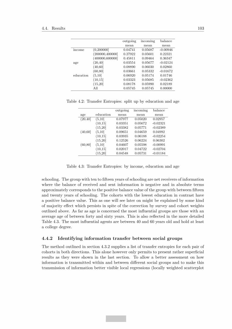
4.4. Results 103
outgoing incoming balancemean mean mean
income (0,200000] 0.04741 0.05687 -0.00946(200000,400000] 0.27922 0.05601 0.22321(400000,600000] 0.45811 0.09464 0.36347
age (20,40] 0.03554 0.05677 -0.02124(40,60] 0.08890 0.06030 0.02860(60,80] 0.03661 0.05332 -0.01672
education (5,10] 0.06920 0.05174 0.01746(10,15] 0.03323 0.05685 -0.02362(15,20] 0.08178 0.05990 0.02189All 0.05745 0.05745 0.00000
Table 4.2: Transfer Entropies: split up by education and age
outgoing incoming balanceage education mean mean mean
(20,40] (5,10] 0.07977 0.05020 0.02957(10,15] 0.03351 0.05672 -0.02321(15,20] 0.03382 0.05771 -0.02389
(40,60] (5,10] 0.09651 0.04659 0.04992(10,15] 0.03935 0.06188 -0.02254(15,20] 0.12526 0.06224 0.06302
(60,80] (5,10] 0.04607 0.05598 -0.00991(10,15] 0.02017 0.04722 -0.02704(15,20] 0.04548 0.05731 -0.01184
Table 4.3: Transfer Entropies: by income, education and age
schooling. The group with ten to fifteen years of schooling are net receivers of informationwhere the balance of received and sent information is negative and in absolute termsapproximately corresponds to the positive balance value of the group with between fifteenand twenty years of schooling. The cohorts with the lowest education in contrast havea positive balance value. This as one will see later on might be explained by some kindof majority effect which persists in spite of the correction by survey and cohort weightsoutlined above. As far as age is concerned the most influential groups are those with anaverage age of between forty and sixty years. This is also reflected in the more detailedTable 4.3. The most influential agents are between 40 and 60 years old and hold at leasta college degree.
4.4.2 Identifying information transfer between social groups
The method outlined in section 4.3.2 supplies a list of transfer entropies for each pair ofcohorts in both directions. This alone however only permits to present rather superficialresults as they were shown in the last section. To allow a better assessment on howinformation is transmitted within and between different social groups and to make thistransmission of information better visible local regressions (locally weighted scatterplot

104 Chapter 4. Expectation Formation and Social Influence
6
8
10
12
14
16
6 8 10 12 14 16
sender education
rece
ive
r e
du
ca
tio
n
0.00
0.05
0.10
0.15
ten.x
Transfer Entropy
Figure 4.1: Information transfer between social groups with different educational back-ground (x-Axis: sender education; y-Axis: receiver education; green: low informationtransfer; red: high information transfer).
smoothing) (Cleveland et al., 1992) are used to fit the estimated transfer entropy valuesto a polynomial surface of degree two determined by sociodemographic characteristics aseducation, income or age. The above described procedure allows to generate continuousheat-maps (also called elevation maps) as in the Figures 4.1, 4.2 and 4.3 which in thiscontext capture the information transmission between social groups of different educa-tional background, different income and different age. The x-axis displays the years ofschooling / income / age of the sending individual (cohort) and the y-axis the educa-tional background / income / age of the receiving individual (cohort). Darker shades ofred represent a higher degree of information transmission from x to y. In regions witha lighter green shade in contrast the information transmission from the x-axis to they-axis is lower. Figure 4.1 suggests that there is a high degree of information transferfrom groups with high education to both groups with lower and higher education. Thismeans that agents with high education are not only net senders of information as wasalready evident by Table 4.2 but are influential beyond their social class. It is howevernoteworthy that this influence is not equal on all social groups. The dark red shades inthe upper right corner suggest some kind of peer effect: Agents with high education pre-dominantly interact with highly educated peers. The degree of information transmissionis accordingly higher within this group.
Figure 4.2 supports the findings of the last section. Social influence here in the

4.4. Results 105
1e+05
2e+05
3e+05
4e+05
1e+05 2e+05 3e+05 4e+05
sender income
rece
ive
r in
co
me
0.2
0.4
0.6
0.8ten.x
Transfer Entropy
Figure 4.2: Information transfer between social groups with different income (x-Axis:sender income; y-Axis: receiver income; green: low information transfer; red: highinformation transfer)
context of expectations with regard to the overall economic development is increasingwith income. Two things are worthwhile to note: First, as far as high income groups areconcerned there also seems to be a peer effect mechanism at work as it is the case foreducation which was discussed above. Second, agents with low income are susceptible toadopt opinions from other social groups. Figure 4.3 finally breaks down the transmissionof information by the age of agents. As was already seen in the last section the mostinfluential agents are between forty and sixty years old. The social influence of thisgroup is not only limited to peers but extends to all age groups. The results presentedabove give a good notion which factors are determining for the degree of social influence.It has to be noted however, that the above used approach is not suited to investigatesub-group effects of variables like education, age or income separately. In reality thereis of course a high coincidence between these characteristics: agents with a higher agetend to have a higher income, agents with higher income tend to have a higher educationetc..
4.4.3 Transfer Entropy and Social Networks
A striking feature of applying information theory to survey data as outlined in sections4.2 and 4.3 is that it not only allows to measure information transmission betweendifferent social groups (some results were presented above) but also to take a closer look

106 Chapter 4. Expectation Formation and Social Influence
30
40
50
60
70
30 40 50 60 70
sender age
rece
ive
r a
ge
0.02
0.04
0.06
0.08
0.10
ten.x
Transfer Entropy
Figure 4.3: Information transfer between social groups with different age (x-Axis: senderage; y-Axis: receiver age; green: low information transfer; red: high information transfer)
at the structure of the underlying network of social influence itself. To do so it is simplyassumed that one cohort x has strong ties to another cohort y if the sum of transferentropies in both directions (Txy + Tyx) surpasses as certain value. In this context wedo so by only looking at highest twenty percent of mutual information flows. Only thenit is assumed that there is a close and stable connection between two agents/cohorts.The result is graphically displayed in Figure 4.4. It is striking that there seems to be ahierarchy between the different vertices (of which each represents a cohort)8: Thus thereare some vertices with a lot of connections while others only have few. Calculating thedegree distribution, this means the cumulative frequencies or probabilities of verticeswith a given degree (number of ties or links) we can investigate the structure of thenetwork. E.g. the P (d) is the fraction of vertices with a degree d. When n is the numberof vertices and P (n) = 1 as well as P (d �= n) = 0 then one speaks of a regular network.In reality networks however rather follow a power-law. This means the probability ofvertices with higher degrees falls exponentially as the number of degrees increases. Inthis case such a network is denoted as a scale-free network: P (d) = cd−γ . Here c > 0 isa scalar and γ is the exponent of the power law (Jackson, 2008, p. 31).
To test if the social network we established by measuring transfer entropies betweeneach pair of cohorts within the Michigan consumer survey also follows a scale free dis-
8Some cohorts dropped out due to the lack of strong connections.

4.4. Results 107
●
●
●
●
●
●
●
●
●
●
●
●
●
●
●
●
●
●
●
●
●
●
●
●
●
●
●
●
●
●
●
●
●
●
●
●
●
●
●
●
●
●
●
●
●
●
●
●
●
●
●
●
●
●
●
●
●
●
●
●
●
●
●
●
Figure 4.4: The network of social influence as estimated by the University of Michiganconsumer Survey
tribution we can simply fit a power-law to the empirical degree distribution.9 Theresult is displayed in Figure 4.5. The estimated value of γ corresponds to 2.3643 . AKolmogorov-Smirnov test with a test statistic of 0.0765 (p-value: 0.9591 ) suggests thatthe hypothesis that the original sample data from the network established by measuringtransfer entropies between pairs of cohorts within the Michigan Consumer Survey couldhave been drawn from the fitted power-law distribution cannot be rejected. It followsthat the estimated network follows a power-law distribution and thus represents a scalefree network. The network inferred by the technique outlined above further exhibits ahigh degree of clustering: The cluster or transitivity coefficient (Wasserman and Faust,1994) is at 0.3426 reflecting a rather high probability that the neighboring vertices of anode are connected as well.
4.4.4 Higher connectivity, more influence
With regard to the results presented in Section 4.4.2 one might ask if the influence ofcertain agents on others is also reflected in their connectivity, namely in the degree ofthe most influential vertices. The transfer entropy alone only measures the informationflow from one agent to another. This means the figures presented until now could havedepended on a few very strong connections. Displaying Figure 4.4 in the form of arcplots
9This was done using the power.law.fit function implemented in the R package “igraph" (Newman,

108 Chapter 4. Expectation Formation and Social Influence
● ● ● ● ● ● ●● ●
● ●●●
●●●●
●●●●●●
●●●●●●
●●●●
●●●●●●●●●●●●●●
●●●●●●●●●●●●●●●●●●●●●●
●●●●●●●●
●●●●●●●●
●●●●●●●●●●●●●●●●●●●●●●
●●●●●●●●●●
●●●●●●●●●●
1 2 5 10 20 50 100
0.0
10.0
50.1
00.5
01.0
05.0
0
Degree
Cum
ula
tive
Fre
quency
Figure 4.5: Cumulative degree distribution with power law fitted (log-scale)
as done in Figure 4.6 has the advantage that one can order the vertices by certaincharacteristics which in turn allows to make assertions about how the characteristicsinfluence the connectivity of the vertices. Figure 4.6 shows that the influence of agentsindeed coincides with very high connectivity: This means the higher the education orthe income of agents the better connected they are. The same is true for higher age.The latter assertion might seem contradictory to the results discussed in section 4.4.2.One has to note however that Figure 4.6 only displays the strongest 20% of connections.Weaker connections were dropped. Therefore not the whole range of age classes (forexample those weaker connected age classes beyond 60 years) are displayed in the plot.
This assessment is further supported when taking a closer look at various central-ity measures for individual vertices. Figure 4.7 displays four centrality measures as afunction of age, education and income:
1. Degree centrality: Degree centrality measures the connectedness of a vertex. In anetwork with n vertices a vertex can have at maximum a degree of n − 1 (i.e. linksto other nodes). The degree centrality measure is then the relation of the degreeof one node i to the number of all other nodes: Ced
i = di(g)/(n − 1). This meansthe higher the centrality of one vertex with respect to its degree is, the closer toone this centrality measure will be.
2. Closeness centrality (Freeman, 1979): This centrality measure is defined as the
2005; Clauset et al., 2009).

4.4. Results 109
● ● ● ● ● ● ● ● ● ● ● ● ● ● ● ● ● ● ● ● ● ● ● ● ● ● ● ● ● ● ● ● ● ● ● ● ● ● ● ● ● ● ● ● ● ● ● ● ● ● ● ● ● ● ● ● ● ● ● ● ● ● ● ●
high education low education● ● ● ● ● ● ● ● ● ● ● ● ● ● ● ● ● ● ● ● ● ● ● ● ● ● ● ● ● ● ● ● ● ● ● ● ● ● ● ● ● ● ● ● ● ● ● ● ● ● ● ● ● ● ● ● ● ● ● ● ● ● ● ●
high income low income
● ● ● ● ● ● ● ● ● ● ● ● ● ● ● ● ● ● ● ● ● ● ● ● ● ● ● ● ● ● ● ● ● ● ● ● ● ● ● ● ● ● ● ● ● ● ● ● ● ● ● ● ● ● ● ● ● ● ● ● ● ● ● ●
higer age lower age
Figure 4.6: The Social Network in the form of ordered arcplots
inverse of the average shortest distance from one vertex to all other vertices. Thusif l(i, j) is the number of links on the shortest path between the vertices i andj, the average distance (number of links) is d(i, j) =
�
i�=j l(i, j)/(n − 1) and thecloseness centrality measure is Cec
i = (n − 1)/�
i�=j l(i, j) =�
i�=j 1/d(i, j).
3. Betweenness centrality (Freeman, 1979): In contrast to the degree and closenesscentrality the betweenness centrality doesn’t measure the centrality of a vertexby the connectedness of a vertex but rather by its role as an intermediator. Thebetweenness centrality of a vertex i is thus the number of shortest paths betweena pair of vertices j and k on which one can find vertex i relative to the number ofall shortest paths between j and k summed over all pairs of vertices. If pjk is thetotal number of paths between two vertices j and k and pjk(i) is the number ofpaths between these two vertices passing through vertex i, betweenness centralityis defined as: Ceb
i =�
i�=j �=k pjk(i)/pjk.
4. Eigenvector centrality (Bonacich, 1987): This measure considers not only the con-

110 Chapter 4. Expectation Formation and Social Influence
nectedness of a vertex but also the connectedness of its neighbors. The centralitytherefore not only depends on the links a vertex has but also on how central itsneighbors are within the network. If A is the adjacency matrix of the networkN where its elements ai,j ∈ {0, 1} indicate the presence of a link (0 no link; 1link) between two vertices i and j, and M(i) is the set of neighbors of vertex i,the eigenvector centrality of a vertex is the sum of the centralities of its neighborsmultiplied by a constant 1
λ: Ce
i = 1λ
�
j∈M(i) Cej = 1
λ
�
i∈N ai,jCej . Rearranged in
matrix form one gets the eigenvector equation Ax = λx which is eponymous forthis centrality measure.
The different centrality measures formally outlined above capture different notions ofcentrality. Degree centrality is the simplest concept, reflecting the number of links of anode or vertex. In a directed network, this means if the assumption is made that theedges between vertices are directed, one can further differentiate between the out- orin-degree, i.e. the number of links departing from or arriving at a node. In the contextof this study only the overall degree, thus the sum of in- and out-degrees of a node isconsidered. As outlined above closeness centrality corresponds to the sum of all shortestpaths from a specific node to all other nodes. This sum is the lower the more central anode is. Closeness centrality is considered a measure which reflects the importance ofan agent spreading information or in other contexts, a disease. Betweenness centralityin contrast measures the importance of a node as an intermediator. It thus measureshow many times a node appears on the shortest paths between all other nodes and towhat extent a specific node is in control of the communication between other nodes.Eigenvector centrality corresponds to the eigenvalues of nodes in the adjacency matrix.It thus reflects the centrality of a node in relation to the centrality of other nodes towhich it is linked. The score of a specific node is the higher, the higher the score ofconnected nodes is. The Eigenvector centrality thus represents a reciprocal measure ofconnectedness. (Tanaka et al., 2013; Borgatti, 2005).
The curves in Figure 4.7 were generated by calculating the various centrality mea-sures discussed above for each vertex and interpolating these values with respect to age,education and income using local regressions (Cleveland et al., 1992). The results sup-port the conclusion from above: As far as age is concerned the centrality of an agentwithin a network of social influence around the age of fifty. The centrality of an agentalso increases with income and is the highest at a yearly income of around USD 30,000.The interpretation is however not that conclusive when looking at the graphs displayingthe centrality measures as a function of schooling years. Similar to Figure 4.1 the socialinfluence and therefore the centralities of vertices reach their climax between fourteenand sixteen years of education. The centrality measures are however nearly as high forgroups with lower education, a phenomenon potentially explicable by a majority effectwhich appears despite of correcting for survey and cohort weights.

4.4. Results 111
30 40 50 60 70
30
60
de
gre
e
30 40 50 60 70
03
0
be
twe
en
ess
30 40 50 60 70
0.4
0.6
eig
enve
cto
r
30 40 50 60 70
0.0
09
0
age
clo
se
ne
ss
6 8 10 12 14 16
20
60
6 8 10 12 14 16
03
06
0
6 8 10 12 14 16
0.2
0.6
6 8 10 12 14 16
0.0
08
0.0
12
years of schooling
0e+00 2e+05 4e+05
40
12
0
0e+00 2e+05 4e+05
01
00
0e+00 2e+05 4e+05
0.4
0.8
0 200000 400000
0.0
10
0.0
18
yearly income in USD
Figure 4.7: Degree, betweenness, eigenvector, closeness centrality as a function of age,education and yearly income in USD

112 Chapter 4. Expectation Formation and Social Influence
4.4.5 Information transfer over time
Figure 4.8 displays the measured transfer entropies with respect to education, age and in-come as a function of time. In contrast to before here the width of the time bin k (outlinedin section 4.2) which used to be one month for the results presented above is now variedbetween one and twelve months. This means while we before only paid attention to thecontributions in terms of predictability from yt to xt+1 that is H(xt+1|xt)−H(xt+1|xt, yt)we now instead extend the signal length and look at H(xt+1|xk
t ) − H(xt+1|xkt , yk
t ) wherexk
t = xt, . . . , xt−k+1, ykt = yt, . . . , yt−k+1 and k ∈ 1, . . . , 12.
Extending the signal length into the past shows that the information transfer onaverage sharply increases until k = 3 and slowly decreases for higher bin widths. Asalready seen in Figures 4.1 to 4.3 influence increases with education as well as income.As far as age is concerned one observes a clear peak at age groups between forty and sixtyyears. The decline of the transfer entropies when extending the signal length beyondk = 3 is approximately equivalent over all groups.
education
time
TI
age
time
TI
income
time
TI
Figure 4.8: Information Transfer under consideration of different time lags

4.5. Conclusion 113
4.5 Conclusion
This paper presents a way to apply information theory namely the concept of transfer en-tropy by Schreiber (2000) to consumer surveys. Using self-organizing Kohonen maps therepeated cross-section structure of the University of Michigan consumer survey data setwas transformed into a pseudo-panel with 64 cells. Subsequently the information theo-retic measure of transfer entropy was used to measure the mutual (i.e. in both directions)information flow between all pairs of cohorts in the context of business expectations. Itwas shown that social influence is strongly determined by the sociodemographic situa-tion of an agent: Social influence on other agents increases with education and income.As far as age is concerned agents between forty and sixty years are the opinion leadersexerting influence on other groups.
Looking only at the strongest ties in terms of mutual information transfer between thedifferent cohorts within the University of Michigan survey data set allows to assess theunderlying network structure. It turns out that the inferred network of social influenceis scale-free and follows a power-law with an exponent γ of 2.3643. This means thenumber of agents falls exponentially with the number of their degrees. Such a networkstructure is realistic and often observed in other contexts. We further saw that highinfluence coincides with high connectivity. This means that highly influential agentsexert their influence not only on a few other cohorts but play a central role within thenetwork structure. This conclusion can also be drawn when plotting measures as degree,betweenness, closeness and eigenvector centralities against variables as age, educationor income: The high degree of social influence by certain groups strongly relies on theircentral positions within the network of social influence. These respective groups are notonly generally well connected but also play important roles as intermediators and areparts of influential cliques. It is further shown that social influence reaches its peak ata bin width of three months of past data but diminishes beyond this point.

114 Chapter 4. Expectation Formation and Social Influence

Chapter 5
A Concept for Constructing anEconomic Sentiment Indicator viaWeb Mining
5.1 Objective
Economic Sentiment Indicators have developed into helpful supplementary tools tosurveil, analyze and forecast aggregate economic fluctuations in the short run. Tra-ditionally they base on surveys evaluating opinions and expectations of economic agentsregarding economic prospects or perceptions of past economic evolutions on a regularbasis. Under the assumption that the internet nowadays serves as a large reservoir forthe expression of opinions and expectations, this research project aims to construct aneconomic sentiment indicator analyzing unstructured textual data which is freely avail-able on the internet making use of modern text and sentiment mining technologies incombination with traditional econometric analysis. The proposed web-based sentimentindicator will be able to deliver more up-to-date sentiment information than the tradi-tional monthly survey based sentiment indicators, which allows to track economic trendsas they are emerging.
5.2 Background and Context
Beginning with the seminal works of Knight (1921) and Keynes (1936) decision makingof economic agents is considered to be shaped by expectations and the assessment of riskreflecting among other things psychological aspects (Carnazza and Parigi, 2002). Basingon these theoretical foundations precursors of modern day Behavioral Economics likeGeorge Katona committed themselves to construct and develop instruments measuringattitudes and expectations of economic agents towards the economy. The results of thiswork emerged in the creation of typically survey based indicators in the early post warperiod, which focused on consumer and business confidence and established themselves
115

116Chapter 5. A Concept for Constructing an Economic Sentiment Indicator via Web
Mining
as important supplements to macroeconomic data in forecasting and evaluating trendsin the evolution of the economy (Katona, 1974). Early and well known proponents ofindicators directed at households are e.g. the University of Michigan Consumer Sen-timent Index (MCSI)1, conceptualized by George Katona and regularly updated since1955, or the Consumer Confidence Index (CCI), which started in 1967 and is since thenupdated and maintained by the U.S. Conference Board. Later on the concept of surveybased assessment of economic sentiment was extended to businesses as in the form of thePhiladelphia Fed Index, which is conducted since 1968, or the German IFO Business Cli-mate index, which has its roots in the late 1940s and is regularly measured and publishedsince 1972. Similar approaches to assess economic sentiment are nowadays applied in allmajor economies. Partly sentiment indicators are bundled or enriched with macro-datato allow for a better evaluation of future economic prospects. An example for such acomposite index, which combines the survey results from different industries and coun-tries, is the European Economic Sentiment Indicator (ESI) directed by the EuropeanCommission. A special form of sentiment indices represent the surveys of professionalforecasters, as e.g. the Philadelphia Fed’s Survey of Professional Forecasters, concerningthe evolution of macroeconomic variables.
All aforementioned indices have in common that they use a survey design to evaluatethe assessment of economic prospects with respect to the current economic situation.Households e.g. might be asked how they expect their income to change within a certainperiod in comparison to the moment of the survey. Businesses might be surveyed howthey judge their inventory holdings or how they expect their order books to evolve.The respondent is however not asked to give precise quantitative answers but ratherto choose one out of different qualitative and ordered answering options, e.g. did theorder situation improve, stay the same, did it get worse. In the simplest case the sogained qualitative results are converted into quantitative, aggregate sentiment data bysetting the proportions of optimistic and pessimistic answers into relation. Fluctuationsaround the scaled long term average can then be used to make assertions over theconfidence of households or businesses (Carlson and Parkin, 1975; Pesaran, 1984)2. Thequalitative, expectation and opinion focused design of the above mentioned indices standsin contrast to a second category of indices which asks for factual information ratherthan expectations or opinions. As an example for this group the numerous PurchasingManager Indices can be mentioned (Pesaran and Weale, 2006b).
Consumer sentiment and business sentiment indicators enjoy, due to their good pre-dictive properties and their function as leading indicators for macro-data, which can onlybe measured in bigger time intervals, great popularity among business cycle researchersand professionals in the financial industry. Various empirical studies prove this features,e.g.: Mourougane and Roma (2003) study the predictive power of the ESI for the shortterm real GDP growth in different European economies. Ludvigson (2004) shows thatconsumer sentiment is a good predictor for consumer spending. Howrey (2001) demon-strates that consumer sentiment captured by the MCSI can serve as a good predictor
1Data from the MCSI was used in Chapters 3 and 4)2More sophisticated quantification results were discussed and applied in Chapters 2 and 3.

5.3. Significance of the Study 117
for real GDP growth. Vuchelen (2004) follows a similar approach and comes to ana-log results in the Belgium context. Grisse (2009) studies the feedback effect which caneventually arise by publishing business confidence indices, rendering the so measuredexpectations to be self-fulfilling prophecies of economic prospects.
5.3 Significance of the Study
The spread and development of internet technologies as well as the increased user-friendliness of web applications in the recent years has transformed the web from atool which initially served mainly the passive consumption of information into a vehicleto share opinions with others and to participate in the discourse about every thinkableissue. The web 2.0, as it is referred to occasionally in media, allows users without furthertechnological knowledge to interactively exchange information and in this sense also toutter mood and sentiment, be it in blogs, reviews or newsgroup messages. It seemstherefore reasonable to fathom the potential of sentiment information stored in unstruc-tured textual information on the web to study expectation formation in the context ofbusiness cycle research and to forecast economic trends.
The above described evolution of web technologies and the change of their employ-ment lead computer scientists, mainly motivated by the economic interest of businesses,to develop technologies to systematically analyze, classify and quantify the vast, everincreasing amount of mainly textual and therefore unstructured information. The com-bination of traditional linguistic methods of text analysis with improving capacitiesregarding software, processing power, the further development of machine learning al-gorithms as well as the availability of training corpora3 contributed crucially to theenormous progress in this respect and culminated into the very active research field ofsentiment or opinion mining respectively. The employment of these techniques allowsbusinesses to semi-automatically evaluate costumer reviews, feedback and opinions inorder to more efficiently account for their preferences in the context of reputation man-agement or to compile forecasts concerning trends in order to enhance their chancesin the market (Mishne and Glance, 2006; Lee, 2004). Policymakers take advantages ofopinion mining technologies to evaluate public opinion considering pending law or regu-lation proposals. This subfield is denoted as “eRulemaking” (Cardie et al., 2006; Kwonet al., 2006).
The applications of these techniques in an economic context are yet relatively rarethough quite promising. The only works to which in the broader sense a principlesimilarity can be attributed to the approach envisaged for this project, are those byTims et al. (1989), Blood and Phillips (1995), Fan and Cook (2003) as well as Domsand Morin (2004). Above mentioned articles find that economic news coverage has
3A Corpus denotes a structured set of texts which e.g. can be used to experiment with machinelearning algorithms to automatically classify texts by topic or polarity (sentiment). A well knowntraining corpus is the Reuters RCV1 corpus distributed by the National Institute of Standards andTechnology which contains several hundred thousands newswire articles published by the news agencyReuters to which meta informations as e.g. place and subjects were attributed by hand.

118Chapter 5. A Concept for Constructing an Economic Sentiment Indicator via Web
Mining
significant influence on consumer sentiment. Doms and Morin (2004) for example showthat the appearance of negatively connotated expressions like recession and slowdownin news coverage about economic topics has significant explanatory power for decreasesin consumer confidence. Starr (2012) confirms the coherence of consumer sentimentand news coverage using surveys in the context of the data collection for the MichiganSurvey of Consumer Attitudes. This empirical literature indirectly references the idea ofthe theoretical literature on Pigou-Cycles which explains the cyclical movement of theeconomy by positive news shocks, leading to economic boom phases which result into abust when it turns out that expectations where too optimistic. These ideas, originallydeveloped by Arthur Pigou (1929) in the 1920s, recently experienced a renaissance inliterature as there is evidence to suggest that similar mechanisms played a role in theemergence and bust of the dot-com bubble in the 1990s where markets overestimatedthe potential of new internet technologies (Beaudry and Portier, 2004; Collard, 1983;Beaudry and Portier, 2006; Jaimovich and Rebelo, 2009). The high degree of optimismin this time is also reflected in the consumer sentiment and business confidence data ofthis period (Mehkari, 2010). The above cited works however don’t take advantage ofthe computerized sentiment mining techniques which are envisaged for this project, butrather come to their results through manual data collection and traditional quantitativemethods. They nevertheless indicate the following points, which are central assumptionsfor the here presented research project: First, textual information can be a carrier foreconomic sentiment. Second, a less trivial conclusion, the impact of this sentiment canbe measured.
That news and written communication in general have an impact on market expec-tations can also be shown from another direction, which suggests that computerizedtext mining could be an appropriate tool for the detection of economic sentiment butalso illustrates a potential strategy for the project to construct an Economic SentimentIndicator by analyzing unstructured textual data published on the web. Koppel andShtrimberg (2006) e.g. suggest a method to automatically categorize news stories intonegative or positive polarity by the impact they have on stock market movements. Intheir article the authors examine a corpus of 12,000 news articles between the years2000 and 2002 concerning items within the Standard & Poor 500 (S&P500) stock mar-ket index which corresponds to around 24 news stories on each asset. By looking atthe stock movements within a certain time frame after publication, the news articleswere categorized into groups with negative and positive impact respectively. For the up-ward (positive) and downward (negative) movements respectively threshold values werechosen to assure that the changes don’t simply reflect random fluctuations or normalmarket movements. Further it was defined that the respective items have to have a min-imum value and that the percentage alteration of the prices in question has to exceedthe percentage change of the S&P500 index within the same time period. Then binaryword frequency vectors were compiled in which irrelevant function words were pruned.Consequentially learning algorithms like Support Vector Machine (SVM), Naïve Bayesand Decision Trees were used to learn the text and word patterns connected with thepolarity respectively. A tenfold cross-validation experiment, in which it was tested to
5.3. Significance of the Study 119
what extent the learned text pattern were applicable to categorize articles, yielded aclassification accuracy of around 70% (Koppel and Shtrimberg, 2006). This supportson the one hand the results of the other literature cited above, namely that there is arelevant and significant connection between news and expectations which influence mar-kets, on the other hand the experiment by Koppel and Shtrimberg shows that learningalgorithms can be used to recognize sentiment patterns in text which can influence thebehavior of economic agents.
Another interesting approach to use text and sentiment mining techniques in contextof economic problems comes from Ghose et al. (2007). Ghose et al. (2007) investigateby the application of text mining in combination with econometric methods, if the pos-itive/negative sentiments uttered in costumer reviews on the online market platformwww.amazon.com have an effect on the price premium sellers could take, respectively ifone could infer a positive/negative polarity of expressed opinion by the pricing power ofa seller. Therefore the authors identify dimensions of reputation which are importantfor the evaluation of the services a seller offers. Such dimensions could be e.g. delivery,packaging, costumer support etc. By the use of a natural language processing algorithm(NLP) parser (this parser is an algorithm to identify parts of speech (POS) as nouns,verbs, adjectives and adverbs and sets them into relation to each other) the authors findmodifiers of these dimension. If one for example considers the dimension “delivery”,which is the noun along the POS scheme, the adjective “speedy” would be a modifier.Parsing out the modifiers for every dimension from the customer reviews regarding aseller yields a dimension/modifier matrix for each merchant. By weighting with respectto dimension and time of the reviews, newer reviews are weighted higher than olderreviews, a virtual reputation score for each merchant is calculated. Then after panelOLS-regressions with fixed effects were run where the impact of the independent vari-able, the reputation scores of two competitors within one market (additionally to thatthe www.amazon.com star rating system, the number of past transaction and the numberof sellers in the market were used as control variables), for the dependent variable, thecharged price premium, was estimated. The resulting significant coefficients for severalmodifier-dimension pairs can then be calculated, with the weightings, and interpreted inmonetary terms. The study of Ghose et al. (2007) yields two important results: First,it demonstrates that sentiment and opinion have a measurable condensation in unstruc-tured textual data, second and more importantly, economic agents absorb subjectiveexperiences of others and consider it in their decision making as reflected by the effectof enhanced pricing power for merchants with good reputation.
A commanding impression which potential user generated data on the internet hasfor economic forecasting, even if to lesser extent connected with the field of sentimentmining, delivers the paper by Schmidt and Vosen (2009). Under the assumption thatmore and more customers use the internet as a research instrument in preparation ofacquisitions, the authors use data provided by the search engine Google in the context ofthe Insights for Search application about search terms entered by users to forecast privateconsumption. It is shown that both with and without combination of other macro-datathe Google-Trends data exhibits a higher predictive power for private consumption than

120Chapter 5. A Concept for Constructing an Economic Sentiment Indicator via Web
Mining
traditional, survey based consumer sentiment indicators as the MCSI and the ConferenceBoard Consumer Confidence Index.
Last but not least the work by Hal Varian has to be mentioned in this context. Hewas one of the first in the Economic profession to realize which impact web technologieswould have for the business life and the field of Economics. Noteworthy in this regard ishis famous book “Information rules: a strategic guide to the network economy”(Varianand Shapiro, 1999) coauthored with Carl Shapiro. Currently holding the position ofGoogles chief economist he is one of the most visible proponents of combining webtechnologies and data mining with traditional econometric methods. Especially his worktogether with Choi received significant attention, in which the authors demonstrate,similar to the above cited article by Schmidt and Vosen (2009), the impressive propertiesof Google Trend data to forecast inter alia automobile sales, unemployment claims andconsumer confidence (Choi and Varian, 2012). In his article “Big data: New tricks foreconometrics” Varian gives an overview of applications of machine learning to big datain an economic context (Varian, 2014). Of special interest for econometricians is therebyhis discussion of Bayesian Structural Time Series analysis with feature selection, whichis used to choose the best predictors for home sales figures from a wide variety of Googlequery time series data. The initial set of predictors was hereby chosen using the GoogleCorrelate tool, which allows to submit a time series and returns hundred queries which,in terms of search frequencies, have the highest correlation with the originally uploadedtime series. Likewise appealing is his outline of model averaging, a method widelyused in machine learning but relatively new to Econometrics, to enhance predictionquality. Varian however also points out a weakness of machine learning techniques forthe application in Economics: Algorithms like random forests can be extremely complexand thus very difficult to interpret (Varian, 2014, p. 15). A good overview of recentapplications of machine learning techniques in Economics is given by Einav and Levin(2013).
This section sketched the potential of using computerized sentiment mining for eco-nomic sentiment analysis: With reference to examples from literature it was shown thattext mining technologies applied on unstructured textual data have the ability to parseout sentiments which can be set into an economic context, meaning that the impact oneconomic behavior of analyzed sentiment can be measured and is significant. The usein economic problem fields, especially on an aggregate level, is however rare or inexis-tent respectively. The next section is dedicated to outline a strategy how an economicsentiment indicator measuring consumer and business confidence following the exam-ple of survey based indicators can be constructed using computerized sentiment miningtechniques on unstructured textual data published on the internet.
5.4 Methodology
The principle procedure to construct a web based economic sentiment indicator is asfollows: Given a sufficiently large training corpus with documents which are annotatedwith regard to topics and sentiment, text mining techniques can be used to make these

5.4. Methodology 121
Figure 5.1: Flowchart of the Procedure
documents machine readable. With the annotated training corpus and the use of ma-chine learning algorithms the computer can be taught to recognize the specific patternscharacterizing for textual documents and to automatically categorize new texts, whichwere parsed out from the web, along the predefined annotation schemes e.g. topics andsentiment. This results into time- and topic-referenced sentiment information, similar tothe sentiment information extracted by surveys, which can be used to construct a sen-timent indicator reflecting economic confidence and trends. In the following the stepsand elements necessary to construct a web-based economic sentiment indicator based onanalyzing textual information on the internet via text mining will be described in moredetail. The procedure is schematically displayed with a flowchart in Figure 5.1.
5.4.1 Data Sources and Collection
The sources which can be potentially used for the construction of a web based EconomicSentiment Indicator as envisaged here are manifold as there is a huge, ever increasingamount of textual data available on the internet. Two points are however crucial: First,the examined articles have to have a time stamp. This means the date and time whenthe article was published must be known and parsable. Second, the originality of thearticle must be assured. This means it would for example make no sense to read out newsinformation of several english speaking online newspapers about a certain topic knowingthat they are most probably just copied versions of articles bought from press agenciesas e.g. Reuters. Considerable information sources would therefore be newswire articlesfrom press agencies directly, blogs, news group articles or even short message services.It might also be interesting to take a look at so called news crawlers or news feeds as

122Chapter 5. A Concept for Constructing an Economic Sentiment Indicator via Web
Mining
sources. These are websites and applications respectively which parse out articles fromdifferent websites about certain topics. The probably most comprehensive newsfeedis the news feed provided by google.com. The advantage of news feeds is that theydeliver textual content already in categorized form. Important to mention is howeverthat the project foremost concentrates on resources from the English speaking world:First, because there is a by far greater variety of text mining algorithms for the Englishlanguage than for any other language, second but not least, because the publicationwill be in English. The same methods though can of course be broadened to any otherlanguage.
For the purpose of experimentation and training of the envisaged model there areseveral training corpora available. This facilitates the project insofar as for the calibra-tion and testing of the model no data has to be retrieved from the internet which can betime and resource consuming. The most appropriated corpora for the here envisionedpurpose seem to be the Reuters RCV1, this corpus contains 810,000 newswire articlesfrom Reuters between 1996 and 1997 and is distributed by the National Institute ofStandards and Technology (Lewis et al., 2004), and the TREC BLOG06 test collection,which is a corpus of several million blog documents and news feeds from 2005 to 2006collected and distributed by the University of Glasgow (Ounis et al., 2008). Advanta-geous features of the RCV1 corpus are e.g. that it is freely available and that documentsare in the hierarchic XML language which makes it easy to parse out necessary anduseful information as publication time, places and topics. These are the reasons why theRCV1 corpus was used in the experimental crowd sourcing platform which was set upto create an annotated training corpus and will be presented later on.
There are however many other suitable corpora. Noteworthy are for example theNew York Times Annotated Corpus, which contains 1.8 million New York Times articlespublished between 1987 and 2007 (Sandhaus, 2008). A huge advantage of this collection(like with the RCV1 corpus) is, as will be clearer later on, that the articles were annotatedby humans. This means every article contains labels and tags regarding topics and places,etc., which were systematically attributed by the NYT staff.
5.4.2 Text mining
Text mining in its basic sense is an umbrella term for computer linguistic methods tosystematically organize weakly structured textual information in a way that it is opento numerical statistical analysis and readable for machines. All further on describedtasks are standard applications in available text mining software packages. Taken thata collection of documents, a corpus, should be analyzed, a text mining project normallybegins with splitting up the individual texts into words denominated as tokens. Thisprocess is named tokenization and ultimately pursues the objective to compile a termfrequency matrix which makes the corpus readable for machines and allows the autom-atized comparison and analysis of different documents in the corpus. A term frequencymatrix indicates if or how often a certain parsed out term, a token, occurs in a certaindocument within a corpus. A corpus containing n documents and overall m tokens wouldtherefore result in a n×m term frequency matrix (see for example Table 5.1). The above

5.4. Methodology 123
word 1 word 2 word 3 ... word m labeldocument 1 0 1 1 ... 1 .document 2 1 0 0 ... 0 .document 3 0 0 1 ... 0 .
......
......
......
...document n 1 0 1 ... 1 .
Table 5.1: Example of a binary term matrix
described procedure alone would however result into a huge data set, which not least dueto redundancies yields just marginal gains of information.: If for example a corpus ofEnglish documents is big enough, it is reasonable to assume that a term frequency ma-trix would have to capture a sizable fraction of the vocabulary of the English language.Due to inflections, declension and conjugations, it would additionally contain severalforms of the same word. Because of all this, tokenization is usually followed by a row ofother procedures to reduce data amount drastically. These procedures involve filtering,pruning and stemming algorithms. One might for example want to filter out stop-wordsas “the”, “this” or “an” which are regarded to have no informational content. Addition-ally tokens are also filtered or pruned by their frequency, be it in absolute or fractionalterms, since this could bias the results gained by the application of machine learningprocedures (to be discussed later on): One could for example easily come to the conclu-sion that the appearance of the very frequent token “be” is not a very distinctive featurefor an English text document. Tokens which appear on the other hand very seldom,like names, might also yield no informational gain. Another filtering method is e.g. thelexical substitution of synonyms to avoid redundancies. The most complex procedure ofdata reduction is however stemming. Stemming intends to reduce the parsed out tokensto their morphological roots. Instead of capturing for example both words “fisher” and“fishing” in a term frequency matrix, one would prefer to measure only the occurrenceof there common root “fish”. There are two main types of stemming algorithms: Bruteforce or lexical algorithms on the one hand use lookup tables to substitute tokens bytheir respective morphological roots. Suffix-stripping algorithms on the other hand useinflection rules to cut suffixes from words, e.g. the word “gone” would appear by it’s root“go” in the term frequency table. Brute force algorithm are regarded as more preciseespecially as they have hardly problems with irregular inflections. They are howeververy complex to maintain and resource consuming in their application. In contrast tothat, suffix-strippers are quite efficient with the downside that they have problems withirregularities. For most of the tasks in the context of machine learning and text similari-ties as relevant for the here envisaged project their capacities are however sufficient. Onewell known and widely applied algorithm of this type is the Snowball-Stemmer (Porter,2001; Weiss et al., 2005).
Having conducted the above described preparatory procedures (which proceduresare applied to which extent of course depends on the research interest) a term frequencymatrix can be compiled. This renders the unstructured textual information readable for

124Chapter 5. A Concept for Constructing an Economic Sentiment Indicator via Web
Mining
machines. Machine learning algorithms, these algorithms will be discussed in the nextsection, can then be applied in order to detect patterns and conduct automatized cate-gorization. Table 5.1 displays an exemplary term-frequency matrix with binary values.Other forms of term-frequency matrices display the absolute numerical occurrence of aterm. In a third variant the term frequency - inverse document frequency, the so-calledTF-IDF score, is calculated. This means that terms are counted but down-weightedif they appear in many documents and up-weighted if they appear relatively seldom.4
Other concepts of term frequency tables count n-grams, which are sequences of n tokens,instead of terms, which are considered to be uni-grams along this approach. For morespecified categorization purposes part of speech tagging in combination with simple to-kenization can be considered. Most of the major text mining software applications areable to recognize the role of a word within a sentence. This means they can distinguishif parsed out tokens are e.g. nouns, verbs, adjectives, etc.. If one wants e.g. to categorizedocuments with regard to the topics they are covering, one might find it more appropriateto apply machine learning algorithms on nouns only since the occurrence of verbs is lesscontext dependent. Allowing for all parts of speech in a text categorization procedurecan lead to a lower accuracy. This phenomenon is denoted as “over-fitting”.(Masuyamaand Nakagawa, 2004; Weiss et al., 2005)
5.4.3 Machine Learning Algorithms
Machine Learning algorithms are the core of every sentiment mining project. They havethe ability to recognize patterns and categorize documents into preset categories, beit topics, places or polarities (sentiments). The issue of machine learning algorithmswas already briefly touched in the sections above where the potential of text miningfor economic sentiment analysis was discussed. The principle of the four most popularmachine learning approaches, support vector machines (SVM), Naïve Bayes, decisiontree classifiers and Artificial Neural Networks shall be shortly addressed in the sectionthat follows.
Support Vector Machine The most widely applied machine learning algorithm isthe support vector machine (SVM) approach. Its concept is depicted in Figure 5.2. Thegoal of the SVM in the linear case is to find a hyperplane, which efficiently separatesthe positive sample from the negative sample, depicted by the black and white dotsrespectively. Such a separation rule can then be used to categorize yet unlabeled samples.Given a set of training data D = {(xi, yi)|xi ∈ R
d, yi ∈ {−1, 1}}ni=1 with i = 1, ..., n,
where the label yi ∈ {−1, 1} describes to which category the d-dimensional vector xi
belongs, the SVM calculates the optimal hyperplane w · x − b = 0 which delivers themaximum margin to the positive and negative sample respectively. The margins aredefined to be the distances d+ (d−) from the optimal hyperplane to the closest pointof the positive (negative) sample. w is normal to the hyperplane, and b/�w� with �w�,
4If tf(j) is the overall frequency of term j in N documents, and df(j) gives the number of documentsin which the term j appears, then tf-idf(j) = tf(j) log( N
df(j)).

5.4. Methodology 125
Figure 5.2: Principle of SVM
the Euclidean norm of w, describes the perpendicular distance from the hyperplane tothe origin. The SVM now sets w and b in order to maximize the overall margin d+ +d−. Differently put, the SVM maximizes the distance between the parallel hyperplanesw · xi − b = 1 and w · xi − b = −1, denoted as the “support vectors”, which are stillbarely separating the two samples. The distance between these two “support vectors” is
2�w� . The task is therefore to minimize �w�. Since it is clearly not desirable that pointsare falling into the margin one can redefine the “support vectors” to w · xi − b � 1 andw · xi − b � −1 respectively, which in combination can be rewritten to the constraintyi(w · xi − b) � 1. The problem can then be written down as a quadratic programmingproblem minw,b �w� s.t. yi(w ·xi −b) � 1 ∀i = 1, ..., n or, for the sake of conveniencebut without altering the result, as minw,b
12�w�2 s.t. yi(w · xi − b) � 1 ∀i = 1, ..., n
(�w� is the norm of w and thus contains a square root, which is hard to minimize). Byintroducing a positive Lagrange multiplier αi for i = 1, ..., n, the problem can be denotedin an easier to handle Lagrangian formulation:
L = minw,b
maxa
{12
�w�2 −n�
i=1
αi[yi(w · xi − b) − 1]}
Since the sub condition is set to equality, it is thus required that, subject to the constraintαi � 0, L is minimized with respect to w and b while the derivatives of L with respectto αi have to disappear. It can be shown that the solution w can be expressed as alinear combination of the training vectors xi, w =
�ni=1 αiyixi. From this and the sub
condition of the minimization problem set to equality, yi(w ·xi −b) = 1, b can be derived

126Chapter 5. A Concept for Constructing an Economic Sentiment Indicator via Web
Mining
as b = w ·xi −yi. Equivalently one can write the optimization problem, using the resultsfrom before and the fact that �w� = w · w, as
maxαi
L =n�
i=1
αi −12
�
i,j
αiαjyiyjxTi xj =
n�
i=1
αi −12
�
i,j
αiαjyiyjk(xixj)
s.t.
αi � 0n�
i=1
αiyi = 0 (the constraint minimizing w.r.t. b ∀i = 1, ..., n)
The function k(·) is the kernel defined as k(xi, xj) = xi · xj . If no hyperplane can befound to separate the samples, a soft margin can be implemented by introducing a slackvariable ξi into the classification constraint to allow a certain degree of misclassification:yi(w ·xi −b) � 1−ξi ∀ i = 1, ..., 0. The general procedure stays the same with a slackvariable. The slack variable ξi is just an additional variable with respect to which one hasto minimize. Non-linear classification problems can be solved by mapping the separationproblem into a higher dimensional Euclidean space using alternative kernel functionsk(·). For multiple classification classes, more than two, one could choose a stepwiseprocedure by breaking down the problem into several dual classification problems andclassifying each class in comparison with all others classes, or by pairwise coupling,namely by classifying each class with respect to each other class. Other approaches,like the Decision Directed Acyclic Graph (DDAG) or the Directed Acyclic Graph SVM(DAGSVM) algorithms, try to combine many standard SVM dual-class classifiers intoone algorithm.(Burges, 1998; Taira, 2002; Duan and Keerthi, 2005; Piatt et al., 2000)
Naïve Bayes A second type of classifiers is the Naïve Bayes classifiers. Naïve Bayesalgorithms are simple, resource saving and though very efficient. They are for examplewidely used for filtering out spam E-Mails. A Bayes Classifier along Bayes’ Theoremis in its purest form a function f which maps a vector X of a n-dimensional feature-space into a set of classes Y : f : X ∈ R
n → Y . It is assumed that Y is a boolean-valued random variable and that X is a vector comprising n boolean features, thusX = {X1, ..., Xi, ..., XN }. With respect to the here considered text classification onecould assume that a document, which is characterized by the possible occurrence of ndifferent words X, should be classified into different classes e.g. Y ∈ {spam, no−spam}.Bayes’ Theorem states that
P (X, Y ) = P (X|Y )P (Y ) = P (Y |X)P (X)
Where P (X) is the evidence (distribution of features in the n-dimensional feature space),P (Y ) the prior probability for class Y , P (Y |X) the posterior probability for Y with re-spect to X and P (X|Y ) the class conditional likelihood. Therefore the posterior proba-bility can be expressed by,
P (Y |X) =P (X|Y )P (Y )
P (X)=
P (X|Y )P (Y )�
Y � P (X|Y �)P (Y �)

5.4. Methodology 127
Since P (X) =�
Y � P (X|Y �)P (Y �) as P (X) can be regarded as the marginal value ofP (X|Y ) with respect to Y . Thus actually only the numerator of the posterior probabilityformula is of interest. The Bayes classification problem therefore can be denoted as
Y ∗ = arg maxY
P (Y |X) = arg maxY
P (X|Y )P (Y )P (X)
= arg maxY
P (X|Y )P (Y )
To ensure the pure Bayes Classifier works efficiently, it has to be trained with a suffi-ciently big training sample. To stick to the spam-filter example, this means that theuser has to tag a sufficiently high number of E-Mails as “spam” or “not spam”. In thecase of the spam-filter one can assume that Y is a boolean variable and X exhibits nboolean attributes (words). This implies that X can take on 2n and Y can take on 2values. One has to note that by probabilistic rules it has to hold that
�nXi
P (Xi|Y ) = 1.This implies for every value Y can take, one has to estimate 2n − 1 parameters. If Y isboolean, as in the spam-filter example, one has to therefore estimate 2(2n − 1) parame-ters. To get reliable estimates (frequencies) one has to conduct the estimation procedureseveral times. Thus under the assumption of n = 50, rather unrealistic with regard tospam-filters, one would have to tag several billion E-Mails in order to get a reasonablyreliable spam-filter. This is were the idea of Naïve Bayes classifiers sets in. The NaïveBayes classifier, in contrast to the pure Bayes classifier sketched above, makes the naiveassumption that features Xi and Xj for all i �= j are conditionally independent. Thisimplies that P (Xi|Y, Xj) = P (Xi|Y ) ∀i �= j. Along this assumption the formula forthe posterior probability can be rewritten: The numerator P (X1, ..., Xn|Y )P (Y ) can besimply denoted as the joint probability P (Y, X1, ..., Xn). Applying the chain rule, thejoint probability P (Y, X1, ..., Xn) can be rewritten in the following way:
P (Y, X1, ..., Xn)
= P (Y ) · P (X1, ..., Xn|Y )
= P (Y ) · P (X1|Y ) · P (X2, ..., Xn|Y, X1)
= P (Y ) · P (X1|Y ) · P (X2|Y, X1) · P (X3, ..., Xn|Y, X1, X2)
= P (Y ) · P (X1|Y ) · P (X2|Y, X1) · P (X3|Y, X1, X2) · P (X4, ..., Xn|Y, X1, X2, X3)
. . .
= P (Y ) · P (X1|Y ) · P (X2|Y, X1) · . . . · P (Xn|Y, X1, . . . , Xn−1)
Taken the assumption of conditional independence from before the joint probabilityP (Y, X1, ..., Xn) can be rewritten to the form P (Y, X1, ..., Xn) = P (Y )
�ni P (Xi, Y ).
This implies that under the assumption of conditional independence one has to onlyestimate 2n + 1 parameters, in contrast to the 2(2n − 1) parameters from before, whichbrings an enormous reduction of training requirement and makes it feasible for textmining tasks as e.g. spam-filtering.(Mitchell, 2005)
Decision Tree Classifier The third most common type of machine learning classi-fiers is the decision tree classifier. If the categories are discrete, as in the envisaged

128Chapter 5. A Concept for Constructing an Economic Sentiment Indicator via Web
Mining
construction of an economic sentiment indicator (polarity, topics, places), one speaksof classification trees. Classifiers for continuous categories in contrast are denoted asregression trees. The principle of classification trees is simple. Assume that a set oftraining data, which is pre-classified into two categories, is given. Additionally certainstatistical features of the set of training data are known from observations. In the con-text of spam-filters e.g. one knows by observation that a certain word appears with acertain probability in spam or non-spam mails respectively. The goal of the decisiontree is to split up the training set into subsets with the highest possible homogeneity interms of category. Assume that the training data is described by n features of whichtheir probability distribution with respect to each category is known. Features in thecontext of decision trees are called splitters. The decision tree is categorized by decisionnodes. At each node the algorithm chooses the best (binary) splitter, which is the featurethat reduces the heterogeneity in terms of categories in the resulting partitions by thehighest degree. This process is repeated on the next decision node with the remainingfeatures and so on. The process is conducted stepwise from the root, the first decisionnode, to the leaves, the terminal decision nodes, where further splitting wouldn’t bringany additional decrease of heterogeneity. Applying the so learned decision rules on realworld data (e.g. texts parsed out from the web), full grown classification trees oftenshow inefficiencies due to over-fitting. This effect is reduced by algorithmic pruning,which means to cut branches which developed because of random effects in the smallertraining data set, that don’t appear in the real world (Rokach and Maimon, 2008, 2005).Decision tree classifiers are widely used e.g. in medicine for the diagnosis of ailments.This not least the case because they are, in contrast to e.g. the SVM or Naïve Bayesapproach described above, easily comprehensible and interpretable. Applied on big realworld data sets they are however, compared to SVM or Naïve Bayes, statistically slightlyinferior. The random forest approach for example therefore tries to control for this issueby combining many uncorrelated decision trees (Breiman, 2001).
Artificial Neural Networks As a fourth category of machine learning algorithmsArtificial Neural Networks can be mentioned. The term Artificial Neural Network how-ever has to be understood as an umbrella term for a whole class of computational modelswhich can also be used for classification purposes rather than a principal classificationmethod as those described above. Artificial Neural Networks, like the name suggests, arein their design inspired by the neuronal construction of the brain.5 An Artificial NeuralNetwork along this model possesses an input layer, synapses, through which informationsor signals are weighted and routed to the hidden layer which are mathematical functions,neurons or processing units, which, if activated, forward the results to the output layer.In terms of text categorization the tokens, represented through a term frequency matrix,are the input units which are e.g. weighted with respect to their occurrence and if theprocessing units are activated, are propagated forward to the output layer where theoutput determines the respective categories. The training of the neural network evolves
5The Self Organizing Kohonen Map used in Chapters 2 and 3 belongs to this family of computationalmodels.

5.4. Methodology 129
similar as for the other machine learning algorithms. The system is fed with texts at theinput layer and with respective categories at the output layer. If the network deliversmisclassifications, the errors are fed back or backpropagated into the network in orderto correct the weightings until the classification task is fulfilled sufficiently. The coreof each artificial neural network are the activation function, the error or cost functionsrespectively and the backpropagation algorithm. In linear cases the activation functionis simply the weighted sum of inputs. For non-linear tasks often sigmoidal activationfunctions are used. If the activation function, which depends on the inputs and initialweights, delivers an output, a classification, which is different to the desired one, theerror value is calculated by the cost function. The backpropagation algorithm then al-lows to determine in what way the error depends on inputs, outputs and weights and incombination with the cost function to calculate how the weights can be changed in orderto receive a lower classification error. This weight correction is conducted iterativelyuntil the network recognizes patterns for respective classes correctly. Complex formsof Artificial Neural Networks use numerous hidden layers with corresponding activationfunctions and backpropagation algorithms. The design of the network strongly dependson the classification task and needs a lot of fine tuning (Sebastiani, 2002; Strecker, 1997).Noteworthy examples of applications of Artificial Neural Networks for text categoriza-tion come from e.g. Yang and Liu (1999) and Wiener et al. (1995). In the context ofthe here presented research project all four types of machine learning algorithms, andrespective modifications, will be used and tested with regard to their performance.
5.4.4 Annotation of Sentiment
Machine based sentiment analysis however doesn’t go completely without human judge-ment. For the here envisaged task an annotated training data set is needed, whichpreprocessed with text mining techniques in order to make the textual information ma-chine readable, can then be used to train machine learning algorithms, as outlined above,to automatically categorize texts in the real world and read out sentiments for specificdata. Annotation in this context is the process of attributing sentiment (polarity) to doc-uments of a training data set. The big advantage to traditional survey based sentimentindicators however is, that the task of data collection is nonrecurring.
In the context of the here envisaged construction of an economic sentiment indicatorthe Reuters RVC1 corpus (Lewis et al., 2004) was chosen as a training data set as it hasthe following advantages: It is already annotated with regard to topics and places, coversa sufficiently long time period (one year), it provides a sufficient number of documents totrain with and it is freely available for research purposes. The documents in the corpuswere preselected to sort out documents without any link to economic sentiment, articlesabout sports for example. This task was not very complicated as the news article in theReuters RCV1 corpus are already labeled with topics.
The annotation of the training corpus with regard to polarity, all the other informa-tion is already contained in the RCV1 corpus, is then conducted via the crowd-sourcingwebsite www.insen.eu. This platform is an adaption of the or-vis software originallydeveloped by Hirschfeld et al. (2010) at the University of Münster to conduct online

130Chapter 5. A Concept for Constructing an Economic Sentiment Indicator via Web
Mining
Figure 5.3: Startpage of the insen.eu crowdsourcing website
rating studies. The software was updated to run on modern servers and extended interms of a new log in interface to allow for a greater anonymity of the participants, anextended capability to collect sociodemographic information and a more convenient datadownloading function. Figure 5.3 displays the start page of the created crowd-sourcingwebsite www.insen.eu. After the log in and the choice of the study of interest (thesoftware is able to host multiple crowd-sourcing projects simultaneously, see Figure 5.4),the participant is directed to an interface (see Figure 5.5) in which he/she is asked toprovide basic sociodemographic information, as age, gender, education, occupation, fam-ily status, household size, the approximate household income, native language as well asinformation about their foreign language proficiency. The sociodemographic questionsare important in order to ensure a better degree of representativeness. The latter ques-tions about language skills are relevant as participants are supposed to evaluate textsin English language. After filling out these fields the participant is forwarded to theactual annotation task. In this section five random news articles of a subset of 16,324news articles from the Reuters RVC1 corpus are presented to the participant. The sub-set of the RVC1 corpus is based on a preselection with regard to topics, as mentionedbefore news articles without economic relevance were discarded, and the presence ofannotations supplied by Reuters: News articles were only included into the selectionif they contained geographical information (country, city) and information about theindustrial sector (the Reuters coding follows the same systematic as in the EuropeanEconomic Sentiment Indicator [ESI]) concerned by the news. In the annotation task theparticipant is supposed to answer two question about each news article:

5.4. Methodology 131
Figure 5.4: Selecting the respective study on www.insen.eu
1. How does the information in the news article describe the economic developmentin the past (e.g. in the last twelve months)?
2. Which implications does the information in the news-article have for the economicdevelopment in the intermediate future (e.g. in the medium term, the next twelvemonths)?
As outlined introductorily in section 5.2 qualitative choice options in the context ofsurvey based sentiment analysis yield better results than quantitative answering pos-sibilities. The participant is thus asked to select one out of three possible polaritieswith regard to the article evaluating the status quo (perceptions; Question 1) and theprospects (expectations; Question 2). Along the standards of survey based sentimentindicators three qualitative polarities will be at choice (EC, 2007): positive, neutral andnegative. A news article as the example in Figure 5.6 could thus be annotated with apositive sentiment with regard to prospects and with a neutral sentiment for the statusquo.
By now around 13,000 invitations to participate in the crowd-sourcing task were sentout, which has resulted at the time this text was written in around 3,000 annotated textsor 600 participants. Once a text was annotated it is removed from the pool from whichthe five texts for each participant are randomly selected. An article enters the pool againas soon all other texts were annotated.
A distributed approach in the described form also serves a secondary purpose men-tioned in the literature. It resolves the problem to distinguish between subjectivity andobjectivity of information, as described by Pang and Lee (2008): It evaluates the subjec-

132Chapter 5. A Concept for Constructing an Economic Sentiment Indicator via Web
Mining
Figure 5.5: Sociodemographic data collected by the www.insen.eu crowdsourcing website
tive sentiments of participants towards objective information in economic problem fields,delivered by news articles. As a second axis of sentiment annotation a similar approachto that suggested by Koppel and Shtrimberg (2006), described in section 5.3, is envi-sioned: news articles in the training corpus should be annotated in terms of polaritieswith respect to the market impact they have caused. Along the method proposed byKoppel and Shtrimberg (2006) news articles for which a positive/negative market impactwith regard to a certain threshold can be measured will be labeled as favorable or un-favorable respectively. News articles without relevant market impact will be labeled asneutral. The polarity label with respect to market impact will serve as a control variablenext to the sentiment measures gained through human annotation with the help of thecrowd-sourcing platform as described above.
After preprocessing the annotated documents along the text mining techniques out-lined in section 5.4.2, an annotated and machine readable corpus, represented througha term frequency matrix (similar to the exemplary matrix displayed in Table 5.1), willbe available. This corpus can be used to train machine learning algorithms, four typesof such algorithms were described in section 5.4.3, which will enable us to automaticallyrecognize similar patterns in currently published and parsed out articles from the in-

5.4. Methodology 133
ternet and to automatically attribute labels for polarities (prospect [expectations] andstatus quo [perceptions]), topics and places in the same way as in the training data set.Which type of machine learning algorithm will be chosen depends on cross-validationruns conducted on the annotated training data sample in which it will be tested whichapproach tags the documents most efficiently or with the smallest error rate respectively.It also has to be tested if it makes sense to use certain parts of speech for certain cat-egorization tasks instead of all available tokens. For the automatic categorization withrespect to topics, this was already briefly discussed in section 5.4.2, it might proof moreefficient e.g. to only use nouns. The articles which are parsed out from the web in thepurpose of automatically categorizing them of course also have to be preprocessed bymeans of text mining techniques in order that machine learning algorithms can workwith them. In the same step however, similar or even identical articles can be found andsorted out to avoid redundancies. Measured over a certain period, for example everyweek, this approach will deliver more up-to-date and more regular sentiment informa-tion in a sample size which could never be achieved by survey based economic sentimentindicators. How the resulting sentiment indicator is constructed will be discussed in thenext section.
5.4.5 Constructing a Sentiment Indicator
Parsing out text documents from internet resources, potential sources were discussedin section 5.4.1, and automatically categorizing them over a certain time delivers a setof sentiments with regard to predefined topics (through the information which comeswith RVC1 corpus) evaluating prospects (expectations) and the status quo (perception).Assume for example, that during an observation period 100 articles were automaticallytagged with regard to a topic by the machine learning algorithm, out of which a posi-tive sentiment was attributed to 60, a negative to 30 and a neutral to 10 with regardto the topic “consumption” and the time dimension “prospect”. For such results anindicator value can be calculated as it is done by the standard survey based indica-tors. The method which will be used for this purpose is equivalent to that outlinedin the manual for “The Joint Harmonised EU Programme of Business and ConsumerSurveys”(EC, 2007) published by the European Commission. Assume that for a certaintime period6 a sample of Nj documents was automatically categorized with the topicj = industry, services, consumption, construction, retail and the respective time refer-enced polarities P (positive), E( neutral) and M(negative). At the moment it shouldbe assumed that only the sentiment for one geographical entity e.g. the EuropeanUnion should be measured, letting aside at the present specific weights of member statecountries. If Pj , Ej and Mj stand for the respective percentile fractions in Nj of topic-sentiments with regard to j then the balance Bj is calculated as Bj = Pj − Mj . Thebalance indicator Bj , given data was collected over a sufficiently long period of time,will be seasonally adjusted using the Dainties approach (Fischer, 1995), a method whichis also used by the European Commission branch for Economic and Financial Affairs,
6As such a time period one week could be considered.

134Chapter 5. A Concept for Constructing an Economic Sentiment Indicator via Web
Mining
Figure 5.6: Annotating sentiments to RCV1 articles on www.insen.eu
resulting into a seasonally adjusted balance Xj,t for a certain topic j and period of timet. A so gained seasonally adjusted time series of Xjt would correspond to the sectorialsentiment indicators published by the European Commission on a monthly basis. Theaggregate indicator will be constructed along the guidelines published by the EuropeanCommission (EC, 2006, 2007) in three steps. At first the deviation from the longtermaverage relative to the long term standard deviation is calculated,
Yj,t =Xj,t − Xj
Sj
with
Xj =1T
T�
t=1
Xj,t and Sj =
����
1T − 1
T�
t=1
(Xj,t − Xj)2
At the beginning obviously no reference sample is available with which the long termaverage and standard deviation could be calculated. Since the web-based sentiment in-

5.5. Testing Economic Hypotheses and the Predictive Power 135
dicator and the ESI use the same standardization methods it however seems appropriateto use the respective long term values from the ESI at the beginning. The ESI uses areference time series from 1990:1 until now. As soon own sentiment data is collected itshould be used to extend the reference time series. Since the ESI data is only availableon a monthly basis it has to be converted to weekly data by the means of interpolation.In a second step using sectorial weights the weighted averages are calculated divided bythe sum of the weights 7,
Zt =
�
j wjYj,t
(�
j wj)t
In the context of the construction of a web-based sentiment indicator for the EuropeanUnion sectorial weights equivalent to those used for the construction of the ESI willbe applied8. For other geographical regions or countries sectorial weights will be takenfrom similar sources like regional survey based indicators. In the third step the weightedaverage Zt is scaled to have a long term mean of 100 and a standard deviation of 10.As outlined before, at the beginning as long as not enough data was collected by theweb-based approach, the long term values from the ESI index will be taken for thispurpose:
webSIt = (Zt − Z
SZ
) · 10 + 100
with
Z =1T
T�
t=1
Zt and SZ =
����
1T − 1
T�
t=1
(Zt − Z)2
As the ESI, the web-based Sentiment Indicator, short webSi, will fluctuate around 100,where values above/below hundred will imply a positive/negative sentiment trend (EC,2007, p. 20). The same approach will be applied for the sentiments which were extractedby the completely computerized method suggested by Koppel and Shtrimberg (2006).
5.5 Testing Economic Hypotheses and the Predictive Power
The so gained sentiment data cannot only be used to establish an Economic SentimentIndicator as outlined above but also delivers a huge amount of sentiment informationwhich could be used to test economic hypotheses for example that about expectationalrationality. Two types of tests concerning the rational expectation hypothesis are possi-ble. The first type demands a conversion of the qualitative sentiment information into
7This is important for the unlikely case that the sentiment of one sector couldn’t be parsed out; this isrelevant for survey based indicators but doesn’t seem to be an issue for a web-based sentiment indicatoras proposed here.
8Industry 40%, Services 30%, Consumption 20%, Construction 5%, Retail trade 5% (EC, 2007, p.19)

136Chapter 5. A Concept for Constructing an Economic Sentiment Indicator via Web
Mining
quantitative data either by the probabilistic approach (Carlson and Parkin, 1975; Batch-elor, 1986) or the regression approach (Pesaran, 1984; Pesaran and Weale, 2006b). Forextensions of the probabilistic approach the reader is referred to Chapters 2 and 3. Theso gained quantified data can then be used to test the rational expectation hypothesisas e.g. proposed by Pesaran and Weale (2006b), Pesaran and Smith (1995) or Bonhamand Cohen (2001). A second type of rational expectations test, e.g. that proposed byGourieroux and Pradel (1986) and conducted by Gardes et al. (2000), is able to handlequalitative data directly. Since the envisioned web-based Sentiment Indicator originallybases on individual sentiments towards publicly available information (see Section 5.4.4),it is also interesting to test Granger causality in the context of expectation formationfor derived sectorial sentiment information and respective macroeconomic data as forexample done by Carroll (2003). Further it would be interesting to check to what extentderived sentiment information can be used to forecast economic evolution e.g. alongthe example of Vuchelen and Praet (1984), Vuchelen (2004) who inter alia investigatethe predictive power of various consumer sentiment surveys for private consumption.Likewise it shall be tested, following Matsusaka and Sbordone (1995), if and to whatextent consumer confidence measured by the web-based Sentiment Indicator can explainaggregate economic fluctuations. The rational expectation hypotheses shall also be ex-amined in the context of the literature on sticky prices, which give rise to overshootingreactions (Dornbusch, 1976), and sticky information (Mankiw and Reis, 2002): How andwith what pace does economic sentiment adjust to structural shocks, be it monetary orinformational shocks etc., in the economy? Does this adjustment process depend oninformational rigidities, hence is information unequally distributed among householdsor firms? A paper which tests the expectational adjustment process in the contextof shocks with consumer survey data from the United States stems from Coibion andGorodnichenko (2012) and could serve as a model for similar examinations for sentimentdata gained by the here presented web-based methodology.
5.6 Software and Ressources
All the above described tasks can be conducted by open-source text mining and statisticssoftware. Examples are GATE (Cunningham et al., 2002), R (with the tm-package byFeinerer et al. (2008)) or Rapidminer (formerly known as Yale)(Mierswa et al., 2006).Also various Python libraries provide text mining techniques and machine learning al-gorithms. The basic model can be developed on a desktop computer or laptop, theapplication however is very resource consuming in terms of processing power dependingon which quantities of data are parsed out from the web and treated. In this respect acomputer lab where the processing power of many computers can be combined within acluster would be helpful. For R an extension is available which allows distributed textmining in a computer cluster (Theußl et al., 2011).

5.7. Conclusion 137
5.7 Conclusion
Advantages An along the above described methodology compiled and published web-based sentiment indicator will be able to deliver more frequent and up-to-date sentimentinformation than the traditional monthly survey based sentiment indicators. This is dueto three major advantages the web-based sentiment indicator has compared to traditionalsurvey based indicators:
1. The crowdsourced annotation taks outlined in Section 5.4.4 is nonrecurring. Thismeans, once sufficient data was collected via the crowdsourcing website www.insen.euand a machine learning algorithm was trained on this data set, it can be appliedto an arbitrary number of new news articles parsed from online resources. Sur-vey based sentiment indicators in contrast rely on regularly (monthly) conductinghundreds to thousands of interviews which is extremely resource intensive.
2. Single values of sentiment indicators are only useful when interpreted in the contextof historic data. This means as far as survey based indicators are concerned thatthe data had to be collected over a sufficient amount of time (multiple years) inorder to deliver some utility, for example to professional forecasters in the financialindustry. This is a drawback which doesn’t apply to the web based sentimentindicator: From news or internet archives one can parse data since the beginningof the widespread dissemination of web technologies at the beginning of the 1990ies.The web based sentiment indicator can thus be also applied ex post.
3. The internet produces terabytes of new, relevant textual data every day. Thispermits to collect and analyze sentiment data more frequently and delivers moreup-to-date sentiment information than traditional survey based approaches.
Status quo By the time this text was written around 13,000 e-mail invitations hadbeen sent out to participate in the the crowd sourcing task on www.insen.eu. Up to nowthis has resulted in 600 participants or 3,000 annotated articles out of overall 16,324.Currently different alternative ways, possibly via social media, are evaluated to increasethe number of participants. Once the crowd sourcing task is concluded, thus when allarticles are annotated, one can begin to render the textual data machine readable usingtext mining techniques, train a machine learning algorithm and start to analyze newtextual information from the web.
Dissemination The model developed in the course of this project should be finallyimplemented in a web application where users can query up-to-date sectorial or aggregatesentiment trends with regard to various geographical regions in order to track economictrends as they are emerging.

138Chapter 5. A Concept for Constructing an Economic Sentiment Indicator via Web
Mining

Chapter 6
A network-based analysis of theEU-ETS1
6.1 The Background - The European Emission TradingSystem
6.1.1 The United Nations Framework Convention on Climate Change& Kyoto Protocol
The Kyoto Protocol (United Nations, 1998) from 1998 extends the United NationsFramework Convention on Climate Change (UNFFCCC) (United Nations, 1992) whichwas negotiated during the UN Conference on Environment and Development 1992 inRio de Janeiro by defining targets for the reduction of green house gas (GHG) emissions2 into the atmosphere.3 Following the principle of “common but differentiated respon-sibilities” as outlined in Article 3 of the Kyoto protocol (United Nations, 1998) whichaccommodates the responsibility of industrialized countries for the contemporary levelof green house gas emissions, these targets were determined to be binding for the groupof developed signatory states. This group is referred to as the Annex 1 parties with tar-gets. The protocol was signed and ratified by 191 parties of which one was the EuropeanUnion. Noteworthy exceptions are the United States and Canada. The United Statesof America signed but never ratified the protocol and finally withdrew in 2001. Canadaeventually followed its neighbor in 2011 and quit the treaty.
The Annex 1 parties comprise 37 industrialized countries of which 28 are members
1This chapter is based on an article written in collaboration with Antoine Mandel (UniversitéPanthéon-Sorbonne) and Stefano Battiston (University of Zurich) forthcoming in the Springer ECCSProceedings 2014.
2Green house gas emissions as defined in the Kyoto protocol include Carbon dioxide (CO2), Methane(CH4), Nitrous oxide (N2O), Hydrofluorocarbons (HFCs), Perfluorocarbons (P F Cs) and Sulphur hex-afluoride (SF6)
3The European Council ratified the United Nations Framework Convention on Climate Change in1993 with the Council Decision of 15 December 1993 concerning the conclusion of the United NationsFramework Convention on Climate Change (European Council, 1993b)
139

140 Chapter 6. A network-based analysis of the EU-ETS
of the European Union (at the time of the underwriting of the protocol 15 countriesbelonged to the European Union). The legally binding commitment of the signatorycountries concerns the four green house gases carbon dioxide (CO2), methane (CH4),nitrous oxide (N2O), sulphur hexafluoride (SF6) as well as the gas groups hydrofluoro-carbons (HFCs) and perfluorocarbons (PFCs). The targets itself are quantified in CO2
equivalents4 and as percentages of the emissions in a base year. For the majority of theAnnex 1 parties this base year is 1990. Exceptions are Bulgaria (1988), Hungary (1985- 1987), Poland (1988), Romania (1989) and Slovenia (1986). The European Union asa whole committed itself to collectively reduce CO2 emissions by 8% until 2012 and by20% until 2020 in terms of respective base year emissions. Table 6.1 lists the quantifiedemission reduction commitments of the respective European signatory countries for thecommitment periods 2008 to 2012 and 2013 to 2020 respectively.
6.1.2 Flexible Mechanisms
To keep the costs of limiting CO2 emissions as small as possible for the signatory coun-tries the Kyoto Protocol allows for so called “flexible mechanisms” which serve as analternative to traditional approaches as for example carbon taxes or compensating mea-sures as afforestation and reforestation (United Nations, 1998, Art. 3.3). These mecha-nisms comprise International Emission Trading (IET), Clean Development Mechanisms(CDM) (United Nations, 1998, Art. 12) and Joint Implementation (JI) (United Nations,1998, Art. 6). International Emission Trading plays the central role of flexible emissionreduction instruments and is complimented by the two latter mechanisms.
Trading
The aspect of emission trading was initially negotiated into the Kyoto Protocol by theUnited States who had previously acquired positive experiences with market based emis-sion reduction schemes in the context of the sulfur dioxide (SO2) allowance tradingwithin the countries “Acid Rain Program” established by the Clean Air Act Amend-ments in 1990 (Schreurs and Tiberghien, 2007, p. 20). It bears some irony that theEuropean Union member states which are now operating the biggest emission market inthe world, were at the beginning in fierce resistance against this concept, which bases ona “cap-and-trade” principle (Ellerman and Buchner, 2007, p. 66). This means, permittedemission units so called allowance units 5 are allocated to emitters of green house gases.These assigned allowance units (AAU) normally depend on historical yearly green housegas emission data and are capped with regard to committed emission reduction targets.Thereby allowance units become a scarce good which participants can exchange/tradein a market context. Periodically (yearly) the market participants have to surrender theamount of allowance units in their possession. These are subsequently compared withthe realized emissions, which are permanently recorded at the respective installations,
4The carbon dioxide CO2-equivalent measures the amount of CO2 which has as much global warmingpotential to the atmosphere as a given amount of other green house gas emissions.
5One emission allowance unit typically corresponds to one metric ton of CO2-equivalent.

6.1. The Background - The European Emission Trading System 141
Party Commitment Period base year2008 - 2012 2013 - 2020
Austria 92 80 1990Belgium 92 80 1990Bulgaria 92 80 1988Croatia 95 80 1990Cyprus - 80 1990Czech Republic 92 80 1990Denmark 92 80 1990Estonia 92 80 1990Finland 92 80 1990France 92 80 1990Germany 92 80 1990Greece 92 80 1990Hungary 94 80 1985 - 1987Iceland 110 80 1990Ireland 92 80 1990Italy 92 80 1990Latvia 92 80 1990Liechtenstein 92 84 1990Lithuania 92 80 1990Luxembourg 92 80 1990Malta - 80 1990Monaco 92 78 1990Netherlands 92 80 1990Norway 101 84 1990Poland 94 80 1988Portugal 92 80 1990Romania 92 80 1989Slovakia 92 80 1990Slovenia 92 80 1986Spain 92 80 1990Sweden 92 80 1900Switzerland 92 84.2 1990United Kingdom 92 80 1990
European Union 92 80 1990
Table 6.1: Quantified emission limitation or reduction commitment (percentage of baseyear or period) (United Nations, 1998, 2012)

142 Chapter 6. A network-based analysis of the EU-ETS
to check if the emission reduction targets were met. Installations can be factories, powerplants or even aircrafts. If the available allowance units fall short of the realized emis-sions, the market participants have to pay a fine. This fine depends on the amount ofallowance units by which the respective market participant misses its emission reductionobligations.
The concept of International Emission Trading exploits differing marginal abatementcosts (MAC), this is the marginal cost of reducing green house gas emission by one unit,by for example countries, firms, industries or even between different branches within acompany (Ellerman and Decaux, 1998).
Clean Development Mechanism & Joint Implementation
The system of emission trading is complimented by the Joint Implementation and theClean Development Mechanisms. In contrast to emission trading these mechanisms areproject based. Grounded on the assumption that actions which lead to the reductionof greenhouse gases eventually have positive effects in slowing down global warming nomatter where on the planet they are conducted, Annex 1 countries can engage in projectsabroad which reduce green house gas emissions in order to earn emission reduction units(ERU). These emission reduction units in turn can be traded on the emission marketor used when surrendering ones allowances at the end of a trading period. The Kyotoprotocol hereby differentiates between two different mechanisms: The Joint Implemen-tation mechanism is supposed to foster cooperation between Annex 1 countries in orderto meet their emission reduction obligations. This means an Annex 1 country can in-vest into projects which help another Annex 1 country with lower marginal abatementcosts to reduce its green house gas emissions. The resulting emission reduction units canthen be reused domestically. The majority of currently ongoing Joint Implementationprojects are situated in transition economies with Annex 1 obligations like the RussianFederation and Ukraine (Centre, 2014). For an overview of the number of ongoing JIprojects and in this context issued ERUs and the countries where these projects aresituated please consult Table 6.2.
The Clean Development Mechanism follows a similar idea but is targeted at non-Annex 1 countries. Although non-Annex 1 countries i.e. mainly developing countriesdon’t have a legal obligation to reduce their greenhouse gas emissions, the Kyoto Protocolseeks to set incentives to implement accordant projects. These projects are audited bythe United Nation Clean Development Mechanism Executive board (EB) and awardedwith Certified Emission Reduction Units (CER). The quantity of CERs depends on theestimated abatement of green house gas emissions. The earned CERs can be sold toAnnex 1 countries, which can use those to fulfil their emission reduction commitments.Under the principle of “common but differentiated responsibilities” the CDM pursuestwo goals: 1) It is supposed to help Annex 1 countries to meet their emission reductioncommitments with the lowest possible costs by allowing them to profit from compara-tively lower abatement costs in developing countries. 2) It sets incentives for developingcountries to implement projects to foster sustainable development (United Nations, 1998,Art. 12). An overview of the current CDM projects can be found in Table 6.3.

6.1. The Background - The European Emission Trading System 143
Host country Number of projects Issued ERUs
Ukraine 321 503125Russia 182 265053Bulgaria 38 6949Czech Republic 59 607Romania 21 8938Poland 40 19991Hungary 13 7175Estonia 14 817Latvia 1 0Lithuania 20 8531Slovakia 2 0Belgium 2 400Germany 13 13250Finland 3 972France 17 9183Greece 2 0Spain 3 0Sweden 2 1340New Zealand 8 3094
Total JI countries 761 849427
Table 6.2: Joint Implementation projects and issued ERUs in selected countries (Source:Centre (2014))
Host by region Number of projects Issued CERs
Latin America 1163 148263Asia & Pacific 7124 972515Europe & Central Asia 94 21517Africa 250 63890Middle East 107 26096
Total 8738 1232281
Table 6.3: Clean Development Mechanism project and issued CERs by world region(Source: Centre (2014))

144 Chapter 6. A network-based analysis of the EU-ETS
6.2 The European Emission Trading Scheme
6.2.1 Legal & Political Foundations
The European Emission Trading Scheme was as much inspired by the Kyoto Protocolas it is a result of the European Unions characteristic as a supranational organizationof sovereign member states and its unique legal construction. The legal foundationsof coordinated European actions in environmental issues within the framework of theEuropean Union can be traced back as far as to the Single European Act (SEA) from1986 (European Union, 1986, Subsection VI, Art. 130r). This treaty not only legallyimplemented the idea of a common European market which involved the freedom ofmovement for goods, services and individuals but also made the topic of environmentalprotection an issue for the European Community as a whole (Ellerman, 2010). Thetreaty allowed for the first time (by decision of the European Council) to take action onenvironmental matters on the basis of majority decisions (European Union, 1986, Art.130s). Previously to the UNFFCCC and the Kyoto Protocol, attempts to limit greenhouse gas emissions in a coordinated manner however failed. Exemplary for the specialEuropean case is the proposition of the European Commission in 1992 to introducean Europe-wide tax on CO2 emissions (Schreurs and Tiberghien, 2007). The proposalhowever failed for three reasons: First, there was strong opposition of member states whofeared to give up sovereignty. Although it was argued that environmental taxes wouldrepresent an exception, opponents feared that this could be a precedent to dislocatetaxation rights which were and still are regarded as a privilege of the member statesto the European institutions. Second, emission intensive industries lobbied against theidea (Ellerman, 2010, pp. 16). Third, Germany had concerns that a carbon tax couldpromote the use of nuclear power (Neuhoff, 2011, p. 61). The proposal of a commonEuropean carbon tax was finally put aside in 1997. Minimum tax rates on energy carrierswere adopted as a compromise (Ellerman, 2010, pp. 16).
In the negotiations of the Kyoto Protocol during the third Conference of Parties tothe UNFFCCC in 1997 the European Union member states demanded a binding andundifferentiated target for the reduction of green house gas emissions for all developedcountries corresponding to 15% with regard to emission levels from 1990 until 2010. The,as mentioned above, incipient animosity against emission trading was reasoned by theconcern that participants equipped with additional emission allowances could benefitfrom windfall profits eventually foiling the whole system. The success of the EuropeanUnion within the negotiations was however limited. Instead of an undifferentiated 15%reduction commitment the parties agreed upon differentiated targets which correspondto an average reduction of 5.2% for each country with regard to the respective base years.Table 6.1 displays the green house gas emission reduction commitments in percentagesof the base year emissions as they can be found in Annex B to the Kyoto Protocol.Within the internal burden sharing agreement (BSA) the European Union member stateshowever agreed on differentiated targets (see Table 6.4). The final approval to includeemission trading into the treaty by the European states was due to two factors: First,it was expected that the United States of America would be equally committed to the

6.2. The European Emission Trading Scheme 145
Party BSA Emission Target
Austria 87Belgium 92.5Denmark 79Finland 100France 100Germany 79Greece 125Italy 93.5Ireland 113Luxembourg 72Netherlands 94Portugal 127Sweden 104United Kingdom 87.5
EU-15 = 92
Table 6.4: Emission Reduction Targets of the EU-15 along the Burden Sharing Agree-ment from 1998 with regard to the respective base years (given as percentage of the baseyear emissions) (European Council, 1998)
goals of the UNFFCCC and the Kyoto Protocol. Second, proponents of the emissiontrading concept could point to positive experiences with the SO2-trading scheme in theUnited States and a carbon trading experiment within British Petrol (Ellerman, 2010,pp. 17). The Protocol was finally signed in New York on 29 April 1998 and adoptedby the European Commission on 25 April 2002 by the Council Decision 2002/358/EC(European Commission, 2002).
6.2.2 The adoption of Emission Trading
In the aftermath of the underwriting of the Kyoto Protocol the resistance with regardto the implementation of a European emission trading scheme began to crumble. Thefollowing points were crucial in this process:
1. During the subsequent COP meetings in Argentina and Morocco, Japan rejectedall attempts to give the United Nations the legal instruments to enforce the emis-sion reduction commitments in the Kyoto Protocol through sanctions. It becametherefore clear that an effective implementation of the goals formulated in the pro-tocol in Europe could only be reached by an internal solution (Ellerman, 2010, pp.17).
2. A further milestone is represented by the so called “burden sharing agreement”(BSA). The Kyoto protocol initially envisaged an undifferentiated reduction of thegreenhouse gas emissions of the European Union by 8% until 2012 with regard tothe GHG emissions in the base year 1990 (see Table 6.1). During the 2106th Euro-pean Council Meeting 1998 the Ministers of Environment agreed on differentiatedtargets taking into account the respective economic situation of each member state.

146 Chapter 6. A network-based analysis of the EU-ETS
The agreement from 1998 allots emission surpluses as high as +27% in the caseof Portugal and reductions up to -28% as in the case of Luxembourg (see Table6.4) (European Council, 1998). These obligations were codified legally binding inthe Council Decision of 25 April 2002 concerning the approval, on behalf of theEuropean Community, of the Kyoto Protocol to the United Nations FrameworkConvention on Climate Change (European Commission, 2002).
3. In 1998 and 1999 the European Commission published the reports “Climate change- Towards an EU post-Kyoto strategy” (European Commission, 1998) and “Prepar-ing for implementation of the Kyoto Protocol” (European Commission, 1999) re-spectively discussing the possibility to implement a European emission tradingscheme until 2005.
4. The legal basis for permanently monitoring emissions which is crucial conditionfor a cap & trade system already existed in the form of Decision 93/389/EEC(European Council, 1993a) and Directive 96/61/EC (European Council, 1996).
5. Ellerman (2010) note that the withdrawal of the United States of America fromKyoto Protocol in 2001 was a crucial moment. A condition for the successfulratification of the Kyoto Protocol was the support of at least 55 parties representing55% of worldwide emissions in the base year 1990. Achieving such a majoritywas however difficult after the withdrawal of the United States. By giving itsapproval to the countries membership in the World Trade Organization (WTO)the Europan Union was however successful in taking Russia on board. This assuredthe successful ratification of the treaty. Along Ellerman (2010) this proved thatthe European Union was able to take leadership in internationally relevant issueand might have motivated the European member states to take it one step further.
6. The “Green Paper on greenhouse gas emissions trading within the European Union”published by the European Commission in 2000 finally already represents a con-ceptual layout of the future emission trading system. The green paper advises toadopt all three flexible mechanism defined in the Kyoto Protocol and suggests toconcentrate on CO2 which is responsible for 80 % of the green house gas emissionsin the European Union (European Commission, 2000, p. 11).
6.2.3 The legal implementation of the ETS
The European Union emission trading scheme was finally legally implemented by direc-tive 2003/87/EC (European Parliament, 2003). In this text directive 2003/87/EC refersto the version with the following amendments:
• Directive 2004/101/EC of the European Parliament and of the Council Text withEEA relevance of 27 October 2004
• Directive 2008/101/EC of the European Parliament and of the Council Text withEEA relevance of 19 November 2008

6.2. The European Emission Trading Scheme 147
• Regulation (EC) No 219/2009 of the European Parliament and of the Council of11 March 2009
• Directive 2009/29/EC of the European Parliament and of the Council Text withEEA relevance of 23 April 2009
This directive along European Union law had to be transformed into national legisla-tion. In France this was for example done by ordinance number 2004-330 from April15, 2004 amending articles 229-5 to 229-19 of the French Environmental ProtectionAct (Code de l’environnement). In Germany the European Union directive was trans-formed into national law by the Greenhouse Gas Emission Trading Act (Treibhausgas-Emissionshandelsgesetz short TEHG) from July 15, 2004.
6.2.4 Functioning
Like its precursor in the United States and as defined by the Kyoto Protocol the Euro-pean Union Emission Trading Scheme relies on a cap & trade principle. The system isimplemented and executed on a national level. Annex 1 of directive 2003/87/EC definesthe concerned industries:
• cogeneration
• combustion installations
• oil refineries
• coke ovens
• iron steel industry
• cement, glass, lime, brick, ceramic, pulp and paper production
With directive 2008/101/EC the aviation industry was also included into the emissiontrading scheme (European Commission, 2008a). Under consideration of the emissionreduction targets a specific amount of European Union Allowance (EUA) is assigned toeach of the currently approximately 11.000 installations. An installation is a unit whereone of the above listed activities is conducted i.e. for example a factory where bricks areproduced (European Parliament, 2003, Art. 3 e)). One EUA permits to emit one ton ofcarbon dioxide equivalent during a specified period (European Parliament, 2003, Art. 3a)). EUAs are transferable within the community but also to parties from third countries.This means a company which is not able to meet its emission reduction requirements canbuy additional units on the market. Reciprocally if less units are needed than assigned,thus when the company is very effective in its abatement measures, excess units can besold.

148 Chapter 6. A network-based analysis of the EU-ETS
6.2.5 Surrender and cancellation of allowances
The member states have to ensure that, by 30 April each year6, the operator of eachinstallation surrenders a number of allowances, equal to the total verified emissions fromthat installation during the preceding calendar year. The surrendered allowances aresubsequently cancelled (European Parliament, 2003, Art. 3). Each member state hasthe obligation to hold any installation operator or aircraft operator who doesn’t surrendersufficient allowances liable to pay a penalty. The penalty for each excess unit of emissioni.e. each excess ton of carbon dioxide equivalent is currently EUR 100. Additional to thefine, operators have to surrender an amount of allowances equal to those excess emissionswhen surrendering allowances the subsequent year. The names of operators who don’tfulfil their obligations are published. Since the beginning of 2013 the fine is linked tothe development of consumer prices (European Parliament, 2003, Art. 16).
6.2.6 Banking and Borrowing
Operators are allowed to bank and respectively borrow allowances within a trading pe-riod. This means an allowance unit of one year can be used in the subsequent year(banking) or preceding year (borrowing) (Ellerman and Joskow, 2008; Gullì, 2009). Thelatter is possible because the allowances are issued on February 28 (European Parlia-ment, 2003, Art. 11, 2) each year while the allowances from the preceding year have tobe surrendered by end of April. This means one could use allowances from the subse-quent year when surrendering the allowances for the preceding year. It was however notpermitted to carry allowances from Pilot Phase I (2005 - 2007) to Phase II (2008-20012),and from there to Phase III (2013 - 2020) (Ellerman and Joskow, 2008, p. 3).
6.2.7 The allocation of allowances
The allocation of allowances in Phase I (the pilot phase) and Phase II (the actual firstcommitment period as defined by the Kyoto Protocol) followed so called National Alloca-tion Plans (NAP). This means member states were not only autonomous in deciding upontheir allocation of emission allowances but also to choose their abatement trajectory. Therespective NAPs had to be audited and authorized by the European Commission alongthe criteria formulated in Annex II of the original version of directive 2003/87/EC.Along these criteria the NAPs had to take into account the emission reduction obli-gations which were fixed in the burden sharing agreement from June 1998 (EuropeanCouncil, 1998) and transformed into European law by Council Decision 2002/358/EC(European Commission, 2002) considering also that the ETS only covers CO2, whichonly represents a fraction (if also the biggest) of overall green house gas emissions. Alongthese criteria member states are amongst others further demanded to take into accountaverage emissions for similar installations as well as the technical feasibility of abate-ment and not to discriminate between different companies or industries. Each member
6For an overview of the process of the European Emission Trading scheme over the trading year pleaserefer to Table 6.5.

6.2. The European Emission Trading Scheme 149
state had to publish a list with all national installation covered by the European Unionemission trading scheme and the respective allowances allocated to these installations.Along Article 11 of the original version of directive 2003/87/EC in Pilot Phase I (2005 -2007) the member states were asked to allocate at least 95% free of charge. This practiceis referred to in the literature as “grandfathering”. The remaining emission allowanceswere allowed to be allocated by auctions. In Phase II (2008-2012) this minimum was setto 90% (see also (Ellerman and Buchner, 2007, p. 73)).
Starting with Phase 3 in 2013 the capping and allocation process was changed consid-erably. The implemented reforms have significantly decreased the degree of autonomymember states enjoyed in Phase I and II. With the trading period 2013 the cappingof emission allowances was moved from the national to the European level. As pre-scribed by directive 2009/29/EC (European Commission, 2009, preamble pt. 13) whichamended the original ETS directive 2003/87/EC for the remainder of Phase 3 until 2020the amount of allocated allowances will be decreased by 1.74 % annually. This cap ismeasured with regard to the average number of allowances issued by the member statesin Phase II (2008 - 2012). The centrally prescribed cap should on the one hand ensure abetter predictability, facilitate the planning for operators of installations and of courseensure that the emission reduction target of -20% with regard to 1990 green house gasemission levels until 2020 is met (European Commission, 2009, preamble pt. 4).7 Di-rective 2009/29/EC also allots a gradual change to auction as far as allocating emissionallowances is concerned as it is “... the simplest, and generally considered to be the mosteconomically efficient system.” (European Commission, 2009, preamble pt. 15) not leastbecause it is expected to decrease the likeliness of windfall profits. This is also the rea-son why beginning with 2013 the entire amount of emission allowances dedicated for thepower sector is allocated by auctions, “... taking into account its ability to pass on theincreased cost of CO2”(European Commission, 2009, preamble pt. 19) to the costumer:One of the main points of critique during the previous two trading phases were the wind-fall profits the power sector was able to generate due to the free allocation of allowances(Ellerman and Joskow, 2008, p. 30). For other sectors 80% of the allowances were stillallocated by grandfathering in 2013. This fraction should however be gradually decreaseeach year to eventually reach 30% by 2020 (European Commission, 2009, preamble pt.21).
6.2.8 Registries
The ETS directive in its original form applicable in Phases I and II of the European Unionemission trading scheme prescribes the establishment of registries for each member state.These registries function as some sort of accounting system recording the issuance, al-location and cancellation of allowances as well as transactions. This along the directiveshould guarantee maximal transparency and “ensure the accurate accounting of the is-sue, holding, transfer and cancellation of allowances”(European Parliament, 2003, Art.19). With directive 2009/29/EC (European Commission, 2009) which amended directive
7see also (European Commission, 2008b)
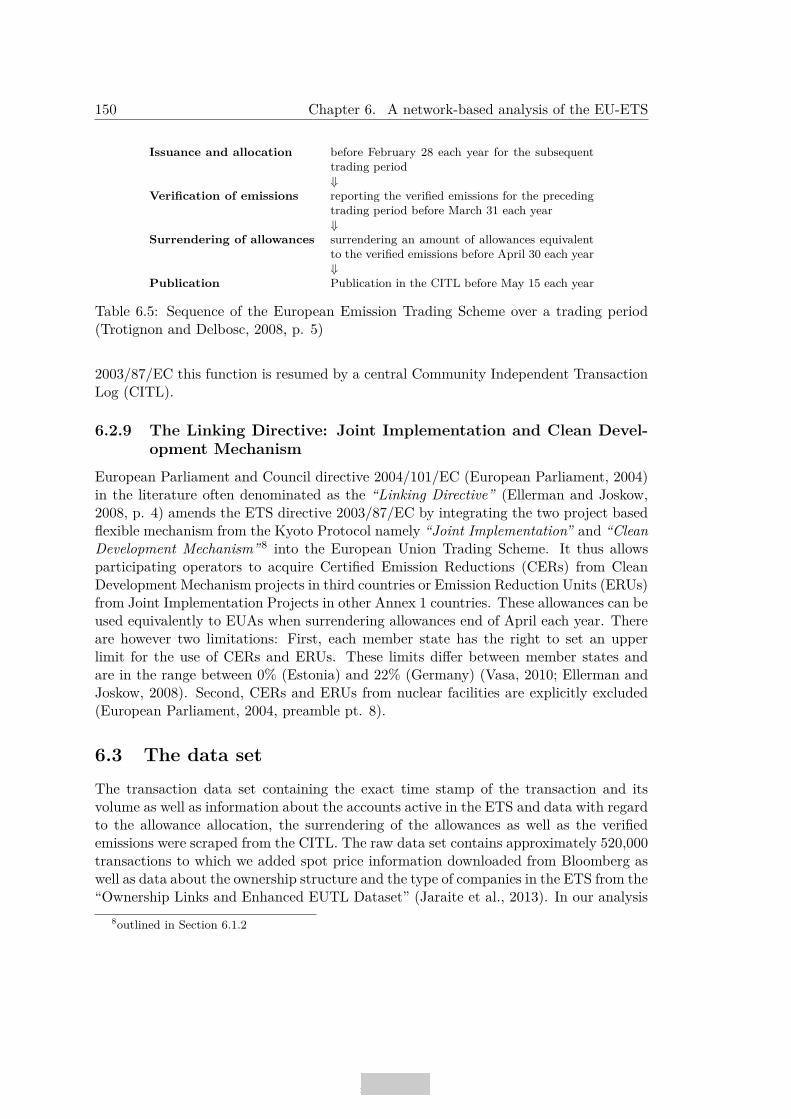
150 Chapter 6. A network-based analysis of the EU-ETS
Issuance and allocation before February 28 each year for the subsequenttrading period⇓
Verification of emissions reporting the verified emissions for the precedingtrading period before March 31 each year⇓
Surrendering of allowances surrendering an amount of allowances equivalentto the verified emissions before April 30 each year⇓
Publication Publication in the CITL before May 15 each year
Table 6.5: Sequence of the European Emission Trading Scheme over a trading period(Trotignon and Delbosc, 2008, p. 5)
2003/87/EC this function is resumed by a central Community Independent TransactionLog (CITL).
6.2.9 The Linking Directive: Joint Implementation and Clean Devel-opment Mechanism
European Parliament and Council directive 2004/101/EC (European Parliament, 2004)in the literature often denominated as the “Linking Directive” (Ellerman and Joskow,2008, p. 4) amends the ETS directive 2003/87/EC by integrating the two project basedflexible mechanism from the Kyoto Protocol namely “Joint Implementation” and “CleanDevelopment Mechanism”8 into the European Union Trading Scheme. It thus allowsparticipating operators to acquire Certified Emission Reductions (CERs) from CleanDevelopment Mechanism projects in third countries or Emission Reduction Units (ERUs)from Joint Implementation Projects in other Annex 1 countries. These allowances can beused equivalently to EUAs when surrendering allowances end of April each year. Thereare however two limitations: First, each member state has the right to set an upperlimit for the use of CERs and ERUs. These limits differ between member states andare in the range between 0% (Estonia) and 22% (Germany) (Vasa, 2010; Ellerman andJoskow, 2008). Second, CERs and ERUs from nuclear facilities are explicitly excluded(European Parliament, 2004, preamble pt. 8).
6.3 The data set
The transaction data set containing the exact time stamp of the transaction and itsvolume as well as information about the accounts active in the ETS and data with regardto the allowance allocation, the surrendering of the allowances as well as the verifiedemissions were scraped from the CITL. The raw data set contains approximately 520,000transactions to which we added spot price information downloaded from Bloomberg aswell as data about the ownership structure and the type of companies in the ETS from the“Ownership Links and Enhanced EUTL Dataset” (Jaraite et al., 2013). In our analysis
8outlined in Section 6.1.2

6.4. Methodology and research questions 151
Figure 6.1: The CO2 trading network [CDM (green),finance (red),foundation (yellow),government (orange), industry (blue)]
we concentrate only on the market movements which are relevant for the price formationof the EUA certificates (transaction types 3-0, 3-21 and 10-0). Transactions connectedto the administration of the ETS as for the allowance issuance, retirement, cancellation,surrender, allocation, and correction were discarded. The remaining 364,810 transactionsare analyzed in what follows.
6.4 Methodology and research questions
A network based analysis of the European Emission market is performed. A networkbased on the transaction data set is therefore constructed. Thereby agents active in theemission market are regarded as vertices. These vertices are connected by directed edgesin the form of transactions from the seller (the source vertex) to the buyer (the targetvertex). The edges are weighted by the volume of EUAs transferred in the respectivetransaction. Figure 6.1 shows a plot of the resulting network graph. The aim is toinvestigate the connection between the network structure and the functioning of themarket. In this context the following research questions are to be addressed:
1. Is the organization of the market reflected in the structure of the network?
2. Which factors are relevant for the matching process on the EU ETS?

152 Chapter 6. A network-based analysis of the EU-ETS
●
●
●
●
●
●
●
●
●
●
●
●
●
●
●
●
●
●
●
●
●
● ●
●
●
●
●
●
●
●
●
●
●
●
●
●
●
●
●
●
●
●
●
●
●
●
●
●
●
●
●
●
●
●
●
●
●
●
●●
●
●
●
●●
●
●
●
●
●
●
●
●
●
●
●
●
●
●
●
●
●
●
●
●
●
●
●●
●
●
●
●
●
●
●
●
●
●
●
●
●
●
●
●
●
●
●
●
●
●
●
●
●
●
●
●
●
●
●
●
●
●
●
●
●
●
●
●
●
●
●
●
●
●
●
●
●
●
●
●●
●
●
●
●
●
●
●
●
●
●
●
●
●
●
●
●
●
●
●
●
●
●
●
●
●
●
●
●
●
●
●
●
●
●
●
●
●
●
●
●
●
●
●
●
●
●
●
●
●
●
●
●
●
●
●●
●
●
●
●
●
●
●
●
●
●
●
●
●
●
●●
●
●
●
●
●
●
●
●
●
●
●
●
●
●
●
●
●
●
●
●
●
●
●
●
●
●
●
●
●
●
●
●
●
●
●
●●
●
●
●
●
●
●
●
●●
●
●
●
●
●
●
●
●
●
●
●
●
●
●
●
●
●
●
●
●
●
●
●
● ●
●
●
●
●
●●
●
●
●
●
●
●
●
●
●
●
●
●
●
● ●
●
●
●
●
●
●
●
●
●
●
●
●
●
●
●
●
●
●
●
●
●
●
●
●
●
●
●
●
●
●
●
●
●
●
●
●
●
●
●
●
●
●
●
●
●
●
●
●
●
●
●
●
●
●
●
●
●●
●
●
●
●
●
● ●
●
●
●
●
●
●
●
●●
●
●
●
●
●
●
●
●
●
●
●
●
●
●
●
●
●
●
●
●
●●
●
●
●
●
●●
●●
●
●
●
●
●
●
●
●
●
●
●
●
●
●
●
●
●
●
●
●
●
●
●
●
●
●
●
●
●
●
●
●
●
●
●
●
●
●
●
●
●
●
●
●
●
●
●
●
●●
●
●
●
●●
●
●
●
●
●
●
●
●
●
●
●
●
●
●
●
●
●
●
●
●
●
●
●
●
●
●
● ●
●
●
●
●●
●
●
●
●
●
●
●
●
●
●
●
●
●
●
●●
●
●
●
●
●
●
●
●
●●
●
●
●
●
●
●
●
●
●
●
●
●
●
●
●
●
●
●
●
●
●
●
●
●●
●
●
●
●
●
●
●
●
●
●
●
●
●
●
●
●
●
●
●
●
●
●●
●
●
●
●
●
●
●
●
●
●
●●
●
●
●
●
●
●
●●
●
●●
●
●
●
●
●
●
●
●●●
●
●
●
●
●
●●
●●
●
●
●
●
●
●
●
●
●
●
●
●
●
●
●
●
●
●
●
●
●
●
●
●
●
●
●
●
●
●
●
●
●
●
●
●
●
●
●
●
●
●
●
●
●
●
●
●
●
●
●
●●●
●●
●
●
●
●
●●
●
●
●
●
●
●
●
●
●
●
●
●
●
●
●
●
●
●
●
●
●
●
●
●
●
●
●
●
●
●
●
●
●
●
●
●
●
●
●
●
●
●
●
●
●
●
●
●
●
●
●
●
●
●
●
●
●
●
●
●
●
●
●
●
●
●
●
●
●
●
●
●
●
●
●
●
●
●
●
●
●
●
●
●
●
●
●
●
●
●
●
●
●
●
●
●
●
●
●
●
●
●
●
●
●
●
●
●
●
●●
●
●
●
●
●
●
●
●
●
●
●
●●
●
●
●
●
●
●
●
●
●
●
●
●
●
●
●
●
●
●
●
●●
●
●
●
●
●
●
●
●
●
●
●
●
●
●
●
●
●
●
●
●
●
●●
●
●
●
●
●
●
●
●
●
●
●
●
●
●
●
●
●
●
●
●
●
●
●
●
●
●
●
●
●
●
●
●
●
●
●
● ●
●
●
●
●
●
●
●
●
●
●
●
●
●
●
●
●
●
●
●
●
●
●
●
●
●
●
●
●
●
●
●
●
●
●●
●
●
●
●
●
●
●
●
●
●
●
●
●
●
●
●
●
●
●
●
●
●
●
●
●
●
●
●●
●
●
●
●
●
●
●
●
●
●
●
●
●
●
●
●
●
●
●
●
●
●
●
●
●
●
●
●
●
●
●
●
●
●
●
●
●
●
●
●
●
●
●
●
●
●
●
●
●
●
●
●
●
●
●
● ●
●
●
●●
●
●
●
●
●
●
●
●●
●
●
●
●
●
●
●●
●
●
●
●
●
●
●
●
●
●
●
●
●
●
●
●
●
●
●
●
●
●
●
●
●
●
●
●
●
●
●
●
●
●
●
●
●
●●
●
●
●
●
●
●
●
● ●
●
●
●
●
●
●
●
●
●
●
●
●●
●
●
●
●
●
●
●
●
●
●
●
●●●
●
●
●
●
●
●
●
●
●
●
●
●
●
●
●
●
●
●
●
●
●
●
●
●
●
●
●
●
●
●
●
●
●
●
●
●
●
●
● ●
●
●
●
●●
●
●
●
●
●
●
●
●
●
●
●
●
●
●
●
●
●
●
●
●
●
●
●
●
●
●
●
●
●
●
●
●
●●
●
●
●
●
●
●
●
●
●
●
●
●
●
●
●
●
●
●
●
●●
●
●
●
●
●
● ●
●
●
●
●
●
●
●
●
●
●
●
●
●
●
●
●
●
●
●
●
●
● ●
●
●
●
●
●
●
●
●
●
●
●
●
●
●
●
●
●
●
●
●
●
●
●
●
●
●
●
●
●
●
●
●
●
●
●
●●
●
●
●
●
●
●
●
●
●
●
●
●
●
●
●
●
●
●
●
●
●
●
●
●
●
●
●
●
●
●
●
●
●
●
●
●
●
●
●
●
●
●
●
●
●
●
●
●
●
●
●
●●
●
●
●
●
●
●
●
●
●
●
●
●
●
●●
●
●
●
●
●
●
●
●
●
●
●
●
●
●
●
●
●
●
●
●
●
●●
●
●
●
●
●
●
●
●
●
●
●
●
●
●●
●
●
●
●
●
●
●
●
●
●
●
● ●
●
●
●
●
●
●
●
●
●
●
●
●
●
●
●
●
●
●
●
●
●
●
●
●
●
●
●●
●
●
●
●
●
●
●
●
●
●
●
●
●
●
●
●
●
●
●
●
●
●
●
●
●
●
●
●
●
●
●
●
●
●
●
●
●
●
●
●
●
●
●
●
●
●
●
●
●
●
●
●
●
●
●
●
●●
●
●
●
●
●●
●
●
●
●
●
●
●
●
● ●
●●
●
●
●
●
●●
●
●●
●
●
●
●
●
●
●
●
●
●
●●
●
●
●●
●
●●
●
●
●
●
●
● ●
●
●
●
●●
●
●
●
●
●
●
●
●
●
●
●
●
●
●
●
●
●
●
●
●
●
●
●
●
●
●
●
●
●
●
●
●
●
●
●
●
● ●
●
●
●
●
●
●
●
●
●
●
●
●
●
●
●
●
●
● ●
●
●
●
●
●
●
●
●
●
●
●
●
●
●
●●
●
●
●
●
●
●
●
●
●
●
●
●
●
●
●
●
●
●
●
●
●
●
●
●
●
●
●
●
●
● ●
●
●
●
●
●
●
●
●
●
●
●
●
●
●
●
●
●
●
●
●
●
●
●
●
●
●
●
●●
●
●
●
●
●
●
●
●
●
●
●
●
●
●
●
●
●●
●
●
●●
●
● ●
●
●
●
●
●
●
●
●
●
●
●●
●
●
●
●
●
●
●
●
●
●●
●
●
●
● ●●
●
●
●
●
●
●
●● ●
●
●
●
●
●
●
●
●
●
●
●●
●●
●
●
●
●
●
●
●
●
●
●●
●
●●
●
●
●
●
●
●
●
●●
●
●
●
●
● ●
●
●
● ●
●●
●
●
●
●
●
● ●
●
●
●
●
●
●
●
●
●
●
●
●
●
●
●
●
●
●
●
●
●
●
●
●
●
●
●
●
●
●
●
●
●
●
●
●
●
●
●
●
●
●
●
●
●
●●
●
●
●
●
●
●
●
●
●
●●
●
●
●
● ●
●
●
●
●
●
●
●●
●
●
●
●
●
●
●
●
●
● ●
●
●
●
●
●
●
●
●
●
●
●●
●
●
●
●
●
●
●
●
●
●
●
●
●
●
●
●
●●
●
●
●
●
●
●
●
●
● ●
●
●
●
●●
●
●
●
●●
●
●
●
●
●
●
●
●
●
●
●
●
●
●
●
●
●
●
●
●
●
●●●
●
●●●●
●
●●
●
●
●
●
●
●●●
●
●●●●●●●●●●
●
●
●
●●
●
●
●●
●
●
●
●
●
● ●
●
●
●
●
●
●
●
●
●
●
●
●
●
●
●
●
●
●
●
●
●
●
●
●
●
●
●
●
●
●
●
●
●
●
●
●
●
●
●
●
●
●
●
●
●
●
●
●
●
●
●
●
●
●
●
●
●
●
●
●
●
●
●
●
●
●●
●
●
●
●
●
●
●●
●
●
●
●
●
●
●
●
●
●
●
●
●
●
●
●●
●
●
●
●
●
●
●
●
●
●
●
●
●
●●
●
●
●
●
●
●
●
●
●
●●
●
●
●
●
●
●
●
●
●
●
●
●
●
●
●
●
●
●
●
●
●
●
●
●
●
●
●
●
●
●
●
●
●
●
●
●
●
●
●
●
●
●
●
●●
●
●
●
●
●
●
●
●
●
●●
●
●
●
●●
●
●
●
●
●
●
●
●
●
●
●
●
●●
●
●
●
●
●
●
●
●
●
●
●●
●
●
●
●
●
●
●
●
●
●
●
●
●
●
●
●
●
●
●
●
●
●
●
●
●
●
●
●
●
●
●●
● ●
●
●
●
●
●
●
●
●
●
●
●
●
●
●
●
●
●
●
●
●
●
●
●
●
●
●
●
●
●
●
●
●
●
●
●
●
●
●
●
●
●
●
●
●
● ●
●
●
●
●
●
●
●
●
●
●
●
●
●
●
●
●
●
●
●
●
●
●
●
●
●
●
●
●
●
●
●
●
●
●
●
●
●
●
●
●
●
●
●
●
●
●
●
●
●
●
●
●
●
●
●
●
●
●
●
●
●
●
●
●
●
●
●
●
●
●
●
●
●
●
●
●
●
●
● ●
●
●
●
●
●
●
●
●
●
●
●
●
●
●
●
●
●
●
●
●
●
●
●
●
●
●
●
●
●
●
●
●
●
●
●
●
●
●
●
●
●
●
●
●
●
●
●
●
●
●
●
●
●
●
●
●
●
●
●
●
●
●
●
●
●
●●
●
●
●
●
●
●
●
●
●
●
●
●
●
●
●
●●
●●
●
●
●
●●
●
●
●
●
●
●●
●
●
●
●
●
●
●
● ●●
●
●
●●●
●
●
●
●
●
●
●
●
●
●
●
●
●
●
●
●
●
●
●
●
●
● ●
●
●
●
●
●
●
●
●
●
●
●
●
●
●
●
●
●
●
●
●
●
●
●
●
●
●
●
●
●
●
●
●
●
●
●
●
●
● ●
●
●
●
●
●●
●
●
●
●
●
●
●
●
●
●
●
●
●
●
●
●
●
●
●
●
●
●
●
●
●
●
●
●
●
●●
●
●
●
●
●
●
●
●
●
●
●●
●
●
●
●
●
●
●
●
●
●
●
●
●
●
●●
●
●
●
●
●
●
●
●
●
●
●
●
●
●
●
●
●
●
●
●●
●
●
●
●
●
●
●●
●
●
●
●
●
● ●
●
●
●
●
●
●
●●●
●
●
●
●
●
●
●
●
●
●
●
●
●
●
●●
●
●●
●
●
●
●
●
●
●
●
●
●●
● ●
●
●
●
●
● ●
●
●
●
●
●
●
●
●
●
● ●
●●
●
●
●
●
●
●
●
●
●
●●
●
●
●
●
●
●
●
●
●
●
●
●
●
●
●
●
●
●
● ●
●
●
●
●
●
●
●
●
●
●
●
●
●
●
●
●
●
●
●
●
●
●
●
●
●
●
●
●
●
●
●
●
●
●
●
●
●
●
●
●
●●
●
●
●
●
●
●●
●
●
●
● ●
●
●
●
●
●
●
● ●● ●
●
●●
●
●
●
●
●● ●
●
●
●
●
●
●
●
●
●
●
●
●
●
●
●
●
●
●
●
●
●
●
●
●●
●
●
●
●
●
●
●
●
●
●
●●
●
●●
●
●
●
●
●
●
●
●
●
● ●
●
●●
● ●
●
●
●
●
●
●●
●
●
●
●
●
● ●
●
●
●
●
●
●
●
●
●
●
●●
●
●
●
●
●
●
●
●
●
●
●
●
●
●
●●
●
●
●
●
●
●
●●
●
●●
●
●
●
●
●
●
●
●
●
●
●
●
●
●
●
●
●
●
●
●
●
●
● ●
●
●
●
●
●●
●
●●
●
●
●
●● ●
●
●
●
●●●
●●
●
●
●
●
●
●
●
●●
●
●
●●
●
●
●
●
●
●
●
●
●
●
●
●
●
●
●
●
●
●
●
●
●
●●
●
●
●
●
●
●
●
●
●
●
●
●
●●
●●
●
●●
●
●
●
●
●
●●
●
●
●
●
●●
●
●
●●●
●
●
●
●
●
●
●
●
●
●
●
●
●
●
●
●
●
●
●
●
●
●●●
●
●
●
●
●●
●●●
●
●
●
●
●
●
●
●
●
●
●
●
●
●
●
●
●
●
●
●
●
●
●
●
●
●
●
●
●
●
●
●
●
●
●
●
●
●
●
●
●●
●
● ●●
●
●
●
●
●
●
●
●
●
●
●
●
●
●
●
●
●
●●
●
●
●
●
●
●
●
●
●
●
●
●
●
●
●
●
●
●
●
●
●
●●
●
●
●
●
●
●
●
●
●
●
●●
●
●
●
●
●
●
●
●
●
●
●
●
●
●
●
●
●
●
●
●
●
●
●
●
●
●
●
●
●
●
●
●
●● ●
●
●
●
●
●
●
●
●
●
●
●
●
●
●
●
●
●
●
●
●
●
●
●
●
●
●
●
●
●
●
●
●
●
●
●
●
●
●
●
●
●
●
●
●
●
●
●
●
●
●
●
●
●
●●
●
●
●
●
●
●
●
●
●
●
●
●
●
●
●
●
●
●
●
●
●
●
●
●
●
●●
●
●
●
●
●
●
●
●
●
●
● ●
●
●
●
●
●
●
●
●
●
●
●
●
●
●
●
●
●
●
●
●
●
●
●
●
●
●
●
●
●
●
● ●
●
●
●
●
●
●
●
●
●
●
●
●
●
●
●
●
●
●
●
●●
●
●
●
●
●
●
●
●
●
●
●
●
●
●
●
●
●
●
●
●
● ●
●
● ●
●
●
●
●
●
●
●
●
●
●
●
●
●
●
●●
●
●
●
●
●
●
●
● ●
●
● ●
●
●
●
●
●
●
●
●
●
●
●
●
●
●
●
●
●
●
●
●
●
●
●
●
●
●
●
●
●●
●
●
●
●
●
●
●
●
●
●
●
●
●
●
●
●
●
● ●
●
●
●
●
●
●
●
●●
●
●●
●
●
●
●
●
●
●
●
●
●
●
●
●
●
●
●●●
●
●●
●
●
● ●
●
●
●
●
●●
●
●
●
●
●
● ●●
●
●
● ●
●
●
●
●
●
●
●
●
●
●
●
●
●
●
●
●
●
● ●●
●
●
●
●●
●
●
●
●
●
●
●
●
●
●
●
●
●
●
●
●
●
●
●
●
●
●
●
●
●
●
●
●
● ●
●
●
●
●
●
●
●
●●●
●
●
●
●
●
●●●
●
●
●
●
●
●
●
●
● ●
●
●
●
●
●
●
●
●
●
●
●
●
●
●
●
●
●
●
●
●
●●
●
● ●
●
●
●
●
●
●
●
●●
●
●
●●
●
● ●
●
●
●
●
● ●●●
●
●
●
●
●
●●●
●
●● ● ●
●
●●
●
●●
●
●
●
● ●
●
●
●
●
●
●
●
●
●
●
●
●
●
●
●
●
●
●●
●
● ●●
●
● ●
●
●
●
●
●
●
● ●●
●
●
●
●
●
●
●
●
●
●
●●
●
●
●●●●
●●
●
●
● ●
●
●
●
●
●
●●
●
●
●
● ●
●
●
●
●
●
●
●
●
●
●
●
●
●
●
●
●
●
●
●
●
●
●
●
●
●
●
●
●
●
●
●
●
●
●●
●
●
●
●
●
●
●
●
●
●
●
●
●
●
●
●
●
●
●
●
●
●
●
●
●
●
●●
●
●
●
●
●
●
●
●●
●
●
●●
●
●
●
●
●
●
●
●
●
●
●
●
●
●
●
●
●
●
●
●
●
●
●
●
●
●
●
●●●●●●
●
●
●
●
●
●
●
●
●
●
●
●
● ●●
●
●
●
●●
●
● ●
●
●
●
●●
●
●
●
●●
●
●
●
●
●
●●
●
●
●
●●
●
●
●
●
●
●
●
●
●●
●
●●
●
●
●
●
●●
●●
●
●
●
●
●●
●
●
●●● ●
●
●●
●
●
●
●
●
●
●
●
●
●
●
●
●
●
●
● ●
●
●
●
● ●
●
●
●
●
●
●
●
●
●
●●
● ●
●
●
●
●
●
●
●●
●
●
●
●
●
●●
●
●
●
●
●
●
●
●
●
●
●
●
●●●
●
●
●
●
●
●
●
●
●
●
●●
●
●
●
●
●●
●
●
●
●
●
●
●
●
●
●
●●
●
●
●
●
●
●
●
●
●●
●
●
●
●
●
●
●
●
●
●●
●
●
●
●
●
●
●
●
●
●●
●
●
●
●
●
●
●
●
●
●
●
●
●
●
●
●●
●
●
●
●
●
●
●●
●
●
●
●
●●
●
●
●
●
●
●
●
●
●
●
●
●
● ●
●
●
●●
●
● ●
●
●
●
●
●
●
●
●
●
●
● ●●●
●● ●
●
●
●
●
●
●
● ●
●
●
●
●●
●●
●
●
●
●
●
●
●
●
●
●
●
●
●
●
●
●
●
●
●
●●●
●
●●●●
●●
●●●
●
●
●●
●
●
●
●
●
●
●
●
●
●
●
●
●
●
● ●
●
●
●●
●
●
●
●
●
●
●
●
●
●
●
●
●
●●
●
●●
●●
●
●
●
●
●●
●
●●
●
●
●●
●
●
●
●
●
●●●●
●
●
●
●
●
●
●
●
●
● ●
●
●
●
●
●
●●●
●
●
●
●
●
●
● ●
●●●
●
●●●
●
●● ●
●
●
●
●
●
●
●
●● ●●
●
●
●
●
●
●
● ●
●●
●
●
●
●
●
●
●
●
●
●
● ●
●
●
●●
●
●
●
●
●
●
●
●
●
●
●
●
●●
●
●●
●
●
●●
●●
●
●
●●
●
●●●
●
●
●
●
●●
●
●
●
●
●
●●
●
●
●●●●●●
●
●
●●●
●
●
●
●●●
●
●
●
●●
●
●
●
●
●
●
●
●
●
●
●
●
●
●
●
●
●
●
●
●
●
●
●
●
●
●
●
●
●
●●
●●
●
●
●
●
●
●
●
●
●
●●
●●●
●
●
●
●
●
●
●●
●
●
●
●●
●
●
●
●
●
●
●
●
●
●
●●●
●
●
●
●
●
●
●
●
●●● ●●
●●●
●
●●●●●●●●●●●●●● ●●●●●●●● ●●
●
●
●●●
●
●●●●●
●
● ●●●●
●●
●
●●
●
●●
●
●
●●
●
●●
●
●
●
●
●
●●●●●●
●
●●
●
●●●●
●
●
●
●
●
●
●●●● ●●
●
●●●●●●
●
●
●
●●●●●●
●
●●●●●
●●
●●●● ●●●●
●
●●
●
●●
●
●●
●
●●●●
●
●
● ●●●●
●
●
●
●
●
●
●●
●
●
●
●
●●●●●
●
●
●
●●
●
●●
●●
●
●
●●
●
●
●●●●
●
●●
●
●●●●●●●●
●●●●
●
●
●
●●●●●●
●
●
●
●
●●●●●●
●
●●●●●●●●
●
●
●●
●
●●
●
●
●●●●
●
●
●
●
●
●
●
●
●
●
●
●
●
●
●
●
●
●
●
●
●
●●
●
●
●
●
●
●
●
●
●
●
●
●
●
●
●
●
●
●
●
●
●
●
●
●
●
●
●
●
●
●
●
●
●
●
●
●●
●
●
●
●●
●
●
●
●
●
●
●
●
●
●
●
●
●
●
●
●
●
●
●
●
●
●
●●
●
●
●
●
●
●
●
●
●
●
●
●
●
●
●
●
●
●
●
●
●
●
●
●
●
●
●
●
●
●
●
●
●
●
●
●
●
●
●
●
●
●
●
●
●
●
●
●
●
●
●
●
●●
●
●
●
●
●
●
●
●
●
●
●
●
●
●
●
●
●
●
●
●
●
●
●
●
●
●
●
●
●
●
●
●
●
●
●
●
●
●
●
●
●
●
●
●
●
●
●
●
●
●
●
●
●
●
●●
●
●
●
●
●
●
●
●
●
●
●
●
●
●
●●
●
●
●
●
●
●
●
●
●
●
●
●
●
●
●
●
●
●
●
●
●
●
●
●
●
●
●
●
●
●
●
●
●
●
●
●●
●
●
●
●
●
●
●
●●
●
●
●
●
●
●
●
●
●
●
●
●
●
●
●
●
●
●
●
●
●
●
●
●●
●
●
●
●
●●
●
●
●
●
●
●
●
●
●
●●
●
●
●
●●
●
●
●
●
●
●
●
●
●
●
●
●
●
●
●
●
●
●
●
●
●
●
●
●
●
●
●
●
●
●
●
●
●
●
●
●
●
●
●
●
●
●
●
●
●
●
●
●
●
●
●
●
●
●
●
●
●
●
●
●●
●
●
●
●
●
●
●●
●
●
●
●
●
●
●
● ●
●
●
●
●
●
●
●
●
●
●
●
●
●
●
●
●
●
●
●
●
● ●
●
●
●
●
● ●
●●
●
●
●
●
●
●
●
●
●
●
●
●
●
●
●
●
●
●
●
●
●
●
●
●
●
●
●
●
●
●
●
●
●
●
●
●
●
●
●
●
●
●
●
●
●
●
●
●
●
●●
●
●
●
●●
●
●
●
●
●
●
●
●
●
●
●
●
●
●
●
●
●
●
●
●
●
●
●
●
●
●
●
● ●
●
●
●
● ●
●
●
●
●
●
●
●
●
●
●
●
●
●
●
●
●●
●
●
●
●
●
●
●
●
●●
●
●
●
●
●
●
●
●
●
●
●
●
●
●
●
●
●
●
●
●
●
●
●
●●
●
●
●
●
●
●
●
●
●
●
●
●
●
●
●
●
●
●
●
●
●
●
●
●
●
●
●
●
●
●
●
●
●
●
●
●●
●
●
●
●
●
●
● ●
●
●●
●
●
●
●
●
●
●
●●●
●
●
●
●
●
● ●
● ●
●
●
●
●
●
●
●
●
●
●
●
●
●
●
●
●
●
●
●
●
●
●
●
●
●
●
●
●
●
●
●
●
●
●
●
●
●
●
●
●
●
●
●
●
●
●
●
●
●
●
●
●
●
●●●
● ●
●
●
●
●
●●
●
●
●
●
●
●
●
●
●
●
●
●
●
●
●
●
●
●
●
●
●
●
●
●
●
●
●
●
●
●
●
●
●
●
●
●
●
●
●
●
●
●
●
●
●
●
●
●
●
●
●
●
●
●
●
●
●
●
●
●
●
●
●
●
●
●
●
●
●
●
●
●
●
●
●
●
●
●
●
●
●
●
●
●
●
●
●
●
●
●
●
●
●
●
●
●
●
●
●
●
●
●
●
●
●
●
●
●
●
●
●
●
● ●
●
●
●
●
●
●
●
●
●
●
●
●●
●
●
●
●
●
●
●
●
●
●
●
●
●
●
●
●
●
●
●
●●
●
●
●
●
●
●
●
●
●
●
●
●
●
●
●
●
●
●
●
●
●
●●
●
●
●
●
●
●
●
●
●
●
●
●
●
●
●
●
●●
●
●
●
●
●
●
●
●
●
●
●
●
●
●
●
●
●
●
●
● ●
●
●
●
●
●
●
●
●
●
●
●
●
●
●
●
●
●
●
●
●
●
●
●
●
●
●
●
●
●
●
●
●
●
●
●●
●
●
●
●
●
●
●
●
●
●
●
●
●
●
●
●
●
●
●
●
●
●
●
●
●
●
●
●
●●
●
●
●
●
●
●
●
●
●
●
●
●
●
●
●
●
●
●
●
●
●
●
●
●
●
●
●
●
●
●
●
●
●
●
●
●
●
●
●
●
●
●
●
●
●
●
●
●
●
●
●
●
●
●
●
●●
●
●
●●
●
●
●
●
●
●
●
● ●
●
●
●
●
●
●
●●
●
●
●
●
●
●
●
●
●
●
●
●
●
●
●
●
●
●
●
●
●
●
●
●
●
●
●
●
●
●
●
●
●
●
●
●
●
●●
●
●
●
●
●
●
●
●●
●
●
●
●
●
●
●
●
●
●
●
●
●●
●
●
●
●
●
●
●
●
●
●
●
●
●● ●
●
●
●
●
●
●
●
●
●
●
●
●
●
●
●
●
●
●
●
●
●
●
●
●
●
●
●
●
●
●
●
●
●
●
●
●
●
●
●●
●
●
●
●
● ●
●
●
●
●
●
●
●
●
●
●
●
●
●
●
●
●
●
●
●
●
●
●
●
●
●
●
●
●
●
●
●
●
●
●
●
●●
●
●
●
●
●
●
●
●
●
●
●
●
●
●
●
●
● ●
●
●
●●
●
●
●
●
●
● ●
●
●
●
●
●
●
●
●
●
●
●
●
●
●
●
●
●
●
●
●
●
●●
●
●
●
●
●
●
●
●
●
●
●
●
●
●
●
●
●
●
●
●
●
●
●
●
●
●
●
●
●
●
●
●
●
●
●
●
●●
●
●
●
●
●
●
●
●
●
●
●
●
●
●
●
●
●
●
●
●
●
●
●
●
●
●
●
●
●
●
●
●
●
●
●
●
●
●
●
●
●
●
●
●
●
●
●
●
●
●
●●
●
●●
●
●
●
●
●
●
●
●
●
●
●
●
●
●●
●
●
●
●
●
●
●
●
●
●
●
●
●
●
●
●
●
●
●
●
●
●
●
●●
●
●
●
●
●
●
●
●
●
●
●
●
●
●●
●
●
●
●
●
●
●
●
●
●
●
● ●
●
●
●
●
●
●
●
●
●
●
●
●
●
●
●
●
●
●
●
●
●
●
●
●
●
●
●
●
●
●
●
●
●
●
●
●
●
●
●
●
●
●●
●
●
●
●
●
●
●
●
●
●
●
●
●
●
●
●
●
●
●
●
●
●
●
●
●
●
●
●
●
●
●
●
●
●
●
●
●
●
●
●
●
●
●
●
●
●
●
● ●
●
●
●
●
●
● ●
●
●
●
●
●
●
●
●
●●
●●
●
●
●
●
●●
●
● ●
●
●
●
●
●
●
●
●
●
●
●
●
● ●
●
●
●
●●
●
●●
●
●
●
●
●
●
●
●
●
●
●
●
●
●
●
●● ●
●
●
●
●
●
●
●
●
●
●
●
●
●
●
●
●
●
●
●
●
●
●
●
●
●
●
●
●
●
●
●
●
●
●
●
●
●
●●
●
●
●
●
●
●
●
●
●
●
●
●
●
●
●
●
●
●
●
●
●
●
●
●
●
●
●
●
●
●
●
●
●
●
●
●●
●
●
●
●
●
●
●
●
●
●
●
●
●
●
●
●
●
●
●
●
●
●
●
●
●
●
●
●
●
●●
●
●
●
●
●
●
●
●
●●
●
● ●
●
●
●
●
●
●
●
●
●
●
●
●
●
●
●
●
●
●
●●
●
●
●
●
●
●
●
●
●
●
●
●
●
● ●
●
●
●●
●
●
●●
●
●●
●
●
●
●
●
●
●
●
●
●
●
●●
●
●
●
●
●
●
●
●
●
●●●
●
●
●
●●●
●
●
●
●
●
●
●●●
●
●
●
●
●
●
●
●
●
●
●●
●●
●
●
●
●
●
●
●
●
●
● ●
●
● ●
●
●
●
●
●
●
●
●●
●
●
●
●
● ●
●
●
●●
●●
●
●
●
●
●
● ●
●
●
●
●
●
●
●
●
●
●
●
●
●
●
●
●
●
●
●
●
●
●
●
●
●
●
●
●
●
●
●
●
●
●
●
●
●
●
●
●
●
●
●
●
●
●●
●
●
●
●
●
●
●
●
●
●●
●
●
●
●●
●
●
●
●
●
●
● ●
●
●
●
●
●
●
●
●●●
●
●
●
●●
●
●
●
●
●●
●
●
●
●
●
●
●
●●
●
●
●
●
●
●
●
●
●
●
●
●
●
●
●
●
● ●
●
●
●
●
●
●
●
●
●
● ●
●
●
●
●
●●
●
●
●
●●
●
●
●
●
●
●
●
●
●
●
●
●
●
●
●
●
●
●
●
●
●
●
●●●
●
●●●●
●
● ●
●
●
●
●
●
●●●
●
●●●●●●●●● ●
●
●
●
●●
●
●
● ●
●
●
●●
●
●
●●
●
●
●
●
●
●
●
●
●
●
●
●
●
●
●
●
●
●
●
●
●
●
●
●
●
●
●
●
●
●
●
●
●
●
●
●
●
●
●
●
●
●
●
●
●
●
●
●
●
●
●
●
●
●
●
●
●
●
●
●
●
●
●
●
●
●
●
●
●
●●
●
● ●
●
●
●
●
●
●
● ●
●
●
●
●
●
●
●
●
●
●
●
●
●
●
●
●
●●●
● ●
●
●
●
●
●
●
●
●
●
●
●
●
●
●●
●
●
●
●
●
●
●
●
●
●
●●
●
●
●
●
●
●
●
●
●
●
●
●
●
●
●
●
●
●
●
●
●
●
●
●
●
●
●
●
●
●
●
●
●
●
●
●
●
●
●
●
●
●
●
● ●
●
●
●
●
●
●
●
●
●
●●
●
●
●
●●
●
●
●
●
●
●
●
●
●
●
●
●
●●
●
●
●
●
●
●
●
●
●
●
●
●●
●
●
●
●
●
●
●
●
●
●
●
●
●
●
●
●
●
●
●
●
●
●
●
●
●
●
●
●
●
●
●
●
●●
●●
●
●
●
●
●
●
●
●
●
●
●
●
●
●
●
●
●
●
●
●
●
●
●
●
●
●
●
●
●
●
●
●
●
●
●
●
●
●
●
●
●
●
●
●
● ●
●
●
●
●
●
●
●
●
●
●
●
●
●
●
●
●
●
●
●
●
●
●
●
●
●
●
●
●
●
●
●
●
●
●
●
●
●
●
●
●
●
●
●
●
●
●
●
●
●
●
●
●
●
●
●
●
●
●
●
●
●
●
●
●
●
●
●
●
●
●
●
●
●
●
●
●
●
●
●
●
●
●
●
●
●
● ●
●
●
●
●
●
●
●
●
●
●
●
●
●
●
●
●
●
●
●
●
●
●
●
●
●
●
●
●
●
●
●
●
●
●
●
●
●
●
●
●
●
●
●
●
●
●
●
●
●
●
●
●
●
●
●
●
●
●
●
●
●
●
●
●
●
●●
●
●
●
●
●
●
●
●
●
●
●
●
●
●
●
●●
●●
●
●
●
●●
●
●
●
●
●
●●
●
●
●
●
●
●
●
●
●●●
●
●
● ●●
●
●
●
●
●
●
●
●
●
●
●
●
●
●
●
●
●
●
●
●
●
●
●●
●
●
●
●
●
●
●
●
●
●
●
●
●
●
●
●
●
●
●
●
●
●
●
●
●
●
●
●
●
●
●
●
●
●
●
●
●
●
●
●
●
●●
●
●
●
●
●
●●
●
●
●
●
●
●
●
●
●
●
●
●
●
●
●
●
●
●
●●
●
●
●
●
●
●
●
●
●
●
●
●●
●
●
●
●
●
●
●
●
●
●
● ●●●
●
●
●
●
●
●
●
●
●
●
●
●
●
●
●●
●
●
●
●
●
●
●
●
●
●
●
●
●
●
●
●
●
●
●
●
●●
●
●
●
●
●
●
●
● ●
●
●
●
●
●
●●
●
●
●
●
●
●
●●●
●
●
●
●
●
●
●
●
●
●
●
●
●
●
●
● ●
●
●●
●
●
●
●
●
●
●
●
●
●●
●●
●
●
●
●
●●
●
●
●
●
●
●
●
●
●
●
●
●●
●●
●
●
●
●
●
●
●
●
●
● ●
● ●
●
●
●
●
●
●
●
●
●
●
●
●
●
●
●
●
●
●
●
●●
●
●
●
●
●
●
●
●
●
●
●
●
●
●
●
●
●
●
●
●
●
●
●
●
●
●
●
●
●
●
●
●
●
●
●
●
●
●
●
●
●●
●
●
●
●
●
●●
●
●
●
●
●●
●
●
●
●
●
●
●●●●
●
●●
●
●
●
●
● ●●
●
●●●
●
●
●
●
●
●
●
●
●
●
●
●
●
●
●
●
●
●
●
●
●
●
●
●
●●
●
●
●
●
●
●
●
●
●
●
●●
●
●●
●
●
●
●
●
●
●
●
●
●●
●
●
●
●
●●
● ●
●
●
●
●
●
●●
●
●
●
●
●
●●
●
●
●
●
●
●
●
●
●
●
● ●
●
●
●
●
●
●
●
●
●
●
●
●
●
●
●
● ●
●
●
●
●●
●
●
●●
●
● ●
●
●●
●
●
●
●
●
●
●
●
●
●
●
●
●
●
●
●
●
●
●
●
●
● ●
●
●
●
●
●●
●
●●
●
●
●
●●●
●
●
●
●● ●
●
●●
●
●
●
●
●
●
●
●●
●
●
● ●
●
●
●
●
●
●
●
●
●
●
●
●
●
●
●
●
●
●
●
●
●
●●
●
●
●
●
●
●
●
●
●
●
●
●
●
●
●●
● ●
●
●●
●
●
●
●
●
●●
●
●
●
●
●●
●
●
●● ●
●
●
●
●
●
●
●
●
●
●
●
●
●
●
●
●
●
●
●
●
●
●●●
●
●
●
●
●●
●●●
●
●
●
●
●
●
●
●
●
●
●
●
●
●
●
●
●
●
●
●
●
●
●
●
●
●
●
●
●
●
●
●
●
●
●
●
●
●
●
●
●●
●
●● ●
●
●
●
●
●
●
●
●
●
●
●
●
●
●
●
●
●
●
●●
●
●
●
●
●
●
●
●
●
●
●
●
●
●
●
●
●
●
●
●
●
●
●
●●
●
●
●
●
●
●
●
●
●
●
● ●●
●
●
●
●
●
●
●
●
●
●
●
●
●
●
●
●
●
●
●
●
●
●
●
●
●
●
●
●
●
●
●
●
●
● ●
●
●
●
●
●
●
●
●
●
●
●
●
●
●
●
●
●
●
●
●
●
●
●
●
●
●
●
●
●
●
●
●
●
●
●
●
●
●
● ●
●
●
●
●
●
●
●
●
●
●
●
●
●
●
●
●
●
●●
●
●
●
●
●
●
●●
●
●
●
●
●
●
●
●
●
●
●
●
●
●
●
●
●
●
●
●●
●
●
●
●
●
●
●
●
●
●
●●
●
●
●
●
●
●
●
●
●
●
●
●
●
●
●
●
●
●
●
●
●
●
●
●
●
●
●
●
●
●
●
● ●
●
●
●
●
●
●
●
●
●
●
●
●
●
●
●
●
●
●
●
●
●
●●
●
●
●
●
●
●
●
●
●
●
●
●
●
●
●
●
●
●
●
●
●
●
● ●
●
●●
●
●
●
●
●
●
●
●
●
●
●
●
●
●
●●
●
●
●
●
●
●
●
●●
●●
●
●●
●
●
●
●
●
●
●
●
●
●
●
●
●
●
●
●
●
●
●
●
●
●
●
●
●
●
●
●
●
●●
●
●
●
●
●
●
●
●
●
●
●
●
●
●
●
●
●
●
●●
●
●
●
●
●
●
●
●●
●
● ●
●
●
●
●
●
●
●
●
●
●
●
●
●
●
●
●●●
●
●●
●
●
●●
●
●
●
●
●●
●
●
●
●
●
●
●● ●
●
●
●
●
●
●
●
●
●
●
●
●
●
●
●
●
●
●
●
●
●
●
●● ●
●
●
●
●●
●
●
●
●
●
●
●
●
●
●
●
●
●
●
●
●
●
●
●
●
●
●
●
●
●
●
●
●
●
●
●●
●
●
●
●
●
●
●
● ●●
●
●
●
●
●
● ●●
●
●
●
●
●
●
●
●
●●
●
●
●
●
●
●
●
●
●
●
●
●
●
●
●
●
●
●
●
●
●●
●
●●
●
●
●
●
●
●
●
●●
●
●
●●
●
●●
●
●
●
●
●●● ●
●
●
●
●
●
●●●
●
●●●●
●
●●
●
● ●
●
●
●
●● ●
●
●
●
●
●
●
●
●
●
●
●
●
●
●
●
●
●
●●
●
●●●
●
●●
●
●
●
●
●
●
●●●
●
●
●
●
●
●
●
●
●
●
●●
●
●
●
●
●
●●●●
●●
●
●
●
●●
●
●
●
●
●
●●
●
●
●
●●
●
●
●
●
●
●
●
●
●
●
●
●
●
●
●
●
●
●
●
●
●
●
●
●
●
●
●
●
●
●
●
●
●
●
●●
●
●
●
●
●
●
●
●
●
●
●
●
●
●
●
●
●
●
●
●
●
●
●
●
●
●
●
●●
●
●
●
●
●
●
●
● ●
●
●
●●
●
●
●
●
●
●
●
●
●
●
●
●
●
●
●
●
●
●
●
●
●
●
●
●
●
●
●
●●●●●●
●
●
●
●
●
●
●
●
●
●
●
●
●●●
●
●
●
●●
●
●●
●
●
●
●●
●
●
●
●
● ●
●
●
●
●
●
●●
●
●
●
●●
●
●
●
●
●
●
●
●
●●
●
●●
●
●
●
●
●●
●●
●
●
●
●
●●
●
●
●●●●
●
●
●●
●
●
●
●
●
●
●
●
●
●
●
●
●
●
●
●
●●
●
●
●
●●
●
●
●
●
●
●
●
●
●
●●
●●
●
●
●
●
●
●
●●
●
●
●
●
●
●●
●
●
●
●
●
●
●
●
●●
●
●
●
●●●
●
●
●
●
●
●
●
●
●
●
●●
●
●
●
●
● ●
●
●
●
●
●
●
●
●
●
●
●●
●
●
●
●
●
●
●
●
●
●
●
●
●
●
●
●
●
●
●
●
● ●
●●
●
●
●
●
●
●
●
●
●
●●
●
●
●
● ●
●
●
●
●
●
●
●
●
●
●
●
●●
●
●
●
●
●
●
●●
●
●●
●
●
●
●
●
●
●
●
●
●
●
●
●
●
●
●
●
●
●
●●
●
●
● ●●
●
●●
●
●
●
●
●
●
●
●
●
●
●
●● ●●●
● ●●
●
●
●
●
●
●
●●
●
●
●
●●
●●
●
●
●
●
●
●
● ●
●
●
●
●
●
●
●
●
●
● ●
●
●
●
●●●
●●
●●● ●
●●
●●●
●
●
● ●
●
●
●
●
●
●
●
●
●
●
●
●
●
● ●
●
●
●●
●
●
●
●
●
●
●
●
●
●
●
●
●
●
●
●
●
●
●
● ●
●
●●
●●
●
●
●
●
●●
●
●●
●
●
●●
●
●
●
●
●
● ●●●
●
●
●
●
●
●
●
●
●
●●
●
●
●
●
●
●●●
●
●
●
●
●
●
● ●
●●●
●
●●●
●
● ●●
●
●
●
●
●
●
●
●●●●
●
●
●
●
●
●
●●
●●
●
●
●
●
●
●
●
●
●
●
●●
●
●
●●
●
●
●
● ●
●
●
●
●
●
●
●
●
●
●
●●
●
●●
●
●
●●
●●
●
●
● ●●
●
●●●
●
●
●
●
●●
●
●
●
●
●
●●
●
●
●●●●●●
●
●
●●●
●
●
●
●● ●
●
●
●
●●
●
●
●
●
●
●
●
●
●
●
●
●
●
●
●
●
●
●
●
●
●
●
●
●
●
●
●
●
●
●
●●
●●
●
●
●
●
●
●
●
●
●
●●
●●●
●
●
●
●
●
●
● ●
●
●
●
●
●●
●
1 2 5 10 20 50 100 200 500
5e−
04
5e−
03
5e−
02
5e−
01
Degree
Clu
ste
ring C
oeffic
ient
Figure 6.2: In-/Out-Degree vs. Cliquishness (in-degree: blue; out-degree: red)
3. Is the network structure supporting the idea of emission markets to exploit differ-ences in marginal abatement costs?
4. Does the position of an agent within the network have an implication for its abilityto create revenues out of a trade?
6.5 The Network structure of the European Emission mar-kets
Along Li and Schürhoff (2014) some tests with regard to the market structure wereconducted. Figure 6.2 plots the in- and out-degrees9 vs. the cliquishness10 of agents.The downward sloping cloud implies a hierarchy in the market with a strong core ofhighly connected nodes and clusters of nodes on the periphery. This phenomenon canalso be observed in the plot of the emission market network in Figure 6.1.
The core periphery structure of the trading network is also observable when lookingat the degree distribution directly (see Figure 6.3): The distributions of the in-, out- andtotal-degrees follow a power law i.e. there are agents whose in-, out- or total degrees
9The in- and out-degrees of each agent: this means the active and passive connectedness of agents.10Be the k-core of graph a maximal subgraph in which each vertex has at least degree k. The cliqishness
or coreness of a vertex is then k if it belongs to the k-core but not to the (k+1)-core (Seidman, 1983).

6.5. The Network structure of the European Emission markets 153
●
●
●
●
●
●
●
●
●
●
●
●
●
●
●
●
●
●
●
●
●
●●
●
●●
●
●
●●
●●
●
● ●
●●
● ●●
● ●●●●●●
●●●
●●●●
●●●
●●
●●●
●●
●●●
●●
●●
●
●●●●
●●●●●●●
●●
●●●●
●●●●●●●
●●●
●●●
●●●●
●●
●●
●
●
●●
●
●●●
●●
●●
●●●●●●
●●●
●●●●
●●●●
●●●●●●●●●●●●●●●●
●●●●●
●●●●●●●●
●
●●●●●
●●●●●●●●●●●●●●●●●●●●●●●●●●●●●●
●●●●●●●●●●
●●●●●●●●●●●●●●●
●●●
●●●●●●●●●●●●●●●●●●●●●●●●●●●●●●●●●●●●●●●●●●●●●●●●●●●●●●●●●●●●●●●●●●●●●●●●●●●●●●●●●
●●●●●●●
●●●●●●●●●●●●●●●●●●●●●●●●●●●●●●●●●●●●●●●●●●●●●●●●●●●●●●●●●●●●●●●●●●●●●●●●●●●●●●●●●●●●●●●●●●●●●●●●●●●●●●●●●●●●●●●●●●●●●●●●●●●●●●●●●●●●●●●●●●●●●●●●●●●●●●●●●●●●●●●●●●●●●●●●●●●●●●●●●●●●●●●●●●●●●●●●●●●●●●●●●●●●●●●●●●●●●●●●●●●●●●●●●●●●●●●●●●●●●●●●●●●●●●●●●●●●●●●●●●●●●●●●●●●●●●●●●●●●●●●●●●●●●●●●●●●●●●●●●●●●●●●●●●●●●●●●●●●●●●●●●●●●●●●●●●●●●●●●●●●●●●●●●●●●●●●●●●●●●●●●●●●●●●●
1 2 5 10 20 50 100 200 500
1e−
04
1e−
03
1e−
02
1e−
01
1e+
00
Indegree
Cum
ula
tive
Fre
quency
●
●
●
●
●
●
●
●
●
●
●
●
●
●
●
●
●
●
●
●
●
●
●●
●
●●
●●
● ●● ●
●
●● ●
●
●
●
●●
●
●●
●●
●●●
●●●●●●
●●
●●
●●
●●
●●
●
●●●●●
●●●●●●
●●●
●
●●●●●●●●●●●●●
●●●●●
●●●●●●
●
●●
●●●●●
●●●●●●●
●●●●
●
●●●●
●●
●
●●●●●●●●●●●●●●●●●●●●●
●●
●
●●●
●
●●●●●●●●●●●●
●●●●●
●●●●●●●●●●●●●●●●●●●●●●
●
●●●●●●●●●●●●●●●●●●●●●●●●●●●●●●●
●
●●●●●●●●●●●●●●●●●●●●●●●●●●●●●●●●●
●●●●●●●●●●●●●●●●
●●●●●●●●●●●●●●●●●●●●●●●●●●●●●●●●●●●●●●●●●●●●●●●●●●●●●●●●●●●●●●●●●●●●●●●●●●●●●●●●●●●●●●●●●●●●●●●●●●●●●●●●●●●●●●●●●●●●●●●●●●●●●●●●●●●●●●●●●●●●●●●●●●●●●●●●●●●●●●●●●●●●●●●●●●●●●●●●●●●●●●●●●●●●●●●●●●●●●●●●●●●●●●●●●●●●●●●●●●●●●●●●●●●●●●●●●●●●●●●●●●●●●●●●●●●●●●●●●●●●●●●●●●●●●●●●●●●●●●●●●●
●●●●●●●●●●●●●●●●●●●●●●●●●●●●●●●●●●●●●●●●●●●●●●●●●●●●●●●●●●●●●●●●●●●●●●●●●●●●●●●●●●●●●●●●●●●●●●●●●●●●●●●●●●●●●●●●●●●●●●●●●●●●●●●●●●●●●●●●●●●●●●●●●●●●●●●●●●●●●●●●●
1 2 5 10 20 50 100 200 500
1e−
04
1e−
03
1e−
02
1e−
01
1e+
00
Outdegree
Cum
ula
tive
Fre
quency
● ●
●
●
●
●
●
●
●
●
●
●
●
●
●
●
●
●
●
●
●
●
●
●
●
●
●
●
●
●
●
●
●
●
●
●
●●
●●
●●
●
●●
●●
●
●●●●●
●●●●●●●
●●●
●●●●●
●●●●●●
●●●●●●●●●●●●●●
●●●●●●●●
●●●●●●
●
●●●●
●●●●●●●●●●●●●●●●
●●●
●●●●●●
●●●●●●●●●●●●●●●●●
●
●●●●●●●●●
●●●●●●●●●●●●
●●●●●●
●●●●●●●
●●●●●●●
●●●●●●●●●
●●
●●●●●
●●
●●●●●●●●●●
●●●●●●
●●
●●●●●●●●●●●●
●●●●●●●●●●●●●●●●●●●●
●
●
●●●●●●●
●●
●●●●●●●●●●●●●●●●●●●●●●●
●●●●
●●●●●●●●●●●●●●●●●●●●●●
●●●●●●●●
●●●●●●●●●●●●●●●●●●●●●●●●●●●●●●●●●●
●●
●●●●●●●
●●●●●●●●●●●
●●●●●●●●●●●●●●●●●●●●●●●●●●●●●●●●●●●●●●●●●●●●●●●●●●●●●●●●●●●●●●●●●●●●●●●●●●●●●●●●●●●●●●●●●●●●●●●●●●●●●●●●●●●●●●●●●●●●●●●●●●●●●●●●●●●
●●●●●●●●●●●●●●●●●●●●●●●●●●●●●●●●●●●●●●●●
●●●●●●●●●●●●●●●●●●●●●●●●●●●●●●●●●●●
●●●●●●●●●●●●●●●●●●●●●●●●●●●●●●●●●●●●●●●●●●●●●●●●●●●●●●●●●●●●●●●●●●●●●●●●●●●●●●●●●●●●●●●●●●●●●●●●●●●●●●●●●●●●●●●●●●●●●●●●●●●●●●●●●●●●●●●●●●●●●●●●●●●●●●●●●●●
●●●●●●●●●●●●●●●●●●●●●●●●●●●●●●●●●●●●●●●●●●●●●●●●●●●●●●●●●●●●●●●●●●●●●●●●●●●●●●●●●●●●●●●●●●●●●●●●●●●●●●●●●●●●●●●●●●●●●●●●●●●●●●●●●●●●●●●●●●●●●●●●●●●●●●●●●●●●●●●●●●●●●●●●●●●●●●●●●●●●●●●●●●●●●●●●●●●●●●●●●●●●●●●●●●
1 5 10 50 100 500 1000
1e−
04
1e−
03
1e−
02
1e−
01
1e+
00
Degree
Cum
ula
tive
Fre
quency
Figure 6.3: In-/Out-/Total-Degree distribution with fitted power law
strongly exceed the average. The exponents of the power-law distributions fitted to thein-, out- and total-degree-distribution are 2.25, 2.29 and 2.21 respectively. A conductedKolmogorov-Smirnov test on the degree distributions resulted in p-values of 0.76, 0.97and 0.96 respectively, indicating that the hypothesis that the original data could havebeen drawn from the fitted power-law distributions cannot be rejected in several cases.The observed network thus falls into the category of scale free networks. We furthercomputed the density distribution of multiple network statistics (in-, out- degree as wellas eigenvector centrality 11) as well as for profits of companies in the European emissionmarket combined with informations about their type. In this case the core-peripherystructure is observable in the wave-like forms of the density plots displayed in Figure
11Eigenvector Centrality: the first eigenvector of the adjacency matrix giving the centralities for eachvertex. It can be understood as a reciprocal process in which the centrality of a vertex depends propor-tionally on the centralities of other vertices to which it is connected. For a more detailed explanationthe reader is referred to Section 4.4.4.

154 Chapter 6. A network-based analysis of the EU-ETS
0
2
4
0.00 0.25 0.50 0.75 1.00
Indegree
Density
type
CDM
finance
foundation
government
industry
Distribution of in−degree by type
0
5
10
15
0.00 0.25 0.50 0.75 1.00
Outdegree
Density
type
CDM
finance
foundation
government
industry
Distribution of out−degree by type
0.0
0.5
1.0
1.5
−0.5 0.0 0.5 1.0 1.5
Eigenvector−centralitys
Density
type
CDM
finance
foundation
government
industry
Distribution of eigenvector−centrality by type
0
50
100
−0.2 −0.1 0.0 0.1 0.2
Profits in million Euros
Density
type
CDM
finance
foundation
government
industry
Distribution of profits by type
Figure 6.4: Densities plots for various trade network statistics and company types in theETS
6.4. This structure is also reflected in the network plot in Figure 6.1 which has a highlyconnected center which is dominated by nodes from the finance sector (red) surroundedby concentric circles of nodes from the industries legally concerned by the ETS (OHAs).Going from the inside to the outside the nodes are lesser connected and thus exhibit alower degree of centrality. Looking at the plot in the lower right of Figure 6.4 this, atleast for the group of agents which can be attributed to the sector government, seems tohave an influence on the profits these respective agents are able to derive from tradingon the emission market.
6.6 Network position, trading volume and profits
To further investigate the connection between the position of an individual companywithin the network and its market participation (trade volume) on the one hand and itsability to derive profits from the market on the other hand we follow Boyd et al. (2010) incomputing more sophisticated individual coreness values than the k-core (cliquishness)measure which was used above. Boyd et al. (2010) show that a singular value decom-

6.7. Network formation 155
Figure 6.5: Elevation plots of out- (u) and in- (v) coreness values with respect to thegenerated profits and market participation (total volume traded) of individual agents
position (SVD) of the adjacency matrix combined with a prior imputation of missingvalues on the diagonal represents a fast and reliable method to compute the out- (u) andin-coreness (v) of individual agents within a large graph. The coreness of an agent ishigh, if an agent is well connected with other well connected agents. The SVD is method-ologically and in terms of interpretation similar to the eigenvector centrality discussedabove. The so computed coreness values as well as information about agents profitsand volumes traded in the market were then used in combination with interpolation bymeans of local polynomial regression fitting to create the elevation plots displayed inFigure 6.5. Looking at the plot on the left-hand side in Figure 6.5 it appears as theability to generate profits on the ETS positively depends on the out-coreness of an in-dividual. The market participation on the other depends positively on both the in- andout-coreness of an agent. As far as the in-coreness is concerned this effect seems to beslightly weaker.
6.7 Network formation
The results from the last two sections can be interpreted as some kind of informationalasymmetry in the market. OHAs which are legally forced to participate in the emissionmarket and are seeking to buy and sell emission certificates resort to local networks (firmsfrom the same parent company, country, industry etc.) or to huge financial players whichform the center of the trading network. This undermines the central idea of the emissionmarket to take advantage of differentials in abatement costs. This interpretation isfurther supported when we take a closer look at the network formation process.
A basic method to within this class of approaches to investigate the formation process
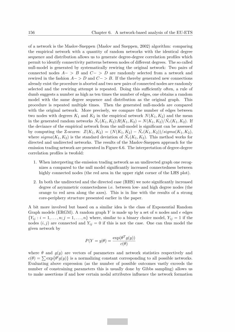
156 Chapter 6. A network-based analysis of the EU-ETS
of a network is the Maslov-Sneppen (Maslov and Sneppen, 2002) algorithm: comparingthe empirical network with a quantity of random networks with the identical degreesequence and distribution allows us to generate degree-degree correlation profiles whichpermit to identify connectivity patterns between nodes of different degrees. The so callednull-model is generated by systematically rewiring the original network: Two pairs ofconnected nodes A− > B and C− > D are randomly selected from a network andrewired in the fashion A− > D and C− > B. If the thereby generated new connectionsalready exist the procedure is aborted and two new pairs of connected nodes are randomlyselected and the rewiring attempt is repeated. Doing this sufficiently often, a rule ofdumb suggests a number as high as ten times the number of edges, one obtains a randommodel with the same degree sequence and distribution as the original graph. Thisprocedure is repeated multiple times. Then the generated null-models are comparedwith the original network. More precisely, we compare the number of edges betweentwo nodes with degrees K1 and K2 in the empirical network N(K1, K2) and the meanin the generated random networks Nr(K1, K2):R(K1, K2) = N(K1, K2)/Nr(K1, K2). Ifthe deviance of the empirical network from the null-model is significant can be assessedby computing the Z-scores: Z(K1, K2) = (N(K1, K2) − Nr(K1, K2))/sigma(K1, K2),where sigma(K1, K2) is the standard deviation of Nr(K1, K2). This method works fordirected and undirected networks. The results of the Maslov-Sneppen approach for theemission trading network are presented in Figure 6.6. The interpretation of degree-degreecorrelation profiles is twofold:
1. When interpreting the emission trading network as an undirected graph one recog-nizes a compared to the null model significantly increased connectedness betweenhighly connected nodes (the red area in the upper right corner of the LHS plot).
2. In both the undirected and the directed case (RHS) we note significantly increaseddegree of asymmetric connectedness i.e. between low- and high degree nodes (theorange to red area along the axes). This is in line with the results of a strongcore-periphery structure presented earlier in the paper.
A bit more involved but based on a similar idea is the class of Exponential RandomGraph models (ERGM). A random graph Y is made up by a set of n nodes and e edges{Yij : i = 1, . . . , n; j = 1, . . . , n} where, similar to a binary choice model, Yij = 1 if thenodes (i, j) are connected and Yij = 0 if this is not the case. One can thus model thegiven network by
P (Y = y|θ) =exp(θT g(y))
c(θ)
where θ and g(y) are vectors of parameters and network statistics respectively andc(θ) =
�exp{θtg(y)} is a normalizing constant corresponding to all possible networks.
Evaluating above expression (as the number of possible outcomes vastly exceeds thenumber of constraining parameters this is usually done by Gibbs sampling) allows usto make assertions if and how certain nodal attributes influence the network formation

6.7. Network formation 157
Figure 6.6: Degree-degree correlation profiles generated by the Maslov-Sneppen algo-rithm
process. These nodal attributes can be endogenous to the network, like the in- and out-degrees of a node, or exogenous as in the context of the trading network for example thecountry in which a specific company is registered.(Butts, 2014) We ran a basic ERGMmodel over the emission trading network. The results are presented in Table 6.6. Themost important features of the results are as following: We observe positive log-oddsfor the closing of triangles (clusters), homomophily for country and general ultimateowner (guo)respectively. We however remark negative log-odds for the formation of tiesbetween agents of the same type (i.e. OHA vs PHA). We thus see what we alreadyobserved graphically earlier in the paper: OHAs who seek to sell or buy EUAs have toaddress themselves to local networks (homophily as far as origin [country] and ownership[guo] is concerned) or to financial institutions or brokers (heterophily with regard totype).

158 Chapter 6. A network-based analysis of the EU-ETS
Dependent variable:
carbon network
edges −4.785∗∗∗
(0.172)
triangle 0.321∗∗∗
(0.026)
asymmetric −3.711∗∗∗
(0.166)
nodematch.type −0.099∗∗∗
(0.019)
nodematch.country 0.392∗∗∗
(0.031)
nodematch.guo 0.757∗∗∗
(0.285)
Akaike Inf. Crit. 527,052.300Bayesian Inf. Crit. 527,150.300
Note: ∗p<0.1; ∗∗p<0.05; ∗∗∗p<0.01
Table 6.6: A simple ERGM model applied to the ETS network
6.8 Conclusion
The of above conducted network based analysis of the European carbon market yieldedthe following central results:
1. The European carbon market network is characterized by a significant core-peripherystructure. This is on the one hand reflected in the apparent clustering behavior ofagents in the market (see Figure 6.2) and on the other in the power-law nature ofthe degree distributions (see Figure 6.3). It can however also be verified by merelylooking at the graph of the carbon market network (see Figure 6.1): We observea highly connected core, which is mainly made up by players from the financialindustry (PHAs). This core is surrounded by multiple layers of sparser connectednodes in the periphery which can be attributed to the industry (OHAs, i.e. agentswho have a legal obligation to participate in the carbon market). This layeredcore-periphery structure can also seen in the wave-like form of the various densityplots of individual-level centrality measures and profits displayed in Figure 6.4.
2. The core-periphery structure of the carbon market network is also reflected inthe network formation process. Analyzing the degree-degree correlation profilescomputed by application of the Maslov-Sneppen algorithm (see Figure 6.6) showsa strong asymmetry in the connection pattern between nodes, which is significantly

6.8. Conclusion 159
different to random null-models with the identical degree sequence and distribution:Weakly connected nodes have a tendency to connect to highly connected nodes andvice versa.
3. These results are supported when analyzing the network formation process in theEuropean carbon market network by means of an exponential random graph model(ERGM): On the one hand we observe homophily as far a origin (country in whichthe company is registered) and ownership (global ultimate owner of the company)is concerned, on the other hand heterophily for company type (industry, financeetc.).
4. It is shown that the observed network topology has an impact on the marketparticipation of agents (trading volume) as well as on the profits agents are ableto derive from trading in the market (see Figures 6.4 and 6.5).
These results in our opinion reflect one major flaw in the organization of the Europeancarbon market, which stands in stark contrast to the central idea of emission trading,namely to exploit differentials in marginal abatement costs in order to reduce the costs ofemission reduction for participating OHAs to a minimum: The European carbon marketis not organized in a central market place. The trading in the market bases, at least forthe time the data was available, to a large extent on OTC transactions. OHAs whichhave the legal obligation to participate in the carbon market are forced to resort to localnetworks or financial intermediaries. The intransparent structure of the market imposesunnecessary additional costs, for example in the form of provisions, on OHAs, whichoften don’t possess the resources to collect informations about the market themselves.The core-periphery structure of the market network should thus also be understood asa reflection of informational asymmetry in the market. This undermines the goal of theEuropean Emission Trading System to economically reduce greenhouse gas emissions
The use of network analysis is new in its application to the European Emissionmarket. Results in the literature however support our findings with regard to marketinefficiencies in the EU ETS. Hintermann (2010) for example finds that, especially inthe beginning of Phase I, EUA prices were not initially driven by abatement costs andthat new information, with regard to fundamentals, like electricity prices or weather,were only incorporated with a substantial lag, thus indicating inefficiencies in the priceformation process on the market. Palao and Pardo (2012) show the presence of priceclustering in the European Carbon Futures Markets which they interpret as a sign ofmarket inefficiency. This might be due to the weak price signal from the actual allowancemarket. Charles et al. (2013) investigate the European carbon markets, spot and futuremarkets, during Phase II with regard to cost-of-carry hypothesis. The cost-of-carrymodel is rejected in all cases implying arbitrage possibilities and thus an inefficientfunctioning of the market.
The application of methods from social network analysis to investigate the function-ing of markets in our opinion opens up a wide field of interesting questions for futureresearch. It would be for example interesting to investigate which influence the dynamic

160 Chapter 6. A network-based analysis of the EU-ETS
network structure has for the price formation or for the volatility of prices. Fitted ex-ponential random graph modelling for example allows to simulate networks which havethe same properties as the empirical network. Switching off certain factors in the sim-ulation, as for example clustering, homophily, heterophily etc., would then permit acounterfactual study to what extent certain network properties have an influence onprices (and their volatility). Such a study is planned by the authors as follow up to whatwas presented above.

Chapter 7
Conclusion
The last five chapters investigated the role of social interactions for the expectationformation (Chapters 2 to 5) and in a market context (6). This conclusive chaptersummarizes the results, outlines the methodological contributions and discusses topicsfor possible future research.
7.1 Summary, Results and Discussion
Chapter 2 In Chapter 2 it was investigated which role herding behavior plays inthe expectation formation of agents. Therefore a microlevel dataset from the Frenchhousehold survey ECAMME was transformed into a pseudo panel using self-organizingKohonen maps (Kohonen, 1982). Thereby the individuals in the data set were groupedinto cohorts which can be tracked over the whole available time frame. Basing on thecontributions by Kaiser and Spitz (2002) a technique using a MCMC hierarchical or-dered probit model was proposed to infer quantitative cohort-level estimates from thequalitative responses of survey participants with regard to their inflation expectations.A method proposed by Bernardt et al. (2006) to test herding behavior of professionalforecasters was furthermore extended in a way that it can be directly applied to thecohort-level posterior distributions of the MCMC quantification procedure. In applyingthis test it was shown, that agents overall exhibit a strong anti-herding behavior in theirexpectation formation process and thus a bias away from the consensus. Anti-herdingcorresponds to an overweighting of individual information compared to public informa-tion (the consensus or the expectations of other people). Since the study was conductedon data with regard to inflation expectations this can be attributed to the differentconsumption behavior of different sociodemographic groups which is also reflected indifferent expectations as far as the future evolution of prices is concerned. This supportsthe hypothesis of heterogenous expectations.
This result is backed by findings of other authors. Mankiw et al. (2004) for examplefinds using inter alia data from the Michigan consumer survey (this data was also usedin Chapters 3 and 4) that there is, varying with the respective economic situation,great disagreement among agents concerning expectations with regard to the future
161
162 Chapter 7. Conclusion
evolution of prices. A study by Pfajfar and Santoro (2009) finds evidence that consumersconcentrate on the CPI relevant for their sociodemographic subgroup rather than on thegeneral future inflation rate as it is surveyed by consumer surveys.
In this context it is interesting to note, that the test statistic is the closest to the mar-gin between anti-herding and herding around the third and the fourth quarter of 2008,this means at the time when the global financial crisis was triggered by the bankruptcyof the Lehman Brothers investment bank. This finding was interpreted as a result ofthe intensive media coverage of this key moment in the recent economic history, whichin the short term lead agents to attribute higher weight to public information.
Another possible interpretation of the results from Chapter 2 can be found in thework by Rülke and Tillmann (2011). The authors detect significant anti-herding behavioramong non-voting members of the Federal Open Market Committee (FOMC), which theyinterpret as some sort of strategic behavior to influence monetary policy. This mightalso apply for interviewees in consumer surveys. Being interviewed by a public entitymight be perceived by agents as one of the seldom chances to utter their opinion abouteconomic (monetary) policy and thereby to influence it to a certain degree. Given theresults in chapter 3 the interpretation with regard to heterogenous expectations howeverseems to be more likely.
Chapter 3 In Chapter 3 the panel-structure of the Michigan Consumer Survey to-gether with its questions about expectations and perceptions of the same variables wereexploited to group respondents in the dataset into “rational” and “non-rational” individ-uals in order to explore the reasons for a “rationality bias” (a deviation from rationality).For variables without backward looking question (perceptions) a Hierarchical OrderedProbit (HOPIT) method proposed by Lahiri and Zhao (2015) was used in order to esti-mate individual-level threshold values and transform the realized values of the concernedvariables (inflation and unemployment) from twelve months after the initial interviewinto individual-level perception estimates. Using a linear and non-linear Oaxaca-Blinderdecomposition (Oaxaca, 1973; Blinder, 1973; Yun, 2004; Bauer and Sinning, 2008; Rao,2009; Powers et al., 2011) the gap in expectations between “rational” and “non rational”individuals was analyzed.
It is shown that this expectational gap corresponds to an overly optimistic attitudeof “non rational” individuals and can be explained to a large and significant extent byobservable variables. These observable variables comprise sociodemographic informationas well information from questions asked during the survey. One noteworthy observationwas, that news consumption prior to the interview (a question in the Michigan ConsumerSurvey) turned out to be a significantly contributing factor in widening the rationalitygap. These findings show that the so called “rationality bias” is thus not really a questionof rationality but reflects the distinct experiences of individual agents.
It is noteworthy that this effect was weaker for variables, which to a high degreereflect the individual experience of agents, like inflation expectations or expectationswith regard to personal finance. It was argued, that this might be due to the factthat these variables are determined by factors which can impossibly be captured by a

7.1. Summary, Results and Discussion 163
standardized consumer survey. A deviation from the rationality condition applied inthis chapter might for example be due to unanticipated shocks to the financial situationof an individual. In this context one might think about maintenance work for housingor vehicles or medical bills which are connected with high costs for the individual andwhich were impossible to foresee at the date of the first interview.
These results are in line with the findings of Chapter 2 and hence also supportthe notion of heterogenous expectations. There is wide variety of both empirical andexperimental research, which backs this conclusion. The studies by Pfajfar and Santoro(2009) and Mankiw et al. (2004) are two examples which were already cited above. Thelatter is especially noteworthy as Mankiw finds evidence for heterogenous expectationsamongst others using data from the Michigan Consumer Survey which was also usedin this chapter. Branch (2004) comes to a similar conclusion. He finds that agents inthe Michigan Consumer Survey use a variety of costly predictor functions when formingtheir expectations of future price changes. Hommes (2011) uses a comparable method asBranch on experimental data, likewise showing evidence for heterogenous expectations.The same holds for the studies of Frankel and Froot (1987, 1990) and Taylor and Allen(1992), who both use data from professional forecasters.
Chapter 4 Chapter 4 however shows that the expectation formation of agents is notcompletely free from social influence. Again in applying self-organizing Kohonen maps(Kohonen, 1982), this time to the Michigan Consumer Survey, cohorts of similar indi-viduals were formed which can be traced over all the periods in which the dataset wasavailable at the time this text was written. Then transfer entropy (Schreiber, 2000), aconcept from information theory, was used, to estimate causality values (in both direc-tions) between the discrete inflation expectation time series of each cohort. The discretecohort-level time series were generated in using the cohort mean and subsequently apply-ing a discretization approach by Meyer (2008), which yields frequencies similar to thatin the whole data set. Thereby one is able to gain a notion of information flows in theexpectation formation process and thus about social influence between different cohorts.It is shown that social influence depends on sociodemographic characteristics as age,education and income. Only looking at the strongest ties in terms of net-informationtransfer one is further able to construct a network of social influence. I find that socialinfluence coincides with a high degree of connectivity and a central position within thenetwork of social influences, which as many other networks observable in reality followsa power law and thus falls into the category of scale free networks.
Chapter 5 In Chapter 5 a concept is proposed to collect economic sentiment in-formation via modern web-mining techniques in combination with approaches from ma-chine learning. The therefore created crowd-sourcing website www.insen.eu is presented,which serves the purpose of collecting human sentiment annotation for a training datasetbasing on the Reuters RCV1 corpus which can, as soon as sufficient data is available,used to train appropriate machine learning algorithms. Once this nonrecurring annota-tion and training task is terminated the algorithm can be utilized to collect sentiment

164 Chapter 7. Conclusion
information from freely available textual data on the web. It is argued that the pro-posed web based sentiment indicator is superior in multiple ways to traditional surveybased methods to collect consumer or business sentiment information: 1) The task ofdata collection is nonrecurring. As soon as the training data set is annotated, for thetime being around 600 individuals have participated in the crowdsourcing task and haveannotated 3,000 out 16,324 articles, and a machine learning algorithm was trained, themethod can be applied to an arbitrary number of new articles. Survey based sentimentindicators on the other hand rely on regularly (monthly) conducting a high number ofinterviews, which is very resource intensive. 2) Sentiment indicators can only be use-fully interpreted in the context of past data. For survey based indicators this impliesthat multiple years of data have to be collected until they can deliver any utility. Themethodology outlined here in contrast permits to analyze data, for example from web ornews archives, ex post. 3) Since the internet produces several terabytes of new relevanttextual information every day the methodology described can deliver more frequent andup-to-date sentiment information than traditional survey based sentiment indicators.
Chapter 6 In Chapter 6 the European Emission Trading System, established to eco-nomically and collectively reach the emission reduction targets as prescribed by theKyoto Protocol, is analyzed from a network perspective. In the aim to investigate theconnection between the network structure and the functioning of the market the notionof social interactions is thus brough to a market context. I find that the position ofan agent within the network has an implication for its ability to create revenues outof a trade as well as for market participation, measured as volume traded, in general.Moreover we show that the carbon market network exhibits a strong core-peripherystructure, characterized by a highly connected nodes, mainly made up by players fromthe financial industry, in the center, which is surrounded by multiple layers of weakerconnected nodes, which can mainly be attributed to the industry, in the periphery. Thistopological characteristic of the network is also reflected in an asymmetry in the match-ing process. This is evident by the presence of clustering in the graph as well as by thepower-law nature of the degree distribution. It can however also be shown by applicationof simulation based methods as the Maslov-Sneppen algorithm (Maslov and Sneppen,2002) or Exponential Random Graph Models (ERGM) (Butts, 2014), which are ableto deliver information about the network formation process: The Maslov-Sneppen ap-proach shows that the network formation process is characterized by an asymmetry inthe degree connection profiles. Weakly connected agents have a tendency to connectto highly connected agents and vice versa. Furthermore, applying an ERGM, we findheterophily as far as type (finance, industry etc.) is concerned on the on hand, ho-mophily for origin and ownership on the other hand. The above described topology ofthe network as well as the network formation process can be interpreted as some sortinformational asymmetry which is due to an inefficient functioning of the market. Inthe absence of a centralized market place, most of the transactions are over-the-counter,operators of installations which fall under the EU Emission Trading regulations have toresort to local networks or financial intermediaries if they want to buy or sell emission

7.2. Methodological Contributions 165
certificates. It is argued that this imposes unnecessary additional costs for enterprises,for example in the form of provisions to brokerage firms, which undermines the centralidea of the European Emission Trading System, namely to exploit marginal abatementcosts and to keep the costs of emission reduction to a minimum.
The application of network analysis to the European Emission Trading System isnovel. Our findings with regard to the network structure and the network formationprocess can thus unfortunately not be compared with existing studies. With regard tothe notion of market inefficiencies other authors however come to similar conclusion usingdifferent approaches. A study by Hintermann (2010) for example finds, that especiallyat the beginning of Phase I prices on the European emission market were not drivenby marginal abatement costs and that new information with regard to fundamentals,for example electricity prices or weather conditions, were only taken into account witha substantial lag. This hints to an inefficient price formation process on the market.Another study by Charles et al. (2013) tests the cost-of-carry hypothesis on severalEuropean carbon markets (spot and future markets). The hypothesis is rejected in allcases, thus indicating market inefficiency.
7.2 Methodological Contributions
In the following section an overview of the methodological contributions of this thesisshould be given.
Quantifying Inflation Expectations Consumer surveys base to a large degree onqualitative rather than quantitative questions. This has on the one hand pragmaticreasons. Most surveys, like the ECAMME (used in Chapter 2) or the Michigan Con-sumer Survey (used in Chapters 3 and 4), rely on telephone interviews. Qualitativesurvey questions thereby have the advantage that they are easily comprehensible, as theinterviewee is asked to choose one out of a limited set of, in the context of consumersurveys, normally ordered, answering options. On the other hand, as was already dis-cussed for example in Chapter 2, as far as questions with regard to the future evolutionof quantitive economic variables like the inflation rate are concerned, it turns out thatindividuals have a good sense for the trend, but often lack an accurate notion of themagnitude. The disadvantage however is, that, especially in the context of economicresearch, for some applications the qualitative survey data has to be quantified before itcan be used. This was for example the case in Chapters 2 and 3. There is a multitude ofdifferent quantification methods, which can be roughly grouped into two categories: theregression approach (see for example (Pesaran and Weale, 2006a)) and the probabilis-tic (see for example Carlson and Parkin (1975); Theil (1952); Berk (1999) ) approach.Both were already extensively discussed in Chapter 2 and 3, thus only a short overviewshould be given here. The regression approach has a row of drawbacks: First, percep-tions of price changes are assumed to be unbiased; second, it is assumed that inflationperceptions are formed along the same mechanisms as inflation expectations; third, thiswas the most important point for the research question in Chapter 2, it does not allow

166 Chapter 7. Conclusion
to control for heterogeneity within participants. The probabilistic approach, also oftendenoted as Carlson-Parkin approach, on the other hand controls for some of these issuesaddressed above. The probabilistic approach for example doesn’t make any assumptionswith regard to the mechanism the inflation expectations are formed. The unbiasednessassumption can be circumvented by appropriate calibration. The raw results of theprobabilistic approach are only identified up scale. For this reason I for example usedin Chapter 3, following Lahiri and Zhao (2015), a time varying parameter model to cal-ibrate the results. The probabilistic method however also has a number of drawbacks.In its standard implementation it as well doesn’t allow to control for the heterogeneityof agents, it can’t be estimated as soon as one answering option is completely missingin one period and the thresholds of the indifference limens are assumed to be symmetricand constant. Kaiser and Spitz (2002) show that the probabilistic method can also beestimated in an ordered probit framework which solves these issues. In Chapter 2 I showthat this approach can be extended to a Hierarchical Bayes Markov Chain Monte CarloOrdered Probit model. This has the same advantages as the method by Kaiser andSpitz (2002), however, by the inclusion of random intercepts allows to quantify qualita-tive inflation expectations on an individual- or, in the context of this study, cohort-level.This is the main difference to the maximum likelihood method along Lahiri and Zhao(2015) used in 3. Furthermore, it can handle relatively small amounts of cohort-leveldata and still gives good estimates as it borrows information from the whole popula-tion to gain individual-level or here cohort-level estimates. One can moreover run verycomplex estimations. The inclusion of explanatory variables is only limited by hardwarerestrictions.
Testing herding behavior on huge data sets The central method in Chapter2 is the herding test proposed by Bernardt et al. (2006). It relies on the estimationof conditional probabilities with regard to the overshooting/undershooting of agents’inflation expectations compared to the consensus (see Section 2.3). In Section 2.8 itis shown how the test statistic by Bernardt et al. (2006) can be reformulated to arank sum test in the style of the Wilcoxon test. This test shares the same statisticalproperties as the original test statistic by Bernardt et al. (2006), but can be computed,even for extremely large data sets, within seconds. In the context of Chapter 2 it wasdirectly applied to the posterior distributions of cohort-level inflation estimates resultingfrom the Hierarchical Ordered Probit MCMC estimation. Moreover, in contrast to theoriginal herding test by Bernardt et al. (2006) there is no concrete consensus value. Theconsensus is normally the mean or median of all extant forecasts for the same targetvalue. In my modification of the test statistic the information of the entire posteriordistributions of all other cohorts, when estimated for a single cohort, is exploited.
Inferring networks of influence from survey data Chapter 4 demonstrates a wayto apply information theory, namely the concept of transfer entropy by Schreiber (2000),to consumers surveys in order to infer networks of influence. Barnett et al. (2009) showthat transfer entropy is exactly equivalent to Granger causality for variables following

7.3. Topics for future Research 167
a Gaussian distribution. In its application to survey data transfer entropy however hasthe big advantage, that it can directly be applied to discrete variables, which spares theuse of quantification methods as it was necessary in the chapters 2 and 3.
Using text mining and machine learning to collect sentiment data Chapter5 shows how modern text mining and machine learning methods can be employed tocollect sentiment data from textual information on the internet. The proposed webbased sentiment indicator is more cost efficient, as the task of data gathering directlyfrom individuals is nonrecurring, and can deliver more frequent and up-to-date sentimentinformation than traditional survey based sentiment indicators.
A network based analysis of market In Chapter 6 finally my coauthors StefanoBattiston, Antoine Mandel and me show how network science can be applied to analyzethe structure and functioning of markets. This in our opinion has advantages to anoutcome based analysis, multiple examples of such studies are cited in the conclusion ofChapter 6, as it allows to evaluate the micro structure as well as the matching processesat work on the market.
7.3 Topics for future Research
The work presented above opens up a range of interesting questions for future research.Some ideas should be discussed in what follows.
In chapters 2 and 3 I find that the expectation formation of agents is characterized bysignificant heterogeneity, a result supported by findings in other studies. In the contextof Chapter 2 this heterogeneity of expectations with regard to inflation is reflected in asignificant anti-herding behavior of agents, which was interpreted as due to the differentconsumption behavior of individuals. Especially in the context of the results aroundthe third and the fourth quarter of 2008, when the global financial crisis started (seediscussion above), it would interesting to repeat this study for a variable which is moregeneral, like the general business condition for example, and thus doesn’t reflect so muchon the individual financial situation of agents.
Furthermore it would be interesting to extend the methods of social network analysisemployed in Chapter 6 for the analysis of the European carbon market, to a dynamicview of the market network. This would allow to investigate which influence the dynamicevolution of the network structure has for the price formation or for the volatility ofprices. Together with the simulation from a fitted exponential random graph model thiswould permit to conduct a counterfactual analysis with regard to what factors in thenetwork structure or in the network formation process have an influence on the marketprices and their volatility respectively. Such a study is planned by the authors as followup to what was presented above.
The transfer entropy measure used in Chapter 4 to infer a network of influence withregard to the formation of inflation expectations could also be applied in a non-economiccontext. The author for example already tested the same methodology to infer networks

168 Chapter 7. Conclusion
of influence in the European Parliament using data from roll-call votes. This could forexample serve to investigate the cooperation of members of the parliament aside partyaffiliations. A study of this kind is planned for the near future.

List of Figures
2.1 Schematic plot of the idea behind the herding test by Bernardt et al. (2006) 192.2 Threshold model with a standard normal distribution . . . . . . . . . . . 282.3 Plot of the self organizing Kohonen map . . . . . . . . . . . . . . . . . . . 302.4 Raw estimates of perceptions and expectations; differentiated perceptions
vs. expectations - Jan 2004 to Dec 2012 . . . . . . . . . . . . . . . . . . . 372.5 Correlation - Perceptions vs. actual Inflation - Jan 2004 to Dec 2012 . . . 382.6 Correlation - Expectations vs. differentiated Perceptions - Jan 2004 to
Dec 2012 . . . . . . . . . . . . . . . . . . . . . . . . . . . . . . . . . . . . 392.7 Cohort-level inflation perceptions and actual inflation - Jan 2004 to Dec
2012 . . . . . . . . . . . . . . . . . . . . . . . . . . . . . . . . . . . . . . . 402.8 Cohort-level inflation expectations and actual inflation - Jan 2004 to Dec
2012 . . . . . . . . . . . . . . . . . . . . . . . . . . . . . . . . . . . . . . . 412.9 Quarterly Herding Test Statistic - Jan 2004 to Dec 2012 (5% confidence
interval) . . . . . . . . . . . . . . . . . . . . . . . . . . . . . . . . . . . . . 452.10 Perceived inflation vs. actual inflation for each cohort . . . . . . . . . . . 552.11 Expected inflation vs. actual inflation for each cohort . . . . . . . . . . . 56
3.1 Quantification of qualitative expectations of the inflation rate with theHOPIT method (the shaded areas in the plot correspond to the recessionperiods along the definition of the Federal Reserve Bank) . . . . . . . . . 71
3.2 Quantification of qualitative expectations of the unemployment rate withthe HOPIT method (the shaded areas in the plot correspond to the re-cession periods along the definition of the Federal Reserve Bank) . . . . . 72
3.3 Optimism, Pessimism and Rationality over time (the shaded areas in theplot correspond to the recession periods along the definition of the FederalReserve Bank) . . . . . . . . . . . . . . . . . . . . . . . . . . . . . . . . . 73
4.1 Information transfer between social groups with different educational back-ground (x-Axis: sender education; y-Axis: receiver education; green: lowinformation transfer; red: high information transfer). . . . . . . . . . . . . 104
4.2 Information transfer between social groups with different income (x-Axis:sender income; y-Axis: receiver income; green: low information transfer;red: high information transfer) . . . . . . . . . . . . . . . . . . . . . . . . 105
169

170 List of Figures
4.3 Information transfer between social groups with different age (x-Axis:sender age; y-Axis: receiver age; green: low information transfer; red:high information transfer) . . . . . . . . . . . . . . . . . . . . . . . . . . . 106
4.4 The network of social influence as estimated by the University of Michiganconsumer Survey . . . . . . . . . . . . . . . . . . . . . . . . . . . . . . . . 107
4.5 Cumulative degree distribution with power law fitted (log-scale) . . . . . . 1084.6 The Social Network in the form of ordered arcplots . . . . . . . . . . . . . 1094.7 Degree, betweenness, eigenvector, closeness centrality as a function of age,
education and yearly income in USD . . . . . . . . . . . . . . . . . . . . . 1114.8 Information Transfer under consideration of different time lags . . . . . . 112
5.1 Flowchart of the Procedure . . . . . . . . . . . . . . . . . . . . . . . . . . 1215.2 Principle of SVM . . . . . . . . . . . . . . . . . . . . . . . . . . . . . . . . 1255.3 Startpage of the insen.eu crowdsourcing website . . . . . . . . . . . . . . . 1305.4 Selecting the respective study on www.insen.eu . . . . . . . . . . . . . . . 1315.5 Sociodemographic data collected by the www.insen.eu crowdsourcing web-
site . . . . . . . . . . . . . . . . . . . . . . . . . . . . . . . . . . . . . . . . 1325.6 Annotating sentiments to RCV1 articles on www.insen.eu . . . . . . . . . 134
6.1 The CO2 trading network [CDM (green),finance (red),foundation (yel-low), government (orange), industry (blue)] . . . . . . . . . . . . . . . . . 151
6.2 In-/Out-Degree vs. Cliquishness (in-degree: blue; out-degree: red) . . . . 1526.3 In-/Out-/Total-Degree distribution with fitted power law . . . . . . . . . 1536.4 Densities plots for various trade network statistics and company types in
the ETS . . . . . . . . . . . . . . . . . . . . . . . . . . . . . . . . . . . . . 1546.5 Elevation plots of out- (u) and in- (v) coreness values with respect to
the generated profits and market participation (total volume traded) ofindividual agents . . . . . . . . . . . . . . . . . . . . . . . . . . . . . . . . 155
6.6 Degree-degree correlation profiles generated by the Maslov-Sneppen algo-rithm . . . . . . . . . . . . . . . . . . . . . . . . . . . . . . . . . . . . . . 157

List of Tables
2.1 Descriptive Statistics - ECAMME data set (Jan 2004 - Dec 2012) . . . . . 182.2 Descriptive Statistics - Income - ECAMME data set (Jan 2004 - Dec 2012) 182.3 Contingency table - expectations j vs. perceptions i . . . . . . . . . . . . 222.4 Perception estimation - Fixed effects [Signif. codes: 0 ∗∗∗, 0.001 ∗∗, 0.01
∗, 0.05 . 0.1] . . . . . . . . . . . . . . . . . . . . . . . . . . . . . . . . . . . 342.5 Expectation estimation - Fixed effects [Signif. codes: 0 ∗∗∗, 0.001 ∗∗, 0.01
∗, 0.05 . 0.1] . . . . . . . . . . . . . . . . . . . . . . . . . . . . . . . . . . . 352.6 Heidelberger/Welch Stationarity Test and Halfwidth Test . . . . . . . . . 362.7 Results - test statistics . . . . . . . . . . . . . . . . . . . . . . . . . . . . . 44
3.1 University of Michigan Consumer Survey: Descriptive Statistics . . . . . . 583.2 Linear decomposition of the expectation bias - consumer prices (reference
group) . . . . . . . . . . . . . . . . . . . . . . . . . . . . . . . . . . . . . . 793.3 Linear decomposition of the expectation bias - consumer prices (Neumark) 793.4 Non-Linear decomposition of the expectation bias - consumer prices (ref-
erence group) . . . . . . . . . . . . . . . . . . . . . . . . . . . . . . . . . . 803.5 Non-Linear decomposition of the expectation bias - consumer prices (Neu-
mark) . . . . . . . . . . . . . . . . . . . . . . . . . . . . . . . . . . . . . . 803.6 Non-Linear decomposition of the expectation bias - personal finances (ref-
erence group) . . . . . . . . . . . . . . . . . . . . . . . . . . . . . . . . . . 813.7 Non-Linear decomposition of the expectation bias - personal finances
(Neumark) . . . . . . . . . . . . . . . . . . . . . . . . . . . . . . . . . . . 813.8 Non-Linear decomposition of the expectation bias - business climate (ref-
erence group) . . . . . . . . . . . . . . . . . . . . . . . . . . . . . . . . . . 823.9 Non-Linear decomposition of the expectation bias - business climate (Neu-
mark) . . . . . . . . . . . . . . . . . . . . . . . . . . . . . . . . . . . . . . 823.10 Non-Linear decomposition of the expectation bias - unemployment rate
(reference group) . . . . . . . . . . . . . . . . . . . . . . . . . . . . . . . . 833.11 Non-Linear decomposition of the expectation bias - unemployment (Neu-
mark) . . . . . . . . . . . . . . . . . . . . . . . . . . . . . . . . . . . . . . 833.12 HOPIT parameter estimates: consumer prices . . . . . . . . . . . . . . . . 933.13 HOPIT parameter estimates: consumer prices . . . . . . . . . . . . . . . . 94
171

172 List of Tables
4.1 University of Michigan Consumer Survey: Descriptive Statistics . . . . . . 964.2 Transfer Entropies: split up by education and age . . . . . . . . . . . . . . 1034.3 Transfer Entropies: by income, education and age . . . . . . . . . . . . . . 103
5.1 Example of a binary term matrix . . . . . . . . . . . . . . . . . . . . . . . 123
6.1 Quantified emission limitation or reduction commitment (percentage ofbase year or period) (United Nations, 1998, 2012) . . . . . . . . . . . . . . 141
6.2 Joint Implementation projects and issued ERUs in selected countries (Source:Centre (2014)) . . . . . . . . . . . . . . . . . . . . . . . . . . . . . . . . . 143
6.3 Clean Development Mechanism project and issued CERs by world region(Source: Centre (2014)) . . . . . . . . . . . . . . . . . . . . . . . . . . . . 143
6.4 Emission Reduction Targets of the EU-15 along the Burden Sharing Agree-ment from 1998 with regard to the respective base years (given as per-centage of the base year emissions) (European Council, 1998) . . . . . . . 145
6.5 Sequence of the European Emission Trading Scheme over a trading period(Trotignon and Delbosc, 2008, p. 5) . . . . . . . . . . . . . . . . . . . . . 150
6.6 A simple ERGM model applied to the ETS network . . . . . . . . . . . . 158

Bibliography
Anderson, Oskar, J., 1952. The business test of the ifo-institute for economic research,munich, and its theoretical model. Revue de l’Institut International de Statistique /Review of the International Statistical Institute 20, pp. 1–17.
Ang, A., Bekaert, G., Wei, M., 2007. Do macro variables, asset markets, or surveysforecast inflation better? Journal of Monetary Economics 54, pp. 1163–1212.
Asch, S.E., 1951. Effects of group pressure upon the modification and distortion ofjudgments, in: Guetzkow, H. (Ed.), Groups, Leadership and Men; Research in HumanRelations. Carnegie Press Groups, Oxford, England, pp. pp. 222–236.
Baghestani, H., 2009. Survey evidence on the Muthian rationality of the inflation fore-casts of US consumers. Oxford Bulletin of Economics and Statistics 54, pp. 173–186.
Barnett, L., Barrett, A.B., Seth, A.K., 2009. Granger causality and transfer entropy areequivalent for gaussian variables. Physical Review Letters 103.
Batchelor, R., 1986. The psychophysics of inflation. Journal of Economic Psychology 7,pp. 269–290.
Batchelor, R., 2001. How useful are the forecasts of intergovernmental agencies? TheIMF and OECD versus the consensus. Applied Economics 33, pp. 225–235.
Bates, J., Granger, C., 1969. The combination of forecasts. Operational ResearchQuarterly 20, pp. 451–468.
Bauer, T.K., Sinning, M., 2008. An extension of the Blinder–Oaxaca decomposition tononlinear models. AStA Advances in Statistical Analysis 92, pp. 197–206.
Beaudry, P., Portier, F., 2004. An exploration into Pigou’s theory of cycles. Journal ofMonetary Economics 51, pp. 1183–1216.
Beaudry, P., Portier, F., 2006. News, stock prices and economic fluctuations. AmericanEconomic Review 96, pp. 1293–1307.
Berk, J.M., 1999. Measuring inflation expectations: a survey data approach. AppliedEconomics 31, pp. 1467–1480.
173

174 Bibliography
Bernardt, D., Campello, M., Kutsoati, E., 2006. Who herds? Journal of FinancialEconomics 80, pp. 657–675.
Blinder, A.S., 1973. Wage discrimination: reduced form and structural estimates. Jour-nal of Human Resources , pp. 436–455.
Blood, D., Phillips, P., 1995. Recession headline news, consumer sentiment, the state ofthe economy and presidential popularity: a time series analysis 1989–1993. Interna-tional Journal of Public Opinion research 7, 2.
Bonacich, P., 1987. Power and centrality: A family of measures. American Journal ofSociology , pp. 1170–1182.
Bonham, C., Cohen, R., 2001. To aggregate, pool, or neither. Journal of Business andEconomic Statistics 19, pp. 278–291.
Borgatti, S.P., 2005. Centrality and network flow. Social networks 27, pp. 55–71.
Boyd, J.P., Fitzgerald, W.J., Mahutga, M.C., Smith, D.A., 2010. Computing contin-uous core/periphery structures for social relations data with MINRES/SVD. SocialNetworks 32, pp. 125–137.
Branch, W.A., 2004. The Theory of Rationally Heterogeneous Expectations: Evidencefrom Survey Data on Inflation Expectations. The Economic Journal 114, pp. 592–621.
Breiman, L., 2001. Random forests. Machine Learning 45, pp. 5–32.
Burges, C.J., 1998. A tutorial on support vector machines for pattern recognition. DataMining and Knowledge Discovery 2, pp. 121–167.
Burnkrant, R.E., Cousineau, A., 1975. Informational and normative social influence inbuyer behavior. Journal of Consumer Research , pp. 206–215.
Butts, C.T., 2014. Introduction to exponential-family random graph (erg or p*) modelingwith ergm. European University Institute, Florence. URL: http://cran.r-project.
org/web/packages/ergm/vignettes/ergm.pdf.
Capistrán, C., Timmermann, A., 2009. Disagreement and biases in inflation expecta-tions. Journal of Money, Credit and Banking 41, pp. 365–396.
Cardie, C., Farina, C., Bruce, T., 2006. Using natural language processing to improveerulemaking: project highlight, in: Proceedings of the 2006 international conferenceon Digital government research, Digital Government Society of North America. pp.177–178.
Carlson, J., Parkin, M., 1975. Inflation expectations. Economica 42, pp. 123–138.

Bibliography 175
Carnazza, P., Parigi, G., 2002. Towards the elaboration of business climate indicatorsfor the italian economy, in: Poser, G., Bloesch, D. (Eds.), Economic surveys and dataanalysis: CIRET Conference proceedings, Paris 2000, Organization for Economic Co-operation and Development. p. pp. 33.
Carroll, C., 2003. Macroeconomic expectations of households and professional forecast-ers. Quarterly Journal of Economics 118, pp. 269–298.
Centre, U.R., 2014. JI & CDM projects. URL: http://www.cdmpipeline.org/. [online;2015-09-29].
Charles, A., Darné, O., Fouilloux, J., 2013. Market efficiency in the european carbonmarkets. Energy Policy 60, pp. 785–792.
Choi, H., Varian, H., 2012. Predicting the present with google trends. Economic Record88, pp. 2–9.
Clauset, A., Shalizi, C.R., Newman, M.E., 2009. Power-law distributions in empiricaldata. SIAM Review 51, pp. 661–703.
Cleveland, W.S., Grosse, E., Shyu, W.M., 1992. Local regression models. StatisticalModels in S , pp. 309–376.
Coibion, O., Gorodnichenko, Y., 2012. What can survey forecasts tell us about informa-tion rigidities? Journal of Political Economy 120, pp. 116–159.
Collard, D., 1983. Pigou on expectations and the cycle. The Economic Journal 93, pp.411–414.
Cotton, J., 1988. On the decomposition of wage differentials. The Review of Economicsand Statistics , pp. 236–243.
Cottrell, M., Gaubert, P., 2007. Efficient estimators: the use of neural networks toconstruct pseudo panels. arXiv preprint math/0701154 .
Cover, T.M., Thomas, J.A., 1991. Elements of information theory. John Wiley & Sons.
Cunningham, H., Maynard, D., Bontcheva, K., Tablan, V., 2002. Gate: an architec-ture for development of robust hlt applications, in: Proceedings of the 40th AnnualMeeting on Association for Computational Linguistics, Association for ComputationalLinguistics. pp. pp. 168–175.
Curto Millet, F., 2009. Finding the optimal method of quantifying inflation expectationson the basis of qualitative survey data, in: Sinclair, P. (Ed.), Inflation Expectations,Routledge, London.
Deaton, A., 1985. Panel data from time series of cross-sections. Journal of Econometrics30, pp. 109–126.

176 Bibliography
Debreu, G., 1974. Excess demand functions. Journal of mathematical economics 1, pp.15–21.
Doms, M., Morin, N., 2004. Consumer sentiment, the economy, and the news media.FEDS working paper 2004.
Dornbusch, R., 1976. Expectations and exchange rate dynamics. The Journal of PoliticalEconomy 84, pp. 1161–1176.
Duan, K., Keerthi, S., 2005. Which is the best multiclass svm method? an empiricalstudy, in: Oza, N., Polikar, R., Kittler, J., Roli, F. (Eds.), Multiple classifier systems:proceedings of the 6th international workshop, MCS 2005, Seaside, CA, USA, June13-15, 2005, Springer Inc., New York. pp. pp. 278–285.
EC, 2006. European economy - special report. European Commission Directorate-General for Economic and Financial Affairs .
EC, 2007. The joint harmonized eu programme of business and consumer surveys (userguide). European Commission Directorate-General for Economic and Financial Affairs.
Einav, L., Levin, J.D., 2013. The data revolution and economic analysis. Working Paperw19035. National Bureau of Economic Research.
Ellerman, A.D., 2010. Pricing carbon: the European Union emissions trading scheme.Cambridge University Press.
Ellerman, A.D., Buchner, B., 2007. The european union emissions trading scheme:origins, allocation, and early results. Review of Environmental Economics and Policy1, pp. 66–87.
Ellerman, A.D., Decaux, A., 1998. Analysis of post-kyoto co2 emissions trading usingmarginal abatement curves. (working paper) .
Ellerman, A.D., Joskow, P.L., 2008. The European Union’s emissions trading system inperspective. Pew Center on Global Climate Change Arlington, VA.
Eluru, N., Bhat, C.R., Hensher, D.A., 2008. A mixed generalized ordered response modelfor examining pedestrian and bicyclist injury severity level in traffic crashes. AccidentAnalysis & Prevention 40, pp. 1033–1054.
European Commission, 1998. Communication of 3 june 1998 from the commission tothe council and the European Parliament - climate change - towards an EU post-Kyoto strategy. URL: http://eur-lex.europa.eu/legal-content/EN/TXT/PDF/
?uri=CELEX:51998DC0353&from=EN.

Bibliography 177
European Commission, 1999. Communication of 19 may 1999 from the commission tothe council and the European Parliament - preparing for implementation of the KyotoProtocol. URL: http://ec.europa.eu/clima/policies/ets/docs/com_1999_230_
en.pdf.
European Commission, 2000. Green paper on greenhouse gas emissions trading withinthe european union. URL: http://eur-lex.europa.eu/legal-content/EN/TXT/
PDF/?uri=CELEX:52000DC0087&qid=1400357223266&from=EN.
European Commission, 2002. 2002/358/EC: Council decision of 25 april 2002 concerningthe approval, on behalf of the european community, of the kyoto protocol to theunited nations framework convention on climate change and the joint fulfilment ofcommitments thereunder. URL: http://eur-lex.europa.eu/legal-content/EN/
TXT/PDF/?uri=CELEX:32002D0358&from=EN.
European Commission, 2008a. Directive 2008/101/EC of the european parliament andof the council of 19 november 2008 amending directive 2003/87/ec so as to include avi-ation activities in the scheme for greenhouse gas emission allowance trading within thecommunity. URL: http://eur-lex.europa.eu/legal-content/EN/TXT/PDF/?uri=
CELEX:32008L0101&from=EN.
European Commission, 2008b. The EU Emissions Trading System (EU ETS). URL:http://ec.europa.eu/clima/publications/docs/factsheet_ets_en.pdf.
European Commission, 2009. Directive 2009/29/EC of the European parliament andof the council of 23 april 2009 amending directive 2003/87/EC so as to improveand extend the greenhouse gas emission allowance trading scheme of the com-munity. URL: http://eur-lex.europa.eu/LexUriServ/LexUriServ.do?uri=OJ:L:
2009:140:0063:0087:en:PDF.
European Council, 1993a. 93/389/EEC: Council Decision of 24 June 1993for a monitoring mechanism of Community CO2 and other greenhouse gasemissions. URL: http://eur-lex.europa.eu/legal-content/EN/TXT/PDF/?uri=
CELEX:31993D0389&from=EN.
European Council, 1993b. 94/69/EC: Council Decision of 15 December 1993 con-cerning the conclusion of the United Nations Framework Convention on ClimateChange . URL: http://eur-lex.europa.eu/legal-content/EN/TXT/?uri=CELEX:
31994D0069.
European Council, 1996. Council directive 96/61/ec of 24 september 1996concerning integrated pollution prevention and control. URL: http:
//eur-lex.europa.eu/legal-content/EN/TXT/PDF/?uri=CELEX:31996L0061&
qid=1400338366270&from=EN.
European Council, 1998. 2106th Council meeting ENVIRONMENT Luxembourg, 16-17June 1998. URL: http://europa.eu/rapid/press-release_PRES-98-205_en.pdf.

178 Bibliography
European Parliament, 2003. Directive 2003/87/EC of the European Parliament andthe Council of 13 October 2003 establishing a scheme for greenhouse gas emis-sion allowance trading within the Community and amending Council Directive96/61/EC. URL: http://eur-lex.europa.eu/legal-content/EN/TXT/PDF/?uri=
CELEX:02003L0087-20090625&from=EN.
European Parliament, 2004. Directive 2004/101/EC of the European Parliament and ofthe Council of 27 October 2004 amending Directive 2003/87/EC establishing a schemefor greenhouse gas emission allowance trading within the Community, in respect ofthe Kyoto ProtocolâĂŹs project mechanisms. URL: http://eur-lex.europa.eu/
legal-content/EN/TXT/PDF/?uri=CELEX:32004L0101&from=en.
European Union, 1986. Single European Act. URL: http://eur-lex.europa.eu/
resource.html?uri=cellar:7734bd6d-1870-4310-9b8c-db6214b1918d.0006.01/
DOC_1&format=PDF.
Evans, G.W., Honkapohja, S., 2001. Learning and expectations in macroeconomics.Princeton University Press.
Fan, D., Cook, R., 2003. A differential equation model for predicting public opinionsand behaviors from persuasive information: application to the Index of ConsumerSentiment. The Journal of Mathematical Sociology 27, pp. 29–51.
Feinerer, I., Hornik, K., Meyer, D., 2008. Text mining infrastructure in r. Journal ofStatistical Software 25, pp. 1–54.
Fischer, B., 1995. Decomposition of time series: comparing different methods in theoryand practice. Eurostat.
Fisher, I., 1911. The Purchasing Power of Money. The Macmillan Co., New York.
Forsells, M., Kenny, G., 2002. The rationality of consumers’ inflation expectations:survey-based evidence for the euro area. Working Paper 163. European Central Bank.
Fournier, D.A., Skaug, H.J., Ancheta, J., Ianelli, J., Magnusson, A., Maunder, M.N.,Nielsen, A., Sibert, J., 2012. AD Model Builder: using automatic differentiation forstatistical inference of highly parameterized complex nonlinear models. OptimizationMethods and Software 27, pp. 233–249.
Franke, R., et al., 2008. A microfounded herding model and its estimation on germansurvey expectations. Intervention: European Journal of Economics and EconomicPolicies 5, pp. 305–332.
Frankel, J.A., Froot, K.A., 1987. Short-term and long-term expectations of the yen/dol-lar exchange rate: evidence from survey data. Journal of the Japanese and Interna-tional Economies 1, pp. 249–274.

Bibliography 179
Frankel, J.A., Froot, K.A., 1990. Chartists, fundamentalists, and trading in the foreignexchange market. The American Economic Review 80, pp. 181–185.
Freeman, L.C., 1979. Centrality in social networks conceptual clarification. Social Net-works 1, pp. 215–239.
Friedman, M., 1968. The role of monetary policy. The American Economic Review 58,pp. 1–17.
Gardes, F., Gaubert, P., Rousset, P., 1996. Cellulage de données d’enquêtes de consom-mation par une méthode neuronale. Rapport de recherche pour le CREDOC .
Gardes, F., Ghabri, S., Madre, J., Pichery, M., 2000. Rationality of price and unem-ployment expectations: tests on French qualitative microdata, in: Gardes, F., Prat,G. (Eds.), Price expectations in goods and financial markets. Edward Elgar, pp. pp.131–155.
Gardes, F., Madre, J., 1991. Les anticipations des ménages dans les enquêtes de con-joncture de l’insee. Economie et Prévision 99, pp. 1–29.
Ghose, A., Ipeirotis, P., Sundararajan, A., 2007. Opinion mining using econometrics: Acase study on reputation systems, in: Annual Meeting-Association for ComputationalLinguistics, p. pp. 416.
Gill, J., King, G., 2004. What to do when your hessian is not invertible. SociologicalMethods & Research 32, pp. 1–34.
Gourieroux, C., Pradel, J., 1986. Direct test of the rational expectation hypothesis.European Economic Review 30, 265–284.
Greene, W.H., Hensher, D.A., 2010. Ordered choices and heterogeneity in attributeprocessing. Journal of Transport Economics and Policy (JTEP) 44, pp. 331–364.
Grisse, C., 2009. Are expectations about economic activity selffulfilling? An empiricaltest. Technical Report. Mimeo. Federal Reserve Bank of New York.
Gullì, F., 2009. Markets for carbon and power pricing in Europe: theoretical issues andempirical analyses. Edward Elgar Publishing.
Hadfield, J.D., 2010. MCMC Methods for Multi-Response Generalized Linear MixedModels: The MCMCglmm R Package. Journal of Statistical Software 33, pp. 1–22.URL: http://www.jstatsoft.org/v33/i02/.
Heidelberger, P., Welch, P.D., 1981. A spectral method for confidence interval generationand run length control in simulations. Communications of the ACM 24, pp. 233–245.
Hintermann, B., 2010. Allowance price drivers in the first phase of the EU ETS. Journalof Environmental Economics and Management 59, pp. 43–56.

180 Bibliography
Hirschfeld, G., Bien, H., de Vries, M., Lüttmann, H., Schwall, J., 2010. Open-sourcesoftware to conduct online rating studies. Behavior Research Methods 42, pp. 542–546.
Hommes, C., 2011. The heterogeneous expectations hypothesis: Some evidence from thelab. Journal of Economic dynamics and control 35, pp. 1–24.
Howrey, E., 2001. The predictive power of the index of consumer sentiment. Brookingspapers on economic activity 2001, pp. 175–216.
Hyman, H.H., 1942. The psychology of status. Archives of Psychology 269.
Jackson, M.O., 2008. Social and economic networks. Princeton University Press.
Jahoda, M., 1959. Conformity and independence. Human Relations 12, pp. 99–120.
Jaimovich, N., Rebelo, S., 2009. Can News about the Future Drive the Business Cycle?American Economic Review 99, pp. 1097–1118.
Jann, B., 2008. A Stata implementation of the Blinder-Oaxaca decomposition. StataJournal 8, pp. 453–479.
Jaraite, J., Jong, T., Kazukauskas, A., Zaklan, A., Zeitlberger, A., 2013. OwnershipLinks and Enhanced EUTL Dataset. European University Institute, Florence. URL:http://fsr.eui.eu/CPRU/EUTLTransactionData.aspx.
Jones, R.C., 2014. Making Better (Investment) Decisions. The Journal of PortfolioManagement 40, pp. 128–143.
Kaiser, U., Spitz, A., 2002. Quantification of Qualitative Data Using Ordered ProbitModels, in: Economic surveys and data analysis: CIRET Conference proceedings,Paris 2000, Organization for Economic. p. pp. 325.
Karpf, A., 2013. Herd behavior in consumer inflation expectations - Evidence from theFrench household survey. Documents de travail du Centre d’Economie de la Sorbonne13054R. Université Panthéon-Sorbonne (Paris 1), Centre d’Economie de la Sorbonne.URL: ftp://mse.univ-paris1.fr/pub/mse/CES2013/13054R.pdf.
Karpf, A., 2014. Expectation Formation and Social Influence. Documents de travaildu Centre d’Economie de la Sorbonne 14005. Université Panthéon-Sorbonne (Paris1), Centre d’Economie de la Sorbonne. URL: ftp://mse.univ-paris1.fr/pub/mse/
CES2014/14005.pdf.
Katona, G., 1974. Psychology and consumer economics. The Journal of ConsumerResearch 1, pp. 1–8.
Keynes, J., 1936. The general theory of employment, money and interest. Macmillan,London.
Knight, F., 1921. Risk, Uncertainty and Profit. Houghton Mifflin & Co, New York.

Bibliography 181
Kohonen, T., 1982. Self-organized formation of topologically correct feature maps. Bio-logical Cybernetics 43, pp. 59–69.
Kohonen, T., 2001. Self-organizing maps. volume 30. Springer, Berlin.
Koppel, M., Shtrimberg, I., 2006. Good news or bad news? Let the market decide, in:Computing attitude and affect in text: Theory and applications. Springer, pp. pp.297–301.
Kullback, S., 1959. Information theory and statistics. John Wiley & Sons.
Kwon, N., Shulman, S., Hovy, E., 2006. Multidimensional text analysis for eRulemaking,in: Proceedings of the 2006 international conference on Digital government research,ACM. pp. pp. 157–166.
Lahiri, K., Zhao, Y., 2015. Quantifying survey expectations: A critical review andgeneralization of the Carlson–Parkin method. International Journal of Forecasting 31,pp. 51–62.
Lee, L., 2004. " I’m sorry Dave, I’m afraid I can’t do that": Linguistics, Statistics,and Natural Language Processing circa 2001, in: Computer Science: Reflections onthe Field, Reflections from the Field, Committee on the Fundamentals of ComputerScience: Challenges and Opportunities, Computer Science and TelecommunicationsBoard, National Research Council. The National Academics Press. pp. pp. 111–118.
Lewis, D., Yang, Y., Rose, T., Li, F., 2004. RCV1: A new benchmark collection for textcategorization research. The Journal of Machine Learning Research 5, pp. 361–397.
Li, D., Schürhoff, N., 2014. Dealer networks .
Lucas, R., 1976. Econometric policy evaluation: A critique, in: Carnegie-RochesterConference Series on Public Policy, pp. pp. 19–46.
Ludvigson, S., 2004. Consumer confidence and consumer spending. The Journal ofEconomic Perspectives 18, pp. 29–50.
Maag, T., 2009. On the accuracy of the probability method for quantifying beliefs aboutinflation. ETH, Eidgenössische Technische Hochschule Zürich, KOF Swiss EconomicInstitute.
Maddala, G., 1991. Survey data on expectations: what have we learnt? Issues inContemporary Economics 2, pp. 319–344.
Mankiw, N., Reis, R., 2002. Sticky information versus sticky prices: a proposal toreplace the New Keynesian Phillips curve. The Quarterly Journal of Economics 117,pp. 1295–1328.
Mankiw, N.G., Reis, R., Wolfers, J., 2004. Disagreement about inflation expectations,in: NBER Macroeconomics Annual 2003, Volume 18. The MIT Press, pp. pp. 209–270.

182 Bibliography
Manski, C.F., 2000. Economic analysis of social interactions. The Journal of EconomicPerspectives 14, pp. 115–136.
Mantel, R.R., 1974. On the characterization of aggregate excess demand. Journal ofEconomic Theory 7, pp. 348–353.
Maslov, S., Sneppen, K., 2002. Specificity and stability in topology of protein networks.Science 296, pp. 910–913.
Masuyama, T., Nakagawa, H., 2004. Two step pos selection for svm based text catego-rization. IEICE TRANSACTIONS on Information and Systems 87, pp. 373–379.
Matsusaka, J., Sbordone, A., 1995. Consumer confidence and economic fluctuations.Economic Inquiry 33, pp. 296–318.
Mehkari, M.S., 2010. Markups, Dynamic Demand Curves, News Shocks, and BusinessCycles. Department of Economics, Ohio State University (working paper) .
Mehra, Y.P., 2002. Survey measures of expected inflation: revisiting the issues of pre-dictive content and rationality. FRB Richmond Economic Quarterly 88, pp. 17–36.
Merton, R.K., 1968. Social theory and social structure. Simon and Schuster.
Meyer, P.E., 2008. Information-theoretic variable selection and network inference frommicroarray data. Ph.D. thesis. Université Libre de Bruxelles. Brussels, Belgium.
Mierswa, I., Wurst, M., Klinkenberg, R., Scholz, M., Euler, T., 2006. YALE: Rapidprototyping for complex data mining tasks, in: Proceedings of the 12th ACM SIGKDDinternational conference on Knowledge discovery and data mining, ACM. pp. pp. 935—940.
Mishne, G., Glance, N., 2006. Predicting movie sales from blogger sentiment, in: AAAI2006 Spring Symposium on Computational Approaches to Analysing Weblogs (AAAI-CAAW 2006), pp. pp. 155 – 158.
Mitchell, T., 2005. Generative and Discriminative Classifiers: Naive Bayes and Lo-gistic Regression. URL: http://www.cs.cmu.edu/~tom/mlbook/NBayesLogReg.pdf.[online; 25/05/2011].
Mourougane, A., Roma, M., 2003. Can confidence indicators be useful to predict shortterm real GDP growth? Applied Economics Letters 10, pp. 519–522.
Muth, J., 1961. Rational expectations and the theory of price movements. Econometrica29, pp. 315–335.
Nardo, M., 2003. The quantification of qualitative survey data: a critical assessment.Journal of Economic Surveys 17, pp. 645–668.

Bibliography 183
Neuhoff, K., 2011. Climate policy after Copenhagen: the role of carbon pricing. Cam-bridge University Press.
Neumark, D., 1988. Employers’ discriminatory behavior and the estimation of wagediscrimination. Journal of Human Resources 23, pp. 279–295.
Newman, M.E.J., 2005. Power laws, Pareto distributions and Zipf’s law. ContemporaryPhysics 46, pp. 323–351.
Oaxaca, R., 1973. Male-female wage differentials in urban labor markets. InternationalEconomic Review 14, pp. 693–709.
Orbanz, P., 2013. Bayesian Estimation. URL: http://stat.columbia.edu/~porbanz/
teaching/slides_ml__bayesian_estimation.pdf. [online; 2013-07-03].
Ounis, I., Macdonald, C., Soboroff, I., 2008. On the TREC blog track, in: Proceedingsof the International Conference on Weblogs and Social Media (ICWSM), pp. pp. 93 –101.
Palao, F., Pardo, A., 2012. Assessing price clustering in european carbon markets.Applied Energy 92, pp. 51–56.
Pang, B., Lee, L., 2008. Opinion mining and sentiment analysis. Foundations and Trendsin Information Retrieval 2, pp. 1–135.
Panzeri, S., Treves, A., 1996. Analytical estimates of limited sampling biases in differentinformation measures. Network: Computation in Neural Systems 7, pp. 87–107.
Pesaran, M., Weale, M., 2006a. Survey expectations. Handbook of Economic Forecasting1, 715–776.
Pesaran, M.H., 1984. Expectation formation and macroeconomic modelling, in: Ma-grange, P., Muet, P. (Eds.), Contemporary Macroeconomic Modelling. Blackwell, Ox-ford, pp. 27–53.
Pesaran, M.H., 1985. Formation of inflation expectations in British manufacturing in-dustries. The Economic Journal 95, pp. 948–975.
Pesaran, M.H., 1987. The limits to rational expectations. Blackwell Oxford.
Pesaran, M.H., Smith, R., 1995. Estimating long-run relationships from dynamic het-erogeneous panels. Journal of Econometrics 68, pp. 79–113.
Pesaran, M.H., Weale, M., 2006b. Handbook of Economic Forecasting. Elsevier. vol-ume 1. chapter Survey expectations. pp. 715–776.
Pfajfar, D., Santoro, E., 2009. Asymmetries in inflation expectations across sociodemo-graphic groups.

184 Bibliography
Phelps, E.S., Taylor, J.B., 1977. Stabilizing powers of monetary policy under rationalexpectations. The Journal of Political Economy 85, pp. 163–190.
Phillips, A., 1958. The Relation Between Unemployment and the Rate of Change ofMoney Wage Rates in the United Kingdom, 1861–1957. Economica 25, pp. 283–299.
Piatt, J., Cristianini, N., Shawe-Taylor, J., 2000. Large margin DAGs for multiclassclassification. Advances in Neural Information Processing Systems 12, pp. 547–553.
Pigou, A., 1929. Industrial fluctuations. Macmillan.
Porter, M.F., 2001. Snowball: A language for stemming algorithms. URL: http://
snowball.tartarus.org/texts/introduction.html. [online; 2015-09-29].
Powers, D.A., Yoshioka, H., Yun, M.S., 2011. mvdcmp: Multivariate decomposition fornonlinear response models. Stata Journal 11, pp. 556–576.
Rao, C.R., 2009. Linear statistical inference and its applications. volume 22. Wiley.
Reimers, C.W., 1983. Labor market discrimination against hispanic and black men. TheReview of Economics and Statistics 65, pp. 570–579.
Roberts, J.M., 1997. Is inflation sticky? Journal of Monetary Economics 39, pp. 173–196.
Rokach, L., Maimon, O., 2005. Top–down induction of decision trees classifiers - asurvey. Systems, Man, and Cybernetics, Part C: Applications and Reviews, IEEETransactions on 35, pp. 476–487.
Rokach, L., Maimon, O., 2008. Data mining with decision trees: Theory and Applica-tions. volume 69. World Scientific Pub. Co. Inc.
Rülke, J.C., Tillmann, P., 2011. Do FOMC members herd? Economics Letters 113, pp.176–179.
Sandhaus, E., 2008. The New York Times annotated corpus. Linguistic Data Consor-tium, Philadelphia 6. URL: https://catalog.ldc.upenn.edu/docs/LDC2008T19/
new_york_times_annotated_corpus.pdf. [online; 2015-09-29].
Sargent, T., Fand, D., Goldfeld, S., 1973. Rational expectations, the real rate of interest,and the natural rate of unemployment. Brookings Papers on Economic Activity 1973,pp. 429–480.
Sargent, T., Wallace, N., 1975. " Rational" Expectations, the Optimal Monetary Instru-ment, and the Optimal Money Supply Rule. The Journal of Political Economy 83, pp.241–254.
Schmidt, T., Vosen, S., 2009. Forecasting Private Consumption: Survey Based IndicatorsVs. Google Trends. RUB, Department of Economics.

Bibliography 185
Schreiber, T., 2000. Measuring information transfer. Physical Review Letters 85, pp.461.
Schreurs, M.A., Tiberghien, Y., 2007. Multi-level reinforcement: explaining EuropeanUnion leadership in climate change mitigation. Global Environmental Politics 7, pp.19–46.
Sebastiani, F., 2002. Machine learning in automated text categorization. ACM Com-puting Surveys (CSUR) 34, pp. 1–47.
Seidman, S.B., 1983. Network structure and minimum degree. Social networks 5, pp.269–287.
Shannon, C.E., 1948. A mathematical theory of communication. The Bell SystemTechnical Journal 27, pp. 379 – 423.
Sherif, M., 1936. The psychology of social norms. Harper, New York.
Snowdon, B., Vane, H.R., 2005. Modern macroeconomics: its origins, development andcurrent state. Edward Elgar Publishing.
Sonnenschein, H., 1973. Do walras’ identity and continuity characterize the class ofcommunity excess demand functions? Journal of economic theory 6, pp. 345–354.
Starr, M.A., 2012. Consumption, sentiment, and economic news. Economic Inquiry 50,pp. 1097–1111.
Strecker, S., 1997. Künstliche Neuronale Netze - Aufbau und Funktionsweise. Arbeitspa-piere WI - Universität Mainz 10.
Taira, H., 2002. Text Categorization using Machine Learning. Ph.D. thesis. GraduateSchool of Information Science, Nara Institute of Science and Technology (NAIST).Ikoma, Nara, Japan.
Tanaka, K., Takahashi, M., Tsuda, K., 2013. Comparison of Centrality Indexes inNetwork Japanese Text Analysis. International Journal of e-Education, e-Business,e-Management and e-Learning 3, pp. 37–42.
Taylor, M.P., Allen, H., 1992. The use of technical analysis in the foreign exchangemarket. Journal of international Money and Finance 11, 304–314.
Theil, H., 1952. On the Time Shape of Economic Microvariables and the Munich BusinessTest. Revue de l’Institut International de Statistique 20, pp. 105–120.
Theußl, S., Feinerer, I., Hornik, K., 2011. Distributed Text Mining in R. WU Vi-enna University of Economics and Business - Research Report Series / Department ofStatistics and Mathematics 107.

186 Bibliography
Thomas, L., 1999. Survey measures of expected US inflation. The Journal of EconomicPerspectives 13, pp. 125–144.
Tims, A., Fan, D., Freeman, J., 1989. The cultivation of consumer confidence: A longitu-dinal analysis of news media influence on consumer sentiment. Advances in ConsumerResearch 16, pp. 758–770.
Trotignon, R., Delbosc, A., 2008. Allowance trading patterns during the EU ETS trialperiod: What does the CITL reveal. Climate Report 13.
United Nations, 1992. United Nations Framework on Climate Change. URL:https://unfccc.int/files/essential_background/background_publications_
htmlpdf/application/pdf/conveng.pdf. [online; 2015-09-29].
United Nations, 1998. Kyoto protocol to the united nations framework convention onclimate change. URL: http://unfccc.int/resource/docs/convkp/kpeng.pdf.
United Nations, 2012. Doha amendment to the Kyoto Protocol to the UnitedNations Framework Convention on Climate Change. URL: http://unfccc.int/
files/kyoto_protocol/application/pdf/kp_doha_amendment_english.pdf. [on-line; 2015-09-29].
Varian, H., Shapiro, C., 1999. Information rules: a strategic guide to the networkeconomy. Harvard Business School Press, Cambridge, MA.
Varian, H.R., 2014. Big data: New tricks for econometrics. The Journal of EconomicPerspectives 28, pp. 3–27.
Vasa, A., 2010. Implementing CDM limits in the EU ETS: A law and economics ap-proach. Technical Report. Discussion papers//German Institute for Economic Re-search.
Ver Steeg, G., Galstyan, A., 2012. Information transfer in social media, in: Proceedingsof the 21st international conference on World Wide Web, ACM. pp. pp. 509–518.
Vuchelen, J., 2004. Consumer sentiment and macroeconomic forecasts. Journal of eco-nomic psychology 25, 493–506.
Vuchelen, J., Praet, P., 1984. The contribution of EC consumer surveys in forecastingconsumer expenditures: An econometric analysis for four major countries. Journal ofEconomic Psychology 5, pp. 101–124.
Wasserman, S., Faust, K., 1994. Social network analysis: Methods and applications.volume 8. Cambridge University Press.
Wehrens, R., Buydens, L., 2007. Self- and Super-organising Maps in R: the Kohonenpackage. Journal of Statistical Softwware 21. URL: http://www.jstatsoft.org/
v21/i05.

Bibliography 187
Weiss, S., Indurkhya, N., Zhang, T., Damerau, F.J., 2005. Text Mining: PredictiveMethods for Analyzing Unstructured Information. Springer Science+Business Media,New York.
Wiener, E., Pedersen, J.O., Weigend, A., 1995. A neural network approach to topicspotting, in: Proceedings of SDAIR95 4th Annual Symposium on Document Analysisand Information Retrieval, University of Nevada, Las Vegas, Nevada, USA. pp. pp.317–332.
Yang, Y., Liu, X., 1999. A re–examination of text categorization methods, in: Pro-ceedings of the 22nd annual international ACM SIGIR conference on Research anddevelopment in information retrieval, ACM. pp. pp. 42–49.
Yun, M.S., 2004. Decomposing differences in the first moment. Economics Letters 82,pp. 275–280.