so what do i get? the bank's view of lending relationships

ARTICLE IN PRESS

Journal of Financial Economics 85 (2007) 368–419

0304-405X/$

doi:10.1016/j

$Dahiya

McDonough

grant and the

a substantiall

comments fro

University, th

Federal Rese

New York, O

in Financial

Insurance Co

of Controller

Chris James,

for their help�CorrespoE-mail ad

www.elsevier.com/locate/jfec

So what do I get? The bank’s view oflending relationships$

Sreedhar Bharatha, Sandeep Dahiyab, Anthony Saundersc,�,Anand Srinivasand

aUniversity of Michigan, Ann Arbor, MI 48109, USAbGeorgetown University,Washington, DC 20057, USAcNew York University, New York, NY 10012, USA

dNUS Business School, 117952, Singapore

Received 8 September 2004; received in revised form 20 July 2005; accepted 17 August 2005

Available online 20 March 2006

Abstract

While many empirical studies document borrower benefits of lending relationships, less is known

about lender benefits. A relationship lender’s informational advantage over a non-relationship lender

may generate a higher probability of selling information-sensitive products to its borrowers. Our

results show that the probability of a relationship lender providing a future loan is 42%, while for a

non-relationship lender, this probability is 3%. Consistent with theory, we find that borrowers with

greater information asymmetries are significantly likely to obtain future loans from their relationship

- see front matter r 2006 Elsevier B.V. All rights reserved.

.jfineco.2005.08.003

acknowledges the support of the Lee Higdon, Jr. Faculty Research Fellowship provided by

School of Business. Srinivasan acknowledges the financial support of the Terry-Sanford research

University of Georgia Research Foundation research grant during the course of this project. This is

y revised version of an earlier paper of the same title. This paper has benefited from suggestions and

m the referee and seminar participants at the AFA 2005 meetings, American University, Drexel

e DIW Berlin Conference on Bank Relationships, Credit Extension and the Macroeconomy, the

rve Bank of Chicago’s Conference on Bank Structure and Competition, the Federal Reserve Bank of

hio State University and JFE-sponsored Conference on Agency Problems and Conflicts of Interest

Intermediaries, the Federal Reserve Board of Governors in Washington DC, the Federal Deposit

rporation, the Financial Management Association 2004 meetings, George Mason University, Office

of Currency, University of Michigan, University of Virginia, and Washington University. We thank

Allen Berger, George Benston, Christa Bouwman, Steven Ongena, Tim Loughran, and Greg Udell

ful comments.

nding author. Tel.: +1 212 998 0711; fax: +1 212 995 4232.

dress: [email protected] (A. Saunders).

www.elsevier.com/locate/jfec

dx.doi.org/10.1016/j.jfineco.2005.08.003

mailto:[email protected]

ARTICLE IN PRESSS. Bharath et al. / Journal of Financial Economics 85 (2007) 368–419 369

lenders. Relationship lenders are likely to be chosen to provide debt/equity underwriting services, but

this effect is economically small.

r 2006 Elsevier B.V. All rights reserved.

JEL classification: G21; G24

Keywords: Lending relationships; Bank loans; Information asymmetry; Debt/equity underwriting

1. Introduction

The special nature of lending relationships has been the subject of extensive theoreticaland empirical research in finance.1 While there is no precise definition of ‘‘relationshipbanking,’’ scholars broadly agree that if a financial intermediary’s decision to supplyvarious services to a firm is based on borrower-specific information that the intermediarycollects over multiple interactions (over time as well as across multiple products), andfurther, if this information is proprietary (available only to the borrower and theintermediary), the intermediary is engaged in relationship banking (for a detaileddiscussion, see Berger, 1999; Boot, 2000). Existing theories predict that the establishmentof strong lender-borrower relationships can generate significant benefits for the lender.2

Empirical evidence on the benefits of banking relationships has largely focused ondocumenting these benefits to the borrower. This literature can be broadly classified intotwo distinct approaches. The first approach uses indirect tests to establish the value ofbanking relationships. Specifically, James (1987) and Lummer and McConnell (1989) finda positive stock market reaction to the renewal of lending relationships and therebyestablish the value-enhancement role of relationships to borrowers.3 The second approachattempts to estimate the effects of relationships on borrowers directly by examining theimpact that such relationships have on the cost and availability of credit. This approach isbest characterized by Petersen and Rajan (1994) and Berger and Udell (1995), who find,among other things, that the stronger (i.e., the longer the duration of) the relationship, thegreater the credit availability and the lower the collateral requirements.

In contrast, the focus of our paper is on establishing the existence and the nature of thebenefits of relationship banking from the perspective of the lender, a subject that hasattracted far less attention in the literature. Indeed, relationship studies do not provide anyguidance with respect to the sources of these benefits to lenders and how the value createdby establishing such relationships is shared between lenders and borrowers.4 Thus, an

1See Boot (2000) and Ongena and Smith (1998) for an extensive survey of this literature.2The benefits could come from multiple sources such as the ability to share sensitive information (Bhattacharya

and Chiesa, 1995), more flexible contracts compared to public debt (Berlin and Mester, 1992; Boot et al., 1993),

the ability to monitor collateral (Rajan and Winton, 1995), and the ability to smooth out loan pricing over

multiple loans (Berlin and Mester, 1999). A relationship lender can also benefit from potential monopoly (holdup)

power of the lender (e.g., Sharpe, 1990; Rajan, 1992), which allows the lender to charge its captive borrowers

excessive rates for loans. Berlin (1996) provides a good overview of these issues of relationship lending.3Further evidence is provided by Slovin et al. (1993) and Dahiya et al. (2003a), who document a negative impact

of the potential termination of lending relationships on the borrower’s market value. Ongena et al. (2003) report

similar results for capital-constrained Norwegian borrowers when banks of such borrowers face distress.4One study that attempts to indirectly measure the relationship benefits to the lenders is Dahiya et al. (2003b).

They find that a bank’s share price drops when its borrower announces default. The stock price decrease is much

ARTICLE IN PRESSS. Bharath et al. / Journal of Financial Economics 85 (2007) 368–419370

important question is: what is the value of establishing a lending relationship to a lender(rather than a borrower)?Existing theories of financial intermediation (see, e.g., Leland and Pyle, 1977; Diamond,

1984; Ramakrishnan and Thakor, 1984) emphasize the role of banks in generatinginformation, for instance, through screening (Diamond, 1991) and monitoring (Rajan andWinton, 1995). Because relationship lending typically involves repeated interactionbetween a lender and a borrower over time, such interactions may generate ‘‘insideinformation’’ for the lender and reduce its cost of providing further loans and otherservices.5 To the extent that relationship lending produces reusable and proprietaryinformation about the borrower, a possible benefit for the relationship lender is that itwould be better placed to win future loan business and other fee-generating services fromits relationship borrower.6 While the association between past lending relationships andfuture investment banking business has been examined recently by Drucker and Puri(2005) (for seasoned equity offerings), Yasuda (2005), and Burch et al. (2005) (for publicdebt underwriting), as far as we are aware, no study has examined the impact of lendingrelationships on the ability to win future loan business. Our paper provides tests thatexamine whether establishing a lending relationship translates into a higher probability ofwinning future lending as well as non lending business for a lender.The central result of this paper is that strong past lending relationships significantly

increase the probability of securing future lending and investment banking business.Holding all else constant, a bank with a prior lending relationship has more than a 40%probability of winning subsequent loan business from its borrower while a bank lackingsuch a relationship has only a 3% probability of being chosen to provide future loans.Consistent with theory, borrowers that suffer from greater information asymmetry (e.g.,small, non rated firms) are more likely to use their relationship lender for future loans.Moreover, on average, a prior lender is almost twice as likely to be retained as the leaddebt underwriter by its (loan) borrowers. While the impact of a prior lending relationshiphas a limited effect on the choice of a seasoned equity offering (SEO) underwriter, theexistence of a past lending relationship is associated with almost a four-fold increase in theprobability of being retained as a lead initial public offering (IPO) underwriter by arelationship borrower. To the extent that an increase in future lending and underwritingbusiness is profitable, a greater likelihood of winning future business is a significant benefitto a relationship lender.A number of recent studies examine the effect of past lending relationships on the choice

of underwriter. Yasuda (2005) examines the impact of prior lending relationships on thechoice of debt underwriter and finds that past lending relationships are associated with

(footnote continued)

greater when the borrower has had an ongoing relationship with the bank, signalling that potential termination of

the relationship also results in a loss of value to the bank.5Petersen and Rajan (1994) provide a succinct description of this argument: ‘‘. . . if scale economies exist in

information production, and information is durable and not easily transferable, these theories suggest that a firm

with close ties to financial institutions should have a lower cost of capital . . . Implicit, therefore, in our analysis is

the assumption that reductions in lender’s cost are passed on to the borrower in a lower rate.’’6Petersen and Rajan (1994) discuss reasons as to why a relationship lender would incur lower information

production costs. They argue that over time a relationship lender acquires information about its borrower that

would be costly for a new lender to acquire, thus giving the relationship lender a cost advantage. Also, if fixed

costs of producing information can be spread over multiple products, the marginal cost of providing any

individual product would be lower for a relationship lender.


a significantly higher probability of securing the debt underwriting business. Ljungqvist etal. (2006) examine how analyst coverage affects a bank’s ability to win both debt andequity underwriting business. While not the focus of their paper, they report that priorlending relationships are associated with a significantly higher probability of winningfuture investment banking business, especially for debt underwriting. Drucker and Puri(2005) focus exclusively on SEOs and report that ‘‘concurrent lending’’ (a loan six monthsbefore or six months after the issue) is associated with a higher likelihood of winning theunderwriting business. Our results for underwriter selection are broadly similar to theresults of these studies. Similar to Yasuda (2005) and Ljungqvist et al. (2006), we find thatprior lending relationships are significantly associated with a higher probability of winningdebt underwriting business. While we find that prior lending relationships are associatedwith a significantly higher probability of winning IPO business, our results for SEOs arenot as significant as those reported by Drucker and Puri (2005). This difference insignificance could arise in part due to our different methodologies in constructing therelationship measures, as their paper focuses on concurrent lending and underwriting. Alsounlike Drucker and Puri, we explicitly control for market shares of potential underwritersin both the lending as well as the underwriting markets. Overall, our results are consistentwith the findings of these recent studies, which show that prior lending relationships areassociated with a significantly higher likelihood of winning underwriting business.

The remainder of the paper is organized as follows. We describe our main hypotheses inSection 2. Section 3 describes the data and sample selection process. We present themethodology and major results in Section 4. We conclude in Section 5.

2. Theoretical predictions and hypotheses

In this section we discuss testable predictions of existing theories of relationship lendingand the main hypotheses that we test in this paper. The hypotheses that we test examine thebenefits of relationship lending that accrue from the efficiencies in information productionthat a relationship lender enjoys. These hypotheses predict that a relationship lender ismore likely to secure future business than is a non-relationship lender. We refer to thesebenefits collectively as higher business volume benefit.

As we discuss in the introduction, theoretical models view the economies of scale ininformation production as the key source of the benefits that arise from strongrelationships. If there are fixed costs of information production and if this informationis proprietary and reusable, theory suggests that strong relationships would be associatedwith a lower cost of information production for subsequent lending and service provisiondecisions (see Greenbaum and Thakor, 1995). A testable implication therefore is that arelationship lender is more likely to capture the future lending business of its borrower.7

We formalize this implication in Hypothesis 1:

Hypothesis 1 (H1). The stronger the bank-borrower relationship, the greater the probability

that a lender attracts future lending business from that borrower.

7A tendency to repeat past relationships is well documented in areas other than the lender-borrower context.

For instance, Levinthal and Fichman (1988) report that relationships between auditors and clients are more likely

to be renewed as the duration of these relationships increased, and Carlton (1986) reports that the average

duration of buyer-supplier relationships in the manufacturing industry typically exceeds five years.


The choice between bank debt and direct public debt has been the focus of a numberof studies. Rajan (1992) defines bank financing as ‘‘inside’’ debt due to a bank’senhanced ability to collect information about its borrower. Conceptually, relationshiplending can be thought of as repeated extensions of such ‘‘informed’’ debt by thesame lender, whereas public debt can be regarded as ‘‘arms-length’’ financing or ‘‘outside’’debt, as in this case lenders do not engage in proprietary information production.Diamond (1991) argues that the borrowers that suffer from the most severe informationasymmetries (e.g., small firms with less established repayment histories and/or borrowerswith poor credit ratings) have the most to gain from the monitoring services that banksprovide. Such firms would choose bank financing over public debt financing. Also, Berlinand Mester (1992) suggest that borrowers with poor credit would choose bank loanswith stringent covenants (because renegotiation of these covenants is easier than that ofpublic debt covenants). In sum, these models predict that informationally opaqueborrowers would use relationship loans more frequently than borrowers for whom asubstantial amount of information is available publicly. We capture this conjecture inHypothesis 2:

Hypothesis 2 (H2). The more informationally opaque a borrower, the greater the likelihood

it will borrow from its relationship lender.

Kanatas and Qi (2003) focus on the benefits of ‘‘scope economies’’ that arise when asingle institution offers both lending and underwriting services. These scope economiesarise in their model, when information costs of learning about their customers in theprocess of supplying one product, need not be fully incurred again when supplying otherproducts to them.8 Petersen and Rajan (1994) also discuss the potential benefits to arelationship lender in generating enhanced sales of other non lending products (e.g.,investment banking, deposit-related products, etc.). Such future sales may be a source ofvalue creation since cross-selling multiple products gives the bank the ability to spread thefixed costs of information production over multiple products as well as to generateadditional revenues.9 This motivates our Hypothesis 3:

Hypothesis 3 (H3). The stronger the bank-borrower relationship, the greater the probability

a lender will attract future investment banking business from that borrower.

3. Data and sample selection

To gain insights into these hypotheses we construct a unique database using threeprimary data sources, namely, the Loan Pricing Corporation Dealscan (henceforth, LPC)database,10 a merged CRSP and COMPUSTAT database, and the Securities DataCorporation (SDC) new securities issues database. As we describe later in the paper, thelarge number of mergers and acquisitions in the U.S. banking sector over our sampleperiod poses special challenges. To deal with mergers and acquisitions, we manually match

8Additionally, these benefits can also arise from ‘‘purchasing economies of scope’’ as outlined in Klemperer and

Padilla (1997), who argue that borrowers prefer a single source of multiple products to lower their transaction

costs.9That is, the potential for cost and revenue economies of scale.10We discuss the details of data obtained from LPC database in the following sections.


data from the SDC mergers and acquisition database, Lexis-Nexis, and the Hoover’scorporate histories database to construct a chronology of banking mergers. Since ourhypotheses seek to establish directly measurable benefits of relationships to lenders, theestimation of these benefits requires data on the following four different dimensions: datato construct meaningful relationship variables; characteristics of lenders; characteristics ofeach loan facility; and, characteristics of the borrowers. We discuss each of these fourcharacteristics next in Sections 3.1–3.4.

3.1. Construction of relationship measures

One of the primary goals of this paper is to examine the existence and extent of thebenefits of relationships to lenders. Thus, it is critical to construct meaningfuland measurable proxies for bank relationships as well as their associated benefits.There is no uniformly accepted methodology for measuring the presence and strength ofbanking relationships. In cases in which the precise point of the start of a bankingrelationship is available, researchers often use the length of a relationship as a proxyfor its strength (see, for example, Petersen and Rajan, 1994; Berger and Udell, 1995). Incases in which this information is not available, the existence of a prior lending relationshipis used as a proxy (see, for example, Dahiya et al., 2003b; Schenone, 2004). All theserelationship measures have a potential drawback, however. If an unobservablecharacteristic (e.g., physical proximity) causes a borrower and a lender to match up inthe first place, and if this factor continues to be present when the borrower seekssubsequent loans or other banking services, our relationship measure would include theeffect of this factor. This limitation characterizes all relationship measures that are basedon the existence and/or intensity of prior interactions between a borrower and its lender.We try to mitigate this drawback by including a physical proximity measure, LOCATION(described later), that controls for the locational distance between a borrower and itspotential lenders.

To construct the relationship measures, we employ the LPC database. This databasecontains data on loans made to large publicly traded companies.11 Our sampleperiod extends from 1986 to March 31, 2001. Since coverage of our sample data startsin 1986, our sample period is truncated in the left tail. Thus, a length of relationshipmeasure would be biased because we lack a definitive starting date for any suchrelationship. Nevertheless, our data set still allows us to construct several other measuresthat capture the evolution of the bank-borrower relationship over time. We focuson three distinct markets in which a relationship lender can benefit from its close ties withits borrower, specifically, the market for bank loans, the market for public debtunderwriting services, and the market for public equity underwriting services. Since weneed to take into account the historical relationship at the point in time of a particulartransaction, we construct these relationship measures for each of the three marketsseparately. We describe next our methodology for constructing the measures for each ofthese markets (Appendix A provides a summary of all the relationship variables and howthey are constructed).

11Researchers examining bank loans are increasingly employing the LPC database. See, for example, Carey

et al. (1998), Strahan (2000), Dahiya et al. (2003b), and Drucker and Puri (2005).


3.1.1. Market for bank loans

For every loan facility, we construct three alternative measures of relationship strengthby looking back and searching the past borrowing record of the borrower.12 Thus, for eachloan by borrower i, we look back over a period of five years for any previous loans takenby i.13 Based on the banks retained for these past loans, we construct various relationshipmeasures as discussed below. For each bank m, we construct the lending relationshipmeasure LOANRELðMÞBankLoansm , where M indicates one of the three alternative measures.The process is best illustrated by an example: In May 1997, Texas Instruments Inc.

borrowed $600 million from a syndicate led by ABN-AMRO, Citicorp, and NationsBank.To calculate the strength of ABN-AMRO’s relationship at the time of this loan we look

back at the borrowing history of Texas Instruments over the five years preceding this May1997 loan. In this window, the following records of borrowing activity by TexasInstruments appear in the LPC database. In May 1994, Texas Instruments borrowed $300million from a syndicate led by JP Morgan. It borrowed another $440 million from ABN-AMRO, Citicorp, Fuji Bank, and NationsBank in May 1995. Then in May 1996, itborrowed $600 million from ABN-AMRO, Citicorp, Fuji Bank, and NationsBank. Thus,looking back from the point of the May 1997 loan, Texas Instruments contracted loans of$1340 million ð300þ 440þ 600Þ prior to the May 1997 loan of $600 Million. Of the $1340,ABN-AMRO provided $1040 ð440þ 600Þ. Thus, in this measure we give full relationshipattribution to ABN-AMRO although the loans are syndicated (in constructing therelationship measure for Citicorp or NationsBank, the other lead banks on this loan, wefollow the same process). That is, the relationship is established by the granting of the loanrather than the fraction lent by an individual lead bank. Note that in most cases, LPC doesnot provide details on the shares of individual banks in a syndicated loan. We use thisexample to illustrate the methodology for constructing various relationship measures.The first relationship strength variable, LOANRELðDummyÞBankLoansm , is a binary

measure designed to pick up the existence of prior lending by the same lender in the past.In this case, for ABN-AMRO, LOANRELðDummyÞBankLoansABN�AMRO would equal one, denotingthe existence of prior lending to Texas Instruments by ABN-AMRO.The other two measures of relationship strength are continuous. The first continuous

measure of relationship strength, LOANRELðAmountÞBankLoansm , captures the size of pastlending by bank m to borrower i. We calculate this variable as

LOANRELðAmountÞBankLoansm

¼$ Amount of loans to borrower i by bank m in last 5 years

Total $ amount of loans by borrower i in last 5 years. ð1Þ

12We focus on the lead bank(s) of a particular loan facility, as the information-intensive role that we test in our

hypotheses is most appropriate for the lead bank, which typically holds the largest share of a syndicated loan (see

Kroszner and Strahan, 2001), and is frequently the administrative agent that has the fiduciary duty to other

syndicate members to provide timely information about the borrower. Dennis and Mullineux (2000) and Madan

et al. (1999) list the functions performed exclusively by the administrative agent; these include monitoring the

performance of covenants; relationship management; administration of collateral; and, loan workouts in the case

of default. Thus, the responsibilities of a lead bank best fit the description of a relationship lender.13We choose the five year window as approximately 75% of the loan facilities in our sample have maturities of

less than or equal to five years. Thus, most of the borrowers in our sample would need to refinance their debt

within five years.

ARTICLE IN PRESS

1/1/99

Date of loan facility activation

1/1/94

Search if bank m is a lead bank on any loans during this period. If m was the lead bank on any loan, .

1/95 1/96 1/97 1/98

5-year look-back window

LOANREL(M)BankLoansm

LOANREL(Dummy) =1BankLoans

m

Construction of lending relationship measure for a bank m assuming the current loan transaction takes place on 1/1/1999

•Illustration:

Fig. 1. Construction of relationship measures in bank loan market.

S. Bharath et al. / Journal of Financial Economics 85 (2007) 368–419 375

Thus, in the case of the May 1997 loan to Texas Instruments, LOANRELðAmountÞBankLoansABN�AMRO for ABN-AMRO is 0.776 ð¼ $1; 040=$1; 340Þ.14

The second continuous measure of relationship strength, LOANRELðNumberÞBankLoansm ,captures the frequency of past lending by a bank m to a borrower i. We calculate thisvariable as

LOANRELðNumberÞBankLoansm

¼Number of loans to borrower i by bank m in last 5 years

Total Number of loans by borrower i in last 5 years. ð2Þ

Thus, in the case of the May 1997 loan to Texas Instruments, LOANRELðNumberÞBankLoans for ABN-AMRO is 0.67 ð¼ 2=3Þ.15 We depict the construction ofLOANREL(M)BankLoansm in Fig. 1.

3.1.2. Market for underwriting public debt

To test H3, we focus on two investment banking products that a bank can offer to itsrelationship borrowers, that is, underwriting services for public debt and for public equityissues. To examine the impact of a prior lending relationship on winning a public debtunderwriting mandate for any bank m, we construct a new lending relationship variable,LOANRELðMÞPublicDebt

m , in exactly the same way as LOANRELðMÞBankLoansm , the onlydifference being that for LOANRELðMÞPublicDebt

m the date of the look-back period is the

14Because we want to capture relationship strength and because of limited data on syndicate shares, we give full

attribution to all lending banks.15For this example LOANREL(M)BankLoansCiticorp and LOANREL(M)BankLoansNationsBank would be the same as those

calculated for ABN-AMRO as both these banks were also lead banks on the two past loans on which

ABN-AMRO was the lead bank.


date of a public issue of debt while that for LOANRELðMÞBankLoansm is the loan facilityactivation date.Eccles and Crane (1988) argue that prior investment banking relationships have a

significant impact on winning new investment banking business. Thus, we need to controlfor the existence of such prior investment banking relationships in identifying theindependent effect of lending relationships. To better illustrate how we construct priorinvestment banking relationships, we use the example of a firm i that issues public debt andfor which we wish to calculate the strength of prior investment banking relationships (aswe describe in the next section, the process is the same for an equity issuer). There are twotypes of investment banking relationship that a bank m can have with issuer i. The firsttype is a same-market relationship, i.e., for any bank m and a debt issuer i, we look forprevious debt underwriting relationships that m has had with i. The second type is a cross-

market relationship, i.e., for a debt issuer i, we look to see if i has had a prior equity

underwriting relationship with bank m. We describe the same-market relationshipmeasures first. For any debt issuer i, we construct Lead-DEBTRELðMÞPublicDebt

m for abank m in the following way. We take the date of the public issue of debt as the startingpoint and look back over the preceding five years to determine whether bank m was the‘‘lead underwriter’’ to any other public issues of debt by this issuer. The variable, Lead-DEBTRELðDummyÞPublicDebt

m , equals one if m was a lead underwriter on any previous debtissue. The variable, Lead-DEBTRELðAmountÞPublicDebt

m for bank m reflects the ratio ofpublic issues of debt underwritten by m (as a lead underwriter) relative to the total numberof debt issues of issuer i over the last five years and, is calculated as

Lead-DEBTRELðAmountÞPublicDebtm

¼$ Amount of i’ s public debt underwritten by bank m in last 5 years

Total $ amount of public debt issued by i in last 5 years. ð3Þ

Similarly, we calculate Lead-DEBTRELðNumberÞPublicDebtm for underwriter m and debt

issuer i as

Lead-DEBTRELðNumberÞPublicDebtm

¼Number of i’ s public debt issues underwritten by bank m in last 5 years

Total number of public debt issued by i in last 5 years. ð4Þ

While we focus on lead underwriters, we also construct expanded versions of the Lead-DEBTRELðMÞPublicDebt

m variables, denoted by DEBTRELðMÞPublicDebtm , in which we include

both lead underwriting and co-manager roles on prior debt issues.Next, we describe the cross-market relationship measures for a debt issuer i. We take

the date of the public issue of debt as the starting point and look back over the precedingfive years to determine whether bank m was the lead underwriter to any public issues ofequity by this issuer. The variable Lead-EQUITYRELðDummyÞPublicDebt

m equals one if m

was a lead underwriter on any previous equity issue. The calculations of Lead-EQUITYRELðAmountÞPublicDebt

m and Lead-EQUITYRELðNumberÞPublicDebtm are done in

the same way. Again, we construct expanded versions of these cross-market relationshipmeasures (denoted by EQUITYRELðMÞPublicDebt

m ) by including both the lead underwritingand co-manager roles on previous equity issues. Fig. 2. illustrates the methodology forcreating various relationship measures for the public debt underwriting market.

ARTICLE IN PRESS

1/1/99

Date of Public Debt issue

1/1/94

Search if bank m is a lead bank on any loans during this period. If m was the lead bank on any loan, then

1/95 1/96 1/97 1/98


LOANREL(Dummy) =1.PublicDebtm

Construction of lending and investment banking relationship measures for a bank m assuming the current public debt issue takes place on 1/1/1999

LOANREL(M)PublicDebtm , Lead-DEBTREL(M) ,

PublicDebtm

and Lead-EQUITYREL(M)PublicDebtm

•

Search if bank m is a lead underwriter on any public debt issue during this period. If m was the lead underwriter on any debt issue, then

•

Search if bank m is a lead underwriter on any public equity issue during this period. If m was the lead underwriter on any equity issue, then

•Lead-DEBTREL(Dummy) =1.PublicDebt

m

Lead-EQUITYREL(Dummy) =1.PublicDebtm

Illustrations:

Fig. 2. Construction of relationship measures in public debt underwriting market.


3.1.3. Market for underwriting public equity

The process for constructing relationship measures for the public equity underwritingmarket is very similar to the one we describe in Section 3.1.2. We separate our equityissuers into IPO and SEO subsamples as the prior investment banking relationships are notmeaningful for the IPO sample since the issuer is conducting its first sale of securities in thepublic market.16 However, both IPO and SEO issuers can have prior lending relationships.We therefore estimate LOANRELðMÞPublicEquitym using the date of public issue of equity asthe anchor point for the five year look-back window. For SEOs the measure for a same-market investment banking relationship (denoted by Lead-EQUITYRELðMÞPublicEquitym )and a cross-market relationship (denoted by Lead-DEBTRELðMÞPublicEquitym ) are con-structed in a similar fashion. Again we construct expanded versions of Lead-EQUITYRELðMÞPublicEquitym and Lead-DEBTRELðMÞPublicEquitym variables, denoted byEQUITYRELðMÞPublicEquitym and DEBTRELðMÞPublicEquitym , in which we include both leadunderwriting and co-manager roles on the prior equity and debt issues, respectively. Fig. 3illustrates the construction methodology for all of these relationship measures.

Appendix B provides the correlations among the various relationship measures. Withineach market our three relationship measures (Dummy, Number, and Amount)

16While an IPO firm cannot have prior equity underwriting relationships, it may still have prior debt

underwriting relationships. However, our data show that firms rarely access the debt market if they do not already

have publicly traded equity. We therefore assume that prior investment banking relationships are not well defined

for IPO issuers.

ARTICLE IN PRESS

1/1/99

Date of Public Equity issue

1/1/94

Search if bank m is a lead bank on any loans during this period. If m was the lead bank on any loan, then

1/95 1/96 1/97 1/98


, Lead-DEBTREL(M) ,PublicEquitym

LOANREL(Dummy) =1.PublicEquitym

Construction of lending and investment banking relationship measures for abank m assuming current public equity issue takes place on 1/1/1999

LOANREL(M)PublicEquitym

and Lead-EQUITYREL(M)PublicEquitym

•

Search if bank m is a lead underwriter on any public debt issue during this period. If m was the lead underwriter on any debt issue, then

•

Search if bank m is a lead underwriter on any public equity issue during this period. If m was the lead underwriter on any equity issue, then

•Lead-DEBTREL(Dummy) =1.PublicEquity

m

Lead-EQUITYREL(Dummy) =1.PublicEquitym

Illustrations:

Fig. 3. Construction of relationship measures in public equity underwriting market.

S. Bharath et al. / Journal of Financial Economics 85 (2007) 368–419378

demonstrate a strong positive correlation. Across different markets, however, therelationship measure in one market does not appear to be strongly correlated withrelationship measures in other markets.Table 1 provides descriptive statistics for our data and segregates relationship and non-

relationship loans (i.e., loans from a bank that did not have a past relationship with theborrower in the previous five years). Panel A provides the calendar-time distribution of theloan sample. The low number of observations in the early years is driven by two factors.First, LPC database coverage is better in more recent years. Second, our methodology forconstructing relationship measures ensures that the very first loan reported for anyborrower is excluded, otherwise we would not have a historical starting point with which toclassify a loan as either a relationship or a non-relationship loan. To control for this timetrend in the sample we include a calendar-year dummy variable in our tests.We also segregate the samples of public debt issuers and public equity issuers on the

basis of prior lending relationships. Panels B and C of Table 1 provide the calendar-timedistribution for these issuers.

3.2. Data on lender (bank) characteristics

H1, H2, and H3 hypothesize that the higher volume benefits to lenders manifest as theability to supply future loans and investment banking services to borrowers. We measure

ARTICLE IN PRESS

Table 1

Calendar-time distribution of loan facilities, public debt issues and public equity issues

Panel A below provides the calendar-time distribution for the sample of loan facilities, broken in to loans for

which none of the lead banks on the current facility had a prior lead lending relationship in the past five years

ðLOANREL(Dummy)BankLoans ¼ 0Þ and those for which at least one of the lead banks on the current facility was

also the lead lender in the past five years ðLOANREL(Dummy)BankLoans ¼ 1Þ. Panel B provides similar data for

public debt issues segregated by LOANREL(Dummy)PublicDebt (i.e., if one of the lead underwriters had a lead

lending relationship in the five years prior to the current debt issue). Panel C provides similar data for public

equity issues segregated by LOANREL(Dummy)PublicEquity (i.e., if one of the lead underwriters had a lead lending

relationship in the five years prior to the current equity issue).

Year of loan No relationship Relationship Total

sanction LOANREL(Dummy)BankLoans ¼ 0 LOANREL(Dummy)BankLoans ¼ 1

Panel A: Calendar time distribution of loans

1986 1 2 3

1987 67 33 100

1988 222 174 396

1989 237 240 477

1990 212 329 541

1991 222 366 588

1992 373 491 864

1993 404 714 1,118

1994 398 961 1,359

1995 311 1,070 1,381

1996 488 1,207 1,695

1997 543 1,551 2,094

1998 523 1,384 1,907

1999 434 1,293 1,727

2000 348 1,530 1,878

2001Q1 106 464 570

Total 4,889 11,809 16,698

Year of public No relationship Relationship Total

debt issue LOANREL(Dummy)PublicDebt¼ 0 LOANREL(Dummy)PublicDebt

¼ 1

Panel B: Calendar-time distribution of public debt issues

1989 48 1 49

1990 71 1 72

1991 98 14 112

1992 197 44 241

1993 187 72 259

1994 119 64 183

1995 182 109 291

1996 240 171 411

1997 349 191 540

1998 341 283 624

1999 139 248 387

2000 129 178 307

2001 92 259 351

Total 2,192 1,635 3,827


ARTICLE IN PRESS

Year of public No relationship Relationship Total

equity issue LOANREL(Dummy)PublicEquity ¼ 0 LOANREL(Dummy)PublicEquity ¼ 1

Panel C: Calendar-time distribution of public equity issues

1989 1 0 1

1990 1 0 1

1991 24 0 24

1992 45 2 47

1993 70 13 83

1994 43 10 53

1995 58 10 68

1996 147 30 177

1997 154 31 185

1998 125 47 172

1999 128 80 208

2000 94 68 162

2001 85 64 149

Total 975 355 1,330

Table 1 (continued )


relationship benefits to the lender in three complementary ways. In particular, a strongrelationship implies a higher likelihood of providing future loans to relationshipborrowers, a higher probability of winning future debt underwriting from relationshipborrowers, and a higher probability of winning future equity underwriting business fromrelationship borrowers.However, the choice of lender (see H1) is also be affected by the potential lender’s

market share or reputation (all else being equal, a top-ranked lender is more likely to bechosen compared to a lower-ranked lender) and the loan’s characteristics. Similarly, theprobability of winning investment banking business (see H3) would also depend on thelender’s reputation in the relevant investment banking product markets.17 Thus, we needdata on lender characteristics. We use the LPC and SDC databases to gather these data.For the loan market, a key issue is the identification of the ‘‘lead’’ bank (or banks) for a

particular loan facility. While the LPC database contains a field that describes the lender’srole, it does not have a uniform and consistent methodology to classify which bank is thelead bank. Rather, it includes a number of descriptions such as ‘‘arranger,’’‘‘ administrative agent,’’ ‘‘agent,’’ or ‘‘lead manager’’ that roughly correspond to the leadbank status of the lender. To ensure that we do not mislabel a lead bank we follow a simplerule. Any bank(s) that is (are) not described as a ‘‘participant’’ is (are) treated as a leadbank.18 This approach ensures that we do not include banks that play a limitedinformation production role. Indeed, Madan et al. (1999) define participant as ‘‘the lowest

17Krigman et al. (2001), show that issuers often switch underwriters to graduate to a more reputable

underwriter.18For example, Walt Disney Co. contracted a $ 1 billion facility on December 19, 1997. Citicorp and Bank of

America with the largest share are listed as Administrative Agents, while all others are listed as Participants. We

classify Citicorp and Bank of America as the lead banks on this facility.


title given to a bank in a syndication’’ and describe its role as little more than taking theallocated share of the loan.

Because the borrower’s choice of lender bank should also depend on the reputation ofthe lender, we also need to control for this effect. We measure the reputation of a lender bycalculating the market share of that lender, defined as the share of a bank in the loansreported by LPC database in a particular year (market share is a commonly used proxy forreputation; see, e.g., Megginson and Weiss, 1991). Specifically, we calculate market sharein the following way: if a bank is a sole lead lender, it gets 100% credit for the loan, and ifthere are M lead banks, each gets ð1=MÞth share of the loan. As we note earlier the LPCdatabase rarely gives the precise shares of lead and other banks in a loan syndication. Toillustrate by an example, if bank m is the sole lead bank on a loan of $100 Million, theentire loan amount would be used in calculating its market share, whereas if bank m wasone of four lead banks, only $25 Million (ð1=4Þth of $100 Million) would be included in itsmarket share calculation.19 We calculate the market share of bank m in any year t asdenoted by ðLOAN MKT SHAREÞmt as

ðLOAN MKT SHAREÞmt ¼ðLoan AmountÞmtPNi¼1 ðLoan AmountÞit

, (5)

where ðLoan AmountÞmt is the dollar amount of loans in year t for which the bank m wasthe lead bank and N is the total number of borrowers in the LPC database. Thus, while thenumerator captures the lending volume of bank m in year t, the denominator is the ‘‘totalamount of loans’’ raised (by all borrowers) in year t. Panel A of Table 2 provides a list ofthe top 20 lenders over our entire sample period, ranked by their market share. This tableshows that while no single bank dominates the sample, the top 20 banks still account fornearly 70% of all loans.

To test H3, we focus on the underwriting business in two distinct markets: issues ofpublic debt and issues of public equity. While debt underwriting is related to commercialbanks’ historical corporate lending business, e.g., because loan and bond pay-off structuresare similar, equity underwriting is a relatively new market for U.S. commercial banks. Weuse the SDC new issues database to obtain all the public issues of debt and public issues ofequity by our sample borrowers. This results in 5,203 distinct issues of debt by 945 firmsand 5,219 issues of equity by 3,129 firms. Next we verify whether relationship lenders ofthese issuers were eligible to underwrite debt (equity) issues at the date of debt (equity)issue.20 If, at the date of issue, none of the relationship lenders are eligible to underwritethat issue, we exclude that issue from our sample. Our final sample consists of 3,923distinct issues of debt by 721 firms and 1,358 issues of equity by 895 firms. For this samplewe collect data on the amount raised from the debt (equity) issue, the identity of the leadunderwriter(s), and the identity of the co-manager(s) of the issue from the SDC database.

19For example, Bank of Boston was the sole lender on a June 1997, $11.9 million facility to GenRad Inc. and

thus gets 100% credit for this deal. In contrast, it extended a $350 million line of credit to Boston Scientific Corp

on June 10, 1996 along with Chase Manhattan Bank and Lehman Brothers; for this loan, it gets 1=3rd of the

credit in computing market share.20At any given date t, a commercial bank is assumed to be eligible to underwrite a particular class of security if

it has underwritten (either as lead or as co-manager) at least one issue of that class of securities in any of the years

before t. We could have also used the regulatory approval date as the start of eligibility but in some cases this date

is not available. The requirement of having underwritten at least one deal is thus more conservative and ensures

that only active participants are included.

ARTICLE IN PRESS

Table 2

Market share ranking of major lenders, debt underwriters, and equity underwriters

Panel A describes the top 20 lenders for sample period based on data from the LPC dealscan database. Panel B

and Panel C describe the top 20 debt and equity underwriters as reported by the SDC new issues database.

Rank Bank Number of Deals Market share Amount ($ Million)

Panel A: Top 20 lenders

1 CITICORP 2,622 9.72% 429,162

2 BANK-AMERICA 4,257 9.44% 416,913

3 CHASE 3,102 7.84% 346,470

4 J-P-MORGAN 1,347 5.76% 254,320

5 CHEMICAL 1,457 5.09% 224,738

6 NATIONS-BANK 2,660 4.54% 200,338

7 FIRST-CHICAGO 1,298 3.04% 134,310

8 BANKERS-TRUST 1,217 2.72% 120,261

9 BANK-NOVA-SCOTIA 1,594 2.58% 113,954

10 BANK-ONE 1,477 2.31% 101,901

11 BANK-NEW-YORK 1,300 2.14% 94,328

12 FIRST-UNION 1,556 2.06% 90,885

13 ABN-AMRO 1,054 1.85% 81,868

14 DEUTSCHE-BANK 767 1.75% 77,314

15 TORONTO-DOMINION-BANK 886 1.66% 73,362

16 CIBC 1,059 1.59% 70,022

17 BANK-BOSTON 1,296 1.44% 63,541

18 CREDIT-LYONNAIS 989 1.38% 60,857

19 SOC-GEN 665 1.20% 53,208

20 WACHOVIA 671 1.20% 53,207

Overall 24,174 69.29% 4,417,304

Panel B: Top 20 debt underwriters

1 GOLDMAN-SACHS 640 16.03% 119,331

2 MERRILL 634 14.56% 108,386

3 MORGAN-STANLEY 498 11.38% 84,737

4 CITICORP 319 9.95% 74,119

5 CSFB 371 9.49% 70,660

6 LEHMAN 339 8.81% 65,588

7 SALOMON 310 5.63% 41,895

8 J-P-MORGAN 303 5.28% 39,341

9 BANK-AMERICA 159 4.06% 30,236

10 BEAR-STERNS 109 3.00% 22,309

11 CHASE 132 2.44% 18,167

12 DLJ 89 2.09% 15,544

13 DEUTSCHE-BANK 45 1.04% 7,732

14 UNION-BANK-SWITZERLAND 81 0.97% 7,257

15 SMITH-BARNEY 80 0.89% 6,629

16 BANKERS-TRUST 20 0.46% 3,427

17 NATIONS-BANK 51 0.38% 2,820

18 BANK-ONE 28 0.38% 2,803

19 DILLON-READ 19 0.34% 2,507

20 PAINE-WEBBER 24 0.32% 2,354

Overall 97.48% 744,643

Panel C: Top 20 equity underwriters

1 GOLDMAN-SACHS 200 17.05% 47,033

2 MERRILL 236 15.61% 43,082


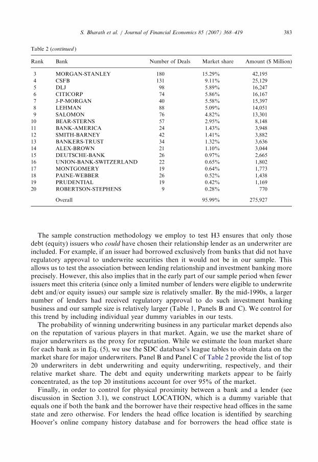
ARTICLE IN PRESS


Rank Bank Number of Deals Market share Amount ($ Million)

3 MORGAN-STANLEY 180 15.29% 42,195

4 CSFB 131 9.11% 25,129

5 DLJ 98 5.89% 16,247

6 CITICORP 74 5.86% 16,167

7 J-P-MORGAN 40 5.58% 15,397

8 LEHMAN 88 5.09% 14,051

9 SALOMON 76 4.82% 13,301

10 BEAR-STERNS 57 2.95% 8,148

11 BANK-AMERICA 24 1.43% 3,948

12 SMITH-BARNEY 42 1.41% 3,882

13 BANKERS-TRUST 34 1.32% 3,636

14 ALEX-BROWN 21 1.10% 3,044

15 DEUTSCHE-BANK 26 0.97% 2,665

16 UNION-BANK-SWITZERLAND 22 0.65% 1,802

17 MONTGOMERY 19 0.64% 1,773

18 PAINE-WEBBER 26 0.52% 1,438

19 PRUDENTIAL 19 0.42% 1,169

20 ROBERTSON-STEPHENS 9 0.28% 770

Overall 95.99% 275,927


The sample construction methodology we employ to test H3 ensures that only thosedebt (equity) issuers who could have chosen their relationship lender as an underwriter areincluded. For example, if an issuer had borrowed exclusively from banks that did not haveregulatory approval to underwrite securities then it would not be in our sample. Thisallows us to test the association between lending relationship and investment banking moreprecisely. However, this also implies that in the early part of our sample period when fewerissuers meet this criteria (since only a limited number of lenders were eligible to underwritedebt and/or equity issues) our sample size is relatively smaller. By the mid-1990s, a largernumber of lenders had received regulatory approval to do such investment bankingbusiness and our sample size is relatively larger (Table 1, Panels B and C). We control forthis trend by including individual year dummy variables in our tests.

The probability of winning underwriting business in any particular market depends alsoon the reputation of various players in that market. Again, we use the market share ofmajor underwriters as the proxy for reputation. While we estimate the loan market sharefor each bank as in Eq. (5), we use the SDC database’s league tables to obtain data on themarket share for major underwriters. Panel B and Panel C of Table 2 provide the list of top20 underwriters in debt underwriting and equity underwriting, respectively, and theirrelative market share. The debt and equity underwriting markets appear to be fairlyconcentrated, as the top 20 institutions account for over 95% of the market.

Finally, in order to control for physical proximity between a bank and a lender (seediscussion in Section 3.1), we construct LOCATION, which is a dummy variable thatequals one if both the bank and the borrower have their respective head offices in the samestate and zero otherwise. For lenders the head office location is identified by searchingHoover’s online company history database and for borrowers the head office state is


identified by searching COMPUSTAT. For non-U.S. banks we search for the U.S.headquarters. For a few Japanese banks we are not able to ascertain the exact location ofU.S. headquarters; for these, we assume that New York is the U.S. head office (we confirmthat all of these banks do have a New York office). For banks that underwent mergers weuse the historical head office for the pre-merger period and the head office of the newmerged entity in the post-merger period.

3.3. Data on characteristics of loan facilities, debt issues and equity issues

We also need to control for various loan characteristics such as maturity, security, andtype of facility. To generate data on loan terms we employ the LPC database. LPCprovides data on a facility-level as well as deal-level basis. A given deal may correspond tomultiple facilities (i.e., multiple loan contracts) of different types of loans to the same firmby one or more banks. Examples of different types of facilities include term loans, lines ofcredit, revolvers, etc. In this study, we use each facility as the unit of observation. Panel Aof Table 3 provides summary statistics on key loan facility terms.The key characteristics for the debt and the equity issues are proceeds raised from the

issue, date of issuance and identity of lead underwriters and co-managers. Our primarysource for these data items, is the SDC new issues database. Panel B of Table 3 reports thesummary statistics for debt issues. We segregate the public equity issues into IPOs andSEOs as the fee structure across these two issue classes is different. Panel C of Table 3provides the summary statistics for equity issues.

3.4. Data on borrower characteristics

Existing theories argue that informational asymmetries between a borrower andpotential debt providers are addressed more effectively by relationship lending than byarms-length financing. Because borrowers that suffer from greater information asymme-tries should gain more from relationship lending, such borrowers are expected to borrowfrom their relationship lender more frequently (see H2). We use different proxies forinformation opacity of a borrower such as borrower size, the loan’s credit rating, and thetangibility of borrower’s assets. COMPUSTAT is our primary data source for borrower-related variables, since the LPC database does not provide a borrower Cusip that can beused as an identifier to match the borrower to other data sets such as COMPUSTAT orCRSP. We therefore manually match the LPC companies with the merged CRSP/COMPUSTAT database using the name of the company in the LPC database. Thematching procedure is conservative in that we assign a match only when we are sure thatthe company is the same in the two databases. Using this procedure, we obtain a set of6,322 borrowers in the LPC database for which we can obtain the Cusip of the companyfrom the COMPUSTAT database. Since a number of borrowers merged or were acquiredby other borrowers over our sample period, we take this M&A activity into account inconstructing our relationship measures. If the post-merger/post-acquisition companyretains the Cusip of one of the predecessor firms, we assume that the relationships of theCusip-retaining firm are inherited by the post-merger/post-acquisition entity while therelationships of the other firm are assumed to be not inherited. Thus, to the extent a post-merger entity also retains the relationships of the target, we underestimate the strengthof the relationship variable. If the merger creates an entity with a new Cusip we follow

ARTICLE IN PRESS

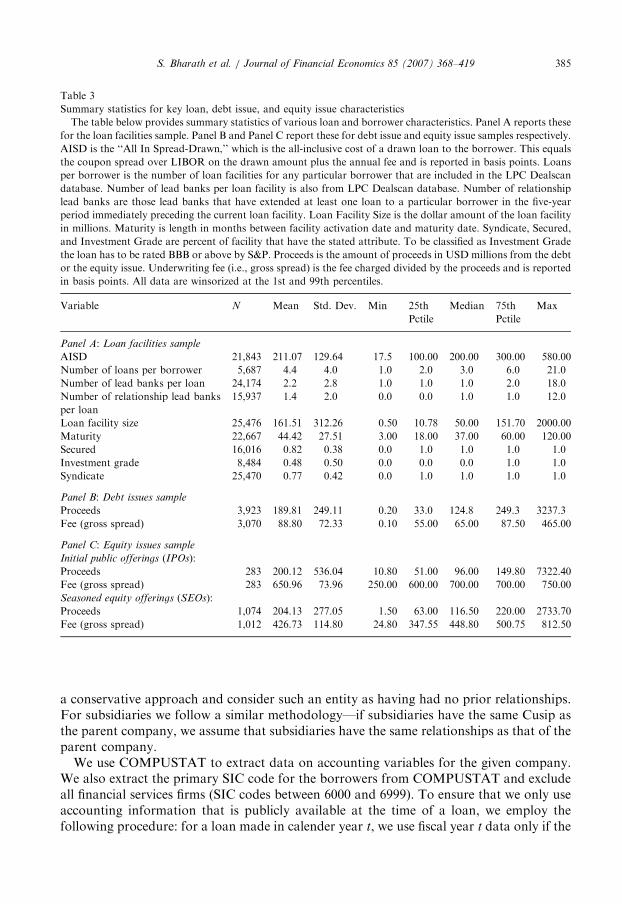
Table 3

Summary statistics for key loan, debt issue, and equity issue characteristics

The table below provides summary statistics of various loan and borrower characteristics. Panel A reports these

for the loan facilities sample. Panel B and Panel C report these for debt issue and equity issue samples respectively.

AISD is the ‘‘All In Spread-Drawn,’’ which is the all-inclusive cost of a drawn loan to the borrower. This equals

the coupon spread over LIBOR on the drawn amount plus the annual fee and is reported in basis points. Loans

per borrower is the number of loan facilities for any particular borrower that are included in the LPC Dealscan

database. Number of lead banks per loan facility is also from LPC Dealscan database. Number of relationship

lead banks are those lead banks that have extended at least one loan to a particular borrower in the five-year

period immediately preceding the current loan facility. Loan Facility Size is the dollar amount of the loan facility

in millions. Maturity is length in months between facility activation date and maturity date. Syndicate, Secured,

and Investment Grade are percent of facility that have the stated attribute. To be classified as Investment Grade

the loan has to be rated BBB or above by S&P. Proceeds is the amount of proceeds in USD millions from the debt

or the equity issue. Underwriting fee (i.e., gross spread) is the fee charged divided by the proceeds and is reported

in basis points. All data are winsorized at the 1st and 99th percentiles.

Variable N Mean Std. Dev. Min 25th

Pctile

Median 75th

Pctile

Max

Panel A: Loan facilities sample

AISD 21,843 211.07 129.64 17.5 100.00 200.00 300.00 580.00

Number of loans per borrower 5,687 4.4 4.0 1.0 2.0 3.0 6.0 21.0

Number of lead banks per loan 24,174 2.2 2.8 1.0 1.0 1.0 2.0 18.0

Number of relationship lead banks

per loan

15,937 1.4 2.0 0.0 0.0 1.0 1.0 12.0

Loan facility size 25,476 161.51 312.26 0.50 10.78 50.00 151.70 2000.00

Maturity 22,667 44.42 27.51 3.00 18.00 37.00 60.00 120.00

Secured 16,016 0.82 0.38 0.0 1.0 1.0 1.0 1.0

Investment grade 8,484 0.48 0.50 0.0 0.0 0.0 1.0 1.0

Syndicate 25,470 0.77 0.42 0.0 1.0 1.0 1.0 1.0

Panel B: Debt issues sample

Proceeds 3,923 189.81 249.11 0.20 33.0 124.8 249.3 3237.3

Fee (gross spread) 3,070 88.80 72.33 0.10 55.00 65.00 87.50 465.00

Panel C: Equity issues sample

Initial public offerings (IPOs):

Proceeds 283 200.12 536.04 10.80 51.00 96.00 149.80 7322.40

Fee (gross spread) 283 650.96 73.96 250.00 600.00 700.00 700.00 750.00

Seasoned equity offerings (SEOs):

Proceeds 1,074 204.13 277.05 1.50 63.00 116.50 220.00 2733.70

Fee (gross spread) 1,012 426.73 114.80 24.80 347.55 448.80 500.75 812.50


a conservative approach and consider such an entity as having had no prior relationships.For subsidiaries we follow a similar methodology—if subsidiaries have the same Cusip asthe parent company, we assume that subsidiaries have the same relationships as that of theparent company.

We use COMPUSTAT to extract data on accounting variables for the given company.We also extract the primary SIC code for the borrowers from COMPUSTAT and excludeall financial services firms (SIC codes between 6000 and 6999). To ensure that we only useaccounting information that is publicly available at the time of a loan, we employ thefollowing procedure: for a loan made in calender year t, we use fiscal year t data only if the


loan activation month is at least six months after the fiscal year-ending month. Otherwise,we use fiscal year t� 1 data.21 The six-month minimum gap between fiscal year-end andthe loan activation date is conservative given the SEC requirement that accounting data bemade available within 90 days of the fiscal year-end. However, compliance with thisrequirement is patchy. Fama and French (1992) state that ‘‘on average 19.8% do notcomply (with this requirement).’’22

4. Methodology and empirical results

In this section we describe the tests we employ to estimate the hypothesized (highervolume) benefits of relationships to lenders (Hypotheses H1, H2 and H3).

4.1. Tests of Hypothesis 1

As we discuss in Section 2, existing theories of relationship lending predict that strongrelationships should be associated with a lower cost of information production over time,provided this information is proprietary and reusable. A testable implication of thesetheories is that a relationship lender is more likely to secure the future lending business ofits borrower. We formalize this implication in our Hypothesis 1. To test this, for each loanfacility we focus on any bank m’s likelihood of winning the loan business of borrower i attime t.While the number of lenders that appear in our sample is quite large (see Table 2), a

handful of banks account for the bulk of lending. To economize on the size of the data setbut still retain most of the large transactions, we choose the following approach. In eachyear, we keep only those transactions for which one of the lead banks was ranked in thetop 40 banks by market share in the prior year. That is, we reduce our sample to thosetransactions for which the lead bank(s) was among the top 40 in the previous year. Thisallows us to retain 73% of our original sample as the top 40 banks provide the bulk of allloans.23 For each loan we create a choice set of 40 potential lenders, thereby creating 40loan-bank pairs.24 Since each loan facility generates a cluster of up to 40 loan-bank pairobservations, our data set consists of over 400,000 loan-bank pairs, which is the unit of

21The following examples illustrate this methodology. Walmart contracted a $1.1 billion loan on October 1,

1999. Walmart’s fiscal year ends on January 31 and thus the October loan is more than six months after the month

of the fiscal year-end closing. In this case we use the accounting data for fiscal year ending January 31, 1999. On

the other hand, Walmart took a $1.25 billion loan on May 29, 1995. Since the May loan was less than six months

after the fiscal year-end closing, we use accounting data for the previous fiscal year, i.e., for the year ending

January 31, 1994.22Even for those firms that do comply, a large proportion file on the last allowed day. Alford et al. (1992) report

that more than 40% of firms with a December fiscal year-end file on March 31, thus, the data becomes available

only in April.23Even for the 27% of the original sample that we do not use, a large fraction (20% of the original) is unusable

regardless of this requirement because these loans were made in the early years of our sample period and we do

not have a long enough history to allow codification of their relationship variables. Thus, we only lose 7% of our

sample to the requirement that it must be led by a top 40 bank.24Drucker and Puri (2005) and Ljungqvist et al. (2006) use a similar approach to implement their underwriter

selection models.


observation in the following logit model:25

ðCHOSENÞm ¼ b0 þ b1ðLOANREL(M)BankLoansm Þ þ b2ðLOAN MKT SHAREÞm

þ b3ðLOCATIONÞm þX

bkðCONTROLÞk. ð6Þ

The variables are

�

2

usi2

on

ban2

ðCHOSENÞm: For each loan facility i, we create a dummy variable ðCHOSENÞm, whichtakes the value of one if a bank m was retained as the lead bank for that loantransaction and zero otherwise.26

�
LOANREL(M)BankLoansm : This is the measure of relationship strength constructed bylooking back over five years from the date of the loan facility activation and searchingwhether the bank had a prior lending relationship with this borrower. As we discuss inSection 3.1.1 and Appendix A, we construct three different specifications for thisvariable to measure the strength of relationship for each of the 40 banks in each loan-bank pair. � ðLOAN MKT SHAREÞm: To estimate the probability of winning the loan business by a
particular bank, we need to control for the reputation of that bank in the loan market.We use its market share as a proxy for reputation. If the loan facility was activated inthe year t, (LOAN MKT SHARE)m is the market share of bank m in the prior year,t� 1, calculated as in Eq. (5).
� ðLOCATIONÞm: This variable is a dummy variable that equals one if bank m and the
borrower in a loan-bank pair both have their head offices in the same state and zerootherwise. We include this variable to control for the fact that a borrower may be morelikely to give repeat business to a particular bank due to its physical proximity. Sinceour relationship measure is based on existence and intensity of past interactions, it maybe biased by a non-relationship factor such as the proximity of a borrower to aparticular lender. Including the LOCATION variable controls for the effect of physicalproximity between a borrower and a lender and partially mitigates this possible bias inour relationship measures.
� ðCONTROLÞk: We control for borrower industry (one-digit SIC codes), the stated
purpose of the loan facility, and the year of the loan facility activation with dummyvariables.

A large number of banking mergers and acquisitions took place during our sampleperiod. We assume that in the case of acquisitions the customer relationships of a bankbeing acquired are inherited by the acquiring bank.27 For mergers, the relationships of themerger partners are assumed to be inherited by the new post-merger entity. We also adjustthe market shares to reflect the M&A activity. Appendix C describes these issues in moredetail and also provides an illustrative example.

5Since observations within each cluster may not be independent, we estimate cluster-corrected standard errors

ng the approach suggested by Williams (2000).6Thus, if a bank was the sole lead bank, only the loan-bank pair for this bank would have CHOSEN equal to

e and for the other 39, CHOSEN would be zero. If the loan facility was led by multiple banks, than all the loan-

k pairs corresponding to these banks would have CHOSEN equal one while it would be zero for the rest.7This is one of the objectives of bank mergers and acquisitions.

ARTICLE IN PRESS

Table 4

Impact of lending relationships on probability of getting future lending business

Panel A of this table provides the logit regression estimates of the following equation:

(CHOSEN)m ¼ b0 þ b1(LOANREL(M)BankLoansm Þ þ b2ðLOAN MKT SHAREÞm

þ b3(LOCATION)m þX

bkðCONTROLkÞ.

For each loan facility i we create a choice set of 40 potential lenders, which creates 40 loan-bank pairs. The top 40

commercial banks in the previous year form the consideration set for each firm in the current year. The dependent

variable, ðCHOSENÞm, takes a value of one if a bank m was retained as the lead bank for that loan transaction

and zero otherwise. We use three proxies for relationship: LOANREL(Dummy)BankLoansm (equals one if there is a

relationship with the bank m in the last five years before the current loan and zero otherwise),

LOANREL(Number)BankLoansm (ratio of the number of loans with bank m to the total number of loans of the

firm in the last five years before the current loan), LOANREL(Amount)BankLoansm (ratio of the dollar value of loans

with bank m to the total dollar value of loans of the firm in the last five years before the current loan).

(LOAN MKT SHARE)m is the share of total lending by bank m in the year prior to the year of loan facility i.

ðLOCATIONÞm is a dummy variable that equals one if both bank m and the borrower have their respective head

offices in the same state and zero otherwise. In the panel at the bottom we illustrate the economic impact that

various variables have on the probability of a bank being chosen as the lead lender. We use the specification

estimated in column 1 to estimate the probability of a bank being chosen as the lead lender if all variables except

the variable being examined are held equal to their mean. We then estimate the predicted probability as the

variable being examined goes from zero to one (except for LOAN MKT SHARE, which is varied from 1%

market share (approximately lowest market share of a top 20 lender) to 10% market share (approximately highest

market share of a top 20 lender)). For example, the first row reports the predicted probability of a bank

being chosen as a lead lender if it did not have a past lending relationship with a borrower

(LOANREL(Dummy)BankLoans ¼ 0Þ and if all other variables are assumed equal to their means. The next row

reports the predicted probability of being chosen if the bank did have a past lending relationship

(LOANREL(Dummy)BankLoans ¼ 1Þ, again holding all else constant at their means. The third row reports the

increase in the predicted probability of being chosen as the lead lender for a relationship lender compared to a

lender with no prior relationship. Panel B reports the results for a number of alternative specifications of the

model estimated in Panel A. Column 1 repeats the analysis in Panel A but uses individual loan deals as the unit of

analysis instead of loan facilities. Column 2 provides a control for loan facilities that are renewals of existing

facilities-RENEWAL equals one if LPC classifies a facility as a refinancing and zero otherwise. Column 3 uses an

alternative measure of lending relationship, MOST RECENT LENDER, which equals one if a bank m was the

lead bank on the most recent loan facility preceding the current facility and zero otherwise. Column 4 uses the

market share of banks in the borrower’s industry, INDUSTRY LOAN MKT SHAREm, which is the share of

loans made to that borrower’s industry by bank m in the year preceding the current loan. Finally in Column 5 we

control for any pricing effects that could affect the lender selection by imputing the loan spreads that banks that

were not chosen may have charged had they been selected. This is denoted by IMPUTED LOAN SPREAD and is

estimated using the Expectation-Maximization (EM) algorithm. Numbers in parentheses are standard errors

corrected for heteroskedasticity and clustering (�� significant at the 1% level, �� significant at the 5% level,� significant at the 10% level).

(1) (2) (3)

Panel A

Const. �3:53�� 2:94�� 3:32��

(.41) (0.4) (0.42)

LOANREL(Dummy)BankLoansm3:27��

(0.03)

LOANREL(Number)BankLoansm4:59��

(0.04)

LOANREL(Amount)BankLoansm4:23��

(0.04)

ðLOAN MKT SHAREÞm 12:23�� 11:37�� 11:32��

(0.21) (0.21) (0.22)

ðLOCATIONÞm 0:38�� 0:44�� 0:39��

(0.05) (0.05) (0.05)


ARTICLE IN PRESS

Industry dummies Yes Yes Yes

Year dummies Yes Yes Yes

Loan purpose dummies Yes Yes Yes

Number of observations 416,239 416,239 416,239

Pseudo R2 0.32 0.31 0.32

Impact of past lending relationships on the probability of being chosen as the

lead lender using the column 1 specification

Probability of being chosen ð%Þ

LOANREL(Dummy)BankLoansm ¼ 0 2.73


Increase in probability 39.73

ðLOAN MKT SHAREÞm ¼ 1% 3.16

ðLOAN MKT SHAREÞm ¼ 10% 8.93


ðLOCATIONÞm ¼ 0 3.54

ðLOCATIONÞm ¼ 1 5.08


(1) (2) (3) (4) (5)

Panel B

Const. �4:36�� 3:52�� 3:40�� 3:28�� 2:49��

(0.39) (0.41) (0.43) (0.65) (0.41)

LOANREL(Dummy)BankLoansm3:27�� 3:23�� 3:16�� 3:05��

(0.03) (0.03) (0.03) (0.03)

RENEWAL �0:10�

(0.06)

LOANREL(Dummy)BankLoansm �RENEWAL 0:31��

(.08)

ðMOST RECENT LENDERÞm 3:41��

(0.03)

ðLOAN MKT SHAREÞm 12:56�� 12:25�� 13:03�� 12:92��

(0.25) (0.21) (0.21) (0.25)

ðINDUSTRY LOAN MKT SHAREÞm 5:93��

(0.14)

ðLOCATIONÞm 0:37�� 0:38�� 0:52�� 0:31�� 0:39��

(.06) (0.05) (0.05) (0.05) (0.06)

ðIMPUTED LOAN SPREADÞm �0:001��

(.0003)

Industry dummies Yes Yes Yes Yes Yes

Year dummies Yes Yes Yes Yes Yes

Loan purpose dummies Yes Yes Yes Yes Yes

Number of observations 288,500 416,239 413,300 230,088 249,440

PseudoR2 0.32 0.32 0.30 0.31 0.30


lead lender using the column 1 specification (Deal basis)






(1) (2) (3)



Panel A of Table 4 reports the results for logit tests of H1. The three columns report theresults for different proxies of lending relationship. The coefficient for all specifications ofpast lending relationships is positive and significant at the 1% level. The panel at thebottom of the table illustrates the economic significance of past lending relationships onthe probability of being chosen to provide future loans. We use the model estimated incolumn (1), where the past lending relationship is captured simply by the existence or lackof prior lending by the same bank in the last five years to calculate these probabilities.28

The predicted probability of a bank being chosen as the lender for a loan facility if it didnot have a past lending relationship (i.e., LOANRELðDummyÞBankLoans ¼ 0), holding allother variables constant at their respective means, is 2.73% (bottom panel, first row).When we recalculate the predicted probability keeping all else the same but changingLOANRELðDummyÞBankLoans ¼ 1, the predicted probability of being chosen for arelationship lender rises to 42.46%.29 Thus, holding all else equal, a bank’s probabilityof being chosen to provide a loan is increased by 39.73% if it had a past lendingrelationship in the prior five years. These results are equally strong if we use continuousmeasures (specifications in columns 2 and 3) that take into account both the existenceand intensity of past lending relationships. For example, changing theLOANRELðNumberÞBankLoans measure from its minimum value of zero to its maximumvalue of one increases the probability of being chosen from 3% to 77%, while forLOANRELðAmountÞBankLoans this probability is predicted to increase from 3% to 69%.30

It is important to highlight that other variables have a predicted and significant impacton the probability of a bank being retained to provide future loans but their economicimpact is smaller compared to the existence of prior lending relationships. As expected,past market share is strongly associated with the ability to win a particular loan mandate.The coefficients for LOAN MKT SHARE and LOCATION are positive and significant atthe 1% level across all specifications. The bottom panel reports the economicinterpretation of these results. As reported in Table 2, the top-ranked lender (Citicorp)had approximately a 10% share of the loan market over our sample period, while the 20th-ranked bank (Wachovia) had approximately a 1% market share. To illustrate the impactof a lender’s reputation on its probability of being retained, we calculate predictedprobability by first keeping LOAN MKT SHARE equal to 1% and then changing it to10%, while all other variables are kept constant at their respective means. The effect of thisis to increase the probability of being chosen from 3% to 9%. Similar calculations showthat the probability of being chosen for a lender that does not have its head office in thesame state as the borrower’s head office ðLOCATION ¼ 0Þ is 3.54% and increases to5.08% if both lender and borrower are located in the same state ðLOCATION ¼ 1Þ.

28To test the power of our specification, we estimate the predicted probabilities for each loan-bank pair

observation by fitting our model to the data. If this predicted probability is greater than 0.5, we assign the bank to

the chosen group and if it is less than 0.5 we assign it to the not-chosen group. Our model predicts the correct

outcome for 93.80% of the observations.29An alternative approach is to interpret the coefficients in terms of an increase in odds ratio. The logit model

for a binary dependent variable Y can be written in terms of the odds that Y would equal 1 as ProbðY¼1Þ1�ProbðY¼1Þ ¼ eðb

0xÞ.

Thus, the odds of being chosen as a lender as a function of prior lending relationship isProbððCHOSENÞm¼1Þ

1�ProbððCHOSENÞm¼1Þ¼ eðb0þb1ðLOANRELðDummyÞBankLoansÞþ

Pbotherðother variablesÞÞ. The coefficient of 3.27 for

LOANRELðDummyÞBankLoans implies that the odds of being chosen as the lender is e3:27, or approximately 26

times higher if a lender had a prior relationship compared to if it did not have a prior relationship.30These results are available from the authors on request.


Again, while significant, this is a much smaller economic effect compared to the oneassociated with having (or not having) a past lending relationship. These results suggestthat establishing a lending relationship with a borrower confers significant economicbenefits upon a lender in terms of a higher probability of securing the future lendingbusiness of that borrower.

4.2. Robustness checks of Hypothesis 1 and other issues

4.2.1. Facilities vs. deals

In Panel B of Table 4 we report results for alternative specifications of lender choicemodel in Eq. (6) so as to verify the robustness of the results reported above to analternative definition of ‘‘loan business.’’31 Specifically, we conduct our analysis on anindividual loan facility basis, i.e., we treat each loan facility, including those that are partof the same deal, as new loan business. While this treatment is likely to have a limitedeffect, since over 70% of the deals in our sample are single loan facility deals, it can stillinflate our relationship results since a lender gets multiple ‘‘credits’’ for winning themandate for a deal that consists of multiple facilities. To examine this issue, we hand-match each loan facility to the original deal and re estimate our relationship measures on adeal-by-deal basis. We report the results in column 1 of Panel B, Table 4. The coefficientfor the LOANRELðDummyÞBankLoans is essentially unchanged at 3.27 compared to theoriginal facility-basis specification and is significant at the 1% level. The economicsignificance continues to be high as well: on a deal-by-deal basis, a bank with aprior lending relationship has a 40.52% probability of getting a future loan dealcompared to 2.51% for a bank that lacks such past relationships. The results forLOANRELðNumberÞBankLoans and LOANRELðAmountÞBankLoans are very similar and areomitted to conserve space.

4.2.2. Renewals vs. non-renewals

Another potential issue is whether a loan facility is a new loan or a renewal of anexisting facility. For example, a borrower may simply be renewing a revolving line of creditthat was part of a deal with a long-maturity loan. In such a case our tests would treatsuch a renewal as equivalent to winning new loan business. Thus, our test would attributewinning such renewals to a past relationship although it is simply a continuation of aprior loan. To address this concern we check the LPC database to determine whethera particular facility was a renewal. We create the variable RENEWAL, which equalsone for a particular facility if the LPC recorded that facility as refinancing, and zerootherwise, and include both RENEWAL and the interaction RENEWAL�LOANREL(Dummy)BankLoans in our logit model. As expected, the results which wereport in column 2, Panel B, show that conditional on a loan being a renewal,past relationships significantly increase the likelihood of winning such a renewalfacility (coefficient for the interaction term is positive and significant at the 1%level). Moreover, even after controlling for renewals, the coefficient forLOANREL(Dummy)BankLoans remains essentially unchanged and continues to be positiveand significant at the 1% level.

31We thank the referee for pointing out the issues discussed below and for suggesting the tests to address them.


4.2.3. Syndication among few dominant banks

Given that a limited number of banks dominate the syndicated loan market(a significant proportion of the LPC loans are syndicated loans), it is possible thatborrowers are simply rotating their lending business among relatively few banks. If this isthe case, these dominant banks would be classified as relationship banks for mostborrowers according to our methodology. The association between past lending and a highprobability of winning future business that we report in Panel A of Table 4 would thensimply be due to syndicate rotation among banks. To address this issue we construct analternative measure of lending relationships, MOST RECENT LENDER, which equalsone if a particular bank was the lead bank on the most recent loan (prior to the currentloan), and zero otherwise. This definition implies that if borrowers are simply rotating theirloan business rather than rewarding relationships, MOST RECENT LENDER shouldhave a negative coefficient (since rotation implies switching lenders after each loan).However, if future loan business is associated with strong lending relationships then theMOST RECENT LENDER variable should have a positive coefficient. As we report incolumn 3, this variable has a coefficient of 3.41 (significant at the 1% level), which is ofsimilar magnitude to the LOANREL(Dummy)BankLoans variable in Panel A. This result isconsistent with the argument that lending relationships are associated with a higherlikelihood of winning future lending opportunities.

4.2.4. Lender characteristics

A further issue pertains to individual lender characteristics. While we control for thephysical proximity and lender reputation of each bank, it is possible that a bank mayacquire a very strong reputation for expertise in lending to a certain industry, e.g., chemicalindustry. In such a case, borrowers in that industry would prefer to borrow from that bankindependent of past relationships. To control for ‘‘industry lending expertise,’’ weconstruct lending market shares of each bank for all the major industry sectors ofborrowers in our sample (these market shares are constructed for each year for every two-digit industry group for which LPC reports at least 10 loans made in that year). For anybank m this is denoted by INDUSTRY LOAN MKT SHAREm. We reestimate our logitmodel by using each bank’s lagged industry loan market share for that borrower’sindustry. The results in column 4 show that the coefficient for lagged industry market shareis 5.93 and is significant at the 1% level. Thus, having large lending market share to aparticular borrower’s industry increases the likelihood of winning future loan business.Even after controlling for such industry expertise the coefficient for theLOANREL(Dummy)BankLoans is 3.16 (significant at the 1% level), which is similar to thecoefficient we estimate in the original specification.

4.2.5. Loan pricing effects

Finally, we address the issue of controlling for loan pricing effects when a borrowerchooses its lender. If the relationship lender also offers the lowest interest rate (measuredby all-in-spread drawn or (AISD)), it is even more likely to win lending business.32 Thus,part of the effect we attribute to relationships may be due in part to a lower price of therelationship loan. However, we cannot directly control for the price charged for a loan in

32AISD measures the interest rate spread on a loan (over LIBOR) plus any associated fees in originating

the loan.


our logit model since we only observe the actual AISD charged by the bank that waschosen, i.e., data are missing for the other ‘‘potential’’ lenders in the choice set that were not

chosen. We address this issue by imputing the loan price for other banks in the choice setthat were not chosen using the expectation–maximization (EM) algorithm as suggested byYasuda (2005).33

The EM algorithm is a general technique for finding the maximum-likelihood estimatesfor parametric models when data are not fully observed. In our context, the principalmissing variable of interest is the rate charged (AISD) by the banks that are not retained ina given loan facility. We use the observed data on AISD and other borrower- and loan-specific characteristics to construct the following model:

(AISD)im ¼ b0 þ b1LOANREL(Dummy)m þ b2(LOAN MKT SHARE)m

þX

bi(LOAN_CHARACTERSTICS)i

þX

bjðBORROWER_CHARACTERSTICSÞj

þX

bkðCONTROLkÞ.

Thus, for a loan i by borrower j, if bank m was chosen the AISDm is the actual observed pricecharged for the loan, and if bank m was not chosen the value for AISDm is set to missing.

The loan characteristics we use are:

�

3

LN(LOAN SIZE): natural log of loan facility amount.
� MATURITY: maturity of loan facility in months. � SYNDICATE: equals one if the loan facility was syndicated, and zero otherwise. � SECURED: equals one if the loan facility was secured, and zero otherwise.
The borrower specific characteristics are:

�
LN(ASSET): natural log of the book value of the assets of the borrower. � LEVERAGE: ratio of the book value of total debt to the book value of assets.� � � COVERAGE: natural log of the ratio 1þ EBITDA
Interest Expenses.

�
PROFITABILITY: ratio of EBITDA to Sales. � TANGIBILITY: ratio of net property, plant, and equipment (NPPE) to the book value
of assets.
� CURRENT RATIO: ratio of current assets to current liabilities. � MARKET TO BOOK: ratio of (book value of assets �book value of equityþmarket
value of equity) to the book value of assets.
� R&D TO SALES: ratio of research and development expenses to sales.
The other control variables include dummy variables for the year and reported purposeand type of the loan facility, the credit rating of the borrower, and the industry of theborrower (two-digit SIC codes).

Each iteration of the algorithm consists of two steps, an expectation step (E step) and amaximization step (M step). The E step involves finding the conditional expectation of themissing data given the observed data and current estimated parameters (or initial estimated

3See Dempster et al. (1977) and McLachlan and Krishan (1997) for good surveys of EM methods.


parameters). Thus, the E step can be thought of as filling in the missing data. Theparameter estimates for the complete data set are then computed in the M Step by usingmaximum likelihood estimation. This process is repeated iteratively until convergenceobtains.This procedure allows us to estimate loan prices that a given bank would have charged if

it had been chosen. We call this variable IMPUTED LOAN SPREAD. We then reestimateour original logit model in Eq. (6) including the IMPUTED LOAN SPREAD for eachpotential lending bank. We present the results of this analysis in the last column of Table 4,Panel B. As expected, the coefficient for IMPUTED LOAN SPREAD is negative andsignificant, implying higher spreads charged make it less likely that the bank would bechosen to provide the loan. The relationship variable, however, continues to be significantand is essentially unchanged.34

4.2.6. Modeling the lender selection process

In our lender choice model we allow up to 40 banks as possible choices to a borrower.This borrower choice set may include a number of banks that potentially did not bid forthe business and thus our results may overstate the importance of relationships. To addressthis concern we carry out a number of robustness checks.35

First we model the selection of a particular bank as a two-stage decision. In the firststage the borrower decides whether to use a relationship borrower or not and in the secondstage it chooses a specific bank conditional on its propensity to choose relationship banks.We construct a binary variable REL for each loan facility; REL equals one if at least oneof the lenders chosen had been a lender in the previous five years. We model the choicebetween a relationship and non-relationship loan as a function of various loan andborrower characteristics. These include loan size, credit rating, borrower size, profitability,leverage, and a specific measure that captures the intensity of using relationship lenders inthe past. We estimate this past usage of relationship banks by calculating the fraction of allprior loans in which relationship lenders were used. This model allows us to estimate thepredicted probability of using relationship lenders for each loan, which we denote bydPROBREL. In the second stage we focus on specific lender characteristics that determinethe choice of a particular lender after controlling for the borrower’s propensity to chooserelationship lenders. Specifically, we estimate a modified version Eq. (6) in which weinclude dPROBREL as another explanatory variable. This second-stage estimation allowsus to measure the impact of prior relationships that a specific bank m has after controllingfor that borrower’s propensity to use relationship lenders in general. The coefficient forLOANREL(Dummy) in the second-stage regression is 3.09, which is significant at the 1%level and similar to the coefficient of 3.27 as reported in the original specification (column 1of Panel A, Table 4). Thus, even after controlling for a particular borrower’s propensity touse relationship lenders, the prior relationship that a specific lender has is significantlyassociated with that lender’s ability to win future lending business.

34We also use an alternative method suggested by Schafer (1997) whereby we simulate 100 random data sets for

loan spreads based on the observed distributions of spreads and other independent variables. For each of these

samples, we estimate the effect of bank’s market share and relationships on loan prices. We use the average

estimates from these 100 simulations to calculate imputed fees for a given transaction for each bank-transaction

pair. The results from using imputed loan spreads obtained from this simulation- based approach are similar to

those estimated by using the EM algorithm.35The results for these tests are not reported but are available from authors on request.


We also reestimate our model with smaller choice set of potential lenders for each loanfacility. First we reduce the potential choice of lenders for each loan facility to top 20banks (as ranked by market share in the previous year). This smaller choice set makes itmore likely that all the lenders were potential bidders for the loan. This choice set size isalso similar to that used by Drucker and Puri (2005), who use a choice set of 20, andYasuda (2005), who uses a choice set of 16. The coefficient for LOANREL(Dummy) is3.17 (significant at the 1% level), which is very similar to that for the original specification.We also rerun our model by restricting the choice set to the top 10 lenders. The coefficientof LOANREL(Dummy) remains essentially unchanged at 3.15, significant at the 1% level.Finally, we restrict the choice set of lenders for each borrower to top 10 lenders in theborrower’s industry (defined at the two-digit SIC code level). The coefficient forLOANREL(Dummy) is 3.14 and significant at the 1% level. These results imply thatour findings of a prior lending relationship having a significant impact on the ability to winfuture lending business is not driven by the size of the choice set used.

Finally, we construct a subset of borrowers for which key requirements forimplementing the nested logit model hold.36 We construct a subsample of borrowers,which, when faced with a lender selection decision, could have either chosen one of its tworelationship borrowers or one of the 37 non-relationship borrowers. These restrictionsyield a subsample of 13,416 observations. At the upper level a borrower chooses betweenthe relationship and non-relationship nest. At the lower level it chooses a specific lender.We model the first-stage decision as largely determined by borrower characteristics and thelower-level decision to be based on specific lender characteristics such as market share,location, and whether it was the lead bank for the most recent loan (denoted by MOSTRECENT LENDER). We find that the coefficient for MOST RECENT LENDER ispositive and significant at the 1% level. Thus, even after conditioning for a borrowerchoosing a relationship lender, the lender that provided that most recent loan has asignificantly higher probability of winning the next loan.

Overall, the robustness tests we employ above suggest that past lending relationships aresignificantly and positively associated with future lending opportunities.

4.3. Tests for Hypothesis 2

Theoretical models (e.g., Diamond, 1991) predict that relationships are more beneficialfor firms that suffer from greater informational asymmetries. This motivates ourHypothesis 2, which conjectures that informationally opaque firms use relationshiplenders more frequently. To test this we use different proxies for information‘‘opaqueness,’’ specifically, the borrower’s size and the borrower’s credit rating (seeSections 4.3.1 and 4.3.2 below). We also report results for alternative proxies forborrower’s information opaqueness in Section 4.3.3.

4.3.1. The effect of borrower size and Hypothesis 2

A priori, it is reasonable to argue that smaller-sized firms are less likely to be widelyfollowed by either capital market investors (or credit rating agencies). Stein (2002) arguesthat small-business lending ‘‘relies heavily on information that is soft—that is, information

36These requirements entail that all borrowers face exactly the same number of choices in both the relationship

nest and the non-relationship nests, and that each borrower chooses exactly one lender.


that cannot be verified by anyone other than the agent who produces it.’’ Thischaracterization suggests that smaller borrowers should find strong relationships withtheir lenders particularly beneficial. Smaller firms are also likely to be relatively moreinformationally opaque; for example, Petersen and Rajan (1994) state that ‘‘. . . there maybe large information asymmetries between these [small] firms and potential publicinvestors.’’37 Thus, small firms offer the most potential for proprietary informationgeneration by a relationship lender. To the extent that relationships do mitigate theinformation problems that smaller firms face, we should expect to find a strong associationbetween the size of a borrower and its use of a relationship bank for future loans.To examine if relationship lending varies across different borrower sizes, we divide our

sample into three size terciles based on borrower’s book value of assets. Specifically, weadd the two dummy variables MIDDLE and BIG to Eq. (6). These variables equal one ifthe borrower falls in the stated size tercile and zero otherwise. We also add two interactionterms, multiplying the relationship variable with MIDDLE and BIG. The modified logitmodel is then


þ b3ðLOCATIONÞm þ b4ðMIDDLEÞ þ b5ðBIGÞ

þ b6ðMIDDLE � LOANREL(M)BankLoansm Þ

þ b7ðBIG � LOANREL(M)BankLoansm Þ þX

bkðCONTROLkÞ. ð7Þ

The results, in Table 5, Panel A, describe how past lending relationships affect theprobability of winning future lending business across different-sized borrowers. Sincelarger borrowers are likely to be informationally more transparent, holding everything elseconstant the effect of past relationships on the probability of being chosen as a lendershould be the weakest for the large borrowers and the strongest for small borrowers. Thecoefficient of LOANRELðDummyÞBankLoansm is 5.01 if the borrower is in the smallest sizetercile, 4.13 for the middle tercile and 3.71 for the largest tercile, even as it continues to bestatistically significant across all borrower size terciles (Table 5, column 1). Thus, the effectof past relationships, while significant, declines as one goes from the smallest borrowers tothe largest borrowers. This is also captured in the negative coefficient of the size andrelationship interaction terms, which are negative and significant at the 1% level across allspecifications. In the panel at the bottom of Table 5 we use the specification estimated incolumn 1 to illustrate the economic significance of past lending relationship benefits acrossdifferent borrower size terciles. Specifically, we estimate the probability of a bank beingchosen as the lead lender if all variables except the relationship variables and the sizevariables are held equal to their means. The impact of a past relationship on theprobability of being chosen as lead lender is measured by setting each specific size variableequal to one while keeping the other size variables equal to zero. The first row reports thepredicted probabilities (for borrowers in small, medium, and large terciles) of a bank beingchosen as a lead lender if it did not have a past lending relationship with a borrower(LOANRELðDummyÞBankLoansm ¼ 0) and if all other variables are assumed to be equal totheir means. The next row reports the predicted probability of being chosen if the bank didhave a past lending relationship (LOANRELðDummyÞBankLoansm ¼ 1). We find that having

37A number of empirical studies use smaller borrower size as proxy for higher information asymmetries. See, for

example, Blackwell and Kidwell (1988) and Houston and Christopher (1996).

ARTICLE IN PRESS

Table 5

Borrower information asymmetries, lending relationships and probability of getting future lending business

Panel A of this table provides the logit regression estimates of the following equation:

ðCHOSENÞm ¼ b0 þ b1ðLOANREL(M)BankLoansm Þ þ b2ðLOAN MKT SHAREÞm þ b3ðLOCATIONÞm

þ b4ðMIDDLEÞ þ b5ðBIGÞ þ b6ðMIDDLE * LOANREL(M)BankLoansm Þ

þ b7ðBIG � LOANREL(M)BankLoansm Þ þX

bkðCONTROLkÞ.

The model is the same as one we estimate in Table 4 with except here we include, two dummy variables, MIDDLE

and BIG, which take the value one if the borrower falls in the stated size tercile (as measured by the book value of

assets) and zero otherwise. We also add two interaction terms, multiplying the relationship variables with

MIDDLE and BIG.

Panel B reports the estimates of the following logit regression:


þ b4ðNOT RATEDÞ þ b5ðNOT RATED � LOANREL(M)BankLoansm Þ

þX

bkðCONTROLkÞ.

Again, the model is the same as the one we estimate in Table 4 except we add an additional variable NOT RATED

(and the interaction with relationship measures), which equals one if the loan is not rated and zero otherwise.

Panel C provides estimates the following logit regression:


þ b4ðINVESTMENT GRADEÞ þ b5ðINVESTMENT GRADE*(LOANREL(M)BankLoansm Þ

þX

bkðCONTROLkÞ.

The model is the same as the one we estimate in Table 4 except we add an additional variable INVESTMENT

GRADE (and the interaction with relationship measures), which equals one if the loan is rated BBB or above by

S&P and zero otherwise.

At the bottom of each panel we illustrate the economic impact of past lending relationships on the probability

of being chosen as the lead lender (across borrowers with different levels of information opacity) using the

specification estimated in column 1. Specifically, we estimate the probability of a bank being chosen as the lead

lender if all variables except the relationship variables and the information opacity measure (size, credit rating,

etc.) are held equal to their means. Then the impact of a past relationship on the probability of being chosen is

measured across different information opacity measures for each size tercile (e.g., by setting each size variable

equal to one while keeping the other size variables equal to zero). Numbers in parentheses are standard errors

corrected for heteroskedasticity and clustering (�� significant at the 1% level, �� significant at the 5% level,� significant at the 10% level).

(1) (2) (3)

Panel A: Borrower size and relationship lending

Const. �4:45�� 4:01�� 4:30��

(0.39) (0.38) (0.40)


ð0:09Þ


ð0:13Þ


(0.12)


(0.21) (0.22) (0.22)

ðLOCATIONÞm 0:36�� 0:44�� 0:38��

(0.05) (0.05) (0.05)

MIDDLE 0:37�� 0:41�� 0:39��

(0.05) (0.05) (0.05)

BIG 1:26�� 1:34�� 1:31��

(0.05) (0.05) (0.05)


ARTICLE IN PRESS

MIDDLE� LOANREL(Dummy)BankLoansm�0:88��

(0.1)

BIG� LOANREL(Dummy)BankLoansm�2:30��

(0.10)

MIDDLE� LOANREL(Number)BankLoansm�0:56��

(0.15)

BIG� LOANREL(Number)BankLoansm�1:89��

(0.14)

MIDDLE� LOANREL(Amount)BankLoansm�0:59��

(0.13)

BIG� LOANREL(Amount)BankLoansm�2:07��

(0.13)





Pseudo R2 0.33 0.32 0.33



Probability of being chosen

Small ð%Þ Medium ð%Þ Big ð%Þ

LOANREL(Dummy)BankLoansm ¼ 0 1.21 1.74 4.14

LOANREL(Dummy)BankLoansm ¼ 1 64.87 52.24 39.28

Increase in probability 63.66 50.50 35.14

Panel B: Availability of borrower credit rating and relationship lending

Const. �3:20�� 2:57�� 2:97��

(0.39) (0.38) (0.41)


(0.03)


(0.06)


(0.05)


(.21) (0.22) (0.22)

ðLOCATIONÞm 0:37�� 0:45�� 0:39��

(0.05) (0.05) (0.05)

NOT RATED �0:70�� 0:70�� 0:69��

(0.04) (0.03) (0.04)

NOT RATED� LOANREL(Dummy)BankLoansm1:12��

(0.06)

NOT RATED� LOANREL(Number)BankLoansm0:97��

(0.09)

NOT RATED� LOANREL(Amount)BankLoansm1:06��

(0.08)


Table 5 (continued)

(1) (2) (3)


ARTICLE IN PRESS




Pseudo R2 0.32 0.32 0.33




Not rated ð%Þ Rated ð%Þ

LOANREL(Dummy)BankLoansm ¼ 0 1.84 3.66


Increase in probability 48.47 36.40

Panel C: Borrower credit rating and relationship lending

Const. �2:98�� 2:34�� 2:70��

(0.55) (0.53) (0.55)


(0.05)


(0.08)


(0.07)


(0.27) (0.29) (0.29)

ðLOCATIONÞm 0:39�� 0:45�� 0:39��

(0.06) (0.07) (0.07)

INVESTMENT GRADE 0:52�� 0:49�� 0:51��

(.06) (0.05) (0.05)

INVESTMENT GRADE� LOANREL(Dummy)BankLoansm�0:59��

(0.07)

INVESTMENT GRADE� LOANREL(Number)BankLoansm�0:75��

(0.11)

INVESTMENT GRADE� LOANREL(Amount)BankLoansm�0:76��

ð0:10Þ





Pseudo R2 0.30 0.29 0.30




Non investment grade ð%Þ Investment grade ð%Þ



Increase in probability 38.19 34.44

Table 5 (continued)

(1) (2) (3)



a past lending relationship increases the probability of being chosen by 63.7% (from 1.2%to 64.9%) for the borrowers in the smallest tercile. The predicted probability increase forborrowers in the middle and the largest size terciles is 50.5% (1.7% to 52.2%) and 35.2%(from 4.1% to 39.3%), respectively. Thus, the probability of a bank being chosen toprovide future loans gets smaller as borrower size increases.

4.3.2. The effects of credit rating and Hypothesis 2

An alternative proxy for informational asymmetries is the availability of a credit ratingfor the borrower. If the borrower is not rated, a debt-holder needs to generate and processa relatively larger amount of information to make its lending decision. Thus, nonratedborrowers are more likely to turn to their relationship lender for their financing needs thanto public debt markets. For example, Diamond (1991) argues that a borrower’s pastrepayment reputation would drive its choice of borrowing source. A key prediction of hismodel is that firms with good reputations (i.e., with high credit ratings) would be able toissue (cheaper) public debt, while firms with lower reputations (as evidenced by lowercredit ratings) would use bank financing. It is also frequently argued that the informationadvantages of an insider lender (scale economies in information production, better abilityto renegotiate covenants, etc.) would allow it to adopt a more flexible approach towardsdebt renegotiations. Thus, a relationship bank is expected to ‘‘lean against the wind’’ whenits borrowers face financial difficulties.38 Consequently, a borrower with a poor creditrating is more likely to use its relationship bank for its borrowing needs.39 Below, weemploy the existence and level a of credit rating for a borrower as a proxy for theinformation asymmetries that the borrower faces.To do this we first partition our sample into firms that have a credit rating and those that

do not. We use the credit rating of the loan facility being examined (as reported by LPC) asthe most timely measure of the borrower’s credit worthiness. It is reasonable to assumethat, on average, the firms whose loans are not publicly rated, are likely to be lessinformationally transparent relative to those that have a rating. Thus, we estimate themodel


þ b3ðLOCATIONÞm þ b4ðNOT RATEDÞ

þ b5ðNOT RATED � LOANREL(M)BankLoansm Þ

þX


The model in Eq. (8) includes a dummy variable (NOT RATED), which equals one ifthe loan is not rated and zero otherwise. We also add an interaction term that interacts therelationship variable with NOT RATED to better isolate the effect of the availability of acredit rating on the use of a relationship banker for future borrowing.

38Hoshi et al. (1990) provide evidence in support of this view. They report that among the financially distressed

Japanese firms, those with strong banking relationships are better able to maintain their investment programs

compared to firms that lacked such banking relationships.39Anecdotal evidence of the limited benefits of relationship lending to the best quality borrowers is highlighted

in an Economist article dated February 12, 1998, which states: ‘‘. . . Part of [JP] Morgan’s problem is that its

customers are simply too good. The trouble with serving only the best firms is that they typically like to maintain

relationships with at least three banks and play them off against each other to get prices down.’’


For the subsample in which the credit rating of the borrower is available, we estimate themodel


þ b3ðLOCATIONÞm þ b4ðINVESTMENT GRADEÞ

þ b5ðINVESTMENT GRADE � LOANREL(M)BankLoansm Þ

þX

bkðCONTROLkÞ, ð9Þ

where INVESTMENT GRADE is a dummy variable that equals one if the loan is ratedBBB or above by S&P, and zero otherwise. We also add an interaction term that multipliesthe relationship variable with INVESTMENT GRADE to better isolate the effect of creditrating on the use of a relationship banker for future borrowing.

Panel B of Table 5 reports the results of Eq. (8). Consistent with our earlier finding,while the existence of a past relationship increases the probability of winning future loansfor all borrowers, this increase is significantly higher for borrowers whose loans have notbeen rated. Specifically, the coefficient of 3.19 for LOANRELðAmountÞBankLoans if aborrower’s loan does not have a rating is higher compared to the coefficient of 2.87 for theborrowers with a rated loan (Table 5, column 1). The impact of credit ratings is alsocaptured by the positive and significant (t-value ¼ 18:7) coefficient of the interaction term(multiplying past relationship by the availability of a borrower’s credit rating). The bottompanel provides the economic interpretation of these results. For a nonrated borrower, arelationship lender has a 48% higher probability (50% vs. 2%) of winning future lendingbusiness, while for a rated borrower, the existence of past relationships increases thepredicted probability of being chosen for future loans by 36% (40% vs. 4%). As a result,while the likelihood of being retained for future loans is fairly low for non-relationshiplenders to both nonrated (2%) and rated borrowers (4%), the probability of a relationshiplender being retained by a nonrated borrower is 10% higher compared to a rated borrower(50% vs. 40%).

Next, we employ the quality of credit rating as a measure of the informationaltransparency of a borrower as in Eq. (9). Borrowers with an investment grade rating (BBBor above) are classified as INVESTMENT GRADE. As we discuss earlier, theoreticalmodels predict that high quality borrowers gain relatively less from borrowing from theirrelationship lender. Thus, we expect the effect of relationships to be weaker for borrowerswith a high credit rating. The results we report in Table 5, Panel C provide some weaksupport for these predictions. The coefficient on the relationship and investment graderating interaction term is negative and significant at the 1% level across all specifications(t-value range of �6:82 to �8:43). Holding all other variables constant at their means, theexistence of a past lending relationship is associated with a 38% increase (3% to 41%) inthe probability of being retained for borrowers with loans rated below investment grade.For BBB or above borrowers, past relationships increase the probability of being retainedby 34% (5–39%).

4.3.3. Alternative proxies for borrower opaqueness

We also employ some alternative proxies for borrower information transparency to testH2.40 In particular, we focus on proxies that measure the tangibility of assets owned by

40To conserve space these results are not reported but are available from the authors upon request.


a firm so as to capture the information asymmetry faced by its lenders. Firms that have arelatively lower fraction of their asset base in tangible assets, such as plant and machinery,face higher information asymmetries and are more likely to use an informed ‘‘insider’’lender for their financing needs. For example, Houston and Christopher (1996) note ‘‘. . .smaller firms and firms with higher proportion of intangible assets (and presumably moredifficult to value assets) are expected to rely primarily on bank financing.’’The first proxy we use is the market-to-book ratio of the borrower, which equals the

ratio of the market value of assets to the book value of assets. The market value iscalculated as the book value of the assets minus the book value of equity plus the marketvalue of equity. Smith and Watts (1992) and Barclay and Smith (1995a, b) use the market-to-book ratio to proxy for the growth options in a firm’s investment opportunity set. Sincea firm’s balance sheet does not include intangible assets such as growth options but itsmarket value reflects such intangible assets, a high market-to-book ratio can be consideredas a firm having a larger fraction of their assets as intangible assets.41 We also employ theratio of Research and Development expenses to Sales as another measure of growthoptions, since a relatively high R&D expenditure could be interpreted as investment inassets that would yield higher future growth. Finally, we also use a ‘‘tangibility ratio,’’calculated as the ratio of net plant, property, and equipment (NPPE) to total assets. Ahigher fraction of total assets in the form of easier-to-value NPPE implies that such firmsface a lower level of informational asymmetry when it comes to raising nonbank debt.This, in turn, implies a lower propensity to use a relationship bank for future financing.For each of these ratios we partition our sample into three ‘‘tangibility’’ terciles and

estimate the impact of lending relationships on these alternative measures of informationopacity. We expect firms with a higher market-to-book ratio, a lower NPPE-to-total assetratio and a higher R&D-to-sales ratio to be more likely to borrow from their relationshiplenders. The results for the market-to-book ratio measure are as predicted. Specifically, thecoefficient for LOANRELðDummyÞBankLoansm is largest (3.27) for the highest tercile(market-to-book) borrowers and smallest (3.13) for the lowest tercile. When we use theR&D-to-sales ratio as a proxy for the borrower’s asset intangibility, we obtain mixedresults. The borrowers in the middle tercile have the highest coefficient (3.72) forLOANRELðDummyÞBankLoansm , with no statistical difference between the lowest and thehighest terciles (3.25 and 3.21, respectively). Using the NPPE-to-total assets ratio as aproxy for the borrower’s asset tangibility, we obtain results in the expected direction, i.e.,borrowers in the highest tercile (borrower’s for which the bulk of their assets are in NPPE),had the lowest coefficient for LOANRELðDummyÞBankLoansm (3.09) while borrowers in thelowest tercile have the highest coefficient (3.39).Taken together our findings in Section 4.3 provide support for the theoretical

predictions underlying H2. That is, informationally opaque firms are more likely to findrelationship borrowing beneficial, than are informationally transparent firms.

4.4. Tests for Hypothesis 3

In Hypothesis 3 we conjecture that if there are scope economies in informationproduction, a relationship lender would have a higher probability of supplying future

41Houston and Christopher (1996) find that for borrowers with multiple banking relationships, those that have

higher market-to-book ratios are more likely to use bank financing.


investment banking and/or underwriting services (i.e., this is the cross-product marketingmotivation behind lending relationships—see, for example, Kanatas and Qi, 2003).

4.4.1. Tests of Hypothesis 3 and debt underwriting

For our empirical tests, we concentrate on two specific investment banking products thata relationship lender can potentially sell to its existing borrower. The first is theunderwriting of public debt issues and the second is the underwriting of public equityissues (IPOs and SEOs).

From the SDC database we obtain details related to all the debt and equity issuescompleted by our sample borrowers, that had at least one relationship lender eligible toprovide the underwriting service (see Section 3.2 for our sample selection methodology).For each issue of public debt in year t (in what follows, the process for equity markets isexactly the same) we construct a choice set of top 20 financial institutions (ranked bymarket share of debt underwriting in the year t� 1). To this set of 20, we add all thecommercial banks that are not in the top 20 list that were eligible to underwrite publicissues of debt at the date of the debt issue.42 To test whether prior lending relationships areassociated with a higher probability of winning an underwriting mandate for issues ofpublic debt, we estimate the following logit model:

ðRETAINÞlead�debtm ¼ b0 þ b1ðPROCEEDSÞ þ b2ðLOANREL(M)PublicDebtm Þ

þ b3ðLead-DEBTREL(M)PublicDebtm Þ

þ b4ðLead-EQUITYREL(M)PublicDebtm Þ

þ b5ðLOAN MKT SHAREÞm þ b6ðTOP TIER-DEBTÞm

þ b7ðMID TIER-DEBTÞm þ b8ðTOP TIER-EQUITYÞm

þ b9ðMID TIER-EQUITYÞm þX


The variables are:

�

4

yea4

on

tha

zer

ðRETAINÞleadm �debt: For each debt issue, we create a dummy variable ðRETAINÞlead�debtm

that takes a value of one if a bank m was retained as the ‘‘Lead Underwriter’’ for thatdebt issue transaction, and zero otherwise.43

�
PROCEEDS: The dollar amount of proceeds from the debt issue in USD millions. � LOANREL(M)PublicDebt
m : The measure of the lending relationship that m has withthe issuer, constructed in exactly the same way as LOANREL(M)BankLoansm exceptthat for LOANREL(M)PublicDebt

m , the date of the look-back period is the date of apublic issue of debt, while for LOANREL(M)BankLoansm , the loan facility activation dateis used.
� Lead-DEBTREL(M)PublicDebt
m and Lead-EQUITYREL (M)PublicDebtm : The relationship

strength measures for debt issue and equity issue markets, respectively. These measurethe intensity of past investment banking relationships of a bank m in debt underwriting

2That is, if it had underwritten (either as lead or as co-manager) at least one debt issue in the years prior to

r t.3Thus, if a bank was the sole underwriter, only the issue-bank pair for this bank would have RETAIN equal to

e and for the other members of the choice set RETAIN would be zero. If the issue were led by multiple banks,

n all the issue-bank pairs corresponding to these banks would have RETAIN equal one while it would equal

o for the rest.

ARTICLE IN PRESS

4

hav


and equity underwriting markets. The construction of these variables is described inSection 3.1 and Appendix A.
� ðLOAN MKT SHAREÞm: for each bank m, is calculated for the year prior to the year
of the debt issue and is calculated as in Eq. (5).
� ðTOP TIER-DEBTÞm: a dummy variable equal to one if the bank m is ranked in the top
5 debt underwriters in the previous year, and zero otherwise.
� ðMID TIER-DEBTÞm: a dummy variable equal to one if the bank m is ranked from 6th
to 15th in debt underwriting in the previous year, and zero otherwise.
� ðTOP TIER-EQUITYÞm: a dummy variable equal to one if the bank m is ranked in the
top 5 equity underwriters in the previous year, and zero otherwise.
� ðMID TIER-EQUITYÞm: a dummy variable equal to one if the bank m is ranked from
6th to 15th in equity underwriting in the previous year, and zero otherwise.

We do not include the LOCATION variable for underwriter selection models as mostof the institutions in the choice set of potential underwriters have a New York Cityhead office.The results, reported in Table 6, provide strong support for H3 in the debt issue

underwriting business. In columns 1–3 we report the results for all three alternativemeasures of prior lending and prior investment banking relationship variables and thecontrols for underwriter reputation both in the debt and the equity markets (as we describein Eq. (10)). The coefficient for LOANREL(M)PublicDebt is positive and significant at the1% level for all specifications.44 Not surprisingly, a prior investment banking relationshipin the same market ðLead-DEBTREL(M)PublicDebt) is a strong determinant of future debtunderwriter selection. The bottom panel, in which we use the model specification describedin column 1 of Table 6 to explore the impact of prior lending and investment bankingrelationships, illustrates the economic significance of prior lending relationships and priordebt underwriting relationships. If all variables are held constant at their means and abank did not have a past lending relationship ðLOANREL(Dummy)PublicDebt

¼ 0Þ with adebt issuer, its probability of being retained as the lead underwriter of that debt issue is0.29%. This probability increases to 0.55% if the bank had a prior lending relationshipðLOANREL(Dummy)PublicDebt

¼ 1Þ with the issuer. While a past lending relationship has astatistically significant impact on the probability of being chosen as the future debtunderwriter, the economic significance (0.55% probability) is, nevertheless, relativelysmall. The economic significance of having a past record of providing (underwriting) thesame product is larger but still economically small, as illustrated by the change inprobability for a bank with and without a prior debt underwriting with the customerrelationship holding all variables constant at their respective means. The existence of aprior debt underwriting relationship increases the probability of winning the leadunderwriter role (from 0.28% for banks with no prior debt underwriting relationship to2.61% for banks with prior debt underwriting relationships). Finally, the existence of apast cross-market investment banking relationship ðLead-EQUITYRELPublicDebt

¼ 1Þ isassociated with an increase in the probability of being retained as lead debt underwriter(0.31% to 0.79%). A prior investment-banking relationship, even in a different productmarket (equity underwriting), has a positive relationship with thelikelihood of winning

4These results are similar to those reported by Yasuda (2005), who also finds that past lending relationships

e a significant impact on winning future debt underwriting mandates.

ARTICLE IN PRESS

Table 6

Impact of lending relationships on probability of getting future debt underwriting business

This table provides the logit regression estimates of the following equation:

ðRETAINÞLead�debtm ¼ b0 þ b1ðPROCEEDSÞ þ b2ðLOANREL(M)PublicDebtm Þ

þ b3ðLead-DEBTREL(M)PublicDebtm Þ

þ b4ðLead-EQUITYREL(M)PublicDebtm Þ þ b5ðLOAN MKT SHAREÞm

þ b6ðTOP TIER-DEBTÞm þ b7ðMID TIER-DEBTÞm

þ b8ðTOP TIER-EQUITYÞm þ b9ðMID TIER-EQUITYÞm þX

bkðCONTROLkÞ.

For each debt issue, we create the dummy variable RETAINLead�debtm , which takes a value of zero if a bank m was

retained as the lead underwriter for that debt issue transaction and zero otherwise. For each debt underwriting

deal i we create a choice set of at least 20 potential underwriters, creating at least 20 deal-underwriter pairs. The

top 20 debt underwriters (based on market share) from the previous year and all commercial banks eligible to do

debt underwriting in the previous year form the consideration set for each issuer in the current year. For each

institution in a transaction-bank pair we estimate relationships across three markets: the bank loan market, the

debt underwriting market, and the equity underwriting market. Within each market we use three different proxies

of relationship strength for any bank m: LOANREL(Dummy)PublicDebtm (one if there is a loan relationship with

bank m in the last five years before the present debt underwriting transaction and zero otherwise),

LOANREL(Number)PublicDebtm (ratio of the number of loan deals with bank m to the total number of loan

deals of the firm in the last five years before the current debt underwriting transaction), and

LOANREL(Amount)PublicDebtm (ratio of the dollar value of loan deals with bank m to the total dollar value of

loan deals of the firm in the last five years before the current debt underwriting transaction).

Lead-DEBTREL(Dummy)PublicDebtm (one if there is a debt underwriting relationship in the lead underwriter

capacity with bank m in the last five years before the present debt underwriting transaction and zero otherwise),

Lead-DEBTREL(Number)PublicDebtm (ratio of the number of debt underwriting deals in the lead underwriter

capacity with bank m to the total number of debt underwriting deals of the firm in the last five years before the

current debt underwriting transaction), and Lead-DEBTREL(Amount)PublicDebtm (ratio of the dollar value of debt

underwriting deals in the lead underwriter capacity with bank m to the total dollar value of debt underwriting

deals of the firm in the last five years before the current debt underwriting transaction).

Lead-EQUITYREL(Dummy)PublicDebtm (one if there is an equity underwriting relationship in the lead underwriter

capacity with bank m in the last five years before the present debt underwriting transaction and zero otherwise),

Lead-EQUITYREL(Number)PublicDebtm (ratio of number of the equity underwriting deals in the lead underwriter

capacity with bank m to the total number of equity underwriting deals of the firm in the last five years before the

current debt underwriting transaction), and Lead-EQUITYREL(Amount)PublicDebtm (ratio of the dollar value of

equity underwriting deals in the lead underwriter capacity with bank m to the total dollar value of equity

underwriting deals of the firm in the last five years before the current debt underwriting transaction). PROCEEDS

is the amount raised in USD millions for the debt underwriting transaction (reported coefficient has been divided

by 1,000). ðLOAN MKT SHAREÞm is the market share of bank m in the loan market in the year before the

current debt underwriting transaction. Similar calculations estimate market shares for the debt underwriting and

the equity underwriting markets. ðTOP TIER-DEBTÞm and ðTOP TIER-EQUITYÞm are dummy variables that

equals one if the bank m is ranked in the top five debt and equity underwriters, respectively, and zero otherwise.

ðMID TIER-DEBTÞm and ðMID TIER-EQUITYÞm are dummy variables that equals one if the bank m is ranked

from 6th to 15th in debt and equity underwriting, respectively, and zero otherwise. ðCOMMERCIAL BANKÞm is

a dummy variable that equals one if bank m had a Section 20 and/or investment banking subsidiary that was

eligible to underwrite debt securities on the date of issuance and zero otherwise.

At the bottom of each panel we illustrate the economic impact of past lending, debt underwriting, and equity

underwriting relationships on the probability of being chosen as the debt underwriter using the specification

estimated in column 1. The first row reports the probability of a non-relationship bank

ðLOANREL(Number)PublicDebt¼ 0Þ being chosen as the debt underwriter if all other variables are held equal

to their mean. The second row reports the probability for a relationship bank ðLOANREL(Number)PublicDebt¼ 1Þ

in the same way. Numbers in parentheses are standard errors corrected for heteroskedasticity and clustering

(�� significant at the 1% level, �� significant at the 5% level, � significant at the 10% level).


ARTICLE IN PRESS

(1) (2) (3) (4) (5)

Const. �6:27�� 7:06�� 6:98�� 5:96�� 6:27��

(.20) (.18) (.17) (.35) (.20)

PROCEEDS 0:34�� 0:19�� 0:29�� 1:22�� 0:34��

(0.11) (0.06) (0.06) (0.24) (0.11)

LOANREL(Dummy)PublicDebtm

0:66��

ð0:09Þ0:68��

ð0:11Þ

LOANREL(Number)PublicDebtm

1:22��

(0.12)

LOANREL(Amount)PublicDebtm

0:86��

(0.18)

ðLOAN MKT SHAREÞm 4:51�� 3:82�� 5:5�� 3:11�� 4:59��

(1.02) (1.08) (1.19) (0.80) (1.01)

Lead-DEBTREL(Dummy)PublicDebtm

2:27�� 1:93�� 2:29��

(.09) (0.07) (0.10)

Lead-DEBTREL(Number)PublicDebtm

3:71��

(0.16)

Lead-DEBTREL(Amount)PublicDebtm

3:08��

(0.13)

ðTOP TIER-DEBTÞm 2:30�� 2:65�� 2:75�� 1:80�� 2:30��

(0.18) (0.17) (0.17) (0.10) (0.18)

ðMIDDLE TIER-DEBTÞm 2:09�� 2:26�� 2:30�� 1:52�� 2:09��

(0.16) (0.15) (0.15) (0.08) (0.16)

Lead-EQUITYREL(Dummy)PublicDebtm

0:94��

0:080:79��

0:070:94��

0:08

Lead-EQUTYREL(Number)PublicDebtm

0:79��

(0.11)

Lead-EQUTYREL(Amount)PublicDebtm

0:88��

(0.11)

ðTOP TIER-EQUITYÞm 0:96�� 1:29�� 1:24�� 1:17�� 0:96��

(0.14) (0.13) (0.13) (0.09) (0.14)

ðMIDDLE TIER-EQUITYÞm 0:66�� 0:91�� 0:93�� 0:99�� 0:67��

(0.12) (0.12) (0.12) (0.07) (0.12)

LOANREL(Dummy)m � Lead-DEBTREL(Dummy)m 0:29��

(0.11)

LOANREL(Dummy)m � ð1-Lead-DEBTREL(Dummy)mÞ 1:83��

(0.07)

Lead-DEBTREL(Dummy)m � ðCOMMERCIAL BANKÞm �0:04(0.13)



Pseudo R2 0.40 0.40 0.38 0.34 0.40

Impact of past relationships on the probability of being chosen as the lead debt underwriter

using the column 1 specification


LOANREL(Dummy)PublicDebtm ¼ 0 0.29

LOANREL(Dummy)PublicDebtm ¼ 1 0.55


Lead-DEBTREL(Dummy)PublicDebtm ¼ 0 0.28

Lead-DEBTREL(Dummy)PublicDebtm ¼ 1 2.61


Lead-EQUITYREL(Dummy)PublicDebtm ¼ 0 0.31

Lead-EQUITYREL(Dummy)PublicDebtm ¼ 1 0.79




future debt underwriting mandates. Nevertheless, the economic impact of such cross-market relationships is also small.

We also explore the cumulative impact of having a lending relationship in conjunctionwith a prior underwriting relationship. Thus, we replace the LOANREL(Dummy)PublicDebt

variable in Eq. (10) by the two interaction terms LOANREL(Dummy)PublicDebt�

Lead-DEBTREL(M)PublicDebt and LOANREL(Dummy)PublicDebt� (1-Lead-DEBTREL

ðMÞPublicDebtÞ. These interaction terms allow us to estimate the incremental impact that

prior lending relationships have if a bank already has a prior debt underwritingrelationship. As column 4 reports, LOANREL(Dummy)PublicDebt

� Lead-DEBTRELðMÞPublicDebt has a positive and significant (at the 1% level) coefficient (0.29), whichimplies that a past lending relationship provides an extra benefit in terms of increasing thelikelihood of winning future debt underwriting mandates over and above what a priorunderwriting relationship provides.

Finally, in column 5 we test whether the identity of an underwriter is a significantfactor in an issuer’s choice. We segregate our choice set of potential underwritersbetween commercial banks and investment banks. Based on information from the Boardof Governors of the Federal Reserve System, we create the dummy variableCOMMERCIAL BANK, which equals one if the bank had a Section 20 and/or aninvestment banking subsidiary that was eligible to underwrite the debt security on thedate when it was issued. To test if underwriter identity affects its selection, we includethe interaction term Lead-DEBTREL(M)PublicDebt

� COMMERCIAL BANK in ourunderwriter selection model. The coefficient for this interaction term is insignificant,implying that commercial banks do not have a significant advantage in winningdebt underwriting mandates over and above the effect that past lending and under-writing relationships provide. Overall, compared to the impact of relationshipsin the market for loans, their impact in the debt underwriting market is economicallyweaker.45

4.4.2. Tests of Hypothesis 3 and equity underwriting

The second investment banking product we examine is the lead underwriting mandatefor issues of public equity. We segregate our sample of public equity issues into SEOs andIPOs. This partitioning also allows us to conduct tests of another aspect of the informationproduction role of relationship lenders. Typically, IPO issuers suffer from a high degree ofinformation asymmetry. Schenone (2004) notes, ‘‘. . . when firms go public, the market andthe firm are asymmetrically informed about true value of the firm.’’ Thus, an underwriterwith a strong past lending relationship can provide credible certification about the truevalue of an IPO-issuing firm. Holding all else constant, we therefore expect that an IPOissuer is more likely to use its relationship lender as its equity underwriter than is an SEOissuer. We examine this in more detail below.

45We also use an alternative underwriting strength variable, RETAINPublicDebtm , which takes the value of one if a

bank m was retained as either the ‘‘Lead Underwriter’’ or as ‘‘Co-Manager’’ for that debt issue transaction, and

zero otherwise. This more inclusive definition addresses the fact that even a second-tier underwriting role offers

the bank incremental revenues. While the overall results (available upon request from the authors) are similar to

those in Table 6, the coefficient for LOANREL(M)PublicDebt is almost twice as large across all specifications. That

is, the prior lending relationship variable now has a much stronger association with the probability of winning a

lead underwriter or a co-manager role.


For SEOs we estimate the logit model

ðRETAINÞlead�SEOm ¼ b0 þ b1ðPROCEEDSÞ þ b2ðLOANREL(M)PublicEquitym Þ

þ b3ðLead-EQUITYREL(M)PublicEquitym Þ

þ b4ðLead-DEBTREL(M)PublicEquitym Þ

þ b5ðLOAN MKT SHAREÞm þ b6ðTOP TIER-DEBTÞm

þ b7ðMID TIER-DEBTÞm þ b8ðTOP TIER-EQUITYÞm

þ b9ðMID TIER-EQUITYÞm þX


Since an IPO is the first equity issue by a firm, prior equity underwriting relationships arenot meaningful for IPO issuers. Also, since few IPO firms issue public debt prior to theirIPO, debt underwriting relationships are not common. Thus, for IPOs we estimate themodified logit model

ðRETAINÞLead�IPOm ¼ b0 þ b1ðPROCEEDSÞ þ b2ðLOANREL(M)PublicEquitym Þ

þ b4ðLOAN MKT SHAREÞm þ b5ðTOP TIER-EQUITYÞm

þ b6ðMIDDLE TIER-EQUITYÞm

þX


In both models, ðRETAINÞm is a dummy variable that takes a value of one if a bank m

was retained as the ‘‘Lead Underwriter’’ for that transaction, and zero otherwise. Table 7reports the results. In the first three columns we report the results for three alternativemeasures of prior lending and underwriting relationships. The coefficient for LOANREL,while positive, has a lower statistical significance (it is significant in two out of threespecifications). The predicted probability of being retained as a lead SEO underwriter for abank that did not have a prior lending relationship is 0.30% (holding all other variablesconstant at their respective means). This probability essentially remains unchanged at0.31% if a bank did have a prior lending relationship (the results are somewhat stronger ifcontinuous measures of relationship are used with the probability going up from 0.3% to0.5%). These results suggest that a bank’s past lending relationship with a borrower is notstrongly associated with that bank’s probability of being retained as a lead SEOunderwriter by its relationship borrower.46

Similar to our test for debt underwriting, we explore the cumulative impact ofhaving a lending relationship in conjunction with a prior equity underwritingrelationship by replacing the LOANREL(Dummy)PublicEquity variable by the twointeraction terms LOANREL(Dummy)PublicEquity � Lead-EQUITYREL(M)PublicEquity andLOANREL(Dummy)PublicEquity � ð1-Lead-EQUITYREL(M)PublicEquity), which isolate the

46A possible explanation for these results is that since equity underwriting is somewhat removed from

traditional commercial banking business, a borrower may feel uncomfortable about rewarding the lead role in

SEO underwriting to its relationship lender. However, it can still provide its relationship lender with incremental

revenues by including it as a second-tier underwriter by awarding it a co-manager role. To test this, we use a

broader measure of underwriting business, RETAINSEOm , which equals one if bank m gets either the lead

underwriter or a co-manager’s role. Our results (not reported) show that past lending relationships are

significantly associated with the ability to win some sort of underwriting role in SEOs (the probability of being

retained as either lead or co-manager is 1.7% for a bank lacking past lending relationships and 2.9% for a

relationship lender). However, the economic impact is still small.

ARTICLE IN PRESS

Table 7

Impact of lending relationships on probability of getting future equity underwriting business-seasoned equity

offerings (SEOs)


ðRETAINÞLead�SEOm ¼ b0 þ b1ðPROCEEDSÞ þ b2ðLOANREL(M)PublicEquitym Þ

þ b3ðLead-EQUITYREL(M)PublicEquitym Þ

þ b4ðLead-DEBTREL(M)PublicEquitym Þ þ b5ðLOAN MKT SHAREÞm

þ b6ðTOP TIER-DEBTÞm þ b7ðMIDDLE TIER-DEBTÞm

þ b8ðTOP TIER-EQUITYÞm þ b9ðMIDDLE TIER-EQUITYÞm

þX

bkðCONTROLkÞ.

For each equity issue, we create the dummy variable RETAINLead�SEOm , which takes a value of one if a bank m was

retained as the lead underwriter for that equity issue transaction and zero otherwise. For each equity underwriting

deal i we create a choice set of at least 20 potential underwriters, creating at least 20 deal-underwriter pairs. The

top 20 equity underwriters (based on market share) from the previous year and all commercial banks eligible to do

equity underwriting in the previous year form the consideration set for each issuer in the current year. For each

institution in a transaction-bank pair we estimate relationships across three markets: the bank loan market, the

debt underwriting market, and the equity underwriting market. Within each market we use three different proxies

of relationship strength for any bank m: LOANREL(Dummy)PublicEquitym (one if there is a loan relationship with

bank m in the last five years before the current equity underwriting transaction and zero otherwise),

LOANREL(Number)PublicEquitym (ratio of the number of loan deals with bank m to the total number of loan

deals of the firm in the last five years before the current equity underwriting transaction), and

LOANREL(Amount)PublicEquitym (ratio of the dollar value of loan deals with bank m to the total dollar value of

loan deals of the firm in the last five years before the current equity underwriting transaction).

Lead-DEBTREL(Dummy)PublicEquity (one if there is a debt underwriting relationship in the lead underwriter

capacity with bank m in the last five years before the present equity underwriting transaction and zero otherwise),

Lead-DEBTREL(Number)PublicEquity (ratio of the number of debt underwriting deals in the lead underwriter

capacity with bank m to the total number of debt underwriting deals of the firm in the last five years before the

current equity underwriting transaction), and Lead-DEBTREL(Amount)PublicEquity (ratio of the dollar value

of debt underwriting deals in the lead underwriter capacity with bank mto the total dollar value of debt under-

writing deals of the firm in the last five years before the current equity underwriting transaction).

Lead-EQUITYREL(Dummy)PublicEquity (one if there is an equity underwriting relationship in the lead underwriter

capacity with bank m in the last five years before the present equity underwriting transaction and zero otherwise),

Lead-EQUITYREL(Number)PublicEquity (ratio of the number of equity underwriting deals in the lead underwriter

capacity with bank m to the total number of equity underwriting deals of the firm in the last five years before the

current equity underwriting transaction), and Lead-EQUITYREL(Amount)PublicEquity (ratio of the dollar value of

equity underwriting deals in the lead underwriter capacity with bank m to total dollar value of equity underwriting

deals of the firm in the last five years before the current equity underwriting transaction). PROCEEDS is the

amount raised in USD millions for the equity underwriting transaction (reported coefficient has been divided by

1,000). ðLOAN MKT SHAREÞm is the market share of bank m in the loan market in the year before the current

equity underwriting transaction. ðTOP TIER-DEBTÞm and ðTOP TIER-EQUITYÞm are dummy variables that

equals one if bank m is ranked in the top five debt and equity underwriters, respectively, and zero otherwise.

ðMID TIER-DEBTÞm and ðMID TIER-EQUITYÞm are dummy variables that equals one if bank m is ranked

from 6th to 15th in debt and equity underwriting, respectively, and zero otherwise. ðCOMMERCIAL BANKÞm is

a dummy variable that equals one if bank m had a Section 20 and/or investment banking subsidiary that was

eligible to underwrite equity securities on the date of issuance and zero otherwise.

At the bottom of each panel we illustrate the economic impact of past lending, debt underwriting, and equity

underwriting relationships on the probability of being chosen as the debt underwriter using the specification

estimated in column 1. The first row reports the probability of a non-relationship bank

ðLOANREL(Number)PublicEquity ¼ 0Þ being chosen as the debt underwriter if all other variables are held equal

to their mean. The second row reports the probability for a relationship bank ðLOANREL(Number)PublicEquity ¼ 1Þ

in the same way. Numbers in parentheses are standard errors corrected for heteroskedasticity and clustering

(�� significant at the 1% level, �� significant at the 5% level,� significant at the 10% level).


ARTICLE IN PRESS

(1) (2) (3) (4) (5)

Const. �6:78�� 6:79�� 6:76�� 6:83�� 6:77��

(0.38) (0.35) (0.35) (0.40) (0.40)

PROCEEDS 0.16 0.31 0.33 0.16 0.16

(0.21) (0.21) (0.21) (0.21) (0.21)

LOANREL(Dummy)PublicEquitym0.02 �0:01

(0.36) (0.38)

LOANREL(Number)PublicEquitym0:65�

(0.38)

LOANREL(Amount)PublicEquitym0:39��

(0.18)

ðLOAN MKT SHAREÞm �20:13�� 21:98�� 19:46�� 19:78�� 23:14��

(6.90) (6.24) (6.07) (6.87) (8.81)

Lead-DEBTREL(Dummy)PublicEquitym1:34�� 1:34�� 1:33��

(0.21) (0.21) (0.21)

Lead-DEBTREL(Number)PublicEquitym1:89��

(0.28)

Lead-DEBTREL(Amount)PublicEquitym1:92��

(0.29)

TOP TIER-DEBT 1:53�� 1:65�� 1:62�� 1:53�� 1:56��

(0.34) (0.33) (0.33) (0.33) (0.34)

MIDDLE TIER-DEBT 0:92�� 0:96�� 0:93�� 0:92�� 0:91��

(0.30) (0.31) (0.30) (0.30) (0.31)

Lead-EQUITYREL(Dummy)PublicEquitym2:38�� 2:42�� 2:32��

(0.22) (0.23) (0.24)

Lead-EQUITYREL(Number)PublicEquitym2:97��

(0.27)

Lead-EQUITYREL(Amount)PublicEquitym2:97��

(0.26)

TOP TIER-EQUITY 2:36�� 2:54�� 2:52�� 2:39�� 2:34��

(0.43) (0.43) (0.43) (0.44) (0.43)

MIDDLE TIER-EQUITY 2:09�� 2:14�� 2:15�� 2:12�� 2:07��

(0.37) (0.37) (0.37) (0.38) (0.37)

LOANREL(Dummy)m � Lead-EQUITYREL(Dummy)m �0:19(0.50)

LOANREL(Dummy)m � ð1-Lead-EQUITYREL(Dummy)mÞ 0.26

(0.38)

Lead-EQUITYREL(Dummy)m � ðCOMMERCIAL BANKÞm 0.29

(0.45)



Pseudo R2 0.47 0.48 0.49 0.48 0.48

Impact of past relationships on the probability of being chosen as the lead SEO underwriter



LOANREL(Dummy)PublicEquitym ¼ 0 0.30



Lead-DEBTREL(Dummy)PublicEquitym ¼ 0 0.29

Lead-DEBTREL(Dummy)PublicEquitym ¼ 1 1.09


Lead-EQUITYREL(Dummy)PublicEquitym ¼ 0 0.28

Lead-EQUITYREL(Dummy)PublicEquitym ¼ 1 2.95




incremental impact that prior lending relationships have if a bank already has a priorequity underwriting relationship with that issuer. As column 4 reports,LOANREL(Dummy)PublicEquity � Lead-EQUITYREL(M)PublicEquity has an insignificantcoefficient ð�0:19Þ, implying that a past lending relationship provides no significant extrabenefit in terms of increasing the likelihood of winning future equity underwritingmandates over and above what a prior underwriting relationship provides. The coefficientfor LOANREL(Dummy)PublicEquity � ð1-Lead-EQUITYREL(M)PublicEquity) is also insignif-icant, thus, even when prior equity underwriting relationships is absent, a past lendingrelationship does not increase the likelihood of winning the SEO mandate significantly.In column 5 we test whether the identity of an underwriter is a significant factor in anissuer’s choice. We segregate our choice set between commercial banks and investmentbanks. We create the dummy variable COMMERCIAL BANK, which equals one if thebank had a Section 20 and/or an investment banking subsidiary that was eligible tounderwrite the equity security on the date when it was issued, and we include theinteraction term Lead-EQUITYREL(M)PublicEquity � COMMERCIAL BANK in ourunderwriter selection model. The coefficient for this interaction term is insignificant,implying that commercial banks do not have a significant advantage in winning equityunderwriting mandates over and above that conferred by past lending and investmentbanking relationships.

As expected, the results for choice of lead IPO underwriter are different from SEOs.As Table 8 reports, prior lending relationships are associated with a significantlyhigher probability of winning the lead IPO underwriting role. As one can see at thebottom of Table 8, a bank that had been a lender in the past had a three-times higherprobability of winning the future IPO underwriting business (increasing from 0.48% to1.81%). However, as with the debt underwriting, the economic impact is much smallercompared to the impact of such relationships on the probability of winning future lendingbusiness.47

With respect to the other variables in the logit equation, equity underwriting reputation(TOP TIER-EQUITY) translates into a higher probability of being chosen for the equityunderwriting role for both SEOs and IPOs.48 While the effect of a prior equityunderwriting relationship is relevant only for SEOs, similar to the results for debtunderwriter selection (Table 6), we find that a prior equity underwriting relationshipincreases the probability of being retained as lead underwriter of an SEO from 0.3% toalmost 3%.

Although lending relationships do have a positive (but economically small) impact onthe probability of generating future investment banking business, overall, the impact ofrelationships seems to be considerably stronger in the loan market compared to the publicdebt or equity underwriting markets.

47When we use a broader measure of underwriting business, that is, RETAINIPOm , which equals one if bank m

gets either the lead underwriter or a co-manager’s role, we find (results not reported) a significantly higher

association between prior lending relationships and probability of winning an underwriter role in the IPOs. For

IPOs, a relationship lender has a 13.46% probability of winning some sort of underwriting role in the IPO equity

issue compared to a 2.03% probability for a bank lacking such a relationship.48This is similar to the results of Krigman et al. (2001), who find that issuers often switch underwriters to

graduate to more reputable underwriters

ARTICLE IN PRESS

Table 8

Impact of lending relationships on probability of getting future equity underwriting business-initial public

offerings (IPOs)


ðRETAINÞLead�IPOm ¼ b0 þ b1ðPROCEEDSÞ þ b2ðLOANREL(M)PublicEquitym Þ þ b4ðLOAN MKT SHAREÞm

þ b5ðTOP TIER-EQUITYÞm þ b6ðMIDDLE TIER-EQUITYÞm

þX

bkðCONTROLkÞ.

For each equity issue, we create the dummy variable RETAINLead�IPOm , which takes a value of one if a bank m was

retained as the lead underwriter for that IPO equity issue transaction and zero otherwise. The model is a reduced

version of the one estimated for SEOs in Table 7. We drop the investment banking relationship variables as these

are not meaningful for firms conducting an IPO. At the bottom of each panel we illustrate the economic impact

of past lending relationships on the probability of being chosen as the equity underwriter using the specifi-

cation estimated in column 1. The first row reports the probability of a non-relationship bank

ðLOANREL(Number)PublicEquity ¼ 0Þ being chosen as the debt underwriter if all other variables are held equal

to their mean. The second row reports the probability for a relationship bank ðLOANREL(Number)PublicEquity ¼

1Þ in the same way. Numbers in parentheses are standard errors corrected for heteroskedasticity and clustering

(�� significant at the 1% level, �� significant at the 5% percent level, � significant at the 10% level).

(1) (2) (3)

Const. �6:25�� 6:23�� 6:23��

(0.22) (0.22) (0.22)

PROCEEDS 0:27�� 0:30�� 0:29��

(0.09) (0.08) (0.08)

LOANREL(Dummy)PublicEquitym1:34��

(0.34)

LOANREL(Number)PublicEquitym1:52��

(0.39)

LOANREL(Amount)PublicEquitym1:44��

(0.38)

ðLOAN MKT SHAREÞm �11:2�� 10:39� �10:27�

(5.41) (5.41) (5.37)

TOP TIER-EQUITY 4:21�� 4:18�� 4:19��

(0.24) (0.24) (0.24)

MIDDLE TIER-EQUITY 2:99�� 2:97�� 2:98��

(0.24) (0.24) (0.24)



Pseudo R2 0.24 0.24 0.23

Impact of past relationships on the probability of being chosen as the lead IPO underwriter








5. Conclusion

Our paper seeks to measure the direct benefits that a bank-borrower relationshipgenerates for a lender. For lenders, the establishment of a relationship with a borrowerallows for more efficient information production and processing in offering future loansand other information sensitive products. Consequently, a relationship lender should bemore likely to secure the future business of its borrowers. We find that indeed, establishinga relationship with a borrower significantly increases the likelihood of winning thisborrower’s future loan business both statistically and economically. As predicted bytheory, we find that the increased likelihood of winning future business is most powerfulfor those borrowers that suffer from the greatest degree of informational asymmetry. Wealso find a statistically strong, though economically weak, association between lendingrelationships and the probability of winning future debt and equity underwriting businessfrom the same borrower. Again, consistent with theory, we find that firms conducting IPOs(in contrast to firms conducting SEOs) are significantly more likely to use their priorlenders as their equity underwriters.

Appendix A

A.1. Methodology for construction of relationship variables

The table below describes how various relationship measures are constructed. Panel Adescribes the methodology for constructing measures that capture the existence and extentof prior lending relationship. Panels B and C describe the methodology for constructingprior investment banking relationship measures

Relationship variable
Methodology
Panel A: Lending relationships-bank loan and investment banking markets

Binary measures

LOANREL(Dummy)BankLoansm
Equals one if a bank m had a prior lendingrelationship with the firm in at least oneloan during the five-year windowpreceding the date of activation of thecurrent loan
LOANREL(Dummy)PublicDebtm
Same as LOANREL(Dummy)BankLoansm ,
except the look-back window is from thedate of debt issue

LOANREL(Dummy)PublicEquitym
Same as LOANREL(Dummy)BankLoansm ,
except the look-back window is from thedate of equity issue

Continuous measures

LOANREL(Amount)BankLoansm
Ratio of the dollar value of loanscontracted by a firm with the lending bankm to the total dollar value of loanscontracted by the firm during the five-year


window preceding the date of activation ofcurrent loan

LOANREL(Amount)PublicDebtm
Same as LOANREL(Amount)BankLoansm ,
except the look-back window is from thedate of debt issue for examining the impactof a lending relationship on the ability toattract underwriting of debt issues

LOANREL(Amount)PublicEquitym
Same as LOANREL(Amount)BankLoansm ,
except the look-back window is from thedate of equity issue for examining theimpact of a lending relationship on theability to attract underwriting of equityissues

LOANREL(Number)BankLoansm
Ratio of the number of loans contractedby a firm with the lending bank m to thetotal number of loans contracted by thefirm during the five-year window precedingthe date of activation of current loan
LOANREL(Number)PublicDebtm
Same as LOANREL(Number)BankLoansm ,
except the look-back window is fromthe date of debt issue for examining theimpact of a lending relationship on theability to attract underwriting of debtissues

LOANREL(Number)PublicEquitym
Same as LOANREL(Number)BankLoansm ,
except the look-back window is from thedate of equity issue for examining theimpact of a lending relationship on theability to attract underwriting of equityissues

Panel B: Investment banking relationships-debt underwriting market

Binary measures

Lead-DEBTREL(Dummy)PublicDebtm

Equals one if the bank m had underwrittenat least one public debt issue (as the Leadunderwriter) during the five-year windowpreceding the current debt issue

Lead-EQUITYREL(Dummy)PublicDebtm

Equals one if the bank m had underwrittenat least one public equity issue (as the Leadunderwriter) during the five-year windowpreceding the current debt issue

Continuous measures

Lead-DEBTREL(Amount)PublicDebtm

Ratio of the dollar value of public debtissues of a firm underwritten by the bankm (as the Lead underwriter) to the totaldollar value of public debt issues by the


firm during the five-year window precedingthe date of the current debt issue

Lead-DEBTREL(Number)PublicDebtm

Ratio of number of public debt issues of afirm underwritten by the bank m (as theLead underwriter) to the total Number ofpublic debt issues by the firm during thefive-year window preceding the date of thecurrent debt issue

Lead-EQUITYREL(Amount)PublicDebtm

Ratio of the dollar value of public equityissues of a firm underwritten by the bankm (as the Lead underwriter) to the totaldollar value of public equity issues by thefirm during the five-year window precedingthe date of the current debt issue

Lead-EQUITYREL(Number)PublicDebtm

Ratio of number of public equity issues ofa firm underwritten by the bank m (as theLead underwriter) to the total Number ofpublic equity issues by the firm during thefive-year window preceding the date of thecurrent debt issue

Panel C: Investment banking relationships-equity underwriting market

Binary measures

Lead-EQUITYREL(Dummy)PublicEquitym
Equals one if the bank m had underwrittenat least one public equity issue (as the Leadunderwriter) during the five-year windowpreceding the current equity issue
Lead-DEBTREL(Dummy)PublicEquitym
Equals one if the bank m had underwrittenat least one public debt issue (as the Leadunderwriter) during thefive-year windowpreceding the current equity issue
Continuous measures

Lead-EQUITYREL(Amount)PublicEquitym
Ratio of the dollar value of public equityissues of a firm underwritten by the bankm (as the Lead underwriter) to the totaldollar value of public equity issues by thefirm during the five-year window precedingthe date of the current equity issue
Lead-EQUITYREL(Number)PublicEquitym
Ratio of number of public equity issues ofa firm underwritten by the bank m (as theLead underwriter) to the total Number ofpublic equity issues by the firm during thefive-year window preceding the date of thecurrent equity issue
Lead-DEBTREL(Amount)PublicEquitym
Ratio of the dollar value of public debtissues of a firm underwritten by the bankm (as the Lead underwriter) to the total


dollar value of public debt issues by thefirm during the five-year window precedingthe date of the current equity issue

Lead-DEBTREL(Number)PublicEquitym
Ratio of number of public debt issues of afirm underwritten by the bank m (as theLead underwriter) to the total Number ofpublic debt issues by the firm during thefive-year window preceding the date of thecurrent equity issue
Appendix B

B.1. Descriptive statistics, relationship variables

The relationship measures are reported on an individual loan facility, debt issuetransaction, and equity issue transaction basis. The bank loan market relationship measureon a particular loan facility is estimated by identifying the lead bank(s) on that facility andthen searching over the prior five years to determine whether any of the lead bank(s) hadbeen lead banks on any loans during this period. Thus, LOANREL(M)BankLoans isestimated for all the lead banks on the current facility and the highest value across these isassigned as LOANREL(M)BankLoans for that loan facility. A similar procedure is followedto estimate the relationship variables for debt and equity issue transactions.

(1)
(2) (3)
Panel A: Bank loan market-correlations across different relationship measures

(1) LOANREL(Dummy)BankLoans
1.00
(2) LOANREL(Number)BankLoans
0.89 1.00
(3) LOANREL(Amount)BankLoans
0.87 0.97 1.00
(
1) ( 2) ( 3) ( 4) ( 5) ( 6) (7 ) ( 8) ( 9)
Panel B: Public debt underwriting market-correlations across different relationship measures

(1) Lead-DEBTREL(Dummy)PublicDebt 1
.00
(2) Lead-DEBTREL(Number)PublicDebt 0
.60 1 .00
(3) Lead-DEBTREL(Amount)PublicDebt 0
.56 0 .94 1 .00
(4) Lead-EQUITYREL(Dummy)PublicDebt 0
.23 0 .41 0 .46 1 .00
(5) Lead-EQUITYREL(Number)PublicDebt 0
.25 0 .44 0 .49 0 .94 1 .00
(6) Lead-EQUITYREL(Amount)PublicDebt 0
.24 0 .44 0 .49 0 .94 0 .99 1 .00
(7) LOANREL(Dummy)PublicDebt �
0.06 0 .08 0 .08 0 .03 0 .01 0 .00 1 .00
(8) LOANREL(Number)PublicDebt �
0.07 0 .10 0 .10 0 .07 0 .05 0 .05 0 .88 1 .00
(9) LOANREL(Amount)PublicDebt �
0.07 0 .09 0 .10 0 .06 0 .04 0 .03 0 .91 0 .98 1 .00


(1)
(2) (3) (4) (5) ( 6) (7) (8) (9)
Panel C: Public equity underwriting market-correlations across different relationship

measures

(1) Lead-EQUITYREL(Dummy)PublicEquity
1.00
(2) Lead-EQUITYREL(Number)PublicEquity
0.87 1.00
(3) Lead-EQUITYREL(Amount)PublicEquity
0.89 0.98 1.00
(4) Lead-DEBTREL(Dummy)PublicEquity
0.32 0.33 0.31 1.00
(5) Lead-DEBTREL(Number)PublicEquity
0.27 0.37 0.35 0.83 1.00
(6) Lead-DEBTREL(Amount)PublicEquity
0.29 0.37 0.35 0.86 0.99 1 .00
(7) LOANREL(Dummy)PublicEquity
0.16 0.19 0.18 0.13 0.11 0 .10 1.00
(8) LOANREL(Number)PublicEquity
0.15 0.20 0.18 0.09 0.06 0 .04 0.89 1.00
(9) LOANREL(Amount)PublicEquity
0.15 0.20 0.18 0.10 0.08 0 .06 0.94 0.97 1.00
Appendix C

C.1. Issues related to bank M&A activity

The high level of M&A activity in the U.S. banking industry during our sample periodposes two issues that need to be addressed. The first issue is how to account for therelationships of banks that are acquired or merged. We assume that in the case ofacquisitions, all the customer relationships of the bank being acquired are inherited by theacquiring bank. For mergers, the relationships of the merger partners are assumed to beinherited by the new post-merger entity. The second issue also arises from the significantconsolidation of banking industry over our sample period. This affects the identity of thetop 40 banks, the calculation of bank market share, as well as bank relationships. Severalbanks that existed in the earlier part of the sample ceased to exist later (due to mergers) orbecome relatively unimportant in terms of total loan market share in later years. Forexample, Manufacturers Hanover, which was one of the largest commercial banks in thelate 1980s, merged with Chemical Bank in 1991. Clearly, for loan transactions on or before1991, Manufacturers Hanover was an important bank that had a chance of securing thelending business. Post 1991, it no longer existed. Thus, it is clear that we need to accountfor the changing identities of potential lead banks for a given loan over time.

We use the Chemical-Manufacturers Hanover merger discussed above to illustrate howwe address these methodological issues. As we mention before, all borrowers that had alending relationship with either the old Chemical or the old Manufacturers Hanover areassumed to be relationship borrowers of the new Chemical Bank. The next issue is todetermine the historical market share of a new bank resulting from a merger or acquisitionif it is the first year of operation for this new entity. We address this in the following way:the historical market share of the new bank is simply imputed from the historical marketshare of the individual banks that merged (or the shares of the target and the acquiror incase of acquisition). Thus, 1992 was the first full operating year for the new Chemical Bankresulting from the merger between the old Chemical and the old Manufacturers Hanover.Since there is no history for this new bank, the historical market share is calculated by


summing the 1991 market shares of the old Chemical and the old Manufacturer’s Hanover.A related issue concerns the choice set of potential lenders in 1992. For illustrativepurposes, assume no other mergers or acquisitions took place in 1991 and that both oldChemical and old Manufacturers Hanover were in the top 40 banks in 1991. Using themethodology we discuss earlier, both these banks would be in the choice set of potentiallenders. However, neither of these two banks exist in 1992 due to the merger, while the newChemical is very much a potential provider of loans in 1992. We address this issue byassuming in our calculations as if the new Chemical Bank existed in 1991. This imputedbank would have a market share equal to the sum of its two constituents as discussedabove and the choice set in 1992 would consist of 39 banks instead of 40 as the two mergerpartners (in this example-the old Chemical and Manufacturers Hanover) are replaced by asingle merged entity (in this example-the new Chemical Bank). If the merger was between atop 40 bank and a nontop 40 bank no adjustment is made; only the market share needs tobe updated and the choice set would still consist of 40 banks.

References

Alford, A., Jones, J., Zmijeweski, M., 1992. Extensions and violations of the statutory SEC 10-K filing date.

Unpublished manuscript. University of Chicago.

Barclay, M.J., Smith, C.W., 1995a. The maturity structure of corporate debt. Journal of Finance 50, 609–631.

Barclay, M.J., Smith, C.W., 1995b. The priority structure of corporate liabilities. Journal of Finance 50, 899–917.

Berger, A., 1999. The ‘big picture’ of relationship finance. In: Blanton, J.L., Williams, A., Rhine, S.L. (Eds.),

Business Access to Capital and Credit. A Federal Reserve System Research Conference. pp. 390–400.

Berger, A., Udell, G., 1995. Relationship lending and lines of credit in small firm finance. Journal of Business 68,

351–381.

Berlin, M., 1996. For better and for worse: three lending relationships. Business Review. Federal Reserve Bank of

Philadelphia November/December, 3–12.

Berlin, M., Mester, L.J., 1992. Debt covenants and renegotiations. Journal of Financial Intermediation 2, 95–133.

Berlin, M., Mester, L.J., 1999. Deposits and relationship lending. Review of Financial Studies 12, 579–607.

Bhattacharya, S., Chiesa, G., 1995. Proprietary information financial intermediation and research incentives.

Journal of Financial Intermediation 4, 328–357.

Blackwell, D., Kidwell, D., 1988. An investigation of cost differences between public sales and private placements

of debt. Journal of Financial Economics 22, 253–278.

Boot, A., 2000. Relationship banking: what do we know? Journal of Financial Intermediation 9, 7–25.

Boot, A., Greenbaum, S., Thakor, A., 1993. Reputation and discretion in financial contracting. American

Economic Review 83, 1165–1183.

Burch, T.R., Nanda, V., Warther, V.A., 2005. Does it pay to be loyal? An empirical analysis of underwriting

relationships and fees. Journal of Financial Economics 77, 673–699.

Carey, M., Post, M., Sharpe, S., 1998. Does corporate lending by banks and finance companies differ? Evidence

on specialization in private debt contracting. Journal of Finance 53, 845–878.

Carlton, D.W., 1986. The rigidity of prices. American Economic Review 76, 637–658.

Dahiya, S., Puri, M., Saunders, A., 2003a. Bank borrowers and loan sales: new evidence on the uniqueness of

bank loans. Journal of Business 76, 563–582.

Dahiya, S., Saunders, A., Srinivasan, A., 2003b. Financial distress and bank lending relationships. Journal of

Finance 58, 375–399.

Dempster, A., Laird, N., Rubin, D., 1977. Maximum likelihood from incomplete data via EM algorithm (with

discussion). Journal of Royal Statistical Society B39, 1–38.

Dennis, S., Mullineux, D., 2000. Syndicated Loans Journal of Financial Intermediation 9, 90–109.

Diamond, D., 1984. Financial intermediation and delegated monitoring. Review of Economic Studies 62, 393–414.

Diamond, D., 1991. Monitoring and reputation: the choice between bank loans and directly placed debt. Journal

of Political Economy 99, 689–721.

Drucker, S., Puri, M., 2005. On the benefits of concurrent lending and underwriting. Journal of Finance 60,

2763–2799.


Eccles, R., Crane, D., 1988. Doing Deals—Investment Banks at Work. Harvard Business School Press, Boston.

Fama, E., French, K., 1992. Cross-section of expected stock returns. Journal of Finance 47, 427–465.

Greenbaum, S., Thakor, A., 1995. Contemporary Financial Intermediation. Dryden Press, New York.

Hoshi, T., Kashyap, A., Scharfstein, D., 1990. The role of banks in reducing the costs of financial distress in

Japan. Journal of Financial Economics 27, 67–88.

Houston, J., Christopher, J., 1996. Bank information monopolies and the mix of private and public debt claims.

Journal of Finance 51, 1863–1889.

James, C., 1987. Some evidence of the uniqueness of bank loans. Journal of Financial Economics 19, 217–235.

Kanatas, G., Qi, J., 2003. Integration of lending and underwriting: implications of scope economy. Journal of

Finance 58, 1167–1191.

Klemperer, P., Padilla, A.J., 1997. Do firms’ product lines include too many variables. RAND Journal of

Economics 28, 472–488.

Krigman, L., Shaw, W.H., Womack, K.L., 2001. Why do firms switch underwriters? Journal of Financial

Economics 60, 245–284.

Kroszner, R.S., Strahan, P., 2001. Throwing good money after bad? Board connections and conflicts in bank

lending. NBER Working Paper No. 8694.

Leland, H., Pyle, D., 1977. Informational asymmetries, financial structure and financial intermediation. Journal of

Finance 32, 371–387.

Levinthal, D., Fichman, M., 1988. Dynamics of interorganizational attachments: auditor-client relationships.

Administrative Science Quarterly 33, 345–369.

Ljungqvist, A., Marston, F., Wilhelm, W.J., 2006. Competing for securities underwriting mandates: banking

relationships and analysts recommendations. Journal of Finance 61, 301–340.

Lummer, S., McConnell, J., 1989. Further evidence on the bank lending process and the reaction of the capital

markets to bank loan agreements. Journal of Financial Economics 25, 99–122.

Madan, R., Sobhani, R., Horowitz, K., 1999. Syndicated lending. PianeWebber Equity Research Report.

McLachlan, G., Krishan, T., 1997. The EM Algorithm and Extensions. Wiley, New York.

Megginson, W., Weiss, K., 1991. Venture capitalist certification in initial public offerings. Journal of Finance 46,

879–903.

Ongena, S., Smith, D., 1998. Banking relationships: a review. In: Harker, P., Zenios, S.A. (Eds.), The Performance

of Financial Institutions. Cambridge University Press, Cambridge, UK, pp. 221–258.

Ongena, S., Smith, D., Michalsen, D., 2003. Firms and their distressed banks: lessons from the Norwegian

banking crisis. Journal of Financial Economics 67, 81–112.

Petersen, M.A., Rajan, R.G., 1994. The benefits of lending relationships: evidence from small business data.

Journal of Finance 49, 3–37.

Rajan, R.G., 1992. Insiders and outsiders: the choice between relationship and arm’s length debt. Journal of

Finance 47, 1367–1400.

Rajan, R.G., Winton, A., 1995. Covenants and collateral as incentives to monitor. Journal of Finance 50,

1113–1146.

Ramakrishnan, R., Thakor, A., 1984. Information reliability and a theory of financial intermediation. Review of

Economic Studies 51, 415–432.

Schafer, J.L., 1997. Analysis of Incomplete Multivariate Data. Chapman & Hall, New York.

Schenone, C., 2004. The effect of banking relationships on the firm’s IPO underpricing. Journal of Finance 59,

2903–2958.

Sharpe, S., 1990. Asymmetric information, bank lending and implicit contracts: a stylized model of customer

relationship. Journal of Finance 45, 1069–1087.

Slovin, M.B., Shuska, M.A., Polonchek, J.A., 1993. The value of bank durability: borrowers as the bank

stakeholders. Journal of Finance 48, 247–266.

Smith, C.W., Watts, R.L., 1992. The investment opportunity set and corporate financing, dividend and

compensation policies. Journal of Financial Economics 32, 263–292.

Stein, J.C., 2002. Information production and capital allocation: decentralized vs. hierarchical firms. Journal of

Finance 57, 1891–1921.

Strahan, P., 2000. Borrower risk and the price and nonprice terms of bank loans. Federal Reserve Bank of

New York. Staff Paper No. 90.

Williams, R.L., 2000. A note on robust variance estimation for cluster-correlated data. Biometrics 56, 645–646.

Yasuda, A., 2005. Do bank relationships affect the firm’s underwriter choice in the corporate-bond underwriting

market? Journal of Finance 60, 1259–1292.

so what do i get? the bank's view of lending relationships

Documents