smoothing spline anova models and their applications in

Chapter 4

Smoothing Spline ANOVA Models and theirApplications in Complex and Massive Datasets

Jingyi Zhang, Honghe Jin, Ye Wang, Xiaoxiao Sun,Ping Ma and Wenxuan Zhong

Additional information is available at the end of the chapter

http://dx.doi.org/10.5772/intechopen.75861

Abstract

Complex and massive datasets can be easily accessed using the newly developed dataacquisition technology. In spite of the fact that the smoothing spline ANOVAmodels haveproven to be useful in a variety of fields, these datasets impose the challenges on theapplications of the models. In this chapter, we present a selected review of the smoothingspline ANOVA models and highlight some challenges and opportunities in massivedatasets. We review two approaches to significantly reduce the computational costs offitting the model. One real case study is used to illustrate the performance of the reviewedmethods.

Keywords: smoothing spline, smoothing spline ANOVA models, reproducing kernelHilbert space, penalized likelihood, basis sampling

1. Introduction

Among the nonparametric models, smoothing splines have been widely used in many real

applications. There has been a rich body of literature in smoothing splines such as the additive

smoothing spline [1–6], the interaction smoothing spline [7–10], and smoothing spline ANOVA

(SSANOVA) models [11–14].

In this chapter, we focus on studying the SSANOVAmodels. Suppose that the data yi; xi� �

and

i ¼ 1, 2,…, n are independent and identically distributed (i.i.d.) copies of Y;Xð Þ, where

Y∈Y ⊂R is the response variable and X∈X ⊂Rd is the covariate variable. We consider the

regression model:

© 2018 The Author(s). Licensee IntechOpen. This chapter is distributed under the terms of the CreativeCommons Attribution License (http://creativecommons.org/licenses/by/3.0), which permits unrestricted use,distribution, and reproduction in any medium, provided the original work is properly cited.

yi ¼ η xið Þ þ ei, i ¼ 1, 2,…, n, (1)

where yi is the response, η is the nonparametric function varying in an infinite-dimensional

space, xi ¼ xi 1h i;…; xi dh i

� �Tis on the domain X ⊂Rd, and ei �

i:i:d:N 0; σ2� �

. More general cases, in

which the conditional distribution of Y given x, denoted as Y∣x, which follows different

distributions instead of the Gaussian distribution, will be discussed later. The nonparametric

function η in (1) can be decomposed into

η xð Þ ¼ ηc þX

d

j¼1

ηj x jh i

� �

þX

k<j

ηkj x kh i; x jh i

� �

þ…

through the functional ANOVA, where ηc is a constant function, ηj is the main effect function

of x jh i, ηkj is the interaction effect of x kh i and x jh i, and so on.

In themodel (1), η can be estimated byminimizing the following penalized likelihood functional:

L ηð Þ þ λJ ηð Þ, (2)

where L ηð Þ is a log likelihood measuring the goodness of fit of η, J ηð Þ is a quadratic functional

on η to quantify its smoothness, and λ is the smoothing parameter balancing trade-offs

between the goodness of fit and the smoothness of η [11–13]. The computational complexity

of estimating η by minimizing (2) is of the order O n3� �

for the sample of size n. Therefore, the

high computational costs render SSANOVA models impractical for massive datasets. In this

chapter, we review two methods to lower the computational costs. One approach is through

the adaptive basis selection algorithm [14]. By carefully sampling a smaller set of basic func-

tions conditional on the response variables, the adaptive sampling reduces the computational

costs to O nn∗2� �

, where n∗ ≪ n is the number of the sampled basis functions. The computa-

tional costs can also be reduced by the rounding algorithm [15]. This algorithm can signifi-

cantly decrease the sample size to μ by rounding the data with a given precision, where μ≪ n.

After rounding, the computational costs can be dramatically reduced to O μ3� �

.

The rest of the chapter is organized as follows. Section 2 provides a detailed introduction to

SSANOVA models and the model estimation. The details of adaptive basis selection algorithm

and rounding algorithm are reviewed in Section 3. In Appendix, we demonstrate the numer-

ical implementations using the R software.

2. Smoothing spline ANOVA models

In this section, we first review smoothing spline models and the reproducing kernel Hilbert

space. Second, we present how to decompose a nonparametric function on tensor product

domains, which lays the theoretical foundation for SSANOVAmodels. In the end, we show the

estimation of SSANOVA models and illustrate the model with a real data example.

Topics in Splines and Applications64

2.1. Introduction of smoothing spline models

In the model (1), η is located in an infinite-dimensional space. One way to estimate it is to add

some constraints and estimate η in a finite-dimensional space. With the smoothness constraint,

we estimate η by minimizing the penalized likelihood functional (2), and the minimizer of (2) is

called a smoothing spline.

Example 1. Cubic smoothing splines

Suppose that Y∣x follows a normal distribution, that is, Y∣xi � N η xið Þ; σ2� �

. Then, the penalized

likelihood functional (2) can be reduced as the penalized least squares:

1

n

X

n

i¼1

yi � η xið Þ� �2

þ λ

ð

X

€η xð Þð Þ2 dx, (3)

where €η ¼ d2η=dx2. The minimizer of (3) is called a cubic smoothing spline [16–18]. In (3), the first

term quantifies the fidelity to the data, and the second term controls the roughness of the function.

Example 2. Exponential family smoothing splines

Suppose that Y∣x follows an exponential family distribution:

Y∣xi � exp yη xið Þ � b η xið Þð Þð Þ=a ϕ� �

þ c y;ϕ� ��

,

where a > 0, b, and c are known functions and ϕ is either known or a nuisance parameter. Then, η can

be estimated by minimizing the following penalized likelihood functional [19, 20]:

�1

n

X

n

i¼1

yiη xið Þ � b η xið Þð Þ� �

þ λJ ηð Þ: (4)

Note that the cubic smoothing spline in Example 1 is a special case of exponential family smoothing

splines when Y∣x follows the Gaussian distribution.

The smoothing parameter λ is sensitive to the estimation of η (see Figure 1). Therefore, it is

crucial to implement some proper smoothing parameter selection methods to estimate λ. One

of the most popular methods is the generalized cross validation (GCV) [21, 22]. More details

will be discussed in Section 2.6.2.

2.2. Reproducing kernel Hilbert space

We assume that readers are familiar with Hilbert space, which is a complete vector space with

an inner product well defined that allows length and angle to be measured [23]. In a general

Hilbert space, the continuity of a functional, which is required in minimizing (2) on

H ¼ J ηð Þ < ∞f g, is not always satisfied. To circumvent the problem, we optimize (2) in a

special Hilbert space named reproducing kernel Hilbert space [24].

Smoothing Spline ANOVA Models and their Applications in Complex and Massive Datasetshttp://dx.doi.org/10.5772/intechopen.75861

65

For each g∈H, there exists a corresponding continuous linear functional Lg such that

Lg fð Þ ¼ g; fh i, where f ∈H and �; �h i defines the inner product in H. Conversely, an element

gL ∈H can also be found such that gL; f� �

¼ L fð Þ for any continuous linear functional L of H

[23]. This is known as the Riesz representation theorem.

Theorem 2.1. Riesz representation

Let H be a Hilbert space. For any functional L of H, there uniquely exists an element gL ∈H such that

L �ð Þ ¼ gL; ��

,

where gL is called the representer of L. The uniqueness is in the sense that g1 and g2 are considered as the

same representer for any g1 and g2 satisfying kg1 � g2k ¼ 0, where ∥ � ∥ ¼ �; �h i defines the norm inH.

For a better construction of estimator minimizing (2), one needs the continuity of evaluation

functional x½ �f ¼ f xð Þ. Roughly speaking, this means that if two functions f and g are close in

Figure 1. The data are generated by the model e. y ¼ 5þ e3x1 þ 106x112 1� x2ð Þ6 þ 104x22 1� x2ð Þ10 þ 5 cos 2π x1 � x2ð Þð Þ þe,

where e � N 0; 1ð Þ. Panels (a) and (b) show the data and the true function, respectively. The estimated functions depending

on different smoothing parameters are shown in panels (c), (d), and (e). We set λ ! 0 in panel (c) and λ ! ∞ in panel (e).

The proper λ selected by generalized cross validation (GCV) is used in panel (d).


norm, that is, kf � gk is small, then f and g are also pointwise close, that is, ∣f xð Þ � g xð Þ∣ is small

for all x.

Definition 1. Reproducing kernel Hilbert space

Consider a Hilbert space H consisting of functions on domain X . For every element x∈X , define an

evaluation functional x½ � such that x½ �f ¼ f xð Þ. If all the evaluation functional x½ �s are continuous,

∀x∈X , then H is called a reproducing kernel Hilbert space.

By Theorem 2.1, for every evaluation functional x½ �, there exists a corresponding function

Rx ∈H on X as the representer of x½ �, such that Rx; fh i ¼ x½ �f ¼ f xð Þ and ∀f ∈H. By the defini-

tion of evaluation functional, it follows

Rx yð Þ ¼ Rx;Ry

� �

¼ Ry xð Þ: (5)

The bivariate function R x; yð Þ ¼ Rx;Ry

� �

is called the reproducing kernel ofH, which is unique

if it exists. The essential meaning of the name “reproducing kernel” comes from its

reproducing property

R x; �ð Þ; fh i ¼ Rx �ð Þ; fh i ¼ f xð Þ

for any f ∈H. In general, a reproducing kernel Hilbert space defines a reproducing kernel

function that is both symmetric and positive definite. In addition, Moore-Aronszajn theorem

states that every symmetric, positive definite kernel defines a unique reproducing kernel

Hilbert space [25], and hence one can construct a reproducing kernel Hilbert space simply by

specifying its reproducing kernel.

We now introduce the concept of tensor sum decomposition. Suppose thatH is a Hilbert space

and G is a linear subspace ofH. The linear subspace Gc ¼ f ∈H; f ; gh i ¼ 0; ∀g∈Gf g is called the

orthogonal complement of G. It is easy to verify that for any f ∈H, there exists a unique

decomposition f ¼ fGþ f

Gc , where f

G∈G and f

Gc ∈G

c. This decomposition is called a tensor

sum decomposition, denoted by H ¼ G⊕Gc. Suppose that H1 and H2 are two Hilbert spaces

with inner products �; �h i1 and �; �h i2. If the only common element of these two spaces is 0, one

can also define a tensor sum Hilbert space H ¼ H1 ⊕H2. For any f , g∈H, one has unique

decompositions f ¼ f 1 þ f 2 and g ¼ g1 þ g2, where f 1, g1 ∈H1 and f 2, g2 ∈H2. Moreover, the

inner product defined on H would be f ; gh i ¼ f 1; g1� �

1þ f 2; g2

� �

2. The following theorem pro-

vides the rules in the tensor sum decomposition of a reproducing kernel Hilbert space.

Theorem 2.2 Suppose that R1 and R2 are the reproducing kernel Hilbert spaces H1 and H2, respec-

tively. If H1 ∩H2 ¼ 0f g, then H ¼ H1 ⊕H2 has a reproducing kernel R ¼ R1 þ R2.

Conversely, if the reproducing kernel R of H can be decomposed into R ¼ R1 þ R2, where both R1 and

R2 are positive definite, and they are orthogonal to each other, that is, R1 x1; �ð Þ;R2 x2; �ð Þh i ¼ 0 for

∀x1, x2 ∈X , then the spaces H1 and H2 corresponding to the kernels R1 and R2 form a tensor sum

decomposition H ¼ H1 ⊕H2.


67

2.3. Representer theorem

In (2), the smoothness penalty term J ηð Þ ¼ J η; ηð Þ is nonnegative definite, that is, J η; ηð Þ ≥ 0, and

hence it is a squared semi-norm on the reproducing kernel Hilbert space H ¼ η : J ηð Þ < ∞f g.

Denote N J ¼ η∈H : J ηð Þ ¼ 0f g as the null space of J ηð Þ and HJ as its orthogonal complement.

By the tensor sum decomposition H ¼ N J ⊕HJ , one may decompose the η into two parts: one

in the null space N J that has no contribution on the smoothness penalty and the other in HJ

“reproduced” by the reproducing kernel R �; �ð Þ [12].

Theorem 2.3. There exist coefficient vectors d ¼ d1;…; dMð ÞT ∈RM and c ¼ c1;…; cnð ÞT ∈Rn such

that

η xð Þ ¼X

M

k¼1

dkξk xð Þ þX

n

i¼1

ciR xi; xð Þ, (6)

where ξk; k ¼ 1; ::;Mf g is the basis of null space N J and R �; �ð Þ is the reproducing kernel of HJ .

This theorem indicates that although the minimization problem is in an infinite-dimensional

space, the minimizer of (2) lies in a data-adaptive finite-dimensional space.

2.4. Function decomposition

The decomposition of a multivariate function is similar to the classical ANOVA. In this section,

we present the functional ANOVA which lays the foundation for SSANOVA models.

2.4.1. One-way ANOVA decomposition

We consider a classical one-way ANOVAmodel yij ¼ μi þ eij, where yij is the observed data, μi

is the treatment mean for i ¼ 1,…, K and j ¼ 1,…, J, and eijs are the random errors. The

treatment mean μi can be further decomposed as μi ¼ μþ αi, where μ is the overall mean and

αi is the treatment effect with the constraintPK

i¼1 αi ¼ 0.

Similar to the classical ANOVA decomposition, a univariate function f xð Þ can be decomposed as

f ¼ Af þ I � Að Þf ¼ f c þ f x, (7)

where A is an averaging operator that averages the effect of x and I is an identity operator. The

operator A averages a function f to a constant function f c satisfying A I � Að Þ ¼ 0. For example,

one can take Af ¼Ð 10 f xð Þdx in L1 0; 1½ � ¼ f :

Ð 10 jf xð Þjdx < ∞

n o

. In (7), f c ¼ Af is the mean

function, and f x ¼ I � Að Þf is the treatment effect.

2.4.2. Multiway ANOVA decomposition

On a d-dimensional product domain X ¼Qd

j¼1 X j ∈Rd, a multivariate function f x 1h i;…; x dh i

� �

can be decomposed similarly to the one-way ANOVA decomposition. Let Aj, j ¼ 1,…, d, be the


average operator on X j, and then Ajf is a constant function on X j. One can define the ANOVA

decomposition on X as

f ¼Y

d

j¼1

I � Aj þ Aj

� �

8

<

:

9

=

;

f

¼X

S

Y

j∈S

I � Aj

� �

Y

j∉S

Aj

8

<

:

9

=

;

f ¼X

S

fS,

(8)

where S⊆ 1;…; df g. The term f c ¼Qd

j¼1 Ajf is the constant function, f j ¼ I � Aj

� �Q

α 6¼jAαf is the

main effect term of x jh i, the term f μν ¼ I � Aμ

� �

I � Aνð ÞQ

α 6¼μ,νAαf is the interaction of x μh i andx νh i, and so on.

2.5. Some examples of model conduction

Smoothing splines on Cmð Þ 0; 1½ �. If we define

J ηð Þ ¼ð1

0

η mð Þ� 2

dx

in the space Cmð Þ 0; 1½ � ¼ f : f mð Þ

∈L2 0; 1½ �n o

, where f mð Þ denotes the mth differentiation of f ,

L2 ¼ f :

Ð 10 f xð Þð Þ2 dx < ∞

n o

, then the minimizer of (2) is called a polynomial smoothing spline.

Here, we use an inner product

f ; gh i ¼X

m�1

ν¼0

ð1

0

f νð Þ xð Þdx �

ð1

0

g νð Þ xð Þdx �

þð1

0

f mð Þ xð Þg mð Þ xð Þdx: (9)

One can easily check that (9) is a well-defined inner product in Cmð Þ 0; 1½ � with

H0 ¼ f : f mð Þ ¼ 0n o

equipped with the inner productPm�1

ν¼0

Ð 10 f νð Þ xð Þdx

�

Ð 10 g νð Þ xð Þdx

�

[21].

To construct the reproducing kernel, define

kν xð Þ ¼ �X

�1

μ¼�∞þX

∞

μ¼1

0

@

1

A

exp 2πiμx� �

2πiμ� �ν , (10)

where i ¼ffiffiffiffiffiffiffi

�1p

. One can verify thatÐ 10 k

μð Þν xð Þdx ¼ δνμ and ν,μ ¼ 0, 1,…, m� 1, where δνμ is

the Kronecker delta [26]. Indeed, k0;…; km�1f g forms an orthonormal basis of H0. Then, the

reproducing kernel in H0 is

R0 x; yð Þ ¼X

m�1

ν¼0

kν xð Þkν yð Þ:


69

For space

H1 ¼ f :

ð1

0

f νð Þ xð Þdx ¼ 0; ν ¼ 0; 1;…;m� 1; f mð Þ∈L2 0; 1½ �

�

,

one can check that the reproducing kernel in H1 is

R1 x; yð Þ ¼ km xð Þkm yð Þ þ �1ð Þm�1k2m x� yð Þ,

(See details in [11]; Section~2.3).

SSANOVA models on product domains: A natural way to construct reproducing kernel

Hilbert space on product domainQd

j¼1 X j is taking the tensor product of spaces constructed

on the marginal domains X js. According to the Moore-Aronszajn theorem, every nonnegative

definite function R corresponds to a reproducing kernel Hilbert space with R as its

reproducing kernel. Therefore, the construction of the tensor product reproducing kernel

Hilbert space is induced by constructing its reproducing kernel.

Theorem 2.4. Suppose that if R 1h i x 1h i; y 1h i

�

is nonnegative definite on X 1 and R 2h i x 2h i; y 2h i

�

is

nonnegative definite on X 2, then R x; yð Þ ¼ R 1h i x 1h i; y 1h i

�

R 2h i x 2h i; y 2h i

�

is nonnegative definite on

X ¼ X 1 � X 2.

Theorem 2.4 implies that a reproducing kernel R on tensor product reproducing kernel Hilbert

space can be derived from the reproducing kernels on marginal domains. Indeed, let H jh i be

the space on X j with reproducing kernel R jh i, where j ¼ 1, 2. Then, R ¼ R 1h iR 2h i is nonnegative

definite on X 1 � X 2. The space H corresponding to R �; �ð Þ is called the tensor product space of

H 1h i and H 2h i, denoted by H ¼ H 1h i ⊗H 2h i.

One can decompose each marginal space H jh i into H jh i ¼ H jh i0 ⊕H jh i1, where H jh i0 denotes the

averaging space and H jh i1 denotes the orthogonal complement. Then, by the discussion in

Section 2.4, the one-way ANOVA decomposition on each marginal space can be generalized

to a multidimensional space H ¼ ⊗ dj¼1H jh i as

H ¼ ⊗dj¼1 H jh i0 ⊕H jh i1

� �

¼ ⊕ S ⊗ j∈SH jh i1

� �

⊗ ⊗ j∉SH jh i0

� ��

¼ ⊕ SHS ,

(11)

where S denotes all the subsets of 1;…; df g. The component fSin (8) is in the space HS . Based

on the decomposition, the minimizer of (2) is called a tensor product smoothing spline. One

can construct a tensor product smoothing spline following Theorem 2.3, in which the

reproducing kernel term may be calculated in the same way as the tensor product (11).

In the following, we will give some examples of tensor product smoothing splines on product

domains.


2.5.1. Smoothing splines on 1;…;Kf g � 0; 1½ �

We construct the reproducing kernel Hilbert space by using

R 1h i0 ¼ 1=KandR 1h i1 ¼ I x 1h i¼y 1h i½ �

on 1;…;Kf g. On 0; 1½ �, assume that if m ¼ 2, then we have

R 2h i0 ¼ 1þ k1 x 2h i

� �

k1 y 2h i

�

and

R 2h i1 ¼ k2 x 2h i

� �

k2 y 2h i

�

� k4 x 2h i � y 2h i

�

:

In this case, the space H can be further decomposed as

H ¼ H 1h i0 ⊕H 1h i1

� �

⊗ H 2h i00 ⊕H 2h i01 ⊕H 2h i1

� �

: (12)

The reproducing kernels of tensor product cubic spline on 1;…;Kf g � 0; 1½ � are listed in

Table 1.

On other product domains, for example, 0; 1½ �2, the tensor product reproducing kernel Hilbert

space can be decomposed in a similar way. More examples are available in ([11], Section~2.4).

2.5.1.1. General form

In general, a tensor product reproducing kernel Hilbert space can be specified as H ¼ ⊕ jHj,

where j∈B is a genetic index. Suppose thatHj is equipped with a reproducing kernel Rj and an

inner product f ; gh ij. Denote f j as the projection of f onto Hj. Then, an inner product in H can

be defined as

Subspace Reproducing kernel

H 1h i0 ⊗H 2h i00 1=K

H 1h i0 ⊗H 2h i01 k1 x 2h i

� �

k1 y 2h i

�

=K

H 1h i0 ⊗H 2h i1 k2 x 2h i

� �

k2 y 2h i

�

� k4 x 2h i � y 2h i

� h i

=K

H 1h i1 ⊗H 2h i00 I x 1h i¼y 1h i½ � � 1=K

H 1h i1 ⊗H 2h i01 I x 1h i¼y 1h i½ � � 1=Kh i

k1 x 2h i

� �

k1 y 2h i

�

H 1h i1 ⊗H 2h i1 I x 1h i¼y 1h i½ � � 1=Kh i

k2 x 2h i

� �

k2 y 2h i

�

� k4 x 2h i � y 2h i

� h i

Table 1. Reproducing kernels of (12) on 1;…;Kf g � 0; 1½ � when m ¼ 2.


71

J f ; gð Þ ¼X

j

θ�1j f j; gj

D E

j, (13)

where θj ≥ 0 are the tuning parameters. If a penalty J in (2) has the form (13), the SSANOVA

models can be defined on the space H ¼ ⊕ jHj with the reproducing kernel:

R ¼X

j

θjRj: (14)

2.6. Estimation

In this section, we show the procedure of estimating the minimizer bη of (2) under the Gaussian

assumption and selecting the smoothing parameters.

2.6.1. Penalized least squares

We consider the same model shown in (1), and then the η can be estimated by minimizing the

penalized least squares:

1

n

Xn

i¼1


þ λJ ηð Þ: (15)

Let S denote the n�M matrix with the i; jð Þth entry ξj xið Þ as in (6) and R denote the n� n

matrix with the i; jð Þth entry R xi; xj� �

with the form (14). Then, based on Theorem 2.3, η can be

expressed as

η ¼ Sdþ Rc,

where η ¼ η x1ð Þ;…; η xnð Þð ÞT , d ¼ d1;…; dMð ÞT , and c ¼ c1;…; cnð ÞT . The least squares term in

(15) becomes

1

n

Xn

i¼1


¼1

ny� Sd� Rcð ÞT y� Sd� Rcð Þ,

where y ¼ y1;…; yn� �T

.

By the reproducing property (5), the roughness penalty term can be expressed as

J ηð Þ ¼Xn

i¼1

Xn

j¼1

ciR xi; xj� �

cj ¼ cTRc:

Therefore, the penalized least squares criterion (15) becomes

1

ny� Sd� Rcð ÞT y� Sd� Rcð Þ þ λcTRc: (16)


The penalized least squares (16) is a quadratic form of both d and c. By differentiating (16), one

can obtain the linear system:

STS STR

RTS RTRþ nλR

!

d

c

�

¼STy

RTy

!

: (17)

Note that (17) only works for penalized least squares (15), and hence a normal assumption is

needed in this case.

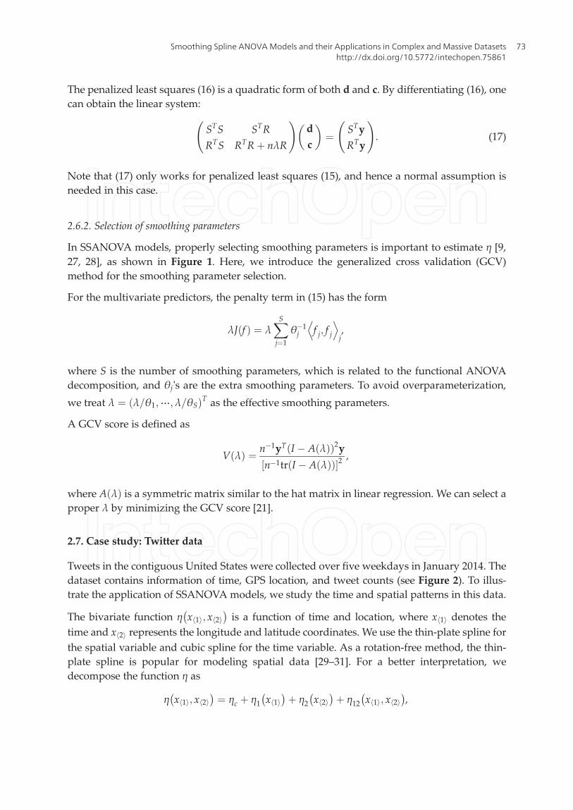
2.6.2. Selection of smoothing parameters

In SSANOVA models, properly selecting smoothing parameters is important to estimate η [9,

27, 28], as shown in Figure 1. Here, we introduce the generalized cross validation (GCV)

method for the smoothing parameter selection.

For the multivariate predictors, the penalty term in (15) has the form

λJ fð Þ ¼ λX

S

j¼1

θ�1j f j; f j

D E

j,

where S is the number of smoothing parameters, which is related to the functional ANOVA

decomposition, and θj's are the extra smoothing parameters. To avoid overparameterization,

we treat λ ¼ λ=θ1;⋯;λ=θSð ÞT as the effective smoothing parameters.

A GCV score is defined as

V λð Þ ¼n�1yT I � A λð Þð Þ2y

n�1tr I � A λð Þð Þ½ �2,

where A λð Þ is a symmetric matrix similar to the hat matrix in linear regression. We can select a

proper λ by minimizing the GCV score [21].

2.7. Case study: Twitter data

Tweets in the contiguous United States were collected over five weekdays in January 2014. The

dataset contains information of time, GPS location, and tweet counts (see Figure 2). To illus-

trate the application of SSANOVA models, we study the time and spatial patterns in this data.

The bivariate function η x 1h i; x 2h i

� �

is a function of time and location, where x 1h i denotes the

time and x 2h i represents the longitude and latitude coordinates. We use the thin-plate spline for

the spatial variable and cubic spline for the time variable. As a rotation-free method, the thin-

plate spline is popular for modeling spatial data [29–31]. For a better interpretation, we

decompose the function η as

η x 1h i; x 2h i

� �

¼ ηc þ η1 x 1h i

� �

þ η2 x 2h i

� �

þ η12 x 1h i; x 2h i

� �

,


73

where ηc is a constant function; η1 and η2 are the main effects of time and location, respectively;

and η12 is the spatial-time interaction effect.

The main effects of time and location are shown in Figure 3. Obviously, in panel (a), the

number of tweets has the periodic effect, where it attains the maximum value at 8:00 p.m. and

the minimum value at 5:00 a.m. The main effect of time shows the variations of Twitter usages

in the United States. In addition, we can infer how the tweet counts vary across different

locations based on panel (b) in Figure 3. There tend to be more tweets in the east than those

in the west regions and more tweets in the coastal zone than those in the inland. We use the

scaled dot product

π ¼ bη12

� �Tby=∥by∥2

to quantify the percentage decomposition of the sum of squares of by [11], where

by ¼ by1;…;byn� �T

is the predicted values of log #Tweetsð Þ, and bη12 ¼ η12 x1ð Þ;…; η12 xnð Þ� �T

is

the estimated interaction effect term, where η12 xð Þ ¼ η12 x 1h i; x 2h i

� �. In our fitted model,

Figure 2. Heatmaps of tweet counts in the contiguous United States. (a) Tweet counts at 2:00 a.m. (b) Tweet counts at

6:00 p.m.

Figure 3. (a) The main effect function of time (hours). (b) The main effect function of location.


π ¼ 3� 10�16, which is so small that the interaction term is negligible. This indicates that there

is no significant difference for the Twitter usages across time in the contiguous United States.

3. Efficient approximation algorithm in massive datasets

In this section, we consider SSANOVA models under the big data settings. The computational

cost of solving (17) is of the order O n3� �

and thus gives rise to a challenge on the application of

SSANOVA models when the volume of data grows. To reduce the computational load, an

obvious way is to select a subset of basis functions randomly. However, it is hard to keep the

data features by uniform sampling. In the following section, we present an adaptive basis

selection method and show its advantages over uniform sampling [14]. Instead of selecting

basis functions, another approach to reduce the computational cost is shrinking the original

sample size by rounding algorithm [15].

3.1. Adaptive basis selection

A natural way to select the basis functions is through uniform sampling. Suppose that we

randomly select a subset �x ¼ �x1;…; �x�n

� �from x1;…; xnf g, where �n is the subsample size.

Thus, the kernel matrix would be R �xi; x� �

, i ¼ 1,…, �n. Then, one minimizes (17) in the effective

model space:

HE ¼ N ⊕ span R �xi; x� �

; i ¼ 1; 2;…; �n� �

:

The computational cost will be reduced significantly to O n�n2ð Þ if �n is much smaller than n.

Furthermore, it can be proven that the minimizer of (2), �η, by uniform sampling basis selection,

has the same asymptotic convergence rate as the full basis minimizer bη.

Although the uniform basis selection reduces the computational cost and the corresponding �η

achieves the optimal asymptotic convergence rate, it may fail to retain the data features

occasionally. For example, when the data are not evenly distributed, it is hard for uniform

sampling to capture the feature where there are only a few data points. In [14], an adaptive

basis selection method is proposed. The main idea is to sample more basis functions where the

response functions change largely and fewer basis functions on those flat regions. More details

of adaptive basis selection method are shown in the following procedure:

Step 1 Divide the range of responses yi� �n

i¼1into K disjoint intervals, S1,…, SK. Denote ∣Sk∣ as

the number of observations in Sk.

Step 2 For each Sk, draw a random sample of size nk from this collection. Let

x∗ kð Þ ¼ x∗ kð Þ1 ;…; x

∗ kð Þnk

� be the predictor values.

Step 3 Combine x∗ 1ð Þ,…, x∗ Kð Þ together to form a set of sampled predictor values x∗1;…; x∗n∗� �

,

where n∗ ¼PK

k¼1 nk.


75

Step 4 Define

HE ¼ H0 ⊕ span R x∗i ; ��

; i ¼ 1; 2;…; n∗� �

as the effective model space.

By adaptive basis selection, the minimizer of (2) keeps the same form as that in Theorem 2.3:

ηA xð Þ ¼X

M

k¼1

dkξk xð Þ þX

n∗

i¼1

ciR x∗i ; x� �

:

Let R∗ be an n� n∗ matrix, and its i; jð Þth entry is R xi; x∗j

�

. Let R∗∗ be an n∗ � n∗ matrix, and its

i; jð Þth entry is R x∗i ; x∗

j

�

. Then, the estimator ηAsatisfies

ηA¼ SdA þ R∗cA,

where ηA¼ ηA x1ð Þ;⋯; ηA xn∗ð Þ� �T

, dA ¼ d1;…; dMð ÞT , and cA ¼ c1;…; cn∗ð ÞT . Similar to (17), the

linear system of equations in this case is

STS STR∗

RT∗S RT

∗R∗ þ nλR∗∗

!

dA

cA

�

¼STy

RT∗y

!

: (18)

The computational complexity of solving (18) is of the orderO nn∗2� �

, so the method decreases the

computational cost significantly. It can also be shown that the adaptive sampling basis selection

smoothing spline estimator ηA has the same convergence property as the full basis method. More

details about the consistency theory can be found in [14]. Moreover, adaptive sampling basis

selection method for exponential family smoothing spline models was developed in [32].

3.2. Rounding algorithm

Other than sampling a smaller set of basis functions to save the computational resources, for

example, the adaptive basis selection method presented previously, [15] proposed a new

rounding algorithm to fit SSANOVA models in the context of big data.

Rounding algorithm: The details of rounding algorithm can be shown in the following procedure:

Step 1 Assume that all predictors are continuous.

Step 2 Convert all predictors to the interval 0; 1½ �.

Step 3 Round the raw data by using the transformation:

zi jh i ¼ RD xi jh i=r jh i

� �

r jh i, for i∈ 1;⋯; nf g, j∈ 1;⋯; df g,

where the rounding parameter r jh i ∈ 0; 1ð � and rounding function RD �ð Þ transform input data to

the nearest integer.


Step 4 After replacing xi jh i with zi jh i, we redefine S and R in (16) and then estimate η by

minimizing the penalized least squares (16).

Remark 1 In Step 3, if r jh i is the rounding parameter for jth predictor and its value is 0.03, then

each zi jh i is formed by rounding the corresponding xi jh i to its nearest 0.03.

Remark 2 It is evident that the value of rounding parameter can influence the precision of

approximation. The smaller the rounding parameter, the better the model estimation and the

higher the computational cost.

Computational benefits: We now briefly explain why the implementation of rounding algo-

rithm can reduce the computational loads. For example, if the rounding parameter r ¼ 0:01, it

is obvious that u ≤ 101, where u denotes the number of uniquely observed values. In conclu-

sion, using user-tunable rounding algorithm can dramatically reduce the computational bur-

den of fitting SSANOVA models from the order of O n3� �

to O u3� �

, where u≪ n.

Case study: To illustrate the benefit of the rounding algorithm, we apply the algorithm to the

electroencephalography (EEG) dataset. Note that EEG is a monitoring method to record the

electrical activity of the brain. It can be used to diagnose sleep disorders, epilepsy, encephalop-

athies, and brain death.

The dataset [33] contains 44 controls and 76 alcoholics. Each subject was repeatedly measured

10 times by using visual stimulus at a frequency of 256 Hz. This brings about n ¼ 10 replica-

tions �120 subjects �256 time points ¼ 307; 200 observations. There are two predictors, time

and group (control vs. alcoholic). We apply the cubic spline to the time effect and the nominal

spline to the group effect.

After applying the model to the unrounded data, rounded data with rounding parameter

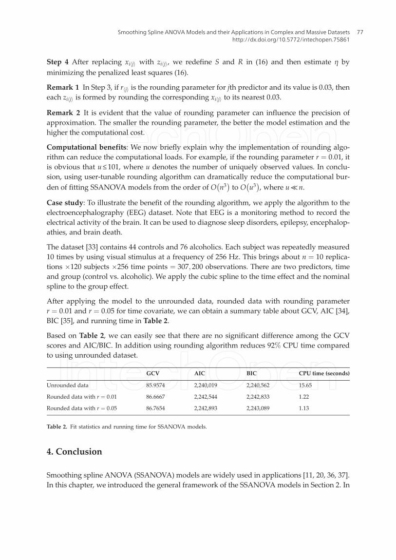
r ¼ 0:01 and r ¼ 0:05 for time covariate, we can obtain a summary table about GCV, AIC [34],

BIC [35], and running time in Table 2.

Based on Table 2, we can easily see that there are no significant difference among the GCV

scores and AIC/BIC. In addition using rounding algorithm reduces 92% CPU time compared

to using unrounded dataset.

4. Conclusion

Smoothing spline ANOVA (SSANOVA) models are widely used in applications [11, 20, 36, 37].

In this chapter, we introduced the general framework of the SSANOVA models in Section 2. In

GCV AIC BIC CPU time (seconds)

Unrounded data 85.9574 2,240,019 2,240,562 15.65

Rounded data with r ¼ 0:01 86.6667 2,242,544 2,242,833 1.22

Rounded data with r ¼ 0:05 86.7654 2,242,893 2,243,089 1.13

Table 2. Fit statistics and running time for SSANOVA models.


77

Section 3, we discussed the models under the big data settings. When the volume of data

grows, fitting the models is computing-intensive [11]. The adaptive basis selection algorithm

[14] and rounding algorithm [15] we presented can significantly reduce the computational cost.

Acknowledgements

This work is partially supported by the NIH grants R01 GM122080 and R01 GM113242; NSF

grants DMS-1222718, DMS-1438957, and DMS-1228288; and NSFC grant 71331005.

Conflict of interest

The authors whose names are listed immediately below certify that they have NO affiliations

with or involvement in any organization or entity with any financial interest (such as hono-

raria; educational grants; participation in speakers’ bureaus; membership, employment, con-

sultancies, stock ownership, or other equity interests; and expert testimony or patent-licensing

arrangements) or nonfinancial interest (such as personal or professional relationships, affilia-

tions, knowledge, or beliefs) in the subject matter or materials discussed in this manuscript.

Appendix

In this appendix, we use two examples to illustrate how to implement smoothing spline

ANOVA (SSANOVA) models in R. The gss package in R, which can be downloaded on the

CRAN https://cran.r-project.org/, is utilized.

We now load the gss package:

library(gss)

Example I: Apply the smoothing spline to a simulated dataset.

Suppose that the predictor x follows a uniform distribution on 0; 1½ �, and the response y is

generated based on y ¼ 5þ 2 cos 3πxð Þ þ e, where e � N 0; 1ð Þ.

x<-runif(100);y<-5+2*cos(3*pi*x)+rnorm(x)

Then, fit cubic smoothing spline model:

cubic.fit<-ssanova(y˜x)

To evaluate the predicted values, one uses:

new<-data.frame(x=seq(min(x),max(x),len=50))

est<-predict(cubic.fit,new,se=TRUE)


The se.fit parameter indicates if one can get the pointwise standard errors for the predicted

values. The predicted values and Bayesian confidence interval, shown in Figure 4, are gener-

ated by:

plot(x,y,col=1)

lines(new$x,est$fit,col=2)

lines(new$x,est$fit+1.96*est$se,col=3)

lines(new$x,est$fit-1.96*est$se,col=3)

Example II: Apply the SSANOVA model to a real dataset.

In this example, we illustrate how to implement the SSANOVA model using the gss package.

The data is from an experiment in which a single-cylinder engine is run with ethanol to see

how the nox concentration nox in the exhaust depends on the compression ratio comp and the

equivalence ratio equi. The fitted model contains two predictors (comp and equi) and one

interaction term.

data(nox)

nox.fit <- ssanova(log10(nox)˜comp*equi,data=nox)

The predicted values are shown in Figure 5.

x=seq(min(nox$comp),max(nox$comp),len=50)

y=seq(min(nox$equi),max(nox$equi),len=50)

temp <- function(x, y){

Figure 4. The solid red line represents the fitted values. The green lines represent the 95% Bayesian confidence interval.

The raw data are shown as the circles.


79

new=data.frame(comp=x,equi=y)

return(predict(nox.fit,new,se=FALSE))

}

z=outer(x, y, temp)

persp(x,y,z,theta = 30).

Author details

Jingyi Zhang, Honghe Jin, Ye Wang, Xiaoxiao Sun, Ping Ma* and Wenxuan Zhong

*Address all correspondence to: [email protected]

Department of Statistics, The University of Georgia, Athens, GA, USA

References

[1] Buja A, Hastie T, Tibshirani R. Linear smoothers and additive models. The Annals of

Statistics. 1989;17:453-510

[2] Burman P. Estimation of generalized additive models. Journal of Multivariate Analysis.

1990;32(2):230-255

Figure 5. The x-axis, y-axis, and z-axis represent the compression ratio, the equivalence ratio, and the predicted values,

respectively.


[3] Friedman JH, Grosse E, Stuetzle W. Multidimensional additive spline approximation.

SIAM Journal on Scientific and Statistical Computing. 1983;4(2):291-301

[4] Hastie TJ. Generalized additive models. In: Statistical Models in S. Routledge; 2017. pp.

249-307

[5] Stone CJ. Additive regression and other nonparametric models. The Annals of Statistics.

1985;13:689-705

[6] Stone CJ. The dimensionality reduction principle for generalized additive models. The

Annals of Statistics. 1986;14:590-606

[7] Barry D et al. Nonparametric bayesian regression. The Annals of Statistics. 1986;14(3):934-

953

[8] Chen Z. Interaction Spline Models. University of Wisconsin–Madison; 1989

[9] Gu C,Wahba G.Minimizing GCV/GML scores with multiple smoothing parameters via the

Newton method. SIAM Journal on Scientific and Statistical Computing. 1991;12(2):383-398

[10] Wahba G. Partial and Interaction Splines for the Semiparametric Estimation of Functions

of Several Variables. University of Wisconsin, Department of Statistics; 1986

[11] Gu C, Smoothing Spline ANOVA. Models, Volume 297. In: Springer Science & Business

Media; 2013

[12] Wahba G. Spline Models for Observational Data. SIAM; 1990

[13] Wang Y. Smoothing Splines: Methods and Applications. CRC Press; 2011

[14] Ma P, Huang JZ, Zhang N. Efficient computation of smoothing splines via adaptive basis

sampling. Biometrika. 2015;102(3):631-645

[15] Helwig NE, Ma P. Smoothing spline ANOVA for super-large samples: Scalable computa-

tion via rounding parameters. Statistics and Its Interface, Special Issue on Statistical and

Computational Theory and Methodology for Big Data. 2016;9:433-444

[16] Green PJ, Silverman BW. Nonparametric Regression and Generalized Linear Models: A

Roughness Penalty Approach. CRC Press; 1993

[17] Kimeldorf GS, Wahba G. A correspondence between Bayesian estimation on stochastic

processes and smoothing by splines. The Annals of Mathematical Statistics. 1970;41(2):

495-502

[18] Kimeldorf GS, Wahba G. Spline functions and stochastic processes. Sankhya: The Indian

Journal of Statistics, Series A; 1970. pp. 173-180

[19] O’sullivan F, Yandell BS, Raynor WJ Jr. Automatic smoothing of regression functions in

generalized linear models. Journal of the American Statistical Association. 1986;81(393):96-103

[20] Wahba G, Wang Y, Gu C, Klein R, Klein B. Smoothing spline ANOVA for exponential

families, with application to the Wisconsin epidemiological study of diabetic retinopathy.

The Annals of Statistics; 1995:1865-1895


81

[21] Craven P,Wahba G. Smoothing noisy data with spline functions. NumerischeMathematik.

1978;31(4):377-403

[22] Golub GH, Heath M, Wahba G. Generalized cross-validation as a method for choosing a

good ridge parameter. Technometrics. 1979;21(2):215-223

[23] Kreyszig E. Introductory Functional Analysis with Applications, Volume 1. New York:

Wiley; 1989

[24] Berlinet A, Thomas-Agnan C. Reproducing Kernel Hilbert Spaces in Probability and

Statistics. In: Springer Science & Business Media; 2011

[25] Aronszajn N. Theory of reproducing kernels. Transactions of the American Mathematical

Society. 1950;68(3):337-404

[26] Abramowitz M, Stegun IA. Handbook of Mathematical Functions: With Formulas,

Graphs, and Mathematical Tables, Volume 55. Courier Corporation; 1964

[27] Hurvich CM, Simonoff JS, Tsai C-L. Smoothing parameter selection in nonparametric

regression using an improvedAkaike information criterion. Journal of the Royal Statistical

Society: Series B (Statistical Methodology). 1998;60(2):271-293

[28] Mallows CL. Some comments on Cp. Technometrics. 2000;42(1):87-94

[29] Duchon J. Splines minimizing rotation-invariant semi-norms in Sobolev spaces. Construc-

tive Theory of Functions of Several Variables; 1977. pp. 85-100

[30] Meinguet J. Multivariate interpolation at arbitrary points made simple. Zeitschrift für

Angewandte Mathematik und Physik (ZAMP). 1979;30(2):292-304

[31] Wahba G,Wendelberger J. Some newmathematical methods for variational objective anal-

ysis using splines and cross validation. Monthly Weather Review. 1980;108(8):1122-1143

[32] Ma P, Zhang N, Huang JZ, Zhong W. Adaptive basis selection for exponential family

smoothing splines with application in joint modeling of multiple sequencing samples.

Statistica Sinica, in press; 2017

[33] Lichman M. UCI Machine Learning Repository. 2013. URL. http://archive.ics.uci.edu/ml

[34] Akaike H. Information theory and an extension of the maximum likelihood principle. In:

Parzen E, Tanabe K, Kitagawa G, editors. Selected Papers of Hirotugu Akaike, Springer

Series in Statistics. New York: Springer; 1998. pp. 199-213

[35] Schwarz G. Estimating the dimension of a model. The Annals of Statistics. 1978;6(2):461-

464. DOI: 10.1214/aos/1176344136

[36] Helwig NE, Shorter KA, Ma P, Hsiao-Wecksler ET. Smoothing spline analysis of variance

models: A new tool for the analysis of cyclic biomechanical data. Journal of Biomechanics.

2016;49(14):3216-3222

[37] Lin X, Wahba G, Xiang D, Gao F, Klein R, Klein B. Smoothing spline ANOVA models for

large data sets with Bernoulli observations and the randomized GACV. The Annals of

Statistics. 2000;28:1570-1600


smoothing spline anova models and their applications in

Documents