smoke simulation on programmable graphics hardware...

SMOKE SIMULATION ON PROGRAMMABLE GRAPHICS HARDWARE

A THESIS SUBMITTED TO THE GRADUATE SCHOOL OF NATURAL AND APPLIED SCIENCES

OF MIDDLE EAST TECHNICAL UNIVERSITY

BY

GÖKÇE YILDIRIM

IN PARTIAL FULFILLMENT OF THE REQUIREMENTS FOR

THE DEGREE OF MASTER OF SCIENCE IN

COMPUTER ENGINEERING

SEPTEMBER 2005

Approval of the Graduate School of Natural and Applied Sciences

Prof. Dr. Canan Özgen Director

I certify that this thesis satisfies all the requirements as a thesis for the degree of Master of Science.

Prof. Dr. Ayşe Kiper Head of Department

This is to certify that we have read this thesis and that in our opinion it is fully adequate, in scope and quality, as a thesis for the degree of Master of Science. Assoc. Prof. Dr. Veysi İşler Supervisor Examining Committee Members Prof. Dr. Ayşe Kiper (METU, CENG) Assoc. Prof. Dr. Veysi İşler (METU, CENG) Prof. Dr. Volkan Atalay (METU, CENG) Asst. Prof. Dr. Harun Artuner (Hacettepe Univ., CENG) Asst. Prof. Dr. Halit Oğuztüzün (METU, CENG)

iii

I hereby declare that all information in this document has been obtained and presented in accordance with academic rules and ethical conduct. I also declare that, as required by these rules and conduct, I have fully cited and referenced all material and results that are not original to this work. Name, Last name : Signature :

iv

ABSTRACT

SMOKE SIMULATION ON PROGRAMMABLE GRAPHICS HARDWARE

Yıldırım, Gökçe

MSc., Department of Computer Engineering

Supervisor: Assoc. Prof. Dr. Veysi İşler

September 2005, 72 pages

Fluids such as smoke, water and fire are simulated for both Computer

Graphics applications and engineering fields such as Mechanical Engineering.

Generally, Fluid Dynamics is used for the achievement of realistic-looking fluid

simulations. However, the complexity of these calculations makes it difficult to

achieve high performance. With the advances in graphics hardware, it has been

possible to provide programmability both at the vertex and the fragment level,

which allows for faster simulations of complex fluids and other events.

In this thesis, one gaseous fluid, smoke is simulated in three dimensions by

solving Navier-Stokes Equations (NSEs) using a semi-Lagrangian unconditionally

stable method. Simulation is performed both on Central Processing Unit (CPU) and

Graphics Processing Unit (GPU). For the programmability at the vertex and the

fragment level, C for Graphics (Cg), a platform-independent and architecture neutral

v

shading language, is used. Owing to the advantage of programmability and

parallelism of GPU, smoke simulation on graphics hardware runs significantly faster

than the corresponding CPU implementation. The test results prove the higher

performance of GPU over CPU for running three dimensional fluid simulations.

Keywords: Graphics hardware, GPU, Navier-Stokes equations (NSEs), Smoke

simulation

vi

ÖZ

PROGRAMLANABİLİR GRAFİK İŞLEMCİDE DUMAN SİMÜLASYONU

Yıldırım, Gökçe

Yüksek Lisans, Bilgisayar Mühendisliği Bölümü

Tez Yöneticisi: Doç. Dr. Veysi İşler

Eylül 2005, 72 sayfa

Duman, su ve ateş gibi akışkanlar hem Bilgisayar Grafiği uygulamalarında

hem de Makine Mühendisliği gibi mühendislik alanlarında yaygın olarak simüle

edilmektedir. Genel olarak, gerçekçi görünüşlü akışkan simülasyonu elde etmek

için akışkan dinamiği kullanılmaktadır. Ancak, bu hesaplamaların karmaşıklığı

yüksek performans elde etmeyi zorlaştırmaktadır. Grafik donanımındaki gelişmeler

sayesinde, köşe ve parça seviyesinde programlama yapabilmek mümkün olmuştur.

Bu sayede, karmaşık akışkanların ve diğer olayların daha hızlı simülasyonları

mümkün olabilmektedir.

Bu tezde, gaz halindeki bir akışkan olan duman, yarı Lagrangian koşulsuz

kararlı bir yöntem ile Navier-Stokes denklemleri çözülerek üç boyutlu olarak simüle

edilmektedir. Bu simülasyon ana işlemcide ve grafik işlemcide gerçeklenmektedir.

Köşe ve parça seviyesinde programlama yapmak için platform bağımsız ve mimari

vii

tarafsız bir gölgelendirme dili olan Grafik için C kullanılmaktadır. Grafik işlemcinin

programlanabilme ve paralellik özellikleri sayesinde, bu duman simülasyonu grafik

donanımı üzerinde ana işlemcidekine göre büyük ölçüde hızlı çalışmaktadır. Test

sonuçları, üç boyutlu akışkan simülasyonları için, grafik işlemcinin ana işlemciye

gore yüksek performansla çalıştığını ispatlamaktadır.

Anahtar Kelimeler: Grafik işlemci programlama, GPU, Navier-Stokes denklemleri

(NSEs), duman simülasyonu

viii

To My Family

ix

ACKNOWLEDGMENTS

I wish to express my deepest gratitude to my supervisor Assoc. Prof. Dr. Veysi İşler

for his guidance, advice, criticism, encouragements and insight throughout the

research.

I would also like to thank my friends for their suggestions and valuable comments

during this study. Moreover, I would like to express my deep appreciation to my

family for their support during the thesis.

x

TABLE OF CONTENTS

ABSTRACT............................................................................................................... iv

ÖZ .............................................................................................................................. vi

ACKNOWLEDGMENTS ......................................................................................... ix

TABLE OF CONTENTS............................................................................................ x

LIST OF TABLES....................................................................................................xii

LIST OF FIGURES .................................................................................................xiii

CHAPTER 1 ............................................................................................................... 1

INTRODUCTION .................................................................................................. 1

CHAPTER 2 ............................................................................................................... 5

RECENT WORK.................................................................................................... 5

2.1 Literature Survey .......................................................................................... 5

2.2 Graphics Hardware ....................................................................................... 8

2.2.1 History of Graphics Hardware............................................................... 9

2.2.2 Graphics Hardware Pipeline ................................................................ 10

2.2.3 High-Level Shading Languages........................................................... 17

2.3 Fluid Simulations on GPU.......................................................................... 18

CHAPTER 3 ............................................................................................................. 20

IMPLEMENTATION........................................................................................... 20

3.1 Fluid Flow Equations.................................................................................. 20

3.2 Solving Fluid Flow Equations .................................................................... 28

3.2 CPU Implementation .................................................................................. 36

3.2.1 Evolution of Velocity........................................................................... 38

xi

3.2.2 Evolution of Temperature and Density................................................ 43

3.3 GPU Implementation .................................................................................. 45

3.3.1 Differences between CPU and GPU Implementations ........................ 46

3.3.2 Implementation Details........................................................................ 50

3.4 Rendering.................................................................................................... 59

CHAPTER 4 ............................................................................................................. 62

DISCUSSION AND RESULTS........................................................................... 62

CHAPTER 5 ............................................................................................................. 66

CONCLUSION AND FUTURE WORKS ........................................................... 66

5.1 Future Works .............................................................................................. 67

REFERENCES ......................................................................................................... 68

xii

LIST OF TABLES

Table 3.1 Vector Calculus Operators Used in Fluid Flow Equations ...................... 23

Table 4.1 Comparison of Performance on CPU and GPU....................................... 65

xiii

LIST OF FIGURES

Figure 2.1: Graphics Hardware Pipeline.................................................................. 11

Figure 2.2: Programmable Graphics Pipeline.......................................................... 13

Figure 2.3: Programmable Vertex Processor Flow Chart........................................ 14

Figure 2.4: Programmable Fragment Processor Flow Chart. .................................. 16

Figure 3.1: A Single Grid Cell................................................................................. 21

Figure 3.2: Advection Step. ..................................................................................... 32

Figure 3.3: Discretized Three Dimensional grid. .................................................... 37

Figure 3.4: Pseudo Code of the General Loop in CPU Implementation. ................ 38

Figure 3.5: Steps in Evolution of Velocity. ............................................................. 39

Figure 3.6: Pseudo Code of Velocity Update Step. ................................................. 39

Figure 3.7: Pseudo Code of the Step of Addition of Forces. ................................... 40

Figure 3.8: Pseudo Code of Diffusion Step. ............................................................ 41

Figure 3.9: Pseudo Code of Projection Step. ........................................................... 42

Figure 3.10: Pseudo Code of Advection Step.......................................................... 43

Figure 3.11: Steps in Evolution of Scalar Values.................................................... 44

Figure 3.12: Pseudo Code of Density Update Step. ................................................ 44

Figure 3.13: Pseudo Code of the Step of Addition of Sources. ............................... 45

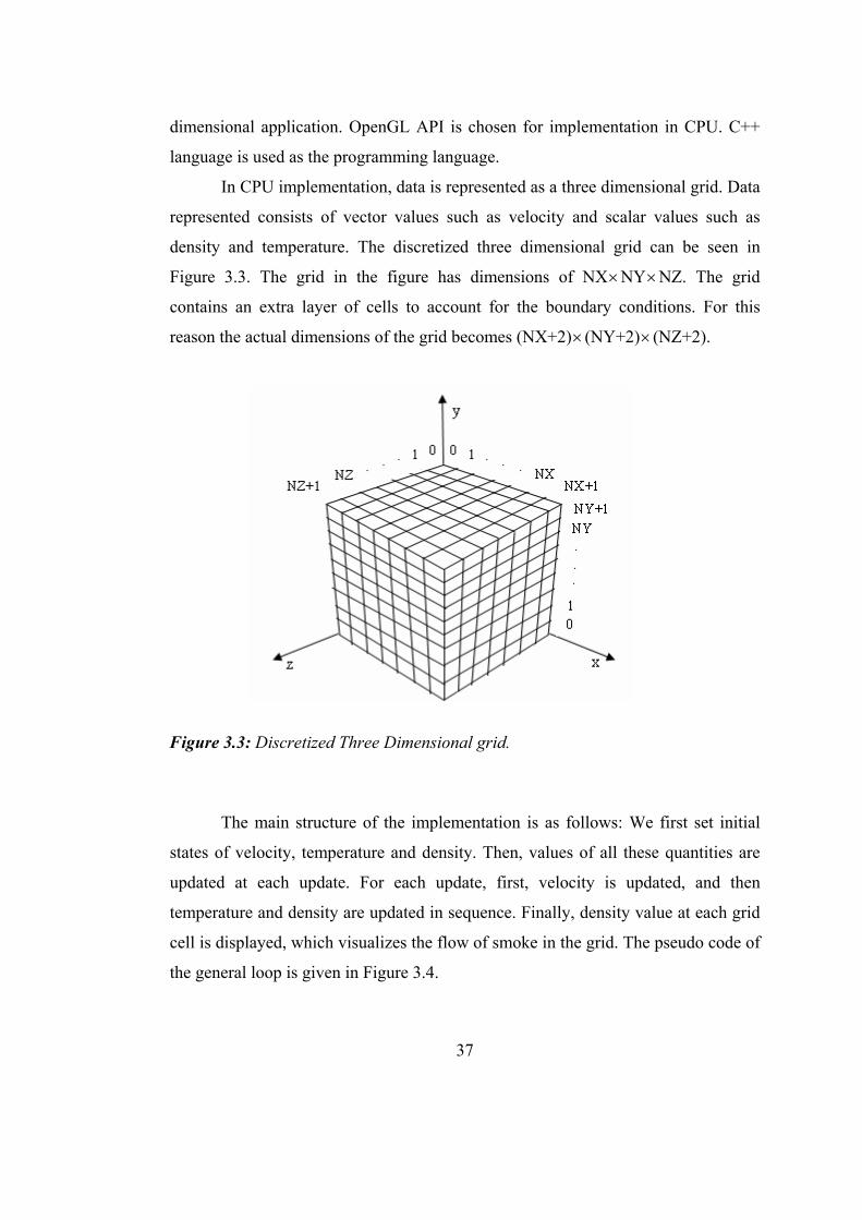
Figure 3.14: Comparison of 3D Textures and Flat 3D Textures. ............................ 47

Figure 3.15: Algorithm Flow for Velocity Texture on GPU. .................................. 48

Figure 3.16: Algorithm Flow for Texture of Scalar Values on GPU. ..................... 49

Figure 3.17: Copy-to-Texture Mechanism. ............................................................. 49

Figure 3.18: Render-to-Texture Mechanism. .......................................................... 50

Figure 3.19: Pseudo Code of the Main Loop on GPU Implementation. ................. 51

xiv

Figure 3.20: Pseudo Code of Cg Setup.................................................................... 53

Figure 3.21: Cg Code of Vertex Shader Program.................................................... 54

Figure 3.22: Pseudo Code of Performing Computations on Textures..................... 55

Figure 3.23: Pseudo Code of Processing of Fragment Programs. ........................... 56

Figure 3.24: addForce Cg Fragment Program Code. ............................................... 58

Figure 3.25: 2D Axis-aligned Texture Slices. ......................................................... 60

Figure 3.26: Arrangement of Texture Slices According to View Direction............ 61

Figure 3.27 Smoke Images Rendered with Different Methods. .............................. 61

Figure 4.1: Flat 3D Texture of Flowing Smoke in a Grid of 16×32×16 Voxels.... 62

Figure 4.2: Flowing of Smoke in a Grid of 16×32×16 Voxels in Upward Direction

in Movement Sequence of (a), (b), (c) and (d). ........................................................ 64

1

CHAPTER 1

INTRODUCTION

The main goal of computer graphics is to simulate nature in a realistic

manner. The broadness of natural phenomena presents difficult challenges in

computer graphics. One kind of natural phenomena, fluids, exist in everyday life

and form a basis for a wide range of natural phenomena. Real-time simulation of

fluids such as water, smoke, clouds and fire is widely used in movies, games and

simulators. Moreover, modeling and simulation of fluids has great importance in

many engineering fields such as mechanical engineering. Thus, fluid simulation is a

popular and challenging research topic. This challenge is an expected result due to

high complexity of fluid dynamics. Properties and behaviors of fluid have been

studied for many years in Computational Fluid Dynamics (CFD). However, the goal

of researches in CFD is to obtain a highly accurate fluid behavior, while the main

goal in computer graphics is to achieve physically based realistic-looking results

with high performance. Despite the precedence of accuracy in CFD, efficiency is

mostly prior in computer graphics applications. This thesis also aims to achieve high

performance in physical computations as well as having physically based realistic-

looking smoke.

There are two main approaches used in fluid simulation: Lagrangian particle-

based and Eulerian grid-based approaches. Many different methods have been

developed on both approaches. In particle-based methods, fluid is composed of

particles which dynamically change over time as a result of external forces.

Lagrangian methods start from the motion of fluid particles to analyze their

trajectory as a function of time. Each particle has different attributes such as

2

position, mass and velocity. Basically, particles are moved by applying forces,

calculating acceleration and velocity, and updating position. Simplicity of particles

makes these methods advantageous [1]. Moreover, particle-based methods guarantee

mass conversation. On the other hand, an important drawback of particle-based

simulations is the difficulty of representing smooth surfaces of fluids using particles

[2]. A detailed surface requires a high density of particles near surfaces.

The second kind of approaches used in fluid simulations are Eulerian grid-

based methods. In recent years grid-based methods have been used very often in

fluid simulations. In these methods, the spatial domain is discretized into small cells

to form a volume grid. Eulerian methods start from the spatial fixed points to

analyze the properties of the fluid at these points as a function of time [4]. Eulerian

equations are discretized to calculate different attributes of each grid cell such as

pressure, density, force and velocity.

Incompressible Navier-Stokes equations (NSEs), which are extensions to

Eulerian equations including the effects of viscosity on the flow, describe fluid flow

fully using momentum and mass conservation [3]. Navier-Stokes equations consist

of a set of partial differential equations that describe the flow of fluids. Different

methods to solve Navier-Stokes equations have been developed and used in

physically based fluid simulations. In this thesis, a semi-Lagrangian method, which

is unconditionally stable, is used to solve Navier-Stokes equations in simulation of

one gaseous phenomena, smoke [5].

Physically based fluid simulations are common in engineering fields as well

as computer graphics. However, realistic-looking physically based fluid simulations

are computationally expensive since they require solutions of many complex

equations. Thus, achievement of fast fluid simulations is a big problem.

In recent years, with the development of fast hardware, there has been a shift

from fixed-pipeline to programmable pipeline in graphics hardware. In this way,

Graphics Processing Unit (GPU) has been able to provide programmability both at

the fragment level and the vertex level. Especially, after the support of IEEE 32 bits

float precision in the fragment program, GPU has been more popular to solve

3

general-purpose problems in real-time [6]. The parallel nature of fluid flow

computations makes GPU programming useful for fluid simulations. Thus, with the

advantage of parallelism and programmability of GPU, there has been a lot of

studies to move fluid flow computations from Central Processing Unit (CPU) to

GPU. These works are very recent and mainly focus on two dimensional domain for

its simplicity [41, 45, 46, 49]. Boundary conditions are processed simply on two

dimensional domain because of the lack of flexible control operations on GPU.

In this thesis, three dimensional simulation of smoke is performed on both

CPU and GPU. Data in this simulation is represented on a three dimensional grid of

cells. For the physical simulation of smoke behavior, Navier-Stokes equations are

solved using a semi-Lagrangian unconditionally stable method. Both CPU and GPU

implementations use the same method basically. Thus, for comparison, the results

reliably show the difference in speed of computations. Owing to the parallelism in

graphics hardware, smoke simulation performed on GPU runs significantly faster

than the corresponding CPU implementation. In CPU implementation, grid cells are

represented in an array, while in GPU implementation, data is stored in textures, i.e.

the analogy of arrays on GPU. For the representation of three dimensional data, flat

3D textures, in which slices of volume are arranged in two dimensions, are used.

The use of flat 3D textures reduces the number of rendering passes, since the whole

three dimensional data is processed in one render. Three dimensional data consists

of different scalar attributes such as density, and vector attributes such as velocity.

Appropriate scalar attributes are packed into a single RGBA texel at fragment level.

In this way, the number of rendering passes is decreased by reducing the number of

textures to be processed. Furthermore, to improve the performance of GPU

implementation, double-buffered offscreen floating point rendering targets are

utilized, which decreases context switches.

Vertex and fragment programs are written in C For Graphics (Cg) in this

thesis. Fragment programs process each fragment data stored in flat 3D textures in

parallel. This is the main reason of the significant performance of GPU over CPU

which works by iterating over each grid cell.

4

In addition to implementing a three dimensional smoke simulation on both

CPU and GPU, one of the goals of this thesis is to accumulate experiences of GPU

programming of general-purpose computations and strategies of optimizations. This

is important since this experience will evolve into an optimization system for

various general-purpose computation problems, other than fluids.

The outline of this thesis is as follows: In Chapter 2, the literature about fluid

simulation in computer graphics is surveyed. Next, as well as basic concepts,

evolution of graphics hardware and some recent fluid simulations on GPU are

described. Then in Chapter 3, the equations of fluid dynamics used in this smoke

simulation as well as details of CPU and GPU implementations are explained. In the

next chapter, CPU and GPU results are compared and discussed. Finally, in Chapter

5, the thesis is concluded with a list of future works.

5

CHAPTER 2

RECENT WORK

This chapter presents recent work on development of physically based fluid

simulation. In the first section, a literature survey about fluid simulation is given.

The second section explains the development of graphics hardware and gives

detailed information about GPU. It is followed by a section which mentions some

fluid simulation applications developed on GPU recently.

2.1 Literature Survey

The physically based simulation of fluids such as smoke has received much

attention in computer graphics field for many years. There has been a lot of studies

in fluid simulation [3, 5, 10, 14, 20]. In this section, a survey about the recent studies

is done. Since this thesis is based on the Eulerian grid-based approach, this survey

refers mostly to such methods.

Particle systems were introduced into computer graphics by Reeves as a

method of modeling some natural phenomena such as fire, smoke and grass [1].

Instead of modeling these phenomena with polygons that define a boundary, Reeves

suggested modeling them with primitive particles that fill their volume. Miller and

Pearce used this idea to animate viscous fluids by simulating the forces of particles

interacting with each other [7]. O'Brien and Hodgins described the dynamic

behaviors of splashing fluids using particles [8].

An alternative method, Smoothed Particle Hydrodynamics (SPH) was

developed by Lucy [10] and by Gingold and Monaghan [11] for the simulation of

6

astrophysical problems. SPH is an interpolation method for particle systems. The

values of continuous variables are determined by an interpolation or smoothing of

the nearby particle distribution using smoothing kernels. Due to the gridless nature

of the method, resolution is controlled by the smoothing length which is a measure

of the mean inter-particle spacing. However, the method is general enough to be

used in any kind of fluid simulation. SPH was firstly introduced into computer

graphics to simulate fire and other gaseous phenomena by Stam and Fiume [9].

Desbrun and Gascuel extended SPH for simulating highly deformable substances

with particle systems [12]. In recent years, Müller et al. used an interactive method

based on SPH to simulate fluids with free surfaces [13]. They proposed methods to

track and visualize the free surface using point splatting and marching cubes-based

surface reconstruction. Furthermore, very recently, Müller et al. presented a method

to model and animate volumetric objects with material properties in the range from

stiff elastic to highly plastic [14]. In their method, both the volume and the surface

representation are point based, which allows large deformations.

Although it is a flexible method, one disadvantage of SPH is that it can only

solve flow of compressible fluids. Premože et al. used Moving Particle Semi-

Implicit (MPS), which is another gridless particle method [15]. This method solves

Navier-Stokes equations for incompressible fluids. Thus, it is advantageous to

simulate many kinds of fluid flow using MPS. However, since it is a Lagrangian

method, inflow and outflow of fluid is not allowed.

While Lagrangian methods are based on particles, Eulerian methods are grid-

based. Grid-based methods have been quite popular for fluid simulations in

computer graphics. In these methods, Navier-Stokes equations are discretized onto

the grid of cells. The properties in each cell are calculated according to these

equations. Two kinds of discretization are used mostly: Staggered grids and non-

staggered grids. The staggered grid representation stores velocity values at the grid

cell faces [16] and all scalar values at the grid cell centers while in non-staggered

grids all variables are defined at the center of cells [17].

7

In early days, Kass and Miller introduced a method for animating water

based on a simple, rapid and stable solution of a set of partial differential equations

resulting from an approximation to the shallow water equations [18]. They solved

the wave equation on the height field with an implicit method on a uniform finite-

difference grid. Chen and Lobo [19] computed the surface velocity height by

solving Navier-Stokes equations in two dimensions. They used the pressure field to

simulate the surface height of fluid. Usage of height field to simulate fluid surface

avoids expensive three dimensional computations [4]. However, this results in a less

realistic three dimensional fluid simulation. Furthermore, this technique does not

cover wave effects, mass transport and submerged obstacles.

To simulate the turbulence in smoke, Stam [20] decomposed the turbulent

wind field into two components: a deterministic component to specify large-scale

behaviour and a stochastic component to model turbulent small-scale behaviour.

Stam used Kolmogorov spectrum to model the small-scale random vector field in

this work. Foster and Metaxas [3] used an explicit integration scheme based on

Navier-Stokes equations which couple momentum and mass conservation to

completely describe complex fluid motion. They used Marker and Cells (MAC)

method to describe the free surface of fluid. One year later, Foster and Metaxas [21]

described a method that combines specialized forms of the equations of motion of a

hot gas with an efficient method for solving volumetric differential equations at low

resolutions. In works of Foster and Metaxas, to ensure stability for an animation, the

time step should be small. To diminish this instability problem, Stam [5] introduced

the semi-Lagrangian unconditionally stable method to solve Navier-Stokes

equations. However, the numerical dissipation was severe in this method. Fedkiw et

al. introduced a physically consistent vorticity confinement term to model the small

scale rolling features characteristic of smoke, which most coarse grid simulations

suffered from [22]. Being inspired by this model, Enright et al. [23] proposed a

particle level set method to model the complex surface of water. It is a hybrid

surface tracking method that uses massless marker particles combined with a

dynamic implicit surface. Foster and Fedkiw [24] combined the semi-Lagrangian

8

method with a novel adaptive technique for evolving an implicit surface to animate

viscous liquids ranging from water to thick mud. Furthermore, Fedkiw et al. [25]

used semi-Lagrangian method with vorticity confinement method to model both

vaporized fuel and hot gaseous products. Similarly, Rasmussen et al. [26] utilized

the semi-Lagrangian method to simulate the large-scale smoke in two dimensions

and combined two dimensional high resolution physically based flow fields with a

moderate sized three-dimensional Kolmogorov velocity field tiled periodically in

space. Very recently, Losasso et al. simulated smoke and water on an octree grid

addressing the memory requirements to some degree [27]. However, small scale

detail to be formed is very dependent on the refinement criteria. Furthermore,

Goktekin et al. [28] described a technique for animating the behavior of viscoelastic

fluids, which exhibit a combination of both fluid and solid characteristics. They

computed the elastic terms by integrating and advecting strain-rate throughout the

fluid.

After a literature survey on fluid simulation methods, it can be concluded

that both Eulerian methods and Lagrangians method have advantages and

disadvantages. While Lagrangian methods are easy to describe, keep mass

conservation and control, it is difficult to describe the smooth surfaces with particles

in Lagrangian methods. On the other hand, it is easier to describe complex surfaces

and analyze the fluid flow with the grid-based Eulerian methods. However, the need

to predefine the whole grid leads to cubic complexity. Thus, to overcome these

disadvantages, often some methods such as the popular semi-Lagrangian method

integrate Eulerian method with particles.

2.2 Graphics Hardware

Since physically based realistic-looking fluid simulations require complex

computations, achieving real-time performance has been a big problem in computer

graphics field. Computer graphics researchers have always struggled to develop

acceleration methods for fluid flow methods. Thus, with the development of the

9

programmable graphics hardware, many researchers turned to GPU to accelerate the

fluid flow computations. This thesis is also based on solutions of Navier-Stokes

equations to simulate smoke on GPU; for ths reason, it is worth to explain evolution

of graphics hardware. In this section, following the history of hardware, graphics

hardware pipeline and programmable graphics pipeline are explained. Moreover,

programmable vertex and fragment processors are mentioned briefly. Finally, high-

level shading languages are described.

2.2.1 History of Graphics Hardware

Recent developments in graphics hardware technology have allowed a

change in the implementation of the fixed pipeline used in graphics hardware.

Instead of a fixed set of functions, current processors allow a large amount of

programmability by letting the user develop special programs to be executed on

fragment and vertex level.

There are three main forces which have had effect on this rapid development

on graphics hardware. Firstly, doubling the number of transistors in semiconductor

industry provides a constant redoubling of computer power, which is known as

Moore’s Law. This means cheaper and faster computer hardware. The other

effective force is the requirement of a large amount of computations to simulate real

world. Third force which connects these two factors is the desire of human beings to

be simulated and entertained visually [29].

There have been four generations of GPU evolution so far [29]. With each

generation, better performance and evolving programmability has been delivered.

Before introduction of GPU, companies such as Silicon Graphics (SGI) and Evans

& Sutherland designed specialized and expensive graphics hardware. Although

these graphics systems were very important for the development of computer

graphics, they were too expensive to achieve mass-market success.

The first-generation GPUs were capable of rasterizing pre-transformed

triangles and applying one or two textures. Some examples of first-generation GPUs

10

which were produced until 1998 are NVIDIA’s TNT2 and ATI’s Rage. GPUs of this

generation suffer from transformation of vertices of three dimensional objects and

having a quite limited set of math operations for combining textures to compute the

color of rasterized pixels.

The second-generation GPUs include GPUs which were produced between

1999 and 2000 such as NVIDIA’s GeForce 256 and GeForce2, ATI’s Radeon 7500.

GPUs of this generation are able to do three dimensional vertex transformation and

lighting (T&L). Both OpenGL and DirectX 7 support hardware vertex

transformation. Although the set of math operations for combining textures and

coloring pixels are extended, possibilities are still limited.

The third-generation GPUs which were produced in 2001 include NVIDIA’s

GeForce3 and GeForce4 Ti and ATI’s Radeon 8500. This generation provides

vertex programmability. Considerably more pixel-level configurability is available

in this generation. Because of support to vertex programmability, but lacking of full

pixel programmability, this generation is accepted as transitional.

The fourth and the current generation of GPUs which have been produced

after 2002 until now includes NVIDIA’s GeForce FX family and ATI’s Radeon

9700. These GPUs provide both vertex-level and pixel-level programmability. They

are able to do complex vertex transformation and pixel-shading operations. DirectX

9 and various OpenGL extensions reveal the vertex-level and pixel-level

programmability of these GPUs.

2.2.2 Graphics Hardware Pipeline

A pipeline is a sequence of stages operating in parallel and in a fixed order.

Each stage in a pipeline takes input and from the previous stage and sends it as

output to the next stage. Figure 2.1 shows the graphics hardware pipeline used by

today’s GPUs. Three dimensional graphics application sends GPU a sequence of

vertices each of which has a position and several other attributes such as color,

texture coordinates and normal vector.

11

VertexTransformations

RasterOperations

Vertices TransformedVertices

PixelUpdates

FragmentsColored

Fragments

Pixel Positions

Vertex Connectivity

Figure 2.1: Graphics Hardware Pipeline (Inspired by [30]).

The first processing stage of the graphics hardware pipeline is vertex

transformation. A sequence of math operations is performed on each vertex in this

stage. These operations include transformation of the vertex position into a screen

position for use by the rasterizer, generation of texture coordinates for texturing and

lighting of the vertex for the determination of its color.

The second stage is primitive assembly and rasterization stage. The

transformed vertices from vertex transformation stage flow into this stage. First, the

primitive assembly step assembles vertices into geometric primitives. This results in

a sequence of triangles, lines or points. These primitives may require clipping to the

view frustum. The rasterizer may also discard polygons based on the direction

polygons face; either forward or backward, which is known as culling. After the

clipping and culling steps, remaining polygons get into the rasterization step.

Rasterization is the process of determining the set of pixels covered by a geometric

primitive. Polygons, lines and points are each rasterized according to the rules

specified for each type of primitive. The result of rasterization is a set of pixel

locations as well as a set of fragments.

The term pixel is short for “picture element”. A pixel represents the contents

of the frame buffer at a specific location, such as the color, depth, and any other

values associated with that location. On the other hand, a fragment is the state

required potentially to update a particular pixel. The term “fragment” is used

12

because rasterization breaks up each geometric primitive such as a triangle into

pixel-sized fragments for each pixel that the primitive covers. A fragment has an

associated pixel location, a depth value, and a set of interpolated parameters such as

a color, a secondary (specular) color and one or more texture coordinate sets. These

various interpolated parameters are derived from the transformed vertices that make

up the particular geometric primitive used to generate the fragments.

Once a primitive is rasterized into a collection of zero or more fragments, the

interpolation, texturing, and coloring stage interpolates the fragment parameters as

necessary. This stage also performs a sequence of texturing and math operations.

The coloring step determines a final color for each fragment. Furthermore, this stage

may also determine a new depth or may even discard the fragment to avoid updating

the frame buffer’s corresponding pixel. Thus, this stage emits one or zero colored

fragments for every input fragment it receives.

The final stage of the hardware pipeline is the raster operations stage. This

stage performs a final sequence of per-fragment operations immediately before

updating the frame buffer. Raster operations stage checks each fragment based on

many tests such as alpha, stencil, and depth tests. These tests involve the fragment’s

final color or depth, the pixel location and per-pixel values such as the depth value

and stencil value of the pixel. If any test fails, this stage discards the fragment

without updating the pixel’s color value. After the tests, a blending operation

combines the final color of the fragment with the corresponding pixel’s color value.

Finally, a frame buffer write operation replaces the pixel’s color with the blended

color.

After brief information about fixed graphics hardware pipeline, the

programmable graphics pipeline can be seen in Figure 2.2. This figure shows vertex

and fragment stages of a programmable GPU.

13

Figure 2.2: Programmable Graphics Pipeline (Inspired by [30]).

The programmable vertex processor is the hardware unit that runs vertex

shader programs, while the programmable fragment processor is the unit that runs

fragment shader programs.

Figure 2.3 shows a flow chart of a programmable vertex processor. The flow

chart starts with loading each vertex’s attributes such as position, color and texture

coordinates into the vertex processor. The vertex processor then repeatedly fetches

the next instruction and executes it until the vertex program terminates. Instructions

access distinct sets of registers that contain vector values such as position, normal or

color. The vertex attribute registers are read-only and contain the set of attributes

specified by the application for the vertex. The temporary registers can be read and

written. As it can be understood from their names, they are used for computing

intermediate results. The output result registers are write-only. The vertex program

is responsible for writing its results to these registers. When the program terminates,

the output result registers contain the newly transformed vertex.

14

BeginVertex

Copy VertexAttributes to

Input Registers

VertexProgram

InstructionMemory

Emit OutputRegisters AsTransformed

Vertex

Fetch & DecodeNext Instruction

No

Yes

Perform InstructionMath/Operation

Map Input Values:Swizzle, Negate, etc.

Read Input and/orTemporary Registers

InputRegisters

TemporaryRegisters

OutputRegisters

VertexProgram

InstructionLoop

Figure 2.3: Programmable Vertex Processor Flow Chart (Inspired by [30]).

15

After triangle setup and rasterization stages, the interpolated values for each

register are passed to the fragment processor.

Figure 2.4 shows the flow chart of a programmable fragment processor. As

in the case of programmable vertex processor, the data flow involves executing a

sequence of instructions until the program terminates. There is a set of input

registers as in programmable vertex processor. However, rather than vertex

attributes, these read-only input registers contain interpolated per-fragment

parameters derived from the per-vertex parameters of the fragment’s primitive.

Read/write temporary registers store intermediate values. Write operations to write-

only output registers become the color and optionally the new depth of the fragment.

Furthermore, include texture fetches are included in fragment program instructions.

16

BeginFragment

InitializeParameters

FragmentProgram

InstructionMemory

Emit FinalFragmentOutputs

Fetch & DecodeNext Instruction

No

Yes

Perform InstructionMath/Operation

Map Input Values:Swizzle, Negate, etc.

Read Interpolants and/orTemporary Registers

TemporaryRegisters

OutputDepth & Color

FragmentProgram

InstructionLoop

No

YesCompute Texture

Address & Level-of-Detail& Fetch Texels

FilterTexels

PrimitiveInterpolants

TextureImages

Figure 2.4: Programmable Fragment Processor Flow Chart (Inspired by [30]).

17

Programmable fragment processors require many of the same math

operations that programmable vertex processors use. However, fragment processors

also support texturing operations. Texturing operations enable the processor to

access a texture image using a set of texture coordinates and then to return a filtered

sample of the texture image. With the recent developments, newer GPUs support

floating-point values. This is an important development because simulations require

a lot of floating-point calculations.

2.2.3 High-Level Shading Languages

The programmability of the graphics pipeline is achieved by replacing

portions of the pipeline with user-defined programs. This requires a need to develop

such programs. However, assembly languages provided by vendors are too complex

to program. Moreover, the fact that each different GPU has a different set of

instructions makes it more complicated to write a program that is compliable with

every GPU. Thus, this problem should be solved in a vendor-independent way.

Different high-level shading languages have been proposed to tackle this problem.

By means of these languages, it is aimed to be able to read and modify shader

programs easier.

The RenderMan shading language describes the best-known shading

language for noninteractive shading [31]. It was developed by Pixar in 1988.

Although it is still a very good choice for high quality rendering, it is intended for

offline rendering and provides no interactivity. Then, researchers at the University

of North Carolina (UNC) developed a new programmable graphics hardware

architecture called PixelFlow and produced the first real-time shading language and

its compiler called pfman [32]. In 2001, Real-Time Shading Language was proposed

by researchers at Stanford University [33]. In this work, they raised the abstraction

level while still providing high performance.

A high-level shading language (HLSL) was developed by Microsoft in 2002

[34]. Shaders were first added to Direct3D in DirectX 8. HLSL is a component of

18

DirectX 9.0. In the same year, Cg was developed by the NVIDIA Corporation, as a

high-level shading language designed for the programming of GPUs [30]. In 2003,

OpenGL Shading Language (GLSL) was proposed by OpenGL Architecture Review

Board (ARB) [35]. GLSL requires OpenGL 2.0. HLSL, Cg and GLSL have the

advantage of support to previous shading languages, many APIs and programming

languages. Among these three shading languages, Cg is developed as a platform-

independent and architecture neutral shading language. This results in wide usage of

Cg being one of the first General-Purpose Computation on Graphics Hardware

(GPGPU) languages. Also in this thesis, all vertex and fragment shaders used are

written in Cg language.

2.3 Fluid Simulations on GPU

With the development of GPU, its programmability and parallelism have

attracted the attention of many people. People tend to solve general-purpose

computation problems by using GPU as a stream processor. Fluid flow is also a

general-purpose computation problem. Thus, some studies have been done to

accelerate fluid flow on graphics hardware.

In 2000, Jobard et al. presented a novel hardware-accelerated texture

advection algorithm to visualize the motion of two-dimensional unsteady flows [37].

Using the texture advection algorithm, they simultaneously displayed velocity

direction, velocity magnitude and dye advection. In next year, Weiskopf et al.

proposed an implementation of 2D texture advection which exploits advanced and

programmable texture fetch and per-pixel blending operations [38]. They also

showed how hardware-accelerated visualization of three dimensional flows can be

implemented. In 2003, Li et al. [39] mapped Lattice Boltzmann Method (LBM) to

graphics hardware with register combiners to simulate the fluid effects. LBM is a

physically based method that simulates a wide variety of complex fluid flow

problems including single and multiphase flow in complex geometries. In the same

year, Li et al. [40] used LBM to simulate complex boundary conditions in fluid flow

19

running on graphics hardware. Harris et al. [41] presented Coupled Map Lattice

(CML) as a simple and flexible simulation technique. CML is a method which

solves the global behavior of a phenomenon and models this behavior by a number

of very simple local operations. They used pixel-level programming to implement

simple next-state computations on lattice nodes and their neighbors and applied

these computations successively to produce interactive visual simulations of

convection, reaction-diffusion and boiling.

In 2003, Krüger et al. [42] computed the basic linear algebra problems.

Further, they computed the two dimensional wave equations and NSEs on GPU.

Bolz et al. [43] implemented two basic computational kernels: a sparse matrix

conjugate gradient solver and a regular-grid multigrid solver. They used these

kernels on geometric flow and fluid simulation running on GPU. Goodnight et al.

[44] used the multigrid method to solve large boundary value problems on GPU. In

2003, Harris et al. [45] simulated cloud dynamics using partial differential equations

on programmable graphics hardware.

Very recently in 2004, Wu et al. [46] accelerated the whole computational

processing by packing the vector and scalar variables into 4 channels together to

reduce the number of rendering pass. As for the boundary conditions, they provided

a more general method that can handle arbitrary obstacles in the fluid domain. Liu et

al. [47] extended this method to three dimensions. In the processing of fluid flow on

GPU, this thesis is mainly influenced by these two very recent works.

All the works on fluid simulations using GPU have similar motivation to that

of this thesis. They have translated the computation of fluid dynamics from CPU to

GPU. With the developments on programmability and flexibility of GPU, translation

of fluid flow from CPU to GPU is getting easier. However, achievement of the most

optimized fluid flow system on GPU is still difficult and a research topic.

20

CHAPTER 3

IMPLEMENTATION

Smoke simulation, performed in this thesis, is based on Stam’s semi-

Lagrangian method [5]. Stability for any time step is guaranteed by means of this

method. However, numerical dissipation is inherent in semi-Lagrangian method. To

reduce dissipation, vorticity confinement force is added. Furthermore, forces due to

thermal buoyancy are also calculated to simulate motion of smoke physically.

Throughout this chapter, for a consistent convention in equations, vector

variables are represented in bold while scalar variables are represented in italics

format.

This chapter presents implementation details of smoke simulation on both

CPU and GPU. In the first section, for a mathematical background, fluid flow

equations, which are used in this thesis, are described in detail. Next, solution

method of fluid flow equations in this thesis is explained. In the third section,

implementation on CPU is discussed. After discussion of CPU implementation

details, corresponding GPU implementation is described in detail. Finally, rendering

method used is explained.

3.1 Fluid Flow Equations

In this thesis, smoke is assumed to be incompressible. Incompressible fluid is

a fluid whose density is constant in time. Assumption of incompressibility does not

decrease visual appearance of physically based smoke simulation, instead provides

us simplicity.

21

In this thesis, the grid-based approach is utilized. Figure 3.1 shows a single

cell of the three dimensional grid. In this simulation, cell-centered grid discretization

is used for the description of attributes such as velocity, density, temperature and

pressure. In other words, these attributes are defined at cell centers. An alternative

approach is to use a staggered grid. In staggered grid, scalar quantities such as

pressure are represented at cell centers while vector quantities such as velocity are

represented at the cell faces. The staggered grid discretization increases the accuracy

of many calculations. However, cell-centered approach is simpler and decreases the

number of computations. Since high computation speed is most important in this

thesis, cell-centered grid discretization is preferred.

To simulate the behavior of smoke, we must have a mathematical

representation of the state of the smoke at any given time. Velocity is the most

important quantity to represent since it determines the way smoke and the things

that are in it move. The other quantities that should be computed during smoke flow

are scalar quantities such as density and temperature. All these quantities are defined

for each cell-center of the three-dimensional grid.

Figure 3.1: A Single Grid Cell.

δxx

z

δy

δz

i, j, k

y

22

In Figure 3.1, δx, δy and δz are grid spacing in x, y and z dimensions,

respectively. i, j and k refer to the discrete position of the grid cell in the three

dimensional volume.

The evolution of velocity of incompressible smoke over time, denoted by

u = (u, v, w), is given by incompressible Navier-Stokes equations:

0=⋅∇ u (1)

Fuuuu+∇+∇−∇⋅−=

∂∂ 21)( ν

ρp

t (2)

where u is the velocity, t is time, ρ is the density, p is the pressure, υ is the kinematic

viscosity, and F is external force. These two equations state that the velocity should

conserve both mass (1) and momentum (2). Mass conservation states that the mass

of a system of substances is constant, regardless of the processes acting inside the

system. Conservation of momentum is a fundamental law of physics which states

that the momentum of a system is constant if there are no external forces acting on

the system. The derivation of Navier-Stokes equations is beyond the scope of this

thesis report. Hence, for the actual derivation of Navier-Stokes equations from these

two conservation laws, please refer to [36].

For the rest of the chapter, to have an understanding of vector calculus used

in fluid flow equations, Table 3.1 shows definitions of different applications of ∇

operator; gradient, divergence, laplacian and curl.

23

Table 3.1 Vector Calculus Operators Used in Fluid Flow Equations

Operator Definition Finite Difference Form

Gradient

∂∂

∂∂

∂∂

=∇zd

yd

xdd ,,

−

−

−

=∇

−+

−+

−+

zddyddxdd

d

kjikji

kjikji

kjikji

δ

δ

δ

2

,2

,2

1,,1,,

,1,,1,

,,1,,1

Divergence zw

yv

xu

∂∂

+∂∂

+∂∂

=⋅∇ u

zww

yvvxuu

kjikji

kjikji

kjikji

δ

δ

δ

2

2

2

1,,1,,

,1,,1,

,,1,,1

−+

−+

−+

−

+−

+−

=⋅∇ u

Laplacian 2

2

2

2

2

22

zd

yd

xdd

∂∂

+∂∂

+∂∂

=∇

21,,,,1,,

2,1,,,,1,

2,,1,,,,12

)(2

)(2

)(2

zddd

yddd

xddd

d

kjikjikji

kjikjikji

kjikjikji

δ

δ

δ

−+

−+

−+

+−

++−

++−

=∇

Curl

∂∂

−∂∂

∂∂

−∂∂

∂∂

−∂∂

=×∇

yu

xv

zw

zu

zv

yw

,

,

u

−−

−

−−

−

−−

−

=⋅∇

−+−+

−+−+

−+−+

yuu

xvv

xww

zuu

zvv

yww

kjikjikjikji

kjikjikjikji

kjikjikjikji

δδ

δδ

δδ

22

,22

,22

,1,,1,,,1,,1

,,1,,11,,1,,

1,,1,,,1,,1,

u

24

The gradient of a scalar field is a vector field which points in the direction of

the greatest rate of change of the scalar field, and whose magnitude is the greatest

rate of change.

Divergence is an operator that measures a vector field's tendency to originate

from or converge upon a given point. Divergence of a vector field is the scalar-

valued rate at which density exits a region of space. In equations 1 and 2, divergence

is applied to the velocity of the flow and it measures the net change in velocity

across a surface surrounding a piece of fluid. In equation 1, the incompressibility

assumption is enforced by ensuring that the fluid always has zero divergence.

When the divergence operator is applied to the result of the gradient of a

scalar field, the result is the Laplacian operator. The Laplacian operator,

∇⋅∇=∇=∆ 2 , is simply defined as the divergence of the gradient. It is used in

many applications in mathematics and physics.

Curl is the cross product of the gradient operator with the vector field. It is a

vector operator that shows a vector field's rate of rotation about a point. Curl is used

in the calculation of vorticity confinement force.

After having a brief review of vector calculus, we continue with the terms

which appear in Navier-Stokes equations.

Advection:

The velocity of a fluid causes the fluid to transport quantities such as density,

temperature and pressure along with the flow. This can be understood better when

some dye is mixed into a flowing fluid. The dye is transported, i.e. advected, along

the fluid’s velocity field. Furthermore, the velocity of a fluid carries itself along the

field just as other quantities. In equation 2, the first term on the right-hand side

represents this self-advection of the velocity field. This term is called the advection

term.

25

Pressure:

The second term in equation 2 is the pressure term. Pressure is the ratio of

the force acting on a surface to the area of the surface. When force is applied to a

fluid, molecules close to the force push other molecules farther away from the force.

In other words, pressure doesn’t propagate through the whole volume at the moment

of force; instead it builds up by means of push between molecules in time.

Diffusion:

All fluids such as liquids and gases exhibit viscosity to some degree.

Viscosity is a measure of how resistive a fluid is to flow. Viscosity may be thought

of as fluid friction. The resistance caused by viscosity results in diffusion of the

momentum and therefore velocity. Thus, the third term in equation 2 is called the

diffusion term. Viscosity in gases is smaller than in liquids. For this reason, in some

smoke simulations, this term is disregarded. However, this thesis does not only

simulate smoke flow, but also aims to be easily extended to any kind of fluid

simulation. This is why diffusion term is added in simulation of smoke in this thesis.

External Forces:

The last term in equation 2 consists of external forces applied to the fluid.

These forces may be either local forces which are applied to a specific region of

fluid or body forces which apply evenly to the entire fluid. An example of local

forces the force of a fan blowing air. Gravity force is an example for a body force.

In this thesis, external forces such as user forces, buoyant force caused by

temperature and vorticity confinement force are used. These forces will be explained

later in this section.

An understanding of all these terms which appear in equations 1 and 2 is

important since these terms explain the dynamics of fluid flow basically. Until now,

evolution of velocity has been discussed. However, evolutions of density and

temperature are important since these factors both affect evolution of velocity. As a

26

result of the evolution of velocity, temperature and density in each time step, density

quantities for each grid cell are used in rendering the flow of smoke in this three

dimensional simulation.

Density ρ and temperature T are both passively advected by velocity, u. The

advection of these scalar variables is similar to the advection in equation 2. In

addition to advection, self-diffusion for both variables is considered.

ρρ ρρρ Skt

+∇−∇⋅−=∂∂ 2)(u (3)

TT STkTtT

+∇−∇⋅−=∂∂ 2)(u (4)

Equation 3 is used for the evolution of density ρ moving through the velocity

field while equation 4 is used in the calculation of temperature T moving through the

velocity field. In equation 3, the first term is the advection of density through the

velocity. The second term in this equation is the diffusion of density. kρ denotes

viscosity constant for density. Sρ denotes any density source added by user. This

source can be a virtual fan blowing smoke into the environment. All terms in

equation 4 are the same with equation 3, except that these terms represent the

evolution of temperature.

Temperature is an important factor that governs smoke motion. As the gas is

heated, it tends to rise. Hotter parts of the gas rise more quickly than cooler regions.

As the gas rises, it causes internal drag and a turbulent rotation is produced. This

effect is known as thermal buoyancy [21]. Force due to thermal buoyancy affects the

smoke motion. Buoyant force is shown with the following formula:

zzF )( ambbuoy TT −+−= βαρ (5)

27

where z shows the upward vertical direction. Tamb is the ambient temperature of air.

α and β are the thermal buoyancy constants for density and temperature,

respectively. As it can be understood from equation 5, buoyant force is proportional

to density and temperature.

Physically, smoke and air mixtures contain velocity fields with large spatial

deviations accompanied by a significant amount of rotational and turbulent structure

on a variety of scales. Nonphysical numerical dissipation diminishes these

interesting flow features. Thus, vorticity confinement force [16] is added as an

external force to add these flow affects back. Vorticity is the curl of the fluid

velocity.

uω ×∇= (6)

In equation 6, ω denotes vorticity and u is velocity. Direction of vorticity is along

the axis of the fluid's rotation. Vorticity adds small scale structure, resulting in small

paddle wheel effects which are damped out by the nonphysical numerical

dissipation. Normalized vorticity location vectors that point from lower vorticity

concentrations to higher vorticity concentrations are computed as follows:

ωω

N∇

∇= (7)

where N denotes normalized vorticity location vectors which are used in

computation of vorticity confinement force. Vorticity confinement force which adds

back small scale detail to the fluid flow is computed as in equation 8.

)( ωNF ×= hεconf (8)

where ε is used to control the amount of small scale detail added back and h denotes

the grid scale.

28

The buoyant force and vorticity confinement force together with user force

comprise F in equation 2.

After a brief explanation of fluid flow equations, methods used for solving

these equations are discussed in the next section.

3.2 Solving Fluid Flow Equations

Navier-Stokes equations are too complex to solve analytically for in many

practical cases. However, it is possible to use numerical integration techniques to

solve them incrementally. In this thesis, both CPU and GPU implementations use

Stam’s stable fluids technique [5] to solve Navier-Stokes equations. In this section,

solution method for fluid flow equations used in this simulation will be described.

Before giving the methods of solution for each term that appears in Navier-

Stokes equations, Helmholtz-Hodge Decomposition Theorem that is useful for the

solution of Navier-Stokes equations will be given first.

Helmholtz-Hodge Decomposition Theorem:

This theorem states that a vector field w on D can be uniquely decomposed

as:

p∇+= uw (9)

where u is divergence free, i.e. has zero divergence: 0=∇u , and p is a scalar

field. For the derivation of this theorem, please refer to [36]. In other words, any

vector field can be decomposed into the sum of two other vector fields: a

divergence-free vector field and the gradient of a scalar field.

In the solution of Navier-Stokes equations, velocity is updated at three

different steps: advection, diffusion and external forces. At the end of each step, the

result is the velocity vector with non-zero divergence. However, mass conservation

law defined in equation 1 requires a divergence-free velocity vector. This time,

29

Helmholtz-Hodge Decomposition Theorem can be used. It states that a vector with

non-zero divergence can be corrected by subtracting the gradient of the resulting

scalar field. In our case, this scalar field corresponds to pressure field.

p∇−= wu (10)

This theorem also leads to a method of computing the pressure field. When the

divergence operator is applied to both sides of equation 9, the following equation is

obtained.

pp 2)( ∇+⋅∇=∇+⋅∇=⋅∇ uuw (11)

Mass conservation law defined in equation 1 states that 0=⋅∇ u . Thus, equation 11

simplifies to:

p2∇=⋅∇ w (12)

Equation 12 is a Poisson equation which can be solved for the scalar field, p. This

means that after we find velocity field with non-zero divergence, w, we can solve

equation 12 for p and then we can use w and p to compute the divergence-free

velocity, u, using equation 10. To compute the divergence-free velocity, u, we can

define a projection operator, P, which projects w to its divergence-free velocity, u.

When this operator is applied to both sides of equation 10, we get:

)( p∇+= PPuPw (13)

Since uPuPw == and therefore, 0)( =∇pP by the definition of the projection

operator, P, equation 13 reduces to:

30

p∇−== wPwu (14)

by using equation 10. Using these facts, when we apply operator P to both sides of

equation 2, we get:

)1)(( 2 FuuuPuP +∇+∇−∇⋅−=

∂∂ ν

ρp

t (15)

In equation 15, since u is already divergence-free, tt ∂∂=∂∂ /)/( uuP . Also,

0)( =∇pP . Thus,

))(( 2 FuuuPu+∇+∇⋅−=

∂∂ ν

t (16)

Equation 16 summarizes the solution of Navier-Stokes equations. After adding

external forces, applying diffusion and advection, the divergent velocity vector, w,

is obtained. By solving equation 12, pressure field, p, can be found. After finding p,

gradient of p is subtracted from w and divergence-free velocity vector, u, is found

by means of equation 10.

After explanations of all these equations, it can be summarized that in a

single frame update for velocity, external forces are added, advection and diffusion

are applied. At the end of these applications, the divergent velocity field is reduced

to its divergence-free velocity vector by applying equation 12.

Next section is a closer look to the solution of external forces, advection and

diffusion terms in equation 16.

External Forces:

The simplest step is applying external forces, F. Here, vorticity confinement

forces, Fconf and thermal buoyancy forces, Fbuoy are computed using equations 5 and

31

8, respectively. User defined forces are also added to these forces. As a result, the

value δtF is added to the velocity field.

Advection:

Advection is the process by which a fluid’s velocity transports itself and

other quantities such as density in the fluid. To compute the advection of a quantity,

the quantity must be updated at each grid point. Since the aim is to compute how a

quantity moves along the velocity field, we can imagine that each grid cell is

represented by a particle. It will be helpful to understand computation of advection

better. A way to compute advection is to behave the grid as a particle system. In a

particle system, the position of each particle is moved forward along the velocity

field for a distance, x, it can travel in time δt. It can be formulized as:

ttttt δδ )()()( uxx +=+ (17)

Equation 17 is a simple explicit integration of ordinary differential equations.

Numerical stability has to do with the behavior of the solution as the time step, δt, is

increased. If the solution remains well behaved for arbitrarily large values of the

time step, δt, the method is said to be unconditionally stable. However, explicit

methods are usually conditionally stable. For large values of δt, velocity values start

to oscillate, become negative and finally diverge, which makes the simulation

useless. Thus, this method works if tt δ)(u is smaller than the size of the grid cell,

which leads to conditional stability. On the other hand, the implicit method

presented by Stam [5] makes unconditional stability possible.

In the stable implicit method, rather than advecting quantities by computing

where a particle moves over the current time step, the trajectory of the particle is

traced from each grid cell back in time to its former position and the quantities at

that position are copied to the starting grid cell. To update a quantity such as

velocity or density of a grid cell moved by fluid, the following equation can be used:

32

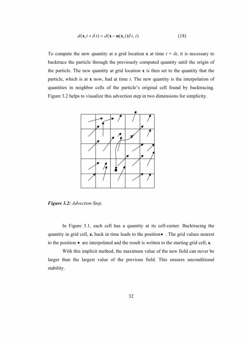
),),((),( tttdttd δδ xuxx −=+ (18)

To compute the new quantity at a grid location x at time t + δt, it is necessary to

backtrace the particle through the previously computed quantity until the origin of

the particle. The new quantity at grid location x is then set to the quantity that the

particle, which is at x now, had at time t. The new quantity is the interpolation of

quantities in neighbor cells of the particle’s original cell found by backtracing.

Figure 3.2 helps to visualize this advection step in two dimensions for simplicity.

Figure 3.2: Advection Step.

In Figure 3.1, each cell has a quantity at its cell-center. Backtracing the

quantity in grid cell, x, back in time leads to the position• . The grid values nearest

to the position • are interpolated and the result is written to the starting grid cell, x.

With this implicit method, the maximum value of the new field can never be

larger than the largest value of the previous field. This ensures unconditional

stability.

x

33

Diffusion:

Viscous fluids have a certain resistance to flow. This resistance causes

diffusion of velocity. Viscous diffusion has the following partial differential

equation:

uu 2∇=∂∂ ν

t (19)

This equation can be solved using different methods. An explicit method to solve

this equation results in the equation:

),(),(),( 2 ttttt xuxuxu ∇+=+ νδδ (20)

As in the explicit method approach in advection step, this method is unstable for

large values of kinematic viscosity, υ and time step, t. Hence, a similar implicit

approach is preferred in this diffusion step. The implicit version of equation 20 leads

to:

),(),()( 2 tttt xuxuI =+∇− δνδ (21)

where I is the identity matrix. Due to the implicit nature, this method is

unconditionally stable for large values of kinematic viscosity, υ and time step, t.

Equation 21 is also a Poisson equation like equation 12. These two equations should

be solved using the similar method.

To sum up all until this point; after adding external forces, applying diffusion

and advection, the obtained velocity vector has nonzero divergence, which should

be removed. To remove divergence, firstly, pressure field, p, should be computed by

34

solving equation 12. Then using calculated pressure field in equation 10, the

divergence free velocity vector should be found.

Poisson Equations:

There are two Poisson equations that should be solved: The pressure

equation in equation 12 and the viscous diffusion equation in equation 21. These

equations can be solved using an iterative solution technique which starts with an

approximate solution and improves it every iteration.

The Poisson equation is in the form of Ax = b, where x is a vector that

includes values of solution, b is a vector of constants and A is the matrix. In our

case, A includes the values of Laplacian operator, ∇2. In this way, we don’t need

these values beforehand. The values of ∇2 are calculated on the fly. For the equation

12, x represents velocity, u while x represents pressure, p in equation 21.

There are various iterative methods that solve Poisson equations. In this

thesis, Jacobi method, which is the simplest one, is used to solve Poisson equations

in both CPU and GPU implementations. Jacobi method starts with an initial solution

x(0) and at each step an improved solution, x(s), where subscript s represents the

iteration number. Equations 12 and 21 can be discretized with the following

formula:

βα kji

skji

skji

skji

skji

skji

skjis

kji

bxxxxxxx ,,

)(1,,

)(1,,

)(,1,

)(,1,

)(,,1

)(,,1)1(

,,

++++++= −+−+−++ (22)

where α and β are coefficients different for both equations. In pressure equation; x

represents pressure, p, b represents w⋅∇ and α = -(δx)2, β = 6. In viscous diffusion

equation; both x and b represent velocity, u and α = -(δx)2/(υδt), β = 6 + α. Since

derivations of α and β are out of scope, they are not given here.

Equation 22 is run for a number of iterations to solve both viscous diffusion

and pressure equations at each grid cell. In each iteration, the result of the previous

35

iteration is given to the next iteration as input. In this way, x(s+1) found in sth

iteration becomes x(s) in the (s+1)th iteration.

Density and Temperature Updates:

Until now, steps of external forces, advection and pressure were given for the

vector value, velocity u.

The evolution of density and temperature are given in equations 3 and 4,

respectively. As it can easily be seen, only first terms of both equations differ from

the evolution of velocity u in equation 2. In the case of velocity, velocity is advected

by itself. However, scalar values of density and temperature are advected by

velocity. Thus, in equation 18, d represents density and temperature while it

represents velocity in one of 3 directions. This term is solved for density and

temperature similarly as in velocity.

Diffusion terms in equations 3 and 4 are the same with the diffusion term in

equation 2, except for the coefficients. Thus, the iterative Jacobi method is used in

the evolution of density and temperature.

The last terms in equations 3 and 4 represent sources for density and

temperature, respectively. As in the case of velocity, in this step, the value of δt ρS

and δt TS is added to density and temperature, respectively.

Boundary Conditions:

Boundary conditions are inevitable for any differential equation problem

defined on a finite domain. Boundary conditions determine the computation of

values at the edges of the simulation domain.

In this thesis, boundary conditions are considered for both vector and scalar

values at the edges of three dimensional grid. However, for vector and scalar values

different boundary conditions are applied. Neumann boundary conditions are used

for scalar values such as density and temperature while no-slip boundary conditions

are used for velocity.

36

Neumann boundary conditions state that at a boundary, the rate of change in

the direction normal to the boundary is equal to zero. In other words, the divergence

of the scalar value across the boundary equals to zero. For example, for the left

boundary:

kjkjkjkj dd

xdd

d ,,1,,0,,1,,0 0

2=→=

−=∇

δ (23)

where δx is the grid spacing in x direction and d is density. This is the same for

temperature values. For the other boundaries, similar cases are possible.

No-slip condition states that the velocity goes to zero at the boundaries.

According to the no-slip condition, the component of velocity in parallel to the

boundary interface is zero. For example, this means that for the left boundary:

kjkjkjkj uu

xuu

,,1,,0,,1,,0 0

2−=→=

+

δ (24)

where δx is the grid spacing in x direction and u is the component of velocity in x

direction. For the left boundary, it is assumed that kjkj vv ,,1,,0 = and kjkj ww ,,1,,0 =

where v and w are the components of velocity in y and z directions, respectively.

For the other boundaries, similar cases occur for three components of

velocity, except that the components of velocity in parallel to the boundary interface

differ.

After the description of fluid flow equations used in this thesis, in the next

section, implementation of these equations in CPU is explained.

3.2 CPU Implementation

In this section, details of CPU implementation are given. Since the fluid flow

details were given in the previous section, this section focuses on the three

37

dimensional application. OpenGL API is chosen for implementation in CPU. C++

language is used as the programming language.

In CPU implementation, data is represented as a three dimensional grid. Data

represented consists of vector values such as velocity and scalar values such as

density and temperature. The discretized three dimensional grid can be seen in

Figure 3.3. The grid in the figure has dimensions of NX×NY×NZ. The grid

contains an extra layer of cells to account for the boundary conditions. For this

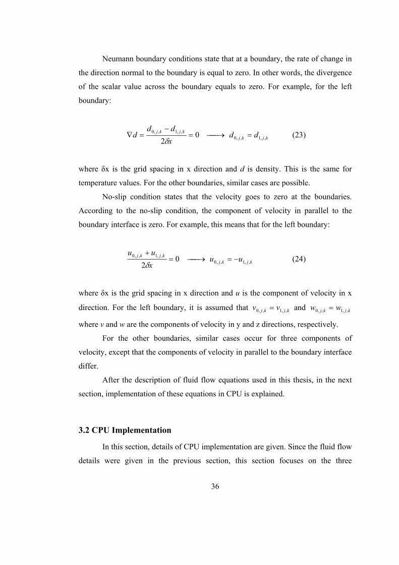
reason the actual dimensions of the grid becomes (NX+2)× (NY+2)× (NZ+2).

Figure 3.3: Discretized Three Dimensional grid.

The main structure of the implementation is as follows: We first set initial

states of velocity, temperature and density. Then, values of all these quantities are

updated at each update. For each update, first, velocity is updated, and then

temperature and density are updated in sequence. Finally, density value at each grid

cell is displayed, which visualizes the flow of smoke in the grid. The pseudo code of

the general loop is given in Figure 3.4.

38

Figure 3.4: Pseudo Code of the General Loop in CPU Implementation.

Initially, velocity, temperature and density values are set to zero. In other

words, source for any value is considered at the initial state.

When we consider the main loop, there are basically for steps. Evolution of

velocity, temperature and density are done in lines 3, 4 and 5 in Figure 3.4,

respectively. Density values are updated in line 6. This step is the rendering of the

simulations.

3.2.1 Evolution of Velocity

Evolution of velocity consists of the steps shown in Figure 3.5. Equations of

addition of forces, diffusion, projection and advection were explained in detail in the

previous section. In this section, implementation details for each step will be given.

(1) Set initial states for velocity, temperature and density

(2) While (simulating)

(3) Update velocity

(4) Update temperature

(5) Update density

(6) Display density

39

Figure 3.5: Steps in Evolution of Velocity.

These steps can be stated in the pseuodo code of the evolution of velocity.

Figure 3.6 shows the pseudo code of the velocity update step.

Figure 3.6: Pseudo Code of Velocity Update Step.

In Figure 3.6, ucurrent denotes the array of current velocity while uprevious denotes the

array of previous velocity. Since most of the operations cannot be performed in

place, temporary storage is required. For this reason, the previous velocity values

are stored. Swap operation swaps the values of current and previous values. In

Project

Add forces Diffuse

AdvectProject

(1) Add forces (ucurrent, uprevious, Tcurrent, dcurrent, dt)

(2) Swap(ucurrent, uprevious)

(3) Diffuse (ucurrent, uprevious, visc, dt)

(5) Project (ucurrent, uprevious)


(7) Advect(ucurrent, uprevious, dt)

(8) Project (ucurrent, uprevious)

40

Figure 3.6, Tcurrent and dcurrent denote array of current temperature and density values,

respectively. dt is the time step and visc is the viscosity coefficient.

Now, the details of each step are given in order. The pseudo code of the step

of addition of forces is given in Figure 3.7.

Figure 3.7: Pseudo Code of the Step of Addition of Forces.

In Figure 3.7, in line 2, vorticity confinement force is computed using the current

velocity values by solving equation 8. Fconf denotes the computed vorticity

confinement force. In the next line, this force is added to the current velocity by

simply setting ucurrent to ucurrent + dt * Fconf. In line 4, buoyant force is found using the

current velocity, density and temperature values by solving equation 5. Fbuoy denotes

the computed buoyant force. In line 5, this force is added to the current velocity as

in the case of the vorticity confinement force. In line 6, previous velocity is set to

the user-defined force. This user-defined force is such a force that simulates the

force of a virtual air blower. In line 7, this force is also added to the current velocity.

All these steps are done for each grid cell. In line 8, the array of ucurrent is updated

such that boundary conditions are applied according to the boundary conditions

mentioned in the previous section.

(1) For each grid cell

(2) Compute vorticity confinement force (ucurrent,, Fconf )

(3) Add force(ucurrent,, Fconf , dt)

(4) Compute buoyant force (ucurrent,, Fbuoy, dcurrent, Tcurrent)

(5) Add force(ucurrent,, Fbuoy , dt)

(6) Set user-defined force(uprevious)

(7) Add force(ucurrent,, uprevious , dt)

(8) Update boundary (ucurrent)

41

Diffusion step follows the addition of forces step. The pseudo code of the

diffusion step is given in Figure 3.8.

Figure 3.8: Pseudo Code of Diffusion Step.

In Figure 3.8, diffusion step is iterated for a number of

MAX_ITERATION_NUMBER. In each iteration, for each grid cell, the (s+1)th

value of the current velocity is computed using equation 22. At the end of each

iteration, the array of ucurrent is updated such that boundary conditions are applied. In

line 5, current and previous velocity arrays are swapped. This is done because

current velocity values are used as previous velocity values in the next step.

Projection step following the diffusion step is important since it forces the

velocity to be mass conserving. Visually it forces the flow of smoke to have many

vortices which produce realistic swirly-like flows. The equation details of this step

were given in the previous section. The pseudo code of the diffusion step is given in

Figure 3.9.

(1) For s = 0 to MAX_ITERATION_NUMBER-1


(3) Compute (s+1)th iteration value (ucurrent,, uprevious, vsc)



42

Figure 3.9: Pseudo Code of Projection Step. In Figure 3.9, lines 2-7 are done for each cell. First, the divergence is computed

using current velocity values. div denotes the array of divergence. In lines 3 and 4,

current and previous pressure values are initialized to zero. In lines 5-7, the

boundary conditions are applied to divergence, current pressure and previous

pressure values. In the next part of the routine, Jacobi iteration is applied for an

number of MAX_ITERATION_NUMBER. In each iteration, for each grid cell, the

(s+1)th value of the current pressure is computed using equation 22. At the end of

each iteration, the array of pcurrent is updated such that boundary conditions are

applied. In line 12, current and previous pressure arrays are swapped. This is done

because current pressure values are used as previous pressure values in the next step.

At the third part of the projection step, for each grid cell, current velocity value is


(2) Compute divergence (ucurrent,, div)

(3) Set pressure to zero (pcurrent)

(4) Set pressure to zero (pprevious)

(5) Update boundary (div)

(6) Update boundary (pcurrent)

(7) Update boundary (pprevious)

(8) For s = 0 to MAX_ITERATION_NUMBER-1


(10) Compute (s+1)th iteration value (pcurrent,, pprevious, div)

(11) Update boundary (pcurrent)

(12) Swap(pcurrent, pprevious)


(14) Compute velocity (ucurrent,, pcurrrent)

43

computed using current pressure value. This is done by subtracting the gradient of

pcurrent from ucurrent as explained in previous section.

Advection step follows the projection step. The pseudo code of the advection

step is given in Figure 3.10.

Figure 3.10: Pseudo Code of Advection Step. In Figure 3.10, advection step is summarized. For each grid cell, the current cell is

backtraced through velocity over a time –dt. inew, jnew, knew denote the endpoint cell

found in this backtracing. The current velocity of the current cell is set to the

interpolation of velocity values in the neighbor cells of the cell(inew, jnew, knew).

Finally, boundary conditions are applied to the current velocity values.

Advection step is again followed by the projection step. This is done to force

the velocity to be mass conserving.

3.2.2 Evolution of Temperature and Density

Evolution of temperature and density values resembles to the evolution of

velocity. Evolution of scalar values such as density and temperature consists of the

steps shown in Figure 3.11. As it can be seen, the difference is the absence of the

projection step that appears in Figure 3.5. Projection step forces the vector value to

be mass conserving so it is not required in the evolution scalar values.


(2) Traceback (uprevious, -dt, inew, jnew, knew)

(3) Compute interpolation (ucurrent,, uprevious, inew, jnew, knew)


44

Figure 3.11: Steps in Evolution of Scalar Values.

These steps can be stated in the pseudo code of the evolution of scalar

values. Figure 3.12 shows the pseudo code of the density update step. Since the

temperature update step is the same, it will not be given separately.

Figure 3.12: Pseudo Code of Density Update Step.

In Figure 3.6, dcurrent denotes the array of current density while dprevious denotes the

array of previous density. Since most of the operations cannot be performed in

place, temporary storage is required. For this reason, the previous density values are

stored. Swap operation swaps the values of current and previous values as in the

case of velocity. dt is the time step and visc is the viscosity coefficient.

The details of diffusion and advection step were given in the evolution of

velocity, these steps are not explained again. All velocity values in those pseudo

codes are substituted with density and temperature values. Here, only the pseudo

code of the step of addition of sources is given in Figure 3.13.

Add sources Diffuse Advect

(1) Add sources (dcurrent, dprevious, dt)

(2) Swap(dcurrent, dprevious)

(3) Diffuse (dcurrent, dprevious, visc, dt)

(4) Swap(dcurrent, dprevious)

(5) Advect(dcurrent, dprevious, dt)

45

Figure 3.13: Pseudo Code of the Step of Addition of Sources.

In Figure 3.13, in line 2, previous density is set to the user-defined source. This

user-defined source is such a source that simulates the source of a virtual air blower.

In line 3, this force is added to the current density by simply setting dcurrent to dcurrent

+ dt * dprevious. All these steps are done for each grid cell. In line 4, the array of

dcurrent is updated such that boundary conditions are applied according to the

boundary conditions mentioned in the previous section. After this step, diffusion and

advection steps are applied to density values.

After velocity, temperature and density values are updated, current density

values are rendered using OpenGL API commands. The details of rendering are

explained in Section 3.4.

3.3 GPU Implementation

GPU has many advantages over CPU in general-purpose computations. This

is the natural consequence of the support for programmability at vertex and

fragment levels and IEEE 32 bits float precision throughout the whole pipeline. In

GPU implementation, basically, the whole computation domain is mapped directly

to texture memory and fragment programs are used to solve the fluid flow equations

described before.


(2) Set user-defined source(dprevious)

(3) Add force(dcurrent,, dprevious , dt)

(4) Update boundary (dcurrent)

46

In this section, before the explanation of GPU implementation details of

three dimensional smoke simulation, the differences between CPU and GPU

implementations will be given.

3.3.1 Differences between CPU and GPU Implementations

Data Representation:

The smoke simulation in this thesis is three dimensional. Thus, data is

represented on a three dimensional grid. As explained in the previous section, the

natural representation for this grid on CPU is an array. The analog of an array on

GPU is a texture. Textures on GPU are not as flexible as arrays on CPU. However,

their flexibility is improving with the evolution in graphics hardware. Textures on

current GPUs support all the basic operations necessary to implement a three

dimensional smoke simulation. Since textures usually have four color channels, they

provide a natural data structure for vector data types with components up to four.

In this simulation, vector values such as velocity and scalar values such as

temperature and density are stored in textures. For velocity values, three channels of

textures are occupied by the three components of RGBA 4 channels of a single

texel. In the case of scalar values such as temperature and density, we can exploit

the fact that the same operations are done to compute these values. Owing to this

exploitation, to reduce the number of passes on GPU at the fragment level, we pack

scalar values into RGBA 4 channels of a single texel as in [47]. This is an important

advantage of textures, which halves the number of rendering passes done for the

calculation of scalar values.

Different from two dimensional fluid simulations, one of the difficulties in

three dimensional fluid simulations is the representation of three dimensional grid as

a texture. This can be done by different methods such as using a stack of 2D

textures, or 3D textures. In these methods volume must be updated by slice by slice,

requiring texture copies or context switches. Another method is using flat 3D

textures, which we utilize in the GPU implementation. A flat 3D texture is a 2D

47

texture that contains the tiled slices of a three dimensional volume [48], as shown in

Figure 3.14. In the figure, outside parts of inner quads represent the boundary cells

of each slice. The quads in the bottom left and the top right corners are the boundary

slices of the volume along the slicing axis.

Figure 3.14: Comparison of 3D Textures and Flat 3D Textures. (a) 3D Texture (b) Corresponding Flat 3D Texture (Inspired by [48]).

The advantage of 3D textures over flat 3D textures is the easy addressing in

3D textures. However, in flat 3D textures, offsets for neighbor cells along the slicing

axis and boundary cells should be computed beforehand. On the other hand, flat 3D

textures have the advantage of being updated in a single render pass. For the entire

volume, only one texture update is required. This is the main advantage of flat 3D

textures. In this thesis, flat 3D textures are used for the representation of three

dimensional volume as a texture. For flat 3D textures, the interior of each slice is

rendered as a quad, and the boundaries are rendered as lines. Different fragment

programs are used to achieve this.

As well as data representation, the read operation differs on GPU. On CPU,

the array is read using an offset or index. However, on GPU, textures are read using

a texture lookup.

N

. 7

. .

0 0 1 2 3

4 5 6 7

N

Line Primitives Quad Primitives

48

Processing Model:

In CPU implementation of the simulation, all steps in the algorithm are

performed by looping. To iterate over each grid cell, three nested loops are used. At

each cell, the same computation is performed. However, the processing of algorithm

is different on GPU. Current fragment shader does not support the loop operation

over each texel in a texture. However, the fragment pipeline is designed to perform

identical computations at each fragment. The fragment pipeline is designed in the

way that it appears as if there is a processor for each fragment and all fragments are

updated simultaneously. This is the natural consequence of parallelism of GPU.

The main algorithm flow for velocity values on GPU is shown in Figure

3.15. It is very similar to the flow of velocity update in Figure 3.5 except that here,

instead of array texture is updated. In Figure 3.16, the main algorithm flow for

scalar values such as density and temperature is seen. Here, one texture is used to

store both values.

Figure 3.15: Algorithm Flow for Velocity Texture on GPU.

Project Advect

Project

Add forces Diffuse

49

Figure 3.16: Algorithm Flow for Texture of Scalar Values on GPU.

To sum up, computation on CPU occurs inside nested loops over an array,

while fragment programs are applied to each fragment on GPU.

Data Computation:

In CPU implementation, arrays are used to represent the three dimensional

grid. These arrays are read and written in a trivial way. However, implementation of

data computation on GPU is not that easy. On GPU, the output of fragment

processors is always written to the frame buffer. Frame buffer can be assumed as a

two-dimensional array that cannot be directly read. There are two ways to get the

contents of the frame buffer into a texture that can be read:

1. Copy-to-texture (CTT) transfers data from the frame buffer to a texture.

Figure 3.17 shows the copy-to-texture mechanism.

CPU VertexProgram

FragmentProgram

FrameBuffer

Figure 3.17: Copy-to-Texture Mechanism.

Add sources Diffuse Advect

50

2. Render to texture (RTT) renders directly into a texture. The texture is

used as the frame buffer so that the GPU can write directly to it. Figure

3.18 shows the render-to-texture mechanism.

CPU VertexProgram

FragmentProgram

Figure 3.18: Render-to-Texture Mechanism. CTT and RTT function equally well. However, they have different performances. In

CTT, transfer does not cross GPU-CPU boundary. But, it is not very flexible and is

still slow. In RTT, transfer does not cross GPU-CPU boundary like in CTT. Since

data is transferred directly to the texture, it is faster than CTT. For this reason, in our

GPU implementation, RTT is used to increase performance.

3.3.2 Implementation Details

After explaining the differences between CPU and GPU implementations,

details of GPU implementation presented given in this subsection.

The pseudo code of the main algorithm in GPU implementation is given in

Figure 3.19.

51

Figure 3.19: Pseudo Code of the Main Loop on GPU Implementation.

In the main loop, first OpenGL initialization is done. Next, an offscreen

buffer in GPU memory is created to handle RTT. Then, Cg vertex and fragment

shader programs are initialized. Next, the initial grid data is loaded to the offscreen

buffer as textures. All these are done initially only once. Lines 5-7 are done in each

frame update. In each frame, computations of fluid flow are performed on textures

in offscreen buffer using ping-pong approach. This step is followed by reading back

density texture into CPU memory. Finally, density values are rendered to visualize

smoke flow in three dimensional space.

Setting up OpenGL:

OpenGL extension functions are required in the implementation. Thus, in

step of setting up OpenGL, it is first checked if all neccessary extensions are

supported. Then, pointers for extension functions are taken.

Creating Offscreen Buffer:

As described before, for performance reasons, rendering to texture is

preferred. The pBuffer extension to OpenGL allows the use of offscreen floating

(1) Setup OpenGL

(2) Create offscreen buffer

(3) Setup CG

(4) Load data to offscreen buffer

In each frame

(5) Perform computations on textures

(6) Readback density data from the frame buffer to CPU

(7) Render density values

52

point rendering targets. There is an important detail for pBuffers that should be

considered. pBuffers are either read-only or write-only. When bound as an input

texture, a pBuffer is read-only. On the other hand, a pBuffer is write-only when

bound as render target. Unfortunately, we need to read and update data in each step.

There are two solutions to this problem: Using two pBuffers or using one double-

buffered pBuffer. In the former case, switches should be done between the OpenGL

contexts of pBuffers. This is an expensive solution since switching the OpenGL

context requires a flush of the graphics pipeline. For this reson, it is more convenient

to use one double-buffered pBuffer. A double-buffered pBuffer is a single buffer,

with two surfaces. One surface is for reading from and the other is for writing to.

Render to texture approach with double-buffered pBuffer is used in this

implementation, which increases performance. In the first step, the results are

rendered into a buffer which is then used as an input texture for the next step

without any actual copying of data or anything else that would inhibit high

performance. This process is known as the ping-pong approach.

In the initialization of pBuffer, a double-buffered offscreen rendering target

with four channels of 32 bit precision each, supporting RTT approach and access to

its data with the texRECT extension instead of the tex2D texture lookup.

Rectangular textures differ from 2D textures. Their coordinates are in the range of

[0, texWidth] × [0, texHeight] where texWidth is the width and texHeight is the

height of texture. On the other hand, the coordinates are in the range of [0, 1] × [0,

1]. Thus, using rectangular textures is what we need.

After creating the pBuffer in the mode and size our implementation requires,

something more complicated should be done. The created buffer is turned into the

current OpenGL render target. Then, since a one to one mapping of the values in the

vectors, the viewport and textures will be used, a simple one-to-one two dimensional

orthographic projection is setup. The pBuffer is then bound as a texture. As it was

stated before, the pBuffer has its own context, so everything done after turning the

buffer’s OpenGL render target affects this context until turning off this render target

53

to the actual OpenGL render target. For the details of RTT using pBuffers, please

refer to [30].

Setting up Cg:

To be able to use Cg, some initialization should be done. Pseudo code of Cg

setup is shown in Figure 3.20.

Figure 3.20: Pseudo Code of Cg Setup. First, in line 1, an error callback function is set for understanding errors. Next, Cg

context that contains multiple Cg programs is created. In lines 3-4, the best available

profile for vertex or fragment programs depending on the available OpenGL

extensions are provided. Then each vertex and fragment shader program is created

from the functions in different files. After creation, each program is compiled and

loaded.

In our GPU implementation, one vertex shader program is used. The Cg

code of this vertex shader program is given in Figure 3.21.

(1) cgSetErrorCallback(handleCgError)

(2) context = cgCreateContext()

(3) vertexProfile = cgGLGetLatestProfile(CG_GL_VERTEX)

(4) fragmentProfile= cgGLGetLatestProfile(CG_GL_FRAGMENT)

(5) for each vertex and fragment shader program

(6) program = cgCreateProgramFromFile (context,

CG_SOURCE, fileName,

vertexProfile, program_name, NULL)

(7) cgCompileProgram(program)

(8) cgGLLoadProgram(program)

54

Figure 3.21: Cg Code of Vertex Shader Program. In line 4 in Figure 3.21, viewspace transformation is performed. modelViewMatrix

is a parameter set by the three dimensional application. inpos is a three dimensional

vertex data. outpos is the viewspace transformed data. outpos is given to the

fragment shader programs as input showing the texel coordinates. Thus, in texture

lookups, this parameter is used.

There are many different fragment shader programs for the computation of

fluid flow equations. There is one common thing for fragment shader programs.

Each fragment shader program takes at least one rectangle texture of type

samplerRECT and the proper fragment coordinates through the WPOS binding

semantics for the fragment as parameters. As a result, these programs calculate the

result which is returned as a color value.

Loading Data to Offscreen Buffer:

In this step, upload the starting values defined earlier in an array on CPU

memory are rendered to the offscreen buffer before the processing on GPU.

Performing Computations on Textures:

This step is the most important in the main GPU implementation. All

computations on textures are performed in this step. The pseudo code of this step is

given in Figure 3.22.

(1) void main (in float4 inpos: POSITION,

(2) out float4 outpos: WPOS,

(3) const uniform float4x4 modelViewMatrix)

{

(4) outpos = mul (modelViewMatrix, inpos);

}

55

Figure 3.22: Pseudo Code of Performing Computations on Textures.

(1) begin rendering to offscreen texture

(2) enable Cg vertex profile

(3) enable Cg fragment profile

(4) bind Cg vertex program

(5) set Cg vertex program parameter

// Velocity update starts

(6) process (addForces fragment program)

(7) process (diffuse fragment program)

(8) process (projection fragment program)

(9) process (advection fragment program)

(10) process (projection fragment program)

// Velocity update ends

// Density and temperature update starts

(11) process (addSources fragment program)

(12) process (diffuse fragment program)

(13) process (advection fragment program)

// Density and temperature update ends

(14) disable Cg vertex profile

(15) disable Cg fragment profile

(16) end rendering to offscreen texture

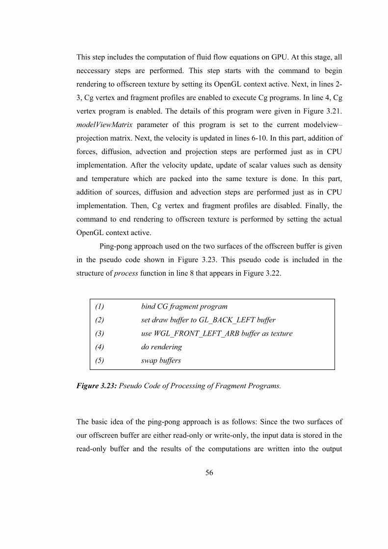
56

This step includes the computation of fluid flow equations on GPU. At this stage, all

neccessary steps are performed. This step starts with the command to begin

rendering to offscreen texture by setting its OpenGL context active. Next, in lines 2-

3, Cg vertex and fragment profiles are enabled to execute Cg programs. In line 4, Cg

vertex program is enabled. The details of this program were given in Figure 3.21.

modelViewMatrix parameter of this program is set to the current modelview–

projection matrix. Next, the velocity is updated in lines 6-10. In this part, addition of

forces, diffusion, advection and projection steps are performed just as in CPU

implementation. After the velocity update, update of scalar values such as density

and temperature which are packed into the same texture is done. In this part,

addition of sources, diffusion and advection steps are performed just as in CPU

implementation. Then, Cg vertex and fragment profiles are disabled. Finally, the

command to end rendering to offscreen texture is performed by setting the actual

OpenGL context active.

Ping-pong approach used on the two surfaces of the offscreen buffer is given

in the pseudo code shown in Figure 3.23. This pseudo code is included in the

structure of process function in line 8 that appears in Figure 3.22.

Figure 3.23: Pseudo Code of Processing of Fragment Programs.

The basic idea of the ping-pong approach is as follows: Since the two surfaces of

our offscreen buffer are either read-only or write-only, the input data is stored in the

read-only buffer and the results of the computations are written into the output

(1) bind CG fragment program

(2) set draw buffer to GL_BACK_LEFT buffer

(3) use WGL_FRONT_LEFT_ARB buffer as texture

(4) do rendering

(5) swap buffers

57

buffer. The input data is bound as a texture. Reading from this texture and writing

into the output buffer is the first step to be performed. This is all about ping step.

Then, the role of the two buffers is swapped. The output buffer that is just rendered

to becomes the new input buffer, again as a texture. This is the reason for calling the

whole process “render to texture”. The former input buffer can be overwritten with

the results of this iteration step since it is not needed any more. Then the buffers are

swapped again and start over.

In Figure 3.23, in line 1, the Cg fragment program such as addForces is

bound to be executed. The draw buffer is set to GL_BACK_LEFT buffer and

WGL_FRONT_LEFT_ARB buffer is set as input texture. In this way, the previously

rendered texture (i.e. texture with the values computed in the previous step) is used

as input texture. Then, in line 4, a viewport-sized quad is rendered. This causes the

rasterizer to create a fragment for each pixel in the viewport. The quad basically

serves as a data stream generator for the fragment program which gets executed

independently for each of these fragments. The texture coordinates of the data

texture are set to a one-to-one mapping between pixels and texels. In this way it is

possible to access the right positions in both the input and the output buffer, in each

iteration. In line 5, the buffers for both input and output buffer are swapped.

GL_BACK_LEFT buffer becomes GL_FRONT_LEFT buffer while

WGL_FRONT_LEFT_ARB buffer becomes WGL_BACK_LEFT_ARB buffer. This is

necessary for the pong step of ping-pong approach.

Using ping-pong approach, the number of rendering passes decreases, which

increases the performance.

For instance, in Figure 3.24, addForce Cg fragment program code is given.

58

Figure 3.24: addForce Cg Fragment Program Code.

Reading Back Density Data from Frame Buffer to CPU:

At the end of the processing on GPU, data is read back from the texture

which contains density and temperature values to CPU.

Rendering Density Values:

Density values read back in the previous step are rendered using OpenGL

API commands. The details of rendering are explained in Section 3.4.

float4 addForce ( in half2 screen : WPOS, // grid coordinates

uniform samplerRECT texture1, // first texture

uniform samplerRECT texture2, // second texture

uniform float timeStep

) : COLOR

{

float4 OUT;

half2 ocoords = screen.xy;

float4 val1 = f4texRECT (texture1, ocoords);

float4 val2 = f4texRECT (texture2, ocoords);

OUT = val1 + val2 * timeStep;

return OUT;

}

59

3.4 Rendering

Density values obtained for each grid cell are rendered in order to visualize

the flow of smoke. In this thesis, rendering is performed using texture based volume

rendering methods. Since the main focus of this thesis is on the improvement of the

performance of fluid flow computations on GPU, rendering will not be explained in

much detail. In this part, texture based volume rendering methods used in the

visualization of this smoke simulation will be overviewed.

Texture based methods utilize the hardware support of texture units for

interpolation in sampling of volume data. Therefore, these techniques are faster than

the software based volume rendering methods. Texture based methods are classified

as 2D texture based methods and 3D texture based methods. Both methods are

handled in this thesis.

2D texture based volume rendering methods work by rendering a stack of

texture mapped quads almost perpendicular to the view direction with each texture

containing an axis-aligned slice of the 3D data. For this reason, as the view direction

changes, the direction and size of the rendered slices change so that they should be

rendered along the axis that is most parallel to the view direction. The axis that is

most parallel to the view direction is selected by transforming the three principal

axes with the view rotation matrix. Then, the vector of each transformed axis is

dotted with the view vector which is in –z direction (0, 0, -1). The axis with the

largest dot product is decided to be the axis most parallel with the view direction. In

Figure 3.25, 2D slices are defined parallel to ZX plane and each slice is rendered as

a textured polygon, from back to front (definition of front and back changes

according to the view direction). A blend operation is performed at each slice. In

this thesis, GL_SRC_ALPHA is used as source blending factor, while

GL_ONE_MINUS_SRC_ALPHA is used as destination blending factor.

60

Figure 3.25: 2D Axis-aligned Texture Slices.

Today, many graphics boards support 2D texture mapping hardware.

Therefore, utilizing the texture hardware for 2D texture volume rendering is

advantageous. Moreover, rendering with 2D textures can be realized with high

performance. The drawback of 2D textures is that the slice polygons can't always be

perpendicular to the view direction. Thus, as the view directions changes, slices

should again be aligned along the axis that is most parallel to the view direction.

Furthermore, it is not possible to obtain high quality image with 2D textures.

With a recent addition to graphics cards, the use of 3D textures has been

introduced. In this method, a complete texture volume is downloaded to the graphics

card and 3D texture coordinates are used instead of 2D coordinates to lookup into

the volume. This is a more natural method for volume rendering. However, it is

implemented less efficiently than 2D textures.

In view-aligned 3D texture based volume rendering method, all the texture

slices are arranged parallel to the view plane. For this reason, using 3D textures for

volume rendering is more desirable than 2D textures. Figure 3.26, shows the

arrangement of texture slices according to the view direction.

z

y

x

61

Figure 3.26: Arrangement of Texture Slices According to View Direction.

The intersection points of the slices are calculated and the according point index

sequence is found. Then, the slices are rendered using OpenGL 3D texture mapping

API calls.

One of the advantages of 3D textures over 2D textures is the generation of

high quality images. Moreover, the texture slices can be oriented according to the

view direction. However, 3D texture based volume rendering method is slower than

2D texture based volume rendering method. Figure 3.27 shows a closer look to two

different smoke images with 2D axis-aligned textures slices and 3D view-aligned

textures slices, respectively.

Figure 3.27 Smoke Images Rendered with Different Methods. (a) 2D Axis-aligned Textures Slices, (b) 3D View-aligned Textures Slices.

View Directio

z

y

x

62

CHAPTER 4

DISCUSSION AND RESULTS

All experiments have been performed on a PC with Pentium 4 3.0 GHz and 1

GB main memory. The graphics chip is GeForce FX 5700 with 256 MB video

memory. The operating system is Windows XP. Experiments have been done on

both CPU and GPU to compare the computation times of fluid mechanics equations.

All the computations in this thesis are based on 32-bit float precision to make it

suitable for real-world problems.

Flat 3D textures are used to represent data on GPU. Figure 4.1 shows the flat

3D texture of a flowing smoke in upward direction in a grid of 16×32×16 voxels.

As it can be seen from the figure, there are 18 slices. Since we apply boundary

conditions for both all scalar values such as density and temperature and vector

values, we add extra two slices for extra boundary cells in z direction.

Figure 4.1: Flat 3D Texture of Flowing Smoke in a Grid of 16×32×16 Voxels.

63

Figure 4.2 shows four sequential scenes of smoke flowing in a grid of

16×32×16 voxels. In the scene, there is a density source at the bottom of the grid

and the velocity is mainly flowing in upward direction, which simulates an air

sprayer at the bottom. In Figure 4.2 (a), smoke starts to release from a source of

virtual air sprayer at the bottom and in Figure 4.2 (b)-(c), smoke continues to flow

up with the fluid flow effects. In Figure 4.2 (d), smoke touches the top boundary of

the grid and the application of boundary conditions are seen.

64

Figure 4.2: Flowing of Smoke in a Grid of 16×32×16 Voxels in Upward Direction in Movement Sequence of (a), (b), (c) and (d).

65

As it can be seen in these figures, the smoke simulation is physically

realistic. During rendering process, we don’t use shading effects. Thus, if we add the

shading effects, the whole simulation will look much more realistic.

The experiments have been done on grids of different sizes. Table 4.1 gives

the comparison of the performances of the same algorithm run on GPU and CPU on

the same platform. To achieve reliable test results, on both CPU and GPU

implementation, all steps are included and the same number of iterations is executed

to solve Poisson equations. The comparison results in Table 4.1 show that with the

grid of dimensions 16x16x16, the performance of CPU is better than GPU. This is

because of the high proportion of messages passed between CPU and GPU in

fragment shader programs. However, with the increase in grid size, the proportion of

messages passed between CPU and GPU in fragment shader programs decreases.

Supporting this idea, with the increase in grid size, performance on GPU exceeds

performance on CPU about 9 times in Table 4.1. Since the texture size is limited

with GPU video memory, the implementation could not be tested on grids with

larger sizes.

Table 4.1 Comparison of Performance on CPU and GPU

Consequently, the experiments on CPU and GPU prove the performance of

GPU on pyhsically based calculations such as smoke simulations.

Grid Dimensions

Average

CPU Time

(ms)

Average

GPU Time

(ms)

SpeedUp

16x16x16 66 97 0.68

32x32x32 667 344 1.94

64x64x64 11989 2128 5.63

128x128x128 139867 14790 9.46

66

CHAPTER 5

CONCLUSION AND FUTURE WORKS

In this thesis, three dimensional simulation of smoke was performed on both

CPU and GPU. The literature about fluid mechanics and GPU programming was

surveyed in detail.

For the physical simulation of smoke behavior, Navier-Stokes equations

were solved using a semi-Lagrangian unconditionally stable method. Owing to the

parallelism in graphics hardware, smoke simulation performed on GPU runs

significantly faster than the corresponding CPU implementation. The results show

the difference in performance of computations reliably since both CPU and GPU

implementations used the same steps and number of iterations for Poisson equations.

CPU and GPU implementations differ from each other in some aspects.

Representation is the first of all. In CPU implementation, grid cells are represented

in an array while in GPU implementation, data is stored in textures, the analogy of

arrays on GPU. For the representation of three dimensional data on GPU, flat 3D

textures, in which slices of volume are arranged in two dimensions, were used. The

use of flat 3D textures reduces the number of rendering passes, since the whole

volume data is processed in only one render.

Three dimensional data consists of different scalar attributes such as density,

and vector attributes such as velocity. Scalar values such as temperature and density,

which are very similarly processed, packed into a single RGBA-4 channel texel at

fragment level. In this way, the number of rendering passes is decreased by reducing

the number of textures to be processed. Furthermore, to improve the performance of

GPU implementation, double-buffered offscreen floating point rendering targets

67

were utilized, which decreases context switches. Since context switches are very

expensive, the decrease in context switches increases performance. Ping-pong

approach which utilizes double buffers of rendering textures was also used. With

this approach, offscreen texture can be used as input and output textures. This is

another performance increasing issue implemented in this three dimensional smoke

simulation on GPU.

With the implementation of all methods explained above, the results satisfied

the expectations at the end of the experiments done on different sized grids, which is

very satisfying.

5.1 Future Works

We are currently working on accelerating fluid flow further. This may be

achieved by decreasing the number of passes further and optimizing the GPU

instructions. Since the computations mostly rely on fragment programs, the message

passing scheme between CPU and GPU can be balanced so that the fluid flow is

accelerated.

We would like to further extend our work to simulate other fluids such as

liquids and fire. Moreover, in the near future we would like to transfer rendering

part to GPU.

Addition of arbitrary complex obstacles [47] is another issue that we would

like to implement in our smoke simulation.

Due to the limitation of texture memory on graphics card, the method

implemented on GPU is not suitable for large-scale fluid flow problems. In the

future, texture compression may be a solution for large-scale problems.

68

REFERENCES

[1] W. T. Reeves, “Particle Systems - A Technique for Modelling a Class of Fuzzy Objects”, Proceedings of SIGGRAPH ’83, vol. 17, pp. 359-376, 1983. [2] S. Clavet, P. Beaudoin, and P. Poulin, “Particle-Based Viscoelastic Fluid Simulation”, Eurographics/ACM SIGGRAPH Symposium on Computer Animation ’05, pp. 219-228, 2005. [3] N. Foster and D. Metaxas, “Realistic Animation of Liquids”, Graphical Models and Image Processing, vol. 58, pp. 471- 483, 1996. [4] Y. Liu, X. Liu, H. Zhu , E. Wu, “Physically Based Fluid Simulation in Computer Animation”, to appear in Journal of Computer-Aided Design and Computer Graphics, 2005. [5] J. Stam, “Stable Fluids”, Proceedings of SIGGRAPH ’99, pp121-128, 1999. [6] Official GPGPU Website, http://www.gpgpu.org, last access date August 2005. [7] G. Miller and A. Pearce, “Globular Dynamics: A Connected Particle System for Animating Viscous Fluids”, Computers and Graphics, vol. 13(3), pp. 305-309, 1989. [8] J. F. O'Brien and J. K. Hodgins, “Dynamic Simulation of Splashing Fluids”, Proceedings of Computer Animation ’95, pp. 198-208, 1995. [9] J. Stam and E. Fiume, “Depicting Fire and Other Gaseous Phenomena Using Diffusion Processes”, Proceedings of SIGGRAPH ’95, pp. 129–136, 1995. [10] L. B. Lucy, “A Numerical Approach to the Testing of the Fission Hypothesis”, Astronomical Journal, vol. 82, pp. 1013-1024, 1977. [11] R. A. Gingold, J. J. Monaghan, “Smoothed Particle Hydrodynamics - Theory and Application to Nonspherical Stars”, Monthly Notices of Royal Astronomical Society, vol. 181 (1977), 375-389, 1977.

69

[12] M. Desbrun and M. P. Gascuel, “Smoothed Particles: A New Paradigm for Animating Highly Deformable Bodies”, Computer Animation and Simulation ’96, pp. 61-76, 1996. [13] M. Müller, D. Charypar and M. Gross, “Particle-Based Fluid Simulation for Interactive Applications”, Proceedings of SIGGRAPH/Eurographics Symposium on Computer Animation ’ 03, pp. 154-159, 2003. [14] M. Müller, R. Keiser, A. Nealen, M. Pauly, M. Gross, M. Alexa, “Point Based Animation of Elastic, Plastic and Melting Objects”, Proceedings of SIGGRAPH/ Eurographics Symposium on Computer Animation ’04, pp. 141-151, 2004. [15] S. Premoze, T. Tasdizen, J. Bigler, A. Lefohn and R. Whitaker, “Particle-Based Simulation of Fluids”, Computer Graphics Forum 22, vol. 3, pp. 401-410, 2003. [16] R. Fedkiw, J. Stam and H.W. Jensen, “Visual Simulation of Smoke”, Proceedings of SIGGRAPH ’01, pp.15-22, 2001. [17] Y. Liu, X. Liu and E. Wu, “Real-Time 3D Fluid Simulation on GPU with Complex Obstacles”, Proceedings of Pacific Graphics ’04, pp. 247-256, 2004. [18] M. Kass and G. Miller, “Rapid, Stable Fluid Dynamics for Computer Graphics”, Proceedings of SIGGRAPH ’90, vol. 24, pp. 49-57, 1990. [19] J. X. Chen, N. Lobo, C. E. Hughes and J. M. Moshell, “Real-Time Fluid Simulation in a Dynamic Virtual Environment”, IEEE Computer Graphics and Applications, vol. 17(3), pp. 52-61, 1997. [20] J. Stam and E. Fiume, “Turbulent Wind Fields for Gaseous Phenomena”, Proceedings of SIGGRAPH ’93, pp. 369–376, 1993. [21] N. Foster, D. Metaxas, “Modeling the Motion of a Hot, Turbulent Gas”, Proceedings of SIGGRAPH ’97, pp. 181- 188, 1997. [22] R. Fedkiw, J. Stam and H. W. Jensen, “Visual Simulation of Smoke”, Proceedings of SIGGRAPH ’01, pp. 23-30, 2001. [23] D. Enright, S. Marschner and R. Fedkiw, “Animation and Rendering of Complex Water Surfaces”, Proceedings of SIGGRAPH ’02, pp. 736-744, 2002. [24] N. Foster and R. Fedkiw, “Practical Animation of Liquids”, Proceedings of SIGGRAPH ’01, pp. 15-22, 2001.

70

[25] D. Q. Nguyen, R. Fedkiw and H. W. Jensen, “Physically Based Modeling and Animation of Fire”, Proceedings of SIGGRAPH ’02, pp. 703-707, 2002. [26] N. Rasmussen, D. Q. Nguyen, W. Geiger and R. Fedkiw, “Smoke Simulation for Large Scale Phenomena”, Proceedings of SIGGRAPH ’03, pp. 703-707, 2003. [27] F. Losasso, F. Gibou and R. Fedkiw, “Simulating Water and Smoke with an Octree Data Structure”, Proceedings of SIGGRAPH ’04, pp. 457-462, 2004. [28] T. G. Goktekin, A. W. Bargteil and J. F. O’Brien, “A Method for Animating Viscoelastic Fluids”, Proceedings of SIGGRAPH ’04, pp. 463-468, 2004. [29] R. Fernando, M. J. Kilgard, “The Cg Tutorial: The Definitive Guide to Programmable Real-Time Graphics”, Addison-Wesley Professional, 2003. [30] NVidia Developer Home Page, http://developer.nvidia.com, last access date August 2005. [31] The RenderMan Interface Specification, https://renderman.pixar.com/products/rispec/, last access date August 2005. [32] M. Olano and A. Lastra, “A Shading Language on Graphics Hardware: The PixelFlow Shading System”, Proceedings of SIGGRAPH ’98, pp. 159-168, 1998. [33] K. Proudfoot, W. R. Mark, S. Tzvetkov, and P. Hanrahan, “A Real-Time Procedural Shading System for Programmable Graphics Hardware”, Proceedings of SIGGRAPH ’01, pp. 159-170, 2001. [34] Microsoft DirectX Home Page, http://www.microsoft.com/windows/directx, last access date August 2005. [35] Official OpenGL Website, http://www.opengl.org, last access date August 2005. [36] A. J. Chorin and J. E. Marsden, “A Mathematical Introduction to Fluid Mechanics", New York: Springer-Verlag, 1993. [37] B. Jobard, G. Erlebacher and M. Y. Hussaini, “Hardware Accelerated Texture Advection for Unsteady Flow Visualization”, IEEE Visualization, pp. 155-162, 2000. [38] D. Weiskopf, M. Hopf, and T. Ertl, “Hardware-Accelerated Visualization of Time-Varying 2D and 3D Vector Fields by Texture Advection via Programmable

71

Per-Pixel Operations”, Workshop on Vision, Modeling, and Visualization VMV, pp. 439-446, 2001. [39] W. Li, X. Wei and A. Kaufman, “Implementing Lattice Boltzmann Computation on Graphics Hardware”, The Visual Computer, vol. 19, pp. 444-456, 2003. [40] W. Li, Z. Fan, X. Wei and A. Kaufman, “GPU-Based Flow Simulation with Complex Boundaries”, Technical Report 031105, Computer Science Department, SUNY at Stony Brook, 2003. [41] M. J. Harris, G. Coombe, T. Scheuermann and A. Lastra, “Physically-Based Visual Simulation on Graphics Hardware”, Proceedings of Graphics Hardware, pp.109-118, 2002. [42] J. Krüger and R.Westermann, “Linear Algebra Operators for GPU Implementation of Numerical Algorithms”, Proceedings of SIGGRAPH, pp. 908-916, 2003. [43] J. Bolz, I. Farmer, E. Grinspun and P. Schröoder, “Sparse Matrix Solvers on the GPU: Conjugate Gradients and Multigrid”, Proceedings of SIGGRAPH, pp. 917-924, 2003. [44] N. Goodnight, C. Woolley, D. Luebke and G. Humphreys, “A Multigrid Solver for Boundary Value Problems Using Programmable Graphics Hardware”, Proceedings of Graphics Hardware, pp.102-111, 2003. [45] M. J. Harris, W. V. Baxter III, T. Scheuermann and A. Lastra, “Simulation of Cloud Dynamics on Graphics Hardware”, Proceedings of Graphics Hardware, pp. 92-101, 2003. [46] E. Wu, Y. Liu and X. Liu, “An Improved Study of Real-Time Fluid Simulation on GPU”, Journal of Computer Animation and Virtual World (CASA2004), vol. 15 (no. 3-4), John Wiley & Sons, pp.139-146, 2004. [47] Y. Liu, X. Liu and E. Wu, “Real-Time 3D Fluid Simulation on GPU with Complex Obstacles”, ACM Workshop on General-Purpose Computing on Graphics Processors (GP2), 2004. [48] M. J. Harris, “Real-Time Cloud Simulation and Rendering”, Ph.D. dissertation, University of North Carolina at Chapel Hill, 2003.

72

[49] C. Scheidegger, J. Comba, R. Cunha “Navier-Stokes on Programmable Graphics Hardware using SMAC”, Proceedings of XVII SIBGRAPI - II SIACG 2004, pp. 308-315, 2004.

smoke simulation on programmable graphics hardware...

Documents