smc with disturbance observer for a linear belt- drive · smc with disturbance observer for a...
TRANSCRIPT

SMC with Disturbance Observer for a Linear Belt-Drive
Aleš Hace, Member, IEEE, Karel Jezernik, Senior Member, IEEE, Asif Šabanović, Senior Member, IEEE
Abstract
Accurate position tracking control in a belt-driven servomechanism can experience vibrations and large
tracking errors due to compliance and elasticity introduced by force transmission through the belt and
nonlinear friction phenomenon. In this paper, a new control algorithm based on sliding mode control that
is able to deal with these problems is proposed. In order to further optimize position tracking performance
the control scheme has been extended by an asymptotic disturbance observer. It has been proven that
robust and vibration-free operation of a linear belt-driven system can be achieved. The experiments
presented in the paper show improved position tracking error response while maintaining vibration
suppression.
Keywords motion control, sliding mode control, disturbance observer, timing-belt drive, vibration suppression Corresponding author:
Dr. Aleš Hace Faculty of Electrical Engineering and Computer Science University of Maribor Smetanova ulica 17, SI-2000 Maribor, Slovenia phone: +386 2 2207307 fax: +386 2 2207315 email: [email protected]
Aleš Hace and Karel Jezernik are with the Institute of Robotics, Faculty of Electrical Engineering and Computer Science, University of Maribor, Slovenia (e-mail: [email protected], [email protected]). Asif Šabanović is with Faculty of Engineering and Natural Sciences, Sabanci University, Istanbul, Turkey (email: [email protected]).
This paper has been previously published in a shorter form in Proceedings of IEEE ISIE'05, June 20-23, 2005, Dubrovnik, Croatia, pp. 1641-1646.

TIE-00024-2006
2
I. INTRODUCTION
Modern mechatronic products such as laser- or waterjet- cutting machines often require servodrives'
operation at high speed and high accuracy. However, a frequency dependent characteristic of force
transmission in a drive train prevents to achieve required performance. Moreover, control effort aiming to
achieve rapid response and accurate position tracking causes vibrations in the mechanical drive system due
to undesired resonance frequencies. Thus, a control algorithm has to be designed so to ensure wider
frequency bandwidth of the position servo system while it has to be robust against parameters variations
and unmodeled dynamics.
The use of timing belts in drive trains is attractive due to their characteristics allowing high speed
operation, high efficiency, long travel length and low-cost. On the other hand, drives with timing-belt
transmission yield higher transmission error since they feature elasticity, compliance and often more
friction than more rigid screw ball drives thus having lower repeatability and accuracy [1]. Consequently,
position sensor in a linear belt drive may be often mounted on the load-side. In such setup an application of
conventional control like PI, PD or PID approach often fails since belt drives introduce more resonance
frequencies [2], which can cause vibrations if not properly suppressed. Such typical response is depicted
by Fig.1. In order to attain high performance an advanced control strategy has to be developed. Hori [3]
has given a review of advanced methods that deal with torsional vibrations. Various methods have been
applied that use acceleration feedback [4][5] or joint torque feedback [6][7]. Furthermore, the well-known
disturbance observer approach [6] has been also investigated in the problem of vibration suppression. It
turns in “resonance ratio control” [8][9]. One of the important conclusions is that in order to succeed in the
vibration controller design the resonance ratio of “anti-resonant frequency” and “resonant frequency” of
the system should be considered. It has been shown that development of a general method that can be
applicable to a wide variation resonance ratio is complicated. The problem is related to the dynamics of the
resonance ratio estimation. The estimation of the resonance ratio plays an important role in the application
of this method.

TIE-00024-2006
3
Although the research of a flexible joint or elastic link control is widely present in the robotics related
works, only few reports address the load side disturbance compensation and position control problem
[10][11], which is a key issue in position tracking of linear belt-driven servodrives. High performance of a
linear belt-driven servomechanism requires that the plant parameter variations, uncertain dynamics, and
disturbances have to be compensated to guarantee accurate vibration free positioning. Robust system
behavior is a prerequisite to achieve this goal. As some authors already reported [10][13][14], one can
apply Sliding Mode Control (SMC) [15] to achieve robustness of a belt-driven servosystem. The SMC
approach guarantees robustness to model perturbation, parameter variations and exogenous disturbances.
However, it requires discontinuous control action that will ensure the ideal performance. In motion control,
it can cause well-known chattering and ultimately damage the drive train. Consequently, chattering-free
SMC implementation with continuous control action is required [16]. Hace [17] and later Šabanovič [18]
have shown that vibration-free performance can be achieved by introduction of belt-stretch control. In [17]
the authors have proposed the position tracking control law that has involved the inner-loop with PD belt-
stretch controller for vibration suppression and robust position control scheme in the outer-loop (Fig.2-a).
Although such engineering approach has been successfully applied in the industrial application [19],
practice has shown that it suffers from “trial-and-error” parameter tuning method. Thus, the authors in [20]
have presented a new, single-loop SMC algorithm with vibration suppression capability (Fig.2-b). The
proposed method introduced improved parameter tuning approach, and furthermore extended closed-loop
bandwidth. However, position tracking error peaks still appear at the points of velocity reversals due to
nonlinear stiction and friction phenomenon.
Chattering free implementation of SMC impairs the ideal robust behavior of a closed-loop system. The
authors in [21] has combined SMC with linear robust control in order to achieve robust servo system. The
undesired bang-bang control action still remain in the design, however, recently, a combination of
chattering-free SMC design and disturbance observer has been proposed in order to improve performance
of a closed-loop system [21]. Following this idea, in this paper, a new SMC control algorithm combined

TIE-00024-2006
4
with an asymptotic disturbance observer for a linear belt-driven servomechanism is proposed (Fig.2-c).
The proposed algorithm has been experimentally investigated. It has been proven by experiments that it
furthermore improve closed-loop performance of a linear belt-drive.
The paper is organized as follows: the model of a linear belt-drive is developed in the 2nd section, the
3rd section presents derivation of the proposed algorithm, experimental results are shown in the 4th
section, which follows with conclusions in the 5th section.
II. MATHEMATICAL MODEL
A typical linear belt-drive is presented in Fig.3-a. It consists of a motor, a speed reducing gear and a
belt. The belt drive converts rotation of the motor into linear motion of the carriage. The carriage, whose
position is to be controlled, represents the load side of the system.
A. Three-mass model The belt-drive as depicted by Fig.3-b consists of a timing belt, a carriage and two pulleys: a driving
pulley and a driven pulley that stretch the belt, which transmits force from the driving pulley to the
carriage. It represents a complex non-linear distributed parameter system. The mathematical model of the
belt-driven servomechanism can be obtained using modal analysis. Detailed development of the model can
be found in [18]. Under assumptions that (a) the motor can ensure a high-dynamic torque response with a
negligible time delay, (b) link between motor shaft and the driving pulley is rigid, (c) no backlash is
present in the system, (d) the belt can be modeled by linear mass-less spring, (e) friction that is
concentrated in the motor and pulley bearings, the speed reducer (gearbox), and in the carriage guidance,
are considered as an unknown exogenous disturbance, one can develop the sixth order mathematical model
that is presented by the motion equations (1),
( ) ( ) ( )( ) ( )
( ) ( )
21 1 1 1 1 3 2 1
2 2 2 2 2 3 2 1
1 1 2 2
( ) ( )
( )
( ) ( )
G m f
f
c f
J G J J q G R K x Rq x K Rq Rq
J q R K x x Rq K Rq Rq
M x f K x Rq x K x x Rq
τ τ
τ
⎡ ⎤+ + ⋅ + = − ⋅ ⋅ − − ⋅ −⎣ ⎦⎡ ⎤+ = ⋅ ⋅ − − ⋅ −⎣ ⎦
+ = ⋅ − − ⋅ −
(1)
TIE-00024-2006
5
where:
1J , 2J : inertia moment of the driving and the driven pulley, respectively,
GJ , mJ : inertia moment of the speed reducer and the motor, respectively,
cM : mass of the carriage,
G : speed reducer ratio,
R : radius of the pulleys,
1K , 2K , 3K : position dependant elasticity coefficients of the belt,
1q , 2q , ϕ : angular position of the driving pulley, driven pulley, and the motor, respectively,
x : carriage position,
τ : torque developed by the motor,
1fτ , 2fτ : friction torque which affects the pulleys,
ff : friction force on the carriage.
B. Two-mass model The model (1) is a highly-coupled and nonlinear system with exogenous disturbances which enter at
the driving side as well as the load side of the system. However, the pulley inertia is small in comparison
with the motor and the load side inertia. Therefore, the model can be simplified and reduced to a two-mass
system. One can obtain the 4th order linear model with constant parameters (2),
reac
f
reacf
J
Mx f f
ϕ τ τ τ+ = −
+ = (2)
where J and M denote the motor inertia and the load mass, respectively, fτ and ff stands for friction
that perturb the system (2). reac reacLfτ = , reacf Kw= , w L xϕ= − denote reaction torque and force, and
belt-stretch, respectively. K is the elasticity coefficient of the belt, and /L R G= is the transmission
constant of the linear belt-drive.

TIE-00024-2006
6
C. Two-mass belt-stretch model The mathematical model (2) can be further rearranged according to the vibration analysis of belt-
drives [2]. One can express dynamics of the belt stretch w . If one assume unit transmission constant
( 1L = ) to simplify further algebra, then (2) can be rewritten as in (3),
w wf
f
Jw K wMx f Kw
τ τ+ = −
+ = (3)
where wf f ffτ τ κ= − , (1 )wK K κ= + . /J Mκ = stands for so called inertia ratio. Typical characteristics of
an elastic system is the resonant frequency given by (4).
( )0 1KJ
ω κ= + (4)
The block scheme of the linear belt-driven servomechanism model that will be employed in the control
design is depicted by Fig.4.
III. CONTROL DESIGN
A. Chattering-free Sliding Mode Control Approach For systems with bounded control input SMC can be used if the uncertainties in the model structure
are bounded [15] and full disturbance rejection is possible if so-called matching condition [23] is fulfilled.
The system (3) can be described in the following form
1
( ) ( ) ( )i i
n
z zz f b u d t
+== + +z z
where 1,..., 1i n= − , [ ]1,...,T
nz z=z is a system state vector, u is scalar input, and ( )f z , ( )b z are
nonlinear functions of the system state vector. In the SMC approach, the goal of control design is to find
such control input u that restricts the motion of the system states z to a selected sliding manifold
( , ) 0tσ =z . This motion is called sliding mode and convergence of the system states to the sliding
manifold is referred to as reaching phase. ( , )tσ z is switching function that can be often selected as a linear

TIE-00024-2006
7
combination of system states and time-variant reference, i.e. ( , ) ( )t r tσ = −z Gz . It has been proven that
control with discontinuities on the sliding manifold ( , ) 0tσ =z such as
( )( )
, , 0, , 0
u tu
u tσσ
+
−
⎧ >⎪= ⎨ <⎪⎩
zz
can enforce sliding mode if +u and u− are selected such that the derivative of Lyapunov function candidate
2 / 2v σ= is negative definite. Since in our case ( )f z and ( )td satisfy matching conditions, dynamics of
the closed loop system in sliding mode are fully rejecting these disturbances. The SMC control reduces
order of the closed loop system. However, the discontinuous control has disadvantages related to the bang-
bang control action. Such discontinues control must be strictly avoided in mechanical systems, since it
causes well known chattering that may lead to increased wear of the actuators and to excitation of the high
order unmodeled dynamics what can cause damage on mechanical parts of the servo system.
Another solution can be found by augmenting the original system with an additional system state in
order to eliminate discontinuities on the control signal. It yields
1
1 ( , ) ( ) ( )i i
n
z z
z g u b u d t+
+
=
= + +z z
where ( , ) ( ) ( )g u f b u= +z z z , 1,...,i n= . The derivative of v may have form 2v Dσ= − , 0D > [16]. From
condition 2Dσσ σ= − and by application of the equivalent control method [15] one can derive control u
0
t
eq
u ud
u u D
υ
σ
=
= +
∫
that assures invariant system motion in sliding mode. The equivalent control equ is solution of 0
0σ
σ== .
B. Derivation of Control Law The chattering-free SMC design presented in previous section suggests the use of a switching function
of second order in motion control, e.g. 2 ( ) ( )v pr t x K x K xσ = − + + . However, as proposed in [20], the
sliding mode manifold for the elastic system (3), can be constructed by the following switching function:
TIE-00024-2006
8
( ) ( )v pr t x K x K x w wσ γ α⎡ ⎤= − + + + +⎣ ⎦ (5)
where vK , pK , α , and γ are arbitrary chosen positive control gains. The extended switching function (5)
involves also non-rigid modes of the elastic servo system by introducing belt-stretch motion. It is selected
in order to achieve asymptotically stable motion dynamics in sliding mode and to cope with the first
resonance frequency 0ω . Indeed, by consideration of the model (3) and the switching function definition
(5), where the signals w and w are replaced by the first and second derivative of the expression
1MfK Kw x f= + , (6)
respectively, one can derive (7),
( )( ) /v p f fr t x x x K x K x f f Mβ α β β β βσ α⎡ ⎤− + + + + = + +⎣ ⎦ (7)
where 1 / 0K Mβ γ −= > . The right-hand side of (7) involves not only the switching function signal σ ,
which should disappear in sliding mode, but also another component, i.e. friction of the load-side ff , or
more precisely, its first and second derivative. This component should not be involved in case of robust
sliding mode control, however, the load-side friction can not be considered as matched disturbance signal
[23]. Therefore, the system motion in sliding mode can not be decoupled from this signal. Nevertheless, in
our case, it will be compensated in steady state.
However, if one choose ( ) ( )p rr t K x t= then it is easy to show that the system motion dynamics on the
sliding manifold (5) will be specified by the following transfer function:
4 3 2
( )( )
p
r v p
Kx px p p p p K p K
βα β β β
=+ + + +
(8)
The parameters of the transfer function (8) can be selected arbitrary in order to prescribe the dynamics of
the position closed-loop (the control gain γ from (5) must be calculated as 1 /K Mγ β −= ). In sliding
mode, the belt-stretch dynamics, which determines vibrations in the drive response, will be characterized
by the transfer function (9),

TIE-00024-2006
9
2
( )wH pp p
βα β
=+ +
(9)
where β determines the natural frequency of the closed-loop. One can notice that by adoption of the
transfer function (9) the dynamics (7) can be described by the following form
( ) ( )2 ( ) 1 ( ) /cw w fp x H p a H p f Mσ= − + − , (10)
where
( )( )cv pa r t K x K x= − + . (11)
The desired dynamics (8) of our closed-loop system that is to be enforced in the ideal sliding mode,
that is decoupled from every disturbance signal, are featured by the block diagram in Fig.5. Note that the
shape of the transfer functions from (8)-(9), and consequently the belt-stretch response, and furthermore
the closed-loop bandwidth of the position control, can be arbitrarily chosen by the control gains.
The control law can be derived following the SMC procedure described in Section III.A. One can find
the derivative of the switchng function (5) as follows in (12).
( ) ( )ca x w wσ γ α= − − + (12)
From the first equation in (3) one can express w (13),
20
wfw wJ
τ τω
−= − + (13)
and insert /dw dt into (12). It yields equation (14).
( ) 20
wfca x w wJ
τ τσ γ α ω
−⎛ ⎞= − − − +⎜ ⎟
⎝ ⎠ (14)
From condition ( ) 0eqσ τ τ= = one can find the equivalent control:
( ) ( )
0
202
0
( )
t
eq eq
ceq wf
d
J M a x J w w
τ τ υ
βτ α ω τω
=
= + − − − +
∫ (15)
and the σ velocity can be now expressed by (16).
TIE-00024-2006
10
20 eq
J Mτ τωσ
β−
= −+
(16)
Here, it can be assumed that at 0t = the system is relaxed, i.e. (0) 0eqτ = . From (15) one can note that the
acceleration signal x is required for the computation of the equivalent control signal eqτ . However, the use
of an acceleration signal should be avoided in practice where only position and/or velocity sensing devices
are available. Therefore, x will be replaced in the formulation of eqτ . From (3), the second equation, one
can express x :
fKw fx
M−
= (17)
and insert it into (15). The equation of the equivalent control signal is now expressed by
( )202
0
( ) ( )c disteq J M a J w wβτ α β ω τ
ω= + − + − + (18)
distf ffτ τ ζ= + (19)
where 2 20 0
( 1)β βω ωζ κ= − + , and distτ stands for the system disturbance signal. The parameter ζ is related
both to the plant model parameters and the parameters of the enforced belt-stretch dynamics: if 20β ω=
then 1ζ = and distτ reduces to the sum of total friction present in the uncontrolled system: distf ffτ τ= + .
Further derivation of the control law applies condition Dσ σ= − in order to obtain continuous control
signal τ . Application of the equivalent control method yields control that explicitly involves eqτ along
with distτ that is not a measurable signal in real applications. Hence, the equivalent control signal eqτ is
replaced with its estimated value eqτ ,
( )202
0
ˆ ( ) ( )ceq J M a J w wβτ α β ω
ω= + − + − (20)
and the control signal τ is given by (21),
0 0
ˆt t
eq SMCd dτ τ υ τ τ υ= = +∫ ∫ (21)

TIE-00024-2006
11
where
20
( )SMC J M Dβωτ σ= + . (22)
The control law (21) has two components. One is representing estimation of the equivalent control.
Another can be referred to as robust controller that is representing the disturbance estimation and the
convergence to the selected sliding mode manifold. With the insertion of the control algorithm (20)-(22)
into (16) one can yield the system motion projection on the σ-space that is governed by (23),
20
dist
DJ M
ω τσ σβ
+ =+
(23)
which gives for 0D > asymptotically stable reaching phase: convergence to steady state is dictated by the
value of the right hand side in (23). In order to have stable solution 0σ = the disturbance should satisfy
the requirement 0distτ = , or in other words, it should be constant. If disturbance changes slowly ( 0distτ ≈ ),
the control law keeps the system states in the vicinity of the sliding mode manifold ( 0σ ≈ ).
An important characteristic of a closed-loop system is also a relation, which describes influence of
disturbance signal on system state variables. In this paper, such relation between the system state σ and
the disturbance signal distτ is determined by the disturbance sensitivity function ( )distF p .The disturbance
sensitivity transfer function can be derived from (23) in the form described by (24),
( )dist
pF pp D
=+
(24)
i.e. high-pass filter of first order, which guarantees elimination of steady state error. More details about the
control law defined by (20)-(22) can be found in [20]. The authors have also shown that acceleration is not
required for calculation of the control signal τ though involved in the switching function (5). Thus noise
problems related to the acceleration measurement are eliminated from the implementation.
C. SMC With Disturbance Observer The estimation of the equivalent control signal (20) does not contain any information about the
disturbance signal distτ . Although the closed-loop system dynamics can have asymptotic convergence to
the equilibrium in steady state, it will not guarantee zero tracking error if the fast changes in the
TIE-00024-2006
12
disturbance signal exist (as it is shown by (23)). In addition, the disturbance signal in servo systems will
inevitably involve friction and stiction phenomenon (dynamic and static friction) that will cause
discontinuous change at the points of velocity reversals. The proposed control law (20)-(21) will not be
able to compensate the friction effects instantaneously though it shows robustness against the dynamic
friction. The error peaks can be minimized in amplitude as well as in time duration by selecting large D ,
however, in practice upper limit always exists, which depends on unmodeled dynamics, measurement
noise, and finite control rate. Very high gain can cause oscillations or even unstable plant response. In [21]
a combination of the disturbance observer and standard SMC scheme has been proposed to eliminate the
problems with friction and fast changing disturbances.
In order to eliminate the drawbacks of the control (20)-(21) that yields closed loop motion (23), it is
proposed in this paper to construct the control signal as depicted by Fig.6. In the proposed solution assume
that the system dynamics can be represented by nominal plant dynamics which is perturbed by the system
disturbance signal. The equivalent control eqτ that is designed by the model-based estimation approach is
now combined with an additional disturbance estimation signal ˆdistτ that may be obtained by an application
of a disturbance observer scheme. The proposed control law, which is introduced by (25),
( )0
ˆ ˆt
disteq SMCdτ τ τ τ υ= + + ∫ (25)
has three components. The model based equivalent control estimation and the disturbance observer output
signal are constituting the estimation of the equivalent control, and another is signal from the robust sliding
mode controller that is now representing the mismatch in the disturbance estimation and the convergence
to the selected sliding mode manifold. Thus, with the control (25) the σ -dynamics from (23) converts to
(26),
20
dist
DJ M
ω τσ σβ
Δ+ =
+ (26)

TIE-00024-2006
13
where distτΔ stands for disturbance estimation error ˆdist dist distτ τ τΔ = − . It is obvious that by selecting
proper convergence rate of the disturbance observer, the right hand side of the equation (26) will vanish
and the robust asymptotic reaching phase will be established as it is described by (27).
0Dσ σ+ = (27)
D. Construction of The System Disturbance Observer The disturbance observer paradigm [6] has attracted lots of attention among the motion control
research community. It has been also successfully applied in the torsional elastic servosystems where the
motor shaft is affected by reaction torque as well. The disturbance rejection framework in conjunction with
“resonance ratio controller” [8][9] can be used in the stabilization and control of systems with elastic links.
The asymptotic disturbance observer [6] has a well known structure in motion control. Its application,
as depicted in Fig.7-a, satisfies the dynamics described by (28), if estimated reaction torque ˆreacτ matches
the actual value of reacτ .
ˆ ˆdist dist distg gτ τ τ+ = (28)
It can estimate the motor side disturbance but cannot estimate the system disturbance distτ which is given
by (19). It appears in our closed-loop system described by (3), (20), (21), and is a combination of friction
as well as plant and control parameters. In order to determine it not only motor side friction but also the
load side friction should be estimated. One solution is to form the system disturbance estimation signal
ˆdistτ as given by (29).
ˆˆ ˆdistf ffτ τ ζ= + (29)
In the design of motor side disturbance observer, one can consider that driving torque (or motor
current) and velocity are measurable signals. In order to properly estimate friction on the motor side, the
observer must be compensated for the reaction torque (see (2)) that is not a measurable signal, but from
stretch measurement it can be estimated by (30).
ˆˆreac reacLfτ = , ˆ ˆreacf Kw= (30)

TIE-00024-2006
14
Having available belt-stretch signal, then the motor friction can be estimated by the disturbance observer
depicted by Fig.7-a. Its output is constructed as described by (31).
( )ˆ ˆ( )reacf
g Jp g
τ τ τ ϕ= − −+
(31)
The similar disturbance observer can be applied for estimation of the load-side friction. The belt-
stretch and the position (and the velocity) of the carriage are assumed to be available signals. The load-side
driving force is the reaction force due to the stretch of the belt. Hence, it can be estimated as in (30). The
structure of the proposed load-side disturbance observer is depicted in Fig.7-b. The observer output is
given by equation (32).
( )ˆ ˆ reacf
gf f Mxp g
= −+
(32)
Finally, the estimated system disturbance signal ˆdistτ is synthesized as described by (29). The block
diagram of the proposed system disturbance observer structure is shown in Fig.7-c.
E. Closed-loop analysis After short algebra by combination of (2) and (29)-(32) one can yield the equation of the system
disturbance observer output signal (33),
( ) ( )ˆ (1 ) (1 )dist reac dist reacf f
g gfp g p g
τ τ ζ ζ τ τ ζ τ= + + − Δ = + − Δ+ +
(33)
where ˆreac reac reacτ τ τΔ = − . Obviously, the proposed observer will estimate the required system disturbance
signal with the prescribed first order dynamics. The disturbance observer estimation delay can be tuned
arbitrarily by the observer gain g . The disturbance estimation error of the proposed observer can be
expressed by (34)
(1 )dist dist reacp gp g p g
τ τ ζ τΔ = − − Δ+ +
(34)
and thus (26) can be rewritten as shown by (35).
20
dist reacp gp g p gD
J Mτ τωσ σ
β+ +− Δ
+ =+
(35)
TIE-00024-2006
15
To analyze the closed-loop behavior, firstly, let assume ideal reaction force estimation ( 0reacτΔ = ).
Then, the disturbance estimation error reduces as in (36).
dist distpp g
τ τΔ =+
(36)
The closed-loop dynamics are now described by equations (36), (26), and (7), that is the disturbance
estimation error dynamics, the dynamics equation of the convergence to the sliding manifold, and finally,
the dynamics of the system output, respectively. One can rewrite the disturbance sensitivity function from
(24) considering the proposed control law with the disturbance observer. It can be derived from (26) and
(36).
( )( )
2
( )dist
pF pp D p g
=+ +
(37)
The disturbance sensitivity function can be now described as a second order high-pass filter, which
suppresses disturbance in low-pass frequency domain. By application of the proposed disturbance observer
the order of disturbance suppression rate is now increased by one in comparison with (24). Typically, (37)
suggests to tune both gains D and g as large as possible in order to increase cut-off frequency and to
achieve good disturbance rejection.
However, a portion of the reaction torque will be present in the signal if the mismatch between the real
and estimated value of the reaction torque exists. The velocity of the reaction torque mismatch signal
reacτΔ appears on the right-hand side of the σ -dynamics equation. The influence of reacτΔ on the system
state σ can be determined by the reaction torque mismatch sensitivity transfer function ( )reacF p derived
from (35). ( )reacF p can be given by (38).
( )reac
p gF pp D p g
=+ +
(38)
Obviously, it is important to ensure the reaction torque compensation as good as possible since it has a
large impact on the disturbance estimation accuracy. If one can rely on the reaction force estimation signal,
the disturbance output will follow the real friction value with the prescribed dynamics as required by the

TIE-00024-2006
16
equation (28). However, in practice this is hardly possible due to the parameters variation and model
uncertainties. Accuracy of the disturbance estimation signal will affect the control performance though
every mismatch between the real disturbance signal and the observer output will be compensated by the
SMC part of the proposed control law. However, it can be shown, that the presence of the reaction torque
in the observed disturbance signal, creates an additional virtual loop in the closed-loop system (as shown
by (35) and (38) σ and reacτΔ are related by ( )reacF p , but on the other hand reacτΔ is again related to σ
by ( )wH p , i.e. reacτΔ is obviously directly connected to w , and w is in turn linked to σ by ( )wH p , as
follows from (6) and (10)). Stability of this virtual loop can not be always guaranteed. Thus it can
destabilize the closed-loop system or allow for poor performance only. Hence, ( )reacF p should be also
considered in the design the disturbance observer filter. The sensitivity transfer function ( )reacF p can be
described as a second order filter with two first-order filters in series: the first portion is related to the
robust SMC design and contributes a high-pass filter whereas the second portion is the disturbance
observer filter that contributes a low-pass filter. ( )reacF p should be designed to suppress the reaction
torque mismatch signal as much as possible in the entire frequency domain. This implies that the cut-off
frequencies of the low-pass filter and high-pass filter should be wide apart. Hence, the trade-off between
the speed of the disturbance observation and system stability will dictate the disturbance observer design.
IV. EXPERIMENTAL RESULTS
The experiments were carried out on a low-cost linear timing-belt servomechanism. A DC-motor was
attached to the linear belt-drive via a gearbox with speed reduction ratio G=29, and the pulley diameter of
12cm. The traveling path of the carriage was about 2m. The motor angle was measured by optical
incremental encoder which assured 5000 p/rev, whereas the carriage position was measured by a magnetic
tape that enabled measurement resolution of 0.01 mm. The diagram of the control system used in the
experiments is shown by Fig.8. Typical characteristic of the linear belt drive is depicted by Fig.9 (though it
varies over the traveling path). The drive features high friction and backlash that can be observed in the

TIE-00024-2006
17
belt-stretch response. Tables I, II give the parameters of the experimental system used in the experiments.
The model parameters Mm and Ml stand for the reflected mass of motor inertia and the load mass (carriage),
respectively. ω0 is the first resonance frequency of the drive-train, that was determined on the basis of
frequency analysis of the belt-stretch signal shown by Fig.9-b. K is estimated value of the belt-stiffness
coefficient that was calculated by the following equation
( )2 1 10 /
m lM MK ω= +
that can be derived from (4). The controller gains are actually parameters of the prescribed closed-loop
dynamics that is best it could be achieved. The controller was executed with the sampling period of 2ms.
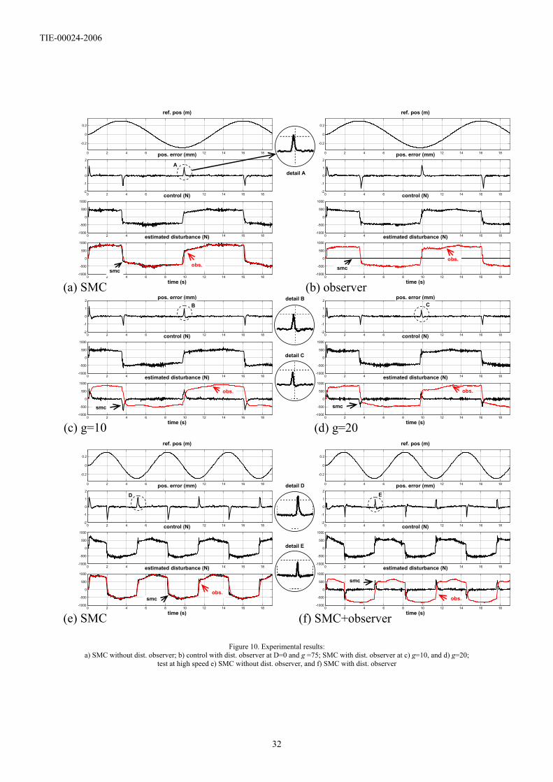
The experimental results are shown in Fig.10. Firstly, the disturbance estimation performance was
tested by comparison between the control by the pure SMC algorithm (21) and the control with the
proposed observer (25) at D=0, i.e. the disturbance estimation by SMC was off. In the first case, the system
disturbance observer was also implemented, but not connected in the loop. The results are shown by
Fig.10-a and Fig.10-b, respectively. In Fig.10-a the disturbance estimation signals are practically
overlapped. However, the observer dynamics was actually slower though g=D=75. Consequently, higher
position error peaks appeared as shown in Fig.10-b (here g=75, D=0). The position error peaks appeared at
the points of velocity reversals due to nonlinear friction effect. These results show that the pure SMC
algorithm performs better then control with the proposed disturbance observer.
Fig.10-c and Fig.10-d show results obtained by the proposed SMC with observer (25). Here, D=75
and the observer dynamics was set with g=10 and g=20 in Fig.10-c and Fig.10-d, respectively. Both, the
disturbance estimation by SMC and the proposed observer with slower dynamics were connected in the
control loop. As could be expected, the SMC estimated only the difference distτΔ , i.e. the portion which
the observer failed to output. It converged to zero value after the transient period. In comparison with the
results shown in Fig.10-a, position error peaks are lowered in both cases. Faster dynamics of the observer
caused lower position error, however, as noted by the theoretical analysis in Section III.E, only a
conservative disturbance observer dynamics could be set up in order to preserve stability of the system.

TIE-00024-2006
18
Larger values of the observer gain g caused oscillations in the system and ultimately led to instability.
Thus, the disturbance observer cut-off frequency was rather limited in the experiments.
Finally, experimental results at high reference speed are also presented. The results obtained by the
pure SMC algorithm are shown in Fig. 10-e (the disturbance observer is implemented but not connected in
the loop as in Fig.10-a), whereas Fig.10-f includes the results obtained by the proposed SMC with observer
at g=20. The diagrams show that the proposed control scheme extended by the system disturbance
observer lower position error peaks in amplitude and time duration both at low-speed and high speed
experiments.
V. CONCLUSION
The paper has proposed a new SMC control algorithm that is extended with the asymptotic
disturbance observer in order to improve position tracking performance at the points of velocity reversals,
where error peaks appear due to nonlinear friction characteristic. The disturbance observer has been
designed to estimate the system disturbance signal identified by the equivalent control that is not
measurable. It requires the reaction force signal for the realization, which is often not available in practice.
Thus, it should be estimated as proposed in this paper. It has been shown, that the compensation of the
reaction force is of significant importance for accuracy of the disturbance estimation, stability and
performance improvement of the closed-loop system. The estimated disturbance signal, which is perturbed
by the reaction force, can destabilize the system or only slow disturbance estimation dynamics can be
achieved. However, the experimental results have shown that even in the case of the erroneous model used
in the determination of the reaction force signal, improvement in the position error response has been
evident. The proposed scheme lower position error peaks in amplitude and time duration both at low-speed
and high speed experiments.

TIE-00024-2006
19
VI. ACKNOWLEDGEMENT
The authors gratefully acknowledge the contributions of ARRS-Slovenian Research Agency, and
Tübitak, The Scientific and Technical Research Council of Turkey, which partly financially supported the
joint research project "Sliding Modes in Motion Control Systems" of Institute of Robotics, University Of
Maribor, and Faculty of Engineering and Natural Science, Sabanci University, Istanbul-Turkey.

TIE-00024-2006
20
REFERENCES [1] M. Kagotani, T.Koyama, H. Ueda, "A study on transmission error in timing belt drives," ASME Journal of Mechanical
Design, Vol. 115, No. 12, pp. 1038-1043, 1993. [2] S. Abrate, “Vibration of belts and belt-drives,” Mechanism and machine theory, Vol. 27, No. 11, pp. 645-659, 1992. [3] Y. Hori, "Vibration suppression and disturbance rejection control on torsional systems," in Proc. of IFAC Workshop on
Motion Control, 1995, Munich, Germany , pp. 41-50. [4] I. Godler, M. Inoue, T. Ninomiya, T. Yamashita, "Robustness comparison of control schemes with disturbance
observers and with acceleration control loop," in Proc. of IEEE ISIE, 1999, Bled, Slovenia, pp.1035-1040. [5] P.B. Schmidt, R.D. Lorenz, "Design principles and implementation of acceleration feedback to improve performance of
DC drives," IEEE Trans. on Industry Applications, Vol. 28, No. 3, pp. 594-599, 1992. [6] K. Ohnishi, M. Shibata, T. Murakami, "Motion control for advanced mechatronics," IEEE/ASME Trans. on
Mechatronics, Vol. 1, No. 1, pp. 56-67, 1996. [7] H. Kawaharada, I. Godler, T. Ninomiya, H. Honda, "Vibration suppression control in 2-inertia system by using
estimated torsion torque," in Proc. of IEEE IECON, 2000, Nagoya-Japan, pp. 2219-2224. [8] K. Yuki, T. Murakami, K. Ohnishi, "Vibration control of 2 mass resonant system by resonance ratio control," in Proc.
of IEEE IECON, 1993, Vol. 3, pp. 2009-2014. [9] Y. Hori, H. Sawada, Y. Chun, "Slow resonance ratio control for vibration suppression and disturbance rejection in
torsional system," IEEE Trans. on Industrial Electronics, Vol. 46, No. 1, pp. 162-168, 1999. [10] M. Matsuoka, T. Murakami, K. Ohnishi, "Vibration Suppression and Disturbance Rejection Control of Flexible Link
Arm", in Proc. of the IECON, 1995, Vol. 2, pp. 1260-1265. [11] S. Katsura, J. Suzuki, K. Ohnishi, "Pushing Operation by Flexible Manipulator Taking Environmental Information into
Account," in Proc. of the AMC, 2004, Kawasaki, Japan, pp. 141-146. [12] R. Gorez, Y-L. Hsu, "Sliding mode control for displacements of servomechanisms with elastic joints," in Proc. of the
13th IFAC Triennial World Congress, 1996, San Francisco-USA, pp.43-48. [13] P. Korondi, H. Hashimoto, V. Utkin, "Direct torsion control of flexible shaft in an observer-based discrete-time sliding
mode," IEEE Trans. on Industrial Electronics, 1998, Vol. 45, No. 2, pp.291-296. [14] Y-F. Li, B. Eriksson, J. Wikander, "Sliding mode control of two-mass positioning systems," in Proc. of the 14th IFAC
Triennial World Congress, 1999, Beijing-China, pp.151-156. [15] V.I. Utkin, Sliding Modes in Control and Optimization. Springer-Verlag, Berlin, 1992. [16] A. Šabanović, K. Jezernik, K. Wada, “Chattering-free sliding modes in robotic manipulators control,“ Robotica, Vol.17,
No. 29., pp.17-29, 1996. [17] A. Hace, K. Jezernik, M. Terbuc, "Robust accurate motion control for belt-driven servomechanism," in Recent
Advances In Mechatronics, Kaynak, O., Editor. Springer-Verlag, Singapore, 1999. [18] A. Šabanović, Y. Yildiz, K. Abidi, N. Šabanović, "Sliding Mode Control of Timing-Belt Servo-system," in Proc. of
EDPE, 2003, The High Tatras, Slovak Republic, pp.55-60. [19] A. Hace, K. Jezernik, M. Terbuc, "VSS motion control for a laser cutting machine," Control Engineering Practice, Vol.
9, No. 1, pp. 67-77, 2001. [20] A. Hace, K. Jezernik, A. Šabanović, “Improved Design of VSS Controller for a Linear Belt-Driven Servomechanism,”
IEEE/ASME Transactions on Mechatronics, Vol. 10, No. 4, pp. 385-390, August 2005. [21] Y. Fujimoto, A. Kawamura, "Robust servo-system based on two-degree-of-freedom control with sliding mode," IEEE
Transactions on Industrial Electronics, Vol. 42, Issue 3, pp. 272 – 280, June 1995. [22] A. Šabanović, "Sliding Mode Framework in Motion Control. What it Offers?," in Proc. of AMC, 2004 March 25-28,
Kawasaki, Japan, pp.1-10. [23] B. Draženović, "The invariance conditions in variable structure systems," Automatica, Vol. 5, pp. 287-295, 1969.
TIE-00024-2006
21
LIST OF FIGURES
Figure 1. Vibrated response of a linear belt-drive Figure 2. Different control structures of a linear belt-drive: a) Cascaded control structure, b) Single loop
control structure, c) SMC with disturbance observer Figure 3. Linear belt-drive: a) Servomechanism, b) Spring model of the belt drive Figure 4. Block diagram of the belt-stretch model Figure 5. Closed-loop block diagram in sliding mode Figure 6. Chattering-free SMC with disturbance observer Figure 7. Proposed disturbance observer structure: a) Motor disturbance observer, b) Load disturbance
observer, c) System disturbance observer Figure 8. Experimental control system Figure 9. Typical response of the experimental linear drive: a) friction characterics, b) open-loop belt-
stretch response Figure 10. Experimental results: a) SMC without dist. observer; b) control with dist. observer at D=0 and
g =75; SMC with dist. observer at c) g=10, and d) g=20; test at high speed e) SMC without dist. observer, and f) SMC with dist. observer

TIE-00024-2006
22
LIST OF TABLES
Table I. Model parameters. Table II. Controller gains.

TIE-00024-2006
23
0 2 4 6 8 10 12 14 16 18 20
-0.2
0
0.2
POSITION (m)
0 2 4 6 8 10 12 14 16 18 20-0.5
0
0.5SPEED (m/s)
0 2 4 6 8 10 12 14 16 18 20
-2
0
2
ERROR (mm)error (mm)
ref. position (m)
velocity (m/s)
Figure 1. Vibrated response of a linear belt-drive

TIE-00024-2006
24
a)
b)
Belt-Drive position tracking
vibration-free SMC
-
belt-stretch
act. pos.
ref. pos.
Belt-Drive Vibration controller
position tracking SMC
Vibration-free control plant-
belt-stretch
act. pos.
ref. pos.
c)
Belt-Drive position tracking
vibration-free SMC
-
belt-stretch
act. pos.
ref. pos.
Dist. Observer
Figure 2. Different control structures of a linear belt-drive: a) Cascaded control structure, b) Single loop control structure, c) SMC with disturbance observer

TIE-00024-2006
25
x
R R
speed reducer
cart
G,
motor
ϕ, τ
Jm
J1 J2
Mc
JG
pulley
belt
carriage
a)
x
Mc
J1 q1
RJ2
q2
R
K2K1
K3
b)
Figure 3. Linear belt-drive: a) Servomechanism, b) Spring model of the belt drive

TIE-00024-2006
26
τwf τ
ff
1/p1/pK1/p1/p
Kw
belt-stretch dynamicsload-side dynamics
w w w x x x1/M-
1/J -
-
Figure 4. Block diagram of the belt-stretch model

TIE-00024-2006
27
ca x-
xx
- 1p
( )r t 1p( )wH p
vK
pK
Figure 5. Closed-loop block diagram in sliding mode

TIE-00024-2006
28
( )r t τσ eqτSMCτSMCτ
-
znominalplant
-
distτ
1p
0Dσ σ+ =
G
equiv. control belt-drive
dist. observer
ˆdistτ
position tracking vibration-free
SMC
Figure 6. Chattering-free SMC with disturbance observer

TIE-00024-2006
29
ˆreacτ
ϕϕ 1Jp
-
distτ
1p
gJ
gp g+
gJ
+
+ +
-+
ˆdistτ
reacτ +
+
-
τ
motor disturbance
observer
a)
xx1Mp
-
distf
1p
gM
gp g+
+
+ +
-+
ˆ distf
reacf
load disturbance
observer gM
ˆ reacf
b)
z nominal plant
-
distτ belt-drive
SMCτ τ eqτ
ˆdistτ
x
ϕ
w
reacf
reacτ-
motor dist.observer
load dist.observer
reac. forceestimator
ζ
+
ˆfτ ˆ
ff
disturbanceobserver
c)
Figure 7. Proposed disturbance observer structure: a) Motor disturbance observer, b) Load disturbance observer, c) System disturbance observer

TIE-00024-2006
30
current command
TCP/IPMatlab / Simulink
& Real-Time Workshop
WINDOWS XP
developing & monitoring
station
I/O
boa
rd
QNX Neutrino
controller Ts = 2ms
Intel Celeron 333MHz
motor angle
carriage position
RT-LAB
linea
r be
lt-dr
ive
Figure 8. Experimental control system

TIE-00024-2006
31
-0.4 -0.3 -0.2 -0.1 0 0.1 0.2 0.3 0.4-500
-400
-300
-200
-100
0
100
200
300
400
500
speed (m/s)
frict
ion
(N)
a)
0 0.5 1 1.5 2 2.5 3 3.5 4 4.5 5 -0.6
-0.4
-0.2
0.0
0.2
0.4
0.6
0.8
1.0
time (s)
w (m
m)
b)
Figure 9. Typical response of the experimental linear drive: a) friction characterics, b) open-loop belt-stretch response
TIE-00024-2006
32
0 2 4 6 8 10 12 14 16 18
-0.2
0
0.2
POSITION (m)
0 2 4 6 8 10 12 14 16 18-2
-1
0
1
2ERROR (mm)
0 2 4 6 8 10 12 14 16 18-1000
-500
0
500
1000CONTROL (N)
0 2 4 6 8 10 12 14 16 18-1000
-500
0
500
1000DISTURBANCE (N)
time (s)
0 2 4 6 8 10 12 14 16 18
-0.2
0
0.2
POSITION (m)
0 2 4 6 8 10 12 14 16 18-2
-1
0
1
2ERROR (mm)
0 2 4 6 8 10 12 14 16 18-1000
-500
0
500
1000CONTROL (N)
0 2 4 6 8 10 12 14 16 18-1000
-500
0
500
1000DISTURBANCE (N)
time (s)time (s)
ref. pos (m)
pos. error (mm)
control (N)
estimated disturbance (N)
(a) SMC (b) observer time (s)
ref. pos (m)
pos. error (mm)
control (N)
estimated disturbance (N)
smc obs.
obs. smc
A detail A
0 2 4 6 8 10 12 14 16 18-2
-1
0
1
2ERROR (mm)
0 2 4 6 8 10 12 14 16 18-1000
-500
0
500
1000CONTROL (N)
0 2 4 6 8 10 12 14 16 18-1000
-500
0
500
1000DISTURBANCE (N)
time (s)
0 2 4 6 8 10 12 14 16 18-2
-1
0
1
2ERROR (mm)
0 2 4 6 8 10 12 14 16 18-1000
-500
0
500
1000CONTROL (N)
0 2 4 6 8 10 12 14 16 18-1000
-500
0
500
1000DISTURBANCE (N)
time (s)time (s)
pos. error (mm)
control (N)
estimated disturbance (N)
(c) g=10 (d) g=20 time (s)
pos. error (mm)
control (N)
estimated disturbance (N)
smc
obs. obs.
smc
B detail B
C
detail C
0 2 4 6 8 10 12 14 16 18
-0.2
0
0.2
POSITION (m)
0 2 4 6 8 10 12 14 16 18-2
-1
0
1
2ERROR (mm)
0 2 4 6 8 10 12 14 16 18-1000
-500
0
500
1000CONTROL (N)
0 2 4 6 8 10 12 14 16 18-1000
-500
0
500
1000DISTURBANCE (N)
time (s)
0 2 4 6 8 10 12 14 16 18
-0.2
0
0.2
POSITION (m)
0 2 4 6 8 10 12 14 16 18-2
-1
0
1
2ERROR (mm)
0 2 4 6 8 10 12 14 16 18-1000
-500
0
500
1000CONTROL (N)
0 2 4 6 8 10 12 14 16 18-1000
-500
0
500
1000DISTURBANCE (N)
time (s)time (s)
ref. pos (m)
pos. error (mm)
control (N)
estimated disturbance (N)
(e) SMC (f) SMC+observer time (s)
ref. pos (m)
pos. error (mm)
control (N)
estimated disturbance (N)
smc obs.
obs.
smc
D
detail D E
detail E
Figure 10. Experimental results:
a) SMC without dist. observer; b) control with dist. observer at D=0 and g =75; SMC with dist. observer at c) g=10, and d) g=20; test at high speed e) SMC without dist. observer, and f) SMC with dist. observer

TIE-00024-2006
33
TABLE I.MODEL PARAMETERS
Mm Ml ω0 K (kg) (kg) (rad/s) (N/m) 57 33 62.8 2.7e5
TABLE II. CONTROLLER GAINS
D α β Kv Kp 75 125.6 7888 50 625