smast contribution series #06-1101 an operational

29 November 2006 SMAST Contribution Series #06-1101- Brown et al. Operational Modeling: Part 2

SMAST Contribution Series #06-1101

An Operational Circulation Modeling System for the Gulf of Maine/Georges Bank Region, Part 2: Applications

Wendell S. Brown, Avijit Gangopadhyay, and Zhitao Yu School for Marine Science and Technology, University of Massachusetts Dartmouth,

706 South Rodney French Boulevard, New Bedford, MA 02744

[Submitted to the IEEE Journal of Oceanic Engineering - 7 June 2005]

ABSTRACT

This paper describes the implementation of a prototype operational system for providing near-real-time information on the ocean water property and circulation environment in the Gulf of Maine/Georges Bank region. This application of the Harvard Ocean Prediction System model was developed and tested during a 52-week sequence of weekly nowcast/forecasts. The initial single-SST-image assimilation format was expanded to a three-SST-image assimilation format to produce a more realistic thermocline. The model system was applied to the winter-like conditions of March 2002 and the summer conditions of August 2002, when the model temperature and velocity fields could be compared with moored time series measurements at several locations. The data assimilation AFMIS/HOPS model applications produced qualitatively correct ocean temperature and flow patterns. During late winter, the wind dominated the variability of the model ocean surface Ekman transport, Georges Bank north flank jet, and Maine Costal Current. During late summer, the assimilation of very warm SST dominated the variability of the model coastal upwelling, a stronger and more stable Georges Bank north flank jet, and Maine Coastal Current. The model did reveal a persistent anticyclone in the western central Gulf of Maine that has not been well documented. Quantitatively, the surface temperatures from the model converged with those measured by the Gulf of Maine Ocean Observing System (GoMOOS) within 4-6 days from the beginning of the model run. Further, while the variability of the model and observed temperatures generally tracked each other, there were cases in which differences between contemporary and climatological temperatures led to systematic offsets. The model/observed velocity comparisons, while in general not as good as those for temperature, did improve after 6-8 days and the assimilation of two SST images. Thus future work is needed to better understand the quantitative model/observation differences revealed by intercomparisons and to improve the initialization and assimilation protocols. 1. Introduction This paper is the second of a pair of papers describing the implementation of a prototype operational system for nowcasting and forecasting the ocean water property and circulation environment in the Gulf of Maine/Georges Bank region. Our work is motivated by a belief that significant advances can be made in fishery management if the daily to weekly (short-term) variability in the structures of ocean environmental and fish fields are known. With an eye toward producing this new type of management information, we have begun to construct an Advanced Fisheries Management Information System (AFMIS; Brown et al., 2001; Robinson et al., 2001), which features the combination of observations and models. When operational, AFMIS will provide short-term information on the variability of (a) ocean environment, (b) structure of important fish stocks and (c) even economic conditions. AFMIS will accomplish this in near real-time by integrating a coupled suite of models with a diversity of ocean- and fisheries-related data needed to operate the model components.

29 November 2006 SMAST Contribution Series #06-1101- Brown et al. Operational Modeling: Part 2 2

Brown et al. (2004) describe the initial AFMIS model system for the Gulf of Maine/Georges Bank region–the Harvard Ocean Prediction System (HOPS) data assimilation, physical circulation model. Therein, the development of the basic elements of the operational system, including the physical ocean model, the model initialization protocols, and the protocols for the assimilation of sea surface temperature (SST) were presented. In this paper, we focus on the results from a pair of two-week-long AFMIS/HOPS calculations during the late winter and summer 2002. In section 2 of this paper, we describe the setup of the AFMIS/HOPS model system. In section 3, we describe the operational protocol. In sections 4 and 5, respectively, we present the model results for a late winter period between 18 March and 18 April 2002 and for a typical summertime period during August 2002. The quality of the model results are compared with moored data available through the Gulf of Maine Ocean Observing System (GoMOOS). In section 6, we discuss the implications of the prototype operational AFMIS/HOPS results. 2. HOPS Physical Circulation Model The Harvard Ocean Prediction System is a flexible, portable and generic system for interdisciplinary nowcasting, forecasting and simulations. The heart of the system is a primitive equation (PE) physical dynamical model that is applicable to model domains ranging in depth from 10 to several thousand meters. HOPS is modular, thus facilitating its adaptation to specific applications. The accuracy of HOPS information is improved on-the-fly by assimilating available recent data in near-real-time. HOPS can assimilate several types of readily-available satellite data, including sea surface temperature (SST), color (SSC), and altimetry-measured height (SSH) data, as well as insitu data, using a variety of methods for data-assimilation, including a robust (sub-optimal) optimal interpolation (OI) scheme (Lozano et al., 1996) and a quasi-optimal scheme, error subspace statistical estimation (Lermusiaux, 2001). The HOPS circulation model employed here (Robinson et al., 2001) simulates the baroclinic dynamical response of the model ocean to surface meteorological forcing, subject to a set of constraints imposed at the boundaries. For this application, the model is run on the larger, lower-resolution (15 km) northwest Atlantic (NWA) domain into which is nested the smaller, higher-resolution (5 km) Gulf of Maine/Georges Bank region (GOM/GB) domain (see Figure 1). This configuration was adopted so that the important influence of Gulf Stream variability can be brought to bear on the GOM/GB domain variability (see Brown et al., 2004 for the details). However, an important component of GOM/GB circulation variability is due to the tides. Thus, while the HOPS does not simulate tidal dynamics explicitly, the model parameterizes tidal mixing effects in the GOM/GB domain. (The free surface HOPS model, presently being tested, does include tidal dynamics explicitly.) The model runs with 225s time steps on both domains. The HOPS model parameters for vertical mixing, tidal mixing, and the different open boundary conditions are presented in Table 1 for the NWA and GOM domains. The vertical mixing is Laplacian, with a fixed eddy viscosity of Av = 0.5 cm2 s-1 for both


domains. To allow for tidal mixing, the eddy diffusivity (Kv) for the higher-resolution GOM/GB domain is small (0.05 cm2 s-1) compared to that (0.5 cm2 s-1) for the lower-resolution NWA domain. Convective adjustment, which is applied when the water column is statically unstable, is parameterized with a vertical viscosity of Av

cvct and a vertical diffusivity of Kv

cvct, with the GOM/GB domain values being an order of magnitude larger than the NWA domain values. At the open boundaries, Orlanski radiation conditions (ORI; Orlanski, 1976) were applied for all variables. At the coast in both model domains, normal flows and tracer fluxes were set to zero. At coastal boundaries in the GOM/GB domain only, tangential flows are subjected to a “damped free-slip condition” or Rayleigh friction, with a relaxation time Tc = 1800s, a Gaussian decay horizontal-scale of 2 grid points, and Lc = 10 km. At the bottom, a dynamic stress balance is applied to the momentum equations, with a drag coefficient Cd = 2.5 x 10-3.

Figure 1. (left) The AFMIS/HOPS model domains: the lower-resolution (15km) Northwest Atlantic (NWA) model domain, in which is nested the higher-resolution (5km) Gulf of Maine/Georges Bank Region (GOM/GB) model domain. (Note: The smaller two domains were not used for this calculation.) (right) Location map of the GOM/GB region, emphasizing the National Data Buoy Center (NDBC) numbered ocean buoy sites and National Weather Service (NWS) coded coastal island station meteorological measurement sites. Horizontally, the parameterization of the subgrid-scale mixing processes and filtering of numerical noise is based on a Shapiro filter (Shapiro, 1970), whose parameters are order (p), number of applications per time step (q), and number of time steps per application (r). The Shapiro filter triad of values for p, q and r (the Fs in Table 1) were derived for each state variable (velocity U, V, and W; temperature t, salinity s, streamfunction Ψ, and vorticity ω) from (1) empirical relationships between effective diffusivity and horizontal scales, and (2) a compromise between smoothing computational noise and allowing physical instabilities (Lermusiaux, 1999).


3. Operational Ocean Forecasting The HOPS data-assimilation circulation model provides 4-D hindcasts, nowcasts and forecasts of water property and velocity fields. This section describes the results of the prototype operational application of the AFMIS/HOPS to winter and summer 2002 conditions in the Gulf of Maine/Georges Bank region. The details of the assimilation protocols appear in Brown et al. (2005). Table 1. The HOPS model parameters for operational runs in the NWA and GOM domains, respectively. Ld is the number of vertical levels from the bottom at which the friction is applied.

Mixing Parameters Northwest Atlantic Gulf of Maine

Vertical Mixing Coefficients Av= 0.5 cm2 s-1; Avcvct = 5.5 cm2 s-1

Kv= 0.5 cm2 s-1; Kvcvct = 5.5 cm2 s-1

Av= 0.5 cm2 s-1; Avcvct = 50 cm2 s-1

Kv= 0.05 cm2 s-1; Kvcvct = 50 cm2 s-1

Bottom Friction Ld = 1; Td = 756,000 s Ld = 1; Td = 756,000 s

Tidal Mixing Coefficient N/A 100 cm2 s-1

BC Parameters

Open Boundary Condition U,V,T,S,Ψ,ω: (ORI) U,V,T,S,Ψ,ω: (ORI)

Boundary Relaxation N/A See text

Data Assimilation See text

Shapiro Filter p,q and r

Values for Different

Variables

Fu,Fv: 4,1,1; Ft,Fs: 4,1,1

Fw: 2,2,1; Fψ: No

Fu,Fv: 4,1,1; Ft,Fs: 4,1,1

Fw: 2,5,1; Fψ: 2,1,1

On 15 June 2001, we began a year+ series of weekly prototype operational AFMIS model runs on the larger-scale NWA domain and the higher-resolution GOM/GB domain. During parts of that series, different wind forcing and data assimilation schemes were used as indicated in Figure 2. During the first five weeks, the Navy Fleet Numerical Meteorological and Oceanographic Center (FNMOC) “analysis” (i.e., nowcast and hindcast) winds and forecast winds were used to produce model wind stress forcing. Then we lost access to the FNMOC winds. During the following 12-week period, when we were implementing an alternate scheme for winds (see below), the model was run with no wind forcing. On week 18, we began forcing the model with nowcast wind stress derived from the National Data Buoy Center (NDBC) measured winds. The NDBC-derived nowcast wind stress fields were persisted for the model forecasts. From June through December 2001 (weeks 4-28), bottom temperature data from a cooperative bottom trawler survey were assimilated into the operational AFMIS/HOPS nowcast/forecasts at initialization (see Brown et al., 2004, for details).


With the beginning of SST assimilation in January 2002 (week 29; YD 07), the day that the model was run was shifted from Monday (MD 0) to Thursday (MD 3). In week 33 (YD 35) the FNMOC winds became available again, thus enabling more realistic forecasts. During the first four days of the week 33 model run (MD 0 – MD 3) through the Thursday nowcast, model wind stress forcing, derived from FNMOC analysis winds, was used. The following six days of model forecasts were forced by FNMOC-derived forecast wind stress. From week 33 (YD 35 – 4 Feb) through week 39 (YD 77), the weekly operational model runs consisted of FNMOC-derived wind stress forcing and the assimilation of a single mean Tuesday SST image. Starting in week 40 (YD84), the normal single SST image data assimilation protocol was replaced with a multi-run triple SST assimilation protocol. With this change, the normal warm start was replaced with a simple restart (i.e., “hot start”) of the week 39 Thursday nowcast and subsequently updated with two additional SST assimilations. The next section details this application. 4. Model Forecast Results: Winter 2002 (18 March – 4 April) The March-April 2002 late winter conditions were modeled with a trio of coupled model runs to produce a series of hindcasts, nowcasts and forecasts 18 March (YD 77) and 4 April 2002 (YD 94). The trio of separate, but linked, GOM/GB model runs (A, B and C) was begun on Thursday 21 March, with the normal warm start. The sequence of the model runs was forced by FNMOC-derived wind stress fields that were constructed from a linear interpolation of the 6-hourly FNMOC winds. A time series of an average of the NDBC-measured winds in the GOM/GB region (Figure 3a) emphasizes the energetic 2- to 4-day variability that is common for this time of year. The sequence of three SST images were assimilated into the model according to the Brown et al. (2004) protocols on the schedule indicated in Figure 3b.


Figure 2. Timeline of the AFMIS/HOPS model configurations for the weekly series of prototype operational nowcast/forecasts (green), starting in mid-June 2001 (YD 176). The color-coded bars indicate the weeks in which the model employed (1) bottom temperature assimilation (blue); (2) SST assimilation (yellow); (3) FNMOC wind forcing (red); and (4) NDBC wind forcing (black).

Figure 3a. A time series of domain-averaged NDBC wind stress during the study period.

| | | | | | |--------forecast-------|

SST Figure Refs. 6 7 A1 T-field Figure Refs 5 9a 9b 10 11

Figure 3b. The SST assimilation schedule during three linked model runs from 0000 UT 18 March through 0000 UT 4 April 2002. Model run A (computed on 21 March) was begun with a warm start (see text) preceding the YD 77 start time of the run. Model run B (computed on 25 March) was begun with a “hot start” of model run A at 0000 UT 22 March. Model run C (computed on 28 March) was begun with a hot start of run B at 0000 UT 25 March and proceeded to produce forecasts for 29 March through 3 April. The figure numbers of selected model results are indicated. 4.1 Model Run Descriptions On 21 March (YD 80), model run A was begun with a warm start using the 18 March (MD 0) FNMOC-derived wind stress field (see Figure 4) and a water property climatology as described in Brown et al. (2004). The warm start produced the MD 0 (YD 77) initial temperature and current fields shown in the Figure 5 transect. The initial model velocity field exhibits the general features of the Gulf of Maine non-tidal circulation, including a modest westward flow along the Maine coast and, though weak,


an eastward “jet” over the north flank of Georges Bank (i.e., north flank jet, or NFJ). The robust westward flow over most of Georges Bank at this time is consistent with the generally southwestward winds, which appear to be also retarding the usually stronger NFJ.

Figure 4. The FNMOC-derived surface wind stress field for 0000 UT 18 March 02 (YD 77; MD 0).

Figure 5. The initial temperature field (after warm start dynamic adjustments) for 0000 UT 18 March (YD 77; MD 0) along the cross-Gulf transect located in Figure 4. Isotachs (in cm/s) of the northeastward (white), zero (red), and southwestward (black) flows overlay the temperatures (in oC as color-coded to the right). The locations of GoMOOS Buoy E temperature sensors (dots) are shown near the Maine coast to the right.


Once initialized, the wind-forced model run A stepped forward in time, assimilating the YD 78 average SST field (Figure 6, left panel), according to the yellow schedule in Figure 3. Note that this SST image had limited influence on the evolving model fields because only those portions of the SST field with uncertainties less than 50% (about ½; see Figure 6) were assimilated (also see Brown et al., 2004). Run A was stopped at 0000 UT Friday 22 March (YD 81). Then, on 25 March (YD 84), model run B was begun with a simple restart of model run A and stepped forward, assimilating the acceptable portions of the YD 81-82 average SST field (Figure 7), according to the blue schedule (Figure 3). Because in this case most of the SST image was assimilated, it had a significant effect in evolving the model fields away from climatology and toward reality. Run B was stopped at 0000 UT 25 March (YD 84). Then on 28 March (YD 87), model run C was begun with a simple restart of model run B and stepped forward, assimilating the few acceptable portions of the YD 84-86 average SST field (see Appendix A, Figure A1) according to the red schedule in Figure 3.

Figure 6. (left) The full YD 77-79 average SST image. (right) The portions of the SST image, with uncertainties less than 50%, that were assimilated into run A. The temperature legend in oC is to the right.

4.2 Analysis of model results The importance of wind forcing for advection and mixing during this time of the year is demonstrated with some selected model temperature/current results from the study period. (The model results that we present occur about ½ day after an SST input (see Figure 3) so that the inevitable short term transients from the SST input could diminish significantly.) The cross-Gulf transects of temperature and current for YD 79 (MD 2; Figure 9a) and YD 84 (MD 7; Figure 9b) indicate an increased warming and thickening of the near-surface mixed layer in both the Gulf and over the Bank (relative to the YD 77 initial field; see Figure 5). This result is consistent with the combined warming indicated in the assimilated SST images and the mixing effects of the energetic surface winds. This particular episode of surface warming is the first of a sequence of vernal warming pulses that historically strengthen the stratification at 10-20 m. Figure 9b shows the beginnings of the surface layer of Maine Surface Water and the more persistent pool of Maine Intermediate Water (MIW) centered on a depth of 50 m.


Figure 7. (left) The full YD 81-82 average SST image. (right) The portions of the SST image, with uncertainties less than 50%, which were assimilated into run B. The temperature legend in oC is to the right.

The current fields also evolved significantly during the first 7 days of the combined model runs A and B. The north flank jet (NFJ), which was weak and submerged on YD 77 (MD 0) (see Figure 5), was stronger and nearly surfaced on YD 79 (MD 2), probably as a result of a diminished southwestward wind. The strong northeastward wind between YD 82 and 84 apparently caused the reversal of the general southwestward Maine Coastal Current. During several days leading up to 28 March (YD 87), a strong weather system with intensified northward winds moved northeastward through the GOM/GB region (see Figure 10a). These winds produced the strong, widespread, northeastward surface Ekman currents in the eastern Gulf on YD 87 (see Figure 10b & c). The bottom currents were very small (< 5 cm/s) throughout much of the Gulf and over the Bank at this time. Between 28 March (YD 87) and 3 April (YD 93), the forecast winds indicate that another major weather system was to traverse the region. However, by 0000 UTC 3 April (YD 93), the regional response was dominated by relatively light eastward wind forcing that induced weak southeastward model surface currents, particularly in the west. Still, the residual effects of the previous 2 days of northeastward winds remained, as evidence by an intensified northeastward Maine Coastal Current that fed a relatively strong outflow south of southwestern Nova Scotia. The model current transect (see Figure 11c) shows that the surface-to-bottom northeastward flow displaced the southwestward-flowing Maine Coastal Current offshore. At the same time, shelf/slope temperature front became vertical. The question of the accuracy of these model temperature and current fields is addressed next.


(a) YD 79 (MD 2)

(b) YD 84 (MD 7)

Figure 9. Temperatures and normal velocities along the cross-Gulf transect located in Figure 4 for: (a) Run A hindcast at MD 2 (YD 79; 20 March 2002); (b) Run B nowcast/Run C initialization (YD 84; 25 March 2002). Isotachs (in cm/s) of the northeastward (white), zero (red), and southwestward (black) flows overlay the temperatures (in oC as color-coded to the right). The locations of GoMOOS Buoy E temperature sensors (dots) are shown near the Maine coast to the right.


Figure 10a. Surface wind stress fields for the 28 March 2002 (YD 87) run C nowcast.

Figure 10b. Surface temperatures and current vectors for the 28 March 2002 (YD 87) run C nowcast.


Figure 10c. Temperatures and normal velocities along the cross-Gulf transect located in Figure 4 for the 28 March 2002 (YD 87) run C nowcast. Isotachs (in cm/s) of the northeastward (white), zero (red), and southwestward (black) flows overlay the temperatures (in oC as color-coded to the right). The locations of GoMOOS Buoy E temperature sensors (dots) are shown near the Maine coast to the right.


Figure11a. The surface wind stress field for the run C 6th-day forecast–3 April 2002 (YD 93).

Figure11b. The surface temperatures and current vectors.


Figure11c. Temperatures and normal velocities along the cross-Gulf transect located in Figure 4 for the 3 April 2002 (YD 93) run C nowcast. Isotachs (in cm/s) of the northeastward (white), zero (red), and southwestward (black) flows overlay the temperatures (in oC as color-coded to the right). The locations of GoMOOS Buoy E temperature sensors (dots) are shown near the Maine coast to the right.

4.3 Model Quality Assessment – Model/Observation Comparisons The quality of these model results is evaluated in terms of time series comparisons with available buoy measurements (see Figure 12). Specifically, model temperature time series (Figure 13) were compared with Gulf of Maine Ocean Observation System (GoMOOS) and National Data Buoy Center buoy temperature records at 1m depths. For ocean velocities, depth-averaged GoMOOS and model velocities were compared at two locations. The temperature and velocity time series were low-pass filtered to remove tidal frequency variability that is not produced in the AFMIS/HOPS circulation model results. To minimize the model/observation differences due to differences between the real and model local bathymetry, we averaged the model time series at nine model grid locations (covering approximately 10 km2) surrounding each buoy location (see Figure 12 inset). The time/space-smoothed, near-surface (1m-depth) model temperature time series are compared with the corresponding measurements from (a) two GoMOOS buoys (I and E) from coastal Maine and (b) NDBC buoys in the central Gulf (44008) and on Georges Bank (44005; see Figures 1 and 12). Comparisons in Figure 13 generally show that the initial model temperatures were systematically cooler than the buoy temperatures,


indicating that March 2002 was warmer than climatology. (The climatology is an average of the March temperature hydrography from the previous 20 years). The Figure 13 comparisons show that the SST-assimilation process warms the model ocean enough so that the temperatures converge with the four buoy-measured near-surface temperatures (within the uncertainty of the assimilated SST). Starting on 22 March, the GoMOOS Buoy-E-measured temperature decreased rapidly from about 4.8oC to 3.9oC. Encouragingly, the latter is consistent with the relevant SST near-surface temperatures in the region (see Table 2). The model temperature at Buoy E tracks this decrease in Buoy E temperature and the rest of the record reasonably well. The tracking of model and buoy near-surface temperatures at the other sites is reasonable except at NDBC 44008 on Georges Bank, where behaviors are distinctly different for unexplained reasons.

Figure 12. Locations of the GoMOOS and NDBC buoys used in the model/data comparisons. The model results from the nine grid locations (red dots) surrounding each respective buoy location (blue dot) are averaged.

Table 2. The mean SST temperature at the location of GoMOOS Buoy E (see Figure 12 for location). Date 2002 Year Day

19/18 March 78/77

23/21 March 82/80

26/25 March 85/84

Temperature (oC) 4.98 4.50 4.50


(a) (b)

(c) (d)

Figure13. Model near-surface (1m-depth) temperature time series: hourly (red); tide-filtered (green). Tide-filtered near-surface buoy-measured temperatures (black) at (a) GoMOOS Buoy E and (b) GoMOOS Buoy I and at (c) NDBC Buoy 44005 and (d) NDBC Buoy 44008. Blue lines indicate the uncertainty limits for the three different SST images that were assimilated into the model run.

Given the SST assimilation, it is reassuring that the model near-surface temperature tracks the assimilation SST temperature very well. A sterner test is the model/observation comparison of the deeper temperatures as shown in Figure 14, and the results are more mixed. For example, even after the initial adjustment period, the model temperatures at Buoy E at 20m (and 50m) depth (Figure 14) fail to converge with the observed temperatures. The good news is that the model temperatures track the variability in the observed temperatures quite well. The bad news is that the 20m model temperatures remain systematically offset by about 1oC from the GoMOOS Buoy E temperatures. While reducing the climatology/March 2002 environmental temperature difference of about 1-2oC, the SST assimilation process was not robust enough to complete the convergence. Why the offset persists, despite record variabilities that track quite well, is unknown. At 50 m, the initial model (i.e., climatological) and measured ocean temperatures were very similar at the start and remained so for the duration. Overall, however, the model-versus-buoy temperature measurement comparisons were encouragingly reasonable.


The comparisons between the model and GoMOOS buoy depth-averaged velocities in Figure 15 show improved correspondence after the approximately 7 days of run time and 2 SST assimilations. (The corresponding temperature comparisons showed dramatic convergence after about 4 days and 1 SST assimilation.) Despite some similarity, the model velocities have much less variance than the observed velocities. In particular, while the weekly fluctuations in the observed velocities are approximately simulated by the model, the 3-5 day velocity fluctuations are not. Given the energetic 2-5 day variability in the wind forcing, it is difficult to explain the lack of model velocity energy in that frequency band. Clearly, a more in-depth diagnosis of the model velocity field variability is needed.

GoMOOS Buoy E

(a) 20m (b) 50m

GoMOOS Buoy I

(c) 20m (d) 50m Figure 14. Model temperature time series: hourly (red); tide-filtered (green). Tide-filtered buoy-measured temperatures (black) at GoMOOS Buoy E at (a) 20 m and (b) 50 m, and at GoMOOS Buoy I at (c) 20 m and (d) 50 m.


Figure 15. Velocity component time-series comparison between the forecast (red) and data (blue). The top panels are for Buoy I and the bottom panels are for Buoy E. The eastward components are shown on the left, and the northward components are on the right.

4.4 Model Forecast Skill: Winter 2002 Temperatures The forecast skill of these model results is presented in terms of the model forecast bias (BIAS; the time average of the difference between the observation and the forecast), mean error (ME), mean absolute error (MAE), root mean square error (RMS), and maximum error (MAX). (See Appendix B for definitions.) Generally speaking however, smaller bias and rms errors indicate better prediction skill. The model temperature forecast skills were computed for time series results between 29 March and 4 April at GoMOOS Buoys E and I and NDBC Buoys 44005 and 44008 (see Figures 13 and 14). At Buoy E, the model forecast temperature bias at 1m depth is 0.08˚C (see Table 3), increasing with depth. However, the corresponding model temperature rms and the maximum errors decrease with depth. At Buoy I, the model forecast temperature bias varies from zero at 1m to about -0.10 ˚C at 50m depth. The corresponding model temperature rms and the maximum errors vary little throughout the water column. The model forecast surface temperature biases at the 2 NDBC buoy sites are about ±0.4 ˚C, substantially greater than those at the GoMOOS buoy sites. The NDBC buoy sensors may not be as accurate as the GoMOOS buoy sensors. We intend to explore these issues soon.


The relatively larger model forecast surface temperature bias at GoMOOS buoy E suggests that there is room for improvement in the way that we initialize model calculations. We will be exploring new ways to implement a FORMS feature-oriented model calibration. Other errors may be introduced by using FNMOC winds to estimate the mixed layer depth in our SST assimilation. We intend to explore using real NDBC winds instead of FNMOC model-derived winds to improve forecast skills.

Table 3. Model temperature forecast skill for the March 2002 study.

WINTER SUMMER

DEPTH STATS Buoy E Buoy I NDBC 44005

NDBC 44008

Buoy E Buoy I

BIAS 0.08 0.00 0.38 -0.47 -0.40 -1.04 MAE 0.18 0.07 0.09 0.19 0.52 0.34 RMS 0.21 0.08 0.11 0.23 0.63 0.43

1 m

MAX 0.50 0.14 0.23 0.49 1.23 0.68 BIAS 1.01 -0.11 -0.84 -1.07 MAE 0.06 0.06 0.08 0.21 RMS 0.06 0.07 0.09 0.26

20 m

MAX 0.12 0.16 0.19 0.57 BIAS 1.62 -0.09 0.58 1.19 MAE 0.04 0.03 0.05 0.06 RMS 0.05 0.04 0.05 0.08

50 m

MAX 0.09 0.08 0.09 0.25

5. Model Forecast Results: August 2002 The August 2002 summer conditions were modeled with a single model run on 15 August 2002 (YD 220) that produced hindcast, nowcast and forecast results between 0000 UT, Monday, 5 August (YD 217) and 0000 UT, Thursday, 22 August (YD 234). The model (1) was forced by the appropriate analysis and forecast FNMOC-derived wind stress fields with a domain-average variability depicted in Figure 16a, and (2) assimilated three separate SST average images (YD 217-YD 219; YD 217-YD 223; and YD 224-YD 226) on the schedules presented in Figure 16b. During this summer study period, the winds were light, so that the predominant model ocean evolution was forced by the assimilation SST fields, which were much warmer than the climatology used for the model warm start. The evolution of the model temperature and velocity fields over the study period is depicted in the following suite of horizontal and vertical sections. The effect of the warm start on the pre-warm-start (i.e., unadjusted) initial ocean surface temperature field is shown in the pair of Figure 17 transects. The warm-start-induced dynamic adjustments cause the shelf/slope front on the southern flank of Georges Bank to move a little to the north relative to the climatologically dominated initial field (see Figure 17b). In this adjusted field, Georges Bank is cooler, and a more well-developed tidal front appears on the north flank of Bank. The prescribed model tidal mixing atop the Bank in HOPS is the probable cause of this development. The impact of SST assimilation shows first as some “hot spots” on the upper ocean (just like the winter case).


Figure 16a. A time series of domain-averaged NDBC wind stress during the study period.

|------forecast------| | | | | | | Fig, Refs 17a 17b 19a 19b Figure 16b. A real-time AFMIS/HOPS circulation model run on 15 August 2002 assimilated three different mean SST fields according to the indicated weighting structure. The warm-start initialization of the model run is referenced to 0000 UT 5 August 2002 (YD 217). The initial model hindcast temperature field for Monday, 5 August 2002 (YD 217) is defined by intermediate-warmth, well-mixed Georges Bank water that transitions to cooler Gulf of Maine Surface Water (SW), cold Maine Intermediate Water (MIW) from 50 to 150 meters, and slightly warmer Maine Bottom Water (MBW) in Wilkinson Basin. The NFJ and Maine Coastal Current are prominent. In this dynamically balanced initial field, there is a broad flow on the southern flank of Georges Bank going southwestward along a nearly vertical shelf/slope front.


.

(a) MD -2

(b) YD 217

Figure 17. The pre- and post-warm-start model temperature field transects (located in Figure 4): (a) pre-warm-start initial field (MD –2); (b) post-warm start, dynamically adjusted hindcast temperature and normal velocity fields for 5 August 2002 (YD 217). Isotachs (in cm/s) of the northeastward (white), zero (red), and southwestward (black) flows overlay the temperatures (in oC as color-coded to the right). The locations of GoMOOS Buoy E temperature sensors (dots) are shown near the Maine coast to the right.

However the initial model SST (YD 217) pattern has the smoothed look of the climatology from which it was derived. It then is rapidly changed by the assimilation of the YD 218 average SST field (Figure 18b). Subsequent SST assimilations (see


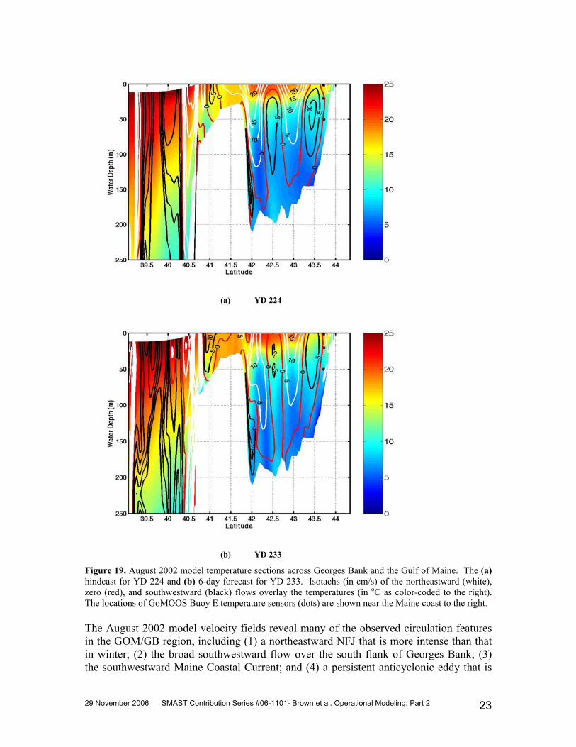
Appendix A) combined with FNMOC-derived wind forcing help to evolve the model fields further, leading to the 3-day forecast SST field on YD 230 (Figure 18c). The contrast between the initial model surface temperature fields (Figures 17 & 18a) and the forecast model surface temperature results for 18 August (YD 230; Figures 18c) is consistent with the strong thermal forcing of the near-surface layer in the time interval. (Note: The wind stresses were generally from the southwest during this time and not strong enough to significantly modify the basic baroclinic circulation pattern in the Gulf of Maine.) Temperatures in the upper 20-30 m of the Gulf of Maine are forced (through assimilation) to increase from about 15oC in the YD 217 initial field to about 20oC by the YD 224 hindcast and to about 23oC by the 6-day (YD 233) forecast (Figure 19). Further, warming of the upper layer of the Gulf and atop Georges Bank (plus some modest wind-forcing) causes the deepening of the upper layer and other changes. The HOPS tidal mixing induces a warming of the whole water column of Georges Bank.

(a) model SST YD 217 (b) YD 218 Average SST

(c) YD 230 (d) Figure 18. (a) The model hindcast surface temperature field for 5 August 2002 (YD 217). (b) The YD 217-YD 219 average SST image was the first of three images that were assimilated into the model according to the Figure 16b schedule. (c) The model forecast surface temperature and (d) bottom temperature fields for 18 August 2002 (YD 230). The temperature (oC) legend is shown to the right.


(a) YD 224

(b) YD 233

Figure 19. August 2002 model temperature sections across Georges Bank and the Gulf of Maine. The (a) hindcast for YD 224 and (b) 6-day forecast for YD 233. Isotachs (in cm/s) of the northeastward (white), zero (red), and southwestward (black) flows overlay the temperatures (in oC as color-coded to the right). The locations of GoMOOS Buoy E temperature sensors (dots) are shown near the Maine coast to the right. The August 2002 model velocity fields reveal many of the observed circulation features in the GOM/GB region, including (1) a northeastward NFJ that is more intense than that in winter; (2) the broad southwestward flow over the south flank of Georges Bank; (3) the southwestward Maine Coastal Current; and (4) a persistent anticyclonic eddy that is


centered on the sill between Georges and Wilkinson Basins. The latter feature is less well-documented observationally and deserves more attention. The fidelity of the comparisons of the model temperature time-series at GoMOOS Buoys E and I (see Figure 20) are comparable to those from March. The model temperature forecast skills were calculated for the 16 through 21 August period at the sites of GoMOOS Buoys E and I. At Buoy E, the forecast 1m temperature bias is -0.40˚C, and at Buoy I the bias is -1.04˚C (see Table 3)–both greater than the corresponding biases in March. We do not present a comparison of August 2002 model versus observed velocity variations, because their temporal variations were very slow with low amplitude. Thus the statistical skill results were not statistically significant.

(a) (b) Figure 20. Comparisons of model temperature (red, green) versus GoMOOS buoy temperatures (black) at depths of 1 m, 20 m and 50 m for 5-22 August 2002 at (a) buoy E and (b) buoy I. Blue lines indicate the uncertainties for the three different SST images that were assimilated into the model run. The dashed lines indicate loss of buoy data. 6. Discussion and Summary In this paper, we describe the application of our AFMIS/HOPS operational modeling system to the Gulf of Maine/Georges Bank region for a typical late winter scenario in March 2002 and a late summer scenario in August 2002. These very similar applications evolved out of a year+ of weekly model nowcast/forecast runs that involved FNMOC-derived wind stress forcing and the assimilation of a single average SST image. These winter and summer applications employed an expanded 2-week model calculation protocol, in which three separate SST images were assimilated so that the thermocline could develop more realistically. In the March-April 2002 study, three separate model runs were coupled to allow the hindcast model fields to first develop fully over the first week and then transition into a forecast mode during the second week. In the August 2002 study, a single model calculation, involving three separate SST assimilations,


provided a week and a half of hindcast model results leading up to the nowcast fields and followed by 6 days of forecast fields. The data assimilation AFMIS/HOPS model applications produced qualitatively correct ocean temperature and flow patterns. During late winter, the ocean gradually warmed, but the wind dominated the model ocean variability, which featured surface Ekman transport and highly variable Georges Bank north flank jet and Maine Costal Current. During late summer, with relatively weak winds, the assimilation of very warm SST dominated the model ocean variability, which featured some coastal upwelling, and stronger and more stable Georges Bank north flank jet and Maine Coastal Current. The model did reveal a persistent anticyclone in the western center of the the Gulf of Maine that has not been well documented. Quantitatively, the surface temperatures from the model converged with those measured by the Gulf of Maine Ocean Observing System (GoMOOS) within 4-6 days from the beginning of the model run. Further, while the variability of the model and observed temperatures tracked each other in general, in some cases there were offsets due to differences between contemporary and climatological temperatures. The model/observed velocity comparisons, while in general not as good as those for temperature, did improve after 6-8 days and assimilation of two SST images. The validation studies, involving comparisons of model results with GoMOOS data, generally show the convergence of model and buoy-measured surface temperatures within 4-7 days, with deeper temperatures taking a few days longer. Still, in some cases at depth, the model/observation temperatures did not converge, although the shorter term variabilities may have tracked each other. There were systematic temperature differences at depth, probably as a result of either inadequate SST-assimilation protocols or the Mellor-Yamada (1982) vertical mixing schemes or both. These differences point toward the need for: (i) calibration of synoptic feature models with observed SST to improve the vertical profile at initialization, (ii) assimilation of available GoMOOS buoy data at nowcast and forecast times, (iii) addition of heat flux in the forecast mode, (iv) recalculation of mixed-layer depth for SST assimilation with forecast wind fields, and/or (v) using assimilating buoy data at critical locations.

The goal of the work described here was to develop a physical circulation model forecast system for the Gulf of Maine that would provide real-time, fine-scale hindcast, nowcast and forecast information about the three-dimensional physical ocean environment. The quality assessment of the model results indicates reasonable success in nowcasting and short-term forecasting of the temperature fields. The assmilation of satellite SST was clearly helpful in this regard. The less-satisfying quality of the model velocities is probably in part due to the lack of explicit tidal variability in the HOPS model used in a highly nonlinear regime of GOM/GB tides. Thus in the near future we will be looking to adapt this methodology to a circulation model with a free surface. Reasonable candidates include the Dartmouth finite element model QUODDY (Lynch et al., 1996; 1997), the Princeton Ocean Model or perhaps the newer Chen Finite-Volume Coastal Ocean Model (FVCOM). Once the velocity nowcasting/forecasting skills are improved sufficiently, we can begin developing model protocols to nowcast/forecast fish or at fish larvae fields.

7. Appendices

Appendix A: SST Assimilation Fields The third SST image assimilated into the March 2002 model run C demonstrates how cloudiness can degrade the usefulness of such images at times. In this case, only about 25% of the surface temperature information – and that around the periphery of the domain – was useful.


Figure A1. (left) The full SST image for YD 85 SST (i.e., YD 84-86 average) assimilation into run C. (right) The portions of the image that have uncertainties less than 50%. The temperature legend in oC is to the right. The second and third SST images (Figures A2 and A3) assimilated into the August 2002 model run were similarly warm and, like the first SST image in the trio, had negligible observational errors (see Brown et al., 2004), particularly compared to the first and third March images (Figure A1).

Figure A2. (left) The YD 217-YD 223 average SST image. (right) Observation errors associated with the corresponding SST image.

Figure A3. (left) The YD 224-YD 226 average SST image. (right) Observation errors associated with the

corresponding SST image.


Appendix B: Model Skill Algorithms The model forecasts are imperfect estimates of the true state of the ocean. It is of critical importance to understand the range and distribution of model errors. We conducted a skill analysis of the model forecasts described in the main text. GoMOOS buoy measurements were used as the standard for evaluating the fidelity of the model forecasts. We first calculated the model forecast/observation bias, defined by Vested et al. (1995) as:

FRCOBSBIAS −= , (1) where the bracket represents an average over all point-by-point differences between observation (OBS) and the model forecast (FRC) at the observation station. Then we computed the mean error (ME), mean absolute error (MAE), root mean square error (RMS), and maximum error (MAX), which were all functions of the forecast range (RES), where CFROBSRES ′−= is the difference between the observation and the bias-corrected forecast BIASFRCCFR +=′ at the observing station, according to the following:

∑=

=N

niRES

NME

1

1 (2)

∑=

=N

niRES

NMAE

1

1 (3)

( )∑=

−=N

ni MERES

NRMS

1

21 (4)

( ) ( )( )NRESABSRESABSMAX ,,max 1 K= (5)

8. Acknowledgments This work has benefited from the major effort by A.R. Robinson (Harvard), his modeling group and former SMAST personnel in developing the technology that has been used for this application. Harvard’s C. Lozano and P. Haley and SMAST’s H.-S. Kim and L. Lanerolle contributed in important ways to the implementation of the RFAC AFMIS. This research was funded by the National Aeronautics and Space Administration under a number of grants, including NAG 13-48 and, most recently, NAG5-9752.

9. References Brown, W.S., Bub, F.L., Rothschild, B., Sundermeyer, M., Gangopadhyay, A., Lane, R.,

Robinson, A.R., and Haley, P., 2001. Assimilating near-real-time fisheries and environmental data into an advanced fisheries management information system.


Paper presented at the 2001 ICES Annual Science Conference, Oslo, Norway, 25-29 September.

Brown, W.S., Gangopadhyay, A., Bub, F.L., Yu, Z., Strout, G., and Robinson, A.R.,

2005. An operational modeling system for the Gulf of Maine/Georges Bank region, part 1: Basic elements. University of Massachusetts Dartmouth, School for Marine Science and Technology, New Bedford, MA 02744, SMAST Contribution Series #06-1001.

Chao, Y., Li, Z., Kindle, J., Paduan, J., and Chavez, F., 2003. A high-resolution surface

vector wind product for coastal oceans: blending satellite scatterometer measurements with regional mesoscale atmospheric model simulations. Geophys. Res. Lett., 30(1), 1013.

Chen, C., Liu, H., and Beardsley, R.C., 2002. An unstructured, finite-volume, three-

dimensional, primitive equation ocean model: application to coastal ocean and estuaries. J. Atmos. Ocean. Tech., 20:159-186.

Lermusiaux, P.F.J., 1999. Estimation and study of mesoscale variability in the Strait of

Sicily. Dyn. Atmos. Oceans, 29, 255-303. Lermusiaux, P.F.J., 2001. Evolving the subspace of the three-dimensional multiscale

ocean variability: Massachusetts Bay. J. Marine Syst., 29 (1-4):385-422. Lozano, C.J., Robinson, A.R., Arango, H.G., Gangopadhyay, A., Sloan, N.Q., Haley,

P.J., and Leslie, W.G., 1996. An Interdisciplinary Ocean Prediction System: Assimilation Strategies and Structured Data Models. In: P. Malanotte-Rizzoli (Editor), Modern Approaches to Data Assimilation in Ocean Modelling, Elsevier Oceanography Series, Elsevier, Amsterdam, pp. 413–452.

Lynch, D.R., J.T.C. Ip, C.E. Naimie, and F.E. Werner, 1996. Comprehensive coastal

circulation model with application to the Gulf of Maine. Cont. Shelf Res., 16, 875-906.

Lynch, D.R., M.J. Holboke, and C.E. Naimie, 1997. The Maine coastal current: Spring

climatological circulation. Cont. Shelf Res., 17, 605-636. Mellor, G.L., and Yamada, T., 1982. Development of a turbulence closure model for

geophysical fluid problems. Rev. Geophys. Space Phys., 20, 851-875. Orlanski, I., 1976. A simple boundary condition for unbounded hyperbolic flows. J.

Comput. Phys., 21, 251-269. Robinson, A.R., Rothschild, B.J., Leslie, W.G., Bisagni, J.J., Borges, M.F., Brown, W.S.,

Cai, D., Fortier, P., Gangopadhyay, A., Haley, P.J. Jr., Kim, H.S., Lanerolle, L., Lermusiaux, P.F.J., Lozano, C.J., Miller, M.G., Strout, G., and Sundermeyer, M.A., 2001. The development and demonstration of an Advanced Fisheries


Management Information System (AFMIS). Invited paper presented at the January 2001meeting of the Amer. Meteorol. Soc., Albuquerque, NM, 186-190.

Shapiro, R., 1970. Smoothing, filtering, and boundary effects. Rev. Geophys. Space

Phys., 8: 359-387. Vested, H. J., J. W. Nielsen, H. R. Jensen, and K. B. Kristensen, 1995. Skill assessment

of an operational hydrodynamic forecast system for the North Sea and Danish Belts. In Quantitative Skill Assessment for Coastal Ocean Models, D. R. Lynch and A. M. Davis Eds. American Geophysical Union, 373-396.

smast contribution series #06-1101 an operational

Documents