smart system of renewable energy storage based on ... · invade h2020 project ... flexibility from...
TRANSCRIPT

INVADE H2020 project – Grant agreement nº. 731148
This project has received funding from the European Union’s Horizon 2020
Research and Innovation programme under Grant Agreement No 731148.
Smart system of renewable energy storage based on INtegrated EVs and
bAtteries to empower mobile, Distributed and centralised Energy storage
in the distribution grid
Deliverable nº: D5.3
Deliverable name: Simplified Battery operation and control algorithm
Version: 1.0
Release date: 20/12/2017
Dissemination level: Public (Public, Confidential)
Status: Submitted (Draft, Peer-reviewed, Submitted, Approved)
Author: Stig Ødegaard Ottesen – eSmart
Pol Olivella-Rosell, Pau Lloret – UPC
Ari Hentunen - VTT
Pedro Crespo del Granado, Sigurd Bjarghov, Venkatachalam Lakshmanan, Jamshid Aghaei, Magnus Korpås and Hossein Farahmand – NTNU

INVADE H2020 project – Grant agreement nº. 731148
D5.3 Simplified Battery operation and control algorithm Page 2 of 4
Document history
Version Date of issue Content and changes Edited by
0.1 30/11/2017 Executive summary H. Farahmand and V.
Lakshmanan
0.2 05/12/2017 Final editing P. Crespo del Granado
1.0 20/12/2018 Revision H. Farahmand and V.
Lakshmanan
Peer reviewed by:
Partner Reviewer
SIN Jayaprakash Rajasekharan
GreenFlux Michel Bayings
Deliverable beneficiaries:
WP / Task
WP5 / Task 5.3 and 5.4
WP8 / Task T8.3
WP10
INVADE H2020 project – Grant agreement nº. 731148
D5.3 Simplified Battery operation and control algorithm Page 3 of 4
Executive summary
The main objective of the INVADE project is to study possibilities to increase RES
penetration and integration in the power system by adding more storage, i.e., batteries.
The analysis centres on the flexibility services that different types of storages can
provide, namely: centralized, distributed and mobile (EVs). The focus of the work
package 5 (WP5) is to assess flexibility and perform analysis in order to investigate the
optimal deployment of flexibility sources. Solutions to reduce the challenges brought by
variable RES and EV charging include both the added flexibility on the supply and load
side. Combining the different characteristics of these resources is essential in assessing
the value of distributed energy resources in the power system and in the energy market.
The main objective of this WP is to study how to achieve optimal deployment of flexible
energy storage in distribution systems. This would lead to an improved use of existing
power system infrastructure and reduce issues caused by variable renewable energy
sources in the physical electricity systems and at the electricity markets.
Deliverable D5.3 provides a simple model for flexibility operation and planning to serve
distribution system operators (DSO), balance responsible parties (BRPs) and
Prosumers. This is a simplified model that will be initially implemented in the INVADE
Platform. This report contains the first version of flexibility management allocation and
operation algorithms. The focus is to develop an optimisation method for the operation
of stationary and EV batteries as energy storage assets in the distribution grid. The
motivation is that storage applications could help to improve the flexibility of the demand
side, which again enables a more efficient integration of supply from renewable energy
sources. To cope with the intermittent output of RES production, the
charging/discharging scheduling of battery storage systems will be carried out with
respect to the load and supply variations. The reaction of batteries to net-load variation
provides a fast response to imbalances in the system before other frequency control
activation. This can effectively help the frequency quality of a RES dominated power
system. Moreover, we include the optimal siting and sizing of batteries from the use case,
application and grid operation point of view. This is important to ensure that the batteries
can effectively contribute to the network management and mitigation of operating
challenges.

INVADE H2020 project – Grant agreement nº. 731148
D5.3 Simplified Battery operation and control algorithm Page 4 of 4
Deliverable 5.3 is split in two main documents, i.e., 1) “Flexibility operation algorithms –
phase 1” and 2) “Placement and Sizing of Batteries in Low and Medium Voltage Grids”.
The first document details the modelling framework for the flexibility operation algorithm.
It provides an outline of the background and the purpose of flexibility services to three
entities (DSO, BRP and Prosumer) and describes the flexibility services associated with
the different INVADE pilots. In the modelling chapter, the document describes the
different flexibility services associated with the three entities in detail and describes the
meaning of flexibility for generation units, storage units and loads. Then the scope of
the INVADE flexibility services are linked to the operational models for generation,
storage and flexible loads. Since the 5 pilots will demonstrate certain use case(s) of these
flexibility services, their roles, resources, interrelations and constraints are presented.
This is followed by a chapter that details the information and planning horizon structure
of the flexibility resources and the methods for implementation. In the last chapter, the
mathematical formulation to model the flexibilities of different units for a specific service
are provided.
The second document deals with the optimal sizing and sitting of batteries in an electric
network. A detailed discussion is presented about the impacts on battery size and the
benefits for the user (i.e., sizing problem for DSO, BRP and prosumer). This is explained
along with the complications associated with the siting problem. A bi-level optimization
approach is proposed to address the sitting-sizing decisions. Moreover, the document
discusses methods to analyse capacity and investment planning for batteries. Then, an
illustrative chapter applies simple sizing methods to two prosumer pilot cases.
Deliverable 5.3 presents the necessary methods and models for the development of task
T8.3: initial INVADE flexibility cloud platform to serve 5 pilots based on the framework
described in D4.2. In the future, further work will be done to expand these models in the
“Advanced Battery techno-economic model” task, developed in T6.3.

INVADE H2020 project – Grant agreement nº. 731148
This project has received funding from the European Union’s Horizon 2020
Research and Innovation programme under Grant Agreement No 731148.
Smart system of renewable energy storage based on INtegrated EVs and
bAtteries to empower mobile, Distributed and centralised Energy storage
in the distribution grid
Deliverable nº: D5.3-part 1 of 2
Deliverable name: Flexibility operation algorithms – phase 1
Version: 1.0
Release date: 20/12/2017
Dissemination level: Public (Public, Confidential)
Status: Submitted (Draft, Peer-reviewed, Submitted, Approved)
Author: Stig Ødegaard Ottesen – eSmart
Pol Olivella-Rosell, Pau Lloret – UPC
Sigurd Bjarghov, Pedro Crespo del Granado, Venkatachalam
Lakshmanan – NTNU
Ari Hentunen – VTT
INVADE H2020 project – Grant agreement nº. 731148
D5.3 Flexibility operation algorithms – phase 1 Page 2 of 110
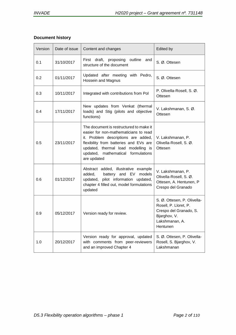
Document history
Version Date of issue Content and changes Edited by
0.1 31/10/2017 First draft, proposing outline and
structure of the document S. Ø. Ottesen
0.2 01/11/2017 Updated after meeting with Pedro,
Hossein and Magnus S. Ø. Ottesen
0.3 10/11/2017 Integrated with contributions from Pol P. Olivella-Rosell, S. Ø.
Ottesen
0.4 17/11/2017
New updates from Venkat (thermal
loads) and Stig (pilots and objective
functions)
V. Lakshmanan, S. Ø.
Ottesen
0.5 23/11/2017
The document is restructured to make it
easier for non-mathematicians to read
it. Problem descriptions are added,
flexibility from batteries and EVs are
updated, thermal load modelling is
updated, mathematical formulations
are updated
V. Lakshmanan, P.
Olivella-Rosell, S. Ø.
Ottesen
0.6 01/12/2017
Abstract added, illustrative example
added, battery and EV models
updated, pilot information updated,
chapter 4 filled out, model formulations
updated
V. Lakshmanan, P.
Olivella-Rosell, S. Ø.
Ottesen, A. Hentunen, P
Crespo del Granado
0.9 05/12/2017 Version ready for review.
S. Ø. Ottesen, P. Olivella-
Rosell, P. Lloret, P.
Crespo del Granado, S.
Bjarghov, V.
Lakshmanan, A.
Hentunen
1.0 20/12/2017
Version ready for approval, updated
with comments from peer-reviewers
and an improved Chapter 4
S. Ø. Ottesen, P. Olivella-
Rosell, S. Bjarghov, V.
Lakshmanan

INVADE H2020 project – Grant agreement nº. 731148
D5.3 Flexibility operation algorithms – phase 1 Page 3 of 110
Peer reviewed by:
Partner Reviewer
SIN Jayaprakash Rajasekharan
GreenFlux Michel Bayings
Deliverable beneficiaries:
WP / Task
WP5 / Task 5.3 and 5.4
WP8 / Task T8.3
INVADE H2020 project – Grant agreement nº. 731148
D5.3 Flexibility operation algorithms – phase 1 Page 4 of 110
Table of contents
Executive summary .................................................................................................... 9
1 Introduction ........................................................................................................ 10
2 Problem description and modelling concepts ................................................. 11
2.1 An illustrative example 11 2.2 Flexibility services for the DSO 15 2.3 Flexibility services for Prosumers 16 2.4 Prosumer and site 17 2.5 Flexibility 18
2.5.1 Flexibility from batteries 19
2.5.2 Flexibility from loads 24
2.5.3 Flexibility from EVs 30
2.5.4 Flexibility from generation units 33
2.5.5 Flexibility from aggregated resources 34
2.6 EV flexibility models 37
2.6.1 EV flexibility in households 39
2.6.2 EV flexibility in multiple charging points 39
2.6.3 EV flexibility in public charging sites 40
2.6.4 EV flexibility in V2X charging stations 40
3 Pilot sites ............................................................................................................ 41
3.1 Norway 41
3.1.1 Introduction 41
3.1.2 Roles and their interrelations 41
3.1.3 Resources and their interrelations and constraints 42
3.1.4 Contracts and prices 44
3.2 The Netherlands 47
3.2.1 Introduction 47
3.2.2 Roles and their interrelations 48
3.2.3 Resources and their interrelations and constraints 52
3.2.4 Contracts and prices 59
3.2.5 Objectives 61
3.3 Spain 62
3.3.5 Objective 65
INVADE H2020 project – Grant agreement nº. 731148
D5.3 Flexibility operation algorithms – phase 1 Page 5 of 110
3.4 Germany 65
4 Uncertainty, information structure and the planning process ........................ 66
4.1 Problem description 66 4.2 Uncertainty and information revelation 67
4.2.1 Solar PV production 67
4.2.2 Consumption at load limits 69
4.2.3 Aggregated consumption of load units 70
4.2.4 Consumption at a site 70
4.2.5 Consumption at a charging point 71
4.2.6 Prices 73
4.2.7 Flexibility request from a DSO 74
4.3 Possible planning approaches 74
4.3.1 Robust optimization technique 75
4.3.2 Stochastic programming 76
4.3.3 Rolling horizon deterministic planning 76
4.3.4 Rule-based method 78
4.4 The information structure 78 4.5 Length of the planning horizon 80 4.6 Time resolution 82
4.6.1 Prosumer 83
4.6.2 DSO 83
4.6.3 BRP 84
4.7 Overall operational scheduling optimization process 84
5 Mathematical formulations ................................................................................ 85
5.1 Overview of sets, parameters and variables 85
5.1.1 Sets 85
5.1.2 Parameters 86
5.1.3 Variables 89
5.2 Common/general constraints 90
5.2.1 Battery models 90
5.2.2 Load models 92
5.2.3 EV models 96
5.2.4 Generator models 102
5.2.5 Aggregated flexibility models 102

INVADE H2020 project – Grant agreement nº. 731148
D5.3 Flexibility operation algorithms – phase 1 Page 6 of 110
5.3 Specific models for DSO services 103
5.3.1 Objective function 103
5.3.2 DSO services specific constraints 103
5.4 Specific models for Prosumer services 105
5.4.1 Objective function(s) and pilot specific constraints for
prosumer services 105
5.4.2 Prosumer services specific constraints 107
References .............................................................................................................. 109

INVADE H2020 project – Grant agreement nº. 731148
D5.3 Flexibility operation algorithms – phase 1 Page 7 of 110
Abbreviations and Acronyms
Acronym Description
AHES AMI Head End system
API Application programming interface
BMS Battery Management System
BRP Balance Responsible Party
BS Balance Scheduling
CEM Customer energy management system
CPO Charge point operator
DER Distributed Energy Resources
DMS Distribution management system
DSO Distribution System Operator
EMG Energy Management Gateway
EV Electric Vehicle
EVSE Electric Vehicle Supply Equipment
FEP Front End Processor
FO Flexibility Operator
IEC International Electrotechnical Commission
IED Intelligent Electronic Device
IIP Integrated INVADE Platform
LV Low Voltage
MDC Meter Data Concentrator
MDM Meter data management
MR Meter Reader
MV Medium Voltage
NA Not Applicable
OCHP Open Clearing House Protocol
OCPI Open Charge Point Interface
OCPP Open Charge Point Protocol
OM Operation meter
OSCP Open Smart Charging Protocol
PRIME PoweRline Intelligent Metering Evolution
PV Photovoltaic
INVADE H2020 project – Grant agreement nº. 731148
D5.3 Flexibility operation algorithms – phase 1 Page 8 of 110
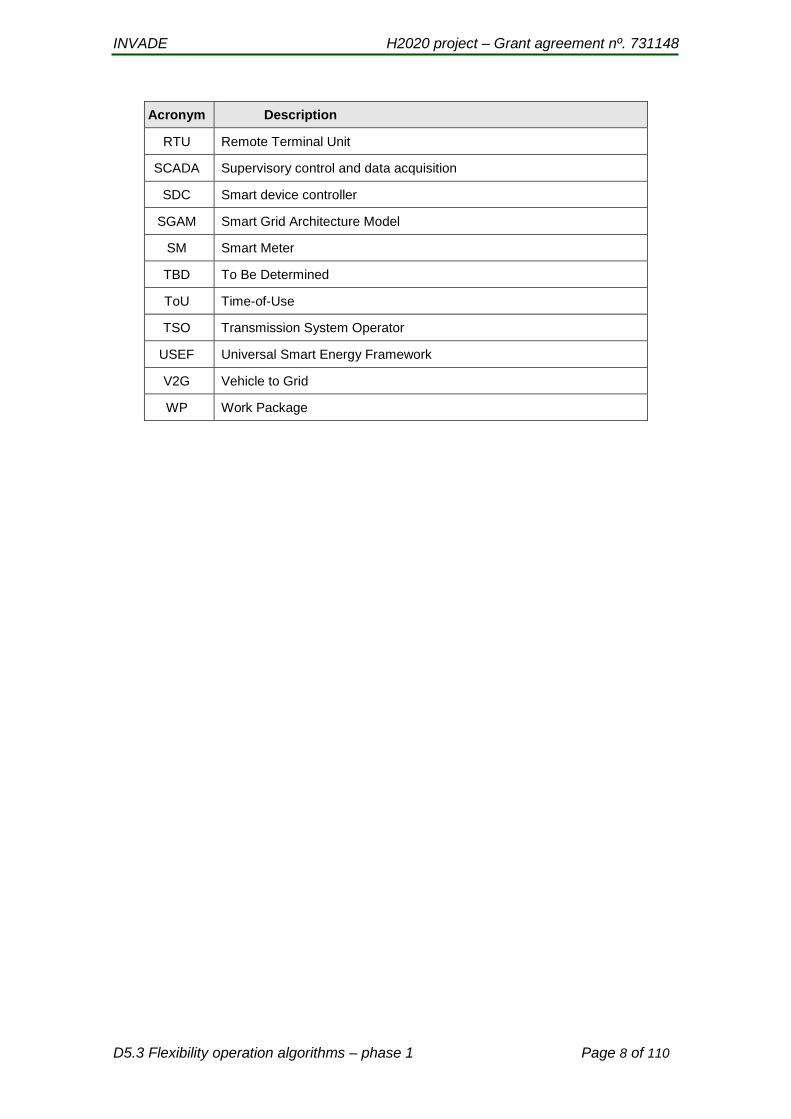
Acronym Description
RTU Remote Terminal Unit
SCADA Supervisory control and data acquisition
SDC Smart device controller
SGAM Smart Grid Architecture Model
SM Smart Meter
TBD To Be Determined
ToU Time-of-Use
TSO Transmission System Operator
USEF Universal Smart Energy Framework
V2G Vehicle to Grid
WP Work Package

INVADE H2020 project – Grant agreement nº. 731148
D5.3 Flexibility operation algorithms – phase 1 Page 9 of 110
Executive summary
A central deliverable in the INVADE project is the Integrated INVADE platform, which will
be developed in WP8. The platform will support many different functional areas, but the
main development in the INVADE project is the cloud based flexibility management
system, which will be used in the daily operations of the different flexibility services. A
first, simplified version of this system will be delivered to the pilots in June 2018.
This document contains a description of the algorithms that will be used in the daily
operations. First, the problem is described, and basic modelling concepts are proposed
and discussed with regards to flexibility from stationary batteries, loads, EVs and
generation. Then the pilots are described with the target to analyse of how their technical
and commercial setup will influence the design of the flexibility algorithms. This is
followed by a discussion of possible approaches for handling uncertainty, including the
length of the planning horizon and how detailed the time resolution should be. Finally,
the first version of the mathematical formulations is given.
A key finding in the document is that the way to model flexibility and how much value
that can be extracted from the flexible sources, are tightly connected to the amount of
information that is available. This challenge must be addressed in other WPs and tasks.
INVADE H2020 project – Grant agreement nº. 731148
D5.3 Flexibility operation algorithms – phase 1 Page 10 of 110
1 Introduction
According to the DoA the deliverable D5.3 Simplified Battery operation and control
algorithm contains the first version of flexibility management allocation and operation
algorithms worked out in two tasks: T5.3 Energy storage units allocation/positioning and
sizing algorithm and T5.4 Design and program the flexibility management operation
algorithm. The current document covers the part connected to T5.4, whereas D5.3
Optimal Placement and Sizing of Batteries in Low Voltage Grids covers the part
connected to T5.3.
The work in this document is built upon the content in several other deliverables in
different work packages: D4.1, D4.2, D5.1, D5.2 and D10.1.
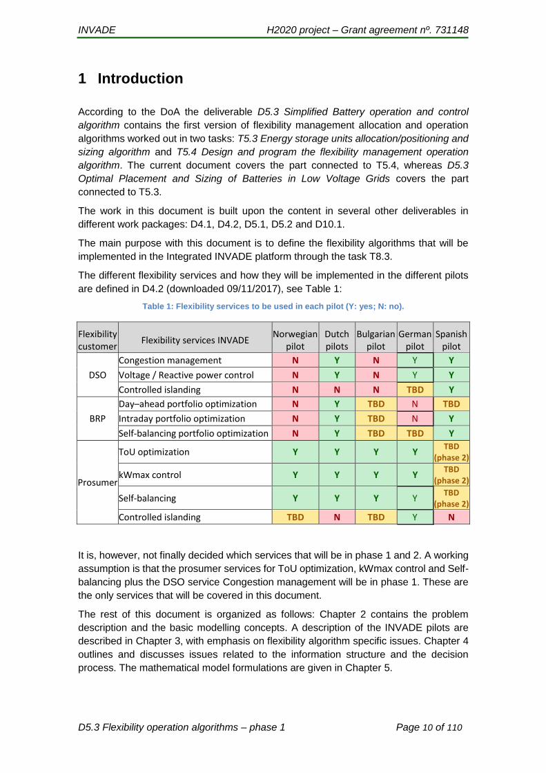
The main purpose with this document is to define the flexibility algorithms that will be
implemented in the Integrated INVADE platform through the task T8.3.
The different flexibility services and how they will be implemented in the different pilots
are defined in D4.2 (downloaded 09/11/2017), see Table 1:
Table 1: Flexibility services to be used in each pilot (Y: yes; N: no).
Flexibility customer
Flexibility services INVADE Norwegian
pilot Dutch pilots
Bulgarian pilot
German pilot
Spanish pilot
DSO
Congestion management N Y N Y Y
Voltage / Reactive power control N Y N Y Y
Controlled islanding N N N TBD Y
BRP
Day–ahead portfolio optimization N Y TBD N TBD
Intraday portfolio optimization N Y TBD N Y
Self-balancing portfolio optimization N Y TBD TBD Y
Prosumer
ToU optimization Y Y Y Y TBD
(phase 2)
kWmax control Y Y Y Y TBD
(phase 2)
Self-balancing Y Y Y Y TBD
(phase 2)
Controlled islanding TBD N TBD Y N
It is, however, not finally decided which services that will be in phase 1 and 2. A working
assumption is that the prosumer services for ToU optimization, kWmax control and Self-
balancing plus the DSO service Congestion management will be in phase 1. These are
the only services that will be covered in this document.
The rest of this document is organized as follows: Chapter 2 contains the problem
description and the basic modelling concepts. A description of the INVADE pilots are
described in Chapter 3, with emphasis on flexibility algorithm specific issues. Chapter 4
outlines and discusses issues related to the information structure and the decision
process. The mathematical model formulations are given in Chapter 5.

INVADE H2020 project – Grant agreement nº. 731148
D5.3 Flexibility operation algorithms – phase 1 Page 11 of 110
2 Problem description and modelling concepts
2.1 An illustrative example
This section contains a specific and simplified example aiming at giving the reader an
overall idea about the problems that this document address.
Consider a household with the following resources:
A PV panel
A set of inflexible loads
Two EV charging points
A stationary battery
A main meter that meters the net exchange with the grid, i.e. the purchase and the
sales
Separate meters for the PV panel, for each of the charging points and for the
battery
Since the household both produces and consumes electricity, it is a prosumer.
Figure 1. The prosumer with resources (circles) and meters (squares)
The prosumer has three flexible resources:
The EV charging points, where the power levels can be controlled continuously
between 0 and 4 kW
The battery, which can be charged and discharged with power levels between 0
and 4 kW. The energy levels can be between 0 and 10 kWh
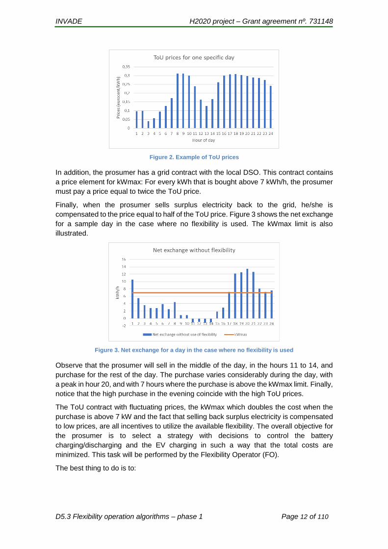
Further, assume that the prosumer has a contract with an electricity supplier, also
denoted a retailer, with prices that vary hour by hour (ToU) according to prices at the
Day-ahead market. We consider one given day, where the prices fluctuate according to
Figure 2.
INVADE H2020 project – Grant agreement nº. 731148
D5.3 Flexibility operation algorithms – phase 1 Page 12 of 110
Figure 2. Example of ToU prices
In addition, the prosumer has a grid contract with the local DSO. This contract contains
a price element for kWmax: For every kWh that is bought above 7 kWh/h, the prosumer
must pay a price equal to twice the ToU price.
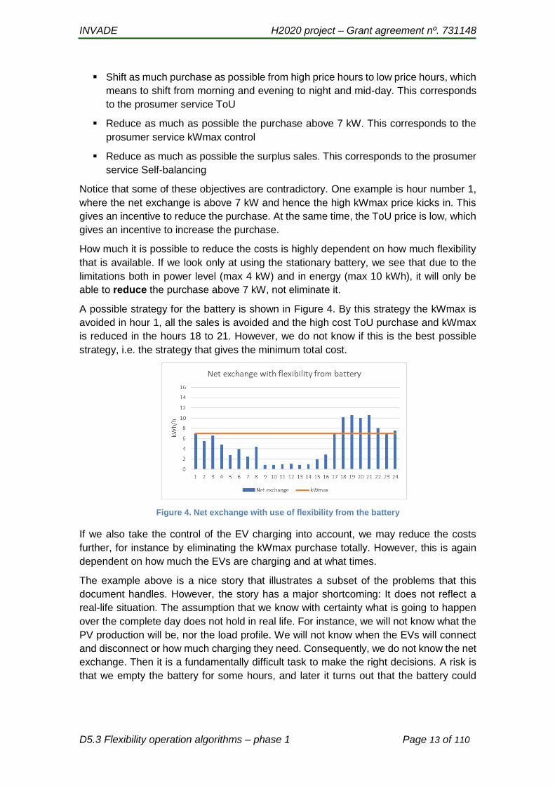
Finally, when the prosumer sells surplus electricity back to the grid, he/she is
compensated to the price equal to half of the ToU price. Figure 3 shows the net exchange
for a sample day in the case where no flexibility is used. The kWmax limit is also
illustrated.
Figure 3. Net exchange for a day in the case where no flexibility is used
Observe that the prosumer will sell in the middle of the day, in the hours 11 to 14, and
purchase for the rest of the day. The purchase varies considerably during the day, with
a peak in hour 20, and with 7 hours where the purchase is above the kWmax limit. Finally,
notice that the high purchase in the evening coincide with the high ToU prices.
The ToU contract with fluctuating prices, the kWmax which doubles the cost when the
purchase is above 7 kW and the fact that selling back surplus electricity is compensated
to low prices, are all incentives to utilize the available flexibility. The overall objective for
the prosumer is to select a strategy with decisions to control the battery
charging/discharging and the EV charging in such a way that the total costs are
minimized. This task will be performed by the Flexibility Operator (FO).
The best thing to do is to:
INVADE H2020 project – Grant agreement nº. 731148
D5.3 Flexibility operation algorithms – phase 1 Page 13 of 110
Shift as much purchase as possible from high price hours to low price hours, which
means to shift from morning and evening to night and mid-day. This corresponds
to the prosumer service ToU
Reduce as much as possible the purchase above 7 kW. This corresponds to the
prosumer service kWmax control
Reduce as much as possible the surplus sales. This corresponds to the prosumer
service Self-balancing
Notice that some of these objectives are contradictory. One example is hour number 1,
where the net exchange is above 7 kW and hence the high kWmax price kicks in. This
gives an incentive to reduce the purchase. At the same time, the ToU price is low, which
gives an incentive to increase the purchase.
How much it is possible to reduce the costs is highly dependent on how much flexibility
that is available. If we look only at using the stationary battery, we see that due to the
limitations both in power level (max 4 kW) and in energy (max 10 kWh), it will only be
able to reduce the purchase above 7 kW, not eliminate it.
A possible strategy for the battery is shown in Figure 4. By this strategy the kWmax is
avoided in hour 1, all the sales is avoided and the high cost ToU purchase and kWmax
is reduced in the hours 18 to 21. However, we do not know if this is the best possible
strategy, i.e. the strategy that gives the minimum total cost.
Figure 4. Net exchange with use of flexibility from the battery
If we also take the control of the EV charging into account, we may reduce the costs
further, for instance by eliminating the kWmax purchase totally. However, this is again
dependent on how much the EVs are charging and at what times.
The example above is a nice story that illustrates a subset of the problems that this
document handles. However, the story has a major shortcoming: It does not reflect a
real-life situation. The assumption that we know with certainty what is going to happen
over the complete day does not hold in real life. For instance, we will not know what the
PV production will be, nor the load profile. We will not know when the EVs will connect
and disconnect or how much charging they need. Consequently, we do not know the net
exchange. Then it is a fundamentally difficult task to make the right decisions. A risk is
that we empty the battery for some hours, and later it turns out that the battery could
INVADE H2020 project – Grant agreement nº. 731148
D5.3 Flexibility operation algorithms – phase 1 Page 14 of 110
have provided higher value if it was fully charged. So, the best strategy would have been
to wait with the discharging.
One way of dealing with information we do not have, is to make predictions and to make
decision based on these. For production and consumption, the nature of the predictions
will be so that they may be quite good for the coming minutes or hours, but the further
out into the future we get, the larger the prediction errors will be. This might be handled
by repeatedly updating the predictions and rerunning the decision model. For instance,
we could update the predictions each hour, we could make new decisions each hour,
and each time we only implement the decisions for the nearest hour. However, when
making the decisions, we look at the whole day, to reduce the risk of making “wrong”
decisions.
To be able to do this, we need a suitable decision support model. In this document we
use mathematical programming, also called optimization, which deals with problems
where one seeks to maximize or minimize a real function by choosing the values of
variables from an allowed set. In our small example, we seek to minimize the total cost.
This is the objective, formulated in the objective function. An applicable model must also
reflect all the technical constraints, for example the battery’s limitation in maximum
charging and discharging power of 4 kW, and the maximum capacity of 10 kWh.
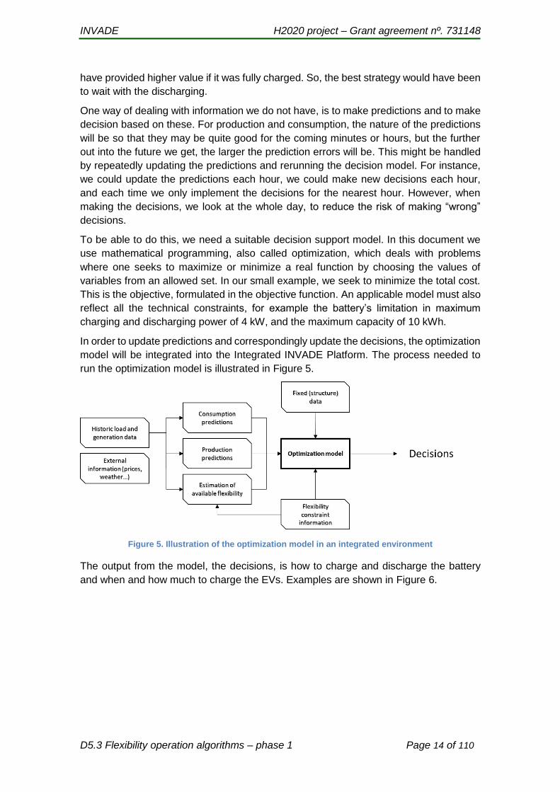
In order to update predictions and correspondingly update the decisions, the optimization
model will be integrated into the Integrated INVADE Platform. The process needed to
run the optimization model is illustrated in Figure 5.
Figure 5. Illustration of the optimization model in an integrated environment
The output from the model, the decisions, is how to charge and discharge the battery
and when and how much to charge the EVs. Examples are shown in Figure 6.

INVADE H2020 project – Grant agreement nº. 731148
D5.3 Flexibility operation algorithms – phase 1 Page 15 of 110
Figure 6. Examples of decisions for battery and EV1 for one day
As we saw in the example, one issue is how to detect the need for flexibility usage, since
the net exchange is the basis for the decisions. Another issue is how to know how much
flexibility that is available. For the battery it is quite easy, since we have full control of
charging and probably have access to meter values for the energy level. For the EVs it
is a bit more complicated. First of all, we most likely do not know in advance when they
will connect and disconnect, or how much charging they need. However, apps might be
used to increase the level of information. Perhaps other information channels can be
used in addition to predictions. Anyway, it is clear that the more information we have
available, the smarter decisions we can make.
2.2 Flexibility services for the DSO
In this document, the flexibility service congestion management is included as the only
service for the DSO. According to D4.1 Overall INVADE architecture, congestion
management is defined as follows:
Congestion management refers to avoiding the thermal overload of system components
by reducing peak loads where failure due to overloading may occur. The conventional
solution is grid reinforcement (e.g., cables, transformers). The alternative (load flexibility)
may defer or even avoid the necessity of grid investments.
The congestion management service in the INVADE project is based on the EMPOWER-
concept as described in [1]. The DSO requests activation of flexibility when needed, for
instance in cases where a substation is overloaded. The Flexibility Operator (FO)
delivers the requested flexibility provided by a portfolio of prosumers with flexible
resources, see Figure 7.

INVADE H2020 project – Grant agreement nº. 731148
D5.3 Flexibility operation algorithms – phase 1 Page 16 of 110
Figure 7. Congestion management services delivered to the DSO
The FO’s problem is to generate a plan for when and how much to activate the different
flexibility resources in such a way that:
The request from the DSO is met
No constraint is violated
The activation is done to the minimum cost
2.3 Flexibility services for Prosumers
According to D4.1 Overall INVADE architecture, the prosumer services covered in this
document are defined as:
ToU optimization is based on load shifting from high-price intervals to low-price intervals
or even complete load shedding during periods with high prices. This optimization
requires that tariff schedules are known in advance (e.g., day-ahead) and will lower the
Prosumer’s energy bill.
kWmax control is based on reducing the maximum load (peak shaving) that the
Prosumer consumes within a predefined duration (e.g., month, year), either through load
shifting or shedding. Current tariff schemes, especially for C&I customers, often include
a tariff component that is based on the Prosumer’s maximum load (kWmax). By reducing
this maximum load, the Prosumer can save on tariff costs. For the DSO, this kWmax
component is a rudimentary form of demand-side management.
Self-balancing is typical for Prosumers who also generate electricity (for example,
through solar PV or CHP systems). Value is created through the difference in the prices
of buying, generating, and selling electricity (including taxation if applicable). Note that
solar PV self-balancing is not meaningful where national regulations allow for
administrative balancing of net load and net generation.
Which roles that are involved in the prosumer services, will vary from case to case. The
incentives for ToU, kWmax and self-balancing can come from a combination of terms in
INVADE H2020 project – Grant agreement nº. 731148
D5.3 Flexibility operation algorithms – phase 1 Page 17 of 110
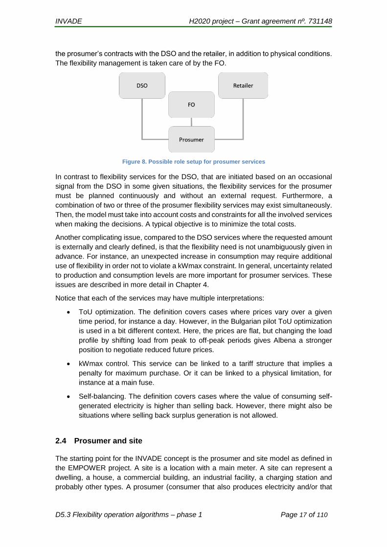
the prosumer’s contracts with the DSO and the retailer, in addition to physical conditions.
The flexibility management is taken care of by the FO.
Figure 8. Possible role setup for prosumer services
In contrast to flexibility services for the DSO, that are initiated based on an occasional
signal from the DSO in some given situations, the flexibility services for the prosumer
must be planned continuously and without an external request. Furthermore, a
combination of two or three of the prosumer flexibility services may exist simultaneously.
Then, the model must take into account costs and constraints for all the involved services
when making the decisions. A typical objective is to minimize the total costs.
Another complicating issue, compared to the DSO services where the requested amount
is externally and clearly defined, is that the flexibility need is not unambiguously given in
advance. For instance, an unexpected increase in consumption may require additional
use of flexibility in order not to violate a kWmax constraint. In general, uncertainty related
to production and consumption levels are more important for prosumer services. These
issues are described in more detail in Chapter 4.
Notice that each of the services may have multiple interpretations:
ToU optimization. The definition covers cases where prices vary over a given
time period, for instance a day. However, in the Bulgarian pilot ToU optimization
is used in a bit different context. Here, the prices are flat, but changing the load
profile by shifting load from peak to off-peak periods gives Albena a stronger
position to negotiate reduced future prices.
kWmax control. This service can be linked to a tariff structure that implies a
penalty for maximum purchase. Or it can be linked to a physical limitation, for
instance at a main fuse.
Self-balancing. The definition covers cases where the value of consuming self-
generated electricity is higher than selling back. However, there might also be
situations where selling back surplus generation is not allowed.
2.4 Prosumer and site
The starting point for the INVADE concept is the prosumer and site model as defined in
the EMPOWER project. A site is a location with a main meter. A site can represent a
dwelling, a house, a commercial building, an industrial facility, a charging station and
probably other types. A prosumer (consumer that also produces electricity and/or that
INVADE H2020 project – Grant agreement nº. 731148
D5.3 Flexibility operation algorithms – phase 1 Page 18 of 110
provides flexibility) is a legal entity (person or business), and a site must have one
prosumer connected to it. Prosumers can move in and out from a site, but at a specific
time only one prosumer can be active.
As stated above, each site will have a main meter, which is the basis for the grid contract
with the DSO and the retail contract with the chosen retailer. In addition, a site can have
one or several resources, where each resource is categorized in one and only one out
of four types:
Generator resources
Load resources
Electric vehicles (EVs)
Storages
Each resource can be a single appliance or a virtual collection of several appliances or
circuits. Furthermore, each resource can be metered or not and controllable or not. Meter
values from the main meter (net energy in and out) and from the sub meters (at the
resource level) will be collected in real time with fine time granulation (currently each 10
seconds in the EMPOWER project). Which control options that exist will depend both on
the technical characteristics of each resource/control equipment and on the agreement
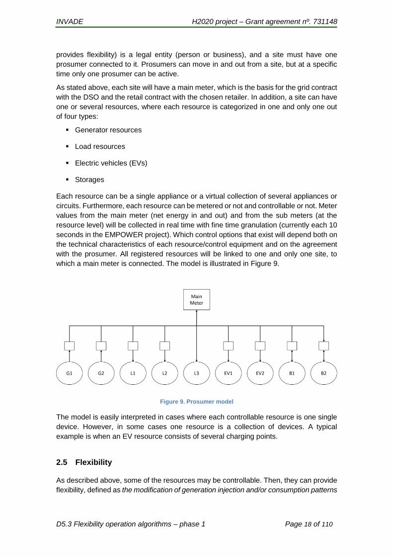
with the prosumer. All registered resources will be linked to one and only one site, to
which a main meter is connected. The model is illustrated in Figure 9.
Figure 9. Prosumer model
The model is easily interpreted in cases where each controllable resource is one single
device. However, in some cases one resource is a collection of devices. A typical
example is when an EV resource consists of several charging points.
2.5 Flexibility
As described above, some of the resources may be controllable. Then, they can provide
flexibility, defined as the modification of generation injection and/or consumption patterns

INVADE H2020 project – Grant agreement nº. 731148
D5.3 Flexibility operation algorithms – phase 1 Page 19 of 110
in reaction to an external price or activation signal in order to provide a service within the
electrical system [2].
Our objective is to utilize the flexibility to meet different objectives without violating
constraints. Below, a description of possible flexibility characteristics is described for
each resource type. Later, in Chapter 4.1, the different characteristics are formulated
mathematically.
The starting point for the flexibility descriptions are from [3], which are further developed
in the EMPOWER project [1]. However, it is expected that the descriptions will be refined
and adapted through the work in INVADE.
Since flexibility is defined as “a modification”, it must be compared to some baseline,
which for instance can be an original schedule or a prediction. The flexibility is then the
difference between the baseline and the revised plan, see Figure 10.
Assume the blue bars represent a baseline consumption and that the orange line
represents the revised plan. Then, we have flexibility provision in period 4 and 8, equal
to 5 kW.
The provision of flexibility is called regulation, which can come in two directions: Up and
down. Up-regulation means increased production or decreased consumption, while
down-regulation means decreased production or increased consumption.
Figure 10. Original and revised schedule and the provision of flexibility
Focus on flexibility provision directly is important in cases where flexibility is sold and
bought as a service, for instance to the DSO.
2.5.1 Flexibility from batteries
Batteries provide high flexibility as they are fully dedicated to this task. An example is
shown in Figure 11, where a battery provides energy and stores energy in different time
periods to offer some requested service by a prosumer or a FO. The battery has a certain
energy capacity storage limit and a charge and discharge power limit.

INVADE H2020 project – Grant agreement nº. 731148
D5.3 Flexibility operation algorithms – phase 1 Page 20 of 110
Figure 11. Battery flexibility example
Batteries are electrochemical energy storages with complex nonlinear characteristics
and interdependencies. The most important characteristics are the capacity, open-circuit
voltage (OCV), and internal impedance, which also dictate the energy capacity, efficiency
and power capability. Moreover, batteries are very sensitive to temperature. Too low
temperature results in poor performance and low efficiency, while too high temperature
results in increased rate of degradation and even decomposition and safety risks. All
these characteristics cause constraints and limitations for the usage in order to achieve
safe operation and long lifetime. The battery characteristics are explained in more detail
in D6.1 Storage system dimensioning and design tool.
Each battery chemistry has a unique OCV curve and a voltage window. The specified
maximum and minimum voltages should not be exceeded in any case as it may cause
increased rate of degradation and even cell decomposition and permanent damage.
Therefore, high and low cutoff voltage are specified for each cell to ensure safe operation
and long lifetime. The controller algorithm must be capable to prevent the voltage to
reach these cutoff voltages during use. This can be implemented by setting limitations
for the usable SOC (state-of-charge) window as well as discharge power when
approaching fully discharged state and charge power when approaching fully charged
state.
During loading, polarization losses occur when a load current passes through the
electrodes. These polarization losses consist of ohmic polarization, activation
polarization and concentration polarization. The presence of these losses can be seen
as a difference between the OCV and the terminal voltage during loading. As the
polarization effects increase with increasing current, the low cutoff voltage is reached
earlier when discharging with higher rates. This is known as the rate effect. However, the
capacity is not lost, but is usable once the voltage has recovered. Full relaxation takes
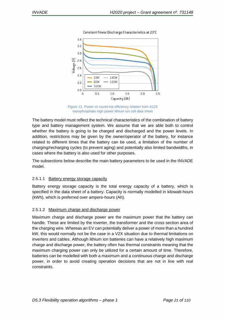
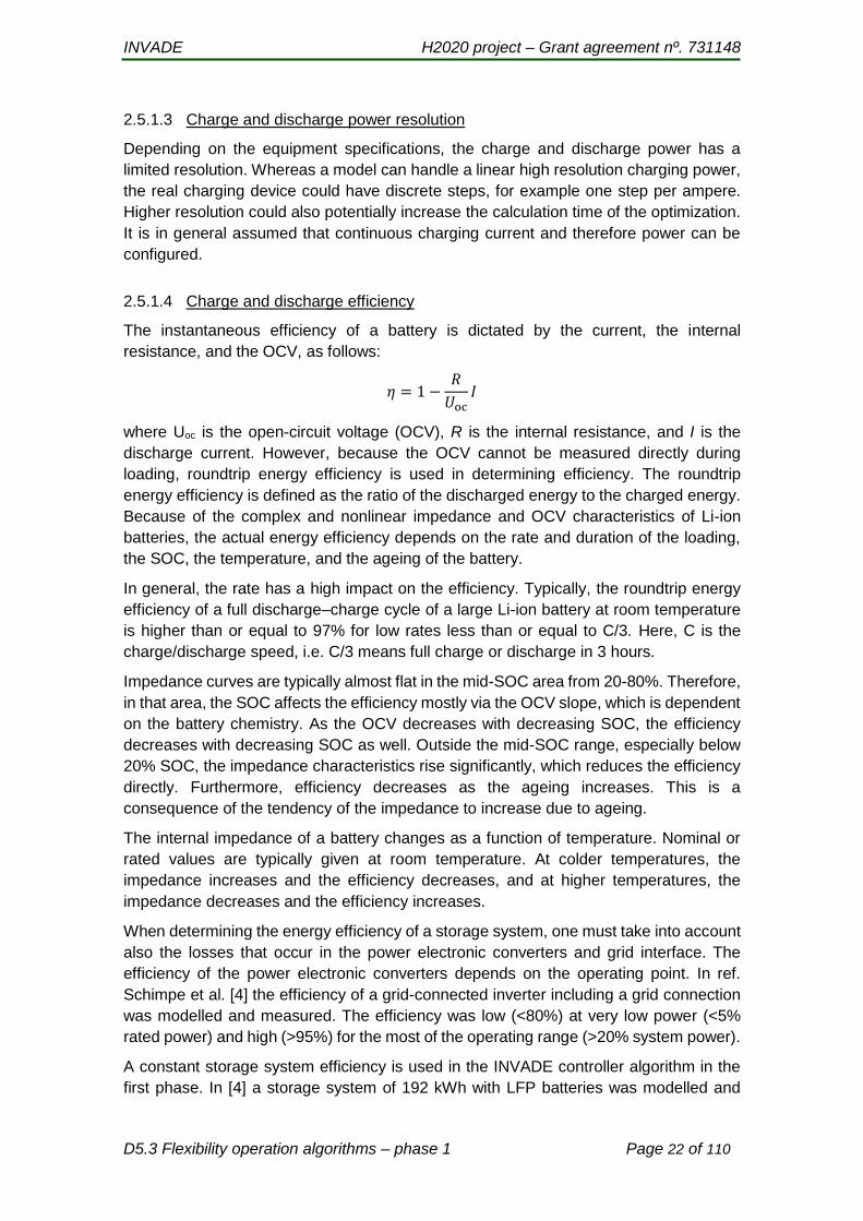
hours to complete. Rate effect is illustrated in Figure 12 , which shows an A123 lithium-
ion cell performance under different power extractions. The area below the curve is the
total energy extracted, and it is smaller as the power extracted increases.
INVADE H2020 project – Grant agreement nº. 731148
D5.3 Flexibility operation algorithms – phase 1 Page 21 of 110
Figure 12. Power vs round-trip efficiency relation from A123
nanophosphate high power lithium ion cell data sheet
The battery model must reflect the technical characteristics of the combination of battery
type and battery management system. We assume that we are able both to control
whether the battery is going to be charged and discharged and the power levels. In
addition, restrictions may be given by the owner/operator of the battery, for instance
related to different times that the battery can be used, a limitation of the number of
charging/recharging cycles (to prevent aging) and potentially also limited bandwidths, in
cases where the battery is also used for other purposes.
The subsections below describe the main battery parameters to be used in the INVADE
model.
2.5.1.1 Battery energy storage capacity
Battery energy storage capacity is the total energy capacity of a battery, which is
specified in the data sheet of a battery. Capacity is normally modelled in kilowatt-hours
(kWh), which is preferred over ampere-hours (Ah).
2.5.1.2 Maximum charge and discharge power
Maximum charge and discharge power are the maximum power that the battery can
handle. These are limited by the inverter, the transformer and the cross section area of
the charging wire. Whereas an EV can potentially deliver a power of more than a hundred
kW, this would normally not be the case in a V2X situation due to thermal limitations on
inverters and cables. Although lithium ion batteries can have a relatively high maximum
charge and discharge power, the battery often has thermal constraints meaning that the
maximum charging power can only be utilized for a certain amount of time. Therefore,
batteries can be modelled with both a maximum and a continuous charge and discharge
power, in order to avoid creating operation decisions that are not in line with real
constraints.
INVADE H2020 project – Grant agreement nº. 731148
D5.3 Flexibility operation algorithms – phase 1 Page 22 of 110
2.5.1.3 Charge and discharge power resolution
Depending on the equipment specifications, the charge and discharge power has a
limited resolution. Whereas a model can handle a linear high resolution charging power,
the real charging device could have discrete steps, for example one step per ampere.
Higher resolution could also potentially increase the calculation time of the optimization.
It is in general assumed that continuous charging current and therefore power can be
configured.
2.5.1.4 Charge and discharge efficiency
The instantaneous efficiency of a battery is dictated by the current, the internal
resistance, and the OCV, as follows:
𝜂 = 1 −𝑅
𝑈oc𝐼
where Uoc is the open-circuit voltage (OCV), R is the internal resistance, and I is the
discharge current. However, because the OCV cannot be measured directly during
loading, roundtrip energy efficiency is used in determining efficiency. The roundtrip
energy efficiency is defined as the ratio of the discharged energy to the charged energy.
Because of the complex and nonlinear impedance and OCV characteristics of Li-ion
batteries, the actual energy efficiency depends on the rate and duration of the loading,
the SOC, the temperature, and the ageing of the battery.
In general, the rate has a high impact on the efficiency. Typically, the roundtrip energy
efficiency of a full discharge–charge cycle of a large Li-ion battery at room temperature
is higher than or equal to 97% for low rates less than or equal to C/3. Here, C is the
charge/discharge speed, i.e. C/3 means full charge or discharge in 3 hours.
Impedance curves are typically almost flat in the mid-SOC area from 20-80%. Therefore,
in that area, the SOC affects the efficiency mostly via the OCV slope, which is dependent
on the battery chemistry. As the OCV decreases with decreasing SOC, the efficiency
decreases with decreasing SOC as well. Outside the mid-SOC range, especially below
20% SOC, the impedance characteristics rise significantly, which reduces the efficiency
directly. Furthermore, efficiency decreases as the ageing increases. This is a
consequence of the tendency of the impedance to increase due to ageing.
The internal impedance of a battery changes as a function of temperature. Nominal or
rated values are typically given at room temperature. At colder temperatures, the
impedance increases and the efficiency decreases, and at higher temperatures, the
impedance decreases and the efficiency increases.
When determining the energy efficiency of a storage system, one must take into account
also the losses that occur in the power electronic converters and grid interface. The
efficiency of the power electronic converters depends on the operating point. In ref.
Schimpe et al. [4] the efficiency of a grid-connected inverter including a grid connection
was modelled and measured. The efficiency was low (<80%) at very low power (<5%
rated power) and high (>95%) for the most of the operating range (>20% system power).
A constant storage system efficiency is used in the INVADE controller algorithm in the
first phase. In [4] a storage system of 192 kWh with LFP batteries was modelled and
INVADE H2020 project – Grant agreement nº. 731148
D5.3 Flexibility operation algorithms – phase 1 Page 23 of 110
simulated for several different use strategies and scenarios. The optimum roundtrip
energy efficiency of 87% was obtained under constant cycling with partial load, while
most of the scenarios resulted in 70–80% roundtrip efficiencies. In INVADE pilots, the
base scenario is that a low rate is typically used, which results in high efficiency for the
battery and the inverter. Based on these findings, 85% will be used as the starting point
for the storage system roundtrip efficiency. This equals to the discharge and charge
efficiency of 92%. However, the efficiency parameter can be adapted to each pilot. Low
power operation (less than 10% of system power) should be avoided due to relatively
low efficiency of the power electronics.
The pilot adaptations as well as more advanced methods to implement the efficiency
characteristics will be investigated in WP6, and the results will be adapted to the
controller algorithm in a later phase. One possibility is to set the efficiency parameters
outside the optimization algorithm before executing the algorithm.
2.5.1.5 Cost of degradation
Battery performance degrades as a result of ageing. The performance degradation can
be divided into capacity fading and power fading. Degradation happens to all batteries
regardless of whether they are used or not. Cycle ageing happens during discharging
and charging, while calendar ageing happens when the battery is not used. The rate of
degradation depends on the use profile, storage SOC and ambient conditions.
The models presented in this deliverable have no degradation cost taken into account.
However, this is implementable, and will be taken into account in a later phase. The
degradation mechanisms are very complex and dependent on the use profile and
ambient conditions. These stress factors and their modelling methods are studied in
WP6, and the results will be included in the final controller algorithm.
2.5.1.6 Self-discharge coefficient
Self-discharge is not included in present models, but could easily be implemented. Self-
discharge is basically a battery losing state of charge slowly when not being used, where
all batteries have an own self-discharge coefficient depending on technology. Because
most batteries in the pilots are intended for daily or at least weekly use, self-discharge is
not the most important factor, but could in theory be included if considered to be relevant.
2.5.1.7 Capacity utilization factor
In power systems the control variable is typically power instead of current. At CV
(constant voltage) regions close to the cutoff voltages, maximum available power values
can be reduced to mimic CV operation.
During charging, the boundary between the normal operation and the voltage-limited
operation depends on the rate, the internal impedance, and the OCV characteristics.
Typical SOC values for the boundary at C/3, 1C, and 2C rates are 95%, 90%, 80%.
However, these numbers vary and depend especially on the cell chemistry.
During discharging, the actual boundary between the constant-current or constant-power
operation and the cutoff or CV operation is typically close to 0% SOC for discharging
INVADE H2020 project – Grant agreement nº. 731148
D5.3 Flexibility operation algorithms – phase 1 Page 24 of 110
with rates of less than 3C. Nevertheless, the power limiting region should start at around
10% SOC to prevent abrupt ending of the discharge due to accidentally reaching the
cutoff voltage. Also the efficiency starts to reduce significantly already before that, and
the heat generation rate increases rapidly as the SOC approaches 0%.
For full utilization of the battery performance without voltage-based limitations, a SOC
range that allows full-power operation can be defined. Moreover, this region can be
further reduced in order to take into account other aspects such as increased rate of
aging at high SOC and lower efficiency at low SOC.
2.5.2 Flexibility from loads
A load unit is an appliance or a virtual collection of appliances that consume electricity.
We split load units into three main classes: Inflexible, curtailable and shiftable. Inflexible
load units are devices that can not be controlled, for instance TVs or food cooking
appliances.
Curtailable load units can be disconnectable if the only options are to be on or completely
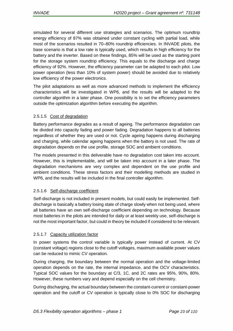
switched off. Or they can be reducible if the power levels can be controlled. Figure 13
shows a possible baseline consumption for load unit. If the load unit is inflexible, the
schedule will be equal to the baseline.
Figure 13. Baseline consumption for a load unit
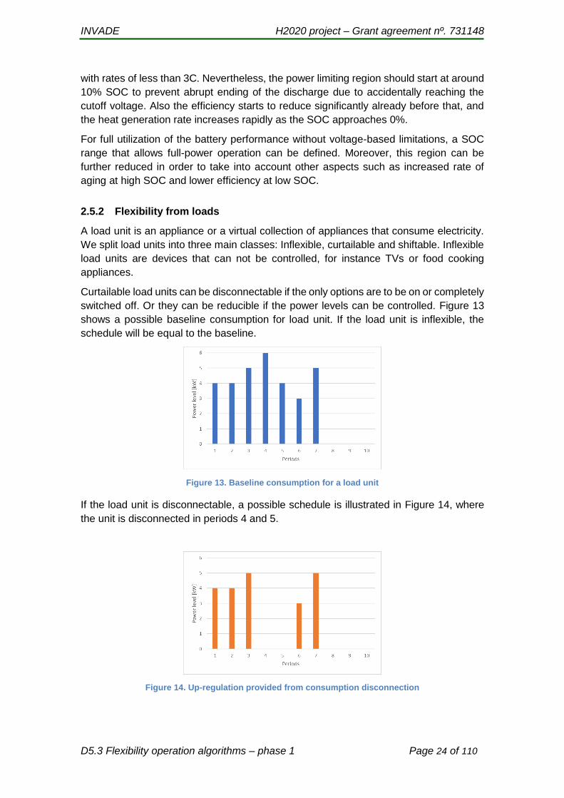
If the load unit is disconnectable, a possible schedule is illustrated in Figure 14, where
the unit is disconnected in periods 4 and 5.
Figure 14. Up-regulation provided from consumption disconnection
INVADE H2020 project – Grant agreement nº. 731148
D5.3 Flexibility operation algorithms – phase 1 Page 25 of 110
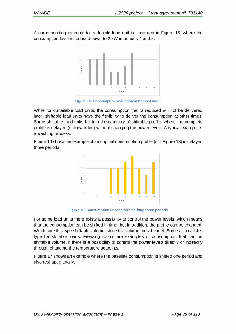
A corresponding example for reducible load unit is illustrated in Figure 15, where the
consumption level is reduced down to 2 kW in periods 4 and 5.
Figure 15. Consumption reduction in hours 4 and 5
While for curtailable load units, the consumption that is reduced will not be delivered
later, shiftable load units have the flexibility to deliver the consumption at other times.
Some shiftable load units fall into the category of shiftable profile, where the complete
profile is delayed (or forwarded) without changing the power levels. A typical example is
a washing process.
Figure 16 shows an example of an original consumption profile (still Figure 13) is delayed
three periods.
Figure 16. Consumption in case with shifting three periods
For some load units there exists a possibility to control the power levels, which means
that the consumption can be shifted in time, but in addition, the profile can be changed.
We denote this type shiftable volume, since the volume must be met. Some also call this
type for storable loads. Freezing rooms are examples of consumption that can be
shiftable volume, if there is a possibility to control the power levels directly or indirectly
through changing the temperature setpoints.
Figure 17 shows an example where the baseline consumption is shifted one period and
also reshaped totally.

INVADE H2020 project – Grant agreement nº. 731148
D5.3 Flexibility operation algorithms – phase 1 Page 26 of 110
Figure 17. Consumption in case with shifting and shaping
In order not to induce to large disadvantages for the prosumers and to keep inside
physical limits, it must be possible to limit the controllability of the different load units.
These constraints will be different between the different categories of flexibility:
Curtailable disconnectable: Curtailment is allowed only for certain periods. A curtailment
can have a maximum duration before it must be reconnected. After a reconnection, the
load unit must have a minimum rest time before the next disconnection.
Curtailable reducible: The limitations will be the same as for curtailable disconnectable.
In addition, the reduction must be within specified limits.
Shiftable profile: There must be limitations related to how much a consumption can be
shifted forward or backward, or in other words: earliest start and latest finish period.
Shiftable volume: Same limitations as shiftable profile. In addition, minimum and
maximum power levels must be defined.
Utilizing flexibility from load resources may induce added costs or discomfort for the
prosumers.
For curtailable load units, we have the foundational issue that we can not meter how
much we have curtailed. One approach is to estimate the volume curtailed and then
compensate according to prices per curtailed kWh. Another, more straightforward
approach, is to compensate based on the number of periods curtailed. In the EMPOWER
project the latter is chosen.
For shiftable load units, a natural approach is to compensate according to the length of
the delay, or in general: how long the consumption is moved away from the baseline. For
shiftable profile load units this is a straightforward strategy: You just count the number of
periods the start or the end is shifted and multiply with a price per period. For shiftable
volume load units, it is a bit more complicated. In the example in Figure 17 both the start
and the end is delayed with one period, so the delay is easy to handle here. However,
we also see that some of the consumption is shifted to earlier periods, so on average,
the volume is not delayed with one whole period. Other examples could be even more
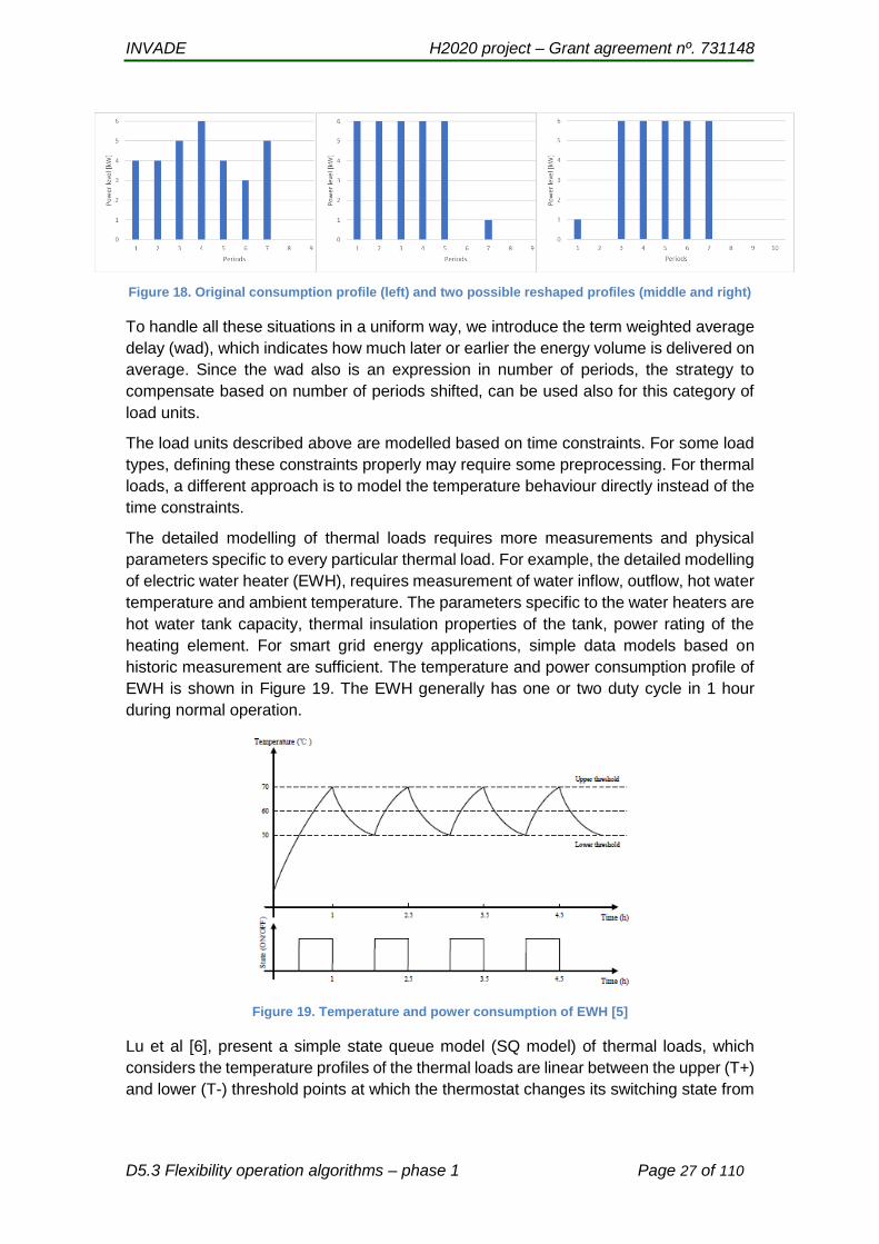
complicated, see Figure 18 that illustrates two possible new profiles where both the start
and end periods are the same (and hence, no delay), but where most of the consumption
is met earlier and later, respectively.
INVADE H2020 project – Grant agreement nº. 731148
D5.3 Flexibility operation algorithms – phase 1 Page 27 of 110
Figure 18. Original consumption profile (left) and two possible reshaped profiles (middle and right)
To handle all these situations in a uniform way, we introduce the term weighted average
delay (wad), which indicates how much later or earlier the energy volume is delivered on
average. Since the wad also is an expression in number of periods, the strategy to
compensate based on number of periods shifted, can be used also for this category of
load units.
The load units described above are modelled based on time constraints. For some load
types, defining these constraints properly may require some preprocessing. For thermal
loads, a different approach is to model the temperature behaviour directly instead of the
time constraints.
The detailed modelling of thermal loads requires more measurements and physical
parameters specific to every particular thermal load. For example, the detailed modelling
of electric water heater (EWH), requires measurement of water inflow, outflow, hot water
temperature and ambient temperature. The parameters specific to the water heaters are
hot water tank capacity, thermal insulation properties of the tank, power rating of the
heating element. For smart grid energy applications, simple data models based on
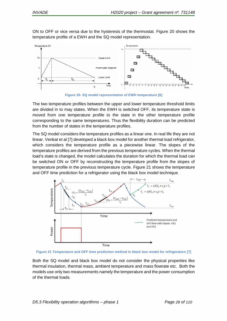
historic measurement are sufficient. The temperature and power consumption profile of
EWH is shown in Figure 19. The EWH generally has one or two duty cycle in 1 hour
during normal operation.
Figure 19. Temperature and power consumption of EWH [5]
Lu et al [6], present a simple state queue model (SQ model) of thermal loads, which
considers the temperature profiles of the thermal loads are linear between the upper (T+)
and lower (T-) threshold points at which the thermostat changes its switching state from
INVADE H2020 project – Grant agreement nº. 731148
D5.3 Flexibility operation algorithms – phase 1 Page 28 of 110
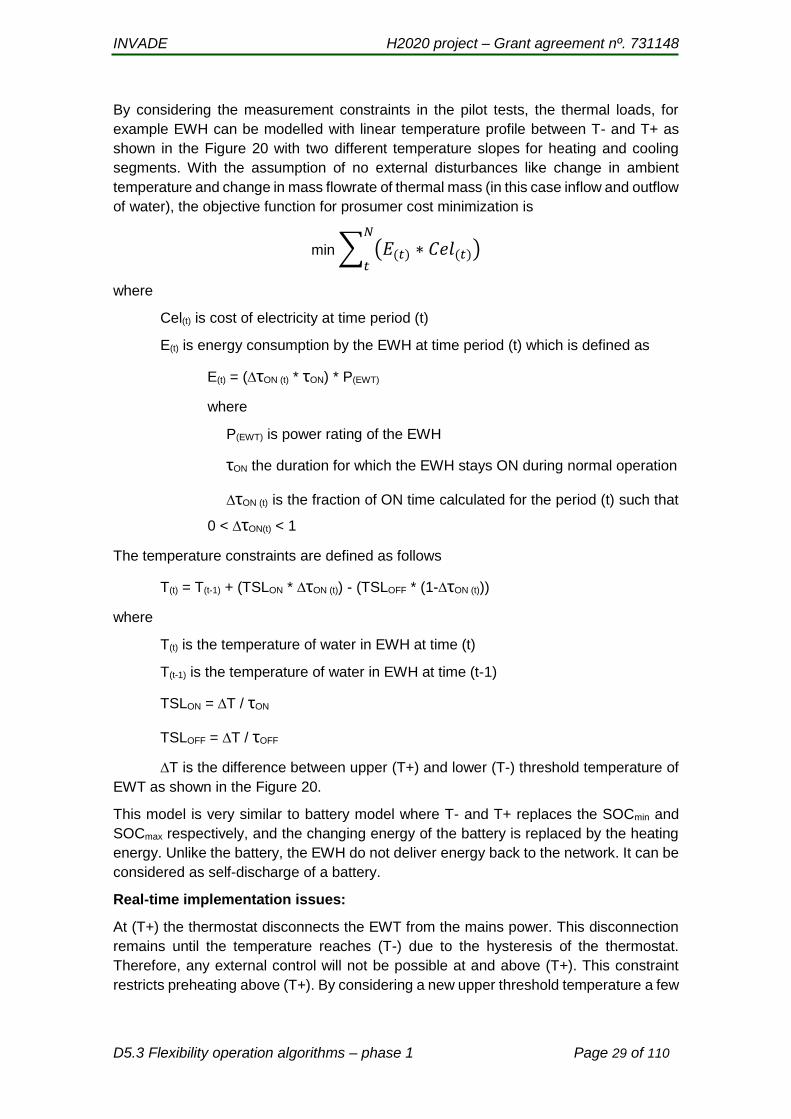
ON to OFF or vice versa due to the hysteresis of the thermostat. Figure 20 shows the
temperature profile of a EWH and the SQ model representation.
Figure 20. SQ model representation of EWH temperature [6]
The two temperature profiles between the upper and lower temperature threshold limits
are divided in to may states. When the EWH is switched OFF, its temperature state is
moved from one temperature profile to the state in the other temperature profile
corresponding to the same temperatures. Thus the flexibility duration can be predicted
from the number of states in the temperature profiles.
The SQ model considers the temperature profiles as a linear one. In real life they are not
linear. Venkat et al [7] developed a black box model for another thermal load refrigerator,
which considers the temperature profile as a piecewise linear. The slopes of the
temperature profiles are derived from the previous temperature cycles. When the thermal
load’s state is changed, the model calculates the duration for which the thermal load can
be switched ON or OFF by reconstructing the temperature profile from the slopes of
temperature profile in the previous temperature cycle. Figure 21 shows the temperature
and OFF time prediction for a refrigerator using the black box model technique.
Figure 21 Temperature and OFF time prediction method in black box model for refrigerators [7]
Both the SQ model and black box model do not consider the physical properties like
thermal insulation, thermal mass, ambient temperature and mass flowrate etc. Both the
models use only two measurements namely the temperature and the power consumption
of the thermal loads.
INVADE H2020 project – Grant agreement nº. 731148
D5.3 Flexibility operation algorithms – phase 1 Page 29 of 110
By considering the measurement constraints in the pilot tests, the thermal loads, for
example EWH can be modelled with linear temperature profile between T- and T+ as
shown in the Figure 20 with two different temperature slopes for heating and cooling
segments. With the assumption of no external disturbances like change in ambient
temperature and change in mass flowrate of thermal mass (in this case inflow and outflow
of water), the objective function for prosumer cost minimization is
min ∑ (𝐸(𝑡) ∗ 𝐶𝑒𝑙(𝑡))𝑁
𝑡
where
Cel(t) is cost of electricity at time period (t)
E(t) is energy consumption by the EWH at time period (t) which is defined as
E(t) = (∆τON (t) * τON) * P(EWT)
where
P(EWT) is power rating of the EWH
τON the duration for which the EWH stays ON during normal operation
∆τON (t) is the fraction of ON time calculated for the period (t) such that
0 < ∆τON(t) < 1
The temperature constraints are defined as follows
T(t) = T(t-1) + (TSLON * ∆τON (t)) - (TSLOFF * (1-∆τON (t)))
where
T(t) is the temperature of water in EWH at time (t)
T(t-1) is the temperature of water in EWH at time (t-1)
TSLON = ∆T / τON
TSLOFF = ∆T / τOFF
∆T is the difference between upper (T+) and lower (T-) threshold temperature of
EWT as shown in the Figure 20.
This model is very similar to battery model where T- and T+ replaces the SOCmin and
SOCmax respectively, and the changing energy of the battery is replaced by the heating
energy. Unlike the battery, the EWH do not deliver energy back to the network. It can be
considered as self-discharge of a battery.
Real-time implementation issues:
At (T+) the thermostat disconnects the EWT from the mains power. This disconnection
remains until the temperature reaches (T-) due to the hysteresis of the thermostat.
Therefore, any external control will not be possible at and above (T+). This constraint
restricts preheating above (T+). By considering a new upper threshold temperature a few

INVADE H2020 project – Grant agreement nº. 731148
D5.3 Flexibility operation algorithms – phase 1 Page 30 of 110
degrees lower than the actual upper threshold temperature (T+) during control, full
control can be provided over all time. As for as the user is concerned, the temperature
has to be within the set temperature band.
Another issue related to real-time implementation is delivering the calculated energy in
the sub periods of the duration (t). If the (∆τON (t) * τON) calculated as the result of
optimization, is above 50% of τON and the T(t-1) is also above 50% of the temperature
band, then the total energy for the time period (t) cannot be delivered at once
continuously. The reason is that the temperature T(t) will reach the upper threshold (T+)
sooner than (∆τON(t) * τON), the ON time calculated, consequently the internal thermostat
of the EWH will disconnect the heater from the mains power. One of the simple ways to
avoid such situations, is by delivering the energy in 2 or 4 parts within the sub periods of
the duration (t). For example, if the length of the period (t) is 60 minutes, the EWH can
be activated for half of (∆τON(t) * τON) duration in every 30 minutes.
2.5.3 Flexibility from EVs
The EV model must reflect technical characteristics of the charging point in combination
with the car. First, we must distinguish between the ones that support V2X, (Vehicle to
Grid, Vehicle to Home, Vehicle to Building), i.e. where electricity can be retrieved from
the EV battery, and the ones that purely can be charged. The latter category is partly
similar to a load. Furthermore, we must distinguish between the control options that may
exist at the charging point. Some cannot be controlled at all, and are hence inflexible. As
an illustrative example, assume that an EV has a charging profile according to Figure
22. Here, the x-axis shows the general term period, which may be an hour, 15 minutes
or some other time span. A non-controllable EV will contribute with this load.
Figure 22. Baseline charging schedule
Some charging points provide possibility to delay the charging, similar to introducing a
timer. Then the whole charging profile is shifted a number of periods. This is illustrated
in Figure 23, where the profile from Figure 22 is shifted 4 periods.
INVADE H2020 project – Grant agreement nº. 731148
D5.3 Flexibility operation algorithms – phase 1 Page 31 of 110
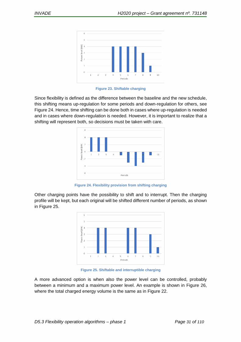
Figure 23. Shiftable charging
Since flexibility is defined as the difference between the baseline and the new schedule,
this shifting means up-regulation for some periods and down-regulation for others, see
Figure 24. Hence, time shifting can be done both in cases where up-regulation is needed
and in cases where down-regulation is needed. However, it is important to realize that a
shifting will represent both, so decisions must be taken with care.
Figure 24. Flexibility provision from shifting charging
Other charging points have the possibility to shift and to interrupt. Then the charging
profile will be kept, but each original will be shifted different number of periods, as shown
in Figure 25.
Figure 25. Shiftable and interruptible charging
A more advanced option is when also the power level can be controlled, probably
between a minimum and a maximum power level. An example is shown in Figure 26,
where the total charged energy volume is the same as in Figure 22.

INVADE H2020 project – Grant agreement nº. 731148
D5.3 Flexibility operation algorithms – phase 1 Page 32 of 110
Figure 26. Controllable power level charging
It should be mentioned that if the IEC 61851-1 standard is followed, every EV can be
controlled. However, not every charge point supports control commands from a platform
nor does every charging point have the ability to locally manage the load of the EV. If we
include the possibility to discharge the battery (V2X), we can control both the charging
and the discharging power levels. An example is given in Figure 27, where a discharging
is performed in periods 3 and 4, while charging is done in all the others. In the end, the
total net energy charged to the battery is equal to the case in Figure 22.
Figure 27. Charging with V2X capabilities
Notice that in the V2X case, the amount of flexibility provided can be high, see Figure
28, which shows the flexibility provided when baseline is according to Figure 22 and
schedule is as presented in Figure 27.
Figure 28. Flexibility provision with V2X capabilities

INVADE H2020 project – Grant agreement nº. 731148
D5.3 Flexibility operation algorithms – phase 1 Page 33 of 110
All the cases illustrated above have the same sum net charging energy. In an operational
setting, the possibility to obtain this is dependent on what information that is available.
Key parameters are:
The connection and disconnection periods
The battery state of charge when connecting, or eventually the charging
demand/preferences
Section 2.6 discusses about EV modelling options depending on available data.
2.5.4 Flexibility from generation units
A generation unit is a technology that produces electricity. In this document, we focus on
local, renewable generation units like wind turbines and solar panels. Which flexibility
options that exist will be dependent on the technology at hand, but basically we divide
into inflexible and curtailable generation units. The latter is again divided into two
groups: disconnectable, i.e. that either must be on or completely off, and reducible,
where the power level can be controlled.
Figure 29. Baseline production for a solar panel
For illustration, assume that a solar panel has a baseline production profile according to
Figure 29. If it is of type curtailable disconnectable, a possible revised profile is shown in
Figure 30, where it is disconnected in period 6 and 7. Hence, the production is 0 in these
periods.
Figure 30. Schedule for disconnectable generation unit
If the solar panel is in the category of curtailable reducible a possible revised profile is
shown in Figure 31, where production is reduced to 2 in the periods 6, 7 and 8.

INVADE H2020 project – Grant agreement nº. 731148
D5.3 Flexibility operation algorithms – phase 1 Page 34 of 110
Figure 31. Schedule for reduceble generation unit
In this document we assume that there are no timing constraints related to when
regulations can be performed, meaning that curtailment can be done at any time and
with any duration. However, constraints can be introduced according to the ones
described under curtailable load units.
Also recall that we only treat wind mills and solar panels in this document. Other
generation technologies like hydro power plants and thermal units, will have different
properties and constraints.
2.5.5 Flexibility from aggregated resources
The cases described in the previous section regarding batteries, EVs, loads and
generation units are explained in case of having information of each single device. For
instance one load appliance or one charging point. In some cases, this might not be the
situation. A typical example is when there are several charging points below one
charging site, and our model is not able to control each of them. Another example is if a
household is modelled as one single resource without having detailed information about
the internal appliances.
In cases where the expected output is an aggregated flexibility curve, some
considerations are necessary.
First of all, in case of having all possible information from flexible assets, the problem
should be handled as previously. Therefore, the aggregated curve from the Integrated
INVADE platform optimization algorithm is composed by all flexible devices and the local
platform can change that scheduling if needed.
2.5.5.1 Flexibility from aggregated resources with partial information at device level
If the information available is just an aggregated curve with different flexibility sources, it
makes flexibility decision problems very complicated as there are no constraints limiting
the feasible flexibility. Therefore, even if the final individual schedule plan is taken by a
local controller or central system, aggregated decision should be taking all devices into
account.
One possibility is that the optimization algorithm suggests a feasible schedule plan at
device level minimizing the cost. Then, the result of this scheduling problem is sent to
the local controller who takes the final decision based on their priorities.

INVADE H2020 project – Grant agreement nº. 731148
D5.3 Flexibility operation algorithms – phase 1 Page 35 of 110
Figure 32. Baseline charging schedule
Figure 33. Optimized and final decision schedules
Notice that both solutions consumes the same energy aggregated but the EV 2 starts
charging at the 5th period instead of 4th period.
2.5.5.2 Flexibility from aggregated resources without information at the device level
In case of not knowing which resources that form the flexibility portfolio, a more generic,
high level model must be defined. One possible approach is to introduce a new resource
type which represents a virtual, flexibility resource.
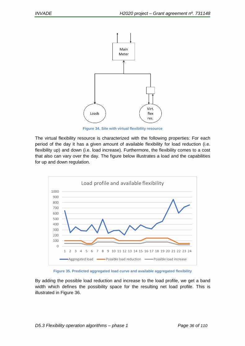
Assume we have a site (a building or a charging site) with an expected load profile. The
site also has a virtual flexibility resource, see illustration in Figure 34.
0
1
2
3
4
5
6
7
1 2 3 4 5 6 7 8
Po
wer
leve
l [kW
]Periods
No flexibility EV1 No flexibility EV2 No flexibility EV3
0
2
4
6
8
1 2 3 4 5 6 7 8Po
wer
leve
l [kW
]
Periods
Optimized plan EV1 Optimized plan EV2
Optimized plan EV3
0
2
4
6
8
1 2 3 4 5 6 7 8Po
wer
leve
l [kW
]
Periods
Final decision EV1 Final decision EV2
Final decision EV3
INVADE H2020 project – Grant agreement nº. 731148
D5.3 Flexibility operation algorithms – phase 1 Page 36 of 110
Figure 34. Site with virtual flexibility resource
The virtual flexibility resource is characterized with the following properties: For each
period of the day it has a given amount of available flexibility for load reduction (i.e.
flexibility up) and down (i.e. load increase). Furthermore, the flexibility comes to a cost
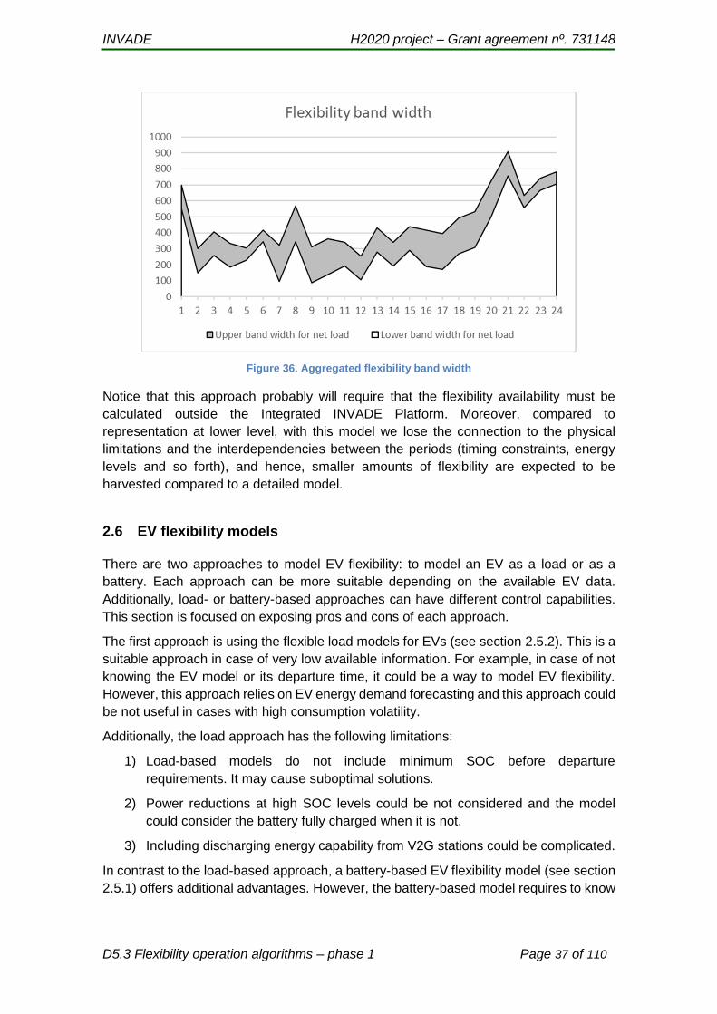
that also can vary over the day. The figure below illustrates a load and the capabilities
for up and down regulation.
Figure 35. Predicted aggregated load curve and available aggregated flexibility
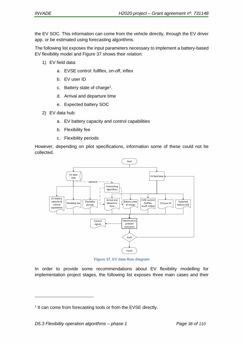
By adding the possible load reduction and increase to the load profile, we get a band
width which defines the possibility space for the resulting net load profile. This is
illustrated in Figure 36.
INVADE H2020 project – Grant agreement nº. 731148
D5.3 Flexibility operation algorithms – phase 1 Page 37 of 110
Figure 36. Aggregated flexibility band width
Notice that this approach probably will require that the flexibility availability must be
calculated outside the Integrated INVADE Platform. Moreover, compared to
representation at lower level, with this model we lose the connection to the physical
limitations and the interdependencies between the periods (timing constraints, energy
levels and so forth), and hence, smaller amounts of flexibility are expected to be
harvested compared to a detailed model.
2.6 EV flexibility models
There are two approaches to model EV flexibility: to model an EV as a load or as a
battery. Each approach can be more suitable depending on the available EV data.
Additionally, load- or battery-based approaches can have different control capabilities.
This section is focused on exposing pros and cons of each approach.
The first approach is using the flexible load models for EVs (see section 2.5.2). This is a
suitable approach in case of very low available information. For example, in case of not
knowing the EV model or its departure time, it could be a way to model EV flexibility.
However, this approach relies on EV energy demand forecasting and this approach could
be not useful in cases with high consumption volatility.
Additionally, the load approach has the following limitations:
1) Load-based models do not include minimum SOC before departure
requirements. It may cause suboptimal solutions.
2) Power reductions at high SOC levels could be not considered and the model
could consider the battery fully charged when it is not.
3) Including discharging energy capability from V2G stations could be complicated.
In contrast to the load-based approach, a battery-based EV flexibility model (see section
2.5.1) offers additional advantages. However, the battery-based model requires to know
INVADE H2020 project – Grant agreement nº. 731148
D5.3 Flexibility operation algorithms – phase 1 Page 38 of 110
the EV SOC. This information can come from the vehicle directly, through the EV driver
app, or be estimated using forecasting algorithms.
The following list exposes the input parameters necessary to implement a battery-based
EV flexibility model and Figure 37 shows their relation:
1) EV field data:
a. EVSE control: fullflex, on-off, inflex
b. EV user ID
c. Battery state of charge1.
d. Arrival and departure time
e. Expected battery SOC
2) EV data hub:
a. EV battery capacity and control capabilities
b. Flexibility fee
c. Flexibility periods
However, depending on pilot specifications, information some of these could not be
collected.
Figure 37. EV data flow diagram
In order to provide some recommendations about EV flexibility modelling for
implementation project stages, the following list exposes three main cases and their
1 It can come from forecasting tools or from the EVSE directly.
EV data Hub
Forecasting algorithms
optional
Arrival and departure
time
Battery state of charge
EVSE control(fullflex,
onoff, inflex)EV/user ID
Optimization problem
execution
End?
Finish
Flexibility fee
EV battery capacity &
control capabilities
Control signals
EV field data
Start
Flexibility periods
Expected battery SOC

INVADE H2020 project – Grant agreement nº. 731148
D5.3 Flexibility operation algorithms – phase 1 Page 39 of 110
modelling options. Depending on available data and the flexibility service, the EV
flexibility modelling can follow one of the following options:
1. In case of having full information, including SOC, and connection/disconnection
times2, the battery-based model is recommended. In this case, the FO can send
control signals to each EV individually or an aggregated value for all charging
points. The second option requires having local intelligence in the charging
station to distribute flexibility between EVs.
2. In contrast, if some information is not known, it is necessary to forecast this data
to estimate the EV flexibility. In this case, EV flexibility can be modelled as a
battery or as a load, depending on the available information.
3. Finally, if the FO does not know which EV is connected to each charging point,
the forecast reliability is much lower than in the second modelling option. If the
energy needs and departure times are quite uncertain, flexibility decisions should
be more conservative. Therefore, the flexibility obtained from an EV could be very
limited. This case can only use load-based models.
Subsections below expose EV flexibility model characteristics in each case. EV model
mathematical formulation is included in section 5.2.3. Sections 5.2.3.5 and 5.2.3.4
describe the battery-based models and their mathematical formulation. The first model
includes V2X capabilities and the second model is a simplified battery model adapted to
EVs.
2.6.1 EV flexibility in households
In case of EV in households, each EV charger will be usually linked to a single EV with
its characteristics and its owner. Households with 2 electric vehicles will most probably
have their corresponding charging points.
The most probable situation in this case is having partial information (the second
modelling option described above), knowing the EV characteristics but without knowing
its SOC or departure time. Therefore, EV flexibility can be modelled as a load or as a
battery, depending on available information.
In case of EV owners highly engaged and willing to share their SOC and departure times,
the EV can be modelled as a battery following the modelling option 1.
2.6.2 EV flexibility in multiple charging points
In cases of multiple charging points within the same installation like office buildings,
shopping centres or similar, the information available can be different and the EV
flexibility model must include their specificities.
2 It includes expected arrival and departure times, in case of EV drivers booking charging stations, and real arrival and departure times coming from the charging station once the driver arrives or leaves.
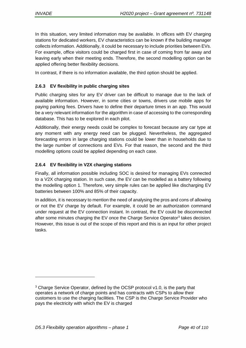
INVADE H2020 project – Grant agreement nº. 731148
D5.3 Flexibility operation algorithms – phase 1 Page 40 of 110
In this situation, very limited information may be available. In offices with EV charging
stations for dedicated workers, EV characteristics can be known if the building manager
collects information. Additionally, it could be necessary to include priorities between EVs.
For example, office visitors could be charged first in case of coming from far away and
leaving early when their meeting ends. Therefore, the second modelling option can be
applied offering better flexibility decisions.
In contrast, if there is no information available, the third option should be applied.
2.6.3 EV flexibility in public charging sites
Public charging sites for any EV driver can be difficult to manage due to the lack of
available information. However, in some cities or towns, drivers use mobile apps for
paying parking fees. Drivers have to define their departure times in an app. This would
be a very relevant information for the algorithm in case of accessing to the corresponding
database. This has to be explored in each pilot.
Additionally, their energy needs could be complex to forecast because any car type at
any moment with any energy need can be plugged. Nevertheless, the aggregated
forecasting errors in large charging stations could be lower than in households due to
the large number of connections and EVs. For that reason, the second and the third
modelling options could be applied depending on each case.
2.6.4 EV flexibility in V2X charging stations
Finally, all information possible including SOC is desired for managing EVs connected
to a V2X charging station. In such case, the EV can be modelled as a battery following
the modelling option 1. Therefore, very simple rules can be applied like discharging EV
batteries between 100% and 85% of their capacity.
In addition, it is necessary to mention the need of analysing the pros and cons of allowing
or not the EV charge by default. For example, it could be an authorization command
under request at the EV connection instant. In contrast, the EV could be disconnected
after some minutes charging the EV once the Charge Service Operator3 takes decision.
However, this issue is out of the scope of this report and this is an input for other project
tasks.
3 Charge Service Operator, defined by the OCSP protocol v1.0, is the party that operates a network of charge points and has contracts with CSPs to allow their customers to use the charging facilities. The CSP is the Charge Service Provider who pays the electricity with which the EV is charged

INVADE H2020 project – Grant agreement nº. 731148
D5.3 Flexibility operation algorithms – phase 1 Page 41 of 110
3 Pilot sites
This chapter describes each of the pilot sites from the perspective of the optimization
model. The description is included here to ensure that the optimization models takes into
account every possible case at the pilot sites. On the other side, this is also about making
the pilots conscious about what they need to discuss and clarify. Since the pilot sites for
the time being are not clearly and in detail defined for all pilots, this chapter will be
updated along with the pilot developments.
3.1 Norway
3.1.1 Introduction
According to D4.2 the focus with the Norwegian pilots will be the Prosumer and the
following flexibility services:
ToU optimization
kWmax control
Self-balancing
There will be three types of Prosumers in the Norwegian pilot:
A number of private households
A number of housing cooperatives
Charging site connected to an office building
3.1.2 Roles and their interrelations
In the Norwegian electricity market, each consumer and prosumer must have two
different contracts: one with the DSO that they are physically connected to and one with
a free of choice retailer. In our context the FO will perform the control actions.
Figure 38. Relations between prosumer, flexibility operator, DSO and Retailer
Notice that the different pilot customers (prosumers) can have different retailers with
different contracts and prices.
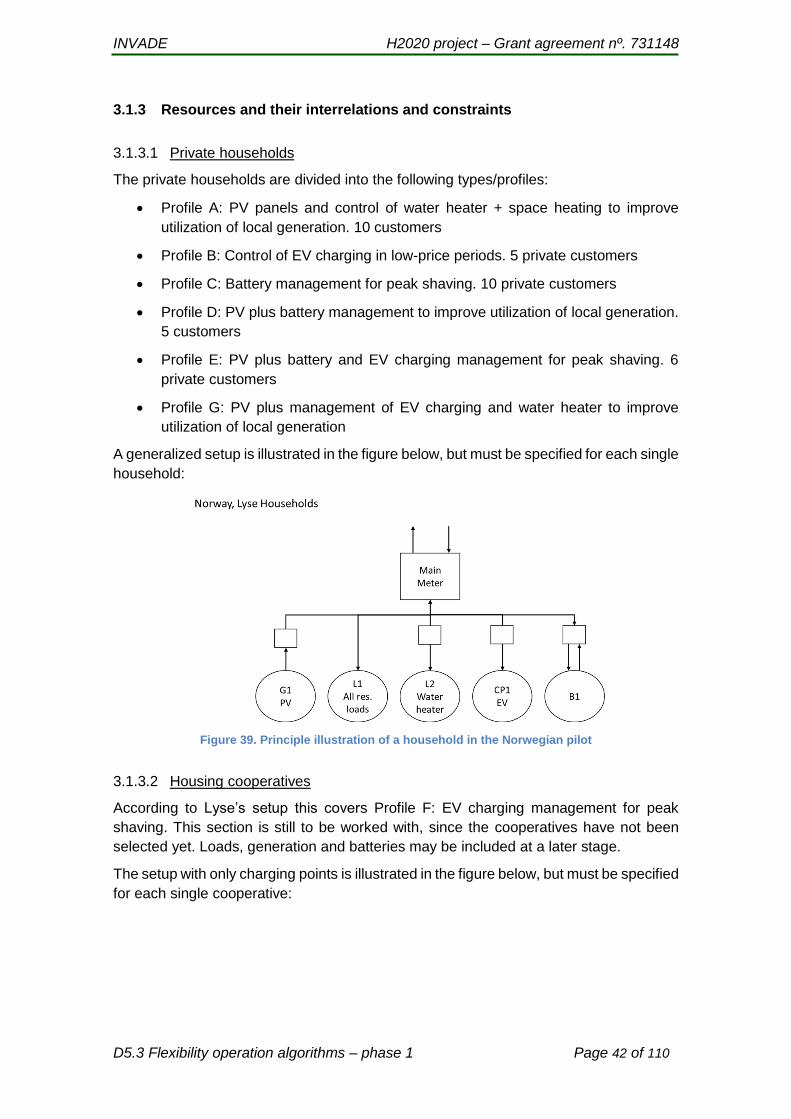
INVADE H2020 project – Grant agreement nº. 731148
D5.3 Flexibility operation algorithms – phase 1 Page 42 of 110
3.1.3 Resources and their interrelations and constraints
3.1.3.1 Private households
The private households are divided into the following types/profiles:
Profile A: PV panels and control of water heater + space heating to improve
utilization of local generation. 10 customers
Profile B: Control of EV charging in low-price periods. 5 private customers
Profile C: Battery management for peak shaving. 10 private customers
Profile D: PV plus battery management to improve utilization of local generation.
5 customers
Profile E: PV plus battery and EV charging management for peak shaving. 6
private customers
Profile G: PV plus management of EV charging and water heater to improve
utilization of local generation
A generalized setup is illustrated in the figure below, but must be specified for each single
household:
Figure 39. Principle illustration of a household in the Norwegian pilot
3.1.3.2 Housing cooperatives
According to Lyse’s setup this covers Profile F: EV charging management for peak
shaving. This section is still to be worked with, since the cooperatives have not been
selected yet. Loads, generation and batteries may be included at a later stage.
The setup with only charging points is illustrated in the figure below, but must be specified
for each single cooperative:
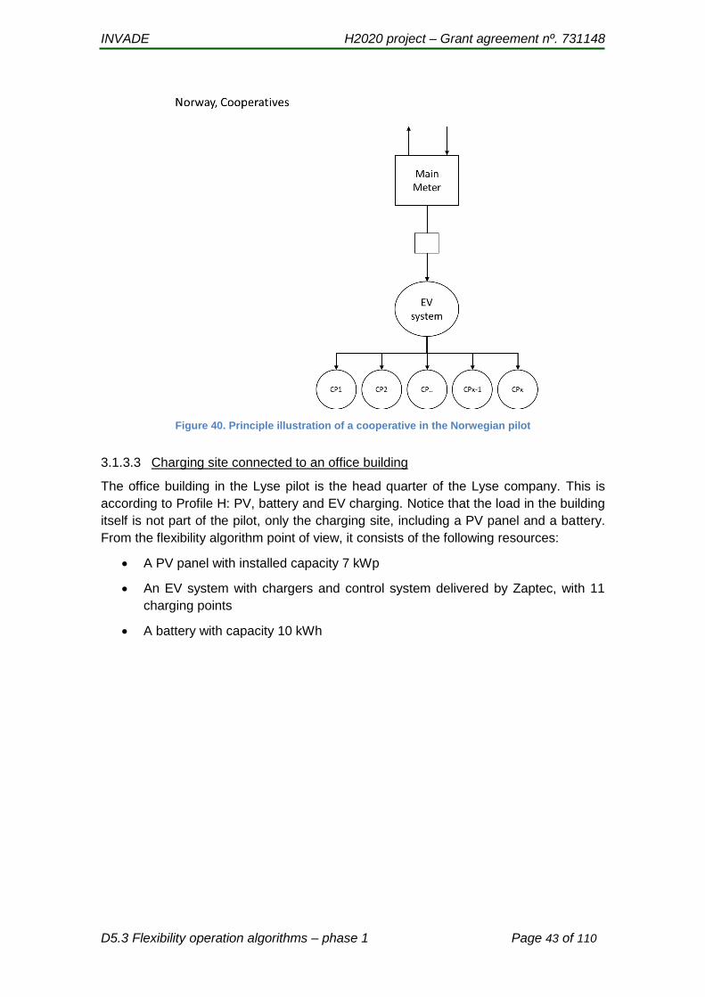
INVADE H2020 project – Grant agreement nº. 731148
D5.3 Flexibility operation algorithms – phase 1 Page 43 of 110
Figure 40. Principle illustration of a cooperative in the Norwegian pilot
3.1.3.3 Charging site connected to an office building
The office building in the Lyse pilot is the head quarter of the Lyse company. This is
according to Profile H: PV, battery and EV charging. Notice that the load in the building
itself is not part of the pilot, only the charging site, including a PV panel and a battery.
From the flexibility algorithm point of view, it consists of the following resources:
A PV panel with installed capacity 7 kWp
An EV system with chargers and control system delivered by Zaptec, with 11
charging points
A battery with capacity 10 kWh
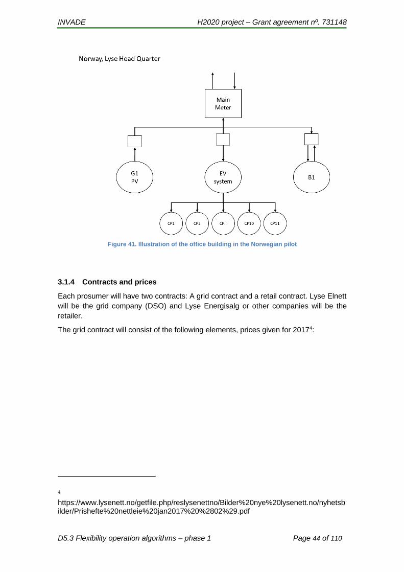
INVADE H2020 project – Grant agreement nº. 731148
D5.3 Flexibility operation algorithms – phase 1 Page 44 of 110
Figure 41. Illustration of the office building in the Norwegian pilot
3.1.4 Contracts and prices
Each prosumer will have two contracts: A grid contract and a retail contract. Lyse Elnett
will be the grid company (DSO) and Lyse Energisalg or other companies will be the
retailer.
The grid contract will consist of the following elements, prices given for 20174:
4 https://www.lysenett.no/getfile.php/reslysenettno/Bilder%20nye%20lysenett.no/nyhetsbilder/Prishefte%20nettleie%20jan2017%20%2802%29.pdf
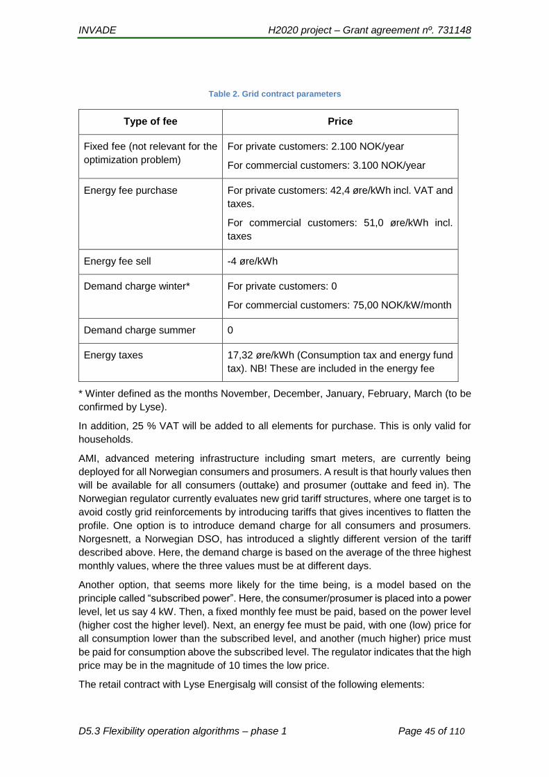
INVADE H2020 project – Grant agreement nº. 731148
D5.3 Flexibility operation algorithms – phase 1 Page 45 of 110
Table 2. Grid contract parameters
Type of fee Price
Fixed fee (not relevant for the
optimization problem)
For private customers: 2.100 NOK/year
For commercial customers: 3.100 NOK/year
Energy fee purchase For private customers: 42,4 øre/kWh incl. VAT and
taxes.
For commercial customers: 51,0 øre/kWh incl.
taxes
Energy fee sell -4 øre/kWh
Demand charge winter* For private customers: 0
For commercial customers: 75,00 NOK/kW/month
Demand charge summer 0
Energy taxes 17,32 øre/kWh (Consumption tax and energy fund
tax). NB! These are included in the energy fee
* Winter defined as the months November, December, January, February, March (to be
confirmed by Lyse).
In addition, 25 % VAT will be added to all elements for purchase. This is only valid for
households.
AMI, advanced metering infrastructure including smart meters, are currently being
deployed for all Norwegian consumers and prosumers. A result is that hourly values then
will be available for all consumers (outtake) and prosumer (outtake and feed in). The
Norwegian regulator currently evaluates new grid tariff structures, where one target is to
avoid costly grid reinforcements by introducing tariffs that gives incentives to flatten the
profile. One option is to introduce demand charge for all consumers and prosumers.
Norgesnett, a Norwegian DSO, has introduced a slightly different version of the tariff
described above. Here, the demand charge is based on the average of the three highest
monthly values, where the three values must be at different days.
Another option, that seems more likely for the time being, is a model based on the
principle called “subscribed power”. Here, the consumer/prosumer is placed into a power
level, let us say 4 kW. Then, a fixed monthly fee must be paid, based on the power level
(higher cost the higher level). Next, an energy fee must be paid, with one (low) price for
all consumption lower than the subscribed level, and another (much higher) price must
be paid for consumption above the subscribed level. The regulator indicates that the high
price may be in the magnitude of 10 times the low price.
The retail contract with Lyse Energisalg will consist of the following elements:

INVADE H2020 project – Grant agreement nº. 731148
D5.3 Flexibility operation algorithms – phase 1 Page 46 of 110
Table 3. Retail contract parameters
Type of fee Price
Fixed fee (not relevant for the
optimization problem)
47 NOK/month
Price for buying For private customers: Elspot price from Nord Pool
Spot for the area NO2/Bergen5 + a mark-up 3,9
øre/kWh
For commercial customers: Elspot price from Nord
Pool Spot for the area NO2/Bergen + a mark-up
4,6 øre/kWh
Price for selling 2*Elspot price from Nord Pool Spot, see price for
buying6
For other retailers, the contracts will be different. The model must cover different types,
for instance fixed prices for longer time intervals and other types where the price varies
according to Elspot price, but with other mark-ups.
For prosumers, the sales of surplus electricity is regulated through the retail contract.
Also here, different models exist. The most usual model currently, is that the surplus
electricity is compensated with the same price as the deficit. In other words, the buying
and selling price are the same. However, it must be commented that although the retail
prices are equal, the cost of one kWh used is much higher than the revenue from one
kWh sold. The reason for this is the grid tariff and the taxes.
In order to make it easier for consumers to turn into prosumers, the Norwegian regulator
has introduced what they call the “plus-customer arrangement”. Traditionally, a
consumer must enter an agreement with the DSO for outtake, while a producer must
enter an agreement for feed in. Through the plus-customer arrangement the prosumer
can only have one agreement. However, a prerequisite for participating in this
arrangement is that the net feed in never is more than 100 kWh/h. For small prosumers,
this is not a problem, but for larger buildings and industries it might be a challenge.
Flexibility, for instance represented by batteries, may then be used to avoid breaking this
constraint.
5 http://nordpoolspot.com/historical-market-data/
6 https://sol.lyse.no/stromavtale/
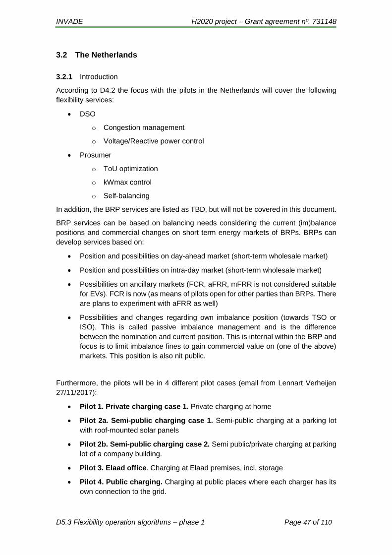
INVADE H2020 project – Grant agreement nº. 731148
D5.3 Flexibility operation algorithms – phase 1 Page 47 of 110
3.2 The Netherlands
3.2.1 Introduction
According to D4.2 the focus with the pilots in the Netherlands will cover the following
flexibility services:
DSO
o Congestion management
o Voltage/Reactive power control
Prosumer
o ToU optimization
o kWmax control
o Self-balancing
In addition, the BRP services are listed as TBD, but will not be covered in this document.
BRP services can be based on balancing needs considering the current (im)balance
positions and commercial changes on short term energy markets of BRPs. BRPs can
develop services based on:
Position and possibilities on day-ahead market (short-term wholesale market)
Position and possibilities on intra-day market (short-term wholesale market)
Possibilities on ancillary markets (FCR, aFRR, mFRR is not considered suitable
for EVs). FCR is now (as means of pilots open for other parties than BRPs. There
are plans to experiment with aFRR as well)
Possibilities and changes regarding own imbalance position (towards TSO or
ISO). This is called passive imbalance management and is the difference
between the nomination and current position. This is internal within the BRP and
focus is to limit imbalance fines to gain commercial value on (one of the above)
markets. This position is also nit public.
Furthermore, the pilots will be in 4 different pilot cases (email from Lennart Verheijen
27/11/2017):
Pilot 1. Private charging case 1. Private charging at home
Pilot 2a. Semi-public charging case 1. Semi-public charging at a parking lot
with roof-mounted solar panels
Pilot 2b. Semi-public charging case 2. Semi public/private charging at parking
lot of a company building.
Pilot 3. Elaad office. Charging at Elaad premises, incl. storage
Pilot 4. Public charging. Charging at public places where each charger has its
own connection to the grid.
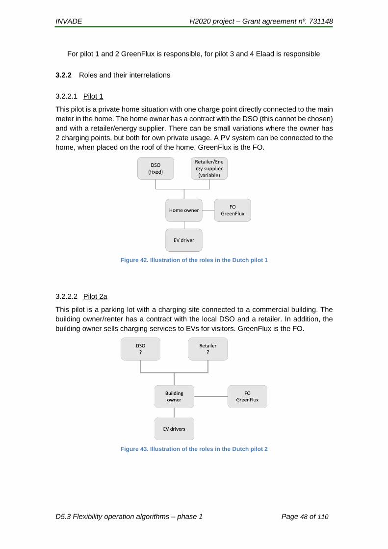
INVADE H2020 project – Grant agreement nº. 731148
D5.3 Flexibility operation algorithms – phase 1 Page 48 of 110
For pilot 1 and 2 GreenFlux is responsible, for pilot 3 and 4 Elaad is responsible
3.2.2 Roles and their interrelations
3.2.2.1 Pilot 1
This pilot is a private home situation with one charge point directly connected to the main
meter in the home. The home owner has a contract with the DSO (this cannot be chosen)
and with a retailer/energy supplier. There can be small variations where the owner has
2 charging points, but both for own private usage. A PV system can be connected to the
home, when placed on the roof of the home. GreenFlux is the FO.
Figure 42. Illustration of the roles in the Dutch pilot 1
3.2.2.2 Pilot 2a
This pilot is a parking lot with a charging site connected to a commercial building. The
building owner/renter has a contract with the local DSO and a retailer. In addition, the
building owner sells charging services to EVs for visitors. GreenFlux is the FO.
Figure 43. Illustration of the roles in the Dutch pilot 2

INVADE H2020 project – Grant agreement nº. 731148
D5.3 Flexibility operation algorithms – phase 1 Page 49 of 110
3.2.2.3 Pilot 2b
In this pilot GreenFlux will be the FO that controls the charging below specified limits. No
other roles are involved.
3.2.2.4 Pilot 3: Small scale office
Figure 44. Pilot 3
At this pilot site we consider 3 optimization levels:
Locally behind the connection point (done by CPMS Elaad). We will construct the system / architecture that we can work here with different (optimization) algorithms.
Locally in agreement with the local DSO. DSO contracts flexibility for local congestion challenges (done by us and the resp. DSO first based on meter values in later stage based on de facto standard OSCP)
National level; flexibility is provided to BRP (portfolio-optimization) and TSO (frequency mgt , ancillary markets) and higher level (MV) DSO grids (congestion); (this we can provide to eSmart / Invade platform)
We can offer from the large scale office site an aggregated profile of tomorrows load with
bandwidths, an aggregated forecast which is already locally optimised. The bandwith
consists of the (expected) flexibilities of the ev-drivers+the storage unit+building. Local
optimisation first, then local congestion mgt to local DSO. Then the flex which is left is
sent to the aggregated platform.
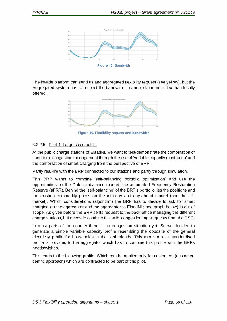
INVADE H2020 project – Grant agreement nº. 731148
D5.3 Flexibility operation algorithms – phase 1 Page 50 of 110
Figure 45. Bandwith
The invade platform can send us and aggregated flexibility request (see yellow), but the
Aggregated system has to respect the bandwith. It cannot claim more flex than locally
offered.
Figure 46. Flexibility request and bandwidth
3.2.2.5 Pilot 4: Large scale public
At the public charge stations of ElaadNL we want to test/demonstrate the combination of
short term congestion management through the use of ‘variable capacity (contracts)’ and
the combination of smart charging from the perspective of BRP.
Partly real-life with the BRP connected to our stations and partly through simulation.
This BRP wants to combine ‘self-balancing portfolio optimization’ and use the
opportunities on the Dutch imbalance market, the automated Frequency Restoration
Reserve (aFRR). Behind the ‘self-balancing’ of the BRP’s portfolio lies the positions and
the existing commodity prices on the intraday and day-ahead market (and the LT-
market). Which considerations (algorithm) the BRP has to decide to ask for smart
charging (to the aggregator and the aggregator to ElaadNL; see graph below) is out of
scope. As given before the BRP sents request to the back-office managing the different
charge stations, but needs to combine this with ‘congestion mgt-requests from the DSO.
In most parts of the country there is no congestion situation yet. So we decided to
generate a simple variable capacity profile resembling the opposite of the general
electricity profile for households in the Netherlands. This more or less standardised
profile is provided to the aggregator which has to combine this profile with the BRPs
needs/wishes.
This leads to the following profile. Which can be applied only for customers (customer-
centric approach) which are contracted to be part of this pilot.
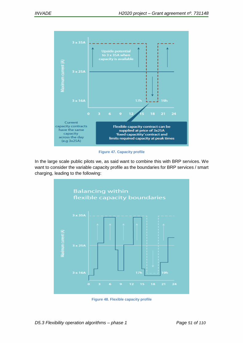
INVADE H2020 project – Grant agreement nº. 731148
D5.3 Flexibility operation algorithms – phase 1 Page 51 of 110
Figure 47. Capacity profile
In the large scale public pilots we, as said want to combine this with BRP services. We
want to consider the variable capacity profile as the boundaries for BRP services / smart
charging, leading to the following:
Figure 48. Flexible capacity profile

INVADE H2020 project – Grant agreement nº. 731148
D5.3 Flexibility operation algorithms – phase 1 Page 52 of 110
Stations in the field are single or duo-socket stations all managed by ElaadNL. Grid
connection is 3x25A or 3x35A. the ElaadNL system will receive input from BRP and
effectuates the charging profile within the given DSO limits.
3.2.3 Resources and their interrelations and constraints
3.2.3.1 Pilot 1
In this case a home has 1 private charge point. The charge point is connected to the
main meter in the home, however for monitoring and control issues, each station has its
own meter as well and is connected to a charge point management system. The home
is using an average consumption of 4000 kW per year. The charge point can deliver max
11kW. In the situations where PV is available on the roof of the homes, it delivers
on2000kW per year on average.
The purpose of smart charging is to optimize the business case for the combination of
the PV-system and the EV charger. The secondary goal is to charge the EV as fast as
possible. This means that:
The EV will increase its charge rate if the real time solar production increases
The EV will decrease its charge if:
o The real time solar production decreases
o The other consumption in the household significantly increases. The total
grid connection of the household is 3x25A, this should never be
overloaded7.
Figure 49. Illustration of pilot 1 in the Dutch pilot
7 Theoretically it is possible to charge at higher rates than 3x25A with the EV. E.g. if the household consumes nothing and the solar panels produce 3x10A, then the EV could charge at 3x35A. This is however not allowed by the Dutch grid operator. Maximum charging speed of the EV may never be higher than the grid connection: 3x25A.
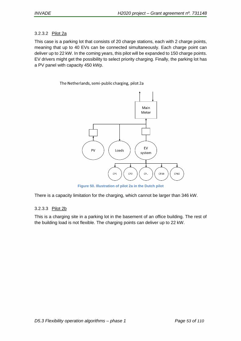
INVADE H2020 project – Grant agreement nº. 731148
D5.3 Flexibility operation algorithms – phase 1 Page 53 of 110
3.2.3.2 Pilot 2a
This case is a parking lot that consists of 20 charge stations, each with 2 charge points,
meaning that up to 40 EVs can be connected simultaneously. Each charge point can
deliver up to 22 kW. In the coming years, this pilot will be expanded to 150 charge points.
EV drivers might get the possibility to select priority charging. Finally, the parking lot has
a PV panel with capacity 450 kWp.
Figure 50. Illustration of pilot 2a in the Dutch pilot
There is a capacity limitation for the charging, which cannot be larger than 346 kW.
3.2.3.3 Pilot 2b
This is a charging site in a parking lot in the basement of an office building. The rest of
the building load is not flexible. The charging points can deliver up to 22 kW.

INVADE H2020 project – Grant agreement nº. 731148
D5.3 Flexibility operation algorithms – phase 1 Page 54 of 110
Figure 51. Illustration of pilot 2b in the Dutch pilot
There are two levels of capacity limitation:
Each of the three charging point groups must be below 173 kW
The total consumption (building load + EV) must be below 436 kW
3.2.3.4 Small scale office
This site was recently extracted. The following situation exists.

INVADE H2020 project – Grant agreement nº. 731148
D5.3 Flexibility operation algorithms – phase 1 Page 55 of 110
Figure 52. Small scale office
Numbers 1 - 19: charging stations (single or dual socket) Number 20: dc charging station Numbers 21 - 22: locations for experimental charging stations Number 23: charging site
At the site there is installed
4 kWp solar system Local server and network (that communicate with cloud services and can
perform smart charging based on different optimization algorithms)
The ‘technical situation’ is:
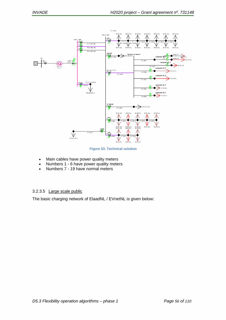
INVADE H2020 project – Grant agreement nº. 731148
D5.3 Flexibility operation algorithms – phase 1 Page 56 of 110
Figure 53. Technical solution
Main cables have power quality meters Numbers 1 - 6 have power quality meters Numbers 7 - 19 have normal meters
3.2.3.5 Large scale public
The basic charging network of ElaadNL / EVnetNL is given below:
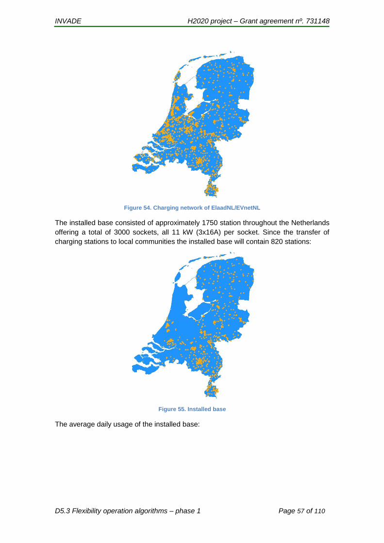
INVADE H2020 project – Grant agreement nº. 731148
D5.3 Flexibility operation algorithms – phase 1 Page 57 of 110
Figure 54. Charging network of ElaadNL/EVnetNL
The installed base consisted of approximately 1750 station throughout the Netherlands
offering a total of 3000 sockets, all 11 kW (3x16A) per socket. Since the transfer of
charging stations to local communities the installed base will contain 820 stations:
Figure 55. Installed base
The average daily usage of the installed base:

INVADE H2020 project – Grant agreement nº. 731148
D5.3 Flexibility operation algorithms – phase 1 Page 58 of 110
Figure 56. Daily average use of the installed base
The percentage of charging sessions is given below. The graph shows the hour within
the charging session is started. This graph (although consisting of averages) shows the
fact that EV charging is increasing the already existing peak demand at peak times.
Figure 57. Percentage of charging sessions starting up

INVADE H2020 project – Grant agreement nº. 731148
D5.3 Flexibility operation algorithms – phase 1 Page 59 of 110
At the same time, we see that there is quite a lot of flexibility present during the charge
sessions. When we compare the ‘connection time’ with the ‘charging time’ we get the
following result;
Figure 58. Flexibility from charge sessions
We see a lot of flexibility potential at the evening and night.
3.2.4 Contracts and prices
3.2.4.1 Pilot 1
There are two contracts that are involved in this pilot: The grid contract and the
supply/retail contract.
The grid contract is based on a peak demand charge for the year. This means that it is
an incentive to reduce this peak (hourly value) as much as possible.
The supply contract for buying electricity is normally an average fixed price for a full
period (1 or 2 years). This pilot is using contract where energy retail prices are based on
hourly prices at EPEX Spot8 without any mark-up or other fees that are relevant for the
flexibility algorithm. This contract also regulates the price for sales of surplus electricity
sales. This price is 0,18 €/kWh on average. The price change per hour. The home owner
pays the average price and get a refund or surplus at the end of a period depending on
the real prices and usage.
8 https://www.apxgroup.com/market-results/apx-power-nl/dashboard/
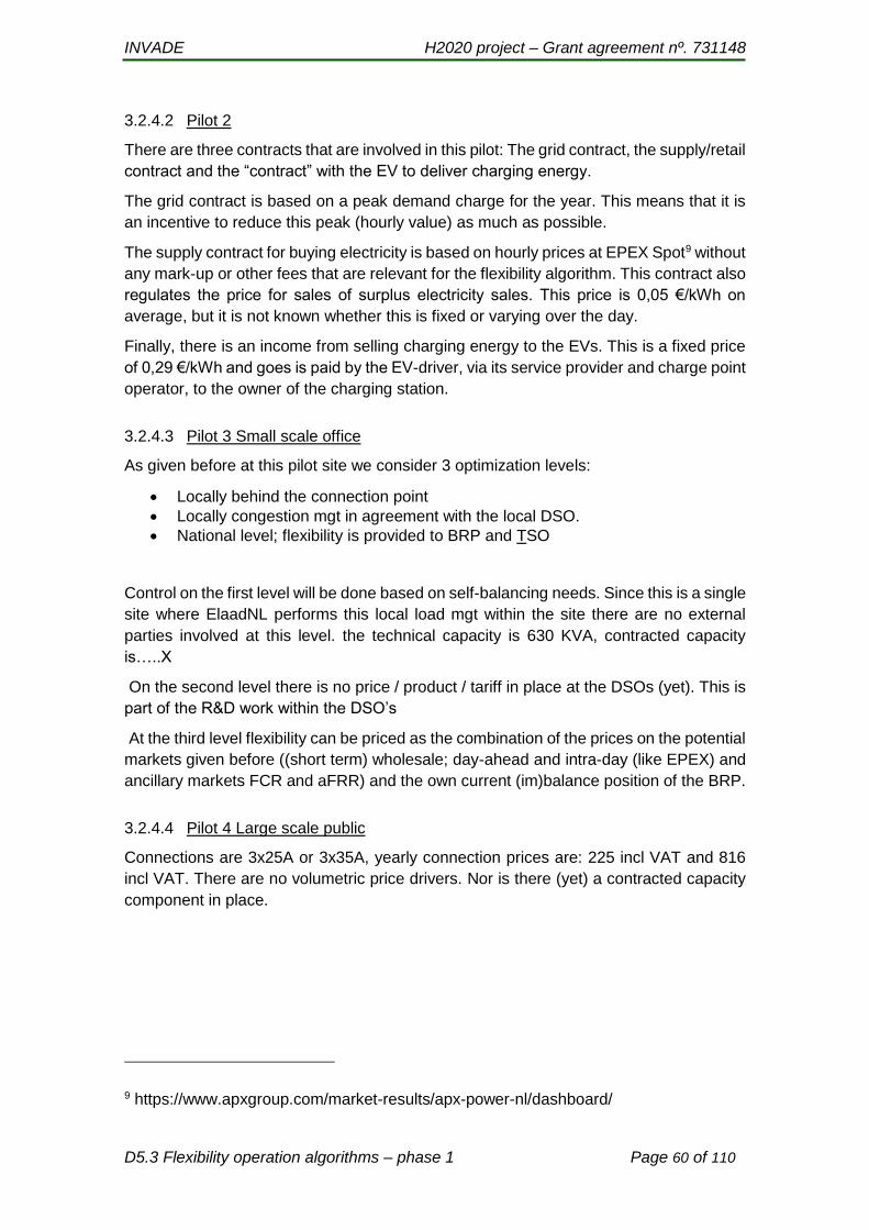
INVADE H2020 project – Grant agreement nº. 731148
D5.3 Flexibility operation algorithms – phase 1 Page 60 of 110
3.2.4.2 Pilot 2
There are three contracts that are involved in this pilot: The grid contract, the supply/retail
contract and the “contract” with the EV to deliver charging energy.
The grid contract is based on a peak demand charge for the year. This means that it is
an incentive to reduce this peak (hourly value) as much as possible.
The supply contract for buying electricity is based on hourly prices at EPEX Spot9 without
any mark-up or other fees that are relevant for the flexibility algorithm. This contract also
regulates the price for sales of surplus electricity sales. This price is 0,05 €/kWh on
average, but it is not known whether this is fixed or varying over the day.
Finally, there is an income from selling charging energy to the EVs. This is a fixed price
of 0,29 €/kWh and goes is paid by the EV-driver, via its service provider and charge point
operator, to the owner of the charging station.
3.2.4.3 Pilot 3 Small scale office
As given before at this pilot site we consider 3 optimization levels:
Locally behind the connection point
Locally congestion mgt in agreement with the local DSO.
National level; flexibility is provided to BRP and TSO
Control on the first level will be done based on self-balancing needs. Since this is a single
site where ElaadNL performs this local load mgt within the site there are no external
parties involved at this level. the technical capacity is 630 KVA, contracted capacity
is…..X
On the second level there is no price / product / tariff in place at the DSOs (yet). This is
part of the R&D work within the DSO’s
At the third level flexibility can be priced as the combination of the prices on the potential
markets given before ((short term) wholesale; day-ahead and intra-day (like EPEX) and
ancillary markets FCR and aFRR) and the own current (im)balance position of the BRP.
3.2.4.4 Pilot 4 Large scale public
Connections are 3x25A or 3x35A, yearly connection prices are: 225 incl VAT and 816
incl VAT. There are no volumetric price drivers. Nor is there (yet) a contracted capacity
component in place.
9 https://www.apxgroup.com/market-results/apx-power-nl/dashboard/
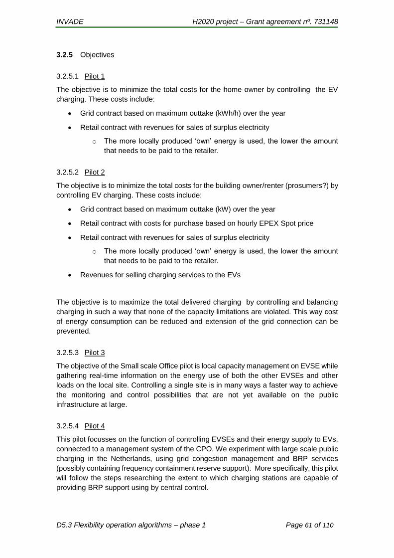
INVADE H2020 project – Grant agreement nº. 731148
D5.3 Flexibility operation algorithms – phase 1 Page 61 of 110
3.2.5 Objectives
3.2.5.1 Pilot 1
The objective is to minimize the total costs for the home owner by controlling the EV
charging. These costs include:
Grid contract based on maximum outtake (kWh/h) over the year
Retail contract with revenues for sales of surplus electricity
o The more locally produced ‘own’ energy is used, the lower the amount
that needs to be paid to the retailer.
3.2.5.2 Pilot 2
The objective is to minimize the total costs for the building owner/renter (prosumers?) by
controlling EV charging. These costs include:
Grid contract based on maximum outtake (kW) over the year
Retail contract with costs for purchase based on hourly EPEX Spot price
Retail contract with revenues for sales of surplus electricity
o The more locally produced ‘own’ energy is used, the lower the amount
that needs to be paid to the retailer.
Revenues for selling charging services to the EVs
The objective is to maximize the total delivered charging by controlling and balancing
charging in such a way that none of the capacity limitations are violated. This way cost
of energy consumption can be reduced and extension of the grid connection can be
prevented.
3.2.5.3 Pilot 3
The objective of the Small scale Office pilot is local capacity management on EVSE while
gathering real-time information on the energy use of both the other EVSEs and other
loads on the local site. Controlling a single site is in many ways a faster way to achieve
the monitoring and control possibilities that are not yet available on the public
infrastructure at large.
3.2.5.4 Pilot 4
This pilot focusses on the function of controlling EVSEs and their energy supply to EVs,
connected to a management system of the CPO. We experiment with large scale public
charging in the Netherlands, using grid congestion management and BRP services
(possibly containing frequency containment reserve support). More specifically, this pilot
will follow the steps researching the extent to which charging stations are capable of
providing BRP support using by central control.

INVADE H2020 project – Grant agreement nº. 731148
D5.3 Flexibility operation algorithms – phase 1 Page 62 of 110
Current pricing regime is based on flat, fixed prices dependent on fuse size (grid
contract?). However, new tariff regimes will be tested in the project.
A new grid tariff type is the “Dynamic capacity” which works like this:
The customer has a given main fuse size, e.g. 3X35 A. Normal tariff rate is a fixed
fee, e.g. 800 €/year
If the customer can guarantee that he/she will not surge above 3X25 A in certain
peak hours, he/she will pay a reduced rate, e.g. 200 €/year. Which hour that are
included in the definition of peak hours are dynamic, but will be known in advance
Figure 59 illustrates the principle. Here, up to 24 kW can be bought in the non-peak hours
defined by the hours 8 – 10 and 17 – 21. For the peak hours 8 – 10 and 17 – 21, the
capacity is reduced to 17 kW.
Figure 59. Illustration of the tariff type “Dynamic capacity”
A central question to clarify is what happens if the customer goes above the capacity
limit for the peak hours:
Black-out?
It is allowed, but then the higher fee must be paid?
It is allowed, but only a limited number of times each month/week
Another question is whether the limit is instant (kW) or per hour (kWh/h)?
3.3 Spain
3.3.1 Introduction
According to D4.2, the focus in the Spanish pilot will be the following flexibility services
to the DSO and BRP:
DSO:

INVADE H2020 project – Grant agreement nº. 731148
D5.3 Flexibility operation algorithms – phase 1 Page 63 of 110
o Congestion management
o Voltage / Reactive power control
o Controlled islanding
BRP:
o Intraday portfolio optimization
o Self-balancing portfolio optimization
Services to the BRP will be developed in the second implementation phase of the project,
so they are not covered in this document and will be described in D5.4. In addition,
services for prosumers will not be tested in this pilot.
There will be one pilot site, consisting of one secondary substation and its area of
influence, which includes the EPESA headquarter.
3.3.2 Roles and their interrelations
The FO role is played in this pilot by the retailer company Mercator, which is also owned
by EPESA. Flexibility is obtained from the centralized battery owned by Mercator and it
is used to offer services to the DSO (EPESA) and the BRP/retailer (Mercator). As it can
be seen in Figure 60, some of the different roles will be played by the same actor. In
addition, EPESA is one among the prosumers inside the area of influence of the affected
secondary substation, so it will be also benefited by the controlled islanding service.
Figure 60. Relations between prosumer, flexibility operator, DSO and Retailer/BRP
3.3.3 Resources and their interrelations and constraints
According to the pilot proposal, the pilot consists on a unique centralized battery with a
capacity of 200 kWh and a limited charge and discharge power of 100 kVA. It can be
connected in one of the following parts of the low voltage grid: at the low voltage bus
between the transformer and the low voltage cabinet, at the low voltage cabinet on the
consumption side, or in an intermediate point of the low voltage grid. The final decision
will depend on the preference of the electrical department inside the DSO.
Part of the battery capacity has to be reserved to provide supply to the controlled
islanding. The rest of the capacity can then be used to provide other services to the DSO
and BRP indistinctly.
Flex.
€
Flex.
€
Flex. €
Retailer/BRPMercator
FOMercator
DSOEPESA
Centralized batteryMercator
Flexibility exchanged Flexibility billing
INVADE H2020 project – Grant agreement nº. 731148
D5.3 Flexibility operation algorithms – phase 1 Page 64 of 110
The battery will have a smart meter to monitor and invoice its energy exchanges with the
grid. The control capabilities will be fully integrated into the SCADA and the distribution
management system.
3.3.4 Contracts and prices
According to the current regulation applied in Spain, the battery cannot be considered
as a generator, so its discharges cannot be reimbursed and only its charges will be
invoiced.
Regarding the invoice of energy, the electric tariff present in the Spanish pilot includes
two main components, a per kW charge (contracted power) and a per kWh charge
(energy consumption). It has the following general structure:
𝐸𝑙𝑒𝑐𝑡𝑟𝑖𝑐 𝐵𝑖𝑙𝑙 = [(𝜒𝑦,𝑡,𝑠𝑔𝑟𝑖𝑑−𝑖𝑚𝑝𝑜𝑟𝑡
× 𝑃𝑦,𝑡,𝑠𝑔𝑟𝑖𝑑−𝑖𝑚𝑝𝑜𝑟𝑡
+ 𝐶𝑃 × 𝑃𝑇 × 𝑇𝑖𝑚𝑒) × 𝑇𝑜𝐸 + 𝑅𝐸𝑀 × 𝑇𝑖𝑚𝑒] × 𝑉𝐴𝑇
where:
Energy term (𝑃𝑦,𝑡,𝑠𝑔𝑟𝑖𝑑−𝑖𝑚𝑝𝑜𝑟𝑡
): it multiplies the energy consumption (𝜒𝑦,𝑡,𝑠𝑔𝑟𝑖𝑑−𝑖𝑚𝑝𝑜𝑟𝑡
)
recorded between the dates of the reading for the price of kWh.
Power term (PT): it multiplies the contracted power (CP) by actual days of billing
and the unit price for kW. The contracted power is a fixed value and can be only
changed once a year. In households, if this power is exceed, the smart meter cuts
the supply and it needs to be rearmed manually.
Tax on electricity (ToE): it is a tax regulated by the National Tax Agency. It is
calculated by multiplying the sum of the terms of power and energy by a fixed
amount of 1.0511269.
Rental of equipment of measure (REM): price that the DSO charges if the client
does not own the meter (which is usually the most common case).
VAT quota: application of the percentage of current VAT (21%).
In addition, tariffs can have several periods with different energy prices. In bigger
consumers (>15 kW), there is a penalization if the monthly maximum power exceeds
105% of the CP, and a discount of 15% is applied if the monthly maximum power is
below 85% of the CP. In addition, customers pay a significant penalty each month if their
PF is below 0.95. Available tariffs for CP>15kW are:
3.0 A with 3 energy time periods and 3 power time periods. This tariff has three
periods. These periods are peak (P1), shoulder (P2) and off-peak (P3), in which
shoulder rates usually apply in between peak and off-peak periods.
Table 4 shows the schedule of the time periods for the 3.0 A tariff, and Table 5 gives an
example of yearly-fixed rates for the tariff 3.0A with more than 15 kW contracted power
offered by Mercator.

INVADE H2020 project – Grant agreement nº. 731148
D5.3 Flexibility operation algorithms – phase 1 Page 65 of 110
Table 4. Schedule of the time periods of 3.0 A tariff.
Tariff name
Periods Winter Summer
3.0A (CP>15
kW)
P1 (Peak) 12h to 15h 19h to 22h
P2 (shoulder) 9h to 18h and
23h to 24h 9h to 11h and
16h to 24h
P3 (Off-peak) 0h to 8h 0h to 8h
Table 5. Example of yearly-fixed rates for 3.0 A tariffs10.
Tariff name
Periods Power term (PT) Energy term
(𝑃𝑦,𝑡,𝑠𝑔𝑟𝑖𝑑−𝑖𝑚𝑝𝑜𝑟𝑡
)
3.0A (CP>15
kW)
P1 (Peak) 0,113818 €/kW/day 0,115625 €/kWh
P2 (shoulder) 0,068291 €/kW/day 0,099795 €/kWh
P3 (Off-peak) 0,045527 €/kW/day 0,071165 €/kWh
3.3.5 Objective
The flexibility for the DSO in the Spanish pilot will be used for multiple purposes: island
creation and to reduce the medium voltage grid congestions. A combination of the
following actions will be utilized to obtain these objectives:
To charge or discharge the battery during congestion hours according to DSO
requests.
To ensure that enough capacity is available in the battery to provide these services
to the DSO, prioritizing the charge of the battery during off-peak hours and the
discharge the battery during peak periods.
3.4 Germany
Since the German pilot is not completely defined yet, it is left out in this document.
10 Tariffs given for 2017. www.estabanell.cat/serveis/tarifes
INVADE H2020 project – Grant agreement nº. 731148
D5.3 Flexibility operation algorithms – phase 1 Page 66 of 110
4 Uncertainty, information structure and the planning
process
4.1 Problem description
Optimized operational scheduling of different types loads (shiftable, controllable and
curtailable) and battery charging / discharging with the maximum utilization of RES
generation is the key for providing flexibility services. The optimization process uses the
models of the generation, storage and load units and the other input parameters to
produce the best possible operation schedules of the units for future periods. At the time
of scheduling of the operation, many of the input parameters are not known certainly.
The accuracy of these input parameters decide the quality of the flexibility services. The
optimization process can show significant sensitivity to the uncertainties in the input
parameters, and produces suboptimal solution or even end up in infeasible solution.
Thus, the process of optimization becomes potentially worthless [1].
The dependency of the input parameter and the impact due to their uncertainty varies
for different services defined in the INVADE as per D4.2.
Some of the examples of uncertain input parameters are listed below
1. Total solar energy production from PV units and their power generation at every
instant or in a time period.
2. Energy consumption of different load units, their load profile and time of operation.
3. EV charging consumption, their availability for charging, arrival and departure time.
4. Energy prices at different hours of the day.
5. The time of service request from the DSO to provide flexibility service, start time of
service delivery and duration of service.
The different optimization methods handle these uncertainties with different approaches.
They have their own advantages and disadvantages in terms of computational time,
degree of closeness to the global optimal values and the level of complexity to implement
as an automatic software service.
Further sections in this chapter will detail the uncertainties associated with different input
parameters, the different methods followed to produce optimum operational scheduling
under such circumstances, information structure for handing input parameters to produce
scheduling decisions, the planning time horizon for their effective utilization and the time
resolution of the control actions. Finally, an overview of the operational scheduling
optimization process is presented.
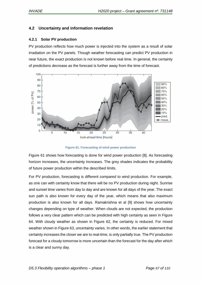
INVADE H2020 project – Grant agreement nº. 731148
D5.3 Flexibility operation algorithms – phase 1 Page 67 of 110
4.2 Uncertainty and information revelation
4.2.1 Solar PV production
PV production reflects how much power is injected into the system as a result of solar
irradiation on the PV panels. Though weather forecasting can predict PV production in
near future, the exact production is not known before real time. In general, the certainty
of predictions decrease as the forecast is further away from the time of forecast.
Figure 61. Forecasting of wind power production
Figure 61 shows how forecasting is done for wind power production [8]. As forecasting
horizon increases, the uncertainty increases. The grey shades indicates the probability
of future power production within the described limits.
For PV production, forecasting is different compared to wind production. For example,
as one can with certainty know that there will be no PV production during night. Sunrise
and sunset time varies from day to day and are known for all days of the year. The exact
sun path is also known for every day of the year, which means that also maximum
production is also known for all days. Ramakrishna et al [9] shows how uncertainty
changes depending on type of weather. When clouds are not expected, the production
follows a very clear pattern which can be predicted with high certainty as seen in Figure
64. With cloudy weather as shown in Figure 62, the certainty is reduced. For mixed
weather shown in Figure 63, uncertainty varies. In other words, the earlier statement that
certainty increases the closer we are to real-time, is only partially true. The PV production
forecast for a cloudy tomorrow is more uncertain than the forecast for the day after which
is a clear and sunny day.
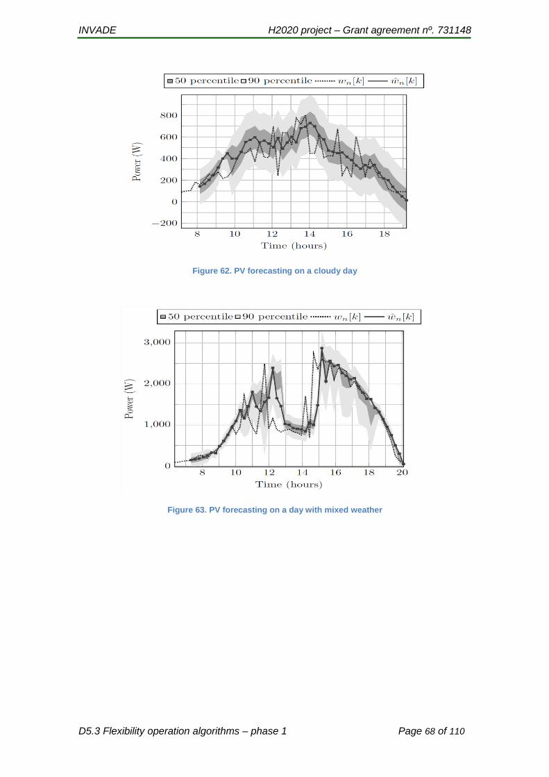
INVADE H2020 project – Grant agreement nº. 731148
D5.3 Flexibility operation algorithms – phase 1 Page 68 of 110
Figure 62. PV forecasting on a cloudy day
Figure 63. PV forecasting on a day with mixed weather

INVADE H2020 project – Grant agreement nº. 731148
D5.3 Flexibility operation algorithms – phase 1 Page 69 of 110
Figure 64. PV forecasting on a sunny day.
4.2.2 Consumption at load limits
Load unit consumption uncertainty differs greatly from device to device. Some load units
like freezers have a fairly predictable load consumption as they are rarely opened, are
well isolated and are in a constant ambient temperature location. Other load units are
less predictable and can only be predicted with very high uncertainty such as water
boilers or TVs.
Load predictions can be made for the future, but certainty does not necessarily increase
greatly the closer to the presence the forecast time horizon is. Some things are known:
The load will be between 0 and the installed capacity of the electrical device
Devices have different characteristics
o Some devices are either on or off
Water heaters, water boilers, lights (mostly), TVs
o Some devices can be configured to different power levels
Heat pumps, stoves
Depending on type of load, it is possible to make some predictions. The possible time of
operation of those loads that are used when people are home are forecasted to get
activate at hours when the resident is at home. If we assume a normal working schedule,
appliances such as stoves, TVs, lights and speakers can be assumed to mainly be used
from 4 pm until midnight and from 6 am to 9 am in the morning. In other words, there is
high certainty in the load forecast from midnight to 6 am and from 9 am to 4 pm compared

INVADE H2020 project – Grant agreement nº. 731148
D5.3 Flexibility operation algorithms – phase 1 Page 70 of 110
to the other hours of a day. The certainty of these loads prediction is close to 100% at 4
am every day of the year, but can only be predicted with lower certainty at 8 pm. In other
words, uncertainty does not necessarily increase the close to real-time we get for these
loads. However, the historical data can reveal consumer behaviour patterns which can
be used to make decent predictions.
Space heating loads normally correlate well with ambient temperature, and can therefore
be forecasted fairly well. However, uncertainty varies depending on what kind of heating
device it is. Some heating devices switch ON and OFF and are automatically regulated
by a control device which has a temperature sensor. This means that by knowing ambient
temperature, consumption over a longer time period (e.g. 24 hours) can be predicted
with low uncertainty, compared to the prediction of their real-time duty cycle. Other space
heating devices are not automatically regulated, but are controlled by end users
manually.
4.2.3 Aggregated consumption of load units
Though it is difficult to predict the individual, real time consumption of thermostatically
controlled devices like floor heaters and electric water heaters, their aggregated
consumption can be predicted with more certainty. In the case of an FO controlling
hundreds or thousands of floor heaters or water tank heaters, forecasting with high
certainty is realizable, as heating demand is easier to predict over a longer time, both for
space heating and hot water demand.
4.2.4 Consumption at a site
Let us assume a site (a building, a residence) with a certain amount of load units,
uncertainty in demand prediction decreases as the number of devices increases. In other
words, it is easier to predict the aggregated load profile of several loads than the exact
load profile of individual loads. It is known for a site, the load will be between 0 and the
rated power of the main fuse or any other given power limitation. Figure 65 shows the
average consumption (kWh/h) of a large Norwegian residence divided by hour of the day
and weekday. Although the figure indicates that load on average increases from 14-15
to 15-16, this does not necessarily depend on the activities of the residents. For an
arbitrary residence, the probabilities of load change (from hour 15 to hour 16) could be
the following:
85 %: residents arrive, load increases with 1-2 kWh/h
10 %: later arrival, load stays the same but increases in a few hours
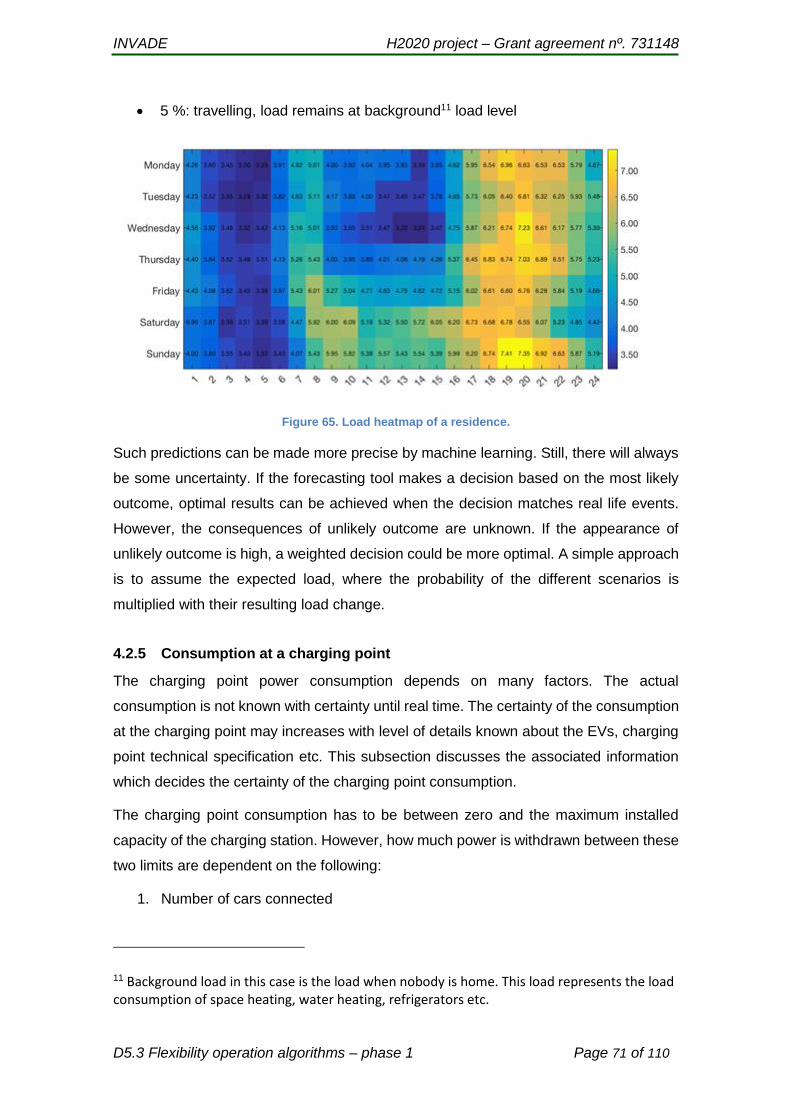
INVADE H2020 project – Grant agreement nº. 731148
D5.3 Flexibility operation algorithms – phase 1 Page 71 of 110
5 %: travelling, load remains at background11 load level
Figure 65. Load heatmap of a residence.
Such predictions can be made more precise by machine learning. Still, there will always
be some uncertainty. If the forecasting tool makes a decision based on the most likely
outcome, optimal results can be achieved when the decision matches real life events.
However, the consequences of unlikely outcome are unknown. If the appearance of
unlikely outcome is high, a weighted decision could be more optimal. A simple approach
is to assume the expected load, where the probability of the different scenarios is
multiplied with their resulting load change.
4.2.5 Consumption at a charging point
The charging point power consumption depends on many factors. The actual
consumption is not known with certainty until real time. The certainty of the consumption
at the charging point may increases with level of details known about the EVs, charging
point technical specification etc. This subsection discusses the associated information
which decides the certainty of the charging point consumption.
The charging point consumption has to be between zero and the maximum installed
capacity of the charging station. However, how much power is withdrawn between these
two limits are dependent on the following:
1. Number of cars connected
11 Background load in this case is the load when nobody is home. This load represents the load consumption of space heating, water heating, refrigerators etc.
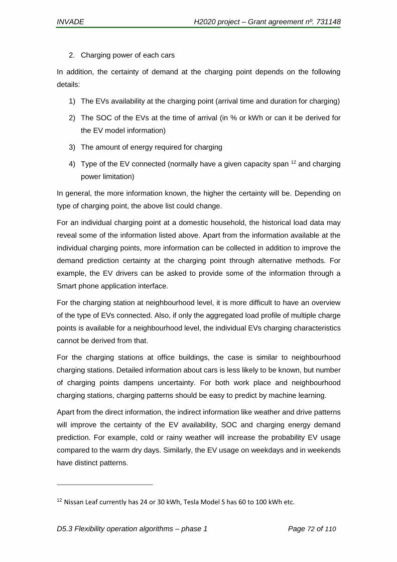
INVADE H2020 project – Grant agreement nº. 731148
D5.3 Flexibility operation algorithms – phase 1 Page 72 of 110
2. Charging power of each cars
In addition, the certainty of demand at the charging point depends on the following
details:
1) The EVs availability at the charging point (arrival time and duration for charging)
2) The SOC of the EVs at the time of arrival (in % or kWh or can it be derived for
the EV model information)
3) The amount of energy required for charging
4) Type of the EV connected (normally have a given capacity span 12 and charging
power limitation)
In general, the more information known, the higher the certainty will be. Depending on
type of charging point, the above list could change.
For an individual charging point at a domestic household, the historical load data may
reveal some of the information listed above. Apart from the information available at the
individual charging points, more information can be collected in addition to improve the
demand prediction certainty at the charging point through alternative methods. For
example, the EV drivers can be asked to provide some of the information through a
Smart phone application interface.
For the charging station at neighbourhood level, it is more difficult to have an overview
of the type of EVs connected. Also, if only the aggregated load profile of multiple charge
points is available for a neighbourhood level, the individual EVs charging characteristics
cannot be derived from that.
For the charging stations at office buildings, the case is similar to neighbourhood
charging stations. Detailed information about cars is less likely to be known, but number
of charging points dampens uncertainty. For both work place and neighbourhood
charging stations, charging patterns should be easy to predict by machine learning.
Apart from the direct information, the indirect information like weather and drive patterns
will improve the certainty of the EV availability, SOC and charging energy demand
prediction. For example, cold or rainy weather will increase the probability EV usage
compared to the warm dry days. Similarly, the EV usage on weekdays and in weekends
have distinct patterns.
12 Nissan Leaf currently has 24 or 30 kWh, Tesla Model S has 60 to 100 kWh etc.

INVADE H2020 project – Grant agreement nº. 731148
D5.3 Flexibility operation algorithms – phase 1 Page 73 of 110
For a public charging station, it is unlikely to have very specific information about each
EVs that connects (unless this is standardized). Again, the uncertainty on the aggregated
demand for charging decreases with the increased number of charging points inside a
given charging site. It is also likely that there is a correlation between charging and traffic
around the charging station, meaning that traffic forecasts could be utilized to predict
charging.
4.2.6 Prices
The electricity price will often be the most deciding decision factor to avail the flexibility
from the demand side and is therefore very important to know. The electricity price has
more than one component which influences the energy price. Some of the components
of the price changes more frequently and some changes lese frequently.
Grid tariffs:
Grid tariffs prices are fixed price the consumer pays as connecting charge to the grid for
their load capacity The grid tariff does not change every day or in hourly basis. Therefore,
the change in grid tariff affects the investment planning rather than the day today
operational optimization and planning.
Taxes:
Similar to the taxation on electricity usage changes very less frequently and therefore
affects the investment planning rather than the day today operational optimization and
planning
Spot price:
The electricity market spot price is the most uncertain type of price. Day-ahead prices
are normally published at noon, and contain hourly prices for the next day. This means
that if the optimization algorithm is run at 11.59 am, spot prices are only known for the
next 12 hours. However, if run 1 minute later at noon, day-ahead prices are published
and available for the entire next day, i.e 36 hours ahead. Small prosumer batteries can
normally do a full charging cycle in approximately 4 hours. In other words, decisions are
mostly decided by the price development in the next 4 hours of operation. Thus, the worst
case scenario where spot price is only known for the next 12 hours should not be a
problem. If it for some reason is required to know spot prices for more than the 12-36
hours that are available, some kind of spot price forecasting is required.
Figure 66. shows how the knowledge of future spot prices is depending on which hour
of the day we are in. The top example shows the scenario where we are running the
optimization at noon, just after day-ahead prices are released. The bottom example
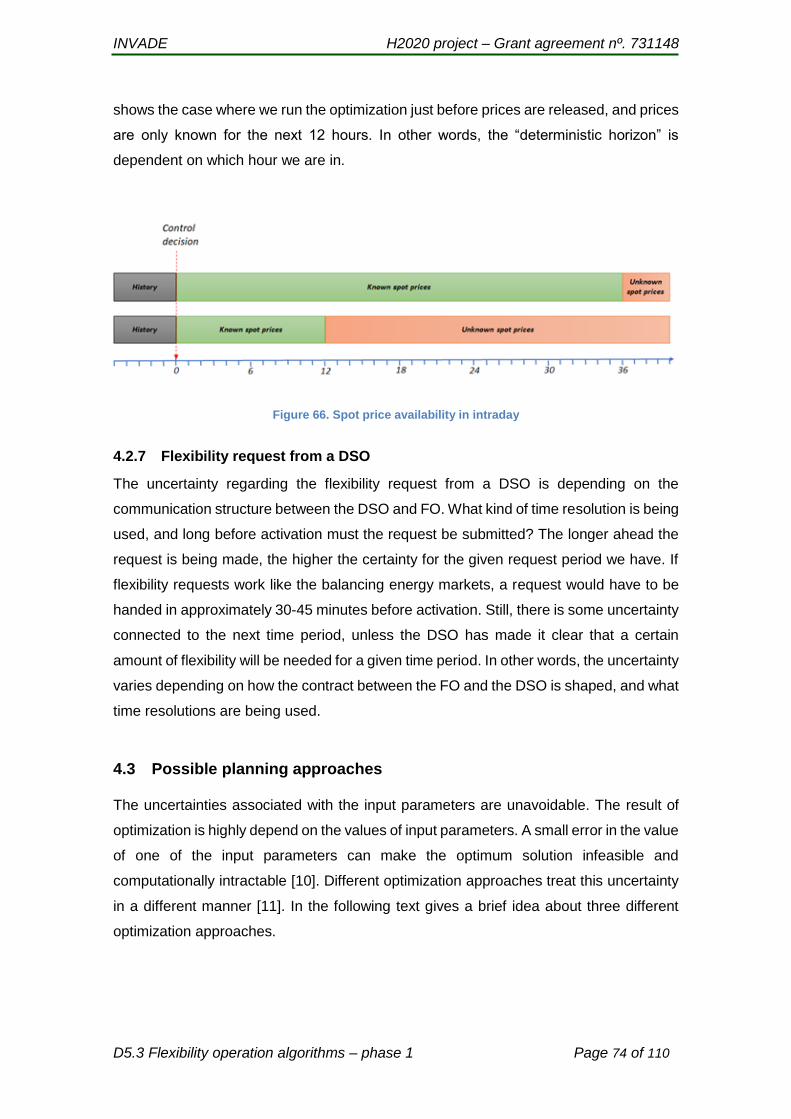
INVADE H2020 project – Grant agreement nº. 731148
D5.3 Flexibility operation algorithms – phase 1 Page 74 of 110
shows the case where we run the optimization just before prices are released, and prices
are only known for the next 12 hours. In other words, the “deterministic horizon” is
dependent on which hour we are in.
Figure 66. Spot price availability in intraday
4.2.7 Flexibility request from a DSO
The uncertainty regarding the flexibility request from a DSO is depending on the
communication structure between the DSO and FO. What kind of time resolution is being
used, and long before activation must the request be submitted? The longer ahead the
request is being made, the higher the certainty for the given request period we have. If
flexibility requests work like the balancing energy markets, a request would have to be
handed in approximately 30-45 minutes before activation. Still, there is some uncertainty
connected to the next time period, unless the DSO has made it clear that a certain
amount of flexibility will be needed for a given time period. In other words, the uncertainty
varies depending on how the contract between the FO and the DSO is shaped, and what
time resolutions are being used.
4.3 Possible planning approaches
The uncertainties associated with the input parameters are unavoidable. The result of
optimization is highly depend on the values of input parameters. A small error in the value
of one of the input parameters can make the optimum solution infeasible and
computationally intractable [10]. Different optimization approaches treat this uncertainty
in a different manner [11]. In the following text gives a brief idea about three different
optimization approaches.
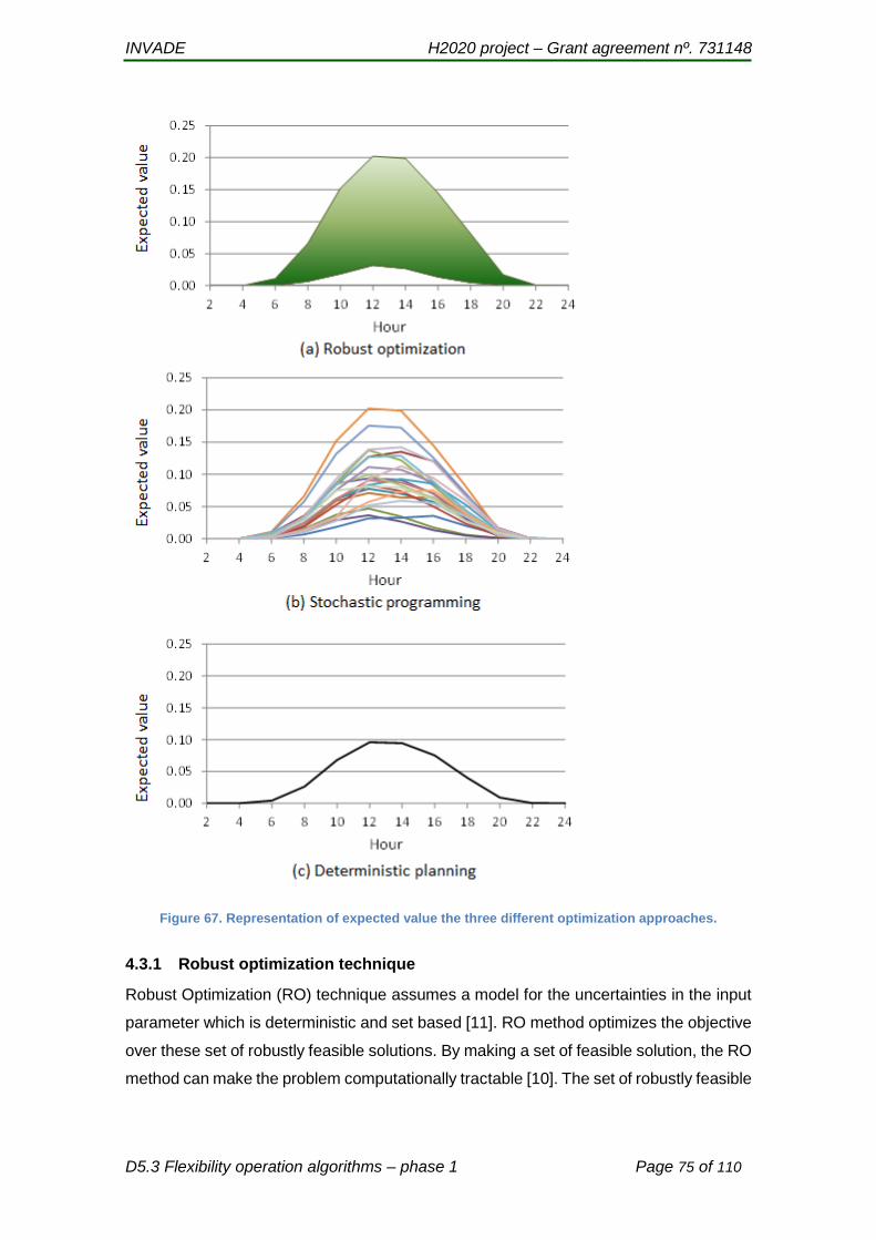
INVADE H2020 project – Grant agreement nº. 731148
D5.3 Flexibility operation algorithms – phase 1 Page 75 of 110
Figure 67. Representation of expected value the three different optimization approaches.
4.3.1 Robust optimization technique
Robust Optimization (RO) technique assumes a model for the uncertainties in the input
parameter which is deterministic and set based [11]. RO method optimizes the objective
over these set of robustly feasible solutions. By making a set of feasible solution, the RO
method can make the problem computationally tractable [10]. The set of robustly feasible

INVADE H2020 project – Grant agreement nº. 731148
D5.3 Flexibility operation algorithms – phase 1 Page 76 of 110
solutions guarantee to remain feasible for all uncertainty in the input parameters within
the set.
Thus, an optimal solution is available for all permissible values of input parameters within
the set. The solution obtained by RO method is not absolute optimal solution (global
optimum) for the given objective function [11]. This is the price paid for the robustness of
the solution for all possible inputs values. For example, the expected values of RO for a
PV plant to of certain installed capacity for the next 24 hours will be similar to Figure 67
(a). RO is best suited for the problems in which uncertainty matters, computational time
is valuable, estimation of probability distribution is difficult, and the decision should not
be risky.
4.3.2 Stochastic programming
In stochastic optimization, the assumption is that the uncertainties in the input
parameters have a probabilistic distribution. Within the probability distribution of the
uncertain input parameters, the objective function produces a collection of random
variables. The optimization process selects the best in these results, which satisfies the
objective function’s criterion. The stochastic optimization method tries to immunize the
solution in some probabilistic sense to this stochastic uncertainty. However, the
stochastic optimization always makes it feasible to achieve the solution, but the solution
obtained is only expected to be optimal for the given scenario. For example, the expected
values of stochastic programming for a PV plant of certain installed capacity for the next
24 hours will be similar to Figure 67 (b). The different expected value curves represents
different scenarios. The solution approach is based on the scenarios that are complex to
generate. This makes the stochastic optimization method to formulate the optimization
problem as a huge one with substantial data requirements [10].
4.3.3 Rolling horizon deterministic planning
The stochastic optimization assumes that there is random noise in the input parameters
and/or the choice is random to select the search direction when the algorithm starts to
iterate towards the solution (Monte Carlo) [11]. In contradictory, the deterministic method
assumes that a perfect information is available about the input parameters [11]. For
example, the expected values of deterministic programming for a PV plant to of certain
installed capacity for the next 24 hours will be similar to Figure 67 (c). With the available
information on the future values of the input parameters, the optimization process can

INVADE H2020 project – Grant agreement nº. 731148
D5.3 Flexibility operation algorithms – phase 1 Page 77 of 110
schedule the flexible and inflexible units (generation, load and storage) to certain time
horizon called planning horizon with multiple periods as shown in the Figure 68 (a).
Figure 68. Deterministic programming with rolling and receding methods.
The assumption is that the input parameters are more certain in these periods. Based
on the optimization decision, the control actions take place only for the immediate next
period or few nearest periods depends. In model predictive control (MPC) approaches,
it is always customary to make control decision for one time step and wait for the system
response to decide further control decisions (next time steps) [12], [13]. During the
present control execution period, the new update on some of the input parameters will
be available with more certainty than the previously available values. The new
optimization process will include the latest update on the input parameters and makes a
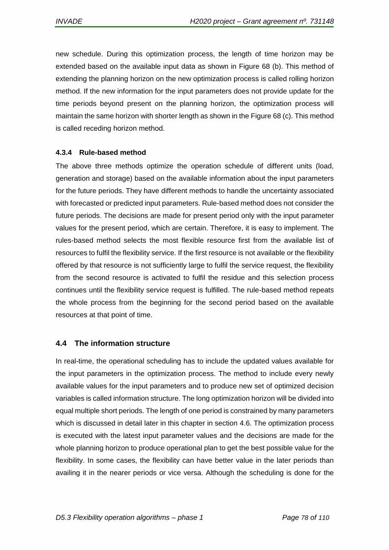
INVADE H2020 project – Grant agreement nº. 731148
D5.3 Flexibility operation algorithms – phase 1 Page 78 of 110
new schedule. During this optimization process, the length of time horizon may be
extended based on the available input data as shown in Figure 68 (b). This method of
extending the planning horizon on the new optimization process is called rolling horizon
method. If the new information for the input parameters does not provide update for the
time periods beyond present on the planning horizon, the optimization process will
maintain the same horizon with shorter length as shown in the Figure 68 (c). This method
is called receding horizon method.
4.3.4 Rule-based method
The above three methods optimize the operation schedule of different units (load,
generation and storage) based on the available information about the input parameters
for the future periods. They have different methods to handle the uncertainty associated
with forecasted or predicted input parameters. Rule-based method does not consider the
future periods. The decisions are made for present period only with the input parameter
values for the present period, which are certain. Therefore, it is easy to implement. The
rules-based method selects the most flexible resource first from the available list of
resources to fulfil the flexibility service. If the first resource is not available or the flexibility
offered by that resource is not sufficiently large to fulfil the service request, the flexibility
from the second resource is activated to fulfil the residue and this selection process
continues until the flexibility service request is fulfilled. The rule-based method repeats
the whole process from the beginning for the second period based on the available
resources at that point of time.
4.4 The information structure
In real-time, the operational scheduling has to include the updated values available for
the input parameters in the optimization process. The method to include every newly
available values for the input parameters and to produce new set of optimized decision
variables is called information structure. The long optimization horizon will be divided into
equal multiple short periods. The length of one period is constrained by many parameters
which is discussed in detail later in this chapter in section 4.6. The optimization process
is executed with the latest input parameter values and the decisions are made for the
whole planning horizon to produce operational plan to get the best possible value for the
flexibility. In some cases, the flexibility can have better value in the later periods than
availing it in the nearer periods or vice versa. Although the scheduling is done for the
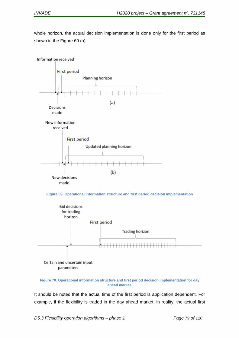
INVADE H2020 project – Grant agreement nº. 731148
D5.3 Flexibility operation algorithms – phase 1 Page 79 of 110
whole horizon, the actual decision implementation is done only for the first period as
shown in the Figure 69 (a).
Figure 69. Operational information structure and first period decision implementation
Figure 70. Operational information structure and first period decision implementation for day
ahead market.
It should be noted that the actual time of the first period is application dependent. For
example, if the flexibility is traded in the day ahead market, in reality, the actual first

INVADE H2020 project – Grant agreement nº. 731148
D5.3 Flexibility operation algorithms – phase 1 Page 80 of 110
period appears in the next day as shown in the Figure 70. The optimization process is
iterated whenever there is an update about the input parameter value and the new
schedule is produced and the process continues with first period decision implementation
structure as shown in the Figure 69 (b).
4.5 Length of the planning horizon
The optimization process is executed after every time a new information received and
the decisions are made for a number of periods in the planning horizon as shown in the
Figure 71. Many parameters have their influence on the length of planning horizon. It
depends on application, information availability and validity, error tolerance level of the
system, computation complexity of the optimization problem and length of the sub
periods within the planning horizon. Table 6 illustrates various applications with different
planning horizons and forecast methodologies.
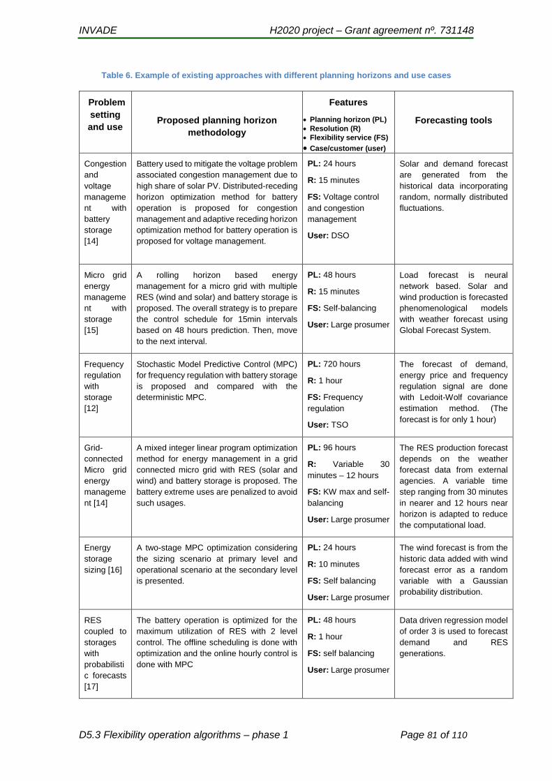
INVADE H2020 project – Grant agreement nº. 731148
D5.3 Flexibility operation algorithms – phase 1 Page 81 of 110
Table 6. Example of existing approaches with different planning horizons and use cases
Problem
setting
and use
Proposed planning horizon
methodology
Features
Planning horizon (PL)
Resolution (R)
Flexibility service (FS)
Case/customer (user)
Forecasting tools
Congestion
and
voltage
manageme
nt with
battery
storage
[14]
Battery used to mitigate the voltage problem
associated congestion management due to
high share of solar PV. Distributed-receding
horizon optimization method for battery
operation is proposed for congestion
management and adaptive receding horizon
optimization method for battery operation is
proposed for voltage management.
PL: 24 hours
R: 15 minutes
FS: Voltage control
and congestion
management
User: DSO
Solar and demand forecast
are generated from the
historical data incorporating
random, normally distributed
fluctuations.
Micro grid
energy
manageme
nt with
storage
[15]
A rolling horizon based energy
management for a micro grid with multiple
RES (wind and solar) and battery storage is
proposed. The overall strategy is to prepare
the control schedule for 15min intervals
based on 48 hours prediction. Then, move
to the next interval.
PL: 48 hours
R: 15 minutes
FS: Self-balancing
User: Large prosumer
Load forecast is neural
network based. Solar and
wind production is forecasted
phenomenological models
with weather forecast using
Global Forecast System.
Frequency
regulation
with
storage
[12]
Stochastic Model Predictive Control (MPC)
for frequency regulation with battery storage
is proposed and compared with the
deterministic MPC.
PL: 720 hours
R: 1 hour
FS: Frequency
regulation
User: TSO
The forecast of demand,
energy price and frequency
regulation signal are done
with Ledoit-Wolf covariance
estimation method. (The
forecast is for only 1 hour)
Grid-
connected
Micro grid
energy
manageme
nt [14]
A mixed integer linear program optimization
method for energy management in a grid
connected micro grid with RES (solar and
wind) and battery storage is proposed. The
battery extreme uses are penalized to avoid
such usages.
PL: 96 hours
R: Variable 30
minutes – 12 hours
FS: KW max and self-
balancing
User: Large prosumer
The RES production forecast
depends on the weather
forecast data from external
agencies. A variable time
step ranging from 30 minutes
in nearer and 12 hours near
horizon is adapted to reduce
the computational load.
Energy
storage
sizing [16]
A two-stage MPC optimization considering
the sizing scenario at primary level and
operational scenario at the secondary level
is presented.
PL: 24 hours
R: 10 minutes
FS: Self balancing
User: Large prosumer
The wind forecast is from the
historic data added with wind
forecast error as a random
variable with a Gaussian
probability distribution.
RES
coupled to
storages
with
probabilisti
c forecasts
[17]
The battery operation is optimized for the
maximum utilization of RES with 2 level
control. The offline scheduling is done with
optimization and the online hourly control is
done with MPC
PL: 48 hours
R: 1 hour
FS: self balancing
User: Large prosumer
Data driven regression model
of order 3 is used to forecast
demand and RES
generations.
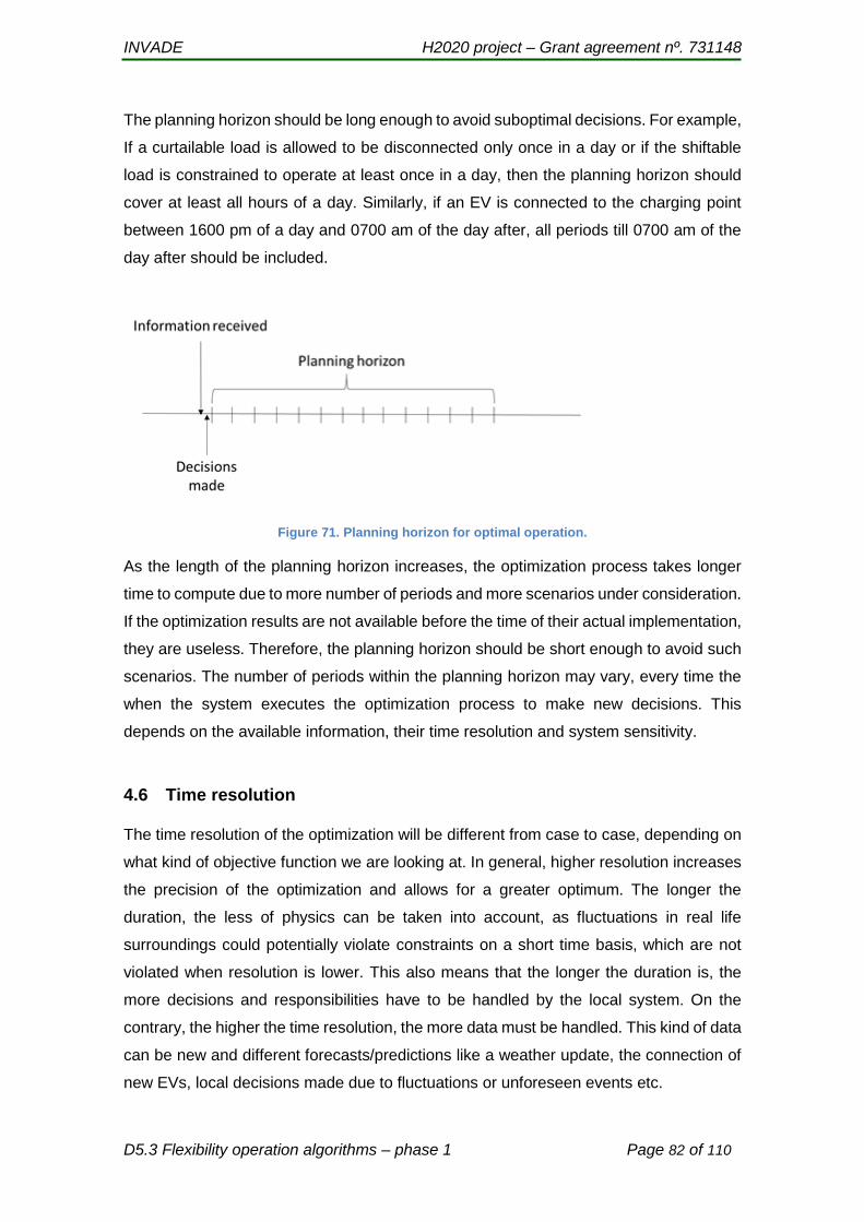
INVADE H2020 project – Grant agreement nº. 731148
D5.3 Flexibility operation algorithms – phase 1 Page 82 of 110
The planning horizon should be long enough to avoid suboptimal decisions. For example,
If a curtailable load is allowed to be disconnected only once in a day or if the shiftable
load is constrained to operate at least once in a day, then the planning horizon should
cover at least all hours of a day. Similarly, if an EV is connected to the charging point
between 1600 pm of a day and 0700 am of the day after, all periods till 0700 am of the
day after should be included.
Figure 71. Planning horizon for optimal operation.
As the length of the planning horizon increases, the optimization process takes longer
time to compute due to more number of periods and more scenarios under consideration.
If the optimization results are not available before the time of their actual implementation,
they are useless. Therefore, the planning horizon should be short enough to avoid such
scenarios. The number of periods within the planning horizon may vary, every time the
when the system executes the optimization process to make new decisions. This
depends on the available information, their time resolution and system sensitivity.
4.6 Time resolution
The time resolution of the optimization will be different from case to case, depending on
what kind of objective function we are looking at. In general, higher resolution increases
the precision of the optimization and allows for a greater optimum. The longer the
duration, the less of physics can be taken into account, as fluctuations in real life
surroundings could potentially violate constraints on a short time basis, which are not
violated when resolution is lower. This also means that the longer the duration is, the
more decisions and responsibilities have to be handled by the local system. On the
contrary, the higher the time resolution, the more data must be handled. This kind of data
can be new and different forecasts/predictions like a weather update, the connection of
new EVs, local decisions made due to fluctuations or unforeseen events etc.

INVADE H2020 project – Grant agreement nº. 731148
D5.3 Flexibility operation algorithms – phase 1 Page 83 of 110
Market rules play a role because they decide important factors such as spot price. For a
prosumer case, resolution can not be lower than the time resolution of the prize; 1 hour.
One could also change the time resolution depending on where in the time horizon it is.
For example, a 15 minute time resolution could be used for the next 6 hours, whereas 1
hour is used from 6 to 48 hours ahead as fine tuning is less relevant in the future where
uncertainty is greater. Such an approach would ensure optimal decisions in close time
horizon while still giving an indication of operation in a longer time perspective without
increasing the computational time too much.
4.6.1 Prosumer
In general, the time resolution should be equal to the factor that requires the highest
resolution. However, this is not always realizable. For example, an objective function
maximizing the profit (savings) of a prosumer, will need to take load, PV production and
price into account when deciding how to operate a battery, EV battery or other flexibility
services. Although the price is updated on an hourly basis, the PV and load can change
in a matter of seconds. What happens if an EV connects just after a new periods has
started? With a high time resolution, the EV can be integrated into the decisions quickly,
whereas a low time resolution the EV will not be taken into account before a new time
period starts. For some cases (e.g. home charging), this might not be a problem because
the car might be connected for a long time, whereas public charging stations would have
to provide some power to the EV right away. Still, it is not possible to make a new
optimization every minute. In other words, time resolution should be chosen to be a
reasonable value after analysing the benefits and drawbacks of different resolutions, and
if a time resolution is chosen which can’t handle specific real life events, some rule based
or simplified solution has to be made until a new period starts.
4.6.2 DSO
Congestion management services can only be provided within the same time resolution
of the model, meaning that if a 15 minute resolution is used, a request to provide flexibility
at 15:55 is not possible. For the DSO case, a time resolution of 15 minutes was used in
EMPOWER.
Congestion management and voltage control are problems mainly based on one factor:
consumer demand. In other words, the time resolution should be as high as the demand
changes, which due to the continuity of real life demand is impossible. The platform
needs to have a reasonable time resolution which can handle most of the problems

INVADE H2020 project – Grant agreement nº. 731148
D5.3 Flexibility operation algorithms – phase 1 Page 84 of 110
connected to congestion management and voltage fluctuations while still having a longer
time resolution than the computational time of the optimization.
4.6.3 BRP
For a BRP case, resolution would have to be minimum the resolution of the market. In
Norway, this is 1 hour, whereas it is 15 minutes in Germany. Minimum time resolution
would have to be changed accordingly.
4.7 Overall operational scheduling optimization process
Figure 72 shows the overview of the operational scheduling optimization process. The
optimization model receives input parameter values for consumption, generation and
available flexibility. These values are dynamic, depend of external factors and have
uncertainties associated with them. These values are derived from their historical data
and external information like electricity prices, weather forecast and booking information
of EV charge posts etc. The other fixed data structure, for example the installed
capacities of PV generation and battery storage, maximum charge/discharge powers
and network physical constraints are also fed to the optimization model. The result of
optimization is control decisions for the planning horizon. The results formatted to meet
the local generation, load and battery units’ communication protocol requirements and
communicated in a way to activate only the first period decisions. If the optimization
model complaints that the problem is infeasible, default control decisions will be followed.
Figure 72. Overview of the operational scheduling optimization process

INVADE H2020 project – Grant agreement nº. 731148
D5.3 Flexibility operation algorithms – phase 1 Page 85 of 110
5 Mathematical formulations
5.1 Overview of sets, parameters and variables
5.1.1 Sets
𝑇 Set of periods/time slots in the planning horizon
𝑇𝑐 Subset of periods where curtailment is allowed
𝐵 Set of battery units
𝑉 Set of electric vehicles
𝑉𝑖 Subset of electric vehicles that are inflexible
𝑉𝑠 Subset of electric vehicles that are shiftable
𝑉𝑑 Subset of electric vehicles that are disconnectable (shiftable interruptible)
𝑉𝑐 Subset of electric vehicles that are reducible (fully controllable)
𝑉2 Subset of electric vehicles that can be discharged (V2X)
𝐼 Set of load shift intervals
𝐿 Set of load units
𝐿𝑖 Subset of load units that are inflexible
𝐿𝑟 Subset of load units that are curtailable reducible
𝐿𝑑 Subset of load units that are curtailable disconnectable
𝐿𝑝 Subset of load units that are shiftable profile
𝐿𝑣 Subset of load units that are shiftable volume
𝐺 Set of generation units
𝐺𝑖 Subset of generation units that are inflexible
𝐺𝑟 Subset of generation units that are curtailable reducible
𝐺𝑑 Subset of generation units that are curtailable disconnectable

INVADE H2020 project – Grant agreement nº. 731148
D5.3 Flexibility operation algorithms – phase 1 Page 86 of 110
5.1.2 Parameters
𝑃𝑡𝑟𝑒𝑡𝑎𝑖𝑙−𝑏𝑢𝑦
Price at energy part of retail contract for buying electricity in period t
[€/kWh]
𝑃𝑡𝑔𝑟𝑖𝑑−𝑏𝑢𝑦
Price at energy part of grid contract for buying electricity in period t
[€/kWh]
𝑃𝑡𝑔𝑟𝑖𝑑−𝑏𝑢𝑦−𝑙𝑜𝑤
Price at energy part of grid contract for buying electricity in cases with
subscribed power in period in period t if bought electricity is below
subscribed level [€/kWh]
𝑃𝑡𝑔𝑟𝑖𝑑−𝑏𝑢𝑦−ℎ𝑖𝑔ℎ
Price at energy part of grid contract for buying electricity in cases with
subscribed power in period in period t if bought electricity is above
subscribed level [€/kWh]
𝑃𝑡𝑎𝑥 Sum price for all taxes that are related to buying electricity in period t
[€/kWh]
𝑃𝑉𝐴𝑇 Parameter that adds VAT to the amount bought [fraction]
𝑃𝑡𝑟𝑒𝑡𝑎𝑖𝑙−𝑠𝑒𝑙𝑙 Price at energy part of retail contract for selling electricity in period t
[€/kWh]
𝑃𝑡𝑔𝑟𝑖𝑑−𝑠𝑒𝑙𝑙
Price at energy part of grid contract for selling electricity in period t
[€/kWh]
𝑃𝑝𝑒𝑎𝑘 Price at grid contract for peak fee [€/kW/month]
𝑋𝑖𝑚𝑝−𝑐𝑎𝑝 Maximum import capacity [average kW]
𝑋𝑒𝑥𝑝−𝑐𝑎𝑝 Maximum export capacity [average kW]
𝑀 Limitation of basis for peak fee [kW]
𝑂𝑏𝑚𝑖𝑛 Minimum state of charge allowed for battery b [kWh]
𝑂𝑏𝑚𝑎𝑥 Maximum state of charge allowed for battery b [kWh]
𝑂𝑣𝐸𝑉,𝑚𝑖𝑛 Minimum state of charge allowed for EV unit v [kWh]
𝑂𝑣𝐸𝑉,𝑚𝑎𝑥 Maximum state of charge allowed for EV unit v [kWh]
𝑂𝑣,𝑡𝐸𝑉,𝑚𝑖𝑛,𝑡 Minimum state of charge allowed for EV unit v at period t [kWh]
𝑂𝑣𝐶𝐷 Total charging demand for EV unit v [kWh]
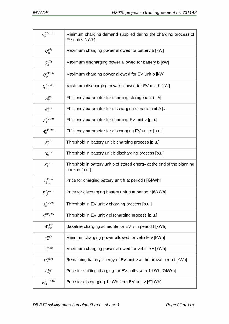
INVADE H2020 project – Grant agreement nº. 731148
D5.3 Flexibility operation algorithms – phase 1 Page 87 of 110
𝑂𝑣𝐶𝐷,𝑚𝑖𝑛
Minimum charging demand supplied during the charging process of
EV unit v [kWh]
𝑄𝑏𝑐ℎ Maximum charging power allowed for battery b [kW]
𝑄𝑏𝑑𝑖𝑠 Maximum discharging power allowed for battery b [kW]
𝑄𝑣𝐸𝑉,𝑐ℎ Maximum charging power allowed for EV unit b [kW]
𝑄𝑣𝐸𝑉,𝑑𝑖𝑠 Maximum discharging power allowed for EV unit b [kW]
𝐴𝑏𝑐ℎ Efficiency parameter for charging storage unit b [#]
𝐴𝑏𝑑𝑖𝑠 Efficiency parameter for discharging storage unit b [#]
𝐴𝑣𝐸𝑉,𝑐ℎ Efficiency parameter for charging EV unit v [p.u.]
𝐴𝑣𝐸𝑉,𝑑𝑖𝑠 Efficiency parameter for discharging EV unit v [p.u.]
𝑆𝑏𝑐ℎ Threshold in battery unit b charging process [p.u.]
𝑆𝑏𝑑𝑖𝑠 Threshold in battery unit b discharging process [p.u.]
𝑆𝑏𝑒𝑛𝑑 Threshold in battery unit b of stored energy at the end of the planning
horizon [p.u.]
𝑃𝑏,𝑡𝐵,𝑐ℎ
Price for charging battery unit b at period t [€/kWh]
𝑃𝑏,𝑡𝐵,𝑑𝑖𝑠𝑐 Price for discharging battery unit b at period t [€/kWh]
𝑆𝑣𝐸𝑉,𝑐ℎ Threshold in EV unit v charging process [p.u.]
𝑆𝑣𝐸𝑉,𝑑𝑖𝑠 Threshold in EV unit v discharging process [p.u.]
𝑊𝑣,𝑡𝐸𝑉 Baseline charging schedule for EV v in period t [kWh]
𝐸𝑣𝑚𝑖𝑛 Minimum charging power allowed for vehicle v [kWh]
𝐸𝑣𝑚𝑎𝑥 Maximum charging power allowed for vehicle v [kWh]
𝐸𝑣𝑠𝑡𝑎𝑟𝑡 Remaining battery energy of EV unit v at the arrival period [kWh]
𝑃𝑣,𝑡𝐸𝑉 Price for shifting charging for EV unit v with 1 kWh [€/kWh]
𝑃𝑣,𝑡𝐸𝑉,𝑉2𝐺 Price for discharging 1 kWh from EV unit v [€/kWh]
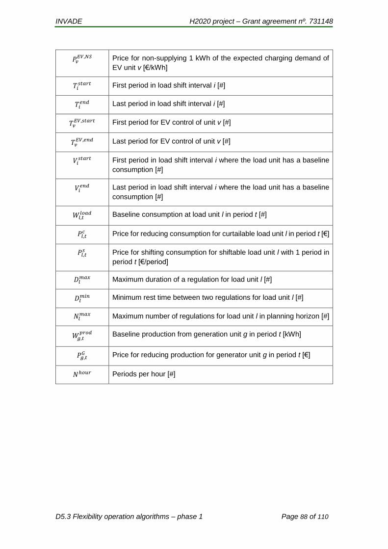
INVADE H2020 project – Grant agreement nº. 731148
D5.3 Flexibility operation algorithms – phase 1 Page 88 of 110
𝑃𝑣𝐸𝑉,𝑁𝑆
Price for non-supplying 1 kWh of the expected charging demand of
EV unit v [€/kWh]
𝑇𝑖𝑠𝑡𝑎𝑟𝑡 First period in load shift interval i [#]
𝑇𝑖𝑒𝑛𝑑 Last period in load shift interval i [#]
𝑇𝑣𝐸𝑉,𝑠𝑡𝑎𝑟𝑡 First period for EV control of unit v [#]
𝑇𝑣𝐸𝑉,𝑒𝑛𝑑 Last period for EV control of unit v [#]
𝑉𝑖𝑠𝑡𝑎𝑟𝑡 First period in load shift interval i where the load unit has a baseline
consumption [#]
𝑉𝑖𝑒𝑛𝑑 Last period in load shift interval i where the load unit has a baseline
consumption [#]
𝑊𝑙,𝑡𝑙𝑜𝑎𝑑 Baseline consumption at load unit l in period t [#]
𝑃𝑙,𝑡𝑐 Price for reducing consumption for curtailable load unit l in period t [€]
𝑃𝑙,𝑡𝑠 Price for shifting consumption for shiftable load unit l with 1 period in
period t [€/period]
𝐷𝑙𝑚𝑎𝑥 Maximum duration of a regulation for load unit l [#]
𝐷𝑙𝑚𝑖𝑛 Minimum rest time between two regulations for load unit l [#]
𝑁𝑙𝑚𝑎𝑥 Maximum number of regulations for load unit l in planning horizon [#]
𝑊𝑔,𝑡𝑝𝑟𝑜𝑑
Baseline production from generation unit g in period t [kWh]
𝑃𝑔,𝑡𝐺 Price for reducing production for generator unit g in period t [€]
𝑁ℎ𝑜𝑢𝑟 Periods per hour [#]
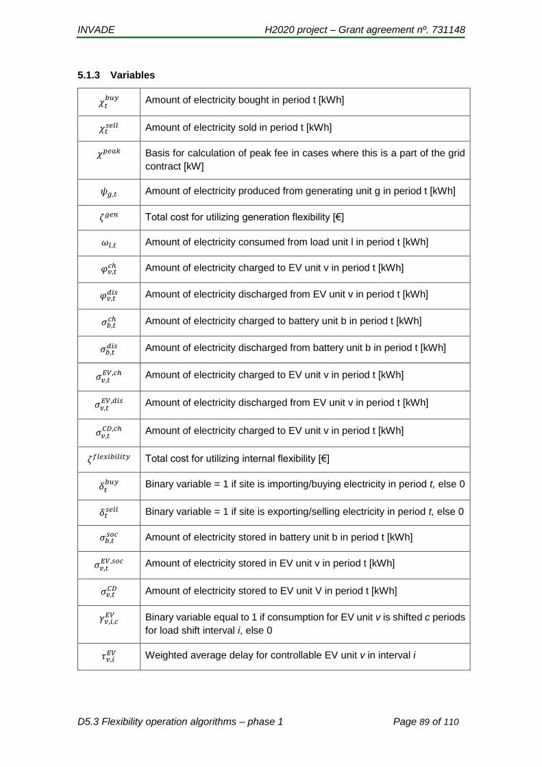
INVADE H2020 project – Grant agreement nº. 731148
D5.3 Flexibility operation algorithms – phase 1 Page 89 of 110
5.1.3 Variables
𝜒𝑡𝑏𝑢𝑦
Amount of electricity bought in period t [kWh]
𝜒𝑡𝑠𝑒𝑙𝑙 Amount of electricity sold in period t [kWh]
𝜒𝑝𝑒𝑎𝑘 Basis for calculation of peak fee in cases where this is a part of the grid
contract [kW]
𝜓𝑔,𝑡 Amount of electricity produced from generating unit g in period t [kWh]
𝜁𝑔𝑒𝑛 Total cost for utilizing generation flexibility [€]
𝜔𝑙,𝑡 Amount of electricity consumed from load unit l in period t [kWh]
𝜑𝑣,𝑡𝑐ℎ Amount of electricity charged to EV unit v in period t [kWh]
𝜑𝑣,𝑡𝑑𝑖𝑠 Amount of electricity discharged from EV unit v in period t [kWh]
𝜎𝑏,𝑡𝑐ℎ Amount of electricity charged to battery unit b in period t [kWh]
𝜎𝑏,𝑡𝑑𝑖𝑠 Amount of electricity discharged from battery unit b in period t [kWh]
𝜎𝑣,𝑡𝐸𝑉,𝑐ℎ Amount of electricity charged to EV unit v in period t [kWh]
𝜎𝑣,𝑡𝐸𝑉,𝑑𝑖𝑠 Amount of electricity discharged from EV unit v in period t [kWh]
𝜎𝑣,𝑡𝐶𝐷,𝑐ℎ Amount of electricity charged to EV unit v in period t [kWh]
𝜁𝑓𝑙𝑒𝑥𝑖𝑏𝑖𝑙𝑖𝑡𝑦 Total cost for utilizing internal flexibility [€]
𝛿𝑡𝑏𝑢𝑦
Binary variable = 1 if site is importing/buying electricity in period t, else 0
𝛿𝑡𝑠𝑒𝑙𝑙 Binary variable = 1 if site is exporting/selling electricity in period t, else 0
𝜎𝑏,𝑡𝑠𝑜𝑐 Amount of electricity stored in battery unit b in period t [kWh]
𝜎𝑣,𝑡𝐸𝑉,𝑠𝑜𝑐 Amount of electricity stored in EV unit v in period t [kWh]
𝜎𝑣,𝑡𝐶𝐷 Amount of electricity stored to EV unit V in period t [kWh]
𝛾𝑣,𝑖,𝑐𝐸𝑉 Binary variable equal to 1 if consumption for EV unit v is shifted c periods
for load shift interval i, else 0
𝜏𝑣,𝑖𝐸𝑉 Weighted average delay for controllable EV unit v in interval i

INVADE H2020 project – Grant agreement nº. 731148
D5.3 Flexibility operation algorithms – phase 1 Page 90 of 110
𝜌𝑣,𝑖𝐸𝑉 Help variable to handle positive and negative values of 𝜏𝑣,𝑖
𝐸𝑉
𝜁𝐸𝑉,𝑠ℎ𝑖𝑓𝑡 Cost for shifting EV charging [€]
𝜁𝐸𝑉,𝑐𝑜𝑛𝑡𝑟𝑜𝑙 Cost for controlling EV charging [€]
𝜁𝐸𝑉,𝑉2𝑋 Cost for controlling EV charging and discharging [€]
𝛿𝑙,𝑡𝑠𝑡𝑎𝑟𝑡 Binary variable equal to 1 if regulation of load unit l starts in the beginning
of period t, else 0
𝛿𝑙,𝑡𝑟𝑢𝑛 Binary variable equal to 1 if regulation of load unit l is running in period t,
else 0
𝛿𝑙,𝑡𝑒𝑛𝑑 Binary variable equal to 1 if regulation of load unit l ends in the beginning
of period t, else 0
𝛾𝑙,𝑖,𝑐𝑙𝑜𝑎𝑑 Binary variable equal to 1 if consumption for load unit l is shifted c periods
for load shift interval i, else 0
𝜏𝑙,𝑖𝑙𝑜𝑎𝑑 Weighted average delay for shiftable load unit l in interval i
𝜌𝑙,𝑖𝑙𝑜𝑎𝑑 Help variable to handle positive and negative values of 𝜏𝑙,𝑖
𝑙𝑜𝑎𝑑
𝜁𝑙𝑜𝑎𝑑𝑐𝑢𝑟𝑡𝑎𝑖𝑙 Cost for curtailing load [€]
𝜁𝑙𝑜𝑎𝑑𝑠ℎ𝑖𝑓𝑡 Cost for shifting load [€]
𝛿𝑔,𝑡𝑔𝑒𝑛
Binary variable equal to 0 if generating unit g is disconnected in period t,
else 1
5.2 Common/general constraints
5.2.1 Battery models
Each battery unit b has efficiency factors for charging 𝐴𝑏𝑐ℎ and discharging 𝐴𝑏
𝑑𝑖𝑠,
respectively. The battery state of charge, i.e. the storage content, 𝜎𝑏,𝑡𝑠𝑜𝑐 for battery unit b
in period t depends on the state of charge in the previous period, and charging 𝜎𝑏,𝑡𝑐ℎ or
discharging 𝜎𝑏,𝑡𝑑𝑖𝑠 in current period.
𝜎𝑏,𝑡𝑠𝑜𝑐 = 𝜎𝑏,𝑡−1
𝑠𝑜𝑐 + 𝜎𝑏,𝑡𝑐ℎ ∗ 𝐴𝑏
𝑐ℎ −𝜎𝑏,𝑡
𝑑𝑖𝑠
𝐴𝑏𝑑𝑖𝑠
, ∀ 𝑏 ∈ 𝐵, 𝑡 ∈ 𝑇 (Eq. 1)

INVADE H2020 project – Grant agreement nº. 731148
D5.3 Flexibility operation algorithms – phase 1 Page 91 of 110
The state of charge must be within minimum and maximum limits:
Charging and discharging must be below maximum charging levels:
Previous constraints assume that the batteries are completely adjustable in terms of
power input and output up to the maximum power specified 𝑄𝑏𝑐ℎ and 𝑄𝑏
𝑑𝑖𝑠.
However, the following constraint ensures that the energy charged 𝜎𝑏,𝑡𝑐ℎ to the battery b
is linearly decreased from 𝑆𝑏𝑐ℎ state-of-charge, typically 0.8 (80%), until zero at 100%
SOC.
Figure 73. Battery state of charge as a function of maximum charging power
The same for discharging power 𝜎𝑏,𝑡,𝑠𝑜𝑢𝑡 of battery unit b during period t. The lower
threshold to limit the energy output is 𝑆𝑏𝑑𝑖𝑠, typically 0.1 (10% SOC), until zero power
output at 0% SOC.
0
2
4
6
8
10
12
0.0% 20.0% 40.0% 60.0% 80.0% 100.0%
Max
imu
m c
har
gin
g p
ow
er
Battery state of charge
O^in
constraint 16Mouli2017
Maximum chargingpower
𝑂𝑏𝑚𝑖𝑛 ≤ 𝜎𝑏,𝑡
𝑠𝑜𝑐≤ 𝑂𝑏
𝑚𝑎𝑥, ∀ 𝑏 ∈ 𝐵, 𝑡 ∈ 𝑇 (Eq. 2)
𝜎𝑏,𝑡𝑐ℎ ≤
𝑄𝑏𝑐ℎ
𝑁ℎ𝑜𝑢𝑟, ∀ 𝑏 ∈ 𝐵, 𝑡 ∈ 𝑇 (Eq. 3)
𝜎𝑏,𝑡𝑑𝑖𝑠 ≤
𝑄𝑏𝑑𝑖𝑠
𝑁ℎ𝑜𝑢𝑟, ∀ 𝑏 ∈ 𝐵, 𝑡 ∈ 𝑇 (Eq. 4)
𝜎𝑏,𝑡𝑐ℎ ≤
−𝑄𝑏𝑐ℎ
𝑁ℎ𝑜𝑢𝑟⁄
1 − 𝑆𝑏𝑐ℎ (
𝜎𝑏,𝑡𝑠𝑜𝑐
𝑂𝑏𝑚𝑎𝑥 − 1)
(Eq. 5)
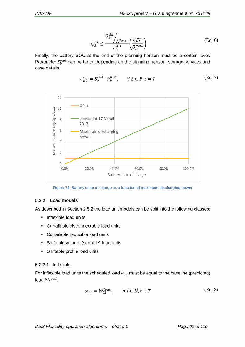
INVADE H2020 project – Grant agreement nº. 731148
D5.3 Flexibility operation algorithms – phase 1 Page 92 of 110
Finally, the battery SOC at the end of the planning horizon must be a certain level.
Parameter 𝑆𝑏𝑒𝑛𝑑 can be tuned depending on the planning horizon, storage services and
case details.
Figure 74. Battery state of charge as a function of maximum discharging power
5.2.2 Load models
As described in Section 2.5.2 the load unit models can be split into the following classes:
Inflexible load units
Curtailable disconnectable load units
Curtailable reducible load units
Shiftable volume (storable) load units
Shiftable profile load units
5.2.2.1 Inflexible
For inflexible load units the scheduled load 𝜔𝑙,𝑡 must be equal to the baseline (predicted)
load 𝑊𝑙,𝑡𝑙𝑜𝑎𝑑.
0
2
4
6
8
10
12
0.0% 20.0% 40.0% 60.0% 80.0% 100.0%
Max
imu
m d
isch
argi
ng
po
wer
Battery state of charge
O^in
constraint 17 Mouli2017
Maximum dischargingpower
𝜎𝑏,𝑡𝑜𝑢𝑡 ≤
𝑄𝑏𝑑𝑖𝑠
𝑁ℎ𝑜𝑢𝑟⁄
𝑆𝑏𝑑𝑖𝑠
(𝜎𝑏,𝑡
𝑠𝑜𝑐
𝑂𝑏𝑚𝑎𝑥)
(Eq. 6)
𝜎𝑏,𝑡𝑠𝑜𝑐 = 𝑆𝑏
𝑒𝑛𝑑 · 𝑂𝑏𝑚𝑎𝑥, ∀ 𝑏 ∈ 𝐵, 𝑡 = 𝑇 (Eq. 7)
𝜔𝑙,𝑡 = 𝑊𝑙,𝑡𝑙𝑜𝑎𝑑, ∀ 𝑙 ∈ 𝐿𝑖 , 𝑡 ∈ 𝑇 (Eq. 8)

INVADE H2020 project – Grant agreement nº. 731148
D5.3 Flexibility operation algorithms – phase 1 Page 93 of 110
5.2.2.2 Curtailable
We introduce binary variables 𝛿𝑙,𝑡𝑠𝑡𝑎𝑟𝑡equal to 1 if load unit l starts regulation in the
beginning of period t, 𝛿𝑙,𝑡𝑟𝑢𝑛 equal to 1 in periods where regulation runs after the starting
period and finally, 𝛿𝑙,𝑡𝑒𝑛𝑑 equal to 1 in the first period after a regulation is stopped.
A curtailment can start or run only in permitted periods:
A curtailment can not start, run and end in the same period:
A curtailment that starts or runs in one period, must either continue to run or end in the
consecutive period:
A load unit can not be curtailed any longer than 𝐷𝑙𝑚𝑎𝑥periods:
A minimum duration 𝐷𝑙𝑚𝑖𝑛 must exist between two load curtailments:
The maximum number of curtailments in the planning horizon must not be greater than
𝑁𝑙,𝑖𝑚𝑎𝑥:
We illustrate the constraints with a small example. A load unit is curtailed in periods 1 to
4 and 7 to 8. The values of the binary variables are then as shown in the table below.
𝛿𝑙,𝑡𝑠𝑡𝑎𝑟𝑡 + 𝛿𝑙,𝑡
𝑟𝑢𝑛 = 0 ∀ 𝑙 ∈ 𝐿𝑐 , 𝑡 ∉ 𝑇𝑐 (Eq. 9)
𝛿𝑙,𝑡𝑠𝑡𝑎𝑟𝑡 + 𝛿𝑙,𝑡
𝑟𝑢𝑛 + 𝛿𝑙,𝑡𝑒𝑛𝑑 ≤ 1 ∀ 𝑙 ∈ 𝐿𝑐 , 𝑡 ∈ 𝑇 (Eq. 10)
𝛿𝑙,𝑡−1𝑠𝑡𝑎𝑟𝑡 + 𝛿𝑙,𝑡−1
𝑟𝑢𝑛 = 𝛿𝑙,𝑡𝑟𝑢𝑛 + 𝛿𝑙,𝑡
𝑒𝑛𝑑 ∀ 𝑙 ∈ 𝐿𝑐 , 𝑡 ∈ 𝑇 (Eq. 11)
∑ 𝛿𝑙,𝑖𝑒𝑛𝑑
𝑡+𝐷𝑙𝑚𝑎𝑥
𝑖=𝑡
≥ 𝛿𝑙,𝑖𝑠𝑡𝑎𝑟𝑡 ∀ 𝑙 ∈ 𝐿𝑐 , 𝑡 ∈ 𝑇
(Eq. 12)
𝛿𝑙,𝑡𝑒𝑛𝑑 + ∑ 𝛿𝑙,𝑖
𝑠𝑡𝑎𝑟𝑡
𝑡+𝐷𝑙𝑚𝑖𝑛−1
𝑖=𝑡
≤ 1 ∀ 𝑙 ∈ 𝐿𝑐 , 𝑡 ∈ 𝑇 (Eq. 13)
∑ 𝛿𝑙,𝑡𝑠𝑡𝑎𝑟𝑡
𝑡∈𝑇
≤ 𝑁𝑙𝑚𝑎𝑥 ∀ 𝑙 ∈ 𝐿𝑐, 𝑡 ∈ 𝑇 (Eq. 14)

INVADE H2020 project – Grant agreement nº. 731148
D5.3 Flexibility operation algorithms – phase 1 Page 94 of 110
Table 7. Example of binary variables for curtailable load units
1 2 3 4 5 6 7 8 9
𝛿𝑙,𝑡𝑠𝑡𝑎𝑟𝑡 1 0 0 0 0 0 1 0 0
𝛿𝑙,𝑡𝑟𝑢𝑛 0 1 1 1 0 0 0 1 0
𝛿𝑙,𝑡𝑒𝑛𝑑 0 0 0 0 1 0 0 0 1
The first curtailment starts in period 1, hence 𝛿𝑙,1𝑠𝑡𝑎𝑟𝑡 is set to 1. The curtailment continues
in periods 2, 3 and 4, and the 𝛿𝑙,𝑡𝑟𝑢𝑛 are set to 1. The curtailment stops in the beginning
of period 5 (or actually, in the end of period 4) so 𝛿𝑙,5𝑒𝑛𝑑 = 1.
For reducible load units, the load schedule 𝜒𝑙,𝑡 must be smaller than the consumption
forecast 𝑊𝑙,𝑡𝑙𝑜𝑎𝑑:
For disconnectable load units, the load schedule must either be 0 or equal to the
consumption forecast:
Curtailable load units will have a cost equal to the curtailment price multiplied with the
number of periods curtailed:
5.2.2.3 Shiftable
For shiftable load units we introduce load shift intervals l similar to the charging sessions
for the EVs.
For shiftable profile load units we introduce the variable 𝛾𝑙,𝑖,𝑛 which is set to 1 if
consumption for load unit l is shifted n periods for load shift interval i. Exactly one load
shifting option must selected for each shiftable profile load unit in each load shift interval:
𝜒𝑙,𝑡 ≤ (𝛿𝑙,𝑡𝑠𝑡𝑎𝑟𝑡 + 𝛿𝑙,𝑡
𝑟𝑢𝑛) ∗ 𝑊𝑙,𝑡𝑙𝑜𝑎𝑑, ∀ 𝑙 ∈ 𝐿𝑐 , 𝑡 ∈ 𝑇
(Eq. 15)
𝜒𝑙,𝑡 = (𝛿𝑙,𝑡𝑠𝑡𝑎𝑟𝑡 + 𝛿𝑙,𝑡
𝑟𝑢𝑛) ∗ 𝑊𝑙,𝑡𝑙𝑜𝑎𝑑, ∀ 𝑙 ∈ 𝐿𝑐 , 𝑡 ∈ 𝑇 (Eq. 16)
𝜁𝑙𝑜𝑎𝑑𝑐𝑢𝑟𝑡𝑎𝑖𝑙 = ∑ ∑ 𝑃𝑙,𝑡𝑙𝑜𝑎𝑑
𝑙∈𝑙𝑐
(𝛿𝑙,𝑡𝑠𝑡𝑎𝑟𝑡 + 𝛿𝑙,𝑡
𝑟𝑢𝑛)
𝑡∈𝑇
(Eq. 17)

INVADE H2020 project – Grant agreement nº. 731148
D5.3 Flexibility operation algorithms – phase 1 Page 95 of 110
The consumption forecasts must be allocated to the correct periods according to the
decided load shifting option:
For shiftable profile load units, the cost for regulation is the product of the delay cost and
the number of periods delayed. We calculate this cost according to the equation below:
Contrary to shiftable profile load units, for shiftable volume load units we can control the
power levels between a minimum 𝐸𝑙𝑚𝑖𝑛 and a maximum 𝐸𝑙
𝑚𝑎𝑥 value.
In some cases, similar to charging of EVs, 𝜔𝑙,𝑡 may be semi-continuous, which means
that it must be according to Eq. 36 or 0.
For each load shift interval i the sum energy volume delivered to the load unit must equal
the sum baseline forecast.
For shiftable volume load units, we introduce the concept of weighted average delay,
which has number of periods as unit. This also takes into account not only when you
meet the finale volume, but also how you do it (penalizes more if large volumes are
shifted to the end). The weighted average delay for shiftable load unit l and load shift
interval i is defined like as:
∑ 𝛾𝑙,𝑖,𝑛
𝑇𝑖𝑒𝑛𝑑−𝑉𝑖
𝑒𝑛𝑑
𝑛=𝑇𝑖𝑠𝑡𝑎𝑟𝑡−𝑉𝑖
𝑠𝑡𝑎𝑟𝑡
= 1 ∀ 𝑙 ∈ 𝐿𝑝, 𝑖 ∈ 𝐼(𝑙) (Eq. 18)
𝜔𝑙,𝑡= ∑ 𝛾𝑙,𝑖,(𝑡−𝑇𝑙,𝑖𝑠𝑡𝑎𝑟𝑡−𝑛)𝑊𝑙,(𝑇𝑙,𝑖
𝑠𝑡𝑎𝑟𝑡+𝑛)
𝑇𝑖𝑒𝑛𝑑−𝑇𝑖
𝑠𝑡𝑎𝑟𝑡
𝑛=0
∀ 𝑡 ∈ {𝑇𝑖𝑠𝑡𝑎𝑟𝑡, 𝑇𝑖
𝑒𝑛𝑑}, 𝑖 ∈ 𝐼(𝑙) (Eq. 19)
𝜁𝑙𝑜𝑎𝑑𝑝𝑟𝑜𝑓𝑖𝑙𝑒 = ∑ ∑ 𝑃𝑑𝑠 ∑ 𝛾𝑙,𝑖,𝑛
𝑙𝑜𝑎𝑑
𝑇𝑖𝑒𝑛𝑑−𝑉𝑖
𝑒𝑛𝑑
𝑛=0
𝑛
𝑖∈𝐼𝑙∈𝐿𝑝
(Eq. 20)
𝐸𝑙𝑚𝑖𝑛 ≤ 𝜔𝑙,𝑡 ≤ 𝐸𝑙
𝑚𝑎𝑥, ∀ 𝑙 ∈ 𝐿𝑣 , 𝑡 ∈ 𝑇(𝑖) (Eq. 21)
∑ 𝜔𝑙,𝑡
𝑇𝑖𝑒𝑛𝑑
𝑡=𝑇𝑖𝑠𝑡𝑎𝑟𝑡
= ∑ 𝑊𝑙,𝑡𝑙𝑜𝑎𝑑
𝑇𝑖𝑒𝑛𝑑
𝑡=𝑇𝑖𝑠𝑡𝑎𝑟𝑡
∀ 𝑙 ∈ 𝐿𝑣 , 𝑡 ∈ 𝑇(𝑖), 𝑖 ∈ 𝐼(𝑙) (Eq. 22)

INVADE H2020 project – Grant agreement nº. 731148
D5.3 Flexibility operation algorithms – phase 1 Page 96 of 110
Since this weighted average delay also may be negative (by shifting volume backwards),
we introduce a new variable 𝜌𝑙,𝑖𝑙𝑜𝑎𝑑 defined as:
The total costs for shifting volume load is then:
5.2.3 EV models
The present EV model has been developed with the purpose of finding the optimal
dispatch for charging the EV in a private charging station to provide flexibility services to
prosumer, DOS or BRP.
the constraints given both by the EV owner or external agents like DSO or BRP at private
stations, typically at home. Public installations could require a different approach.
Similar to generation units and load units the EV charging process may also have
different degrees and types of flexibility:
Inflexible EVs
Shiftable
Controllable
Controllable and interruptible
V2X
5.2.3.1 Inflexible EVs
For inflexible EVs (𝑣 ∈ 𝑉𝑖), i.e. EVs where the charging process cannot be controlled,
the charging 𝜑𝑣,𝑡𝑐ℎ scheduled to be delivered to EV v in period t is equal to the predicted
charging demand 𝑊𝑣,𝑡𝐸𝑉.
5.2.3.2 Shiftable
For shiftable EV units 𝑣 ∈ 𝑉𝑠 we introduce the term charging session 𝑖 ∈ 𝐼(𝑣), defined by
connection 𝑇𝑖𝑠𝑡𝑎𝑟𝑡 and disconnection 𝑇𝑖
𝑒𝑛𝑑 periods, respectively. Furthermore, we define
the first 𝑉𝑖𝑠𝑡𝑎𝑟𝑡 and last 𝑉𝑖
𝑒𝑛𝑑 period where the EV has a charging demand, given that it
𝜏𝑙,𝑖𝑙𝑜𝑎𝑑 =
∑ ((𝜔𝑙,𝑡 − 𝑊𝑙,𝑡
𝑙𝑜𝑎𝑑𝑇𝑙,𝑖𝑒𝑛𝑑
𝑡=𝑇𝑙,𝑖𝑠𝑡𝑎𝑟𝑡 )𝑡)
∑ 𝑊𝑙,𝑡𝑙𝑜𝑎𝑑𝑇𝑙,𝑖
𝑒𝑛𝑑
𝑡=𝑇𝑙,𝑖𝑠𝑡𝑎𝑟𝑡
, ∀ 𝑙 ∈ 𝐿𝑣, 𝑖 ∈ 𝐼(𝑙) (Eq. 23)
𝜌𝑙,𝑖𝑙𝑜𝑎𝑑 ≥ 𝜏𝑙,𝑖
𝑙𝑜𝑎𝑑, ∀ 𝑙 ∈ 𝐿𝑣, 𝑡 ∈ {𝑇𝑖𝑠𝑡𝑎𝑟𝑡. . 𝑇𝑖
𝑒𝑛𝑑} , 𝑖 ∈ 𝐼(𝑙) (Eq. 24)
𝜌𝑙,𝑖𝑙𝑜𝑎𝑑 ≥ −𝜏𝑙,𝑖
𝑙𝑜𝑎𝑑, ∀ 𝑙 ∈ 𝐿𝑣, 𝑡 ∈ {𝑇𝑖𝑠𝑡𝑎𝑟𝑡. . 𝑇𝑖
𝑒𝑛𝑑} , 𝑖 ∈ 𝐼(𝑙) (Eq. 25)
𝜁𝑙,𝑣 = ∑ ∑ 𝑃𝑙𝑠𝜓𝑙,𝑖
𝑖∈𝐼𝑙∈𝐿𝑣
(Eq. 26)
𝜑𝑣,𝑡𝑐ℎ = 𝑊𝑣,𝑡
𝐸𝑉 , ∀ 𝑣 ∈ 𝑉𝑖 , 𝑡 ∈ 𝑇 (Eq. 27)

INVADE H2020 project – Grant agreement nº. 731148
D5.3 Flexibility operation algorithms – phase 1 Page 97 of 110
is not shifted. We introduce the variable 𝛾𝑣,𝑖,𝑛 which is a binary variable set to 1 if
consumption for EV unit v is shifted n periods for charging session i. Exactly one shifting
option must selected for each shiftable EV unit in each charging session:
The predicted charging demand must be allocated to the correct periods according to
the decided shifting option:
The model is illustrated in Table 8.
Table 8. Illustrative example shiftable EV charging
1 2 3 4 5 6 7 8
𝑊𝑣,𝑡𝐸𝑉 3 3 2
𝜑𝑣,𝑡𝑐ℎ 3 3 2
The EV at hand connects in period 1 and disconnects in period 7, so we have: 𝑇𝑖𝑠𝑡𝑎𝑟𝑡 =
1, 𝑇𝑖𝑒𝑛𝑑 = 7. If no shifting of the charging is performed, it will start in period 1 and end in
period 3: 𝑉𝑖𝑠𝑡𝑎𝑟𝑡 = 1. 𝑉𝑖
𝑒𝑛𝑑 = 3. There are 5 shifting options: To shift 0, 1, 2, 3, or 4
periods. It is not possible to shift more than 4 periods and still meet the charging demand.
In the example, the optimization algorithm has decided to shift the charging 2 periods,
so 𝛾𝑣,𝑖,1 = 0, 𝛾𝑣,𝑖,2 = 0, 𝛾𝑣,𝑖,2 = 1, 𝛾𝑣,𝑖,3 = 0, 𝛾𝑣,𝑖,4 = 0
For shiftable EV units, the cost for regulation is the product of the delay cost and the
number of periods delayed. We calculate this cost according to the equation below:
Model limitations:
∑ 𝛾𝑣,𝑖,𝑛
𝑇𝑖𝑒𝑛𝑑−𝑉𝑖
𝑒𝑛𝑑
𝑛=𝑇𝑖𝑠𝑡𝑎𝑟𝑡−𝑉𝑖
𝑠𝑡𝑎𝑟𝑡
= 1 ∀ 𝑣 ∈ 𝑉𝑠, 𝑖 ∈ 𝐼(𝑣) (Eq. 28)
𝜑𝑣,𝑡𝑐ℎ = ∑ 𝛾𝑣,𝑖,(𝑡−𝑇𝑣,𝑖
𝑠𝑡𝑎𝑟𝑡−𝑛)𝑊𝑙,(𝑇𝑣,𝑖𝑠𝑡𝑎𝑟𝑡+𝑛)
𝑇𝑖𝑒𝑛𝑑−𝑇𝑖
𝑠𝑡𝑎𝑟𝑡
𝑛=0
∀ 𝑡 ∈ {𝑇𝑖𝑠𝑡𝑎𝑟𝑡 , 𝑇𝑖
𝑒𝑛𝑑}, 𝑖 ∈ 𝐼(𝑣), 𝑣
∈ 𝑉𝑠
(Eq. 29)
𝜁𝐸𝑉𝑠ℎ𝑖𝑓𝑡 = ∑ ∑ 𝑃𝑣𝑠 ∑ 𝛾𝑣,𝑖,𝑛
𝑇𝑖𝑒𝑛𝑑−𝑉𝑖
𝑒𝑛𝑑
𝑛=0
𝑛
𝑖∈𝐼𝑣∈𝑉𝑠
(Eq. 30)

INVADE H2020 project – Grant agreement nº. 731148
D5.3 Flexibility operation algorithms – phase 1 Page 98 of 110
The EV charging cannot be interrupted
The predicted EV consumption profile must be completed.
5.2.3.3 Controllable
With controllable EVs (𝑣 ∈ 𝑉𝑐) we both can delay the charging process, but also control
the power levels. In other word we can shape the charging profile. An example is given
in Table 9.
Table 9. Illustrative example controllable EV charging
1 2 3 4 5 6 7 8
𝑊𝑣,𝑡𝐸𝑉 3 3 2
𝜑𝑣,𝑡𝑐ℎ 2 1 3 2
The starting point is the same as the illustration for shiftable EV charging (Table 8). The
optimization model now decides to start the charging in period 2 with a reduced level and
end in period 5. Notice that the profile/shape is different, although the total energy
delivered is the same.
For controllable EVs we can control the power levels so they must be between a
minimum 𝐸𝑣𝑚𝑖𝑛 and a maximum 𝐸𝑣
𝑚𝑎𝑥 value or 0. This can be formulated as:
For each charging session interval i the sum energy volume delivered to the EV must
equal the sum baseline forecast.
For controllable EV units, we introduce the concept of weighted average delay, which
has number of periods as unit. This also takes into account not only when you meet the
finale volume, but also how you do it (penalizes more if large volumes are shifted to the
end). The weighted average delay for controllable EV unit v and load shift interval i is
defined like as:
𝐸𝑣𝑚𝑖𝑛 ≤ 𝜑𝑣,𝑡
𝑐ℎ ≤ 𝐸𝑣𝑚𝑎𝑥 𝑜𝑟 𝜑𝑣,𝑡
𝑐ℎ = 0, ∀ 𝑣 ∈ 𝑉𝑐 , 𝑡 ∈ 𝑇(𝑖) (Eq. 31)
∑ 𝜑𝑣,𝑡𝑐ℎ
𝑇𝑖𝑒𝑛𝑑
𝑡=𝑇𝑖𝑠𝑡𝑎𝑟𝑡
= ∑ 𝑊𝑣,𝑡𝐸𝑉
𝑇𝑖𝑒𝑛𝑑
𝑡=𝑇𝑖𝑠𝑡𝑎𝑟𝑡
∀ 𝑣 ∈ 𝑉𝑐, 𝑖 ∈ 𝐼(𝑙) (Eq. 32)
𝜏𝑣,𝑖𝐸𝑉 =
∑ ((𝜑𝑣,𝑡𝑐ℎ − 𝑊𝑣,𝑡
𝐸𝑉𝑇𝑣,𝑖𝑒𝑛𝑑
𝑡=𝑇𝑣,𝑖𝑠𝑡𝑎𝑟𝑡 )𝑡)
∑ 𝑊𝑣,𝑡𝐸𝑉𝑇𝑣,𝑖
𝑒𝑛𝑑
𝑡=𝑇𝑣,𝑖𝑠𝑡𝑎𝑟𝑡
, ∀ 𝑣 ∈ 𝑉𝑐, 𝑖 ∈ 𝐼(𝑣) (Eq. 33)

INVADE H2020 project – Grant agreement nº. 731148
D5.3 Flexibility operation algorithms – phase 1 Page 99 of 110
Since this weighted average delay also may be negative (by shifting volume backwards),
we introduce a new variable 𝜌𝑣,𝑖𝐸𝑉 defined as:
The total costs for shifting charging is then:
Model limitations:
The EV charging cannot be interrupted
The predicted EV consumption profile must be completed.
5.2.3.4 Controllable and interruptible
For controllable and interruptible EV units (𝑣 ∈ 𝑉𝑑) we can delay, interrupt and
reschedule the EV charging process. An example is given in Table 9.
Table 10. Illustrative example controllable EV charging
1 2 3 4 5 6 7 8
𝑊𝑣,𝑡𝐸𝑉 3 3 2
𝜑𝑣,𝑡𝑐ℎ 2 1 0 2 2 1
An alternative approach for the previously explained controllable EV model (𝑣 ∈ 𝑉𝑐) is
presented in this section and it uses some battery model equations previously presented.
This is a charging demand model which manages the needed energy by an EV between
its arrival (𝑇𝑣𝐸𝑉,𝑠𝑡𝑎𝑟𝑡) and departure (𝑇𝑣
𝐸𝑉,𝑒𝑛𝑑) times.
The energy forecasted 𝑊𝑣,𝑡𝐸𝑉 is used for creating the following charging demand
parameters:
𝜌𝑣,𝑖𝐸𝑉 ≥ 𝜏𝑣,𝑖, ∀ 𝑣 ∈ 𝑉𝑐, 𝑡 ∈ {𝑇𝑖
𝑠𝑡𝑎𝑟𝑡. . 𝑇𝑖𝑒𝑛𝑑
} , 𝑖 ∈ 𝐼(𝑣) (Eq. 34)
𝜌𝑣,𝑖𝐸𝑉 ≥ −𝜏𝑣,𝑖, ∀ 𝑣 ∈ 𝑉𝑐, 𝑡 ∈ {𝑇𝑖
𝑠𝑡𝑎𝑟𝑡. . 𝑇𝑖𝑒𝑛𝑑
} , 𝑖 ∈ 𝐼(𝑣) (Eq. 35)
𝜁𝐸𝑉𝑐𝑜𝑛𝑡𝑟𝑜𝑙 = ∑ ∑ 𝑃𝑣𝑠𝜌𝑣,𝑖
𝐸𝑉
𝑖∈𝐼𝑣∈𝑉𝑐
(Eq. 36)
∑ 𝑊𝑣,𝑡𝐸𝑉
𝑡
= 𝑂𝑣𝐶𝐷, ∀𝑣 ∈ 𝑉𝑐, 𝑡 ∈ [𝑇𝑣
𝐸𝑉,𝑠𝑡𝑎𝑟𝑡, 𝑇𝑣𝐸𝑉,𝑒𝑛𝑑] (Eq. 37)
𝜎𝑣,𝑡𝐶𝐷 = 0, ∀𝑣 ∈ 𝑉𝑐, 𝑡 = 𝑇𝑣
𝐸𝑉,𝑠𝑡𝑎𝑟𝑡 − 1 (Eq. 38)
INVADE H2020 project – Grant agreement nº. 731148
D5.3 Flexibility operation algorithms – phase 1 Page 100 of 110
The state-of-charge equations are:
Notice in (Eq. 39) there is no charging efficiency parameter included because it is not
necessary to be considered. Additionally, (Eq. 40) ensures that a minimum energy level
(𝑂𝑣𝐶𝐷,𝑚𝑖𝑛) is supplied to the EV unit v at the end of the charging process (t=T). It can be
exactly the charging demand
The maximum charging demand per period is semi-positive and it is the EV charging
station power limit:
The following cost function compensates for the difference between the expected EV
charging demand estimated by the FO (𝑊𝑣,𝑡𝐸𝑉) and the result of applying the set-points
(𝜎𝑣,𝑡𝐶𝐷). Additionally, this difference is relative to the total charging demand expected
(𝑂𝑣𝐶𝐷). Notice that an EV could be rewarded even in cases that the EV is not fully charged
when it leaves. This is included in the compensation fee (𝑃𝑣𝐸𝑉,𝑁𝑆) for every kWh not
supplied
Model assumptions and limitations:
1) Charging power: The power input from the EV charger is assumed to be independent
of the state of charge. This assumption holds true for chargers with a small power-
rate which typical in residential installations. As this model is meant for mainstream
and cheap charging technologies, the charger is assumed to have a small to medium
power available. Typically, 3.3 kW and up to 11 kW.
2) Flexibility contracts: The information from flexibility contracts for EV and loads are
the same. Therefore, the EV owner declares the periods when the EV can be shifted
forward.
3) Information from EV users: This model assumes to not have information from EV
SOC or departure time.
Input data:
This model relies on the forecasting tools capable to create the input data requested to
execute the EV flexibility model for scheduling purposes.
1) 𝑊𝑣,𝑡𝐸𝑉: The expected EV energy consumption without external signals of each EV
v at time period t [kWh].
𝜎𝑣,𝑡𝐶𝐷 = 𝜎𝑣,𝑡−1
𝐶𝐷 + 𝜎𝑣,𝑡𝐶𝐷,𝑐ℎ, ∀𝑣 ∈ 𝑉𝑐, 𝑡 ∈ [𝑇𝑣
𝐸𝑉,𝑠𝑡𝑎𝑟𝑡, 𝑇𝑣𝐸𝑉,𝑒𝑛𝑑] (Eq. 39)
𝜎𝑣,𝑡𝐶𝐷 = 𝑂𝑣
𝐶𝐷,𝑚𝑖𝑛, ∀𝑣 ∈ 𝑉𝑐, 𝑡 = 𝑇𝑣𝐸𝑉,𝑒𝑛𝑑
(Eq. 40)
𝜎𝑣,𝑡𝐸𝑉,𝑐ℎ ≤
𝑄𝑣𝐸𝑉,𝑐ℎ
𝑁ℎ𝑜𝑢𝑟, ∀𝑣 ∈ 𝑉𝑐 , 𝑡 ∈ 𝑇
(Eq. 41)
𝜁𝐸𝑉,𝑐𝑜𝑛𝑡𝑟𝑜𝑙 = ∑ ∑ 𝑃𝑣,𝑡𝐸𝑉
𝑊𝑣,𝑡𝐸𝑉 − 𝜎𝑣,𝑡
𝐶𝐷
𝑂𝑣𝐶𝐷
𝑡∈𝑇 𝑣∈𝑉𝑐
+ 𝑃𝑣𝐸𝑉,𝑁𝑆(𝑂𝑣
𝐶𝐷 − 𝜎𝑣,𝑇𝑣
𝐸𝑉,𝑒𝑛𝑑𝐶𝐷 ) (Eq. 42)

INVADE H2020 project – Grant agreement nº. 731148
D5.3 Flexibility operation algorithms – phase 1 Page 101 of 110
Model limitations:
It requires an accurate forecasting system for knowing the EV energy consumption
and departure times in case of not having this information.
5.2.3.5 V2X
The state-of-charge equations are:
Constraint (Eq. 44) ensures a certain EV SOC (𝜎𝑣,𝑡𝐸𝑉,𝑆𝑂𝐶) at a particular instant (𝑇∗) if it is
required.
The following constraint ensures that the battery is not discharged below the state-of-
charge level when the EV arrived to the charging station:
The maximum energy charged and discharged to batteries per period is semi-positive
and follows:
The total cost for managing V2X charging stations is composed by two terms:
discharging cost (𝑃𝑣,𝑡𝐸𝑉,𝑉2𝑋) and the non-supplied energy cost (𝑃𝑣
𝐸𝑉,𝑁𝑆). Discharging cost
is proportional to the energy discharging from the EV battery each period (𝜎𝑣,𝑡𝐸𝑉,𝑑𝑖𝑠).
Charging penalty fee is proportional to the non-supplied energy to the EV (𝑂𝑣𝐶𝐷 − 𝜎𝑣,𝑇
𝐶𝐷).
𝜎𝑣,𝑡𝐸𝑉,𝑆𝑂𝐶 = 𝜎𝑣,𝑡−1
𝐸𝑉,𝑆𝑂𝐶 + 𝜎𝑣,𝑡𝐸𝑉,𝑐ℎ · 𝐴𝑣
𝐸𝑉,𝑐ℎ −𝜎𝑣,𝑡
𝐸𝑉,𝑑𝑖𝑠
𝐴𝑣𝐸𝑉,𝑑𝑖𝑠
,
∀𝑣 ∈ 𝑉2, 𝑡 ∈ [𝑇𝑣𝐸𝑉,𝑠𝑡𝑎𝑟𝑡, 𝑇𝑣
𝐸𝑉,𝑒𝑛𝑑]
(Eq. 43)
𝜎𝑣,𝑡𝐸𝑉,𝑆𝑂𝐶 = 𝑂𝑣,𝑡
𝐸𝑉,𝑚𝑖𝑛,𝑡, ∀𝑣 ∈ 𝑉2, 𝑡 = 𝑇𝑣𝐸𝑉,𝑠𝑡𝑎𝑟𝑡
(Eq. 44)
𝐸𝑣𝑠𝑡𝑎𝑟𝑡 = 𝜎𝑣,𝑡
𝐸𝑉,𝑆𝑂𝐶 , ∀𝑣 ∈ 𝑉2, 𝑡 = 𝑇𝑣𝑠𝑡𝑎𝑟𝑡 (Eq. 45)
𝜎𝑣,𝑡𝐸𝑉,𝑆𝑂𝐶 ≥ 𝐸𝑣
𝑠𝑡𝑎𝑟𝑡 , ∀𝑣 ∈ 𝑉2, 𝑡 = [𝑇𝑣𝐸𝑉,𝑠𝑡𝑎𝑟𝑡, 𝑇𝑣
𝐸𝑉,𝑒𝑛𝑑] (Eq. 46)
𝜎𝑣,𝑡𝐸𝑉,𝑐ℎ ≤
𝑄𝑣𝐸𝑉,𝑐ℎ
𝑁ℎ𝑜𝑢𝑟, ∀𝑣 ∈ 𝑉2, 𝑡 ∈ 𝑇
(Eq. 47)
𝜎𝑣,𝑡𝐸𝑉,𝑐ℎ ≤
−𝑄𝑣𝐸𝑉,𝑐ℎ
𝑁ℎ𝑜𝑢𝑟⁄
1− 𝑆𝑣𝐸𝑉,𝑐ℎ (
𝜎𝑣,𝑡𝐸𝑉,𝑆𝑂𝐶
𝑂𝑣𝐸𝑉,𝑚𝑎𝑥 − 1), ∀𝑣 ∈ 𝑉2, 𝑡 ∈ 𝑇
(Eq. 48)
𝜎𝑣,𝑡𝐸𝑉,𝑑𝑖𝑠 ≤ 𝑄𝑣
𝐸𝑉,𝑑𝑖𝑠, ∀ 𝑣 ∈ 𝑉2, 𝑡 ∈ 𝑇 (Eq. 49)
𝜎𝑣,𝑡𝐸𝑉,𝑑𝑖𝑠 ≤
𝑄𝑣𝐸𝑉,𝑜𝑢𝑡
𝑁ℎ𝑜𝑢𝑟⁄
𝑆𝑣𝐸𝑉,𝑑𝑖𝑠
(𝜎𝑣,𝑡
𝐸𝑉,𝑠𝑜𝑐
𝑂𝑣𝐸𝑉𝑚𝑎𝑥) , ∀ 𝑣 ∈ 𝑉2, 𝑡 ∈ 𝑇
(Eq. 50)
INVADE H2020 project – Grant agreement nº. 731148
D5.3 Flexibility operation algorithms – phase 1 Page 102 of 110
5.2.4 Generator models
As described in Section 2.5.4 the generation unit models can be split into the following
classes:
Inflexible generation units
Curtailable disconnectable generation units
Curtailable reducible generation units
5.2.4.1 Inflexible
For inflexible generation units the scheduled production 𝜓𝑔,𝑡 must be equal to the
baseline (predicted) production 𝑊𝑔,𝑡𝑝𝑟𝑜𝑑
.
5.2.4.2 Curtailable
For curtailable reducible generation units, scheduled production must be between 0 and
predicted production.
For disconnectable generation units, scheduled production must be either 0 or equal to
predicted production.
The total costs for reducing generation volume is then:
5.2.5 Aggregated flexibility models
Models at aggregated levels will be formulated at a later stage.
𝜁𝐸𝑉,𝑉2𝑋 = ∑ ∑(𝑃𝑣,𝑡𝐸𝑉,𝑉2𝑋𝜎𝑣,𝑡
𝐸𝑉,𝑑𝑖𝑠 + 𝑃𝑣𝐸𝑉,𝑁𝑆(𝑂𝑣
𝐶𝐷 − 𝜎𝑣,𝑇𝐶𝐷))
𝑡∈𝑇 𝑣∈𝑉2
(Eq. 51)
𝜓𝑔,𝑡 = 𝑊𝑔,𝑡𝑝𝑟𝑜𝑑, ∀ 𝑔 ∈ 𝐺𝑖 , 𝑡 ∈ 𝑇 (Eq. 52)
0 ≤ 𝜓𝑔,𝑡 ≤ 𝑊𝑔,𝑡𝑝𝑟𝑜𝑑, ∀ 𝑔 ∈ 𝐺𝑟 , 𝑡 ∈ 𝑇 (Eq. 53)
𝜓𝑔,𝑡 = 𝛿𝑔,𝑡𝑊𝑔,𝑡𝑝𝑟𝑜𝑑, ∀ 𝑔 ∈ 𝐺𝑑 , 𝑡 ∈ 𝑇 (Eq. 54)
𝜁𝑔𝑒𝑛 = ∑ ∑ 𝑃𝑔,𝑡𝐺 (𝑊𝑔,𝑡
𝑝𝑟𝑜𝑑 − 𝜓𝑔,𝑡)
𝑡∈𝑇𝑔∈𝐺𝑑
, ∀ 𝑔 ∈ 𝐺𝑑 , 𝑡 ∈ 𝑇 (Eq. 55)

INVADE H2020 project – Grant agreement nº. 731148
D5.3 Flexibility operation algorithms – phase 1 Page 103 of 110
5.3 Specific models for DSO services
This section exposes the mathematical formulation of the DSO service. This service will
be tested in the Spanish pilot. Following the description included in the Section 2.2, the
following equations represent the system formed by the DSO, requesting flexibility, the
FO, aggregating flexible assets and flexible assets, capable to supply flexibility.
5.3.1 Objective function
The following objective function is the total cost for the FO for activating flexibility to meet
the DSO request.
This function reflects the reimbursed cost to flexible asset owners.
5.3.2 DSO services specific constraints
The total flexibility given by the portfolio is equal to the summation of all the individual
flexibilities. Positive flexibility means upward regulation. This would be:
the DSO can define for each hour a minimum and a maximum threshold for the flexible
profile. The maximum and minimum level allows the DSO, in case of needed, to avoid a
rebound effect after meeting DSO requests. This effect is shown in Figure 75.
min 𝑧 = ∑ (∑ 𝑃𝑔,𝑡𝐺 (𝑊𝑔,𝑡
𝑝𝑟𝑜𝑑− 𝜓𝑔,𝑡)
𝑔∈𝐺
+ ∑ 𝑃𝑏,𝑡𝐵,𝑐ℎ𝜎𝑏,𝑡
𝑐ℎ + 𝑃𝑏,𝑡𝐵,𝑑𝑖𝑠𝑐
𝑏∈𝐵
𝜎𝑏,𝑡𝑑𝑖𝑠
𝑡∈𝑇
+ ∑ 𝑃𝑙,𝑡𝑙𝑜𝑎𝑑
𝑙∈𝑙𝑐
(𝛿𝑙,𝑡𝑠𝑡𝑎𝑟𝑡 + 𝛿𝑙,𝑡
𝑟𝑢𝑛)) + ∑ ∑ 𝑃𝑙𝑠𝜓𝑙,𝑖
𝑖∈𝐼𝑙∈𝐿𝑣
+ ∑ (∑ (𝑃𝑣,𝑡𝐸𝑉
𝑊𝑣,𝑡𝐸𝑉 − 𝜎𝑣,𝑡
𝐶𝐷
𝑂𝑣𝐶𝐷 )
𝑡∈𝑇
+ 𝑃𝑣𝐸𝑉,𝑁𝑆(𝑂𝑣
𝐶𝐷 − 𝜎𝑣,𝑇𝑣
𝐸𝑉,𝑒𝑛𝑑𝐶𝐷 ))
𝑣∈𝑉𝑐
(Eq. 56)
𝐹𝑙𝑒𝑥𝑡 = ∑(𝜎𝑏,𝑡𝑑𝑖𝑠 − 𝜎𝑏,𝑡
𝑐ℎ)
𝑏∈𝐵
+ ∑(𝜓𝑔,𝑡 − 𝑊𝑔,𝑡𝑝𝑟𝑜𝑑
)
𝑔∈𝐺
+ ∑ 𝑊𝑙,𝑡𝑙𝑜𝑎𝑑(𝛿𝑙,𝑡
𝑠𝑡𝑎𝑟𝑡 + 𝛿𝑙,𝑡𝑟𝑢𝑛)
𝑙∈𝐿𝑑
+ ∑(𝑊𝑙,𝑡𝑙𝑜𝑎𝑑 − 𝜔𝑙,𝑡)
𝐿𝑝
+ ∑(𝑊𝑙,𝑡𝑙𝑜𝑎𝑑 − 𝜔𝑙,𝑡)
𝐿𝑣
+ ∑ (𝑊𝑣,𝑡𝐸𝑉 − 𝜑𝑣,𝑡
𝑐ℎ )
𝑣∈𝑉𝑠
+ ∑ (𝑊𝑣,𝑡𝐸𝑉 − 𝜎𝑣,𝑡
𝐶𝐷)
𝑣∈𝑉𝑐
(Eq. 57)
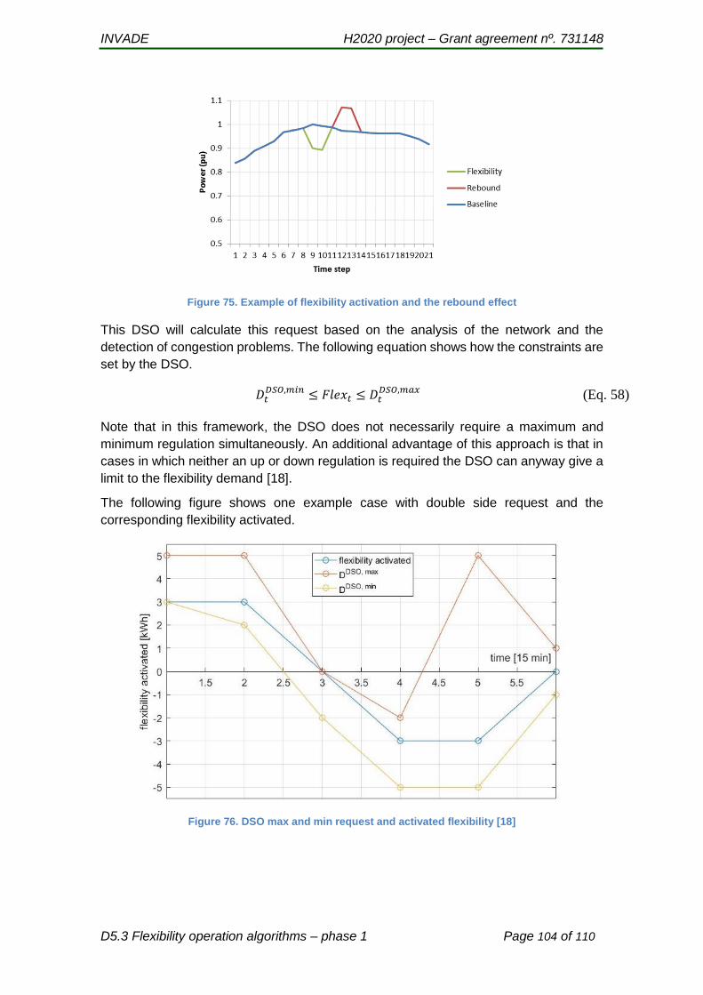
INVADE H2020 project – Grant agreement nº. 731148
D5.3 Flexibility operation algorithms – phase 1 Page 104 of 110
Figure 75. Example of flexibility activation and the rebound effect
This DSO will calculate this request based on the analysis of the network and the
detection of congestion problems. The following equation shows how the constraints are
set by the DSO.
Note that in this framework, the DSO does not necessarily require a maximum and
minimum regulation simultaneously. An additional advantage of this approach is that in
cases in which neither an up or down regulation is required the DSO can anyway give a
limit to the flexibility demand [18].
The following figure shows one example case with double side request and the
corresponding flexibility activated.
Figure 76. DSO max and min request and activated flexibility [18]
𝐷𝑡𝐷𝑆𝑂,𝑚𝑖𝑛 ≤ 𝐹𝑙𝑒𝑥𝑡 ≤ 𝐷𝑡
𝐷𝑆𝑂,𝑚𝑎𝑥 (Eq. 58)
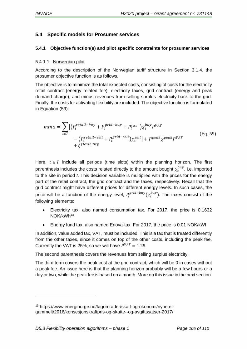
INVADE H2020 project – Grant agreement nº. 731148
D5.3 Flexibility operation algorithms – phase 1 Page 105 of 110
5.4 Specific models for Prosumer services
5.4.1 Objective function(s) and pilot specific constraints for prosumer services
5.4.1.1 Norwegian pilot
According to the description of the Norwegian tariff structure in Section 3.1.4, the
prosumer objective function is as follows.
The objective is to minimize the total expected costs, consisting of costs for the electricity
retail contract (energy related fee), electricity taxes, grid contract (energy and peak
demand charge), and minus revenues from selling surplus electricity back to the grid.
Finally, the costs for activating flexibility are included. The objective function is formulated
in Equation (59):
Here, 𝑡 ∈ 𝑇 include all periods (time slots) within the planning horizon. The first
parenthesis includes the costs related directly to the amount bought 𝜒𝑡𝑏𝑢𝑦
, i.e. imported
to the site in period t. This decision variable is multiplied with the prices for the energy
part of the retail contract, the grid contract and the taxes, respectively. Recall that the
grid contract might have different prices for different energy levels. In such cases, the
price will be a function of the energy level, 𝑃𝑡𝑔𝑟𝑖𝑑−𝑏𝑢𝑦
(𝜒𝑡𝑏𝑢𝑦
). The taxes consist of the
following elements:
Electricity tax, also named consumption tax. For 2017, the price is 0.1632
NOK/kWh13
Energy fund tax, also named Enova-tax. For 2017, the price is 0.01 NOK/kWh
In addition, value added tax, VAT, must be included. This is a tax that is treated differently
from the other taxes, since it comes on top of the other costs, including the peak fee.
Currently the VAT is 25%, so we will have 𝑃𝑉𝐴𝑇 = 1.25.
The second parenthesis covers the revenues from selling surplus electricity.
The third term covers the peak cost at the grid contract, which will be 0 in cases without
a peak fee. An issue here is that the planning horizon probably will be a few hours or a
day or two, while the peak fee is based on a month. More on this issue in the next section.
13 https://www.energinorge.no/fagomrader/skatt-og-okonomi/nyheter-gammelt/2016/konsesjonskraftpris-og-skatte--og-avgiftssatser-2017/
𝑚𝑖𝑛 z = ∑[(𝑃𝑡𝑟𝑒𝑡𝑎𝑖𝑙−𝑏𝑢𝑦
+ 𝑃𝑡𝑔𝑟𝑖𝑑−𝑏𝑢𝑦
+ 𝑃𝑡𝑡𝑎𝑥 )𝜒𝑡
𝑏𝑢𝑦𝑃𝑉𝐴𝑇
𝑡∈𝑇
− (𝑃𝑡𝑟𝑒𝑡𝑎𝑖𝑙−𝑠𝑒𝑙𝑙 + 𝑃𝑡
𝑔𝑟𝑖𝑑−𝑠𝑒𝑙𝑙)𝜒𝑡
𝑠𝑒𝑙𝑙] + 𝑃𝑝𝑒𝑎𝑘𝜒𝑝𝑒𝑎𝑘𝑃𝑉𝐴𝑇
+ 𝜁𝑓𝑙𝑒𝑥𝑖𝑏𝑖𝑙𝑖𝑡𝑦
(Eq. 59)

INVADE H2020 project – Grant agreement nº. 731148
D5.3 Flexibility operation algorithms – phase 1 Page 106 of 110
The last part of the objective function is the cost for utilizing the flexibility from the internal
resources. This cost may cover a wide variety of costs that must be further discussed,
but some examples are:
Loss of comfort from shifting or curtailing loads
Disutility from delaying EV charging or even from not meeting the charging
demand
Battery aging
The contribution to 𝜁𝑓𝑙𝑒𝑥𝑖𝑏𝑖𝑙𝑖𝑡𝑦 has been described under each section for the different
resource types.
5.4.1.2 Dutch pilot
The objective functions for the different Dutch pilot sites will be formulated at a later
stage, after further discussions with Elaad and GreenFlux.
5.4.1.3 Bulgarian pilot
According to the pilot specification in section Error! Reference source not found., the
ain objective is to shift as much as possible of the load from the peak-load hours to the
off-peak load hors. This can be formulated as:
An alternative formulation is to maximize the up-regulation in the peak load hours:
Notice that this formulation only covers batteries and flexible loads. Also notice that it
presupposes that the battery has no baseline schedule. If other resource types, like EV
charging points are added, or batteries have a baseline schedule, the formulation must
be changed.
5.4.1.4 Spanish pilot
Not applicable in phase 1.
𝑚𝑖𝑛 z𝐵𝑢𝑙𝑔1 = ∑ 𝜒𝑡𝑏𝑢𝑦
20
𝑡=9
(Eq. 60)
𝑚𝑎𝑥 z𝐵𝑢𝑙𝑔2 = ∑ (∑ 𝜎𝑏,𝑡𝐵,𝑜𝑢𝑡
𝑏∈𝐵
− ∑ 𝜎𝑏,𝑡𝐵,𝑖𝑛
𝑏∈𝐵
+ ∑ ( 𝑊𝑙,𝑡 − 𝜔𝑙,𝑡 )
𝑙∈𝐿
)
20
𝑡=9
(Eq. 61)
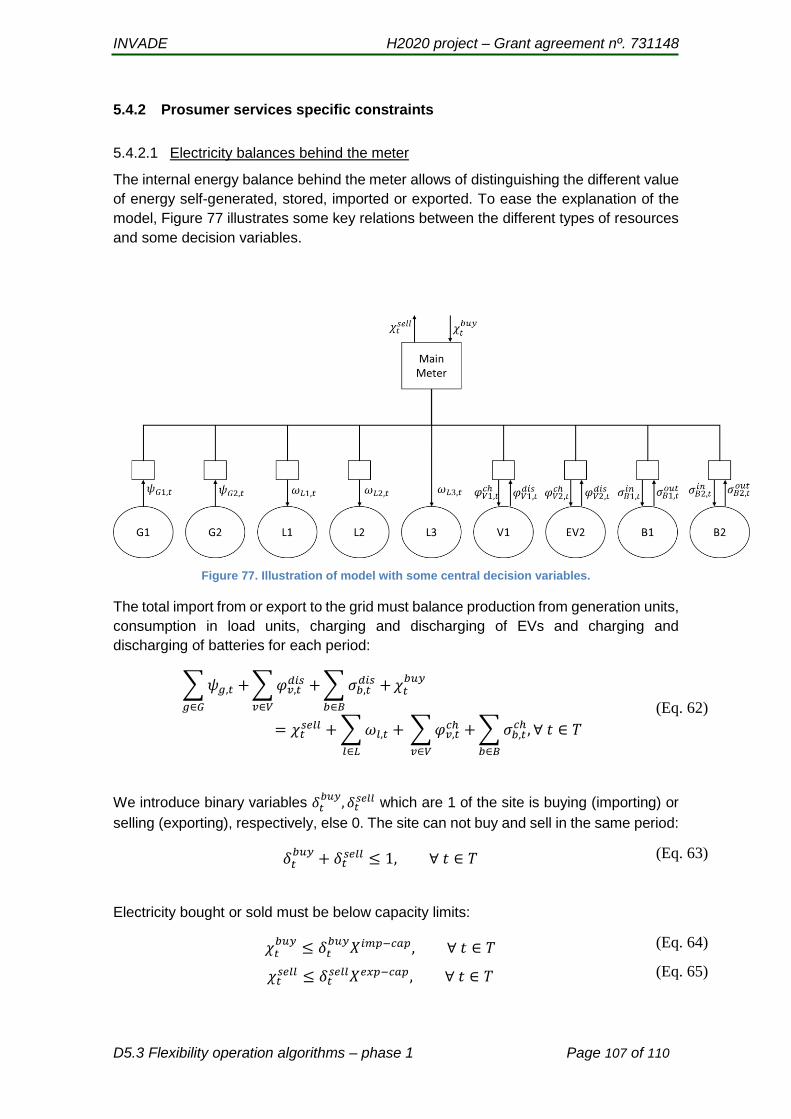
INVADE H2020 project – Grant agreement nº. 731148
D5.3 Flexibility operation algorithms – phase 1 Page 107 of 110
5.4.2 Prosumer services specific constraints
5.4.2.1 Electricity balances behind the meter
The internal energy balance behind the meter allows of distinguishing the different value
of energy self-generated, stored, imported or exported. To ease the explanation of the
model, Figure 77 illustrates some key relations between the different types of resources
and some decision variables.
Figure 77. Illustration of model with some central decision variables.
The total import from or export to the grid must balance production from generation units,
consumption in load units, charging and discharging of EVs and charging and
discharging of batteries for each period:
We introduce binary variables 𝛿𝑡𝑏𝑢𝑦
, 𝛿𝑡𝑠𝑒𝑙𝑙 which are 1 of the site is buying (importing) or
selling (exporting), respectively, else 0. The site can not buy and sell in the same period:
Electricity bought or sold must be below capacity limits:
∑ 𝜓𝑔,𝑡 +
𝑔∈𝐺
∑ 𝜑𝑣,𝑡𝑑𝑖𝑠 +
𝑣∈𝑉
∑ 𝜎𝑏,𝑡𝑑𝑖𝑠 +
𝑏∈𝐵
𝜒𝑡𝑏𝑢𝑦
= 𝜒𝑡𝑠𝑒𝑙𝑙 + ∑ 𝜔𝑙,𝑡 +
𝑙∈𝐿
∑ 𝜑𝑣,𝑡𝑐ℎ +
𝑣∈𝑉
∑ 𝜎𝑏,𝑡𝑐ℎ,
𝑏∈𝐵
∀ 𝑡 ∈ 𝑇
(Eq. 62)
𝛿𝑡𝑏𝑢𝑦
+ 𝛿𝑡𝑠𝑒𝑙𝑙 ≤ 1, ∀ 𝑡 ∈ 𝑇 (Eq. 63)
𝜒𝑡𝑏𝑢𝑦
≤ 𝛿𝑡𝑏𝑢𝑦
𝑋𝑖𝑚𝑝−𝑐𝑎𝑝, ∀ 𝑡 ∈ 𝑇 (Eq. 64)
𝜒𝑡𝑠𝑒𝑙𝑙 ≤ 𝛿𝑡
𝑠𝑒𝑙𝑙𝑋𝑒𝑥𝑝−𝑐𝑎𝑝, ∀ 𝑡 ∈ 𝑇 (Eq. 65)

INVADE H2020 project – Grant agreement nº. 731148
D5.3 Flexibility operation algorithms – phase 1 Page 108 of 110
Notice that in cases with a kWmax value that is physical, 𝑋𝑖𝑚𝑝−𝑐𝑎𝑝 must be set to this
value. In some cases this value might be dynamic (?). Then we need to introduce a time
index.
Also notice that in some cases 𝑋𝑒𝑥𝑝−𝑐𝑎𝑝 will be a physical limit, while in others it might
be a commercial or regulatory limit. The last is the case with the plus-customer
arrangement in Norway. Then we will have 𝑋𝑒𝑥𝑝−𝑐𝑎𝑝 = 100 kW. In Bulgaria, where there
is no arrangement for selling electricity back to the grid, we will have 𝑋𝑒𝑥𝑝−𝑐𝑎𝑝 = 0 kW.
In cases with subscribed power, the cost of the energy part of the grid fee 𝑃𝑡𝑔𝑟𝑖𝑑−𝑏𝑢𝑦
will
be dependent on the consumption level 𝜒𝑡𝑏𝑢𝑦
. Assume that there will be two prices,
𝑃𝑡𝑔𝑟𝑖𝑑−𝑏𝑢𝑦−𝑙𝑜𝑤
and 𝑃𝑡𝑔𝑟𝑖𝑑−𝑏𝑢𝑦−ℎ𝑖𝑔ℎ
, where the low price is valid for periods where the
bought volume is below a threshold value. This can be formulated:
𝑃𝑡𝑔𝑟𝑖𝑑−𝑏𝑢𝑦
= 𝑃𝑡𝑔𝑟𝑖𝑑−𝑏𝑢𝑦−𝑙𝑜𝑤
, 𝑖𝑓 𝜒𝑡𝑏𝑢𝑦
≤ 𝑋𝑠𝑢𝑏𝑠𝑐𝑟𝑖𝑏𝑒𝑑 (Eq. 66)
𝑃𝑡𝑔𝑟𝑖𝑑−𝑏𝑢𝑦
= 𝑃𝑡𝑔𝑟𝑖𝑑−𝑏𝑢𝑦−ℎ𝑖𝑔ℎ
, 𝑖𝑓 𝜒𝑡𝑏𝑢𝑦
> 𝑋𝑠𝑢𝑏𝑠𝑐𝑟𝑖𝑏𝑒𝑑 (Eq. 67)
INVADE H2020 project – Grant agreement nº. 731148
D5.3 Flexibility operation algorithms – phase 1 Page 109 of 110
References
[1] P. Olivella-Rosell et al., “Optimization problem for meeting distribution system operator requests in local flexibility markets with distributed energy resources,” Appl. Energy, vol. 210, no. Supplement C, pp. 881–895, Jan. 2018.
[2] Eurelectric, “Flexibility and Aggregation Requirements for their interaction in the market,” Eurelectric, 2014.
[3] S. O. Ottesen and A. Tomasgard, “A stochastic model for scheduling energy flexibility in buildings,” Energy, vol. 88, pp. 364–376, Aug. 2015.
[4] M. Schimpe et al., “Energy efficiency evaluation of a stationary lithium-ion battery container storage system via electro-thermal modeling and detailed component analysis,” Appl. Energy, vol. 210, no. Supplement C, pp. 211–229, Jan. 2018.
[5] J. Wang, Y. Shi, K. Fang, Y. Zhou, and Y. Li, “A Robust Optimization Strategy for Domestic Electric Water Heater Load Scheduling under Uncertainties,” Appl. Sci., vol. 7, no. 11, p. 1136, Nov. 2017.
[6] N. Lu, D. P. Chassin, and S. E. Widergren, “Modeling uncertainties in aggregated thermostatically controlled loads using a State queueing model,” IEEE Trans. Power Syst., vol. 20, no. 2, pp. 725–733, May 2005.
[7] V. Lakshmanan, M. Marinelli, A. M. Kosek, P. B. Nørgård, and H. W. Bindner, “Impact of thermostatically controlled loads’ demand response activation on aggregated power: A field experiment,” Energy, vol. 94, no. Supplement C, pp. 705–714, Jan. 2016.
[8] P. Pinson, H. Madsen, H. A. Nielsen, G. Papaefthymiou, and B. Klöckl, “From probabilistic forecasts to statistical scenarios of short-term wind power production,” Wind Energy, vol. 12, no. 1, pp. 51–62, Jan. 2009.
[9] R. Ramakrishna, A. Scaglione, and V. Vittal, “A Stochastic Model for Short-Term Probabilistic Forecast of Solar Photo-Voltaic Power,” ArXiv170605445 Stat, Jun. 2017.
[10] D. Bertsimas, D. Brown, and C. Caramanis, “Theory and Applications of Robust Optimization,” SIAM Rev., vol. 53, no. 3, pp. 464–501, Jan. 2011.
[11] A. Hussain, V.-H. Bui, and H.-M. Kim, “Robust Optimization-Based Scheduling of Multi-Microgrids Considering Uncertainties,” Energies, vol. 9, no. 4, p. 278, Apr. 2016.
[12] “Optimization Online - A Stochastic MPC Framework for Stationary Battery Systems.” [Online]. Available: http://www.optimization-online.org/DB_HTML/2017/05/6044.html. [Accessed: 05-Dec-2017].
[13] P. Malysz, S. Sirouspour, and A. Emadi, “An Optimal Energy Storage Control Strategy for Grid-connected Microgrids,” IEEE Trans. Smart Grid, vol. 5, no. 4, pp. 1785–1796, Jul. 2014.
[14] E. L. Ratnam and S. R. Weller, “Receding horizon optimization-based approaches to managing supply voltages and power flows in a distribution grid with battery storage co-located with solar PV,” Appl. Energy, Sep. 2017.
[15] R. Palma-Behnke et al., “A Microgrid Energy Management System Based on the Rolling Horizon Strategy,” IEEE Trans. Smart Grid, vol. 4, no. 2, pp. 996–1006, Jun. 2013.

INVADE H2020 project – Grant agreement nº. 731148
D5.3 Flexibility operation algorithms – phase 1 Page 110 of 110
[16] K. Baker, G. Hug, and X. Li, “Energy Storage Sizing Taking Into Account Forecast Uncertainties and Receding Horizon Operation,” IEEE Trans. Sustain. Energy, vol. 8, no. 1, pp. 331–340, Jan. 2017.
[17] P. Malysz, S. Sirouspour, and A. Emadi, “MILP-based rolling horizon control for microgrids with battery storage,” in IECON 2013 - 39th Annual Conference of the IEEE Industrial Electronics Society, 2013, pp. 2099–2104.
[18] D. Fraizzoli, “Methodology to estimate the flexibility potential of an aggregator’s portfolio in a residential distribution grid,” Sep. 2017.
INVADE H2020 project – Grant nº 731148
This project has received funding from the European Union’s Horizon 2020 Research and Innovation programme under Grant Agreement No 731148.
Smart system of renewable energy storage based on INtegrated EVs and
bAtteries to empower mobile, Distributed and centralised Energy storage
in the distribution grid
Deliverable nº: D5.3-part 2 of 2
Deliverable name: Placement and Sizing of Batteries in Low and Medium Voltage Grids
Version: 1.0
Release date: 20/12/2017
Dissemination level: Public (Public, Confidential)
Status: Submitted (Draft, Peer-reviewed, Submitted, Approved)
Authors: Pedro Crespo del Granado, Sigurd Bjarghov, Venkatachalam Lakshmanan, Jamshid Aghaei, Magnus Korpås and Hossein Farahmand – NTNU
Pol Olivella-Rosell – UPC

INVADE H2020 project – Grant nº 731148
D5.3- Placement and Sizing of Batteries in Low and Medium Voltage Grids Page 2 of 39
Document history:
Version Date of issue Content and changes Edited by
0.1 26/10/2017 First outline draft version P. Crespo del Granado
0.2 03/11/2017 Updated outline
V. Lakshmanan, P. Crespo del Granado, S. Bjarghov, J. Aghaei and H. Farahmand
0.3 23/11/2017 Introduction description and Chapter 3
V. Lakshmanan, J. Aghaei and H. Farahmand
0.4 17/11/2017 Removed battery chapter (now in first document)
P. Crespo del Granado and H. Farahmand
0.5 23/11/2017 Introduction description and Chapter 3
V. Lakshmanan, J. Aghaei and H. Farahmand
0.6 27/11/2017
Completed all chapters except ch. 2 and sec 3.3.1-2; Updates in Simplified model in Sizing and Siting problems
P. Crespo del Granado, J. Aghaei and H. Farahmand
0.7 30/11/2017 Comments on quality check M. Korpås
0.8 1/12/2017
New updates in all chapters, sub-chapter 1.2 is added, planning model for DSO is updated, Chapter 3 is updated, sub-chapter 3.3.1 is completed
V. Lakshmanan, P. Crespo del Granado, S. Bjarghov, J. Aghaei and H. Farahmand
0.9 5/12/2017 Final edit
V. Lakshmanan, P. Crespo del Granado, S. Bjarghov, J. Aghaei and H. Farahmand
1.0 20/12/2017 Version ready for approval, updated with comments from peer-reviewers
V. Lakshmanan, P. Crespo del Granado, S. Bjarghov, J. Aghaei and H. Farahmand
Peer reviewed by:
Partner Reviewer
SmartIO Jayaprakash Rajasekharan
GreenFlux Michel Bayings

INVADE H2020 project – Grant nº 731148
D5.3- Placement and Sizing of Batteries in Low and Medium Voltage Grids Page 3 of 39
Deliverable beneficiaries:
WP / Task
WP5 / Task 5.3 and 5.4
WP8 / Task T8.3
WP10

INVADE H2020 project – Grant nº 731148
D5.3- Placement and Sizing of Batteries in Low and Medium Voltage Grids Page 4 of 39
Table of contents
Executive summary .................................................................................................... 7
Introduction .......................................................................................................... 8
1.1 INVADE Flexibility Services: siting and sizing considerations 8
1.2 Siting and sizing consideration for pilots 10
Simplified planning model in Sizing and Siting problems ............................... 11
2.1 A planning algorithm from the prosumer perspective (Sizing problem) 12
2.2 A planning algorithm from the DSO perspective ( Sizing and Siting problem) 13
2.3 Bi-level Optimization Model 14
2.4 Simple investment model from the prosumer point of view 15
2.4.1 Master Problem 18
2.4.2 Sequential Sub-problem 18
2.5 Simple investment model from DSO point of view 19
2.5.1 Representation of multi-period AC optimal power flows
constraints 21
Pilots and illustrative sizing examples for prosumers..................................... 24
3.1 Flexibility needed due to kWmax and self-balancing 25
3.2 INVADE pilots data collection for simplified model 26
3.2.1 INVADE pilot: Homes in the Netherlands 26
3.2.2 INVADE pilot: Hotel in Albena, Bulgaria 27
3.2.3 Data sets used, assumptions and limitations 28
3.3 Implementation and illustrative preliminary results 30
3.3.1 Battery-PV sizing for houses in Netherlands 30
3.3.2 Battery-PV sizing for Albena 33
Concluding Remarks .......................................................................................... 34

INVADE H2020 project – Grant nº 731148
D5.3- Placement and Sizing of Batteries in Low and Medium Voltage Grids Page 5 of 39
References ................................................................................................................ 35
Appendix I 37
The Mixed Integer Linear Programing (MILP) Model 37

INVADE H2020 project – Grant nº 731148
D5.3- Placement and Sizing of Batteries in Low and Medium Voltage Grids Page 6 of 39
Abbreviations and Acronyms
Acronym Description
AC Alternating Current
BD Benders Decomposition
BRP Balancing Responsible Party
DER Distributed Energy Resources
DG Distributed Generation
DR Demand Response
DSM Demand Side Management
DSO Distribution System Operator
EV Electric Vehicle
FO Flexibility Operator
FR Flexibility Reserve
LV Low voltage
MIP Mixed Integer Problem
MILP Mixed Integer Linear Programing
NLP Nonlinear Programming
NPV Net Present Value
OPF Optimal Power Flow
PV Photovoltaics
RES Renewable Energy Sources
SOC State Of Charge
ToU Time of Use

INVADE H2020 project – Grant nº 731148
D5.3- Placement and Sizing of Batteries in Low and Medium Voltage Grids Page 7 of 39
Executive summary
The deployment of batteries in the distribution network can provide an array of flexibility
services to integrate renewable energy sources (RES) and improve grid operation in
general. Capturing and quantifying the value of storage for different flexibility services
require models that can represent the technological detail of battery-RES-load
interactions to provide scheduling strategies for real-time operations. For this purpose,
deliverable 5.3 focuses on models and algorithms for: 1) battery capacity and location
planning, 2) daily operations and 3) real-time control.
Battery sizing has different implications and benefits for distribution system operators
(DSO), balance responsible parties (BRPs) and prosumers, respectively. In this
document, the issues and approaches related to siting, capacity planning and investment
analysis are discussed. A simplified planning strategy that leverages the control
strategies of battery charging and discharging to find the optimal location and size of
batteries in distribution system is presented. A general planning algorithm from both
prosumer and DSO perspectives are presented. This is complemented with illustrative
examples on battery-PV sizing analyses for prosumers. The simplified sizing methods
are tested for the pilots in Albena Hotel (Bulgaria) and small houses in the Netherlands.
According to D 4.2 [1], in order to implement flexibility services progressively, the
INVADE implementation has been divided in two phases. Here, phase 1 includes the
implementation of prosumer services for ToU optimization, kWmax control and Self-
balancing plus the DSO service congestion management. Note that in a separate
document (D5.3-Flexibility operations algorithms-phase 1), the details of the simplified
model intended for phase 1 are fully described. This model will be implemented in the
platform of the INVADE flexibility cloud as part of T8.3.

INVADE H2020 project – Grant nº 731148
D5.3- Placement and Sizing of Batteries in Low and Medium Voltage Grids Page 8 of 39
Introduction
INVADE deliverable D5.3 “Simplified Battery operation and control algorithm” is divided
into two documents: 5.3-first part and 5.3-second part. D5.3-first part presents design
and program the flexibility management operation algorithm as part of 5.4, whereas the
D5.3-second part presents energy storage units allocation/positioning and sizing
algorithm as part of task 5.3. This document describes simplified models and methods
for siting and sizing of batteries. In this deliverable, a simplified model means that the
representation of batteries are assumed to have linear charging and discharging power
characteristics, which is irrespective of its state of charge (SOC). The charge/discharge
efficiency of the battery are assumed to be constant and not depend of their SOC, cell
operating temperature and charging/discharge power. The battery and EV models will
be extended in WP6 (T6.4 “Advanced Battery techno-economic model”) by including
more technical parameters and economics of second life batteries. Another example of
simplification is that adjustable loads like thermal loads are modelled with an assumption
of linear relation between their energy consumption and temperature.
1.1 INVADE Flexibility Services: siting and sizing considerations
Proper sizing of the flexibility resource (i.e. batteries) is important for investment planning
decisions and siting is key for its effective operation. The siting and sizing decision differs
based on the flexibility services required and the user cases (mobile, distributed,
centralized and hybrid). INVADE defined possible flexibility services for prosumers,
DSOs and BRPs. In this document, we focus on the prosumer and DSO perspectives.
There are three flexibility services in consideration for prosumers. First, the Time of Use
(ToU) flexibility service uses a battery for the effective utilization of local RES production
and to avoid high tariffs by managing high peak demand. That is, the prosumer demand
is adjusted in such a way (due to battery presence) that the consumption from the grid
at peak hours will be moved to off-peak hours. In this case, the battery sizing algorithm
will decide the battery capacity by considering the demand and local RES production.
The second flexibility service from the prosumer perspective is kWmax control. This
service limits the maximum amount of power imported or exported to the grid at any time
at the prosumer level. If the kWmax is linked to a physical limitation, it becomes an
additional constraint for optimization problem on both battery sizing and load shifting on
day-to-day operation. However, if it is linked to a tariff structure, it can model as a penalty

INVADE H2020 project – Grant nº 731148
D5.3- Placement and Sizing of Batteries in Low and Medium Voltage Grids Page 9 of 39
for maximum purchase. The third flexibility service is self-balancing in which the battery
supports possible zero import and export of energy from the grid. A proper battery size
would allow to optimally balancing demand and local RES production. The detailed
operation strategy for day-to-day operation for prosumer services are given in the 5.3
first document. In D5.3 second document, through a simplified operational model, we
illustrate and test how different battery sizes affects the integration of PV capacity under
kWmax control restrictions. This illustrative example is applied to the pilots in The
Netherlands and Bulgaria (see chapter 3). Note that for prosumers, only the sizing part
of the problem is relevant there is usually one single location: the prosumer and its on-
site RES.
Regarding the DSO perspective, there are three flexibility services considered: 1)
congestion management, 2) voltage/reactive power control and 3) controlled islanding.
D5.3 focuses on congestion management since it has be considered as a DSO service
included in phase 1 of the INVADE implementation. For this flexibility service, the DSO
sends requests to a flexibility operator (FO) to activate or call for available flexibility
sources. Then, the FO schedules the batteries charge/discharge operations at the
neighbourhood and prosumer levels to meet the requirement of the DSO. For example,
the storage at the neighbourhood level could be one large array of battery bank located
near the substation or multiple arrays of battery banks located at different nodes. In this
situation, battery siting and sizing plays an important role specially to increase RES
penetration in the distribution network without violating the network power flow limits. The
siting of batteries might be constrained by the electric distribution network topology and
their power flow capacities. Poor siting of batteries may bring underutilization of the
resources as well as they could create new voltage and congestion problems in the
distribution network. Therefore conducting optimal power flow (OPF) analyses for the
different siting options in the distribution network is essential to determine the most
beneficial locations. The Optimal Power Flow (OPF) problem for alternating current (AC)
circuits concerns the problem of determining the voltage magnitude, the voltage angle,
the real power injection, the reactive power injection at each given grid node to minimize
a cost function. Typical objective functions used in OPF problems are the total
generation. The constraints for OPF include (i) the AC power flow constraints, (ii) bounds
on power generation, (iii) bounds on bus voltage magnitudes, (iv) bounds on thermal
losses, and (v) limits on power transfer on lines. Unlike the transmission systems, the
nodal voltages of the distribution systems are influenced by the active and reactive power
flows and their directions. Moreover, it is the responsibility of the distribution system
operator to maintain the voltages within the allowable limits. On the other hand, if the

INVADE H2020 project – Grant nº 731148
D5.3- Placement and Sizing of Batteries in Low and Medium Voltage Grids Page 10 of 39
battery storage is included due to the multi-period time dimension introduced by the
battery storage, a few consecutive and coupled optimal power flows are needed to
simulate the charge/discharge battery cycle over given operating horizon [2].
The siting problem, using multi-period OPF is a mixed nonlinear integer program due to
nonlinearity of AC power flow equations, which might become computationally
intractable for large-scale optimization problems [3-6].
1.2 Siting and sizing consideration for pilots
There are five pilots planned in the project INVADE as described in D4.2[1]. The details
of the different pilots and their association with the different DSO and Prosumer services
are detailed here.
1) Norwegian pilot: The Norwegian pilot will demonstrate 3 different prosumer
service. They are ToU optimization, kWmax control and Self-balancing. For
Norwegian pilot, the problem is more focused around the sizing of storage rather
than siting.
2) Dutch pilot: The Dutch pilot has both DSO and prosumer service in their
demonstration. This pilot will demonstrate congestion management and voltage
/ reactive control as DSO services and ToU optimization, kWmax control and
Self-balancing as prosumer services. Both DSO and prosumer services of this
pilot are provided from the prosumer flexibility and mobile batteries of EV.
Therefore, sizing is the primary problem and siting problem will focus on OPF for
providing DSO services.
3) Bulgarian pilot: The Bulgarian pilot is a large prosumer case to demonstrate 3
prosumer services and the 4th prosumer service “Controlled islanding” maybe
included based on the feasibility at the time of implementation. Therefore, the
Bulgarian pilot exposes the sizing problem only.
4) German pilot: The 3 prosumer services ToU optimization, kWmax control and
Self-balancing and the DSO service congestion management are planned for the
German pilot. The source of flexibility for this pilot is from both distributed and
centralized storage. Therefore, both siting and sizing are equally important for
German pilot.
5) Spanish pilot: The Spanish pilot primarily demonstrate the DSO services namely
congestion management with centralized storage. Therefore, the siting problem
is as important as the sizing problem.

INVADE H2020 project – Grant nº 731148
D5.3- Placement and Sizing of Batteries in Low and Medium Voltage Grids Page 11 of 39
Simplified planning model in Sizing and Siting
problems
The main objective of this section is to develop a simplified planning strategy that
leverages the control strategies of battery charging and discharging acting on control
horizons to find the optimal location and size of batteries in distribution system. The
planning strategy links the operational domain with the planning domain to find an
optimal investment decision.
The methods to be used is based on calculating the Net Present Value (NPV) of a battery
investment, which is the difference between the present value of cash inflows and the
present value of cash outflows. For a battery investment (and installation) at the start of
the analysis period is cash outflows and operational net benefits are deemed as cash
inflow. Hence, the NPV is in its simplest form given as Eq. (2.1) [7].
𝑁𝑃𝑉(𝑃𝑟𝑎𝑡 , 𝐸𝑟𝑎𝑡) = [∑𝑅(𝑃𝑟𝑎𝑡,𝐸𝑟𝑎𝑡,𝑛)−𝑂(𝑃𝑟𝑎𝑡,𝐸𝑟𝑎𝑡,𝑛)
(1+𝑟)𝑛] − 𝐶(𝑃𝑟𝑎𝑡 , 𝐸𝑟𝑎𝑡)
𝑁𝑛=1 (Eq. 2.1)
Where, R is the annual revenue, O is the annual operational costs and C is the equivalent
annual installation cost, which is dependent of the rated power and energy storage
capacity of the battery. By assuming that each year is equal and neglecting maintenance
costs of the battery, we obtain
𝑁𝑃𝑉(𝑃𝑟𝑎𝑡 , 𝐸𝑟𝑎𝑡) = [𝑅(𝑃𝑟𝑎𝑡 , 𝐸𝑟𝑎𝑡) − 𝑂(𝑃𝑟𝑎𝑡 , 𝐸𝑟𝑎𝑡 , 𝑛)] − 𝛼𝑁,𝑟 ∙ 𝐶(𝑃𝑟𝑎𝑡 , 𝐸𝑟𝑎𝑡) (Eq. 2.2)
Where, α is the annuity factor1. The annual revenue can be expressed as Eq. (2.3).
𝑅(𝑃𝑟𝑎𝑡 , 𝐸𝑟𝑎𝑡) = ∑ 𝑅𝑜𝑝(𝑃𝑟𝑎𝑡 , 𝐸𝑟𝑎𝑡 , 𝑡)𝑇𝑡=1 + 𝑅𝑓𝑖𝑥𝑒𝑑(𝑃𝑟𝑎𝑡 , 𝐸𝑟𝑎𝑡) (Eq. 2.3)
The resolution of the time step t depends on the market conditions and technical
requirements for activation of services. The time step size t can, e.g., be one minute, 15
minutes or 1 hour. In this document, we use several terminologies about planning
horizon, and we have explain them in the following bullets:
The shortest planning horizon is the operational planning horizon represented by
T in Eq. (2.3), e.g. 6 hours, 12 hours, or 24 hours
1 𝛼𝑛,𝑟 =𝑟
1−(1+𝑟)−𝑛 where, r is discount rate

INVADE H2020 project – Grant nº 731148
D5.3- Placement and Sizing of Batteries in Low and Medium Voltage Grids Page 12 of 39
The medium planning horizon is related to how many operational situations we
will base our investment decision on. This can be one year (or more, depending
on long-term uncertainties regarding spot prices, load development etc). Usually
we use “one representative year”, but a realistic model should cover more
The long-term planning horizon is at least as long as the economic lifetime of the
investment option, i.e. the battery in our case represented by N in Eq. (2.1)
In general, the economic optimal size of the battery is the size that maximizes the NPV,
taking into account all technical constraints and market possibilities. This is a trade-off
between operational benefit – given the battery’s technical capabilities - and investment
cost.
2.1 A planning algorithm from the prosumer perspective (Sizing
problem)
We introduce a planning algorithm from different grid user perspectives. First, we focus
on the prosumer perspective, where the operating objective function refers to the
electricity bill minimization problem. In this problem, the primary objective is to find the
optimal sizing of the battery that maximizes the NPV. Hence, R is operational cost
savings due to flexibility that the battery will provide to the prosumer compared to a
system without the battery. The annual revenue is the sum of revenues obtained from
prosumer services. The prosumer model is similar to the model illustrated in D5.3-first
part, “Design and program the flexibility management operation algorithm”. The
prosumer is equipped with the main meter, which is placed at the border of connection
point to the network, and may have sub meters (at the resource level). The prosumer
can have one or several flexibility resources as following:
Generator resources
Load resources
Electric vehicles (EVs)
The detailed model of the above flexibility sources is presented in D5.3-first part. The
model is shown in Figure 1.
Figure 1
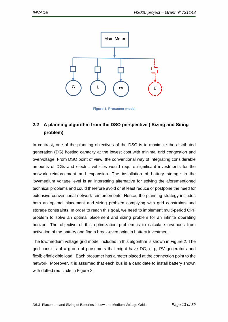
INVADE H2020 project – Grant nº 731148
D5.3- Placement and Sizing of Batteries in Low and Medium Voltage Grids Page 13 of 39
Figure 1. Prosumer model
2.2 A planning algorithm from the DSO perspective ( Sizing and Siting
problem)
In contrast, one of the planning objectives of the DSO is to maximize the distributed
generation (DG) hosting capacity at the lowest cost with minimal grid congestion and
overvoltage. From DSO point of view, the conventional way of integrating considerable
amounts of DGs and electric vehicles would require significant investments for the
network reinforcement and expansion. The installation of battery storage in the
low/medium voltage level is an interesting alternative for solving the aforementioned
technical problems and could therefore avoid or at least reduce or postpone the need for
extensive conventional network reinforcements. Hence, the planning strategy includes
both an optimal placement and sizing problem complying with grid constraints and
storage constraints. In order to reach this goal, we need to implement multi-period OPF
problem to solve an optimal placement and sizing problem for an infinite operating
horizon. The objective of this optimization problem is to calculate revenues from
activation of the battery and find a break-even point in battery investment.
The low/medium voltage grid model included in this algorithm is shown in Figure 2. The
grid consists of a group of prosumers that might have DG, e.g., PV generators and
flexible/inflexible load. Each prosumer has a meter placed at the connection point to the
network. Moreover, it is assumed that each bus is a candidate to install battery shown
with dotted red circle in Figure 2.
Main Meter
G L EV B
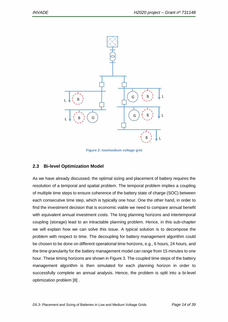
INVADE H2020 project – Grant nº 731148
D5.3- Placement and Sizing of Batteries in Low and Medium Voltage Grids Page 14 of 39
Figure 2: low/medium voltage grid
2.3 Bi-level Optimization Model
As we have already discussed, the optimal sizing and placement of battery requires the
resolution of a temporal and spatial problem. The temporal problem implies a coupling
of multiple time steps to ensure coherence of the battery state of charge (SOC) between
each consecutive time step, which is typically one hour. One the other hand, in order to
find the investment decision that is economic viable we need to compare annual benefit
with equivalent annual investment costs. The long planning horizons and intertemporal
coupling (storage) lead to an intractable planning problem. Hence, in this sub-chapter
we will explain how we can solve this issue. A typical solution is to decompose the
problem with respect to time. The decoupling for battery management algorithm could
be chosen to be done on different operational time horizons, e.g., 6 hours, 24 hours, and
the time granularity for the battery management model can range from 15 minutes to one
hour. These timing horizons are shown in Figure 3. The coupled time steps of the battery
management algorithm is then simulated for each planning horizon in order to
successfully complete an annual analysis. Hence, the problem is split into a bi-level
optimization problem [8] .
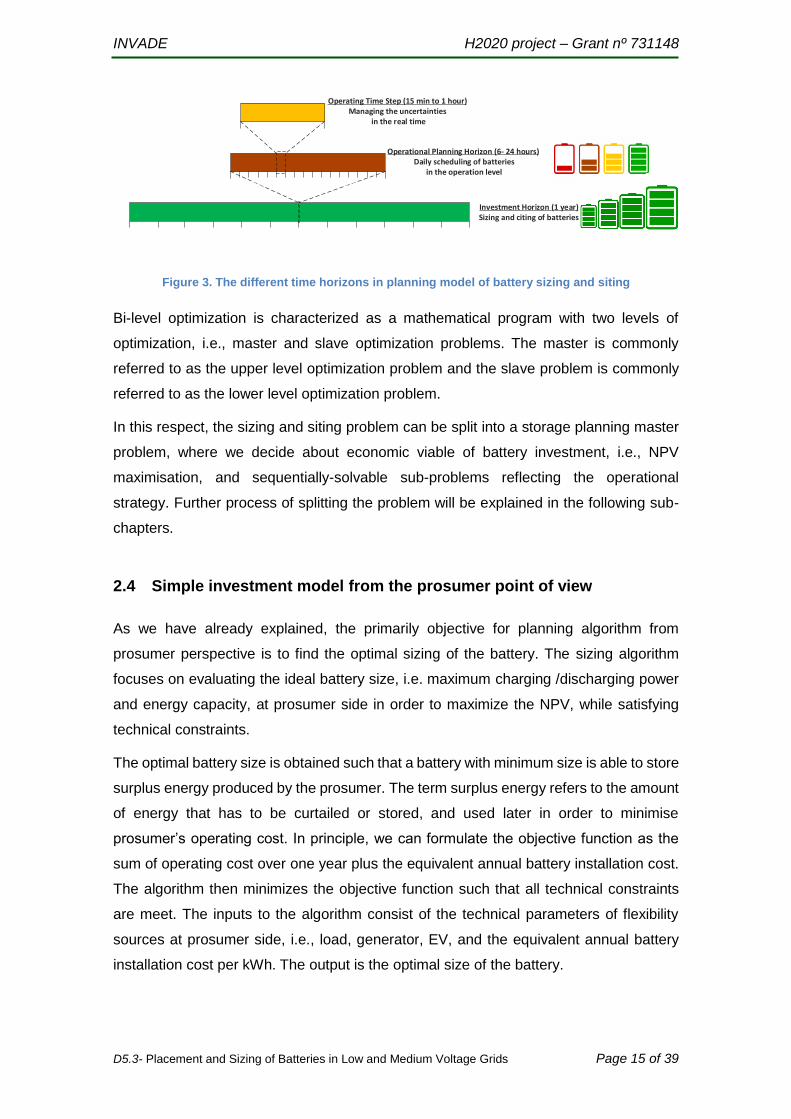
INVADE H2020 project – Grant nº 731148
D5.3- Placement and Sizing of Batteries in Low and Medium Voltage Grids Page 15 of 39
Figure 3. The different time horizons in planning model of battery sizing and siting
Bi-level optimization is characterized as a mathematical program with two levels of
optimization, i.e., master and slave optimization problems. The master is commonly
referred to as the upper level optimization problem and the slave problem is commonly
referred to as the lower level optimization problem.
In this respect, the sizing and siting problem can be split into a storage planning master
problem, where we decide about economic viable of battery investment, i.e., NPV
maximisation, and sequentially-solvable sub-problems reflecting the operational
strategy. Further process of splitting the problem will be explained in the following sub-
chapters.
2.4 Simple investment model from the prosumer point of view
As we have already explained, the primarily objective for planning algorithm from
prosumer perspective is to find the optimal sizing of the battery. The sizing algorithm
focuses on evaluating the ideal battery size, i.e. maximum charging /discharging power
and energy capacity, at prosumer side in order to maximize the NPV, while satisfying
technical constraints.
The optimal battery size is obtained such that a battery with minimum size is able to store
surplus energy produced by the prosumer. The term surplus energy refers to the amount
of energy that has to be curtailed or stored, and used later in order to minimise
prosumer’s operating cost. In principle, we can formulate the objective function as the
sum of operating cost over one year plus the equivalent annual battery installation cost.
The algorithm then minimizes the objective function such that all technical constraints
are meet. The inputs to the algorithm consist of the technical parameters of flexibility
sources at prosumer side, i.e., load, generator, EV, and the equivalent annual battery
installation cost per kWh. The output is the optimal size of the battery.
01.01.2017
31.12.201701.02.201701.03.2017 01.04.2017 01.05.2017 01.06.2017 01.07.2017 01.08.2017 01.09.2017 01.10.2017 01.11.2017 01.12.2017
07:00 23:5908:0009:0010:0011:0012:0013:0014:0015:0016:0017:0018:0019:0020:0021:0022:0023:00
12:00 13:00
Investment Horizon (1 year)Sizing and citing of batteries
Operational Planning Horizon (6- 24 hours) Daily scheduling of batteries
in the operation level
Operating Time Step (15 min to 1 hour)Managing the uncertainties
in the real time

INVADE H2020 project – Grant nº 731148
D5.3- Placement and Sizing of Batteries in Low and Medium Voltage Grids Page 16 of 39
A comprehensive formulation of flexibility operation algorithm has been presented in the
first document of this deliverable, i.e., “Flexibility operation algorithms – phase 1”. In the
first document, the objective function of flexibility operation has been presented from
different pilot perspectives. Typically, the objective for the prosumer is to minimize the
total expected operating costs, which in return may result in minimizing the peak load.
This can be presented by the Eq. (2.4).
min ( )
s.t.
(a) A
( ) A
( ) .
T
eq eq
in in
s s
J F
b
b b
c A b
(Eq. 2.4)
Where represents the amount of electricity bought/sold in the period t [kWh] or a basis
for calculation of the peak fee depending on the grid tariff structure. is representing
control variables of available flexibility services. Aeq and Ain
are matrices representing
technical constraints of procuring flexibility from the flexibility sources. sA is an
intertemporal battery coupling matrix, and is a battery energy capacity. In principle,
this constraint (Eq. 2.4-c) represents the coupling between the SOC on battery.
In order to find the economic optimal investment of the battery, the sizing algorithm can
be written in Eq. (2.5), where the battery is assume to be optimised over 24-h operational
horizon.
*
,
,
,
,
min ( ) .
s.t.
(a) A
( ) A
( ) .
d s
d D T
deq eq
d
din in
s s
J F c
b
b b
c A b
(Eq. 2.5)
Where, D is a total number of days in one year, and sc is the equivalent annual battery
installation cost. Consequently, the first term represents the sum of operating cost over
one year. The objective function consists of two terms representing:
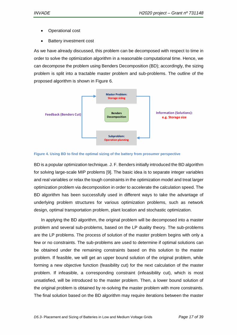
INVADE H2020 project – Grant nº 731148
D5.3- Placement and Sizing of Batteries in Low and Medium Voltage Grids Page 17 of 39
Operational cost
Battery investment cost
As we have already discussed, this problem can be decomposed with respect to time in
order to solve the optimization algorithm in a reasonable computational time. Hence, we
can decompose the problem using Benders Decomposition (BD); accordingly, the sizing
problem is split into a tractable master problem and sub-problems. The outline of the
proposed algorithm is shown in Figure 6.
Master Problem:Storage sizing
Benders Decomposition
Subproblem:Operation planning
Information (Solutions):e.g. Storage size
Feedback (Benders Cut)
Figure 4. Using BD to find the optimal sizing of the battery from prosumer perspective
BD is a popular optimization technique. J. F. Benders initially introduced the BD algorithm
for solving large-scale MIP problems [9]. The basic idea is to separate integer variables
and real variables or relax the tough constraints in the optimization model and treat larger
optimization problem via decomposition in order to accelerate the calculation speed. The
BD algorithm has been successfully used in different ways to take the advantage of
underlying problem structures for various optimization problems, such as network
design, optimal transportation problem, plant location and stochastic optimization.
In applying the BD algorithm, the original problem will be decomposed into a master
problem and several sub-problems, based on the LP duality theory. The sub-problems
are the LP problems. The process of solution of the master problem begins with only a
few or no constraints. The sub-problems are used to determine if optimal solutions can
be obtained under the remaining constraints based on this solution to the master
problem. If feasible, we will get an upper bound solution of the original problem, while
forming a new objective function (feasibility cut) for the next calculation of the master
problem. If infeasible, a corresponding constraint (infeasibility cut), which is most
unsatisfied, will be introduced to the master problem. Then, a lower bound solution of
the original problem is obtained by re-solving the master problem with more constraints.
The final solution based on the BD algorithm may require iterations between the master

INVADE H2020 project – Grant nº 731148
D5.3- Placement and Sizing of Batteries in Low and Medium Voltage Grids Page 18 of 39
problem and the sub-problems. When the upper bound and the lower bound are
sufficiently close, the optimal solution of the original problem is achieved. We use the
same decomposition procedure and notation as recently published by Fortenbacher,
Ulbig and Andersson in [10].
2.4.1 Master Problem
The problem formulated in Eq. (2.5) can be split into a storage planning master problem
and sequentially-solvable sub-problems reflecting the operational strategy. The master
problem is presented in Eq. (2.6) [11].
*
(l) ( ) ( )
max
min .
s.t.
(a)
(b)
(c)0
p s
l l
sub s
down
J c
J
(Eq. 2.6)
Where l denotes the iteration of the master problem, is a proxy for the sub-problem
costs, and the vector s is the weighted sum of the dual variables from the sub-problems
that are associated with the equalities in (see Eq. (2.7)). The variable subJ denotes
the sum of the sub-problem objective values. Constraint (2.6a) represents the Benders
cut at stage l and constraints (2.6c) specify the bounds of the optimization variables.
2.4.2 Sequential Sub-problem
Following up the master problem the resulting sub-problem using BD can be written in
Eq. (2.7), which is the sum of sequential optimal operation model over the planning
horizon.
*
,
,
,
,
( ) ( )
min ( )
s.t.
(a) A
( ) A
( ) .
( )
sub d
d D T
deq eq
d
din in
s s
l l
s
J F
b
b b
c A b
d
(Eq. 2.7)
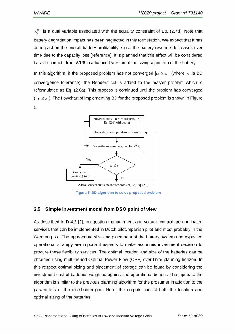
INVADE H2020 project – Grant nº 731148
D5.3- Placement and Sizing of Batteries in Low and Medium Voltage Grids Page 19 of 39
( )l
s is a dual variable associated with the equality constraint of Eq. (2.7d). Note that
battery degradation impact has been neglected in this formulation. We expect that it has
an impact on the overall battery profitability, since the battery revenue decreases over
time due to the capacity loss [reference]. It is planned that this effect will be considered
based on inputs from WP6 in advanced version of the sizing algorithm of the battery.
In this algorithm, if the proposed problem has not converged , (where is BD
convergence tolerance), the Benders cut is added to the master problem which is
reformulated as Eq. (2.6a). This process is continued until the problem has converged
( ). The flowchart of implementing BD for the proposed problem is shown in Figure
5.
Solve the initial master problem, i.e.,
Eq. (2.6) without (a)
Solve the master problem with cuts
Solve the sub-problem, i.e., Eq. (2.7)
Add a Benders cut to the master problem, i.e., Eq. (2.6)
No
Converged
solution (stop)
Yes
Figure 5. BD algorithm to solve proposed problem
2.5 Simple investment model from DSO point of view
As described in D 4.2 [2], congestion management and voltage control are dominated
services that can be implemented in Dutch pilot, Spanish pilot and most probably in the
German pilot. The appropriate size and placement of the battery system and expected
operational strategy are important aspects to make economic investment decision to
procure these flexibility services. The optimal location and size of the batteries can be
obtained using multi-period Optimal Power Flow (OPF) over finite planning horizon. In
this respect optimal sizing and placement of storage can be found by considering the
investment cost of batteries weighted against the operational benefit. The inputs to the
algorithm is similar to the previous planning algorithm for the prosumer in addition to the
parameters of the distribution grid. Here, the outputs consist both the location and
optimal sizing of the batteries.
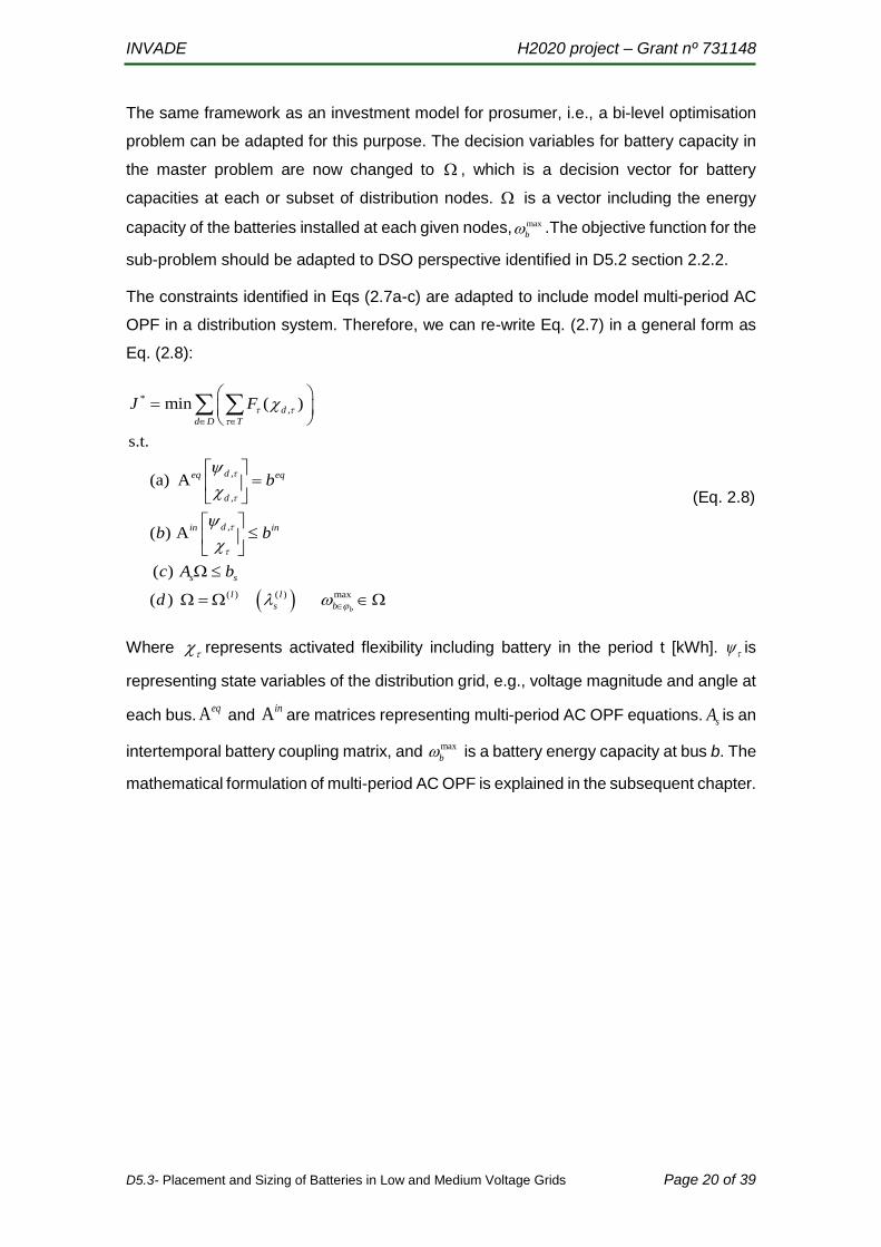
INVADE H2020 project – Grant nº 731148
D5.3- Placement and Sizing of Batteries in Low and Medium Voltage Grids Page 20 of 39
The same framework as an investment model for prosumer, i.e., a bi-level optimisation
problem can be adapted for this purpose. The decision variables for battery capacity in
the master problem are now changed to , which is a decision vector for battery
capacities at each or subset of distribution nodes. is a vector including the energy
capacity of the batteries installed at each given nodes, max
b .The objective function for the
sub-problem should be adapted to DSO perspective identified in D5.2 section 2.2.2.
The constraints identified in Eqs (2.7a-c) are adapted to include model multi-period AC
OPF in a distribution system. Therefore, we can re-write Eq. (2.7) in a general form as
Eq. (2.8):
*
,
,
,
,
( ) ( ) max
min ( )
s.t.
(a) A
( ) A
( )
( )
b
d
d D T
deq eq
d
din in
s s
l l
s b
J F
b
b b
c A b
d
(Eq. 2.8)
Where represents activated flexibility including battery in the period t [kWh]. is
representing state variables of the distribution grid, e.g., voltage magnitude and angle at
each bus. Aeq and A
inare matrices representing multi-period AC OPF equations. sA is an
intertemporal battery coupling matrix, and max
b is a battery energy capacity at bus b. The
mathematical formulation of multi-period AC OPF is explained in the subsequent chapter.

INVADE H2020 project – Grant nº 731148
D5.3- Placement and Sizing of Batteries in Low and Medium Voltage Grids Page 21 of 39
2.5.1 Representation of multi-period AC optimal power flows constraints
NOMENCLATURE
1) Indices and Sets:
(b,j), t,l, k Indices of bus, time, linearization segments of voltage magnitude term and circular
constraint
b, t, l, k Sets of bus, time, linearization segments of voltage magnitude term and circular
constraint
2) Parameters:
A Bus incidence matrix (if line existed between buses b and j, Ab,j is equal to
1,otherwise zero)
g, b, y Line conductance, susceptance, admittance in pu
PG, QG Active and reactive power generation in pu
PD, QD Active and reactive load in pu
max,b jSL Maximum loading of distribution line
T Operating horizon, i.e., 6 hours, 12 hours, 24 hours or 48 hours
Vmax, Vmin, Vref Maximum and minimum voltage and voltage magnitude for reference bus in pu
Y The network admittance matrix in pu
max min, Maximum and minimum boundary of batteries state of charge in pu
,ch disη η Efficiency parameter for charging and discharging battery, respectively
3) Variables: All variables are in per unit (pu)
ID, IE, IG, IL Load, parking lot, station and line current
PL, QL line active and reactive power, respectively
V, V, Magnitude, deviation and angle of voltage
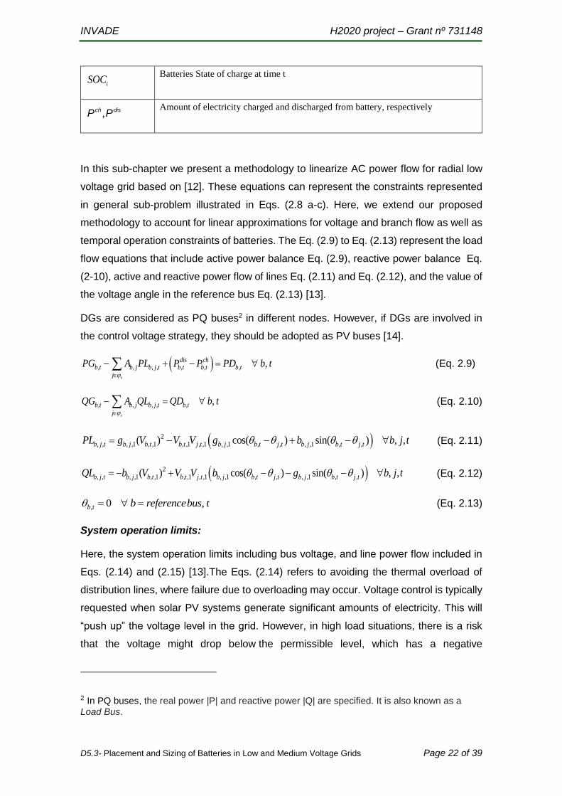
INVADE H2020 project – Grant nº 731148
D5.3- Placement and Sizing of Batteries in Low and Medium Voltage Grids Page 22 of 39
tSOC
Batteries State of charge at time t
,ch disP P Amount of electricity charged and discharged from battery, respectively
In this sub-chapter we present a methodology to linearize AC power flow for radial low
voltage grid based on [12]. These equations can represent the constraints represented
in general sub-problem illustrated in Eqs. (2.8 a-c). Here, we extend our proposed
methodology to account for linear approximations for voltage and branch flow as well as
temporal operation constraints of batteries. The Eq. (2.9) to Eq. (2.13) represent the load
flow equations that include active power balance Eq. (2.9), reactive power balance Eq.
(2-10), active and reactive power flow of lines Eq. (2.11) and Eq. (2.12), and the value of
the voltage angle in the reference bus Eq. (2.13) [13].
DGs are considered as PQ buses2 in different nodes. However, if DGs are involved in
the control voltage strategy, they should be adopted as PV buses [14].
, , , , , , , ,
b
dis chb t b j b j t b t b t b t
j
PG A PL P P PD b t
(Eq. 2.9)
, , , , , ,
b
b t b j b j t b t
j
QG A QL QD b t
(Eq. 2.10)
2, , , ,1 , ,1 , ,1 , ,1 , ,1 , , , ,1 , ,( ) cos( ) sin( ) , ,b j t b j b t b t j t b j b t j t b j b t j tPL g V V V g b b j t (Eq. 2.11)
2, , , ,1 , ,1 , ,1 , ,1 , ,1 , , , ,1 , ,( ) cos( ) sin( ) , ,b j t b j b t b t j t b j b t j t b j b t j tQL b V V V b g b j t (Eq. 2.12)
, 0 ,b t b referencebus t (Eq. 2.13)
System operation limits:
Here, the system operation limits including bus voltage, and line power flow included in
Eqs. (2.14) and (2.15) [13].The Eqs. (2.14) refers to avoiding the thermal overload of
distribution lines, where failure due to overloading may occur. Voltage control is typically
requested when solar PV systems generate significant amounts of electricity. This will
“push up” the voltage level in the grid. However, in high load situations, there is a risk
that the voltage might drop below the permissible level, which has a negative
2 In PQ buses, the real power |P| and reactive power |Q| are specified. It is also known as a Load Bus.

INVADE H2020 project – Grant nº 731148
D5.3- Placement and Sizing of Batteries in Low and Medium Voltage Grids Page 23 of 39
consequence on safeguard of operating the system; therefore, Eq. (2.15) ensures that
the voltage levels are maintained within the voltage permissible limits.
2 2 max 2, , , , ,( ) ( ) ( ) , ,b j t b j t b jPL QL SL b j t (Eq. 2.14)
min max, ,1 ,b tV V V b t (Eq. 2.15)
Temporal operation constraints of operating batteries:
The temporal constraints of operating batteries are presented in Eqs. (2.17) to (2.19).
The temporal problem implies a coupling of multiple time steps to ensure coherence of
the battery SOC between each consecutive time step. The spatial problem implies the
consideration of all nodes as possible placement locations for storage devices.
As we have already discussed that, the operating time horizon can range from 6 hours
to two days. The time steps of T are then coupled in order to successfully complete an
annual analysis.
, , 1 , ,
1 ch dis
b t b t b t dis b t
ch
SOC SOC P η Pη
(Eq. 2.16)
ch max
,0 ch
b t bP P (Eq. 2.17)
dis max
,0 dis
b t bP P (Eq. 2-18)
min max
,
b b t bSOC (Eq. 2.19)
,0 ,Tb bSOC SOC (Eq.
2.20)
The battery state of charge, i.e. the storage content, for battery unit in period t depends
on the state of charge in the previous period, and charging or discharging in current
period. These impacts are replicated by Eq. (2.16). The charging and discharging and
the SOC must be within minimum and maximum limits as expressed in Eqs. (2.17) to
Eq. (2.19). An additional constraint is added to avoid daily (if T is 24 hours) accumulation
effects by forcing the SOC of the first and last time step of the operating time horizon be
equal as stated in equation (2-20).
The proposed problem is a nonlinear programming (NLP) model due to non-linear Eq.
(2.11), Eq. (2.12), and circular inequality of Constraint (2.15). Moreover, NLP problems
are intrinsically more difficult to solve compared to linear problems, and there is no
guarantee to reach optimal solution [13]. Hence, we need to develop a linearized OPF
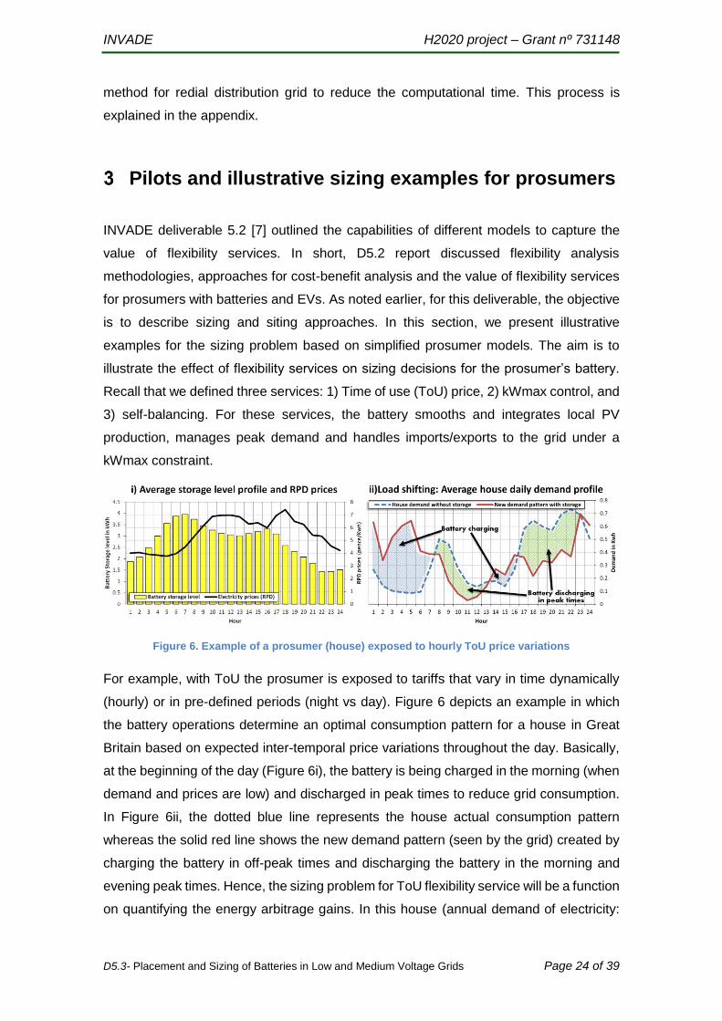
INVADE H2020 project – Grant nº 731148
D5.3- Placement and Sizing of Batteries in Low and Medium Voltage Grids Page 24 of 39
method for redial distribution grid to reduce the computational time. This process is
explained in the appendix.
Pilots and illustrative sizing examples for prosumers
INVADE deliverable 5.2 [7] outlined the capabilities of different models to capture the
value of flexibility services. In short, D5.2 report discussed flexibility analysis
methodologies, approaches for cost-benefit analysis and the value of flexibility services
for prosumers with batteries and EVs. As noted earlier, for this deliverable, the objective
is to describe sizing and siting approaches. In this section, we present illustrative
examples for the sizing problem based on simplified prosumer models. The aim is to
illustrate the effect of flexibility services on sizing decisions for the prosumer’s battery.
Recall that we defined three services: 1) Time of use (ToU) price, 2) kWmax control, and
3) self-balancing. For these services, the battery smooths and integrates local PV
production, manages peak demand and handles imports/exports to the grid under a
kWmax constraint.
Figure 6. Example of a prosumer (house) exposed to hourly ToU price variations
For example, with ToU the prosumer is exposed to tariffs that vary in time dynamically
(hourly) or in pre-defined periods (night vs day). Figure 6 depicts an example in which
the battery operations determine an optimal consumption pattern for a house in Great
Britain based on expected inter-temporal price variations throughout the day. Basically,
at the beginning of the day (Figure 6i), the battery is being charged in the morning (when
demand and prices are low) and discharged in peak times to reduce grid consumption.
In Figure 6ii, the dotted blue line represents the house actual consumption pattern
whereas the solid red line shows the new demand pattern (seen by the grid) created by
charging the battery in off-peak times and discharging the battery in the morning and
evening peak times. Hence, the sizing problem for ToU flexibility service will be a function
on quantifying the energy arbitrage gains. In this house (annual demand of electricity:

INVADE H2020 project – Grant nº 731148
D5.3- Placement and Sizing of Batteries in Low and Medium Voltage Grids Page 25 of 39
3.8 MWh, no PV considered), three battery sizes were tested: 1.4kWh, 2.9kWh, and
4.3kWh which produced cost savings (reduction to the annual electricity bill) in the
magnitude of 7%, 11% and 15% compared to not having the battery in the house.
However, if other flexibility services are included for battery operations the value will
increase and hence affect the battery size. In this chapter, we look at the kWmax service
and self-balancing services impact on the prosumers PV-battery sizing decisions.
3.1 Flexibility needed due to kWmax and self-balancing
In the next sections, we discuss the prosumer sizing problem by considering the effects
of flexibility services for kWmax control and self-balancing. On one hand, kWmax
constraints RES exports (also grid imports) and therefore might limit installation of
additional RES capacity for the prosumer. In this case, the battery provides the flexibility
to manage kWmax limitations, which allows installing more solar capacity. On the other
hand, flexibility for self-balancing maximizes RES utilization by better matching supply-
demand operations. In short, given the limitations of kWmax, how much PV is installable
based on the size of the battery? If we increase on-site solar capacity, what battery size
will be required to support this deployment? These questions are discussed by simulating
the installation of a battery in two INVADE pilots (following section). This preliminary
analysis employs available simplified operational models previously developed by
NTNU. The scope of the analysis is to show battery-solar size combinations for the
prosumer and estimate the operational value of the battery. For this purpose, a sensitivity
analysis on different sizes for batteries and PV is performed as follows:
1. Show PV installation subjected to a kWmax
First case: No storage considered or present in the prosumer system
2. Battery supports solar PV deployment (increase capacity)
1. Battery presence increases RES capacity
2. Through the simplified operational model illustrate the operational value
of having a battery showing the benefits
3. Different storage capacities tested (sizing problem) along with increased solar PV
capacity

INVADE H2020 project – Grant nº 731148
D5.3- Placement and Sizing of Batteries in Low and Medium Voltage Grids Page 26 of 39
3.2 INVADE pilots data collection for simplified model
To implement the simplified operational models in the INVADE pilots, we attempted to
collect data from the different partners involved in the INVADE project. At the moment,
most of the pilots are being set up and consequently data is not yet available. However,
we were able to gather some applicable information from the house pilots in the
Netherlands and from the Albena hotel in Bulgaria. Based on this limited data, we
illustrate and discuss the sizing problem for different battery and solar PV sizes. The
details regarding data collection, assumptions and model implementation are explained
in the next subsections.
3.2.1 INVADE pilot: Homes in the Netherlands
The pilot in Netherlands is split in several categories with the main goal to include as
much as renewable energy possible by using on-site batteries and electrical vehicles.
The pilot is divided in: 1) Small scale homes with smart charging, 2) large scale offices
and parking lots containing several charge points for EVs, and 3) a large public case with
thousands charge points. From these three cases, small scale homes have been chosen
to illustrate the sensibility of battery sizes on PV integration and kWmax control. This is
due to the availability of data provided by Elaad (Dutch INVADE partner) as well as to
show the sizing problem for small prosumers (houses) while the Bulgarian case (Albena,
following section) shows the case of large prosumer (a hotel). Hence, in this way, we can
present and discuss two different prosumer perspectives.
3.2.1.1 Data sets used, assumptions and limitations
For the small scale home simulation of Arnhem, Elaad recommended to this deliverable
the usage of some basic data sources. For example, home load data were taken from a
standardized profile for Dutch houses. Actual demand data from the home pilot is not yet
available or cannot be shared due to privacy limitations. In summary, the following data
sets were collected:
- Load data was obtained from the Dutch organization NEDU3. It provides standard
consumption profiles of small consumers. These profiles are used by grid
operators to estimate the allocation of energy to small consumers on a daily
basis. Therefore, a profile is typically used to estimate for a certain period what
3 http://www.nedu.nl/portfolio/verbruiksprofielen/

INVADE H2020 project – Grant nº 731148
D5.3- Placement and Sizing of Batteries in Low and Medium Voltage Grids Page 27 of 39
the consumption will be. There are ten profiles for electricity. The dataset consists
of 15 min demand time-steps spread over a year that together contain the entire
annual consumption. The sum of all profile fractions is one. In order to represent
a typical Dutch house, the sum of the profile fractions is multiplied by the annual
consumption. For our illustrative sizing example, we have used two profiles: 1)
the “E3A” profile in which we assume a 3.5MWh annual consumption and 2) the
E1C profile in which we assume a 4MW annual consumption under ToU price
regime throughout the day (7am to 9pm).
- Solar potentials: Temperature and irradiation data were downloaded from the
national weather service station closest to Arnhem. Then, this dataset was
converted to PV production. We used the methodology conversion noted in [15]
.
- Electricity prices: spot market electricity price was taken from the APEX website
and other sources. Also NEDU publishes typical electricity prices for households
under different profiles. The electricity price is asset under a fix retail price of 41
€/MWh.
3.2.1.2 Model description
The simplified operational model implemented for the Dutch houses was based on the
multi-period optimization model initially developed and implemented in Crespo del
Granado et. al (2014) [15]. It is a model with emphasis on electricity storage presence in
houses. The model minimizes the marginal cost of supplying energy to the house in
hourly basis within the day. Wholesale spot price or day ahead market electricity prices
are used as inputs for the cost of electricity (i.e. BRP application). The model objective
is to minimize the total energy grid consumption cost over a finite horizon (one day
discretized in hourly or finer time steps) by employing electricity storage for peak shaving
and smoothing renewable generation. Therefore, the model optimizes battery operations
to: 1) charge when energy spot prices are low and discharge when prices are high, and
2) saving local solar surplus. In a nutshell, the house model contains the following
features: the objective function (minimizes grid consumption), a supply demand balance
equation, and the storage inter-temporality equilibrium constraint along with the limits on
the battery charging/discharging flow rates and capacity.
3.2.2 INVADE pilot: Hotel in Albena, Bulgaria
The five-star-hotel Flamingo Grand is an end-user with a high energy consumption,
resulting in high savings potential by installation of a smart energy system. Their demand

INVADE H2020 project – Grant nº 731148
D5.3- Placement and Sizing of Batteries in Low and Medium Voltage Grids Page 28 of 39
profile is ideal for a PV installation due to high consumption during daytime [16]. In
addition, grid utility tariffs are calculated from the monthly peak load, making high peak
loads very costly for the hotel. Thus, self-balancing through installation of a battery could
reduce these peaks. The load profile of the hotel is season dependent, where the
summer is the most power intensive period due to a high number of guests. However, if
a high PV production day occurs in a day with a low amount of guests, the net load could
turn negative. According to D10.1 [16], prosumers are not compensated economically
for injecting power into the grid. On the contrary, it could potentially become a problem
as Bulgarian DSOs are not used to prosumers. Therefore, the battery is also important
in order to avoid a negative net load where power is injected into the grid.
Season use:
1. Summer – In the summer there is high PV production and high demand due to
many guests. High PV production will take care of the high peak loads in the
middle of the day, but the potential high evening load described in D10.1 [16]
can be partially covered by the battery.
2. Autumn / Spring – Although hotel activity is reduced in the autumn and spring,
high PV production could still occur. In the instance of high PV production and
low consumption, the battery can be used for self-balancing to avoid injecting
power into the grid.
3. Winter – Both energy consumption and PV production is low, and the battery
can be operated freely in order to reduce own costs. In low activity periods, self-
balancing is not as necessary as in the high season. During these periods, there
is greater potential for the battery to work as a flexible resource on the day-
ahead and intraday market for a FO or BRP. Note that FO/BRP perspective is
not included in phase 1, and therefore not described further.
3.2.3 Data sets used, assumptions and limitations
The data used to run simulations for the hotel are load, temperature, irradiation and
energy price data. In the results presented in this deliverable, load data from July to
September 2017 provided by Albena was used. However, the PV data, which were
provided, were from January to July 2017, which makes it hard to create correct results
because the data don’t correlate. Therefore, an open source satellite based service was
used to find PV data for the relevant months. However, the data used is then from 2014,
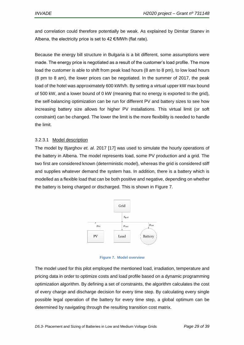
INVADE H2020 project – Grant nº 731148
D5.3- Placement and Sizing of Batteries in Low and Medium Voltage Grids Page 29 of 39
and correlation could therefore potentially be weak. As explained by Dimitar Stanev in
Albena, the electricity price is set to 42 €/MWh (flat rate).
Because the energy bill structure in Bulgaria is a bit different, some assumptions were
made. The energy price is negotiated as a result of the customer’s load profile. The more
load the customer is able to shift from peak load hours (8 am to 8 pm), to low load hours
(8 pm to 8 am), the lower prices can be negotiated. In the summer of 2017, the peak
load of the hotel was approximately 600 kWh/h. By setting a virtual upper kW max bound
of 500 kW, and a lower bound of 0 kW (meaning that no energy is exported to the grid),
the self-balancing optimization can be run for different PV and battery sizes to see how
increasing battery size allows for higher PV installations. This virtual limit (or soft
constraint) can be changed. The lower the limit is the more flexibility is needed to handle
the limit.
3.2.3.1 Model description
The model by Bjarghov et. al. 2017 [17] was used to simulate the hourly operations of
the battery in Albena. The model represents load, some PV production and a grid. The
two first are considered known (deterministic model), whereas the grid is considered stiff
and supplies whatever demand the system has. In addition, there is a battery which is
modelled as a flexible load that can be both positive and negative, depending on whether
the battery is being charged or discharged. This is shown in Figure 7.
Figure 7. Model overview
The model used for this pilot employed the mentioned load, irradiation, temperature and
pricing data in order to optimize costs and load profile based on a dynamic programming
optimization algorithm. By defining a set of constraints, the algorithm calculates the cost
of every charge and discharge decision for every time step. By calculating every single
possible legal operation of the battery for every time step, a global optimum can be
determined by navigating through the resulting transition cost matrix.

INVADE H2020 project – Grant nº 731148
D5.3- Placement and Sizing of Batteries in Low and Medium Voltage Grids Page 30 of 39
3.3 Implementation and illustrative preliminary results
3.3.1 Battery-PV sizing for houses in Netherlands
The simulations for the small houses in Netherlands are in one-hour resolution. The data
collected allowed simulating one year. The model horizon performs this simulation for
each day separately. Hence, the model is run 365 times as it assumes that is rather
unrealistic to have perfect knowledge on solar-load patterns beyond 24hours (for a
discussion on planning horizon, see chapter 4 in D5.3 “Flexibility operations algorithms”).
Figure 8 depicts typical results on simulating supply-demand operations and taking into
account the decisions for battery charge/discharge levels. In Figure 8a, observe that the
battery at the begging of the day (dotted red-lines) has a low energy content. The
reasoning is to have at is lowest in order to be ready for the solar surplus happening at
the middle of the day (Figure 8b and Figure 8c). In this period, the battery tries to charge
as much as possible, but this is still not enough for self-balancing and the surplus is
exported to the grid. For this particular example, we arbitrarily set a kWmax limit of 1kWh.
Throughout the year, demand exceeds this limit only in 6 days and hence the battery use
for this flexibility service was not significant. However, for larger PV sizes, the solar
surplus (exports) exceed 1kWh more frequently.
Figure 8. Three-day (in summer) example of supply-demand dynamics in the house
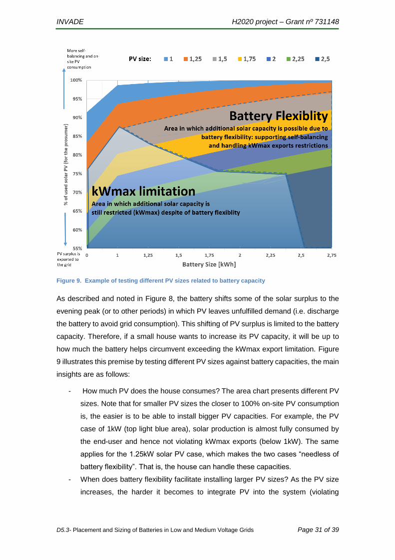
INVADE H2020 project – Grant nº 731148
D5.3- Placement and Sizing of Batteries in Low and Medium Voltage Grids Page 31 of 39
Figure 9. Example of testing different PV sizes related to battery capacity
As described and noted in Figure 8, the battery shifts some of the solar surplus to the
evening peak (or to other periods) in which PV leaves unfulfilled demand (i.e. discharge
the battery to avoid grid consumption). This shifting of PV surplus is limited to the battery
capacity. Therefore, if a small house wants to increase its PV capacity, it will be up to
how much the battery helps circumvent exceeding the kWmax export limitation. Figure
9 illustrates this premise by testing different PV sizes against battery capacities, the main
insights are as follows:
- How much PV does the house consumes? The area chart presents different PV
sizes. Note that for smaller PV sizes the closer to 100% on-site PV consumption
is, the easier is to be able to install bigger PV capacities. For example, the PV
case of 1kW (top light blue area), solar production is almost fully consumed by
the end-user and hence not violating kWmax exports (below 1kW). The same
applies for the 1.25kW solar PV case, which makes the two cases “needless of
battery flexibility”. That is, the house can handle these capacities.
- When does battery flexibility facilitate installing larger PV sizes? As the PV size
increases, the harder it becomes to integrate PV into the system (violating

INVADE H2020 project – Grant nº 731148
D5.3- Placement and Sizing of Batteries in Low and Medium Voltage Grids Page 32 of 39
kWmax). This is illustrated in the chart area “Battery Flexibility”. Consider the 1.5
PV size (grey area), here the solar production is exceeding the pretended 1kW
control limit, hence PV this size could not be installed in the house. This is the
case when there is no battery presence (kWh=0). However, once the battery size
is 1kW, there is enough flexibility in the system and hence the solar PV can be
increased. Similar trend occurs for larger PV sizes based on the increase of
battery size.
- How kWmax and self-balancing limit greater PV capacities? Under the kWmax
limitation area in the chart, we observe that for larger PV capacities (>1.5), it
becomes increasingly difficult to self-balance PV. Despite of having a battery, the
PV surplys overcomes the possible flexibility provided by the battery. For
instance, a 1kWh battery along with a 1.75kWh solar PV will be charged in couple
of time steps and hence the solar surplus will start exceeding the kWmax
limitations. Therefore, this PV size is not suitable for installation in the house.
However, as the battery size increases, observe that the possibilities to increase
PV capacity improves.
Based on Figure 9, we calculate the savings on installing the possible PV-battery combo
sizes. That is, the value of having a battery compared to not having the battery installed.
This is calculated as savings (in %) on the energy bill. Figure 10 shows these results in
which the values with greater PV size produce the larger savings. The size of the battery
plays a major role since, as more PV surplus will occur, the more the battery will support
self-balancing the additional PV capacity. Hence, the higher the savings.

INVADE H2020 project – Grant nº 731148
D5.3- Placement and Sizing of Batteries in Low and Medium Voltage Grids Page 33 of 39
Figure 10. Cost savings for different Batter-PV six combinations
3.3.2 Battery-PV sizing for Albena
As we know that the energy tariff in Bulgaria is flat and by moving the demand from peak
hour to off-peak hours, a new lower flat energy tariff can be negotiated with the
retailer. The value of flexibility is calculated by simulation with the load data available
from 08th June 2017 till 18th September 2017. The hotel base load is 344 kWh/h on
average and peaks at 595 kWh/h. It is to be noted that this period of the year has
maximum demand compared to the rest of the periods of the year. For the given load
data, to respect the 500 kW grid import limit a 250 kWh battery is needed without any
local PV generation. The minimum PV generation capacity required to minimize the
investment cost of battery is 100 kW and the corresponding battery capacity is 75 kWh.
Further addition of battery capacity will not add any value to the flexibility as shown in
the figure. The value of this additional flexibility can be calculated only if the relation
between the normal and reduced tariff are known. As there is a strong correlation
between the PV generation and the demand, the electricity bill can be further reduced
by adding more PV generation capacity. The maximum PV capacity the 75 kWh battery
can handle is 425 kWp. Further addition of PV is possible with additional battery capacity.
Otherwise, part of the PV production has to be curtailed in real time to avoid the energy
export to the grid, as the grid code in Bulgaria might not support (and certainly does not
promote) RES injection from the consumers. The battery capacity required to support
500 kWp PV installation is 250 kWh without curtailment of PV generation. Figure 11
shows the associated energy cost for the grid import for every installed capacity of PV
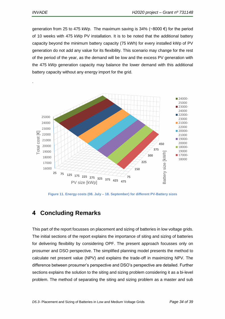
INVADE H2020 project – Grant nº 731148
D5.3- Placement and Sizing of Batteries in Low and Medium Voltage Grids Page 34 of 39
generation from 25 to 475 kWp. The maximum saving is 34% (~8000 €) for the period
of 10 weeks with 475 kWp PV installation. It is to be noted that the additional battery
capacity beyond the minimum battery capacity (75 kWh) for every installed kWp of PV
generation do not add any value for its flexibility. This scenario may change for the rest
of the period of the year, as the demand will be low and the excess PV generation with
the 475 kWp generation capacity may balance the lower demand with this additional
battery capacity without any energy import for the grid.
.
Figure 11. Energy costs (08. July – 18. September) for different PV-Battery sizes
Concluding Remarks
This part of the report focusses on placement and sizing of batteries in low voltage grids.
The initial sections of the report explains the importance of siting and sizing of batteries
for delivering flexibility by considering OPF. The present approach focusses only on
prosumer and DSO perspective. The simplified planning model presents the method to
calculate net present value (NPV) and explains the trade-off in maximizing NPV. The
difference between prosumer’s perspective and DSO’s perspective are detailed. Further
sections explains the solution to the siting and sizing problem considering it as a bi-level
problem. The method of separating the siting and sizing problem as a master and sub
75
150
225
300
375
450
16000
17000
18000
19000
20000
21000
22000
23000
24000
25000
25 75 125 175 225 275 325 375 425 475 Ba
tte
ry s
ize
[kW
h]
To
tal co
st [€
]
PV size [kWp]
24000-2500023000-2400022000-2300021000-2200020000-2100019000-2000018000-1900017000-18000
INVADE H2020 project – Grant nº 731148
D5.3- Placement and Sizing of Batteries in Low and Medium Voltage Grids Page 35 of 39
problem, the iterative approach by adding benders cut to the master problem to achieve
optimal solution are detailed in the next section. Next section details the problem in DSO
perspective, the nonlinearity associated with the OPF problem and the method of mixed
linear programing approach to solve the problem with piece-vise linearization. Further
section describes investment analyses for storage and RES with illustrative examples
showing analysis for two pilot sites at Bulgaria and The Netherlands. The Bulgarian
example shows the battery sizing, PV sizing and the savings related to energy import
from the grid for different combination of batteries and PVs for a large prosumer. The
Netherlands example shows similar calculations for small homes.
The focus of the next deliverable D5.4 will be on extended operational model with an
elaborate battery and flexible load models to deliver flexibility services.
References
[1]. Lloret, P. and P. Olivella, INVADE architecture of pilots, D4.2, 2017, INVADE project.
[2]. Capitanescu, F., Critical review of recent advances and further developments needed in AC optimal power flow. Electric Power Systems Research, 2016. 136(Supplement C): p. 57-68.
[3]. Baker, K., G. Hug, and X. Li, Energy Storage Sizing Taking Into Account Forecast Uncertainties and Receding Horizon Operation. IEEE Transactions on Sustainable Energy, 2017. 8(1): p. 331-340.
[4]. Ghofrani, M., et al., A Framework for Optimal Placement of Energy Storage Units Within a Power System With High Wind Penetration. IEEE Transactions on Sustainable Energy, 2013. 4(2): p. 434-442.
[5]. Atwa, Y.M. and E.F. El-Saadany, Optimal Allocation of ESS in Distribution Systems With a High Penetration of Wind Energy. IEEE Transactions on Power Systems, 2010. 25(4): p. 1815-1822.
[6]. Grover-Silva, E., R. Girard, and G. Kariniotakis, Optimal sizing and placement of distribution grid connected battery systems through an SOCP optimal power flow algorithm. Applied Energy, 2017.
[7]. Korpås, M., et al., Methods for assessing the value of flexibility in distribution grids, in D 5.2. 2017: INVADE project.
[8]. Colson, B., P. Marcotte, and G. Savard, An overview of bilevel optimization. Annals of Operations Research, 2007. 153(1): p. 235-256.
[9]. Benders, J.F., Partitioning procedures for solving mixed-variables programming problems. Numer. Math., 1962. 4(1): p. 238-252.
[10]. Fortenbacher, P., A. Ulbig, and G. Andersson, Optimal Placement and Sizing of Distributed Battery Storage in Low Voltage Grids using Receding Horizon Control Strategies. IEEE Transactions on Power Systems, 2017: p. 1-1.
INVADE H2020 project – Grant nº 731148
D5.3- Placement and Sizing of Batteries in Low and Medium Voltage Grids Page 36 of 39
[11]. Fortenbacher, P., On the Integration of Distributed Battery Storage in Low Voltage Grids. 2017, ETH Zurich.
[12]. Pirouzi, S., et al. Proactive Operation of Electric Vehicles in Harmonic Polluted Smart Distribution Networks. IET Generation, Transmission & Distribution, 2017.
[13]. Pirouzi, S., et al., Robust linear architecture for active/reactive power scheduling of EV integrated smart distribution networks. Electric Power Systems Research, 2018. 155(Supplement C): p. 8-20.
[14]. Gallego, L.A., E. Carreno, and A. Padilha-Feltrin. Distributed generation modelling for unbalanced three-phase power flow calculations in smart grids. in 2010 IEEE/PES Transmission and Distribution Conference and Exposition: Latin America (T&D-LA). 2010.
[15]. Crespo Del Granado, P., S.W. Wallace, and Z. Pang, The value of electricity storage in domestic homes: a smart grid perspective. Energy Systems, 2014. 5(2): p. 211-232.
[16]. Cordobés, C., Pilot Specifications, D 10.1, 2017, INVADE project.
[17]. Sigurd Nikolai Bjarghov, Utilizing EV Batteries as a Flexible Resource at End-user Level, in Electric Power Engineering. 2017, Norwegian University of Science and Technology (NTNU): Master Thesis.
[18]. Wood, A. and B. Wollenberg, Power Generation, Operation, and Control. Wiley-Interscience.
[19]. Biswas, S., S.K. Goswami, and A. Chatterjee, Optimal distributed generation placement in shunt capacitor compensated distribution systems considering voltage sag and harmonics distortions. IET Generation, Transmission & Distribution, 2014. 8(5): p. 783-797.
[20]. Kavousi-Fard, A. and T. Niknam, Optimal Distribution Feeder Reconfiguration for Reliability Improvement Considering Uncertainty. IEEE Transactions on Power Delivery, 2014. 29(3): p. 1344-1353.
[21]. Castillo, A., et al., A successive linear programming approach to solving the iv-acopf. IEEE Transactions on Power Systems, 2016. 31(4): p. 2752-2763.

INVADE H2020 project – Grant nº 731148
D5.3- Placement and Sizing of Batteries in Low and Medium Voltage Grids Page 37 of 39
Appendix I
The Mixed Integer Linear Programing (MILP) Model
1) Linear approximation of power balance equations: constraints (2.11) and (2.12) in
the model are non-linear equations. For linear approximation of these constraints, this
paper considers the following assumptions [13]:
The difference of voltage angle between two buses (across a line) is less than
0.105 radian.
The voltage magnitude at the fundamental frequency can be written as
min
l
l
l
V V
based on the piecewise linearization method in [18] and Figure 12,
wherein V << 1.
It is expressed that the difference of voltage angle across a line is less than 0.105 radian
based on power flow results of different distribution networks [19, 20] that is shown in
Table 1. Therefore, based on the first assumption, sin (b-j) and cos (b-j) are equal to
(b-j) and 1, respectively. In addition, based on the second assumption, V2 and VbVj are
respectively equal to:
2
2 min
l
l l
l
V V m V
(Eq. 2.21)
2
min min min, ,
l l
b j b l j l
l l
V V V V V V V
(Eq. 2.22)
Where, m is the line slope. It is noted that V2, V×(b-j) and (b-j)2 are negligible, and
these terms are considered to be zero in this paper. Therefore, the linear approximation
of Eqs. (2.11) and (2-12) are as follows:
Table 1. Maximum difference of voltage angle across a line
Network 33-Bus 69-Bus 123-Bus
Maximum value of (i-j) -0.004 -0.006 -0.009

INVADE H2020 project – Grant nº 731148
D5.3- Placement and Sizing of Batteries in Low and Medium Voltage Grids Page 38 of 39
Figure 12. The piecewise linearization method [18]
2
min min min, , , ,1 , ,1, , ,1, , ,1 , ,( ) , ,
l
b j t b j l b t l j t l b j b t j t
l
PL g m V V V V V b b j t
(Eq. 2.23)
2
min min min, , , ,1 , ,1, , ,1, , ,1 , ,( ) , ,
l
b j t b j l b t l j t l b j b t j t
l
QL b m V V V V V g b j t
(Eq. 2.24)
Linear approximation of voltage limits, i.e., constraint (2.14) is re-written as Eq. (2.25).
max, , , , b t lV V b t l (Eq. 2.25)
Where, V is positive variable based on Figure 12, and Vmax is equal to (Vmax-Vmin)/Nl,
where Nl is the number of linearization segments of the voltage magnitude term. The
constraints (2.15) is a circular inequality. Based on idea presented in Figure 13, the linear
approximation equations of these constraints are written as follows:
max, , , , ,cos( ) cos( ) , , , b j t b j t b jk PL k QL SL b j t k (Eq. 2.26)
max, ,cos( ) cos( ) , , b t b t bk PG k QG SG b t k (Eq. 2.27)
Based on the above equations, the circular constraint is approximated by a polygon.
Each edge of the polygon is a straight line and their equations are obtained from the
tangents to the circle at different points depicted in Figure 13 [21]. In other words, these
equations linearized based on the method presented in Figure 13, but it should be noted
that we need enough piece-wise linear sections, in order to avoid high error. Therefore,
ΔV
V2
V
Segment
l
Line slope:
ml
Vmin
(Vmin)2

INVADE H2020 project – Grant nº 731148
D5.3- Placement and Sizing of Batteries in Low and Medium Voltage Grids Page 39 of 39
the number of piece-wise linear sections with different angles from horizontal axis should
be increased to reduce the linearization error. Hence, the 360 degrees of circle perimeter
are divided into equal parts α. Then, the line equation is linearized for each kα, where
k is the linearization segments index. Finally, the calculated line equation is integrated
into a circle with a radius less than or equal to S.
Figure 13. Linearization of circular constraint