smart city cluster collaboration, task 4. measurement and verification methodology for energy,...

1

Smart City Cluster Collaboration

Task 4 Data Centre Integration

Energy, Environmental, and Economic Efficiency Metrics: Measurement and Verification Methodology

2

Revision History

VERSION DATE PARTNERS DESCRIPTION/COMMENTS

4.1.1 2015 – 04 – 20 Jacinta Townley (GENiC /UTRCI)

Complied the work completed for Task 4.1

4.1.2 2015 – 04 – 22 Jaume Salom (RenewIT / IREC)

Comments

4.1.3 4.1.4 4.1.5

2015 – 04 – 28 2015 – 06 – 12 2015 – 06 – 12

Vasiliki Georgiadou (GEYSER / Green IT Amsterdam) Jacinta Townley (GENiC/UTRCI) Jacinta Townley (GENiC/UTRCI)

Review comments Updated sections based on comments, made some additional text change and added standardisation input. Updated ERE with footnote and extended intro section.

4.1.6 2015 – 06 - 25 Silvia Sanjoaquín Vives (DC4Cities/ GNF)

Last review


4.2.1 2015 – 04 – 24 Daniela Isidori (RenewIT/Loccioni)

Complied the work completed for Task 4.2

4.2.2 2015 – 05 – 18 Gonzalo Díaz Vélez / Silvia Sanjoaquín Vives (DC4Cities / GNF)

Document review


Document fixing after review

4.2.4 2015 – 06 – 01 Andrea Quintiliani (DC4Cities / ENEA)

Example for EES and few minor corrections in the EES chapter


Examples for all metrics except for GUF

4.2.6 2015 – 06 – 04 Daniela Isidori (RenewIT/Loccioni

Document fixing after review (Figures, Tables, Sections and Equations cross references)

4.2.7 2015 – 06 -04 Vasiliki Georgiadou (GEYSER / Green IT Amsterdam)

Review

4.2.8 2015 – 06 -18 Jaume Salom (RenewIT/Irec) Review 4.2.9 2015 – 06 -19 Daniela Isidori

(RenewIT/Loccioni) Last Review

4.2.10 2015-06-25 Silvia Sanjoaquín Vives (DC4Cities/ GNF)

Last review


4.1 2015 – 06 – 29 Alexis Aravanis (DOLFIN/Synelixis)

Task 4.1 and 4.2 consolidation

4.2 2015 -07 - 06 Silvia Sanjoaquín Vives (DC4Cities/GNF)

Last review

3

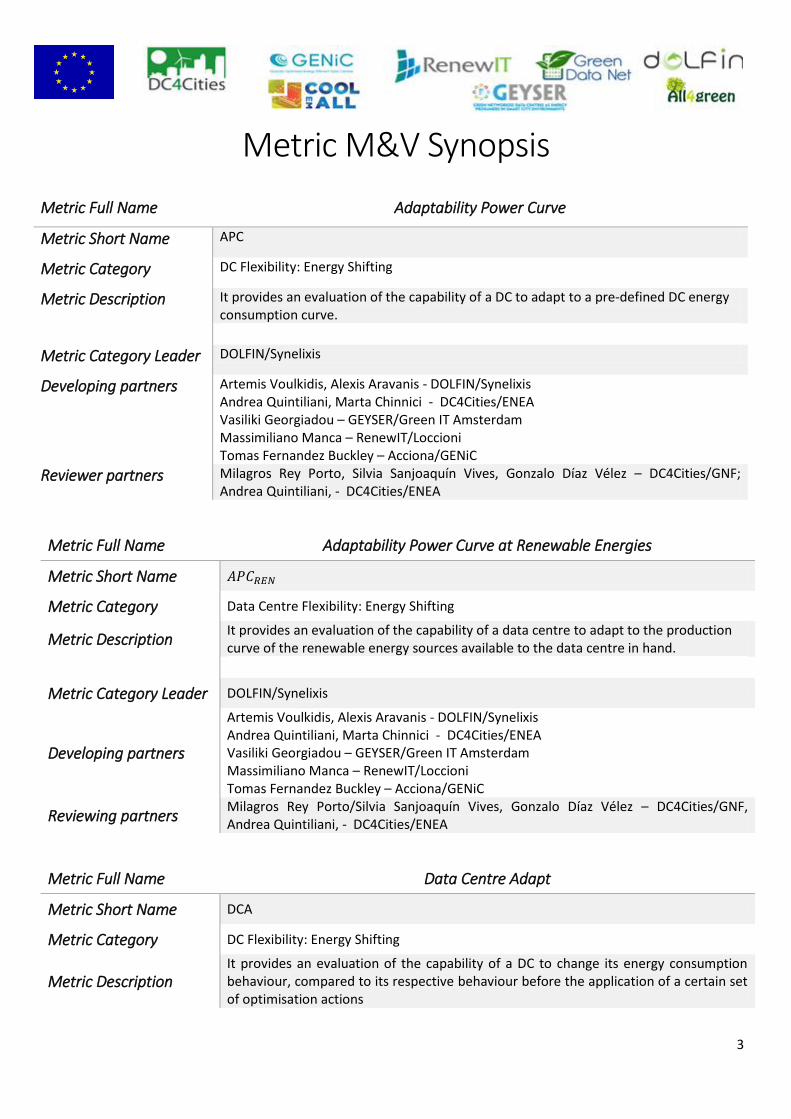
Metric M&V Synopsis

Metric Full Name Adaptability Power Curve

Metric Short Name APC

Metric Category DC Flexibility: Energy Shifting

Metric Description It provides an evaluation of the capability of a DC to adapt to a pre-defined DC energy consumption curve.

Metric Category Leader DOLFIN/Synelixis

Developing partners Artemis Voulkidis, Alexis Aravanis - DOLFIN/Synelixis Andrea Quintiliani, Marta Chinnici - DC4Cities/ENEA Vasiliki Georgiadou – GEYSER/Green IT Amsterdam Massimiliano Manca – RenewIT/Loccioni Tomas Fernandez Buckley – Acciona/GENiC

Reviewer partners Milagros Rey Porto, Silvia Sanjoaquín Vives, Gonzalo Díaz Vélez – DC4Cities/GNF; Andrea Quintiliani, - DC4Cities/ENEA

Metric Full Name Adaptability Power Curve at Renewable Energies

Metric Short Name

Metric Category Data Centre Flexibility: Energy Shifting

Metric Description It provides an evaluation of the capability of a data centre to adapt to the production curve of the renewable energy sources available to the data centre in hand.


Developing partners

Artemis Voulkidis, Alexis Aravanis - DOLFIN/Synelixis Andrea Quintiliani, Marta Chinnici - DC4Cities/ENEA Vasiliki Georgiadou – GEYSER/Green IT Amsterdam Massimiliano Manca – RenewIT/Loccioni Tomas Fernandez Buckley – Acciona/GENiC

Reviewing partners Milagros Rey Porto/Silvia Sanjoaquín Vives, Gonzalo Díaz Vélez – DC4Cities/GNF, Andrea Quintiliani, - DC4Cities/ENEA

Metric Full Name Data Centre Adapt

Metric Short Name DCA

Metric Category DC Flexibility: Energy Shifting

Metric Description It provides an evaluation of the capability of a DC to change its energy consumption behaviour, compared to its respective behaviour before the application of a certain set of optimisation actions

4


Developing partners

Artemis Voulkidis, Aravanis Alexis – DOLFIN/Synelixis Andrea Quintiliani, Marta Chinnici - DC4CITIES/ENEA Vasiliki Georgiadou – GEYSER/Green IT Amsterdam Massimiliano Manca – RenewIT/Loccioni Tomas Fernandez Buckley – Acciona/GENiC

Reviewing partners Milagros Rey Porto, Silvia Sanjoaquín Vives - GNF/DC4Cities, Andrea Quintiliani, - ENEA/DC4Cities

Metric Full Name Primary Energy Savings

Metric Short Name PE Savings

Metric Category PE Savings and CO2 avoided emissions

Metric Description The percentage of savings in terms of primary energy consumed by a data centre, once improvements have taken place with regard to its energetic, economic, or environmental management

Metric Category Leader Vasiliki Georgiadou (GEYSER / Green IT Amsterdam)

Developing partners Andrea Quintiliani, Marta Chinnici (DC4Cities / ENEA), Philip Inglesant (RenewIT / 451 Research), Davide Nardi Cesarini (RenewIT / Loccioni)

Reviewing partners Milagros Rey / Silvia Sanjoaquín Vives / Gonzalo Díaz Vélez (DC4Cities / GNF); Philip Inglesant (RenewIT/451 Research)

Metric Full Name CO2 Avoided Emissions

Metric Short Name CO2Savings

Metric Category PE Savings and CO2 avoided emissions

Metric Description The percentage of savings in terms of CO2 emissions generated by a data centre, once improvements have taken place with regard to its energetic, economic, or environmental management


Developing partners Andrea Quintiliani, Marta Chinnici (DC4Cities / ENEA), Philip Inglesant (RenewIT / 451 Research), Davide Nardi Cesarini (RenewIT / Loccioni)

Reviewing partners Milagros Rey Porto, Silvia Sanjoaquín Vives, Gonzalo Díaz Vélez (DC4Cities / GNF)

Metric Full Name Energy Expenses

Metric Short Name EES

Metric Category Economic savings in energy expenses

Metric Description A measure of how much the energy related expenses have changed in comparison to a baseline scenario, after having performed actions to upgrade the energetic, economic or environmental behaviour of a data centre

Metric Category Leader Andrea Quintiliani, Marta Chinnici (DC4Cities / ENEA)

5

Developing partners Vasiliki Georgiadou (GEYSER / Green IT Amsterdam)

Reviewing partners Milagros Rey Porto, Silvia Sanjoaquín Vives, Gonzalo Díaz Vélez (DC4Cities / GNF), Anthony Schoofs (GEYSER / Wattics)

Metric Full Name Grid Utilization Factor

Metric Short Name GUF

Metric Category Renewables integration: Energy produced locally and Renewable usage

Metric Description Percentage of time that the local generation does not cover the building demand, and thus how often energy must be supplied by the grid

Metric Category Leader Davide Nardi Cesarini (RenewIT/Loccioni), Jaume Salom (RenewIT/IREC)

Developing partners Artemis Voulkidis (Dolfin/Synelixis)

Reviewing partners Gonzalo Díaz Vélez / Silvia Sanjoaquín Vives, Gonzalo Díaz Vélez (DC4Cities / GNF)

Metric Full Name Energy Reuse Effectiveness

Metric Short Name ERE

Metric Category Energy Recovered: Heat Recovered

Metric Description Measures the benefit of reusing any recovered energy from the data centre


Developing partners Artemis Voulkidis, Alexis Aravanis (DOLFIN / Synelixis), Piotr Sobonski, Susan Rea, Christopher Burge (GENiC / CIT), Philip Inglesant (RenewIT / 451 Research)

Reviewing partners Fabrice Roudet ( GreenDataNet / Eaton), Milagros Rey Porto, Silvia Sanjoaquín Vives, Eduard Naranjo Cardoso (DC4Cities / GNF), Paul Hughes (GEYSER / ABB), Marco Cupelli (GEYSER / RWTH)

6

Contents 1 Introduction .............................................................................................................................................................. 8

2 Task 4.1 - Methodologies for existing Metrics .......................................................................................................... 9

2.1 Power Usage Effectiveness (PUE) ..................................................................................................................... 9

2.2 Renewable Energies Factor (REF) ................................................................................................................... 11

2.3 IT Equipment Energy Efficiency (ITEE) ............................................................................................................ 12

2.4 Cooling Effectiveness Rate (CER) .................................................................................................................... 12

2.5 Energy Reuse Effectiveness (ERE) ................................................................................................................... 14

2.5.1 M & V Plan Scope and Metric Overview ................................................................................................. 14

2.5.2 Measurements ........................................................................................................................................ 15

3 Task 4.2 – Methodologies for new Metrics............................................................................................................. 24

3.1 Adaptability Power Curve ............................................................................................................................... 24


3.1.2 Measurements ........................................................................................................................................ 25

3.1.3 Example ................................................................................................................................................... 28

3.2 Adaptability Power Curve at Renewable Energies .......................................................................................... 29


3.2.2 Measurements ........................................................................................................................................ 29

3.2.3 Example ................................................................................................................................................... 32

3.3 Data Centre Adapt .......................................................................................................................................... 33


3.3.2 Measurements ........................................................................................................................................ 34

3.3.3 Example ................................................................................................................................................... 37

3.4 Primary Energy Savings ................................................................................................................................... 38


3.4.2 Measurements ........................................................................................................................................ 39

3.4.3 Example ................................................................................................................................................... 44

3.5 CO2 Avoided Emissions.................................................................................................................................... 45


3.5.2 Measurements ........................................................................................................................................ 47

3.5.3 Example ................................................................................................................................................... 48

3.6 Economic Saving in Energy Expenses (EES) ..................................................................................................... 49


3.6.2 Measurements ........................................................................................................................................ 52

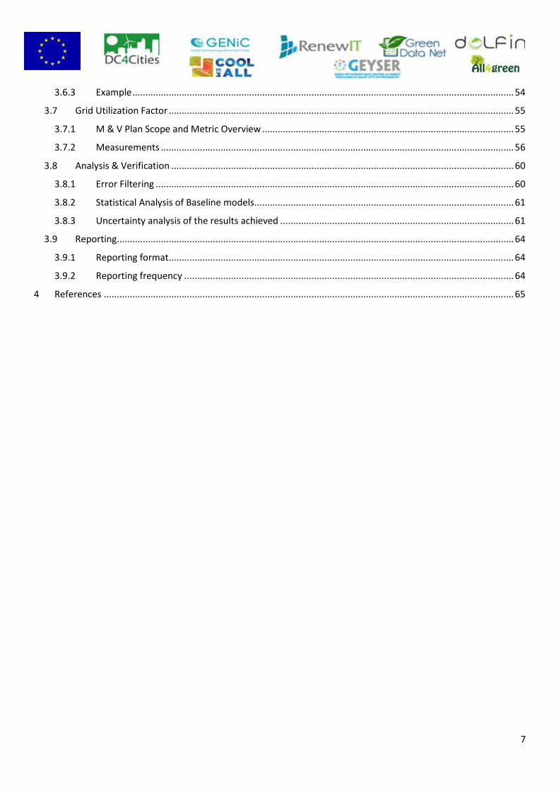
7

3.6.3 Example ................................................................................................................................................... 54

3.7 Grid Utilization Factor ..................................................................................................................................... 55


3.7.2 Measurements ........................................................................................................................................ 56

3.8 Analysis & Verification .................................................................................................................................... 60

3.8.1 Error Filtering .......................................................................................................................................... 60

3.8.2 Statistical Analysis of Baseline models .................................................................................................... 61

3.8.3 Uncertainty analysis of the results achieved .......................................................................................... 61

3.9 Reporting ......................................................................................................................................................... 64

3.9.1 Reporting format ..................................................................................................................................... 64

3.9.2 Reporting frequency ............................................................................................................................... 64

4 References .............................................................................................................................................................. 65

8

1 Introduction

The standardization activities performed so far in the context of the Smart City Cluster collaboration have led to the

identification of appropriate methodologies and procedures for the calculation of new and existing metrics or Key

Performance Indicators (KPIs). Thus, allowing the standardization of procedures to the extent possible and the

determination of common baselines for the efficient comparison of Cluster projects and the aggregation and

comparison of common variables and metrics, conflating seamlessly input from all Cluster constituent projects.

The projects included in the cluster, as already detailed in section 1 of Task 3 are the following: All4Green,

CoolEmAll, GreenDataNet, RenewIT, GENiC, GEYSER, Dolfin and DC4Cities. Moreover, since April 2015 a new project

has joined the cluster, EURECA. Every one of the above projects focuses on different goals and objectives,

quantifying the performance of the involved systems by measuring different events. Hence, the comparison of the

obtained measurements requires the definition of common variables and metrics to compare results in the same

way.

In this course, Task 3 proposed new metrics based on the existing ones improving their performance. In particular,

Task 3.1 identified existing metrics that could be employed in the context of Cluster, whereas Task 3.2 built upon the

current metrics to define new for measuring concepts as e.g. the exploitation of RES and the flexibility of DCs to

adjust their energy consumption and Task 3.3 defined new metrics for measuring the performance of DCs.

However, in the direction of defining common methodologies for the measurement of common KPIs toward a

collective standard development, Task 4 focused on the definition of common measuring and verification

methodologies. Specifically, Task 4.1 presented measuring and verification methodologies for existing metrics which

are almost finalized by standardization bodies (e.g. ISO/IEC JTC 1/SC 39), using the quasi-finalized metrics as

common basis for comparison. In addition, Task 4.2 presented measuring and verification methodologies for new

metrics defined in Cluster activity Task 3.2.

The measuring and verification methodologies defined in Task 4 are compliant with the International Performance

Measurement and Verification Protocol (IPMVP). The IPMVP is a protocol developed by a consortium of

international organizations, defining standards for energy efficiency projects. Capitalizing on the success of IPMVP,

Task 4 determines measuring and verification methodologies fully in line with the successful and pervasive

methodologies of IPMVP, giving rise to a coherent Cluster protocol, allowing for the efficient comparison of Cluster

projects and the exploitation of registered measurements toward amalgamation of feedback and the emergence of a

holistic approach allowing the drawing of common Cluster conclusions.

However, a fully developed strategy on how to deal with the data gathered, stored, and analysed for the purpose of

computing, reporting, and potentially auditing the related metrics is out of scope of this cluster's goals and activities.

As such, each case would need to be handled on an ad-hoc basis, depending also on the data management systems

already in place. After the validation phase completes - see also Task 6 - the basic outline and guidelines of such a

plan will be designed and presented.

9

2 Task 4.1 - Methodologies for existing Metrics

As already mentioned above, the purpose of Task 4.1 was to take a subset of the metrics already selected by the

Smart Cities DC Cluster during Task 3 and propose measurement methodologies. Specifically, metrics defined outside

of the cluster were selected for Task 4.1. Hence, the work for this task involved considering methodologies already in

existence for these metrics, selecting those deemed most suitable for use by the cluster and, where appropriate,

extending known methodologies.

For the following Task 4.1 metrics, PUE, REF, ITEE, CER and ERE, the first three avail of existing work provided by

ISO/IEC JTC 1/SC 391, with the methodologies for the other two being discussed below.

2.1 Power Usage Effectiveness (PUE)

ISO/IEC JTC 1/SC 39 are close to finalizing the PUE metric (ISO/IEC JTC 1/SC 39 PUE, 2015). After careful

consideration, this has been selected as the Cluster methodology for measuring PUE. However, some considerations

and comments to the draft documents have been addressed by the Cluster using ISO/IEC templates through the

French Committee. It should be noted that this feedback was provided outside the normal request process and is as

follows:

Member Body Location Paragraph/Figure/

Table/Note Comment Type Justification

Proposed Change

FRO 52 Introduction ED Sentence not clear cancel ‘’it is’’ and to replace by ‘’, there are’’

IREC Line 220 Section 5.1 ED EDC is already defined in section 3.1.8. The use of “Total facility energy” also introduces confusion

Change to “Total data centre energy is defined in section 3.1.8”

IREC Line 225 Section 5.1 ED The IT equipment energy is already defined in section 3.1.2

Delete the final sentence in the paragraph about IT energy consumption

IREC Line 226 Section 5.1 ED Refer to Annex B in case that different energy carriers are energy sources to data centre. No reference to Annex B in the main part of the document

Add “In case that various types of source energy or on-site generation systems are serving the data centre, refer to Annex B for PUE calculation”

IREC Section 6.2.2 TE Section only refers to Meter and Measurement requirements in case of electricity. If other energy carriers are used (gas, chilled water, etc..) other kind of metering systems would be required.

IREC Line 556 Annex B. Section B.1 TE The sentence “Since PUE is not a metric to identify the efficiency of how electricity is

Change to “Since PUE is

not a metric to identify

the efficiency of how

1http://www.iso.org/iso/home/standards_development/list_of_iso_technical_committees/iso_technical_committee.htm?com

mid=654019

http://www.iso.org/iso/home/standards_development/list_of_iso_technical_committees/iso_technical_committee.htm?commid=654019


10

brought to the data centre, it is a metric to identify how efficient the electricity is used” is a clear contradiction with other ways of defining PUE in the document, as for example, section 3.1.4 or section 5.1 where clearly states that total data centre energy considers the total energy needed for the data centre facility

energy is brought to

the data centre, it is a

metric to identify how

efficient energy is used

within the data centre

boundaries”

IREC Annex B. Section B.1 TE A figure defining the data centre boundaries and energy flows through the boundaries and a formula for the calculation of PUE using different energy carriers will help to clarify calculation of PUE

A figure similar to

Figure 4.3 in document

“Metrics for Net Zero

Energy Data Centres”

from the RenewIT

project (attached) or a

similar one can help.

See additional document named “PUE equations” for suggested equations and references to energy conversion factors

IREC Example Data Centre C, starting line 589

Annex B. TE To be coherent, the energy source entering the data centre boundary is natural gas. So, assuming electrical energy efficiency in the generator of 32%, natural gas consumption will be 15,625 kWh.

See document “PUE equations”

IREC Example Data Centre D Annex B TE To be coherent, the energy source entering the data centre boundary is natural gas. So, assuming a electrical energy efficiency in the generator of 32%, natural gas consumption will be 7,812.5 kWh.

See document “PUE

equations”

Figure and formulas need to be changed

IREC Example Data Centre E Annex B TE Example A and Fig. B-5 can be eliminated to avoid confusion

Delete Example A and

Fig. B-5.

For calculation in

Example B, Method 2;

see document “PUE

equations”

IREC Example Data Centre with abosortion type refrigerator

Annex B TE Example A and Fig. B-7 can be eliminated to avoid confusion

Delete Example A and

Fig. B-7

For calculation in Example B, Method 2; see document “PUE equations”

IREC Annex B TE I would suggest adding an example with on-site PV generation to

A proposal of simple example is added in the document “PUE

11

show how to calculate PUE in that case.

equations”

2.2 Renewable Energies Factor (REF)

ISO/IEC JTC 1/SC 39 are close to finalizing the REF metric (ISO/IEC JTC 1/SC 39 REF, 2015). After careful consideration,

this has been selected as the Cluster methodology for measuring REF. Some considerations and comments to the

draft documents have been addressed by the Cluster using ISO/IEC templates through the French Committee. It

should be noted that this feedback was provided outside the normal request process and is as follows:

Member Body

Location Paragraph/Figure/

Table/Note Comment

Type Justification Proposed Change

GNF 5.1 Line 146 TE Renewable energy owned and controlled by a data centre is defined as any energy for which the DC owns the legal right to the environmental attributes of renewable generation, which includes for the reporting period in question:

- Renewable generation

onsite, whose legal

rights are retired in the

DC.

- Renewable energy

certificates.

- Renewable energy

portion of utility

electricity, which shall

be counted, provided

the data centre has

obtained documented

written evidence from

the source utility

provider(s) that the

energy supplied, for the

reporting period in

question, complies with

the ISO/IEC definition of

renewable energy

described in clause

3.1.2.

Justification for change: REF considers renewable energy consumed in the DC according to the renewable energy certificates that can be obtained from the DC energy supplier or from the market. Using this procedure, Er (Renewable energy used by the DC) is not a real value, since renewable energy is probably not being to be consumed in the DC. We understand that with this approach there is a partially responsibility transmission to a third party (REF): certificates do not guarantee that the DC is consuming less non-RES

Renewable energy is defined as any energy for which the DC for the reporting period in question as:

- Renewable generation onsite,

which is consumed in the DC.

- Renewable energy portion from

the grid, which shall be provided

by the energy supplier,

documenting written evidence

that the energy supplied, for the

reporting period in question,

complies with the ISO/IEC

definition of renewable energy

described in clause 3.1.2.

12

energy; this energy can be supplied to any other consumer.

GNF 6.1 Line 168 TE “REF shall be an annualized value.”

Justification for change:

We agree that REF shall be an annualized value, to consider seasonal changes from the supply and demand side point of view. However, it is important not to use aggregated values, but to evaluate within the KPI. Seasonal, monthly, daily and even hourly generation may differ a lot from other time scenarios.

“REF shall be an annualized value, and shall be calculated as a summation of the usage of renewable energies in the different time intervals, as it can be seen in the formula.”

Where:

- EDC grid-cons i = DC energy consumption from the grid during the period of time i (kWh).

- Eren i/ Etot i = Renewable energy portion from the grid (provided by the energy supplier) in the period i (kWh).

- EDC ren onsite i = DC energy consumption from own renewable energy production in the period of time i (kWh).

- EDC i = Total amount of energy that is consumed by the DC during the period i (kWh).

Time interval considered for each i period will depend on the degree of granularity, with which energy supplier can provide renewable energy portion from the grid (hourly, monthly, etc). Level of granularity will normally depend on the regulation established to energy suppliers for informing their customers.

2.3 IT Equipment Energy Efficiency (ITEE)

ISO/IEC JTC 1/SC 39 are close to finalizing the ITEE metric (ISO/IEC JTC 1/SC 39 ITEE, 2015). After careful

consideration, this has been selected as the Cluster methodology for measuring ITEE.

2.4 Cooling Effectiveness Rate (CER)

ISO/IEC JTC 1/SC 39 have just begun work on the CER metric and so this work is in early stages. The ISO/IEC 30134

(provisional) CER definition, discussed in the Cluster Task 3 documentation, has been selected as the Cluster

methodology for measuring REF. Some considerations and comments to the draft documents have been addressed

by the Cluster using ISO/IEC templates through the French Committee. It should be noted that this feedback was

provided outside the normal request process and is as follows:

Member Body

Location Paragraph/Figure/

Table/Note Comment

Type Justification Proposed Change

IREC 1 Scope GE As the CER is intended to

determine the performance of

the cooling system of a Data

13

Centre, one should define

which systems are included in

the definition of “the cooling

system” or “the cooling

infrastructure”. In section

6.1.1 (“requirements”), it is

stated that pumps, valves,

etc.. are included in all the

system. It is necessary to

clarify which kind of systems

are included as “cooling

infrastructure”, for example, if

water-chilled distribution

systems, air handling units, air-

cooled distribution systems,

buffer storage tanks, cooling

production machines (e.g,

vapor compressor chillers,

chillers, heat pumps,

absorption chillers, etc…)

Also, it is important to clarify

which are the limits of the

“cooling infrastructure” in the

production side. Some

examples can be given and

discussed. For example:

In the case of a gas

fired absorption

chiller, is the boiler

part of “the cooling

system”?

In the case of a

Data Centre

connected to a

District Cooling

network, is “the

cooling system”

starts at the

substation

connection system

with the network?

Are energy

renewable

production systems

integrated in the

Data Centre

technical systems

(e.g. PV solar or

solar thermal

systems)

considered part of

“the cooling

systems”?

IREC 3.1.1 Line 89 TE Use the same name “Cooling Efficiency Ratio” to define both the “instantaneous / actual” measurement and the ratio over a period of time (seasonal)

Seasonal Cooling Efficiency Ratio (SCER)

IREC 3.1.2 Line 92 TE Use the same name “Cooling Efficiency Ratio” to define both the “instantaneous / actual” measurement and the

Cooling Efficiency Ratio (CER)

14

ratio over a period of time (seasonal)

IREC 5.3 Line 144 TE Definition of SCER

IREC 5.3 Line 146 TE Units should differentiate thermal energy and electrical energy

But in kWhth/kWhel

IREC 5.3 Equation 2 TE Mathematical notation with integral notation and units

IREC 5.4 Line 150 TE Definition of CER

IREC 5,4 Line 151 TE Change COP by EER …into the direction of a EER for cooling infrastructure.

IREC A.3 Line 273-276 TE It is stated that infrastructure to distribute heat in a building is not considered as a part of the data centre (and then, not part of the cooling infrastructure either). But, within the following sentence, it is stated that energy to transfer heat out of the Data Centre shall be accounted. Better explanation or clarification is needed.

IREC A.4 Line 278 TE Change CPR by CER Using CER in Capacity Management

IREC TE In relationship with first general comment, an example of a non-electrical driven (or partially non-electrical driven) cooling system, (i.e. a gas fired absorption chiller) should be provided. For these cases, an equivalent electrical CER can be defined considering the performance of thermal driven cooling machines, performance of thermal generators and conversion factor between the energy carrier and electricity.

Add some example of non-electrical driven cooling system

2.5 Energy Reuse Effectiveness (ERE)

In contrast with other metrics of this category presented thus far, and to the best of our knowledge, there is

currently no ISO/IEC JTC 1/SC 39 dedicated to this metric. As such and for the purposes of this Cluster, in the

following we consolidate information related to this metric in our effort to improve its feasibility and applicability by

our project’s validation pilots.

2.5.1 M & V Plan Scope and Metric Overview This section describes in detail the Energy Reuse Effectiveness (ERE) metric, as initially suggested by The Green Grid

(The Green Grid, 2010). As stated in the white paper that introduced the metric, its goal is to capture and measure

the benefit of reusing any recovered energy from the data centre. In terms of applicable use cases, the focus lies on

heat reuse.

It should be noted that this metric focuses on energy being captured from within the data centre and reused outside

of its premises, since the benefits of reusing energy within the same data centre are captured by the Power Usage

Effectiveness (PUE). Computing and analysing both metrics can thus provide better insights into the data centre’s

energy recovering strategies in terms of both capabilities and opportunities.

15

Its formula, following the same line of thought as in the case of PUE (ISO/IEC JTC 1/SC 39 PUE, 2015), is defined as

follows:

(1)

As reused energy is essentially in the form of heat, energy source weighting factors should be applied. Section

2.5.2.1 provides details on such factors.

All values are units of energy, while the metric itself is just a number ranging from 0 to infinity. A value of 0 means

that 100% of the energy brought into the data centre is reused elsewhere, outside of the data centre boundaries.

One should therefore imagine a boundary line that defines the data centre’s co-called Control Volume (CV), the area

enclosing all data centre facilities and support infrastructure. For the purposes of this metric, energy crossing this

line should be accounted for. For an illustration of the CV concept, you can refer to section 2.5.2 of this document,

where a typical scenario is outlined in detail.

There is an alternate formula to compute the ERE metric based on PUE while introducing the Energy Reuse Factor

(ERF) as the portion of energy that is exported for reuse outside of the data centre. Its formula is defined as follows:

(2)

Equation (1) can be thus expressed as:

(3)

with ERF lying within [0,1]. A value of 0 means no energy is being exported from the data centre for reuse, while a

value of 1 means that the amount of energy brought into the data centre equals to the amount that is being reused

outside of the data centre. For more background information on this metric please refer to the (The Green Grid,

2010) whitepaper; a concise description of the ERF is also found within the report on harmonizing global metrics for

data centre energy efficiency (Global TaskForce, 2014).

For all intents and purposes of this document, definitions pertaining to commonly used terms are those specified

within ISO/IEC JTC 1/SC392 documents, unless otherwise explicitly stated. In addition, parameters of this metric

already defined and evaluated in the aforementioned documents, such as PUE and total energy consumption, are

measured and computed following the same methodology.

In the following we elaborate further on measurement specifications special to this metric and in particular related

to energy being reused, and provide concrete steps to analyse, validate, and report its values.

2.5.2 Measurements

2.5.2.1 Measurable variables determination

In order to compute a value of the ERE metric, provided that the corresponding PUE value is known, one just needs

to measure the energy that is being reused outside of the data centre. In this case the total energy consumption of

the date centre facility is assumed to be known, being one of the parameters necessary to compute the PUE.

2http://www.iso.org/iso/home/standards_development/list_of_iso_technical_committees/iso_technical_committee.htm?com

mid=654019



16

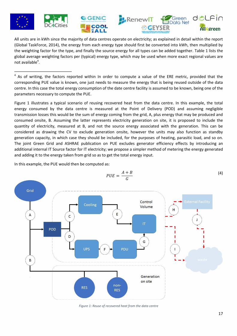
Figure 1 illustrates a typical scenario of reusing recovered heat from the data centre. In this example, the total

energy consumed by the data centre is measured at the Point of Delivery (POD) and assuming negligible

transmission losses this would be the sum of energy coming from the grid, A, plus energy that may be produced and

consumed onsite, B. Assuming the latter represents electricity generation on site, it is proposed to include the

quantity of electricity, measured at B, and not the source energy associated with the generation. This can be

considered as drawing the CV to exclude generation onsite, however the units may also function as standby

generation capacity, in which case they should be included, for the purposes of heating, parasitic load, and so on.

The joint Green Grid and ASHRAE publication on PUE (The Green Grid / ASHRAE, 2013) excludes generator efficiency

effects by introducing an additional internal IT Source factor for IT electricity; we propose a simpler method of

metering the energy generated and adding it to the energy taken from grid so as to get the total energy input.

In this example, the PUE3 would then be computed as:

(4)

Figure 1: Reuse of recovered heat from the data centre

Heat recovered by the data centre, H, may represent either hot air or water that is being fed into a heat pump and

further used by an external facility such as a nearby greenhouse, or the local/district heating grid. Based on ERF’s

definition by Equation (2), its value would then be:

(5)

with denoting the energy source weighting factor.

3 In this example, we assume the more advanced PUE category (3), where the IT load is measured at the IT equipment input.

17

All units are in kWh since the majority of data centres operate on electricity; as explained in detail within the report

(Global TaskForce, 2014), the energy from each energy type should first be converted into kWh, then multiplied by

the weighting factor for the type, and finally the source energy for all types can be added together. Table 1 lists the

global average weighting factors per (typical) energy type, which may be used when more exact regional values are

not available4.

4 As of writing, the factors reported within In order to compute a value of the ERE metric, provided that the

corresponding PUE value is known, one just needs to measure the energy that is being reused outside of the data

centre. In this case the total energy consumption of the date centre facility is assumed to be known, being one of the

parameters necessary to compute the PUE.

Figure 1 illustrates a typical scenario of reusing recovered heat from the data centre. In this example, the total

energy consumed by the data centre is measured at the Point of Delivery (POD) and assuming negligible

transmission losses this would be the sum of energy coming from the grid, A, plus energy that may be produced and

consumed onsite, B. Assuming the latter represents electricity generation on site, it is proposed to include the

quantity of electricity, measured at B, and not the source energy associated with the generation. This can be

considered as drawing the CV to exclude generation onsite, however the units may also function as standby

generation capacity, in which case they should be included, for the purposes of heating, parasitic load, and so on.

The joint Green Grid and ASHRAE publication on PUE excludes generator efficiency effects by introducing an

additional internal IT Source factor for IT electricity; we propose a simpler method of metering the energy generated

and adding it to the energy taken from grid so as to get the total energy input.

In this example, the PUE would then be computed as:

(4)

Figure 1: Reuse of recovered heat from the data centre

18

Table 1: Global average source energy weighting factors (Source: (Global TaskForce, 2014))

Energy type Weighting factor

Electricity 1.0

Gas (Natural gas) 0.35

Fuel oil 0.35

Other fuels 0.35

District chilled water 0.4

District hot water 0.4

District steam 0.4

As already implied by the discussion so far, this metric is data centre centric. In this sense, therefore, one does not

need to include in the computations pertaining to this metric the waste as a result of heat reused by the external

facility, J. That being said, one should ensure in advance that the business case for reusing recovered energy outside

the data centre’s premises is economically viable and environmentally sustainable: the resulted system’s total

energy consumption should be less when reusing energy.

In the remainder of this section we provide details on measurement points, metering equipment and assumptions,

along with guidelines on how to adequately identify a baseline scenario and possibly necessary adjustments. The

latter would be as part of the exercise to better capture, understand and analyse the energy recovered strategies

put in place along with opportunities for further improvements.

2.5.2.2 Baseline identification and calculation

To compute ERE no baseline identification is needed. However, an important step towards assessing the added value

of energy recovered from the data centre involves comparing the metric’s values between two different periods of

time. Such a comparison would then be made between the value over the period before implementing the measures

to recover energy, namely baseline, and the period following once improvements have been applied.

Baseline scenario must be representative of a typical operational period, normally being a year as thermal needs are

seasonal. Therefore, the base-year conditions refer to the knowledge base of the state of various data centre aspects

Heat recovered by the data centre, H, may represent either hot air or water that is being fed into a heat pump and

further used by an external facility such as a nearby greenhouse, or the local/district heating grid. Based on ERF’s

definition by Equation (2), its value would then be:

(5)

with denoting the energy source weighting factor.

All units are in kWh since the majority of data centres operate on electricity; as explained in detail within the report,

the energy from each energy type should first be converted into kWh, then multiplied by the weighting factor for the

type, and finally the source energy for all types can be added together. Table 1 lists the global average weighting

factors per (typical) energy type, which may be used when more exact regional values are not available.

Table 1 are in line with industry normal values, defined by The Green Grid, and due for inclusion in an updated version of the ERE definition document. It should be noted, however, that other European directives, particularly the Energy Performance of Buildings Directive (EPBD), utilise a different format, termed Primary Energy Factors. Whereas source energy factors use grid electricity as the base unity value (=1), primary energy factors use fossil fuel = 1, with electricity varying depending on grid electricity makeup.

19

during 12 months preceding the decision to deploy and use energy reuse infrastructure. In order to evaluate the

benefits of heat recovery, or changes to heat recovery, it is necessary to establish a baseline. This will require

gathering data over a range of operating conditions: IT loading, ambient weather conditions (seasonal variation) and

heat sink variations in load, temperature and flow, which is representative of the intended operating envelope.

Ideally this would involve at least 12 months with stable operating loads; in practice this may be difficult to attain

and a pragmatic approach should be adopted. For example, where heat recovery is considered beneficial during the

winter months only (heating season), then data from September – April may be considered adequate.

In the following, we divide this knowledge set into two categories, one pertaining information critical to enabling

accurate identification of the data centre’s baseline conditions and a second one, related to information that could

prove to be useful for enabling more fine-grained baseline identification, however affecting only slightly the resulting

baseline profile.

Collection and analysis of such data may allow us to compare variations in the ERE metric between these two

periods of time, eliminating to the degree possible the distortion effect on energy consumption introduced by such

variations – as already discussed in section 2.5.2.3.

The underlying assumption is that a data centre operator will normally be familiar with the main parameters that

affect data centre energy consumption. A detailed, orientative list is presented below, including the most common

parameters that relevantly affect data centre energy consumption, which would be mandatory to collect:

Electrical meter data, preferably for short time intervals (between 15 minutes and 1 hour, being every 30

minutes a good approach) for all factors necessary for PUE, ERE, and ERF calculation

Heat flow data across control volume: Medium, Humidity (for air), Flow, and Flow and Return Temperatures

Temperatures of IT Whitespace (CRAC/CRAH inlet and delivery) and Ambient and Heat sink

Confirmation that there has been no significant change in cooling plant configuration or operating

philosophy over the baseline period

A lighting levels investigation

A detailed report on the number and (static) energy characteristics of IT equipment (both for computing,

networking, and storage purposes) along with the respective energy consumption measurements, wherever

available

A detailed report on the number, and (static) energy characteristics of non-IT equipment (HVAC, lighting, and

so on) along with the respective energy consumption measurements, wherever available

A record of the temperature setting of cooling equipment

A report of the number, type and (static) energy characteristics of energy-reuse devices

A record of the number of working days and hours for each month of the year

A summary of detailed weather and climatic data for each month of the year

A report on the number, type, position and error of metering devices

A record of energy-efficiency techniques in place

In addition to these fundamental sets of data, the following pertain to information that could prove to be useful for

fine-tuning the data evaluation for the baseline identification if available, but are considered as too costly or too

hard to obtain;

More fine-grained reports regarding IT consumption behaviour of the various fundamental IT equipment

elements (CPU, RAM, HDD, Routers, Switches). In case a DCIM is used for monitoring and controlling the DC,

this information will most probably be available and should be used to identify the baseline.

20

More fine-grained reports of the components of the HVAC equipment (air conditioning, heating, lighting,

and so on) if the installation of a sufficient number of meters is not considered too costly, or a monitoring

framework is in place.

Bearing in mind the connection of this metric to PUE, for the aforementioned measurable entities, the sampling

period for measurements pertaining to dynamic parameters should be the same for both metrics. The base-year

energy use is metered at POD of Figure 1 spanning at least a 12-month period5. The base-year energy reuse is

metered at point H of Figure 1 spanning the same period as the one defined for the case of base energy use.

The base-year energy data should be analysed as follows. A mathematical model (e.g. linear regression) shall be

applied on representative period energy use and demand, IT load, metering period length, and degree days. The

latter shall be derived by third party information providers. Correlation of weather with energy demand, supply and

use is expected to be identified.

Benefits along with potential improvements derived from energy reuse will be determined under post-retrofit

conditions.

2.5.2.3 Baseline adjustments in case of anticipated changes

Baseline adjustments are needed to bring base-year energy use to the conditions of the post-retrofit period. The

method to measure and verify should be broadly in accordance with IPMVP Option C. Nevertheless, since formula (3)

is suggested to be used, then and bearing in mind that we measure PUE (IT energy consumption), the IPMVP Option

will be a mix of C and B.

2.5.2.3.1 Routine Adjustments

2.5.2.3.1.1 Electricity Consumption

At least, the electricity consumption is expected to be affected by the number of operating days and the weather. As

result, the following routine adjustments are normally needed:

The cooling equipment consumption may vary depending on the ambient temperature. Appropriate

adjustments should be made, based on manufacturer’s sheets.

The electricity consumption of air-conditioning and heating facilities should be adjusted to ambient

temperature based on manufacturers’ specifications.

2.5.2.3.1.2 Thermal Energy Waste

The waste heat may be used either to “heat” or “cool” external facilities. Adjustments on thermal energy waste may

be needed with respect to the number of operating days and hours, as well as the ambient temperature. Such

adjustments may be conducted following the specifications of the IT equipment manufacturers.

2.5.2.3.2 Electricity Demand

Adjustments on electricity demand may be needed, since the ambient temperature and daylight hours affect the

cooling, heating and lighting demand within the data centre.

In the cases that IT services offered to the customers have a relevant variation from year to year adjustments should

be applied.

2.5.2.3.2.1 Thermal Energy Demand

N/A

5 Ideally, integral multiples of 12-month periods (12, 24, 36 months, and so on) should be considered, in order to alleviate the

effects of seasonal DC workload variations.

21

2.5.2.3.3 Non-routine Adjustments

Procurement of new equipment during the post retrofit period raises the need for non-routine adjustments. The

new equipment may refer to IT (CPU, RAM, HDD, and networking devices), non-IT (cooling equipment), and facilities

(air-conditioning units, heating, and lighting). The adjustments should include calibrating the potential extra energy

consumption to the base-year one, referring to manufacturers’ factsheets on energy consumption.

2.5.2.4 Measurement boundaries determination & metering points

As already mentioned for this metric, being data centre centric, is not within scope to take into account whether an

equipment outside of the data centre’s premises is efficient or not. To that end, Coefficient of Performance (COP) of

external to the data centre heat pumps should not be considered. The energy reused should be measured exactly at

the point where it leaves the CV of the data centre. Nevertheless, the system’s total energy consumption should be

less when reusing energy.

On the other hand, cases where waste heat may be used, internally, to preheat generators for data centres

electricity production is also out of scope of ERE. In addition, electrical energy stored onsite for later use, including

possibly provision to external facilities, is considered out of scope of this metric, since stored energy is already

accounted for when measured at POD and in this context cannot be considered energy recovered.

2.5.2.4.1 Total energy consumption

Both the base-year and post-retrofit energy use for Equation (3) is taken directly from the metering equipment at

POD of Figure 1 without adjustment. Same guidelines as the ones related to PUE computation are to be followed.

2.5.2.4.2 Energy Reuse

Similarly both the base-year and post retro-fit energy reuse for Equation (3) is taken directly from the metering

equipment at point I of Figure 1 without adjustment.

2.5.2.5 Metering equipment desired characteristics/capabilities (HW / SW)

Metering equipment should be able to track kWh from the desired circuit.

The output from the main metering options should be made available on a web portal for ease of use and for easy

dissemination of information.

The data capture can be from:

existing ‘micro’ meters already in situ where the data is sent via the communication unit to the web portal;

new CT clamps on wiring linked to communication unit which will feed the web portal; and

temporary data loggers with CTs around specific circuit wiring and data caught locally and then uploaded.

2.5.2.6 Metering equipment commissioning procedure

2.5.2.6.1 Electricity

The DC circuitry should be fully analysed.

A plan of what circuits to be measured should be assembled.

In order to ascertain the most basic KPI (EnPI), PUE, and continuing with the assumption of the more advanced PUE

category, a meter is required at POD and at (G), the latter denoting the point of measurement for the energy

consumed by the IT equipment6, as shown in Figure 1. Additional metering will add to the complexity of data

obtained and help with the other KPIs.

6 For details on PUE measurement, please refer to (ISO/IEC JTC 1/SC 39 PUE, 2015).

22

It may be necessary to change some circuitry so that all the cooling, say, is captured on the one meter. If this is not

possible, then a schematic of the system should be drawn up and additional meters placed so as to capture all of the

necessary data for that specific energy use. Careful consideration must be taken so that energy is not missed nor

counted twice as this will cause significant problems with calculations.

2.5.2.6.2 Thermal

It will be necessary to capture the quantity, namely the volume, and quality, the temperature, of air being exhausted

or water being transferred. As such, meters other than kWh will have to be employed.

Flow meters will be necessary to calculate the volume. These will produce an output that should be captured by the

main monitoring system and sent via the communication unit to the web-portal.

In addition to the volume, the temperature of the air (both inside the data centre and ambient external) or the

water, will have to be captured. In particular, for water systems flow and return temperatures will be required.

In addition, one should record ambient temperature, air exhaust from data centre, and temperature of heated space

or district heating circuit.

Again, this information should be captured by the main data-capture system and sent via the communication unit to

the web-portal.

2.5.2.7 Metering assumptions

Energy lost through the fabric of the building is ignored and not measured. Steps to minimise these should be taken,

but not measured.

Capture of the quantity of air and its temperature will allow the calculation of the energy that the air contains. It will

be necessary to elaborate how this should be done.

2.5.2.8 Metering sampling frequency

The data sampling frequency should facilitate calculations to give an accurate picture of the energy use in the data

centre. If the data centre energy use and processing speeds are very constant, then low sample rates may suffice.

However, if very rapid changes are observed, then a higher sampling rate may be required.

For example, in the data centres that Google operate, they collect these types of data every second. As such they

have 86,000 data points for every meter every day. This level may be too fine for some applications.

However, hourly data points may be too coarse. So a suitable medium position may be required.

A sample rate of, for example, between every 30 seconds and every 10 minutes will probably allow a good data set

from which to first start. Adjustments up or down from this may be necessary after the first tranche of data is

analysed. In general, sampling frequency should not be too short so as to avoid noise from actions of control

systems. Aggregating to periods of 1 hr or 1 day for modelling and metric calculation could be a good compromise.

Typical values of sample rate per parameter are listed in Table 2.

Table 2: Typical values of sample rate per parameter.

Level of Granularity Parameter Interval (min*)

Server room (non – IT)

Air temperature 5 – 10

Chilled water flow rate 0.5 – 1

Chilled water temperature 5 – 10

Relative humidity 5 – 10

Server room (IT) CPU utilisation % 0.5 – 1

23

Networking utilisation7 % 0.5 – 1

Storage utilisation8 % 0.5 – 1

Server room exit Air flow rate 0.5 – 1

Air temperature 5 – 10

Electricity

Main incomer 0.5 – 10

UPS 0.5 – 10

Server room incomer 0.5 – 10

General Degree days cooling 1 day

Outside dew point 1 hour

2.5.2.9 Metering duration (post-retrofit period)

The duration of the measurement should be at least over 12 months, or at least encompass both summer and winter

conditions. This will allow the analysis over a full cooling (and heating) season.

It will be preferable to allow 3 full years of data to show any annual trends. This will give a more robust result of the

system.

7 Current switching throughput / Max switching throughput

8 ((used storage capacity/maximum storage capacity) + (data transfer/max data transfer capacity))/2

24

3 Task 4.2 – Methodologies for new Metrics

The purpose of Task 4.2 was to define methodologies for new metrics selected by the Smart City Cluster

Collaboration during Task 3. Hence, the work for this task involved considering methodologies most suitable for use

by the cluster and extending known methodologies.

The methodologies hereby defined should be viewed as a first attempt in tackling the introduction of such a global,

environmental family of metrics for the data centre. As such, the document describes the proposed approach simply

as a step-by-step guideline the data centre operator may follow to measure the necessary parameters for computing

the selected metric(s). The project-members of the cluster will put this approach into practice during their pilot

trials. In doing so, insights will be obtained to refine the proposed methodology as necessary.

Metrics within Task 4.2 are classified into three categories:

Flexibility Mechanisms in Data Centres - Energy Shifting, including metrics such as Adaptability Power Curve

(APC), Adaptability Power Curve at Renewable Energies (APC_REN), and Data Centre Adapt (DCA)

Savings family of metrics including Primary Energy Savings (PE Savings), CO2 avoided emissions (CO2

Savings), and Energy Expenses (EES),

Renewables integration - Energy produced locally and Renewable usage with the Grid Utilization Factor

(GUF) metric.

3.1 Adaptability Power Curve

3.1.1 M & V Plan Scope and Metric Overview

The present section is aimed to provide the measurement and verification methodology for the APC metric, following the International Performance Measurement and Verification Protocol (IPMVP).

The APC metric belongs to the category of “Flexibility mechanisms in Data Centres: Energy shifting”, presented in “Cluster Activities Task 3” document (§2.2.1).

This metric assumes that an energy usage pattern is in place, to which the data centre must adapt to the greatest extent possible. The energy plan may be provided by an Energy Managing Entity within the Smart City or the Smart grid or by the DC itself, as a result of self-optimization policies. APC aims at measuring the degree of adaptation of the DC energy consumption to a planned energy curve.

APC is given by the following formula:

(1)

(2)

Where:

is the DC energy consumption in kWh;

is the planned energy in kWh;

is the individual time period

represents the sample size and

is the adjustment factor between and normalising the two energy consumption curves.

25

To specify better, the a priori defined cannot take into account possible changes in current conditions and the incurring variations in current . To eliminate the effect of these variations on the metric performance scales the planned energy at the level of the energy consumption , i.e. the two curves must subtend the same area in order to have the same total energy and be therefore comparable.

As derived from eq. (1), APC values are unit-less where 1.0 corresponds to full adaptation. The lower the adaptation between both curves is, the lower the value achieved for APC (very different curves can cause even APC negative values). In order to calculate the APC values, the planned and actual DC energy usage have to be provided; the former is calculated or provided, while the latter is measured.

3.1.2 Measurements


According to the formula aforementioned, the only parameter to be measured is the total energy consumption of

the data centre for each time interval in kWh. More information on the selected timeframe and the baseline

scenario is found within sections 3.1.2.2 and 3.1.2.3. For details on measurement points please refer to section

3.1.2.4.

is not measured, as its values are predetermined by the DC management or some other entity. and are

energy consumptions produced at the same time (simultaneous), i.e. is the energy consumed by the DC after

trying to adapt its consumption to the demand order (

It must be noted that, unlike other metrics, no independent variables/static factors are needed to be measured, as

only the profiles of the curves are compared.


Baseline is not applicable to this metric.


As no baseline is applicable to this metric, no adjustments are required.


Figure 2: Data Centre Control Volume and Measurement Points illustrates a general scenario of a data centre. The

total energy consumption of such a data centre is measured at the Point of Delivery (POD) and is the summation of

energy coming from the utility (A) plus energy generated onsite (B); both measurements are in kWh. This means that

all types of energy are considered, both primary (e.g. fuel for an onsite generation engine) and secondary, and

converted in electricity.

26

Figure 2: Data Centre Control Volume and Measurement Points

However, it is worth highlighting that particular cases in which the energy plan provided to the Data Centres does

not include onsite production could happen. For example, in the case that there is a restriction or a demand order

only for the electricity consumed from the grid. In that case, energy consumption to consider will have to be

measured at the meter from the utility (A).


All the required variables can be metered using permanent energy meters, installed on the metering points

highlighted in the previous paragraph. Those energy meters should comply with the following requirements.

- Meters range must be consistent with the metered variables range and these meters should allow a

consistent unit selection.

- Meters must be equipped with a communication module (Modbus RTU RS485 protocol or equivalent), must

be connected to a gateway that via Ethernet allows concentrating data that are stored in log files or in a

database. A properly sized storage system must be designed and installed and data must be available for the

next phase of analysis and verification. In this way, each meter, becomes a node of the network.

Meters must be equipped with the required auxiliary devices such as amperometric transformers, voltmetric

commutators, surge protectors and surge arresters.

- The choice of measurement boundaries and metering points must be performed from the Data Centre

perspective. Moreover meters and auxiliary devices must be chosen according to the supply voltage. For this

reason, LV point of measures must be preferred to MV point of measures, also due to lower metering costs.

Measurement errors (defined by the HW’s accuracy classes), connections, communication protocols and networking

must be compliant with the existing standards (ANSI, IEC, IEEE, CEI EN) and national regulations.


The commissioning process assumes that owners, programmers, designers, contractors, operations and

maintenance entities are accountable for the quality of their work. Commissioning process includes several

27

procedures that are required in order to ensure the adequacy and the degree of precision required for the quality of

measurement and the product safety.

Once the measurement system is installed, a test procedure must be performed. During this procedure, once the

meter settings are set, the measure collected by the installed meter is compared with the measure collected through

a portable configured meter. The test procedure must not be confused with the calibration procedure performed by

the manufacturer. The test procedure includes the test of the communication channels (speed and reliability) and

the sampling time.

Together with the test procedure a maintenance procedure is required. The key tests required are:

- Every time the gateway does not communicate with the storage system or one or more nodes do not

communicate with the gateway it is necessary to check and solve the problems in due time.

- Periodically (once a year) it is important to inspect the measurement equipment and repeat the calibration

procedure.

- Every time hardware changes occur, the compliance between the meter range and the physical variable

range must to be checked and guaranteed.

If the commissioning procedure is workmanlike performed a maintenance procedure is not indispensable


As APC is based on comparing the total energy consumption of a DC to acomputed (optimal) energy consumption

curve, the main assumptions will be that Sections 3.1.2.1, 3.1.2.4 and 3.1.2.5 provide all the necessary information

(metering equipment, location) to measure the total energy consumption of the DC. All meters are assumed to be

calibrated, commissioned and tested, so the energy consumption measurement values are accurate and rigorously

collected and the samples are representative. If these assumptions are not met, an analysis to detect which

measurements are being missed or are not being considered should be made, and a procedure to include them with

new equipment or with estimations must be applied, including quantifying all the uncertainties added in case of

estimating any consumptions.

In case of changes in the metering equipment (including removal or plain change) during the sampling period, it is

assumed that the M&V plan describes all the specifications and calibration requirements and locations of the

metering equipment in order to continue the close as possible to the same metering scenario.





The sampling frequency will have dependency on hardware and software requirements (granularity of the meters,

data storage limitations, SCADA or Software limitations etc.); to capture the energy consumption pattern a

frequency in the order of minutes should be considered. Low measuring frequencies introduce the risk of not

capturing energy consumption peaks, reducing the effectiveness of the energy consumption behaviour capturing. To

this end, a measurement every 1 to 5 minutes would be recommendable with a maximum period not exceeding 15

minutes. In any case, the optimal energy consumption behaviour calculation should follow the DC energy

consumption measurements period and vice versa, in order to avoid unnecessary, overhead computational and

metering load.

In practice, a measurement period of 15 minutes (96 measures per day) is a good approach, providing a clear picture

of the daily energy pattern consumption of a DC, being adequate for the creation of different energy baselines.


The pre- and post- implementation period should be measured with a similar period length and conducted using the

same procedure (equipment, sensor location, etc.).

28

As energy consumption depends on weather conditions, the measurements should include all the different seasons

and all different weather conditions: for this reason whole year duration is recommended. Similarly, variable DC

workload and usage patterns should be contemplated. For example, University or office building DCs will have

clearly less workload in summer or during holiday periods. Taking into consideration all the above, a post-retrofit

period of at least a year is the best option to capture DCs energy behaviour.

The minimum period must be one that sufficiently covers a wide range of weather and usage conditions. In this case

specific metering duration periods will be selected, depending on usage and location of the DC, in order to give a fair

representation of the DC behaviour.

3.1.3 Example Indicatively, Figure 3 presents an example calculation of the APC flexibility metric for a hypothetical DC. Specifically,

assuming that the measurement procedures described in the previous paragraphs were respected, Figure 3 depicts

the measured DC energy consumption , versus the planned energy consumption, for 6 consecutive time

intervals, i = 1,..,6.

In the example assumed, the adjustment factor equals

. Therefore, APC can be

calculated as follows:

(3)

Figure 3: DC energy consumption, and planned energy consumption, over time

29

3.2 Adaptability Power Curve at Renewable Energies

3.2.1 M & V Plan Scope and Metric Overview The present section is aimed to provide the measurement and verification methodology for the APCREN metric,

following the International Performance Measurement and Verification Protocol (IPMVP).

The APCREN metric belongs to the category of “Flexibility mechanisms in Data Centres: Energy shifting”, presented in

“Cluster Activities Task 3” document (§2.2.2).

This metric assumes that a renewable energy availability is provided, to which the data centre must adapt to the

greatest extent possible. The energy plan may be provided by an Energy Managing Entity within the Smart City or

the Smart grid or by the DC itself, as a result of self-optimization policies. APCREN aims at measuring the degree of

adaptation of the DC energy consumption to a planned renewable energy curve.

APCREN is given by the following formula:

(4)

(5)

where:

is the DC energy consumption in kWh;

is the available renewable energy (to be consumed) in kWh;

is the individual time period

represents the sample size and

is the adjustment factor between and .

Specifically, as accounts for all available renewable energy, its order of magnitude will generally be higher

than that of . The opposite is unlikely. In this course, allows the correlation of both variables providing

information - on the adaptability of the power curve - which otherwise would be suppressed by the difference in the

order of magnitude.

As derived from eq.(4), APCREN values are unit-less, where 1 corresponds to full adaptation. The lower the adaptation

between both curves is, the lower the value achieved for APCren (very different curves can result to negative APCren

values).

3.2.2 Measurements


According to the formula aforementioned the parameters to be measured are:

total energy consumption of the DC for each time interval i expressed in kWh;

total energy coming from renewable sources, taking into account both the onsite generation and the energy

purchased on meter at time instant i expressed in kWh. In the case of primary energy containing a

percentage of energy coming from renewable sources, the calculation of the absolute value of purchased

renewable energy should derive as the multiplication of this percentage with the total energy purchased.

For details on measurement points please refer to section3.2.2.4.

30


Baseline is not applicable to this metric.


Baseline is not applicable to this metric and therefore no baseline adjustment is required.


Figure 4: DC Control Volume and Measurement Points illustrates a general scenario of a DC. The total energy

consumption of such a DC is measured at the Point of Delivery (POD) and it would be the summation of energy

coming from the utility (A) plus energy generated onsite (B); both measurements would be in kWh. This means that

all types of energy are considered, both primary and secondary, and converted in electricity.

The energy coming from renewable sources is the summation of energy produced locally BonsiteRes plus the

percentage, if any, purchased from the utility.

Figure 4: DC Control Volume and Measurement Points








database. A properly sized storage system has to be designed and installed and data must be available for

the next phase of analysis and verification. In this way, each meter, becomes a node of the network.

31






Finally, measurement errors (defined by the HW’s accuracy classes), connections, communication protocols and

networking must be compliant with the existing standards (ANSI, IEC, IEEE, CEI EN) and national regulations. The

requirements specified in these standards and regulations have to be considered as minimum values for the

meters under normal working conditions. For special application, higher constraints might be necessary and

should be agreed between the user and the manufacturer.










the sampling time.


Every time the gateway does not communicate with the storage system or one or more nodes do not


Periodically (once a year) it is important to inspect the measurement equipment and repeat the calibration

procedure.

Every time hardware changes occur, the compliance between the meter range and the physical variable


If the commissioning procedure is workmanlike performed a maintenance procedure is not indispensable.


As APCREN is based on comparing the total energy consumption of a DC to the total energy provided by renewable

energy sources (RES availability from the grid and local generation), the main assumptions will be that Sections

3.2.2.1, 3.2.2.4 and 3.2.2.5 provide all the necessary information (metering equipment, location) to measure the

total energy consumption of the DC. All meters are assumed to be calibrated, commissioned and tested, so the

energy consumption measurement values are accurate and rigorously collected and the samples are representative.

For renewable energy availability curve the assumptions will be that the curve is produced taking into consideration

all the onsite renewable power systems that feed the DC, and that the energy provided by renewable systems has

been accurately measured. A procedure to measure the grid energy share that comes from renewables (RES

certificate) shall be established with a timeframe in the same order of the measurements provided by

measurements in the onsite installation.

If these assumptions are not met, an analysis to detect which measurements are being missed or are not being

considered should be made, and a procedure to include them with new equipment or with estimations must be

applied, including quantifying all the uncertainties added in case of estimating any consumptions.

32






data storage limitations, SCADA or Software limitations etc.); to capture the energy consumption pattern a




minutes.

In the case of renewable energy production, a higher measurement frequency is needed to cope with the

intermittent nature of the RES production. Indicatively, solar or wind energy production are extremely variable; a

recommending measurement period would be 1 minute. In any case, the measurements period regarding RES

should follow the DC energy consumption measurements period and vice versa, in order to avoid unnecessary,

overhead computational and metering load.


of the daily energy pattern consumption of a DC, being adequate for the creation of different energy baselines. For

renewable energy production measurements, 15 minute are too high and higher sampling rates in the order of 30

seconds to 1 minute would be necessary to capture the renewable energy contribution.

Summing up, a recommendable sample time would be 1 minute and the sample time shouldn’t be higher than 15

minutes.





and all different weather conditions: for this reason whole year duration is recommended. Similarly, variable DC





specific metering duration periods will be selected, depending on usage and location of the DC, in order to give a fair

representation of the DC behaviour.

3.2.3 Example Indicatively, Figure 5 presents an example calculation of the APC_REN flexibility metric for a hypothetical DC.

Specifically, assuming that the measurement procedures described in the following paragraphs have been respected,

Figure 5 depicts the measured DC energy consumption, , versus the available renewable energy, at 6

consecutive time intervals, i = 1,..,6.


Therefore, can

be calculated as follows:

(6)

33

Figure 5: DC energy consumption, E_DC and the available renewable energy, E_Ren over time

3.3 Data Centre Adapt

3.3.1 M & V Plan Scope and Metric Overview

This section presents the measurement and verification plan pertaining to the newly proposed metric Data Centre Adapt (DCA). This metric provides information on how much the energy profile of a data centre has shifted from a baseline energy consumption after the implementation of flexibility mechanisms has taken place. By flexibility mechanisms we refer to strategies, policies or in general sets of actions, such as employing workload management techniques, in an effort to adapt the data centre’s energy consumption as much as possible to a planned energy curve. Ideally, the planned energy curve is one that represents running the data centre in a more energy efficient mode. This metric measures the change of the energy consumption curve.

It is important to distinguish DCA from a related energy shifting metric, namely APC. The latter compares a planned curve, suggested for example by an energy manager in order to modify the data centre’s energy consumption according to energy optimizations, constraints, or both, and its actual final consumption, modified in an effort to follow the suggested energy curve. The information then provided by this indicator is the data centre’s capability to adapt its consumption as in a demand response paradigm. Although the planned energy curve is determined previously, information given by both curves belongs to the same time period.

Conversely, DCA provides information about the flexibility that has been achieved after implementing actions to

adapt the data centre’s energy consumption during certain periods of time to energy profiles that are selected as

more advantageous, if compared with the energy profiles operating before. The reason for the changes will normally

be the adaptation of the consumption to a planned power curve (devised autonomously or provided by a smart grid

15 18

13 19 18 17

10

19

98

83

18 22

0

20

40

60

80

100

120

1 2 3 4 5 6

Ener

gy C

on

sum

pti

on

(M

Wh

)

Time Period i

EDC ERen

34

authority). However, this metric provides no information about the accuracy level of this adaptation; it rather

focuses on the degree of flexibility achieved due to the modifications in the operation approaches of the data centre.

These two curves, necessary to compute DCA, are not simultaneous in time. Therefore, information on the data

centre before and after implementing changes is required.

The equation below denotes the general mathematical formula to compute this metric:

(7)

is a scaling factor to render comparable the involved energy consumption curves. In particular, due to the inclusion of the flexibility mechanisms, variations in the global energy consumption may occur. Moreover, variations due to services provided, outside temperature, and so on, may appear as baseline and real consumption are not simultaneous in time; baseline measurements constitute the energy consumption pattern of a data centre before implementing actions or changes in SW or equipment that imply variations in this pattern (flexibility). Thus, it is necessary to normalise the resulted curves in order to compare the profile of energy consumption without introducing this distortion. The equation below provides the mathematical formula to compute this factor:

(8)

where:

denotes the data centre’s real energy consumption in kWh at a given point in time, i. This is the energy consumption after the implementation of flexibility mechanisms has taken place.

denotes the data centre’s baseline energy consumption in kWh at a given point in time, i. This is the energy consumption before the implementation of flexibility mechanisms. Baseline energy consumption profiles must be obtained by analysing and modelling the energy consumption of the data centre before the actions provided by flexibility mechanisms have been implemented (see section 3.3.2.2 for details).

represents the sample size.

The numerator within the formula for DCA represents the cumulative, absolute error between and , while the denominator represents the summation of over the whole sample, in other words the area below the baseline curve.

A DCA value equal to 1 means that the curve has not changed. A high flexibility of the consumption curve will imply a lower value for DCA (very different curves can cause even DCA negative values).

3.3.2 Measurements


According to the formula aforementioned, the only parameter to be measured is the total energy consumption of

the data centre at a given point in time in kWh. More information on the selected timeframe and the baseline

scenario is found within sections 3.3.2.2 and 3.3.2.3. For details on measurement points please refer to section

3.3.2.4.


The baseline is evaluated experimentally measuring power values at points A and B of the diagram as well as the

Point of Delivery (POD) of the DC. Given that the DC can be considered as a “black box”, no other measurements are

needed in this case. To perform the baseline evaluation an appropriate value for Δt must be selected.

We are dealing here with a metric in which the variation as a function of time is of particular importance. Typical daily profiles must therefore be measured. To do so, frequent measures of Energy consumed must be taken to

35

determine the baseline scenario. Obviously, the same frequency will be adopted to obtain the measures in the “real” scenario, i. e. after actions/changes in SW or equipment that imply variations have taken place. For practical purposes Δt = 15 min seems adequate (choice currently being used in DC4Cities). Daily profiles must be collected under different operational conditions of the DC. Effectively, profiles can exhibit significant variations depending on seasonal effects (winter/summer), workload changes (i.e. working day/weekend, specific deadlines, etc.). In order to assess correctly the Baseline it will be therefore necessary to create a set of typical profiles. Requisites and characteristics of the set must be determined for the specific DC under study.


For this metric Baseline adjustment is not needed, due to the usage of the scaling factor .


Figure 6 illustrates a typical scenario of a data centre. The total energy consumption of such a data centre is

measured at the Point of Delivery (POD) and it is the summation of energy coming from the grid (A) plus energy

generated onsite (B); both measurements are in kWh. This means that all sources of energy are considered and

converted in electricity. For details on conversion factors please refer to the cluster report pertaining to the metric

“Primary Energy Savings”.

Figure 6: Data Centre Control Volume and Measurement Points








36

database. A properly sized storage system must be designed and installed and data must be available for the

next phase of analysis and verification. In this way, each meter, becomes a node of the network.







networking must be compliant with the existing standards (ANSI, IEC, IEEE, CEI EN) and national regulation. The

requirements specified in these standards and regulations have to be considered as minimum values for the

meters under normal working conditions. For special application, higher constraints might be necessary and

should be agreed between the user and the manufacturer.










the sampling time.


- Every time the gateway does not communicate with the storage system or one or more nodes do not


- Periodically (once a year) it is important to inspect the measurement equipment and repeat the calibration

procedure.

- Every time hardware changes occur, the compliance between the meter range and the physical variable


If the commissioning procedure is workmanlike performed a maintenance procedure is not indispensable.


As DCA is based on comparing the total energy consumption of a DC to its energy consumption during a previous

time period, the main assumptions will be that Sections 3.3.2.1, 3.3.2.4 and 3.3.2.5 provide all the necessary

information (metering equipment, location) to measure the total energy consumption of the DC. All meters are

assumed to be calibrated, commissioned and tested, so the energy consumption measurement values are accurate

and rigorously collected and the samples are representative. If these assumptions are not met, an analysis to detect

which measurements are being missed or are not being considered should be made, and a procedure to include

them with new equipment or with estimations must be applied, including quantifying all the uncertainties added in

case of estimating any consumptions.

For Section 3.3.2.2, the assumption will be that all the different baselines and profiles necessary for measurement

and verification process are defined. As these baselines will be used to calculate the energy savings after the energy

saving process it is important that the consumption behaviour of the DC is completely addressed.




37



data storage limitations, SCADA or Software limitations etc.), to capture the energy consumption pattern a




minutes.


of the daily energy pattern consumption of a DC, being adequate for the creation of different energy baselines.





and all different weather conditions: for this reason, a whole year duration is recommended. Similarly, variable DC





specific metering duration periods will be selected, depending on usage and location of the DC, in order to give a

fair representation of the DC behaviour.

3.3.3 Example Indicatively, Figure 7: Energy consumption, both real and baseline presents an example calculation of the DCA

flexibility metric for a hypothetical DC. Specifically, assuming that the measurement procedures described in the

previous paragraphs were respected, Figure 7: Energy consumption, both real and baseline depicts the data centre’s

real energy consumption in kWh and the data centre’s baseline energy consumption in kWh

for 7 consecutive time intervals, i = 1,..,7.


. Therefore, DCA can

be calculated as follows:

(9)

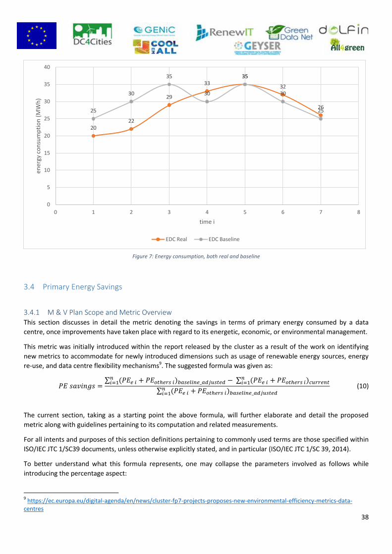
38

Figure 7: Energy consumption, both real and baseline

3.4 Primary Energy Savings

3.4.1 M & V Plan Scope and Metric Overview This section discusses in detail the metric denoting the savings in terms of primary energy consumed by a data

centre, once improvements have taken place with regard to its energetic, economic, or environmental management.

This metric was initially introduced within the report released by the cluster as a result of the work on identifying

new metrics to accommodate for newly introduced dimensions such as usage of renewable energy sources, energy

re-use, and data centre flexibility mechanisms9. The suggested formula was given as:

(10)

The current section, taking as a starting point the above formula, will further elaborate and detail the proposed

metric along with guidelines pertaining to its computation and related measurements.

For all intents and purposes of this section definitions pertaining to commonly used terms are those specified within

ISO/IEC JTC 1/SC39 documents, unless otherwise explicitly stated, and in particular (ISO/IEC JTC 1/SC 39, 2014).

To better understand what this formula represents, one may collapse the parameters involved as follows while

introducing the percentage aspect:

9 https://ec.europa.eu/digital-agenda/en/news/cluster-fp7-projects-proposes-new-environmental-efficiency-metrics-data-

centres

20 22

29

33 35

32

26 25

30

35

30

35

30

25

0

5

10

15

20

25

30

35

40

0 1 2 3 4 5 6 7 8

ener

gy c

on

sum

pti

on

(M

Wh

)

time i

EDC Real EDC Baseline

https://ec.europa.eu/digital-agenda/en/news/cluster-fp7-projects-proposes-new-environmental-efficiency-metrics-data-centres


39

(11)

where,

denotes the total energy consumed by the data centre, in terms of primary energy, measured during

period as a summation of discrete intervals10 in time, while

denotes the total energy that would have been consumed by the data centre, also in terms of

primary energy, during the “same” period provided that conditions would have remained the same as in the

baseline scenario.

Total energy in this case takes into consideration not only the energy consumed by the data centre in form of

electricity, , but also energy consumed in any other form, , such as for example chilled water for

cooling purposes:

(12)

All parameters are in primary energy terms with the unit of measurement being the kWh.

The selected period may depend on the type of the data centre in question, the characteristics of its business

model, the type of the intervention and so forth. On a business as usual scenario, one should opt for a period equal

to a year – so as to take into account a statistical average of the typical behaviour of a data centre, including end-

user’s consumption patterns, along with variations pertaining to environmental conditions, such as outside

temperature, sun and wind intensity. However, for practical reasons and for the purposes of the projects within the

cluster this period may be adapted to fit the general planning.

For details on the selection of the timeframe along with information on the baseline scenario please refer to

sections 3.4.2.2 and 3.4.2.3.

It should be noted that this metric along with the related ones on CO2 emissions and economic expenses are meant

to be global metrics11; as such the data centre is therefore viewed as a black box. Both of these metrics are actually

variants of the one pertaining to the primary energy, adjusted with appropriate factors.

More information on the related metrics and their measurement and validation plan is found within their respective

reports.

In the following we provide details on the methodology related to measurement, analysis, and reporting of this

metric.

3.4.2 Measurements


Based on the formula aforementioned and in line with the concept of treating the data centre as a black box the

parameters to be measured are:

10

Discrete interval will depend on the goal pursued to compute the metric, and may vary from a time interval equal to 15 minutes or 1 hour to a time interval of 1 week, month or year. 11

In case the data centre operator is interested in evaluating improvements pertaining to a subsystem instead (such as primary

energy savings of the cooling system), the methodology defined within this section may be applied; naturally the measurement

boundaries would have to be adjusted accordingly.

40

Total energy taken by the grid, measured at the meter for each interval, and consumed during a pre-selected

period of time ; and

Total energy produced and consumed on site for immediate and own consumption (back-up generators,

solar panels, natural gas for absorption chillers, and so on) for each interval.

For details on baseline scenario specifications please refer to sections 3.4.2.2 and 3.4.2.3, while for information

related to measurements points to section 0.


The baseline is evaluated experimentally measuring energy values at points as indicated within section 0 Given that

the data centre can be considered as a “black box”, no other energy measurements are needed in this case.

To perform the baseline evaluation an appropriate value for must be selected. In principle, we are dealing with an

aggregated value, and therefore corresponds to a relatively long period, typically 1 year. Metering sampling

frequency has to be the same in both current and baseline scenarios (see section 3.4.2.8).

In practice it may not be always possible to carry out the determination of a baseline scenario throughout a year.

This can be true, for example, in cases where measurements are bound to a shorter period such as during pilots or

an energy audit to evaluate the feasibility of a business case. Under such conditions, the baseline scenario may be

simulated by assessing the value of the energy consumption for a set of “typical days” and then projecting these on a

one-year period. Requisites and characteristics of the set must be determined for the specific data centre under

study.

Daily values building up the typical behaviour must be collected under different operational conditions of the data

centre, including also variations in energy supply patterns. This is because significant variations due to seasonal

effects (winter/summer), workload changes (for example working day/weekend, specific deadlines, and so on), and

different hourly prices depending on the day/month may occur.


A need for baseline adjustment arises when some “external factor” introduces a change in the baseline value.

External factors of practical importance are:

• substantial changes in the equipment, IT, power, cooling or otherwise, of the data centre;

• refurbishment/renovation of the premises where the data centre is located;

• changes in environmental parameters (temperature, relative humidity, and so on);

• business changes, for example partnerships, mergers, acquisitions, opening of new markets and activities;

• significant changes in workloads, workload distribution, or both.

It is worth distinguishing between routine and non-routine adjustments.

Routine adjustments are those that would be done regularly, for example, due to changes in weather conditions or

IT workloads. Most of such external factors introduce non-linear effects in the formulas. For instance, increases in

the total workload of a data centre do not imply corresponding proportional increases in the energy consumption.

As an example, the simple routine adjustment of the baseline through a multiplying factor, therefore a relation

obtained as a linear regression, as in Equation (13), is hardly ever possible:

(13)

In general, it is therefore not possible to estimate “theoretically” values for the parameters above; at least not

without performing a new experimental assessment of the baseline. In certain specific cases it might appear possible

to perform such an estimate, but a general operational rule cannot be given and the calculation of the adjustment

will have to be performed on a case-by-case basis.

41

A non-routine adjustment would occur due to an isolated event, for example, an increase of the total DC surface

(new equipment). In this case, a new mathematical model has to be performed. Following the previous example, a

new linear regression would have been to be calculated and this new formula would be used to adjust baseline:

(14)


Figure 8 illustrates a typical scenario of a data centre. The total energy consumption taken by the grid is measured at

point A, for example with a meter close to the POD. For other forms of energy such as gas, fuel, or chilled water the

measurement is taken at the point of delivery of each source, for example as input to the non-RES element of Figure

8, while for renewable generation onsite the energy produced and consumed is measured with a meter at the

output of the RES element.

All forms of available to the data centre energy must be considered in terms of primary energy; naturally in order to

consolidate the various sources, their value must be adjusted accordingly based on the Primary Energy Factors (PEFs)

as discussed in section 3.4.2.7.

Figure 8: Data Centre Control Volume and Measuring Points


All the required variables can be metered using permanent energy meters. They should be provided of a

communication protocol module such as for example ModbusRTU RS485 or equivalent. The measure error has to be

1% or lower (active energy).


Meter range has to be consistent with the variable range. Meters setup during commissioning should include

consistent unit selection. Meters calibration preferably should take place once a year.

42


By primary energy we refer to all energy forms as found in nature, which are used to generate the supply of energy

carriers, electricity being the most common of the latter. For both the nominator and denominator in the formulas

given by Equation (14), all forms of energy sources available to the data centre, such as electricity, gas and so on, are

taken into consideration. As already mentioned all sources are converted to primary energy terms; the unit of

measurement being the kWh12.

The purpose of the source energy conversion is to enable comparison of different forms of energy by data centres.

Since the majority of data centres operate with 100% electricity, the Harmonizing Metrics Task Force (Global

TaskForce, 2014) recommends energy factors weighted with respect to electricity. However, this does not allow for

any weighting between grid and locally generated electricity to produce comparable source energy measures. In

addition, converting all energy sources in primary energy terms has a real physical meaning, as electricity is energy

already transformed by either bulk or distributed generation and thus may introduce significant distortion related to

equipment performance efficiency, transportation losses, and so on.

For the conversion, appropriate and established conversion factors must be used, the so-called PEFs. However, there

is no unified approach in European regulations on how to calculate these factors (Molebroek, Stricker, & Boermans,

2011).

Generally speaking, for electricity this factor should represent "the average efficiency of all the power plants and the

probability of each of them in operation at a certain time minus the amount of electricity from renewable sources

and their probability plus the distribution losses" per country or region. Electricity has usually the highest primary

energy factor due to low efficiency of power plants which on average is around 35%. The calculation of such a factor

is very complicated, not to mention that in most cases exact details of the algorithm are not even publicly available.

As such it is always estimated and actually it seems political decisions have a large influence on the final value; in

other words it should be provided by the national or local governments.

Table 3 lists the PEFs of seven European countries for delivery of electricity to a building according to their national

building regulations. The PEF for the majority of countries is approximately 2.6.

Table 3: PEFs of seven European countries for delivery of electricity to a building (Source: (Molebroek, Stricker, & Boermans, 2011))

France Germany NL Poland Spain Sweden UK

PEF 2.58 2.60 2.56 3.00 2.60 2.00 2.92

However, these values are typically updated every few years; therefore one should always check with the local or

national authority for the most recent value. For example, in Germany the PEF for electricity was changed from 2.6

to 2.4 in 2014 (DIN V 18599-1) and is expected to change to 1.8 in 2016 with a factor of 1.2 as the target for the year

2020 (EnEV 2014 “Energy Saving Regulation in Germany”).

Moreover, this aggregated value has relevant seasonal variations, or even relevant variation within the same day.

Therefore, should one wishes to use this metric to also evaluate demand response scenarios, where flexibility

mechanisms are introduced in the data centre, electricity PEF may not be considered as a constant value; in this case

one may compute this factor for each while taking into account variations in the (local) electricity mix.

12

Energy is commonly measured in Btus (U.S. units) or kWh (metric units); for reference, the definition of a Btu, or British thermal unit, is the energy it takes to heat one pound of water by one degree Fahrenheit. Note that kWh, although it is typically used for electricity, is a unit of energy (not just electricity)—and can thus be applied to any fuel source.

43

On the other hand, an annual average should suffice when the KPI is used for other purposes. This would include, for

example, evaluating general energy efficiency scenarios such as retrofitting of cooling systems, replacing electric

heat pumps with absorption chillers, and so on.

includes an example of total weighting factors and that the weighting factors for general grid-delivered electricity

exceed 1. Primary energy weighting factors are given for largely or wholly renewable energy sources including wood

and on-site solar PV. As aforementioned, some of these factors can be variable, depending on the origin of the

source (e.g. coal from different compositions), the performance for each technology or the approach followed by

each country. includes an example of total weighting factors and that the weighting factors for general grid-delivered

electricity exceed 1. Primary energy weighting factors are given for largely or wholly renewable energy sources

including wood and on-site solar PV. As aforementioned, some of these factors can be variable, depending on the

origin of the source (e.g. coal from different compositions), the performance for each technology or the approach

followed by each country.

Table 4: Total primary energy weighting factors - delivered and exported energy. (Source: CEN: EN 15459 Energy Performance of buildings - Economic evaluation procedure for energy systems in buildings, 2007 (quoted in RenewIT D3.1 Metrics for Net Zero Data Centres)).

Form of energy supplied Non-renewable primary energy weighting factor

Gas 1.05

Oil 1.05

Coal 1.05

Grid electricity

2.3

Grid electricity by hydraulic power plant

0.5

Liquid biomass and biogas 0.5

Wood 0.05

District heating (based in gas fired boiler plant)

1.3

District cooling 1.3

Solar PV on site 0

Thermal solar on site 0

Cogeneration unit electricity (non-renewable fuel)

1.6

PV electricity 1.6

Cogeneration unit electricity (non-renewable fuel)

2

PV electricity 2

Cogeneration unit electricity 2.5

PV electricity 2.5

Grid electricity factor, in case variations are to be considered, can be calculated taking into account the following

factors: electricity mix (by technologies/sources), performances, PE energy coefficient, and electric losses. Data is

generally provided in all the countries by the official institutions such as ministries or the grid operator.

That being said, a European-wide source of relevant data to support the computation of such factors – including

ones pertaining to carbon and other greenhouse gas emissions – is the so called European Reference Life Cycle

(ERLC) Database maintained and updated by the EC’s JRC, http://eplca.jrc.ec.europa.eu/ELCD3/.

Primary energy for fuels or renewable sources can be then computed by multiplying actual consumption with the

corresponding factor. For example consumption of 400 litres of diesel, by for example a diesel back-up generator, in

primary energy terms would be:

http://eplca.jrc.ec.europa.eu/ELCD3/

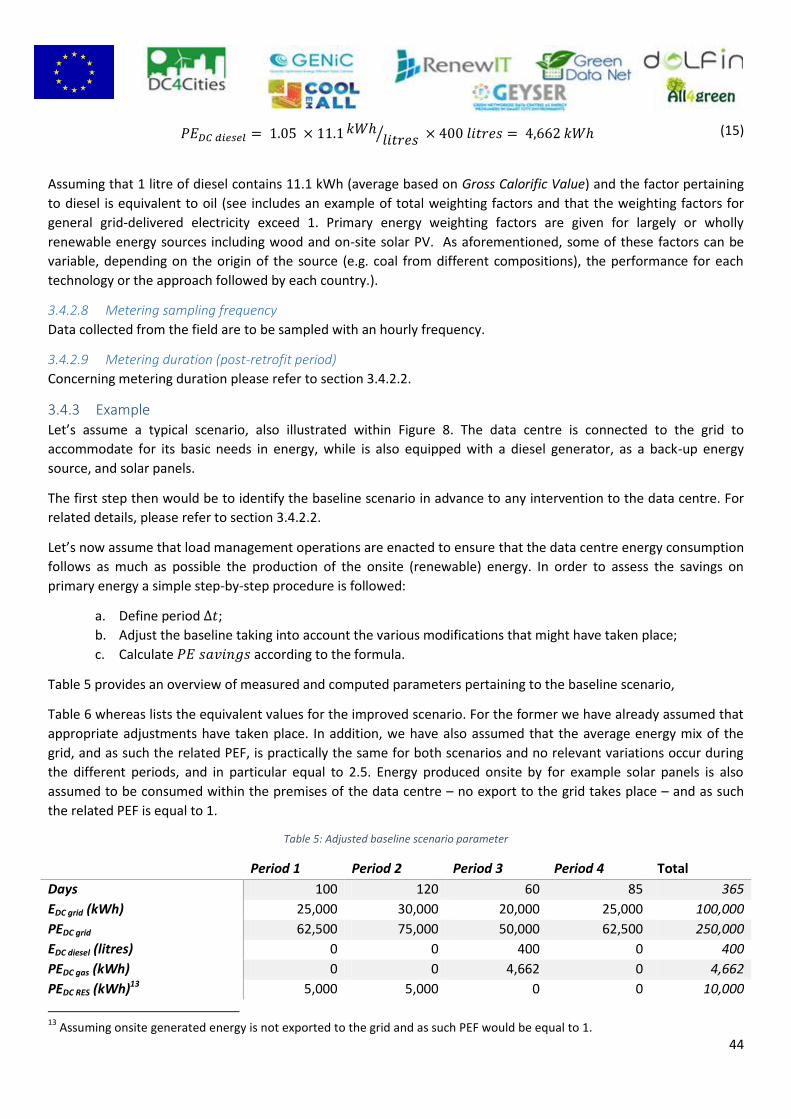
44

(15)

Assuming that 1 litre of diesel contains 11.1 kWh (average based on Gross Calorific Value) and the factor pertaining

to diesel is equivalent to oil (see includes an example of total weighting factors and that the weighting factors for

general grid-delivered electricity exceed 1. Primary energy weighting factors are given for largely or wholly

renewable energy sources including wood and on-site solar PV. As aforementioned, some of these factors can be

variable, depending on the origin of the source (e.g. coal from different compositions), the performance for each

technology or the approach followed by each country.).


Data collected from the field are to be sampled with an hourly frequency.


Concerning metering duration please refer to section 3.4.2.2.

3.4.3 Example Let’s assume a typical scenario, also illustrated within Figure 8. The data centre is connected to the grid to

accommodate for its basic needs in energy, while is also equipped with a diesel generator, as a back-up energy

source, and solar panels.

The first step then would be to identify the baseline scenario in advance to any intervention to the data centre. For

related details, please refer to section 3.4.2.2.

Let’s now assume that load management operations are enacted to ensure that the data centre energy consumption

follows as much as possible the production of the onsite (renewable) energy. In order to assess the savings on

primary energy a simple step-by-step procedure is followed:

a. Define period ;

b. Adjust the baseline taking into account the various modifications that might have taken place;

c. Calculate according to the formula.

Table 5 provides an overview of measured and computed parameters pertaining to the baseline scenario,

Table 6 whereas lists the equivalent values for the improved scenario. For the former we have already assumed that

appropriate adjustments have taken place. In addition, we have also assumed that the average energy mix of the

grid, and as such the related PEF, is practically the same for both scenarios and no relevant variations occur during

the different periods, and in particular equal to 2.5. Energy produced onsite by for example solar panels is also

assumed to be consumed within the premises of the data centre – no export to the grid takes place – and as such

the related PEF is equal to 1.

Table 5: Adjusted baseline scenario parameter

Period 1 Period 2 Period 3 Period 4 Total

Days 100 120 60 85 365

EDC grid (kWh) 25,000 30,000 20,000 25,000 100,000

PEDC grid 62,500 75,000 50,000 62,500 250,000

EDC diesel (litres) 0 0 400 0 400

PEDC gas (kWh) 0 0 4,662 0 4,662

PEDC RES (kWh)13 5,000 5,000 0 0 10,000

13

Assuming onsite generated energy is not exported to the grid and as such PEF would be equal to 1.

45

PEDC (kWh) 67,500 80,000 54,662 62,500 264,662 d.

Table 6: Improved scenario parameters


Days 100 120 60 85 365

EDC grid (kWh) 20,000 25,000 15,000 20,000 80,000

PEDC grid 50,000 62,500 37,500 50,000 200,000

EDC diesel (litres) 0 0 400 0 400

PEDC gas (kWh) 0 0 4662 0 4662

PEDC RES (kWh) 10,000 10,000 5,000 5,000 30,000

PEDC (kWh) 60,000 72,500 47,162 55,000 234,662

In this example, primary energy savings would be equal to 11.34%, even though the total energy consumption in

electricity remains the same.

3.5 CO2 Avoided Emissions

3.5.1 M & V Plan Scope and Metric Overview This section discusses in detail the metric denoting the savings in terms of CO2 emissions generated by a data centre

(CO2Savings), once improvements have taken place with regard to its energetic, economic, or environmental

management.

Naturally, this metric belongs to the same family of metrics as the ones related to the primary energy savings (see

PESavings) and savings on economic expenses (EES). These metrics were initially introduced within the report

released by the cluster as a result of their work on identifying new metrics to accommodate for newly introduced

dimensions such as usage of renewable energy sources, energy re-use, and data centre flexibility mechanism14. The

suggested formula pertaining to the CO2 variant was given as:

(16)

This section, taking as a starting point the above formula, will further elaborate and detail the proposed metric along

with guidelines pertaining to its computation and related measurements.

For all intents and purposes of this section definitions pertaining to commonly used terms are those specified within

ISO/IEC JTC 1/SC39 documents, unless otherwise explicitly stated, and in particular (ISO/IEC JTC 1/SC 39, 2014).

Similarly to PESavings, to better understand what this formula represents, one may collapse the parameters involved

while introducing the percentage aspect as follows:

(17)

14




46

where,

denotes the total CO2 emissions released due to the energy consumed by the data centre during

period , as a summation of discrete intervals15 in time, while

denotes the total CO2 emissions that would have been released due to the energy consumed

by the data centre during the “same” period provided that conditions would have remained the same as in the

baseline scenario, namely no improvements would have taken place.

As in the PESavings, the selected period may depend on the type of the data centre in question, the

characteristics of its business model, the type of the intervention and so forth. Please refer to the section describing

the metric on PESavings for detailed information on this issue.

Obviously for the purposes of this metric we consider only the CO2 emissions released due to the consumption of

energy by the data centre; a full life-cycle analysis of the data centre and its equipment (IT and otherwise), although

important to the environmental sustainability efforts of the sector, is out of scope.

To further elaborate on the computation of this metric, one can decompose its parameters, similarly as in PESavings,

to emissions due to electricity, , and those due to energy consumed in any other form, , such as

for example diesel generator for back-up purposes:

(18)

In particular, emissions related to electricity taken from the grid should be computed as the product of the energy

consumed and the Carbon Emission Factor (CEF) of the site based on regional or national published data for the

selected period.

(19)

As in PESavings, the measurement unit of energy is kWh, while CEF is measured in kgCO2eq/kWh (metric system).

However, in case one wish to use this metric to also evaluate demand response scenarios, where flexibility

mechanisms that involve modifying the energy consumption profile are introduced in the data centre, CEF may not

be considered as a constant value; in this case one may compute this factor for each while taking into account

variations in the (local) electricity mix.

In this case, one should reference the source used for acquiring the appropriate values; Table 7: Recommended

source data for CEF per region. lists recommended sources for obtaining such data, as also presented within (Global

TaskForce, 2014).

Table 7: Recommended source data for CEF per region.

Region Data Source

E.U. http://re.jrc.ec.europa.eu/energyefficiency/covenantofmayors/seap_guidelines_en-2.pdf

http://archive.defra.gov.uk/environment/business/reporting/pdf/100805-guidelines-ghg-conversion-factors.pdf

Japan http://ghg-santeikohyo.env.go.jp/files/calc/itiran.pdf

15

As for PE_savings, discrete interval will depend on the goal pursued to compute the metric, and may vary from a time interval equal to 15 minutes or 1 hour to a time interval of 1 week, month or year.

http://re.jrc.ec.europa.eu/energyefficiency/covenantofmayors/seap_guidelines_en-2.pdf



http://ghg-santeikohyo.env.go.jp/files/calc/itiran.pdf

47

USA http://www.epa.gov/cleanenergy/documents/egridzips/eGRID2007V1_1_year05_SummaryTables.pdf

http://www.energystar.gov/ia/business/evaluate_performance/Emissions_Supporting_Doc.pdf?ac4e-840b

Other sources of energy should also be accounted for; ideally, CO2 emissions data would be gathered from real-time

CO2 meters that collect data from the local power source (natural gas, diesel, fuel oil, coal, turbines/generators/fuel

cells, or other). However, if real-time CO2 emission data is not available, then calculations should be made using the

generator manufacturer(s) data for emission and fuel source, calculated for the specific, actual load profile over time

(The Green Grid, 2010).

In the following we provide information on baseline identification and adjustment, analysis, verification, and

reporting methodology, before presenting a simple example illustrating the proposed methodology.

3.5.2 Measurements


Based on the formula aforementioned and in line with the concept of treating the data centre as a black box the

parameters to be measured are:

Total energy taken by the grid, measured at the meter for each time interval, and consumed during a pre-

selected period of time ; and

Total energy produced and consumed on site for each time interval for immediate and own consumption

(back-up generators, solar panels, and so on), or whenever possible CO2 emissions measurements from real-

time CO2 meters that collect data per local source.

For details on baseline scenario specifications please refer to sections 3.5.2.2 and 3.5.2.3, while for information

related to measurements points to section 3.5.2.4.


See paragraph 3.4 on PESavings metric.




See paragraph 3.4 on PESavings metric in case only energy related measurements are available.

In case one can obtain real time information from CO2 meters dedicated to collect data from a particular source,

then such meters would be located at the output of the source.



In case direct CO2 emissions measurements are possible, meters are necessary to be deployed according to their

manufacturer’s standards and methodology.


See paragraph 3.4 on PESavings.

Similarly, special attention should be paid in case CO2 meters are deployed.



http://www.epa.gov/cleanenergy/documents/egridzips/eGRID2007V1_1_year05_SummaryTables.pdf



48








3.5.3 Example Let’s assume the same scenario as the one described within the document pertaining to the PESavings: A data

centre, located for example in the Netherlands, is connected to the grid to accommodate for its basic needs in

energy, while is also equipped with a diesel generator, as a back-up energy source, and solar panels.


related details, please refer to the PESavings metric.

Let’s now assume that load management operations are put in place to ensure that the data centre energy

consumption follows as much as possible the production of the onsite (renewable) energy. In order to assess the

savings on CO2 emissions the same as in PESavings step-by-step procedure is followed.

Table 8 provides an overview of measured and computed parameters pertaining to the baseline scenario, while

Table 9 lists the equivalent values for the improved scenario. For the former we have already assumed that

appropriate adjustments have taken place.

Table 8: Adjusted baseline scenario calculations.


Days 100 120 60 85 365

E DC grid (KWh) 25,000.00 30,000.00 20,000.00 25,000.00 100,000.00

CO2 DC grid (kgCO2eq) 17,900 21,480 14,320 17,900 71,600

E DC onsite: gen (litres) 0.00 0.00 400.00 0.00 400.00

E DC onsite: gen (kWh) 0.00 0.00 4440.00 0.00 4440.00

CO2 onsite: gen (kgCO2eq) 0.00 0.00 1354.20 0.00 1354.20

E DC onsite: RES (kWh) 5,000.00 5,000.00 0.00 0.00 10,000.00

CO2 onsite: RES (kgCO2eq) 100.00 100.00 0.00 0.00 200.00

Tot. CO2 emissions (kgCO2eq) 18,000.00 21,580.00 15,674.20 17,900.00 73,154.20

Table 9: Improved scenario calculations.


Days 100 120 60 85 365

E DC grid (KWh) 20,000.00 25,000.00 15,000.00 20,000.00 80,000.00

CO2 DC grid (kgCO2eq) 14,320 17,900 10,740 14,320 57,280

E DC onsite: gen (litres) 0.00 0.00 400.00 0.00 400.00

E DC onsite: gen (kWh) 0.00 0.00 4,440.00 0.00 4,440.00

CO2 onsite: gen (kgCO2eq) 0.00 0.00 1,354.20 0.00 1,354.20

E DC onsite: RES (kWh) 10,000.00 10,000.00 5,000.00 5,000.00 30,000.00

49

CO2 onsite: RES (kgCO2eq) 200.00 200.00 100.00 100.00 600.00

Tot. CO2 emissions (kgCO2eq) 14,520.00 18,100.00 12,194.20 14,420.00 59,234.20

Table 10 lists all emissions factors used in the calculations above. So as to keep the example simple, we have

assumed that the emission factor of the grid has remained the same between the baseline year and the one of the

improved scenario.

Table 10: Emissions factors used in example calculations (Source: http://www.eumayors.eu/IMG/pdf/technical_annex_en.pdf)

CEF Value (t CO2 eq / MWh)

grid (NL) 0.716

diesel 0.305

solar panel 0.020

Assuming that 1 litre of diesel contains 11.1 kWh (average based on Gross Calorific Value), consumption of 400 litres

of diesel would be:

(20)

The CO2 emissions savings would then be equal to 19.03 %, even though the total energy consumption in electricity

is essentially the same. The primary energy savings for this example are equal to 11.34 %.

3.6 Economic Saving in Energy Expenses (EES)

3.6.1 M & V Plan Scope and Metric Overview This section is a detailed presentation of the Energy Expenses metric, EES, which provides an expression for overall

economic savings in energy expenses within a data centre, once improvements have taken place with regard to its

energetic, economic, or environmental management.

This metric belongs to the same family of metrics as the ones related to the primary energy savings (see PESavings)

and the CO2 emissions savings (CO2Savings). These metrics were initially introduced within the report released by

the cluster as a result of their work on identifying new metrics to accommodate for newly introduced dimensions

such as usage of renewable energy sources, energy re-use, and data centre flexibility mechanism16. The suggested

formula pertaining to the economic expenses variant was given as:

In general, assuming no changes in contracted power are introduced, no fix costs are included in the analysis (for

example pertaining to grid operators’ fees) or savings due to potentially less related taxes.

The current document, taking as a starting point the above formula, will further elaborate and detail the proposed

metric along with guidelines pertaining to its computation and related measurements.

16


http://www.eumayors.eu/IMG/pdf/technical_annex_en.pdf



50

For all intents and purposes of this document definitions pertaining to commonly used terms are those specified

within ISO/IEC JTC 1/SC39 documents, unless otherwise explicitly stated, and in particular (ISO/IEC JTC 1/SC 39,

2014).

Similarly to PESavings, to better understand what this formula represents, one may collapse the parameters

involved, while introducing the percentage aspect, as follows:

(21)

where:

denotes the total energy consumption of the data centre, pertaining to the grid (electricity, natural gas, and

so on), in kWh during a given time interval as a summation of discrete intervals17 in time;

denotes the average energy cost in €/kWh during the same time interval; it should be noted that the average

cost is calculated by weighting the energy consumptions at different energy prices periods; most commonly such

average cost takes no consideration for costs paid to the energy supplier for power contracted; however, in case of

any modification, fix costs will have to be considered to calculate the energy average cost;

denotes the total energy consumed by the data centre that was produced on site during the same time

interval; and

denotes the average energy cost pertaining to energy produced and consumed on site during the same

time interval. The same approach than for should be followed in case of hourly prices variations.

An effort was made to devise a general metric that takes into account also costs incurred in the set-up of an onsite

energy producing facility. Nevertheless, this metric can be very useful for optimization purposes as well, for example

analysing, once a local source is installed, the potential benefits of using this source during a period (and thus linked

to flexibility mechanisms in data centres). In the case that the simple computation of energy costs is desired, certain

factors may be considered equal to 0, such as terms pertaining to amortization, maintenance, installation and

operational costs, for analysing various scenarios.

The expression current denotes the total cost of the energy consumed by the data centre in its “final” configuration,

measured during time period , while baseline adjusted denotes the total cost of the energy that would have been

consumed by the data centre during the same period, provided that conditions would have remained the same as in

the baseline scenario. Conditions between the two periods will most likely be different, not only in relation to

environmental parameters, but also for IT and facility equipment and workload, especially considering that

continuous optimization efforts may have been put in place. One should, therefore, adjust the baseline by for

example measuring and analysing the correlation of kWh with external parameters, so that these external

parameters can be used to estimate what the consumption would have been during the reporting period.

It is important to remark that revenues coming from exported energy produced onsite will have to be considered to

calculate EES, in case the data centre sells a share of its production (for example photovoltaic surpluses injected to

the electricity grid or recovery heat from a CHP sold to another building).

As already mentioned above, the quantities and , are the results of weighted summations over

period Δt, because energy prices may vary within this period.

17

Discrete interval will depend on the goal pursued to compute the metric, and may vary from a time interval equal to 15 minutes or 1 hour to a time interval of 1 week, month or year.

51

More specifically:

=

(22)

in which the total period is divided in n sub-periods, each with its own energy cost. Similar expressions can be

defined for the other variables.

is provided by the contract between the data centre and the energy supplier. Normally this is a fixed-price

rate, which is agreed upon at the start of the contract. Situations with a variable-price situation must be taken into

account. In this case will be calculated as an average weighted value, thus:

(23)

While represents the electricity as taken from the grid, is computed based on all available sources

of energy within the data centre premises. In a typical scenario where the data centre, for example, has only a

couple of back up diesel generators, the situation is straightforward. One only needs to take into account the

amount of litres or m3 consumed within period multiplied by the (average) cost (€/litre) during the same period,

similarly to the situation above.

However, in case of further energy sources available on site, such as for example PV panels, the total cost pertaining

to energy produced and consumed onsite would be given by the formula below:

(24)

where,

denotes the average cost per unit of energy produced onsite by energy source j.

Depending on the purposes for which the data centre needs to calculate this KPI, energy costs can be

calculated only considering energy costs or also considering other terms, as for example, maintenance costs onsite.

For example, if a data centre wants to evaluate how energy costs will be affected by a demand side management

project, Cost will have to be calculated considering only energy costs.

For other more complex evaluations (as TCO), the inclusion of other terms that take into account investments and

operational costs can be needed. The TCO general expression can be quite complicated. A simplified expression that

can be valid for the purposes of this document is:

(25)

where,

= cost of amortization of equipment/infrastructures in the period Δt

= cost of amortization of installation in the period Δt

= cost of operation (including energy costs) & maintenance in the period Δt

Thus:

(26)

52

3.6.2 Measurements


Based on the formula aforementioned the parameters to be measured are:

Total energy (electricity or other form) consumption taken by the grid and measured at the meter for each

time interval; and

Total primary energy source consumption on site (back-up generators, solar panels, and so on) for each time

interval

For details on baseline scenario specifications please refer to sections 3.6.2.2 and 0, while for information related to

measurements points to section 0.


The baseline is evaluated experimentally measuring energy values at points A, B, POD of the diagram. Given that the

DC can be considered as a “black box”, no other measurements are needed in this case.

To perform the baseline evaluation an appropriate value for Δt must be selected. In principle, we are dealing with an

aggregate value, and therefore Δt corresponds to a relatively long period, typically 1 year.

For practical purposes, in case measurements are bound to a shorter period (e.g. demonstrative project or energy audit to evaluate the feasibility of a project), if it is not possible to carry out the determination of a baseline and current value throughout one year, this can be simulated by assessing the value of the energy consumption in a set of “typical days” and then projecting these on a 1-year period. Although IPMVP does not allow for simulated data, we nevertheless opt for such approach since, at this stage, the idea is to provide a general formula considering expenses savings at data centre level. However, if sub-meters are installed, methodology will be the same as option B (no option A as we are measuring energy). Requisites and characteristics of the set must be determined for the specific data centre under study. Daily values must be collected under different operational conditions of the data centre. This aggregate value can

exhibit significant variations depending on seasonal effects (winter/summer), workload changes (that is working

day/weekend, specific deadlines, and so on) and different hourly prices depending on the day/month.


A need for baseline adjustments arises when some “external factor” introduces a change in the baseline value.

External factors of practical importance are:

• substantial changes in the equipment of the Data centre;

• refurbishment/renovation of the premises where the Data centre is located;

• changes in environmental parameters (temperature, relative humidity, etc.);

• business changes, i. e. partnerships, mergers, acquisitions, opening of new markets/activities;

• significant changes in workloads and/or workload distribution.

Routine adjustments are those that would be done regularly, for example, due to changes in weather conditions or

IT workloads. Most of such external factors introduce non-linear effects in the formulas. For instance, increases in

the total workload of a Datacentre do not imply corresponding proportional increases in the energy consumption. As

an example, the simple adjustment of the baseline through a multiplying factor, therefore a relation obtained as a

linear regression, as in the expression:

Energy consumption = α x independent variable+ b (27)

is hardly ever possible. In general, it is therefore not possible to estimate values for the above parameters “theoretically” (i. e. without performing a new experimental assessment of the baseline). In certain specific cases it

53

might appear possible to perform such an estimate, but a general operational rule cannot be given and the

calculation of the adjustment will have to be performed on a case-by-case basis.

A non-routine adjustment would occur due to an isolated event, for example, an increase of the total DC surface

(new equipment). In this case, a new mathematical model has to be performed. As explained for PEsavings, a new

mathematical model needs to be performed.


Figure 9 Figure 9 illustrates a typical scenario of a data centre. The total energy consumption taken by the grid is

measured at point A, for example with a meter close to the POD. For other forms of energy such as gas, fuel, or

chilled water the measurement is taken at the point of delivery of each source, for example as input to the non-RES

element of Figure 9, while for renewable generation onsite the energy produced and consumed is measured with a

meter at the output of the RES element.

Therefore all forms of energy are considered, as primary (source) energy, and converted in primary energy following

the conversion factors defined in the document pertaining to primary energy savings.

Figure 9: Data Centre Control Volume and Measuring Points


All the required variables can be metered using permanent energy meters. They should be provided of a

communication protocol module such as for example ModbusRTU RS485 or equivalent. The measure error has to be

1% or lower (active energy).


Meter range has to be consistent with the variable range. Meters setup during commissioning should include

consistent unit selection. Meters calibration should take place preferably once a year.

54


Assumptions related to the costs of the electricity and thermal energy in the different countries should be taken into

considerations.


Data collected from the field have to be sampled with an hourly frequency.


Concerning metering duration please refer to section 3.6.2.2.

3.6.3 Example Let us assume a typical scenario, also illustrated within Figure 9. The data centre is connected to the grid to

accommodate for its basic needs in energy, while is also equipped with a diesel generator as a back-up energy

source.


related details, please refer to section 3.6.2.2. After some action has been performed on the data centre, the need

for an assessment of EES arises; a simple step-by-step guide follows:

a. Define period Δt.

b. Calculate the TCO for the onsite energy production plant for the period Δt.

c. Calculate , the cost of a KWh produced onsite

d. Adjust the baseline taking into account the various modifications that might have taken place.

e. Calculate , the average cost of energy provided by an external energy supplier

f. Calculate EES according to the formula.

Table 11 provides an overview of measured and computed parameters pertaining to the baseline scenario, whereas

Table 12 lists the equivalent values for the improved scenario. Let’s assume variable cost of energy per 4 periods

over a total duration of 1 year. For ease of comparison we further assume that energy prices between baseline year

and “current” year remain the same. In addition, we assume that the data centre consumes a total of 100,000 kWh

of energy per year.

Table 11: Adjusted baseline scenario parameter


Days 100 120 60 85 365

EDCgrid (kWh) 25,000 30,000 20,000 25,000 100,000

COSTgrid (€/kWh) 0.2 0.19 0.22 0.21

Tot. Exp. Grid (€) 5,000 5,700 4,400 5,250 20,350

EDCgas (litres) 0 0 400 0 400

Costgas ((€/litres) - - 0.5918 -

Tot. Exp. Onsite (€) - - 234.58 - 234.58

Tot. En. Exp. (€) 5,000 5,700 4,634.58 5,250 20,584.58

Table 12: Improved scenario parameters


18

Dec 2013; http://www.indexmundi.com/commodities/?commodity=diesel&months=120&currency=eur

http://www.indexmundi.com/commodities/?commodity=diesel&months=120&currency=eur

55

Days 100 120 60 85 365

EDCgrid (kWh) 15,000 20,000 15,000 20,000 70,000

COSTgrid (€/kWh) 0.20 0.19 0.22 0.21

Tot. Exp. Grid (€) 3,000 3,800 3,300 4,200 14,207.60

EDCgas (litre) 0 0 400 0 400

EDCRES (kWh) 10,000 10,000 5,000 5,000 30,000

Costgas - - 0.4419 -

CostRES 0.18 0.18 0.18 0.18

Tot. Exp. Onsite (€) 1,800 1,800 1,074.35 900 5,574.35

Tot. En. Exp. (€) 4,800 5,600 4,374.35 5,100 19,874.35

In this example, EES would be equal to 3.45% denoting the percentage of energy related cost savings (even though

the data centre’s total energy consumption remained the same).

3.7 Grid Utilization Factor

3.7.1 M & V Plan Scope and Metric Overview The scope of the M & V plan described hereafter is to provide the specifications required to assess correctly the Grid

Utilization Factor (GUF) belonging to the category: “Renewables integration: Energy produced locally and Renewable

usage. GUF represents the percentage of time that the local generation does not cover the electricity demand (in

this case, a DC, but in general this will be applicable to any kind of consumer), and thus how often energy must be

supplied by the grid..

This metric is linked to the net exported electricity and is defined according to the following formula:

(28)

(29)

where:

is a step function representing the capability of the Renewable Energy Sources (RES) of covering the

demand at time ,

and are the start and end time respectively for GUF monitoring,

represents the net exported electricity at time and is given by:

(30)

where:

is the aggregate exported electricity or the electricity generated at RES,

is the aggregate delivered electricity or the electricity demand.

For the metric calculation purposes equation (31) has to be transformed as follows: 19

Dec 2014; http://www.indexmundi.com/commodities/?commodity=diesel&months=120&currency=eur

http://www.indexmundi.com/commodities/?commodity=diesel&months=120&currency=eur

56

(31)

(32)

Where:

is a step function given by eq. (32),

is the measurement index,

is the number of measurements,

is the average value of the net exported electricity at the sampling period between measurements

and .

3.7.2 Measurements


Following the metric description presented in section 3.7.1, the periods during which the renewable energy

generation is sufficient to cover the electricity demand or not need to be determined. As a result, the following

values have to be assessed:

: the electricity generated at RES and exported to the grid. It can be measured at the point of

connection between the electrical power plant and the grid.

: the electricity acquired from the grid. It can be usually assessed through the electrical counter

installed by the utility for billing reasons.

the portion of time during which the net exported electricity, as given from equation (30) is negative.

The system setup for GUF assessment is depicted in Figure 10. Based on this figure, can be measured at point

B, while can be measured at point C. As a result:

(33)

57

Figure 10: System setup for GUF assessment


The baseyear conditions are the Data Centre (DC) conditions during 12 months preceding the decision to deploy and

use (additional) renewable energy sources. These conditions can be identified from the electricity bill of the utility

serving the DC. Moreover, the following should be taken into account as baseline conditions affecting the DC

electricity consumption:

a report on the number, type and yearly energy profiles of any on-site RES;

a lighting level survey;

a report of the number, type and energy characteristics of IT equipment (CPU, RAM, HDD, networking

devices), along with an estimate of the operating hours and load of each;

a report of the number, type and energy characteristics of non-IT equipment (CRAH, CRAC, etc.), along with

an estimate of the operating hours and load of each;

a report of the number, type and energy characteristics of facility equipment (air-conditioning, heating,

lighting, etc.), along with an estimate of the operating hours and load of each;

a record of the temperature setting of cooling equipment;

a record of the used capacity of CPUs, RAMs, HDDs;

a record of the IT load for each month of the year;

a record of the provided services, along with the contracted SLAs and a count on the number of customers

a report of the number, type and energy characteristics of energy-reuse devices;

a record of the number of working days and hours for each month of the year;

a summary of weather and climatic data for each month of the year;

a report on the number, type, position and error of metering devices;

a record of any energy-efficient techniques in place;

the goal of workload and energy optimization (if any) per day for each month of the year.

The sampling period for measurements should be at least 15 minutes.

The baseyear energy use is metered at point C of Figure 10 spanning a 12-month period.

The baseyear renewable energy use is metered at point B of Figure 10 spanning a 12-month period.

58

The baseyear energy data shall be analysed as follows. Linear regression shall be applied on monthly total and

renewable electricity use, as well as total electricity demand, metering period length and degree days. The latter

shall be derived by third party information providers. Correlation of weather with electricity demand, (total or

renewable) supply and (total or renewable) use is expected to be identified.

Savings derived from renewable energy usage will be determined under post-retrofit conditions.

3.7.2.2.1 Baseyear Electricity Use

The baseyear electricity use for Eq. (32) is taken directly from the metering equipment at point C Figure 10 without

adjustment.

3.7.2.2.2 Baseyear Renewable Energy Use

The baseyear renewable energy use for Eq. (30) is taken directly from the metering equipment at point B of Figure

10 without adjustment.

3.7.2.2.3 Post-Retrofit Electricity Use

The post-retrofit electricity use for Eq. (30) is taken from the metering equipment at point C of Figure 10 without

adjustment.

3.7.2.2.4 Post-Retrofit Renewable Energy Use

The post-retrofit renewable energy use for Eq. (30) is taken from the metering equipment at point B of Figure 10

without adjustment.


Baseline adjustments may be needed to bring baseyear energy use to the conditions of the post-retrofit period.

Adjustments are not needed to calculate the KPI, but to compare the KPI between two different time intervals (e.g.

two consecutive years after installing a PV power plant in the DC).

3.7.2.3.1 Routine Adjustments

3.7.2.3.1.1 Electricity Demand

The electricity demand is expected to be affected by changes in the external temperature (Degree Days) and the

number of operating days. As result, the following routine adjustments are needed:

The electricity demand of the cooling equipment may vary depending on the ambient temperature.

Appropriate adjustments should be made, based on manufacturer’s specifications.

The electricity demand of air-conditioning and heating facilities should be adjusted to ambient temperature

based on manufacturers’ specifications.

Electricity demand due to lighting requirements within the DC may vary depending on the daylight hours.

Electricity demand may vary due different IT workload between years and appropriate adjustments should

be made

3.7.2.3.1.2 Renewable Energy Generation

The electricity generation of installed on-site RES may be affected by weather conditions, such as solar radiation and

wind speed. Specifically, solar radiation directly influences the production of photovoltaic (PV) and solar thermal

systems, while the wind speed directly influences the production of wind turbines. Adjustments on the renewable

energy generation must be made according to the manufacturers’ datasheet for the current configuration and

weather conditions.

59

3.7.2.3.2 Non-routine Adjustments

Procurement of new equipment during the post retrofit period raises the need for non-routine adjustments. The

new equipment may refer to IT (CPU, RAM, HDD, networking devices), non-IT (cooling equipment), facilities (air-

conditioning units, heating, lighting), as well as on-site RES. IT and non-IT installed power affects the amount of

electricity demand and consumption. Moreover, software changes, such as cloud adoption or virtualization may

affect the electricity demand of the IT equipment. The adjustments should refer to both the electricity consumption

and demand, referring to manufacturers’ factsheets on electricity consumption.

In the following an example is given for local RES, which affect the amount of exported electricity. The impact on the

annual balance depends on the typology of renewable energy source that has been installed. The adjustment factor

depends on the ratio between annual production and installed power. In other words:

(34)

Where:

: baseline exported energy adjusted according to normalization variables for the RES ,

: installed peak power for the RES during the test period,

: installed peak power for the RES during the baseline period,

: specific energy factor (kwh/kWp) for the RES


The area of interest for GUF measurements is depicted in Figure 10 within a grey-line polygon.

Maximum boundaries: energy balance between electricity exported to the grid and electricity delivered to the grid is

measured at the POD. All onsite renewable power plants are connected below the POD. In this case a single

metering point is needed.

Minimum boundaries: each single onsite renewable energy sources power plant is metered and each single power

supply switchboard is metered too.




- Meters range has to be consistent with the metered variables range and these meters should allow a


- Meters have to be provided of a communication module (ModbusRTU RS485 protocol or equivalent),have to


database. A properly sized storage system has to be designed and installed and data must be available for

the next phase of analysis and verification. In this way, each meter, becomes a node of the network.

- Meters have to be equipped with the required auxiliary devices such as amperometric transformers,

voltmetric commutators, surge protectors and surge arresters

- Meters and auxiliary devices have to be chosen according to the supply voltage. LV point of measures have

to be preferred on MV point of measures due to lower metering costs.


networking have to be compliant with the existing standards (ANSI, IEC, IEEE, CEI EN). The requirements specified in

these standards have to be considered as minimum values for the meters under normal working conditions. For

60

special application, higher constraints might be necessary and should be agreed between the user and the

manufacturer.






Once the measurement system is installed it a test procedure has to be applied. During this procedure, once the

meter settings are set, the measure collected by the installed meter is compared to the measure collected trough a

portable configured meter. The test procedure must not be confused with the calibration procedure performed by


the sampling time.


Every time the gateway don’t communicate with the storage system or one or more nodes don’t communicate with

the gateway it is necessary to check and solve the problems in due time.

Periodically (once a year) it is important to inspect the measurement equipment and repeat the calibration

procedure.

Every time hardware changes occur, the compliance between the meter range and the physical variable range must

be checked and guaranteed.


No comment


The required meter sampling frequency is 64 samples/cycle. The metered energy minimum sampling frequency is of

one second. Higher sampling rates are not required since the variability of the metered physical values is not so

rapid. GUF value must be stored at least every 15 minutes.


Concerning metering duration at least a whole year data set should be collected: this is because renewables have a

yearly production profile.

3.8 Analysis & Verification

Important Notice: The whole section is going to be the same for all identified metrics, namely it should be

consistent across all developed methodologies. General ways of dealing with analysis and verification will be

provided, their application depending on DC configurations.

3.8.1 Error Filtering Erroneous measurements introduce inaccuracies to the measured quantities, which subsequently propagate to the

calculation of the metrics. As a result, the performance indicators are distorted, providing a falsified picture of the

system performance. Therefore, error filtering techniques must be employed, in order to mitigate the effect of

erroneous measurements on the calculation of the KPIs.

61

In the direction of pinpointing measurements that are likely to be erroneous the mean value and the standard

deviation of the last 5 measurements are retained and compared to the value of the current measurement. Having a

sample of actual readings

the Mean value of the measurements is defined by

,

(35)

and the Sample Standard Deviation is defined by

(36)

Thus, if the current measurement falls within the range , it can be considered to be within

the expected range. However, if the measurement falls out of this range, the measurement is flagged as potentially

erroneous and the DC operator is prompted to repeat the measurement. If the repetition provides a very similar

value (for example, within 2% of the value flagged as potentially erroneous), then the flag is eliminated and the value

is accepted as correct. The new measurement is then registered and used for the calculation of the metric. Else, if

the values are very different, it is flagged as erroneous.

Apart from employing the above process for pinpointing potentially erroneous measurements, the DC operator also

has to isolate erroneous measurements. In particular, measurements that, given the specifics of each DC, are clearly

out of range and remain out of range despite the repetition of the measurement should be filtered out by the DC

operator. The erroneous measurements are then substituted by the average of the preceding ( ) and the

following ( measurement.

3.8.2 Statistical Analysis of Baseline models The statistical analysis and evaluation of the baseline models is only applicable to metrics where baseline

adjustments are required. Such statistical analyses are essential to evaluate the accuracy of the baseline models.

Specifically, in order to evaluate the extent to which the variations of the actual baseline data are explained by the

baseline model the Coefficient of Determination ( ) should be calculated. is defined by

, (37)

where:

is the model predicted value at the individual time period

is the actual observed value at the individual time period

is the mean value of the actual observed values, as defined by eq. (35)

The range of the possible values of the coefficient of determination is 0 to 1. A value of zero indicates a poor

baseline model where the variations of the actual values are not explained by the model and a value of 1 indicates

an excellent baseline model predicting the variations of the actual observed values to the fullest. In general, the

closest the value of the coefficient of determination is to 1 the better the baseline model is. A generally accepted

value of is 0.75, whereas low values of indicate that the baseline model needs to be improved.

3.8.3 Uncertainty analysis of the results achieved In order to evaluate the achieved results (primarily through the calculation of the saving KPIs) we need to validate

their accuracy and precision. In this course, the standard error of the reported results needs to be defined along with

the expected range of the results with a given confidence level.

62

In general, if a quantity is involved in the calculation of the achieved results, we can obtain the standard deviation of

the measured quantity by eq. (36). However, if not just a sample, but the entire population of measurements of the

measured quantity is available, then the population standard deviation is defined by

, (38)

and the Standard Error is defined by

SE =

,

(39)

However, if a baseline adjusted quantity is involved in the calculation of the achieved result the standard error of the

baseline adjusted quantity is defined by

, (40)

where, is the (baseline) model predicted value at the individual time period , is the actual observed value at

the individual time period and is the number of independent variables in the baseline model.

Moreover, if the achieved result is obtained as the sum or difference of independent quantities of

given standard error (SE) the standard error of the result can be estimated by

, (41)

Having defined the standard error, one can define the absolute precision at a given confidence level and the

estimated range of the result with the predefined confidence level.

To elaborate, the Absolute Precision is defined as: t · SE, where t depends on the number of actual readings n and is

obtained from sample standard error tables (Table 13). Such t-Tables can be found in statistic tables and books20.

Table 13: t-Table

Degrees of

Freedom (DF)

Confidence Level Degrees of

Freedom (DF)

Confidence Level

95% 90% 80% 50% 95% 90% 80% 50%

1 12.71 6.31 3.08 1.00 16 2.12 1.75 1.34 0.69

2 4.30 2.92 1.89 0.82 17 2.11 1.74 1.33 0.69

3 3.18 2.35 1.64 0.76 18 2.10 1.73 1.33 0.69

4 2.78 2.13 1.53 0.74 19 2.09 1.73 1.33 0.69

5 2.57 2.02 1.48 0.73 21 2.08 1.72 1.32 0.69

20

http://www.evo-world.org/index.php?option=com_rsform&formId=125&lang=en

63

6 2.45 1.94 1.44 0.72 23 2.07 1.71 1.32 0.69

7 2.36 1.89 1.41 0.71 25 2.06 1.71 1.32 0.68

8 2.31 1.86 1.40 0.71 27 2.05 1.70 1.31 0.68

9 2.26 1.83 1.38 0.70 31 2.04 1.70 1.31 0.68

10 2.23 1.81 1.37 0.70 35 2.03 1.69 1.31 0.68

11 2.20 1.80 1.36 0.70 41 2.02 1.68 1.30 0.68

12 2.18 1.78 1.36 0.70 49 2.01 1.68 1.30 0.68

13 2.16 1.77 1.35 0.69 60 2.00 1.67 1.30 0.68

14 2.14 1.76 1.35 0.69 120 1.98 1.66 1.29 0.68

15 2.13 1.75 1.34 0.69 ∞ 1.96 1.64 1.28 0.67

DF = n-1

Where n = sample size.

Subsequently, the true value of any statistical estimate is expected with a given confidence level, to fall with the

range defined by

Range = estimate ± absolute precision (42)

Where “estimate” is any statistically derived value of a parameter of interest and in the context of the above analysis

the value of the achieved result (primarily savings result).

Thus, the average value of a set of 6 measurements

Measurement Actual Reading

1 15

2 18

3 13

4 19

5 18

6 17

is defined by the Mean value of the measurements

(43)

the Variance

64

(44)

the Standard Error

SE =

(45)

And for a confidence level of 95% the absolute precision

t · SE = 2.57 · 0.919=2.36 (46)

So there is a 95% confidence that the true mean value lies in the range

Range = 16.7 ± 2.36. (47)

3.9 Reporting

3.9.1 Reporting format An indicative reporting template is presented hereafter.

Metering Equipment:

Metering Point:

Metering Sampling Frequency:

Metering Assumptions:

Date / Time Measurable Variable 1

Value:

5 Last Measurements Measurable Variable 2

Value:

5 Last Measurements

Mean Deviation Mean Deviation

3.9.2 Reporting frequency The frequency of such a report is determined by the metering duration defined in Paragraph X.2.9 of each metric.

65

4 References

ASHRAE. (2009). Real-Time Energy Consumption Measurements in data centers . American Society of Heating,

Refrigerating and Air-Conditioning Engineers, Inc. . Atlanta, GA, USA: ASHRAE.

EIA. (2010). Energy Calculators. White Paper, EIA.

Global TaskForce. (2014). Harmonizing Global Metrics for Data Center Energy Efficiency.

ISO/IEC JTC 1/SC 39 ITEE. (2015). ISO/IEC CD 30134-4: Information Technology -- Data Centres -- Key performance

indicators -- Part 4: IT Equipment Energy Efficiency for Servers (ITEE).

ISO/IEC JTC 1/SC 39 PUE. (2015). ISO/IEC DIS 30134-2: Information Technology -- Data Centres -- Key performance

indicators -- Part 2: Power usage effectiveness (PUE).

ISO/IEC JTC 1/SC 39 REF. (2015). ISO/IEC DIS 30134-3: Information Technology -- Data Centres -- Key Performance

Indicators -- Part 3: Renewable Energy Factor (REF).

The Green Grid / ASHRAE. (2013). PUE : A Comprehensive Examination of the Metric.

The Green Grid. (2010). ERE: A Metric for Measuring the Benefit of Reuse Energy from a Data Center. The Green Grid.

The Green Grid.

The Green Grid. (n.d.). Usage and Public Reporting Guidelines for The Green Grid's Infrastructure Metrics PUE/DCiE.

Global TaskForce. (2014). Harmonizing Global Metrics for Data Center Energy Efficiency.

ISO/IEC JTC 1/SC 39. (2014). ISO/IEC DIS 30134-2: Information Technology -- Data Centres -- Key performance

indicators -- Part 2: Power usage effectiveness (PUE).

Molebroek, E., Stricker, E., & Boermans, T. (2011). Primary Energy Factors for electricity in buildings. Ecofys

Netherlands B.V.

The Green Grid. (2010). Carbon Usage Effectiveness (CUE): A Green Grid Data Center Sustainability Metric.

Noris, F., Musall, E., Salom, J., Berggren, B., Jensen, S. Ø., Lindberg, K., & Sartori, I. (2014). Implications of weighting

factors on technology preference in net zero energy buildings. Energy and Buildings, 82, 250-262.

smart city cluster collaboration, task 4. measurement and verification methodology for energy,...

Technology

dc4citiesenea metric

amsterdam review

metric description

metric mv synopsis metric

review figures

jaume salom renewitirec

partners artemis voulkidis

data centre integration