smart antennas at handsets for the 3g wideband cdma ... antennas at handsets for the 3g wideband...
TRANSCRIPT
Smart Antennas at Handsets for the 3G Wideband CDMA Systems and
Adaptive Low-Power Rake Combining Schemes
Suk Won Kim
Dissertation submitted to the Faculty of the
Virginia Polytechnic Institute and State University
in partial fulfillment of the requirements for the degree of
Doctor of Philosophy
in
Computer Engineering
Dong S. Ha, Chair
James R. Armstrong
F. Gail Gray
Scott F. Midkiff
Jeffrey H. Reed
July 2, 2002
Blacksburg, Virginia
Key Words: Smart Antennas, Low-Power Design, Adaptive Rake Combiner, Hybrid Combining
Copyright 2002, Suk Won Kim
Smart Antennas at Handsets for the 3G Wideband CDMA Systems and
Adaptive Low-Power Rake Combining Schemes
Suk Won Kim
ABSTRACT
Smart antenna technology is a promising means to overcome signal impairments in
wireless personal communications. When spatial signal processing achieved through smart
antennas is combined with temporal signal processing, the space-time processing can mitigate
interference and multipath to yield higher network capacity, coverage, and quality.
In this dissertation, we propose a dual smart antenna system incorporated into handsets for
the third generation wireless personal communication systems in which the two antennas are
separated by a quarter wavelength (3.5 cm). We examine the effectiveness of a dual smart
antenna system with diversity and adaptive combining schemes and propose a new combining
scheme called hybrid combining. The proposed hybrid combiner combines diversity combiner
and adaptive combiner outputs using maximal ratio combining (MRC). Since these diversity
combining and adaptive combining schemes exhibit somewhat opposite and complementary
characteristics, the proposed hybrid combining scheme aims to exploit the advantages of the two
schemes.
To model dual antenna signals, we consider three channel models: loosely correlated fading
channel model (LCFCM), spatially correlated fading channel model (SCFCM), and envelope
correlated fading channel model (ECFCM). Each antenna signal is assumed to have independent
Rayleigh fading in the LCFCM. In the SCFCM, each antenna signal is subject to the same
Rayleigh fading, but is different in the phase due to a non-zero angle of arrival (AOA). The
LCFCM and the SCFCM are useful to evaluate the upper and the lower bounds of the system
performance. To model the actual channel of dual antenna signals lying in between these two
channel models, the ECFCM is considered. In this model, two Rayleigh fading antenna signals
for each multipath are assumed to have an envelope correlation and a phase difference due to a
non-zero AOA. To obtain the channel profile, we adopted not only the geometrically based

single bounce (GBSB) circular and elliptical models, but also the International
Telecommunication Union (ITU) channel model.
In this dissertation, we also propose a new generalized selection combining (GSC) method
called minimum selection GSC (MS-GSC) and an adaptive rake combining scheme to reduce the
power consumption of mobile rake receivers. The proposed MS-GSC selects a minimum number
of branches as long as the combined SNR is maintained larger than a given threshold. The
proposed adaptive rake combining scheme which dynamically determines the threshold values is
applicable to the three GSC methods: the absolute threshold GSC, the normalized threshold GSC,
and the proposed MS-GSC. Through simulation, we estimated the effectiveness of the proposed
scheme for a mobile rake receiver for a wideband CDMA system. We also suggest a new power
control strategy to maximize the benefit of the proposed adaptive scheme.

iv
Dedication
This dissertation is dedicated to my wife, Eun Hee, my daughters, Min Joo and Amy Gina,
and my son, Brian Sanghyun, for all their love and support.

v
Acknowledgments
First above all, I would like to thank God for his grace and love. I would like to express my
gratitude and appreciation to my advisor, Dr. Dong S. Ha, for his guidance and support
throughout my graduate career at Virginia Tech. His suggestions and advice allowed me to
overcome the difficult times during my research. I also would like to thank Dr. James R.
Armstrong, Dr. F. Gail Gray, Dr. Scott F. Midkiff, and Dr. Jeffrey H. Reed for serving on the
advisory committee. My special thanks go to Dr. Reed and Dr. Jeong Ho Kim for their helpful
and insightful comments and encouragements.
I would like to give thanks to Samsung Electronic Co., Ltd. for awarding me a scholarship
to pursue the Ph. D. degree. Special thanks are directed to people in Samsung Electronic Co.,
Ltd., Dr. Kwang Hyun Kim, Dr. Yun Tae Lee, and Mr. Ja Man Koo, for their encouragements
and supports.
Byung-Ki Kim, Kyung Kyoon Bae, and SeongYoup Suh deserve thanks for their helpful
discussions about the dissertation. I am also thankful to the group members: Han Bin Kim, Jia
Fei, Carrie Aust, Meenatchi Jagasivamani, Steve Richmond, Nate August, Jos Sulistyo, Hyung-
Jin Lee, Jina Kim, Chad Pelino, WooCheol Chung, Kyehun Lee, and Sookyoung Kim. I have
spent a lot of good time with my friends and their family: Dong-Jin Lee, Jae Young Choi,
Byeong-Mun Song, Tae-In Hyon, Jae-Hong Park, Jahng Sun Park, Jun Hyung Kim, Chang-Hyun
Jang, and Hwandon Jun. I have also spent lots of valuable time with the church members and
their family: Jeong-Hoi Koo, Gwi Bo Byun, Junghwa Cho, Sang Eon Chun, Seung Yo Lee, and
Mun Ki Lee.
Finally, I would like to give my appreciations to my family: my wife, Eun Hee Lee, my
children, Min Joo, Amy Gina, and Brian Sanghyun, my parents, Sung Ho Kim and Kyu Ja Kim,
and my parents-in-law, Jang Suk Lee and Myo Soon Kim.
vi
Table of Contents
Chapter 1 Introduction .................................................................................................................... 1
Chapter 2 Preliminaries................................................................................................................... 6
2.1 Smart Antennas...................................................................................................................... 6
2.1.1 Introduction to Smart Antennas ....................................................................................... 6
2.1.2 Smart Antenna Algorithms ............................................................................................ 10
2.1.3 Smart Antennas at Handsets .......................................................................................... 13
2.2 Third Generation Wireless Personal Communication Systems ........................................... 17
2.2.1 The 3GPP System .......................................................................................................... 18
2.2.2 The cdma2000 System................................................................................................... 20
2.3 Channel Model..................................................................................................................... 21
2.3.1 GBSB Model.................................................................................................................. 23
2.3.2 ITU Channel Model ...................................................................................................... 25
2.4 Low-Power VLSI Design .................................................................................................... 26
2.5 Generalized Selection Combining ....................................................................................... 28
2.6 Monte Carlo Simulation....................................................................................................... 31
2.7 Summary...............................................................................................................................32
Chapter 3 Smart Antennas at Handsets and Adaptive Rake Combining Scheme ........................ 33
3.1 Smart Antennas at Handsets ................................................................................................ 33
3.1.1 Diversity Combining...................................................................................................... 33
3.1.2 Adaptive Combining...................................................................................................... 35
3.1.3 Hybrid Combining ......................................................................................................... 36
3.2 Channel Model..................................................................................................................... 37
3.2.1 Loosely and Spatially Correlated Fading Channel Models ........................................... 38
3.2.2 Envelope Correlated Fading Channel Model................................................................. 40
3.2.3 Procedure to Obtain Channel Profile using the GBSB Models ..................................... 42
3.2.4 Channel Model Including the Lognormal Fading.......................................................... 44
vii
3.3 Low-Power Rake Receiver Design...................................................................................... 45
3.3.1 Minimum Selection GSC............................................................................................... 45
3.3.2 Adaptive Rake Combining Scheme............................................................................... 48
3.3.3 Power Control Strategy.................................................................................................. 54
3.4 Summary...............................................................................................................................54
Chapter 4 Performance of Smart Antennas at Handsets............................................................... 55
4.1 Performance of Diversity Combining for the 3GPP System ............................................... 55
4.1.1 Simulation Environment ................................................................................................ 55
4.1.2 Simulation Results under the GBSB Circular Model .................................................... 56
4.1.3 Simulation Results under the GBSB Elliptical Model................................................... 63
4.2 Performance of Adaptive Combining for the 3GPP System ............................................... 70
4.2.1 Simulation Environment ................................................................................................ 70
4.2.2 Simulation Results for the AC ....................................................................................... 71
4.3 Performance of Hybrid Combining for the 3GPP System................................................... 74
4.3.1 Simulation Environment for the GBSB Models ............................................................ 74
4.3.2 Performances of the DC and the AC for the GBSB Models.......................................... 75
4.3.3 Performance of the HC for the GBSB Models .............................................................. 80
4.3.4 Simulation Environment for the ITU Channel Model ................................................... 82
4.3.5 Performance of the DC, the AC, and the HC for the ITU Channel Model.................... 83
4.4 Performance of Diversity Combining for the cdma2000 System ....................................... 88
4.4.1 Simulation Environment ................................................................................................ 88
4.4.2 Simulation Results ......................................................................................................... 89
4.5 Performance of Adaptive Combining for the cdma2000 System ........................................ 91
4.5.1 Simulation Environment ................................................................................................ 91
4.5.2 Simulation Results ......................................................................................................... 93
4.6 Summary...............................................................................................................................95
Chapter 5 Performance of MS-GSC and Adaptive Rake Combining Scheme............................. 96
5.1 Simulation Environment ...................................................................................................... 96
5.2 Performance of GSCs: GSC, MS-GSC, AT-GSC, and NT-GSC........................................ 97

viii
5.3 Performance of Adaptive Rake Combiners ....................................................................... 101
5.4 Summary.............................................................................................................................107
Chapter 6 Conclusion.................................................................................................................. 108
References................................................................................................................................... 110
Appendix A: Simulation Model for the 3GPP WCDMA System .............................................. 117
A.1 Matlab Codes for the Hybrid Combiner ........................................................................... 117
A.1.1 System and Model Parameters.................................................................................... 117
A.1.2 Simulation Core .......................................................................................................... 120
A.1.3 Post Processing ........................................................................................................... 125
A.2 Matlab Codes for the MS-GSC and the Adaptive Combining Scheme............................ 127
A.2.2 System and Model Parameters................................................................................... 127
A.2.2 Simulation Core .......................................................................................................... 131
A.2.3 Post Processing ........................................................................................................... 137
Vita.............................................................................................................................................. 139
ix
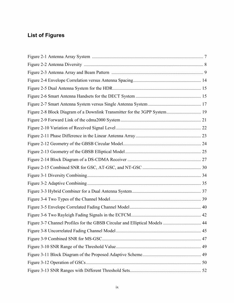
List of Figures
Figure 2-1 Antenna Array System ................................................................................................. 7
Figure 2-2 Antenna Diversity ........................................................................................................ 8
Figure 2-3 Antenna Array and Beam Pattern ................................................................................ 9
Figure 2-4 Envelope Correlation versus Antenna Spacing........................................................... 14
Figure 2-5 Dual Antenna System for the HDR............................................................................. 15
Figure 2-6 Smart Antenna Handsets for the DECT System ......................................................... 15
Figure 2-7 Smart Antenna System versus Single Antenna System .............................................. 17
Figure 2-8 Block Diagram of a Downlink Transmitter for the 3GPP System.............................. 19
Figure 2-9 Forward Link of the cdma2000 System...................................................................... 21
Figure 2-10 Variation of Received Signal Level .......................................................................... 22
Figure 2-11 Phase Difference in the Linear Antenna Array......................................................... 23
Figure 2-12 Geometry of the GBSB Circular Model.................................................................... 24
Figure 2-13 Geometry of the GBSB Elliptical Model .................................................................. 25
Figure 2-14 Block Diagram of a DS-CDMA Receiver ................................................................ 27
Figure 2-15 Combined SNR for GSC, AT-GSC, and NT-GSC ................................................... 30
Figure 3-1 Diversity Combining................................................................................................... 34
Figure 3-2 Adaptive Combining ................................................................................................... 35
Figure 3-3 Hybrid Combiner for a Dual Antenna System............................................................ 37
Figure 3-4 Two Types of the Channel Model............................................................................... 39
Figure 3-5 Envelope Correlated Fading Channel Model.............................................................. 40
Figure 3-6 Two Rayleigh Fading Signals in the ECFCM............................................................. 42
Figure 3-7 Channel Profiles for the GBSB Circular and Elliptical Models ................................. 44
Figure 3-8 Uncorrelated Fading Channel Model .......................................................................... 45
Figure 3-9 Combined SNR for MS-GSC...................................................................................... 47
Figure 3-10 SNR Range of the Threshold Value.......................................................................... 49
Figure 3-11 Block Diagram of the Proposed Adaptive Scheme................................................... 49
Figure 3-12 Operation of GSCs .................................................................................................... 50
Figure 3-13 SNR Ranges with Different Threshold Sets.............................................................. 52

x
Figure 4-1 Dual Smart Antenna Receiver with Diversity Combiner............................................ 56
Figure 4-2 BERs with Three Diversity Combining Schemes and Two Channel Models ............ 59
Figure 4-3 BERs with Various Antenna Distances....................................................................... 60
Figure 4-4 BERs with Various Maximum Delays........................................................................ 61
Figure 4-5 BERs with Various Numbers of Users........................................................................ 62
Figure 4-6 BERs with Various Numbers of Multipaths ............................................................... 63
Figure 4-7 BERs with Three Diversity Combining Schemes and Two Channel Models ............ 65
Figure 4-8 BERs with Various Numbers of Users........................................................................ 66
Figure 4-9 BERs with Various Mobile Velocities........................................................................ 67
Figure 4-10 BERs with Various Numbers of Multipaths ............................................................. 68
Figure 4-11 BER Comparison for the GBSB Circular and Elliptical Models.............................. 69
Figure 4-12 BERs with the GBSB Elliptical and Circular Models .............................................. 72
Figure 4-13 BERs with Various Mobile Velocities...................................................................... 73
Figure 4-14 Performance of the DC and the AC with Various Antenna Distances ..................... 76
Figure 4-15 Performance of the DC and the AC with Various Mobile Velocities....................... 77
Figure 4-16 Performance of the DC and the AC with Various Envelope Correlations................ 79
Figure 4-17 Performance of the HC with Various Mobile Velocities .......................................... 82
Figure 4-18 Performance of the DC, the AC, and the HC............................................................ 85
Figure 4-19 Performance of the HC with Various Antenna Distances......................................... 86
Figure 4-20 Performance of the DC and the AC with Various Mobile Velocities....................... 87
Figure 4-21 Building Blocks of an Adaptive Rake Receiver for Smart Antennas ....................... 92
Figure 5-1 BER Performance with Pedestrian B Channel............................................................ 98
Figure 5-2 BER Performance with Vehicular A Channel .......................................................... 100
Figure A-1 System and Model Parameters for the HC............................................................... 120
Figure A-2 Simulation Core for the HC ......................................................................................125
Figure A-3 Post Processing for the HC....................................................................................... 126
Figure A-4 System and Model Parameters for the GSCs ........................................................... 131
Figure A-5 Simulation Core for the GSCs.................................................................................. 136
Figure A-6 Post Processing for the GSCs................................................................................... 138
xi
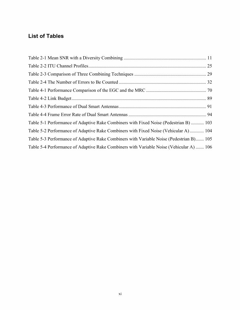
List of Tables
Table 2-1 Mean SNR with a Diversity Combining ...................................................................... 11
Table 2-2 ITU Channel Profiles.................................................................................................... 25
Table 2-3 Comparison of Three Combining Techniques ............................................................. 29
Table 2-4 The Number of Errors to Be Counted .......................................................................... 32
Table 4-1 Performance Comparison of the EGC and the MRC ................................................... 70
Table 4-2 Link Budget .................................................................................................................. 89
Table 4-3 Performance of Dual Smart Antennas.......................................................................... 91
Table 4-4 Frame Error Rate of Dual Smart Antennas .................................................................. 94
Table 5-1 Performance of Adaptive Rake Combiners with Fixed Noise (Pedestrian B) ........... 103
Table 5-2 Performance of Adaptive Rake Combiners with Fixed Noise (Vehicular A) ............ 104
Table 5-3 Performance of Adaptive Rake Combiners with Variable Noise (Pedestrian B)....... 105
Table 5-4 Performance of Adaptive Rake Combiners with Variable Noise (Vehicular A) ....... 106
1
Chapter 1 Introduction
A smart antenna is an antenna array (or multiple antennas) that can adapt to the
environment in which it operates [1]. Smart antenna technology has been used to overcome
signal impairments in wireless personal communications. When spatial signal processing
achieved through a smart antenna is combined with temporal signal processing, the space-time
processing can mitigate propagation distortion and interference to enable higher network
capacity, coverage, and quality [2]-[9]. A smart antenna not only suppresses interference, but
also combats multipath fading by combining multiple antenna signals.
To process multiple antenna signals, two combining schemes—diversity combining and
adaptive combining—can be employed. Diversity combining exploits the spatial diversity among
multiple antenna signals and achieves higher performance. There are four classical diversity
combining schemes: switched diversity, selection diversity, equal gain combining, and maximal
ratio combining (MRC) [10]. After weighting each antenna signal proportional to its signal to
noise ratio (SNR), MRC combines each signal, thus providing maximum output SNR. Adaptive
combining is based on dynamic reconfiguration in that the antenna weights are dynamically
adjusted to enhance the desired signal while suppressing interference signals to maximize signal
to interference plus noise ratio (SINR). It achieves the same performance as the MRC without
presence of interference. The performance of adaptive combining is sometimes limited under
certain circumstances, such as when the angular separation between desired signal and
interference is small or the noise level is high [9].
Because of concerns with high system complexity and high power consumption, smart
antenna techniques have been considered primarily for base stations so far [11]-[18]. A common
belief is that closely spaced antennas are ineffective for exploiting diversity. However, recent
2
measurement results indicate that even closely spaced antennas (such as 0.15 wavelength)
provide a low envelope correlation to yield a diversity gain [19].
Recently, smart antenna techniques have been applied to mobile terminals [20]-[23]. For
example, the high data rate (HDR) system (adopted as IS-856 and also known as 1xEV DO)
developed by Qualcomm employs dual antennas at a mobile station [20]. A dual antenna system
for handsets was also investigated for the digital European cordless telephone (DECT) system
for the indoor radio channel [21]. Also, one of the third generation wireless personal
communication systems, third generation partnership project (3GPP) [24],[25], requires antenna
diversity at base stations and optionally at mobile stations [26]. Antenna diversity is also applied
to the IEEE 802.11 wireless local area network (WLAN) system [27]. Due to the compact size
and stringent cost of handsets and the limited battery capacity, smart antennas at handsets should
have low circuit complexity and low power dissipation. To justify employment of smart antennas
at handsets, the performance gain should be large enough to offset the additional cost and power
consumption.
In this dissertation, we propose a dual smart antenna system incorporated into handsets for
the third generation (3G) wireless personal communication systems in which the two antennas
are separated by a quarter wavelength (3.5 cm) [28]-[32]. We present the effectiveness of a dual
smart antenna system and propose a new combining scheme called a hybrid combiner (HC) [31].
A diversity combiner (DC) combines two rake receiver outputs using a diversity combining
scheme such as the MRC, while an adaptive combiner (AC) combines corresponding finger
outputs from the two antennas with dynamically adjusted antenna weights. Since the two
combining schemes exhibit somewhat opposite and complementary characteristics, the proposed
HC aims to exploit the advantages of the both schemes.
Because the channel model influences the design of receivers and their performance,
appropriate channel modeling is important for evaluation of a smart antenna system. To model
dual antenna signals, we consider three channel models: loosely correlated fading channel model
(LCFCM), spatially correlated fading channel model (SCFCM), and envelope correlated fading
channel model (ECFCM). Each antenna signal is assumed to have independent Rayleigh fading
in the LCFCM. In the SCFCM, each antenna signal is subject to the same Rayleigh fading, but is
different in the phase due to a non-zero angle of arrival. These two channel models are simple
and useful to evaluate the upper and the lower bounds of the system performance. To model the
3
actual channel of dual antenna signals lying in between these two channel models, we modify the
procedure developed by Ertel and Reed [33] and propose an envelope correlated fading channel
model (ECFCM). Two Rayleigh fading antenna signals for each multipath in the ECFCM are
assumed to have an envelope correlation and a phase difference due to a non-zero angle of
arrival.
To obtain the channel profile (such as delay, average power, and angle of arrival of each
multipath signal), we adopted not only a statistical channel model such as the geometrically
based single bounce (GBSB) circular and elliptical models [34]-[36] but also a measurement
based channel model such as the International Telecommunication Union (ITU) channel model
[37].
A rake receiver adopts multiple fingers to exploit diversity of multipath signals called
diversity combining. In general, a larger number of fingers would improve the SNR at the cost of
higher circuit complexity and hence higher power dissipation. In practice, the number of rake
fingers is in the rage of two to five. Since a rake receiver operates at the chipping rate, it is one of
the most power-consuming blocks in a baseband signal processor for a code division multiple
access (CDMA) receiver. MRC combines all finger outputs with the weight of each finger signal
proportional to its SNR. MRC provides the maximum output SNR; thus it is an optimal solution
for a diversity receiver [10]. We use fingers and branches interchangeably in this dissertation.
Instead of selecting all the branches, generalized selection combining (GSC) methods
choose the best m branches out of L branches depending on the SNR or the signal strength [38]-
[50]. Note that the MRC is a special case of a GSC where the number of selected branches m is
fixed at L. The number of selected branches m is decided a priori in [38]-[50], while it varies
dynamically in [51]-[53]. For the latter approach, selection of branches whose SNRs are larger
than a given threshold is proposed in [51] and [52], and it is called absolute threshold GSC (AT-
GSC). Alternatively, selection of a branch whose relative SNR over the maximum SNR among
all branches, maxSNR
SNRi , is larger than a threshold is proposed in [51] and [53]. This method is
called normalized threshold GSC (NT-GSC).
GSC methods intend to save hardware and/or reduce power dissipation. If m is fixed and
less than L, it reduces the complexity of the rake receiver and hence the power dissipation of the
rake receiver circuit. Since m changes dynamically in the range of 1 to L for the AT-GSC and the

4
NT-GSC, the two schemes do not save hardware. In fact, increased hardware complexity is
necessary to be able to change m. However, the AT-GSC and the NT-GSC can reduce power
dissipation by turning off unselected branches. Two major design considerations regarding the
AT-GSC and the NT-GSC are:
(i) determination of threshold values, and
(ii) effectiveness of the two methods in terms of power saving and practical implementation.
A threshold value should be set to meet the required quality of service (QoS), and a maximal
number of branches should be turned off as long as the required QoS is satisfied. The bit error
rate (BER) is often used as the metric for the QoS. For example, a BER of 10-3 may be necessary
for voice communications. This suggests that if the combined SNR is over a certain threshold,
then the BER is below a certain level to meet the required QoS.
In this dissertation, we also propose a new GSC method called minimum selection GSC
(MS-GSC) and an adaptive rake combining scheme to determine the threshold values for GSCs.
Our MS-GSC selects a minimum number of branches as long as the combined SNR is
maintained larger than a given threshold. Our proposed adaptive rake combining scheme is
applicable to the three GSC methods—the AT-GSC, the NT-GSC, and the proposed MS-GSC.
Through simulation, we estimated the effectiveness of the proposed scheme for a mobile rake
receiver for a wideband CDMA (WCDMA) system. We also suggest a new power control
strategy to maximize the benefit of the proposed adaptive scheme.
In summary, the focus of the presented research is to investigate the feasibility of smart
antennas at 3G handsets. The feasibility study includes:
(i) performance of smart antennas at 3G handsets, and
(ii) low-power design of a rake receiver.
The performance gain of a smart antenna system was evaluated using the Signal Processing
Worksystem (SPW) tool of Cadence and Matlab. The considered 3G wireless personal
communication systems are the 3GPP WCDMA system and the cdma2000 system. For the
cdma2000 system, the SPW tool was used to model the system completely and to evaluate the
performance. For the 3GPP WCDMA system, Matlab was used in order to evaluate the
performance with various operating conditions.
The dissertation is organized as follows. A preliminary study of smart antenna techniques,
3G systems, channel models, low-power design, GSC methods, and Monte Carlo simulation is
5
briefly described in Chapter 2. Our proposals, including a dual smart antenna system at handsets
with a hybrid combiner, channel models, and an adaptive rake combiner with a new GSC
method, are presented in Chapter 3. The simulation environments and results to evaluate the
proposed smart antenna systems are provided in Chapter 4. The simulation results applied to a
mobile rake receiver to verify the proposed adaptive rake combining method are presented in
Chapter 5. Finally, Chapter 6 concludes the dissertation.
6
Chapter 2 Preliminaries
We provide preliminary studies for the proposed research in this chapter. The basic
concepts of smart antenna systems and previous works related to smart antennas at handsets are
described. The third generation wireless systems, the channel models, and low-power VLSI
designs are also reviewed. Finally, a brief description on the generalized selection combining
technique and Monte Carlo simulation approach is provided.
2.1 Smart Antennas
In this section, we describe the basic concepts of smart antenna systems and review
previous works related to smart antennas at handsets.
2.1.1 Introduction to Smart Antennas
Signal impairments in wireless personal communications are mainly due to intersymbol
interference (ISI) and co-channel interference (CCI). The transmitted signal arrives at the
receiver with different time delays through the time-varying multipath channel. The received
signal symbols are smeared and overlapped with one another. This signal distortion is called ISI
[54]. Frequency reuse and multiple access cause the CCI, which are inherent features of cellular
systems. Temporal and/or spatial signal processing is applied to mitigate signal impairments.
Temporal signal processing reduces the ISI using an equalizer or a rake receiver. The equalizer
compensates the channel distortion and the rake receiver distinguishes each delayed signal and
combines them constructively. Meanwhile, spatial signal processing reduces the CCI using a
smart antenna. The smart antenna provides the output by properly combining each antenna
7
signal. Through this operation, it is possible to extract the desired signal and to suppress
interference. When spatial signal processing is combined with temporal signal processing, the
space-time processing can further repair the impairments to result in higher network capacity,
coverage, and quality [2]-[9].
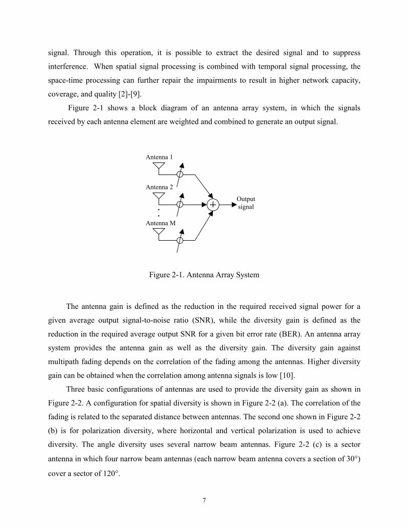
Figure 2-1 shows a block diagram of an antenna array system, in which the signals
received by each antenna element are weighted and combined to generate an output signal.
Figure 2-1. Antenna Array System
The antenna gain is defined as the reduction in the required received signal power for a
given average output signal-to-noise ratio (SNR), while the diversity gain is defined as the
reduction in the required average output SNR for a given bit error rate (BER). An antenna array
system provides the antenna gain as well as the diversity gain. The diversity gain against
multipath fading depends on the correlation of the fading among the antennas. Higher diversity
gain can be obtained when the correlation among antenna signals is low [10].
Three basic configurations of antennas are used to provide the diversity gain as shown in
Figure 2-2. A configuration for spatial diversity is shown in Figure 2-2 (a). The correlation of the
fading is related to the separated distance between antennas. The second one shown in Figure 2-2
(b) is for polarization diversity, where horizontal and vertical polarization is used to achieve
diversity. The angle diversity uses several narrow beam antennas. Figure 2-2 (c) is a sector
antenna in which four narrow beam antennas (each narrow beam antenna covers a section of 30°)
cover a sector of 120°.
Output signal
Antenna 1
Antenna 2
Antenna M
.
.

8
(a) Spatial diversity (b) Polarization diversity (c) Angle diversity
Figure 2-2. Antenna Diversity
A linear antenna array is a uniformly spaced antenna array with identical antenna elements.
For the configuration of the spatial diversity antenna, the linear antenna array can provide the
diversity gain with the low correlation if the antennas are separated far enough (the separation is
a few or tens of carrier wavelengths). When antennas are placed in proximity, the correlation
between the antenna signals is high. In this case, the adaptive filter theory can be applied to
extract the desired signal while suppressing the interference signal [55]. To extract the desired
signal and to suppress the interference signal, complex antenna weights are used to change the
phase and the magnitude of the received signal. Consider the case where two antennas are
separated by λ/2, where λ is a carrier wavelength, and a desired signal is incident on the antenna
array with the angle of arrival θ1 and an interference signal with the angle of arrival θ2, as shown
in Figure 2-3 (a). The only difference between the desired signal (S1) received at antenna 1 and
the desired signal (S2) received at antenna 2 is the phase difference, which is πsinθ1 in this
configuration. Similarly, the phase difference between the interference signals received at each
antenna is πsinθ2. To extract the desired signal and to suppress the interference signal, the
antenna weights should satisfy the following equations.
W1* + e-jπsinθ1W2
* = 1, (2-1a)
W1* + e-jπsinθ2W2
* = 0. (2-1b)
The above two equations are derived from the following two conditions (the unity gain to the
desired signal and the zero gain to the interference signal);

9
|S1W1* + S2W2
*| = |S1W1* + S1e-jπsinθ1W2
*| = |S1||W1* + e-jπsinθ1W2
*| = |S1|, (2-2a)
|I1W1* + I2W2
*| = |I1W1* + I1e-jπsinθ1W2
*| = |I1||W1* + e-jπsinθ1W2
*| = |I1|*0 = 0. (2-2b)
The antenna weights, W1 = ½ and W2 = -½j, are found if the angles of arrival are θ1 = π/6 and θ2
= -π/6, respectively. The antenna beam pattern for this case is shown in Figure 2-3 (b), in which
the antenna beam pattern provides the gain toward the direction (θ1 = π/6) of the desired signal
and suppresses the gain towards the direction (θ2 = -π/6) of the interference signal.
(a) Antenna array with signals
(b) Antenna beam pattern
Figure 2-3. Antenna Array and Beam Pattern
antenna 2
S1S2I1I2
W1*W2
*
antenna 1
θ1θ1 θ2θ2
10
2.1.2 Smart Antenna Algorithms
There are two kinds of smart antenna schemes to compute the antenna weights and to
combine the antenna signals. The first scheme is the diversity combining, in which the antenna
signals are combined to maximize the output SNR. The second one is the adaptive combining
(in a wide sense) or the beamforming, in which the antenna weights are dynamically adjusted to
enhance the desired signal while suppressing interference signals to maximize signal to
interference plus noise ratio (SINR). The performance of the adaptive combining is sometimes
limited under certain circumstances, such as when the angular separation between desired signal
and interference is small or the noise level is high [9].
There are four basic schemes in the diversity combining technique: selection diversity,
switched diversity, equal gain combining, and maximal ratio combining. Selection diversity (SD)
is the simplest method of all, in which a diversity branch having the highest SNR is selected and
directed to the output. It is also called selection combining (SC). The switched diversity does not
switch the branch until the SNR or the signal strength of the currently selected branch becomes
lower than a given threshold. The maximal ratio combing (MRC) scheme weights each antenna
signal by its SNR before combining. The MRC provides the maximal output SNR and is hence
called MRC. The MRC achieves high performance, but it is difficult to accurately compute the
SNR of each antenna signal. The equal gain combining (EGC) scheme simply adds each antenna
signal with an equal weight. For example, each antenna signal is weighted by 1/M for an M-
element antenna array.
The mean SNRs of three diversity combining schemes are presented in Table 2-1, where a
diversity combiner with M diversity branches (antennas) is employed, in which each diversity
branch has a mean SNR ΓΓΓΓ [10]. For reference, the mean SNRs with two diversity branches
(antennas) are also provided in the table.

11
Table 2-1. Mean SNR with a Diversity Combining [10]
Diversity Scheme M Branches Two Branches (M = 2)
MRC MΓΓΓΓ 2ΓΓΓΓ (3 dB)
EGC ])([
411
π−+ M ΓΓΓΓ
1.785ΓΓΓΓ (2.52 dB)
SD ∑
=
M
k k1
1 ΓΓΓΓ 1.5ΓΓΓΓ (1.76 dB)
An adaptive antenna array continuously adjusts its antenna weights by means of a feedback
control. Sometimes, it is called a smart antenna in a narrow sense. Several criteria can be used to
compute antenna weights for the adaptive combining. The criteria include maximum SINR,
minimum mean square error (MMSE), minimum variance, and least square (LS) [56]. All criteria
intend to maximize the output SINR under various assumptions. When only noise is considered,
the adaptive antenna performs the same task as the diversity antenna with the MRC. In the
presence of strong interference, the adaptive antenna shows a better performance compared with
the diversity antenna with the MRC even if the number of interferences is greater than the
number of antennas [57]. There are two kinds of beamforming systems: multibeam antenna and
adaptive combining (in a narrow sense). The multibeam antenna system selects one fixed beam
among the multiple pre-defined beams, which offers the maximum output SINR. Even though
multibeam antenna system adaptively selects the beam pattern, it provides non-uniform gain and
limited interference suppression [4] since the beam pattern is pre-defined and the number of
beam patterns is limited. Meanwhile, the adaptive combining system adaptively and freely
changes its antenna beam pattern by tracking the antenna weights. The adaptive combining
system with M antennas can form up to M-1 nulls to cancel up to M-1 interference signals [58].
The antenna weights must adapt fast enough to track the fading of the desired and interfering
signals. However, the antenna weights must also change much more slowly than the data rate.
Two approaches are used to compute the antenna weights that maximize the output SINR
for the adaptive combining (in a narrow sense). The first approach is to obtain the antenna
weights by computing the direct matrix inversion. Wiener filter belongs to this approach [55].
The second one is to obtain the antenna weights by computing the weights recursively or

12
adaptively. The steepest-descent method and the least-mean-square algorithm belong to the
second approach [55].
According to Wiener filter theory, the optimum antenna weights, wo, are obtained by
wo = R-1p, (2-3)
where R is the correlation matrix of the input vector of antenna signals and p is the cross-
correlation vector between the input vector and the desired response. This algorithm requires
computation of the matrix inversion, which results in high system complexity. The steepest-
descent method is a gradient-based adaptation algorithm [55], in which the antenna weights are
recursively obtained as following:
w(n+1) = w(n) + µ[p – Rw(n)], (2-4)
where w(n) is the antenna weight vector, µ is the step size, and R and p are the same as the
above ones.
The most widely used adaptive algorithm is based on the least-mean-square (LMS)
algorithm, in which antenna weights are recursively obtained to minimize the mean square error
using the following equations:
w(n+1) = w(n) + µu(n)e*(n), (2-5a)
e(n) = d(n) - y(n), and (2-5b)
y(n) = wH(n)u(n), (2-5c)
where u(n) is the input vector of the antenna signals and e(n) is the error signal between the
desired response d(n) and the weighted antenna output y(n) (* represents a complex conjugation
and H represents a Hermitian operation–transposition and complex conjugation). If the step size µ
is chosen such that 0 < µ < 2/P (where P is the sum of powers of each antenna input signal), the
algorithm guarantees the convergence of the antenna weights. The most benefit of the LMS
algorithm is its simplicity compared to other adaptive algorithms.
The LMS algorithm, however, suffers from a gradient noise amplification problem if the
input signal u(n) is large, i.e., the correction term µu(n)e*(n) is large. To circumvent the problem,
the following normalized LMS (N-LMS) algorithm is usually used:
w(n+1) = w(n) + 2(n)µ
uu(n)e*(n), (2-6)
13
where µ is a step size in the range of 0 < µ < 2. The N-LMS algorithm exhibits a faster rate of
convergence and better stability than the ordinary LMS algorithm for both uncorrelated and
correlated input data [55].
When the adaptive algorithm is applied to a wireless communication system, the circuit
complexity of the adaptive algorithm is an important factor to select the algorithm. It is a
particularly important factor for mobile handsets, since low complexity is highly desirable for
handsets. Due to the simplicity of the algorithm, the LMS algorithm and the N-LMS algorithm
are widely used for the adaptive antenna array systems [59],[60].
2.1.3 Smart Antennas at Handsets
Because of concerns with high system complexity and high power consumption, smart
antenna techniques have been considered primarily for base stations so far [11]-[18]. A common
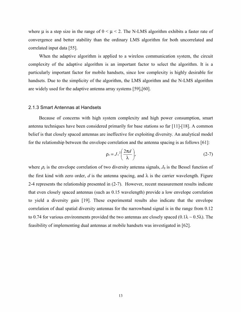
belief is that closely spaced antennas are ineffective for exploiting diversity. An analytical model
for the relationship between the envelope correlation and the antenna spacing is as follows [61]:
λπ=ρ dJe
220 , (2-7)
where ρe is the envelope correlation of two diversity antenna signals, J0 is the Bessel function of
the first kind with zero order, d is the antenna spacing, and λ is the carrier wavelength. Figure
2-4 represents the relationship presented in (2-7). However, recent measurement results indicate
that even closely spaced antennas (such as 0.15 wavelength) provide a low envelope correlation
to yield a diversity gain [19]. These experimental results also indicate that the envelope
correlation of dual spatial diversity antennas for the narrowband signal is in the range from 0.12
to 0.74 for various environments provided the two antennas are closely spaced (0.1λ ~ 0.5λ). The
feasibility of implementing dual antennas at mobile handsets was investigated in [62].

14
0 0.1 0.2 0.3 0.4 0.5 0.6 0.7 0.8 0.9 10
0.1
0.2
0.3
0.4
0.5
0.6
0.7
0.8
0.9
1
Antenna spacing (d/λ)
Env
elop
e co
rrela
tion
( ρe)
Figure 2-4. Envelope Correlation versus Antenna Spacing
The 3GPP [24] requires antenna diversity at base stations and optionally at mobile stations
[25]. Antenna diversity is also applied to the IEEE 802.11 wireless local area network (WLAN)
system [27]. Recently, the smart antenna technique has been applied to mobile terminals [20]-
[23].
The high data rate (HDR) system (adopted as IS-856 and also known as 1xEV DO)
developed by Qualcomm employs dual antennas at a mobile station [20]. Each antenna signal
was applied to its own rake receiver that combines signals from different multipaths as shown in
Figure 2-5. Then, maximal ratio diversity combining was used to combine the two rake receiver
signals. The increase of the throughput was reported in [20]. The average throughput for outdoor
stationary users was around 750 kbps with a single antenna and 1.05 Mbps with dual antennas.
The average throughput for mobile users was around 500 kbps with a single antenna and 900
kbps with dual antennas [20].

15
Figure 2-5. Dual Antenna System for the HDR
A dual antenna system for handsets was also applied to the digital European cordless
telephone (DECT) system for the indoor radio channel [21]. Figure 2-6 shows the block diagram
of the system. The dual antenna handset receiver selects one of the two signals of the receivers
based on the SINR. Each receiver processes a signal that is an equal combination of the signal
from one antenna and the phase-shifted signal from the other antenna. It was reported that
transmit power for the dual antenna system was reduced by 9 dB at the coverage of 99% for
normal walking speed (around 5 km/h) compared with the single antenna system [21].
Figure 2-6. Smart Antenna Handsets for the DECT System
Variable phase shifter
EGC
Receiver
Micro-
controller
Variable phase shifter
EGC
Receiver
Data
switch Output
Rake receiver
Rake receiver
MRC
Rake finger
Output
16
Wong and Cox proposed a dual antenna system which could be applied to handheld
devices as well as base stations [22],[23]. Summing the signals from two antennas with proper
weights in complex number cancels the dominant interference and hence increases the signal-to-
interference ratio (SIR). To compute the antenna weights, a technique to optimize the SIR was
proposed. Unlike the above two methods, the signal weighting and summing was implemented at
the radio frequency (RF) level instead of at the baseband signal level. Thus, it reduces the
complexity of the diversity combiner since it requires only one baseband processor. Computer
simulation results show that the improvement of their method in the SIR was more than 3.8 dB
compared with the conventional two-antenna selection diversity system [22],[23].
One of key features in a 3G cellular system is a high data rate. For a high data rate, a lower
BER and a smaller spreading factor are required. Thus, higher transmitting power at a base
station is necessary, which results in increased interferences to the cell. By applying smart
antenna techniques to handsets, the received SINR at handsets can be improved. Thus, the base
station transmits less power to a smart antenna handset than a conventional single antenna
handset.
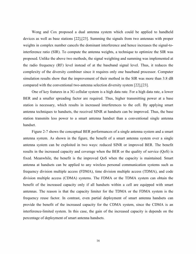
Figure 2-7 shows the conceptual BER performances of a single antenna system and a smart
antenna system. As shown in the figure, the benefit of a smart antenna system over a single
antenna system can be exploited in two ways: reduced SINR or improved BER. The benefit
results in the increased capacity and coverage when the BER or the quality of service (QoS) is
fixed. Meanwhile, the benefit is the improved QoS when the capacity is maintained. Smart
antenna at handsets can be applied to any wireless personal communication systems such as
frequency division multiple access (FDMA), time division multiple access (TDMA), and code
division multiple access (CDMA) systems. The FDMA or the TDMA system can obtain the
benefit of the increased capacity only if all handsets within a cell are equipped with smart
antennas. The reason is that the capacity limiter for the TDMA or the FDMA system is the
frequency reuse factor. In contrast, even partial deployment of smart antenna handsets can
provide the benefit of the increased capacity for the CDMA system, since the CDMA is an
interference-limited system. In this case, the gain of the increased capacity is depends on the
percentage of deployment of smart antenna handsets.

17
Figure 2-7. Smart Antenna System versus Single Antenna System
2.2 Third Generation Wireless Personal Communication Systems
The CDMA technology will proliferate as the next generation wireless personal
communication systems [63],[64]. There are two proposed wideband CDMA systems as the third
generation (3G) standards, which meet the International Telecommunication Union (ITU)
International Mobile Telecommunications (IMT)-2000 requirements. The first standard is the
Wideband CDMA (WCDMA) system, often called Third Generation Partnership Project
(3GPP)[24], that was proposed by Europe and Japan. The 3GPP system was designed to be
backward compatible with the Global System for Mobile communication (GSM) system, which
is a second generation TDMA standard deployed in Europe. The second standard is the
cdma2000 system [65] proposed by Telecommunications Industry Association (TIA). The
cdma2000 system is evolved from IS-95, which is a second generation CDMA standard
deployed in the North America and Korea. For the 3GPP system, there are two modes for the
radio access technologies: a time division duplex (TDD) mode and a frequency division duplex
(FDD) mode. The 3GPP system with the FDD mode is a CDMA system, but the 3GPP system
Received SINR
BER
Single antenna system
Smart antenna system
Reduced SINR
Improved QoS

18
with the TDD mode is a combined system of CDMA and TDMA. We consider the 3GPP system
with the FDD mode in this dissertation. Hereafter, we will refer to the 3GPP system with the
FDD mode as the 3GPP system.
Both the 3GPP system and the cdma2000 system are based on CDMA. However, they are
different in chipping rate, spreading code, forward error correction, and others. The most
prominent difference between the 3GPP system and the cdma2000 system lies in the
synchronization. For the cdma2000 system, all base stations are synchronized, i.e., the system
clock of each base station is synchronized to the global positioning system (GPS) clock. So the
cdma2000 system is called a synchronous system. Meanwhile, the system clocks used in the
3GPP base stations do not need to be synchronized. Thus, it is called an asynchronous system.
Both the 3GPP system and the cdma2000 system continuously provide a common pilot signal in
the forward link from the base station to a mobile station. The pilot signal is used to estimate the
channel condition, including the signal strength and the phase. This information is used to
coherently combine multipath signals.
2.2.1 The 3GPP System
A simple block diagram of a downlink transmitter for the 3GPP system is shown in Figure
2-8. Each bit of physical channels (PCH) is quadrature phase shift keying (QPSK) modulated.
The modulated I (in-phase) and Q (quadrature) bits are channelized by multiplying orthogonal
variable spreading factor (OVSF) codes at the chipping rate of 3.84 Mcps. All channelized
signals are combined first and then scrambled by a complex long code, which is generated from
the Gold code set. The scrambled signal and the unscrambled signal of the synchronization
channel (SCH) are combined together. The combined signal is pulse-shaped by a root-raised
cosine FIR filter with a roll-off factor of α = 0.22. The shaped signal is transmitted through the
wireless channel. A detailed description of the 3GPP WCDMA system is available in [24] and
[25].

19
Figure 2-8. Block Diagram of a Downlink Transmitter for the 3GPP System
The transmitted signal s(t) with K users can be represented in the complex form as
s(t) = [α0d0(t)Cch,0(t) + α1d1(t)Cch,1(t) + … + αKdK(t)Cch,K(t)] Sdl(t), (2-8)
where αk, dk(t), and Cch,k(t) are parameters that represent signal strength, user data, and an OVSF
code for each user k (k = 1, 2, …, K). Sdl(t) is a scramble code for the signal s(t). Note that the
first term in (2-8) is for the common pilot channel (CPICH), where d0(t) represents the fixed pilot
symbol (1+i) in QPSK format (i denotes the imaginary unit).
The received signal r(t) at the mobile station receiver is represented as
r(t) = ∑=
M
mmS
12 ξm(t)s(t-τm) + I(t) + n(t), (2-9)
where M is the number of multipaths, Sm is the average received signal power associated with the
mth path, ξm(t) is the complex channel gain for the mth multipath component with time delay τm,
I(t) is interferences from adjacent cells, and n(t) is a background noise [57]. A rake receiver
despreads received multipath signals and coherently combines them. The coherent combining of
multipath signals necessitates each multipath signal to be multiplied by the channel coefficient
estimated from the despread CPICH signal.
The pilot signal (k = 0) for the mth multipath is despread as shown below:
y0,m(n) = ∫τ++
τ+
m
m
p
pp
T1nnTT
)(1 r(t)[Sdl(t-τm)Cch,0(t-τm)]*dt, (2-10)
Σ FIR filter
PCH1
PCHk
. . .
SCH S/P
S/P
OVSF1
OVSFk
Scramble code
real or scalar complex or vector

20
where Tp is the pilot symbol period, n is the symbol index, and the symbol * represents the
complex conjugation. The kth user signal (k = 1, 2, …, K) for the mth multipath is despread in the
same manner as shown in (2-10) and is given in (2-11).
yk,m(n) = ∫τ++
τ+
m
m
k
kk
T1nnTT
)(1 r(t)[Sdl(t-τm)Cch,k(t-τm)]*dt, (2-11)
where Tk is the data symbol period of the kth user.
Then, the user signal from each multipath yk,m(n) is coherently combined to produce an
output signal as shown below:
zk(n) = ∑=
L
m 1
yk,m(n) y0,m*(n), (2-12)
where L is the number of rake fingers (which is equal to or smaller than the number of multipaths
M). It should be noted that if the spreading factor of the kth user signal SFk is smaller than that of
the pilot signal SFp, then the same pilot signal y0,m(n) is applied to obtain the
=
k
p
k
p
TT
SFSF
successive user signal outputs.
2.2.2 The cdma2000 System
Figure 2-9 shows a block diagram of a typical forward link of the cdma2000 system. One
frame of user data bits is randomly generated with a variable traffic data rate of 9600 bps, 4800
bps, 2700 bps, or 1500 bps. The generated data bits are appended with cyclic redundancy check
(CRC) and tail bits. The data bits are convolutional coded with the rate of ¼ and the constraint
length of 9 and block interleaved. Then, data bits are parallelized for QPSK data modulation, and
each parallel data bit is spread by Walsh code with the spreading factor of 64 and the chipping
rate of 1.2288 Mcps. The resultant data signal is added with the pilot signal, the paging signal,
the sync signal, and all the other users’ signals. The added signal is quadrature modulated by two
short-PN sequences and up-sampled by 8, and then is applied to shaping filters. The shaped
signal is transmitted through the channel.
The received signal is shaped back and down-sampled by 8. A four-finger rake receiver
despreads each multipath signal and combines the despread multipath signals. The despread and
combined signal is applied to the channel decoder consisting of a block deinterleaver, a Viterbi
decoder, and a CRC decoder. A detailed description of the cdma2000 system is available in [65].

21
Figure 2-9. Forward Link of the cdma2000 System
2.3 Channel Model
Because the channel model influences the design of receivers and their performance,
channel modeling is important for evaluation of a smart antenna system. In the uplink of the 3G
systems, each user signal is transmitted asynchronously and traverses different paths from the
mobile station to the base station. Thus, the main source of interference is coming from other
users’ signals within the same cell (intra-cell interference). However, in the downlink of the 3G
systems, the signal transmitted from the base station is the superposition of all active users’
signals and common control signals. The desired user signal and multiple access interference
signals traverse the same paths, but they are inherently orthogonal with each other. So it does not
pose a serious problem at handsets.
A multipath signal is effectively an interference signal to another multipath signal.
However, a rake receiver can manage multipath signals to its advantage to improve the quality of
received signal. Another source of interference in the downlink is coming from adjacent cells
(inter-cell interference), which can have a substantial impact on the performance. Note that the
Rake receiver
Channel decoding
Decoded data Demod.
- Carrier freq.: 2.0 GHz- Six multipaths
- Shaping filter - 8x down sampling
- Four rake fingers - Maximal ratio combining
- Deinterleaving - Viterbi decoding - CRC and tail bits
Channel
Data generation
Channel coding Spreading
Pilot, paging, sync, other traffic signals
Modulation
- Frame basis data generation
- CRC and tail bits - Conv. coding (R=1/4, K=9) - Block interleaving
- QPSK data mod. - Walsh code - Spread factor: 64 - Chip rate: 1.2288 Mcps
- Quad. spreading mod. - Two short-PN codes - 8x up sampling - Shaping filter

22
latter case becomes manifest when the soft handover occurs. Since the number of adjacent base
stations and hence the number of interference signals from these base stations is small, a dual
antenna system is a good candidate to combat such interference. It should be noted that a
receiver with M antennas can suppress M-1 interfering signals [58].
For a wireless channel model, three components are considered for a typical variation in the
received signal level [66]. The three components are mean path loss, lognormal fading (or slow
fading), and Rayleigh fading (or fast fading), as shown in Figure 2-10. Both theoretical and
measurement based models indicate that an average received signal level decreases
logarithmically with distance (which is the mean path loss). The difference in path loss at
different locations at the same transmitter-receiver distance is modeled as a lognormal random
variable (which is the lognormal fading). Reflections due to many scatters in the vicinity of the
receiver cause the received signal to be time varying, in which the envelope of a multipath signal
follows a Rayleigh distribution (which is the Rayleigh fading). A channel model also needs to
consider these spreads: i) delay spread due to multipath propagation, ii) Doppler spread due to
mobile motion, and iii) angle spread due to scatter distribution.
Figure 2-10. Variation of Received Signal Level
Based on the narrowband model for the signal received by an antenna array, a small time
delay between two antennas can be modeled as a simple phase shift. Consider a case where a
Distance (log)
Signal
level
(dB)
Mean path loss
Lognormal fading
Rayleigh fading

23
signal r(t) arrives at the linear antenna array as shown in Figure 2-11. Then, the received signals,
x1(t) and x2(t), at two adjacent antennas, have a phase difference. If the signal is incident on the
antenna array with the angle of arrival (θ), then the phase difference between the two received
signals is 2πdsinθ/λ, where d is the antenna spacing, λ is the wavelength of the carrier, and θ is
the angle of arrival.
Figure 2-11. Phase Difference in the Linear Antenna Array
To obtain the channel profile (such as delay, average power, and angle of arrival of each
multipath signal), not only a channel model based on statistical properties of the channel, but
also a channel model based on measurement data should be considered. For a statistical channel
model, the geometrically based single bounce (GBSB) circular and elliptical models [34],[36] are
applied. Meanwhile, the ITU channel profiles [37] are applied for the measurement based
channel model. A statistical channel model is useful in simulating a different channel
environment, in which multipath parameters are changed depending on the position of the
scatters. Even though multipath parameters are fixed in a measurement based channel model, it
is useful to reflect the real operating channel conditions.
2.3.1 GBSB Model
There are two types of the GBSB models, circular and elliptical. The GBSB circular model
is applicable for macrocell environments found in rural or suburban areas. Meanwhile, the GBSB
d
θ dsinθ
incident planewave signal,
r(t)
x1(t)x2(t)
24
elliptical model is applicable for microcell environments found in urban areas. The GBSB
models assume that multipath signals are created by single reflections of scatters, which are
uniformly distributed in a predefined elliptical and circular geometry. Delays, average power
levels, and angles of arrival (AOAs) of each multipath signal are determined from the locations
of scatters.
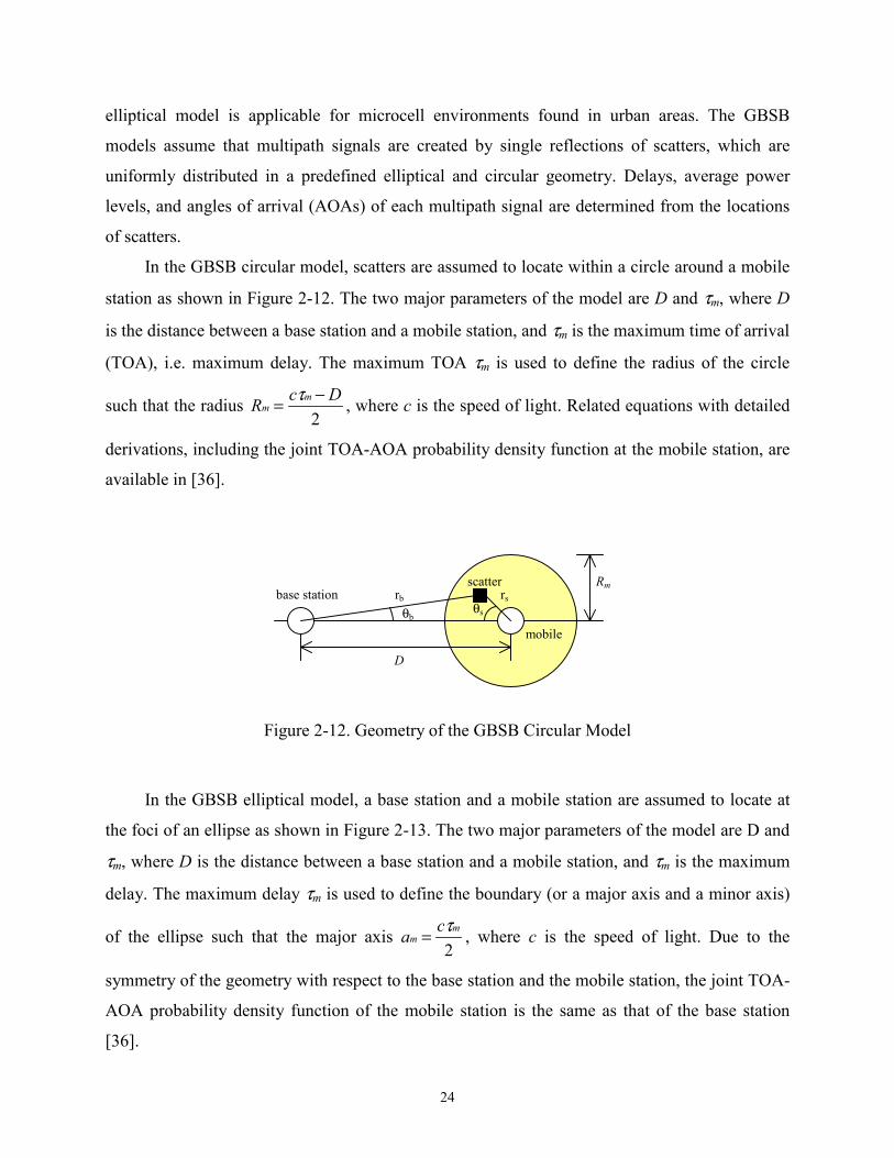
In the GBSB circular model, scatters are assumed to locate within a circle around a mobile
station as shown in Figure 2-12. The two major parameters of the model are D and τm, where D
is the distance between a base station and a mobile station, and τm is the maximum time of arrival
(TOA), i.e. maximum delay. The maximum TOA τm is used to define the radius of the circle
such that the radius 2
DcR mm
−= τ , where c is the speed of light. Related equations with detailed
derivations, including the joint TOA-AOA probability density function at the mobile station, are
available in [36].
Figure 2-12. Geometry of the GBSB Circular Model
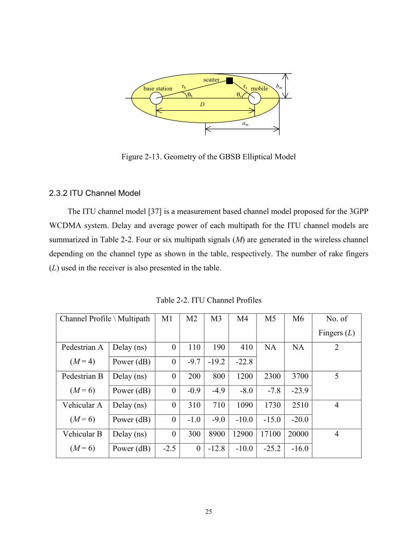
In the GBSB elliptical model, a base station and a mobile station are assumed to locate at
the foci of an ellipse as shown in Figure 2-13. The two major parameters of the model are D and
τm, where D is the distance between a base station and a mobile station, and τm is the maximum
delay. The maximum delay τm is used to define the boundary (or a major axis and a minor axis)
of the ellipse such that the major axis 2
mm
ca τ= , where c is the speed of light. Due to the
symmetry of the geometry with respect to the base station and the mobile station, the joint TOA-
AOA probability density function of the mobile station is the same as that of the base station
[36].
rb rs
θbθs
D
base station
mobile
Rm scatter
25
Figure 2-13. Geometry of the GBSB Elliptical Model
2.3.2 ITU Channel Model
The ITU channel model [37] is a measurement based channel model proposed for the 3GPP
WCDMA system. Delay and average power of each multipath for the ITU channel models are
summarized in Table 2-2. Four or six multipath signals (M) are generated in the wireless channel
depending on the channel type as shown in the table, respectively. The number of rake fingers
(L) used in the receiver is also presented in the table.
Table 2-2. ITU Channel Profiles
Channel Profile \ Multipath M1 M2 M3 M4 M5 M6 No. of
Fingers (L)
Delay (ns) 0 110 190 410Pedestrian A
(M = 4) Power (dB) 0 -9.7 -19.2 -22.8
NA NA 2
Delay (ns) 0 200 800 1200 2300 3700 Pedestrian B
(M = 6) Power (dB) 0 -0.9 -4.9 -8.0 -7.8 -23.9
5
Delay (ns) 0 310 710 1090 1730 2510 Vehicular A
(M = 6) Power (dB) 0 -1.0 -9.0 -10.0 -15.0 -20.0
4
Delay (ns) 0 300 8900 12900 17100 20000 Vehicular B
(M = 6) Power (dB) -2.5 0 -12.8 -10.0 -25.2 -16.0
4
rb rs
θb θs
D
base station mobile bm
am
scatter

26
2.4 Low-Power VLSI Design
There have been two main drives for low-power VLSI design. One drive is the increased
market demand for portable electronics powered by batteries, and the other is the advanced
processing technology [68]. For portable electronics such as cellular handsets, longer operation
time without replacing/recharging batteries is highly desirable. Low-power design is a key issue
for such applications. As the processing technology advances, the device density increases and
the feature size decreases, which in turn causes high power dissipation. High power dissipation
causes a problem for the packaging and for the reliable operation. It is especially true for high
performance microprocessor design.
The power dissipation of static CMOS circuits is composed of static power dissipation and
dynamic power dissipation [69]. Reverse biased PN junction current and subthreshold channel
are main sources of the static power dissipation. Meanwhile, capacitive current and short circuit
current are main sources of the dynamic power dissipation. The dominant factor for the power
dissipation in CMOS circuits is the charging/discharging of switching capacitances. Therefore,
most low-power design techniques are focused to reduce power dissipation due to capacitor
charging/discharging.
The capacitive power dissipation is given by the following well-known golden equation,
Pcap = αCLV2f (2-13)
where α is the switching activity, CL is the switching capacitance, V is the supply voltage, and f
is the operating frequency. Thus, the low-power VLSI design is to reduce one or several of the
four factors. Since the dependency of power dissipation on the supply voltage is quadratic,
reduction of the supply voltage is the most dramatic for the low-power design. However, the
supply voltage is often not under the designer’s control. Low-power design usually requires
tradeoffs between the circuit area, increased latency, and speed.
Low-power design techniques can be applied at different design abstract levels: system
level, algorithm level, architecture level, circuit/logic level, and technology level. Generally,
low-power design techniques applied at the higher design abstract level have more impact on
reducing the total power dissipation. Although many low-power design techniques have been
proposed [68],[70]-[72], some of them are specific to certain applications or systems. Thus one
should consider carefully when applying a low-power design technique to his/her own system.

27
Figure 2-14 shows the block diagram of a generic direct sequence (DS)-CDMA receiver
with L rake fingers [73]. In general, the signal processing requirements of DS-CDMA based
systems can be broken down into two broad categories, namely, chip rate processing and
symbol rate processing. All the blocks to the left of the dashed line in Figure 2-14 typically
operate at the chip rate (which is 1.2288 MHz or 3.84 MHz for the cdma2000 system or the
3GPP WCDMA system, respectively) or a small multiple thereof, whereas all the blocks to the
right of the dashed line operate at the symbol rate which is typically much lower. As noted in (2-
13), the capacitive power dissipation is proportional to the operating frequency. Hence, blocks
operating at a higher frequency dissipate more power, and hence low-power design of these
blocks has bigger impact on the overall power dissipation. This is illustrated below. Thus, the
low-power design on the blocks operated at the chip rate is a more efficient way to reduce the
power dissipated by a CDMA receiver.
Figure 2-14. Block Diagram of a DS-CDMA Receiver
Chip Rate Processing
ADC Shaping filter Rake Finger 2
Rake Finger 1
Rake Finger L
Cell Searcher
Deinterleaver
Channel decoder
CRC
AFC/Carrier Recovery
AGC & Power Control
. . .
Symbol Rate Processing
Rake Receiver

28
2.5 Generalized Selection Combining
In addition to classical diversity combining techniques, a generalized selection combining
has been proposed, investigated, and analyzed as a new diversity combining technique [38]-[50].
Instead of selecting all the branches as for the case of MRC, the generalized selection combining
(GSC) technique chooses the best m branches out of L branches depending on the SNR or the
signal strength and coherently combines them. The GSC is also called hybrid SC/MRC. The
number of selected branches m is decided a priori for the original GSC [38]-[50], while it varies
dynamically in [51]-[53]. For the latter approach, selection of branches whose SNRs are larger
than a given threshold is proposed in [51] and [52], and it is called absolute threshold GSC
(AT-GSC). Alternatively, selection of a branch whose relative SNR over the maximum SNR
among all branches, maxSNR
SNRi , is larger than a threshold is proposed in [51] and [53]. This method
is called normalized threshold GSC (NT-GSC).
We investigate the characteristics of the three GSC methods, the original GSC, the AT-
GSC, and the NT-GSC. It is assumed that the instantaneous SNR γi of a branch i is known and γ1
≥ γ2 ≥ … ≥ γL for a rake receiver with L branches.
The original GSC denoted as GSC (m, L) selects the best m branches out of L branches
where m is fixed, and its combined SNR is obtained as ∑=
γm
ii
1
. The combined SNR of the original
GSC is upper and lower bounded by GSC (L, L) and GSC (1, L), respectively. GSC (L, L) and
GSC (1, L) are, in fact, the MRC and the SC.
The AT-GSC denoted as AT-GSC (Ta, L) selects a branch whose SNR γi is larger than a
given threshold Ta, i.e., it finds m such that γm ≥ Ta and γm+1 < Ta. The maximal SNR for the AT-
GSC is AT-GSC (0, L), which is the MRC. The NT-GSC denoted as NT-GSC (Tn, L) selects a
branch i whose normalized SNR 1γ
γi is larger than a given threshold Tn. Note that γ1 is the
maximal SNR of among all the branches and 0 ≤ Tn ≤ 1. The NT-GSC selects m branches such
that 1γ
γm ≥ Tn and 1
1
γγ +m < Tn. The upper and the lower bounds of the SNR for the NT-GSC are
NT-GSC (0, L) and NT-GSC (1, L), respectively. Note that NT-GSC (0, L) and NT-GSC (1, L)
29
are the MRC and the SC, respectively. For comparison, characteristics of each GSC technique
are summarized in Table 2-3.
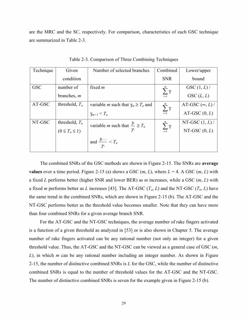
Table 2-3. Comparison of Three Combining Techniques
Technique Given
condition
Number of selected branches Combined
SNR
Lower/upper
bound
GSC number of
branches, m
fixed m ∑
=
γm
ii
1
GSC (1, L) /
GSC (L, L)
AT-GSC threshold, Ta variable m such that γm ≥ Ta and
γm+1 < Ta ∑
=
γm
ii
1
AT-GSC (∞, L) /
AT-GSC (0, L)
NT-GSC threshold, Tn
(0 ≤ Tn ≤ 1) variable m such that
1γγm ≥ Tn
and 1
1
γγ +m < Tn
∑=
γm
ii
1
NT-GSC (1, L) /
NT-GSC (0, L)
The combined SNRs of the GSC methods are shown in Figure 2-15. The SNRs are average
values over a time period. Figure 2-15 (a) shows a GSC (m, L), where L = 4. A GSC (m, L) with
a fixed L performs better (higher SNR and lower BER) as m increases, while a GSC (m, L) with
a fixed m performs better as L increases [43]. The AT-GSC (Ta, L) and the NT-GSC (Tn, L) have
the same trend in the combined SNRs, which are shown in Figure 2-15 (b). The AT-GSC and the
NT-GSC performs better as the threshold value becomes smaller. Note that they can have more
than four combined SNRs for a given average branch SNR.
For the AT-GSC and the NT-GSC techniques, the average number of rake fingers activated
is a function of a given threshold as analyzed in [53] or is also shown in Chapter 5. The average
number of rake fingers activated can be any rational number (not only an integer) for a given
threshold value. Thus, the AT-GSC and the NT-GSC can be viewed as a general case of GSC (m,
L), in which m can be any rational number including an integer number. As shown in Figure
2-15, the number of distinctive combined SNRs is L for the GSC, while the number of distinctive
combined SNRs is equal to the number of threshold values for the AT-GSC and the NT-GSC.
The number of distinctive combined SNRs is seven for the example given in Figure 2-15 (b).

30
(a) Original GSC
(b) AT-GSC or NT-GSC
Figure 2-15. Combined SNR for GSC, AT-GSC, and NT-GSC
It is possible for the AT-GSC that the maximal SNR is smaller than the threshold, so that
none of the finger is selected. Even if all the fingers are turned off momentarily, it may be able to
meet the required BER. However, such an occasion should be avoided to prevent burst errors
that are difficult to correct for a channel decoder. For practical operation, we need to modify the
selection rules for the AT-GSC as follows. A branch with maximal SNR is always selected, even
if the maximal SNR is smaller than a given threshold. In this case, the minimal SNR AT-GSC
(∞, L) becomes the SC.
Average branch SNR
GSC (1, 4)
GSC (4, 4)
GSC (3, 4)
GSC (2, 4)
Comb. SNR
Required SNR
Average branch SNR
Comb. SNR
Required SNR
T-GSC (T7, 4)
T-GSC (T1, 4)T-GSC (T2, 4)
.
.
.

31
2.6 Monte Carlo Simulation
Monte Carlo statistical method is used to determine the BER of a digital communication
system [74]. Consider we want to measure the BER of a communication system via simulation.
We should simulate the transmission of N bits and count the number of erroneous bits at the
receiver. Let )(NNe be the number of errors counted in a simulation of N bits. Then, the BER is
estimated as
N
NNNP ee
)()(ˆ = . (2-14)
According to the law of large numbers, the true BER can be obtained as )(ˆlim NPP eN
e∞→
= .
However, simulating an infinite number of bits in order to determine eP is impractical. If we
want to the estimate of the BER to be within βx100 % of the true value with the probability of 1-
α, then the number of bits necessary for simulation is obtained as follows [75].
21 21
=
−
βα )/(Q
PN
e
, (2-15)
where 1−Q is the inverse function of the Q -function. To determine the number of simulation
bits, the quantity eP should be estimated. For a large N, we can assume that ee PNP ≈)(ˆ . Then,
the number of errors is obtained using (2-14) and (2-15) and is as follows.
21 2
==
−
βα )/()]([ QNPNNE ee . (2-16)
Thus, the simulation can be stopped when the number of errors given in (2-16) is reached. For
example, 61536221
.)/( =
βα−Q when α = 0.05 and β = 0.05. This implies that if we count
about 1537 errors, then we can be assured with 95 % confidence that the estimate is within 5 %
of the true value. For reference, some representative numbers for practical simulations are
summarized in Table 2-4.

32
Table 2-4. The Number of Errors to Be Counted
α β Ne(N)
0.02 (98%) 0.02 (2%) 13530
0.02 (98%) 0.01 (1%) 54119
0.01 (99%) 0.02 (2%) 16588
0.01 (99%) 0.01 (1%) 66349
2.7 Summary
We provided preliminary studies for the proposed research in this chapter. The basic
concepts of smart antenna systems and previous works related to smart antennas at handsets were
described in Section 2.1. Two third generation wireless systems were briefly reviewed in Section
2.2. Some characteristics for a wireless channel as well as two models for a channel profile were
shortly described in Section 2.3. The fundamental concepts for low-power VLSI design were
provided in Section 2.4. A generalized selection combining method as a new diversity technique
was introduced in Section 2.5. Finally, a brief description on Monte Carlo simulation approach
was provided in Section 2.6.
These preliminary studies provided in this chapter will be a step stone of the proposed
research described in the next chapter.

33
Chapter 3 Smart Antennas at Handsets and Adaptive Rake Combining Scheme
In this chapter, we propose dual smart antennas at handsets for the 3G wireless personal
communication systems and a new combining scheme called hybrid combining. To model dual
antenna signals, several channel models are considered. We also propose a new GSC method
called minimum selection GSC and an adaptive rake combining scheme to reduce power
dissipation of a mobile rake receiver.
3.1 Smart Antennas at Handsets
We propose a dual smart antenna system incorporated into handsets for the 3G wireless
personal communication systems in which the two antennas are separated by a quarter
wavelength (3.5 cm) [28]-[32]. To investigate the performance of the proposed dual antenna
handsets, different combining schemes are exploited. To combine each multipath signal, a
diversity combining [28],[30], an adaptive combining [29],[32], and a new proposed combining
scheme called hybrid combining [31] are employed.
3.1.1 Diversity Combining
A diversity combiner combines the dual antenna signals using a diversity combining
scheme. Three diversity combining schemes—selection diversity (SD), equal gain combining
(EGC), and maximal ratio combining (MRC)—are considered. The SD scheme selects the signal
with higher power. The EGC scheme simply adds two signals with an equal weight of 0.5. The

34
MRC scheme weights each signal by its signal level and adds them according to the formula,
|||| bbaa + , where a and b are the two rake receiver outputs or the two rake finger outputs.
To process the dual antenna signals, two levels of diversity combining schemes are
considered. The first scheme is the rake level diversity combining in which a diversity combiner
combines rake receiver outputs. The second one is the finger level diversity combining in which
a diversity combiner combines finger outputs. The two schemes are shown in Figure 3-1. For
simplicity, only three fingers are depicted in the figure. It should be noted that all finger signals
are pre-weighted (according to the magnitude and phase information of the pilot signal) before a
diversity combiner combines finger outputs.
(a) Rake Level Diversity Combining
(b) Finger Level Diversity Combining
Figure 3-1. Diversity Combining
SD/ EGC/ MRC
Rake Rx 1
Rake Rx 2
r1(t)
r2(t)
Diversity combiner
Out
Rake Finger
SD/ EGC/ MRC
SD/ EGC/ MRC
SD/ EGC/ MRC
r1(t)
r2(t) Out
Rake Finger

35
3.1.2 Adaptive Combining
To combine each multipath signal from dual antennas, an adaptive combining scheme
based on the normalized least mean square (N-LMS) algorithm described in Chapter 2 is applied,
in which antenna weights are recursively obtained to minimize the mean square error. The
considered dual antenna system with the adaptive combiner (AC) is shown in Figure 3-2.
Figure 3-2. Adaptive Combining
The procedure to obtain the antenna weights is explained below. A new antenna weight
ω(j)m(n+1) for the mth multipath on the jth antenna is computed as follows [55].
ω(j)m(n+1) = ω(j)
m(n) + µ (y(j)0,m(n) /∑
=
2
1j| y(j)
0,m(n)|2) e*0,m(n), (3-1)
where ω(j)m(n) is the current antenna weight, y(j)
0,m(n) is the despread pilot signal for the mth
multipath on the jth antenna, µ is the step size in the range of 0 < µ < 2, and e0,m(n) is the error
signal. The error signal e0,m(n) is expressed as ž0,m(n) - z0,m(n), where ž0,m(n) is the desired
reference pilot signal for the mth multipath signal and z0,m(n) is the combined pilot signal. We
assume that the pilot signals from each antenna are ideally phase shifted and combined to obtain
the desired reference pilot signal. Hence, the desired reference pilot signal ž0,m(n) is obtained by
averaging the despread pilot signal such that
ž0,m(n) = Q
Q
llnln yy mm∑
−
=−+−
+
1
02
i)(12
01
0 |))(||)((| )(,
)(,
, (3-2)
Rake finger
AC
AC
AC
Output

36
where Q is the number of pilot symbols to be averaged and (1+i) is the known transmitted pilot
symbol. The combined pilot signal z0,m(n) for the mth multipath is obtained using the pilot signals
y(j)0,m(n) from each antenna and the current antenna weights ω(j)
m(n) such that
z0,m(n) = ∑=
2
1j y(j)
0,m(n)ω(j)m
*(n). (3-3)
After the antenna weights are obtained, the despread kth user signal for the mth multipath
from each antenna is weighted and combined as
zk,m(n) = ∑=
2
1j y(j)
k,m(n)ω(j)m
*(n), (3-4)
where y(j)k,m(n) is the despread kth user signal for the mth multipath on the jth antenna and ω(j)
m(n)
is the obtained antenna weight. Then, the combined user signal from each multipath zk,m(n) is
coherently combined to produce an output as shown below:
zk(n) = ∑=
L
m 1
zk,m(n) z0,m*(n), (3-5)
where L is the number of rake fingers. If the spreading factor of the kth user signal SFk is smaller
than that of the pilot signal SFp, then the same antenna weight ω(j)m(n) is applied to obtain the
k
p
SFSF
successive user data symbols.
Finally, the antenna weight should adapt fast enough to track the fading of the desired and
interfering signals, but it should be much slower than the data rate.
3.1.3 Hybrid Combining
Diversity combiner (DC) exploits the spatial diversity among multiple antenna signals and
achieves higher performance when multiple antenna signals are less correlated. An adaptive
combiner (AC) combines corresponding finger outputs of the two antennas with appropriate
antenna weights, which are recursively obtained based on the N-LMS algorithm. Since these two
combining schemes exhibit somewhat opposite and complementary characteristics, a new
combining scheme is proposed to exploit the advantages of the both schemes. As observed in
Chapter 4, the DC and the AC exhibit somewhat opposite trends in SINR and mobile velocity.
One may be tempted to select a better performing scheme (among DC and AC) based on current

37
operating environment. However, the approach is impractical, as we cannot accurately estimate
the performance or the BER of each scheme due to imprecise estimation of the SINR, and the
difficulty of measuring the mobile velocity. To circumvent these problems, we propose a simple,
yet effective, scheme called a hybrid combiner (HC). The proposed HC combines DC and AC
outputs using MRC. The block diagram of the proposed HC is presented in Figure 3-3. Since it is
difficult to compute the SNR, the instantaneous signal plus noise (S+N) value is used to weight
each combiner output instead of its SNR.
Figure 3-3. Hybrid Combiner for a Dual Antenna System
3.2 Channel Model
We assume that the dual antennas at a handset are identical, omnidirectional, and separated
with a quarter wavelength of the carrier. Among the three components to be considered for a
typical variation in the received signal level, the lognormal fading is not included in our channel
model for the 3GPP WCDMA system; this model is implemented with Matlab tool. Later, we
will include the lognormal fading in the channel model for the cdma2000 system, a model
implemented with the SPW tool.
AC
AC
AC
DC
MRC
Rake Finger
Output

38
3.2.1 Loosely and Spatially Correlated Fading Channel Models
First, we consider two types of the channel model specific to the dual antenna signals: i)
loosely correlated fading channel model (LCFCM) and ii) spatially correlated fading channel
model (SCFCM). Each antenna signal is assumed to have independent Rayleigh fading in the
LCFCM. In the SCFCM, each antenna signal is subject to the same Rayleigh fading, but is
different in the phase due to a non-zero angle of arrival (AOA). Each multipath signal has a
different AOA. It is assumed that a multipath signal has the same arrival time for the two
antennas in the channel model. The two types of the channel model are illustrated in Figure 3-4.
The signal s(t) represents the transmitted signal from the base station in the figure, and signals
r1(t) and r2(t) represent the two received antenna signals at the mobile station. A channel model
with less correlated dual antenna signals, which is the LCFCM in our model, is expected to yield
higher diversity gain [10]. We believe that the actual channel of dual antenna signals (for both
the diversity combining and the adaptive combining) lies in between these two channel models.

39
(a) Loosely Correlated Fading Channel Model
(b) Spatially Correlated Fading Channel Model
Figure 3-4. Two Types of the Channel Model
s(t)
r1(t)
r2(t)
Rayleigh fading
Rayleigh fading
Rayleigh fading
Rayleigh fading
Rayleigh fading
Rayleigh fading
Z-τ0
Z-τ1
Z-τ2
e-jφ0
s(t)
r1(t)
r2(t)
Rayleigh fadingZ-τ0
e-jφ1
Rayleigh fadingZ-τ1
e-jφ2
Rayleigh fadingZ-τ2

40
3.2.2 Envelope Correlated Fading Channel Model
Two channel models considered in the previous subsection, the LCFCM and the SCFCM,
are useful to evaluate the upper and the lower bounds of the system performance. To model the
actual channel of dual antenna signals lying in between these two channel models, we modify the
procedure developed by Ertel and Reed [33] and propose an envelope correlated fading channel
model (ECFCM).
Two Rayleigh fading antenna signals for each multipath in the ECFCM are assumed to
have an envelope correlation and a phase difference due to a non-zero AOA. It is assumed that a
multipath signal has a different AOA, but the same arrival time for the two antennas in the
channel model. The channel model with three multipath signals is illustrated in Figure 3-5.
λ
θ=φ ii
πdsin2
Figure 3-5. Envelope Correlated Fading Channel Model
The following procedure is used to obtain two antenna signals for each multipath. For a
given envelope correlation ρe, two envelope correlated Rayleigh fading signals x = [x1 x2]T are
obtained from two uncorrelated (independent) Rayleigh fading signals w = [w1 w2]T and a
coloring matrix L such as x = Lw [33]. The coloring matrix L is given as
κ−+κ= 211
21
01)(L j , (3-6)
s(t) y1(t)
y2(t)
e-jφ0
Two Rayleigh fading signals with ρe envelope correlation
Z-τ0
e-jφ1
Z-τ1
e-jφ2
Two Rayleigh fading signals with ρe envelope correlation
Z-τ2
Two Rayleigh fading signals with ρe envelope correlation

41
where κ is a parameter related to the envelope correlation ρe, and it is approximated by eρ . (A
more accurate method to obtain κ from a given ρe is described in [33].) As one may notice by
inspection, the phase difference between two obtained signals x1 and x2 is independent of an
AOA.
To make the phase difference a function of an AOA as a narrowband signal, new signals y
= [y1 y2]T can be obtained from x such that
λθ−=
= ])2)([()( 12
1
2
1 sinπdxanglejexpxabsx
yy
y , (3-7)
where d, θ, and λ are the antenna distance, the AOA, and the carrier wavelength, respectively.
The newly obtained signals y are the desired Rayleigh fading signals for each multipath with an
envelope correlation ρe and a phase difference.
Experimental results indicate that the envelope correlation ρe of dual spatial diversity
antennas for the narrowband signal is in the range from 0.12 to 0.74 for various environments
provided the two antennas are closely spaced (0.1λ ~ 0.5λ) [19]. Figure 3-6 shows examples of
envelopes and phases of two Rayleigh fading signals in the ECFCM, which are generated using
the above procedure for ρe = 0.5 and 120 Hz of Doppler frequency.

42
500 1000 1500 2000 2500 3000 3500 4000 4500-15
-10
-5
0
5
Samples
Fadi
ng E
nvel
opes
[dB
]
Antenna 1Antenna 2
(a) Envelope
500 1000 1500 2000 2500 3000 3500 4000 4500-4
-3
-2
-1
0
1
2
3
4
Samples
Pha
se [r
adia
n]
Antenna 1Antenna 2Phase Difference
(b) Phase
Figure 3-6. Two Rayleigh Fading Signals in the ECFCM
3.2.3 Procedure to Obtain Channel Profile using the GBSB Models
The following procedure is used to obtain a channel profile using the GBSB model. A
scatter is placed randomly within a predefined ellipse or circle. The distance rb between the base
station and the scatter and the distance rs between the scatter and the mobile station are obtained
from the location of the scatter. The propagation delay τ is calculated as (rb + rs)/c, where c is the

43
speed of light. Then a new scatter is placed randomly, and the propagation delay is calculated in
the same manner. If the difference between the new propagation delay and any existing
propagation delay is greater than one chip delay (which is about 260 ns for the 3GPP WCDMA
system), then the scatter is selected. Otherwise, the scatter is deleted, as the multipath signal
cannot be resolved by a rake finger. The process repeats until a predefined number of multipaths
(or scatters) is achieved. The unit average power P0 is assigned to the multipath signal with the
smallest propagation delay τ0. The average power of a multipath signal Pi, i ≠ 0 is calculated
using the mean path loss model [66] such that Pi = P0 * (τi/τ0)–n, where τi is the propagation delay
of the multipath and n is the path loss exponent. We set n to 3.5 in our simulation. The AOA of
each multipath signal is obtained from the location of the scatter and the mobile station.
Figure 3-7 illustrates examples of the channel profiles of four multipath signals obtained
through the procedure described above. The first channel profile in Figure 3-7 (a) is for the
GBSB circular model, where the distance D was set to 2000 m to simulate a rural or a suburban
environment and the maximum delay τm to 35 chips (equivalently 9.1 µs) in the process. The
second channel profile in Figure 3-7 (b) is for the GBSB elliptical model, where the distance D
was set to 800 m in consideration of an urban environment and the maximum delay τm to 20
chips (equivalently 5.2 µs) in the process. The maximum delays for the two GBSB models were
chosen, so that the time difference between the maximum delay τm and the delay for the line-of-
sight signal (= D/c) is roughly equal (which is about 9.5 chips for the 3GPP WCDMA system)
for the two models. As can be observed from the two figures, all the multipath signals of the two
models lie in the time window of around 10 chips due to the choice of maximum delays.

44
(a) GBSB Circular Model (b) GBSB Elliptical Model
Figure 3-7. Channel Profiles for the GBSB Circular and Elliptical Models
An important phenomenon for the GBSB models is that the relative distance of a multipath
signal to the first multipath signal is smaller for the circular model than the elliptical model.
Hence, this results in relatively smaller path loss, i.e., relatively larger signal power. The
phenomenon is manifest as shown in the two figures. The phenomenom leads to an important
fact. Since a multipath signal acts as interference to other multipath signals, strong multipath
signals of the circular model incur strong interference. If the noise level is low for the circular
model, the SINR is dominant by the interference. Therefore, the SINR of the circular model is
smaller than that of the elliptical model for a low noise level. It is opposite for strong noise. The
SINR of the circular model is larger than that of the elliptical model for a high noise level. The
phenomenon also explains the impact of the maximum delay in the GBSB models.
3.2.4 Channel Model Including the Lognormal Fading
In addition to the LCFCM and the SCFCM, an uncorrelated fading channel model
(UCFCM) is also considered for the cdma2000 system, in which the system model is
implemented with the SPW tool. Each antenna signal is assumed to have the same lognormal
fading in the LCFCM and the SCFCM. In the UCFCM, each antenna signal is assumed to have
not only independent Rayleigh fading but also independent lognormal fading. The UCFCM is
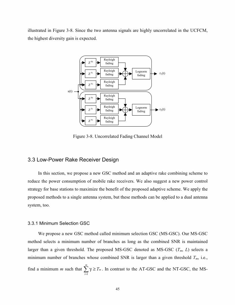
45
illustrated in Figure 3-8. Since the two antenna signals are highly uncorrelated in the UCFCM,
the highest diversity gain is expected.
Figure 3-8. Uncorrelated Fading Channel Model
3.3 Low-Power Rake Receiver Design
In this section, we propose a new GSC method and an adaptive rake combining scheme to
reduce the power consumption of mobile rake receivers. We also suggest a new power control
strategy for base stations to maximize the benefit of the proposed adaptive scheme. We apply the
proposed methods to a single antenna system, but these methods can be applied to a dual antenna
system, too.
3.3.1 Minimum Selection GSC
We propose a new GSC method called minimum selection GSC (MS-GSC). Our MS-GSC
method selects a minimum number of branches as long as the combined SNR is maintained
larger than a given threshold. The proposed MS-GSC denoted as MS-GSC (Tm, L) selects a
minimum number of branches whose combined SNR is larger than a given threshold Tm, i.e.,
find a minimum m such that m
m
iTi ≥γ∑
=1
. In contrast to the AT-GSC and the NT-GSC, the MS-
Z-τ0 Rayleigh
fading
r1(t)
r2(t)
Z-τ1
Z-τ2
Lognormfading
Rayleighfading
Rayleighfading
Z-τ0 Rayleigh
fading
Z-τ1
Z-τ2
Lognormfading
Rayleighfading
Rayleighfading
s(t)

46
GSC performs better as the threshold value becomes larger. The combined SNRs for the
proposed MS-GSC are shown in Figure 3-9 (a), and the number of distinctive combined SNRs is
equal to the number of the threshold values. The SNR of the MS-GSC for a given threshold is
ideally independent of the average branch SNRs.
For a practical implementation, the signal level or strength is used instead of a branch SNR,
which is difficult to measure. Since the received signal contains the desired signal as well as
noise, the signal strength represents signal plus noise (S+N) value. Even if the signal strength is
used for the original GSC, the AT-GSC, and the NT-GSC, the trend remains the same. However,
the trend for the MS-GSC changes as shown in Figure 3-9 (b). When the SNR of each branch is
low/high, the amount of the noise is relatively large/small. Thus, the combined (S+N) shows a
low/high SNR.

47
(a) Ideal MS-GSC
(b) Practical MS-GSC with (S+N)
Figure 3-9. Combined SNR for MS-GSC
The operation of the MS-GSC is as follows. The MS-GSC starts with a given threshold T
and an initial condition GSC (k, L). The combined signal strength is periodically measured. If the
combined signal strength is less than the threshold, then one more rake finger is activated in the
next period. Since the signal with the smaller delay is stronger in general, the finger with the
smallest delay is selected. Note that the delay information is provided by a cell searcher. If the
combined signal strength is marginally greater than the threshold, then a rake finger with the
Average branch SNR
Comb. SNR
MS-GSC with SNR
MS-GSC with (S+N)
MRC
SC
Average branch SNR
Comb. SNR
Required SNR
MS-GSC (T1, 4)
MS-GSC (T2, 4)
MS-GSC (T5, 4) ...

48
lowest signal strength is turned off in the next period. Otherwise, the current rake combining
with k fingers is maintained.
Comparing with the AT-GSC and the NT-GSC, the proposed MS-GSC has two benefits.
Since the combined signal strength in the MS-GSC is maintained constantly, the statistics of
erroneous bits have a low standard deviation, which is presented in Chapter 5. This may result in
less burst errors, which leads to a better error correction for a channel decoder. The second
benefit is that the MS-GSC enables power reduction by turning off unselected fingers. The MS-
GSC can meet the given threshold condition by turning on another finger with the smallest delay
or turning off a finger with the lowest signal strength. In contrast, the AT-GSC and the NT-GSC
necessitate activation of each finger momentarily to measure the signal strength, so that it can
determine if the signal strength is above the threshold value or not.
We also need to modify the selection rules for the MS-GSC for practical operation. The
MS-GSC selects all branches even if all combined SNR or (S+N) is smaller than a given
threshold. We apply the modified rule for our simulation in Chapter 5.
3.3.2 Adaptive Rake Combining Scheme
We determine a set of N threshold values {T(1), T(2), …, T(N)} for each GSC using a
system simulation, where each GSC performs better as the index of the threshold value increases.
This implies that T(1) > T(2) > … > T(N) for the AT-GSC and the NT-GSC and T(1) < T(2) < …
< T(N) for the MS-GSC. A larger N leads to, on average, a larger number of branches turned off,
but it results in more complex hardware and more frequent changes of threshold values.
Therefore, a larger N does not guarantee more power reduction. The SNR range of a threshold
value T(i) is the range in which the required BER is met for T(i), but not with T(i-1). The SNR
range of a threshold value T(i) is illustrated in Figure 3-10. As shown in the figure, the SNR
range for the threshold value T(i) is good enough to meet the required BER.
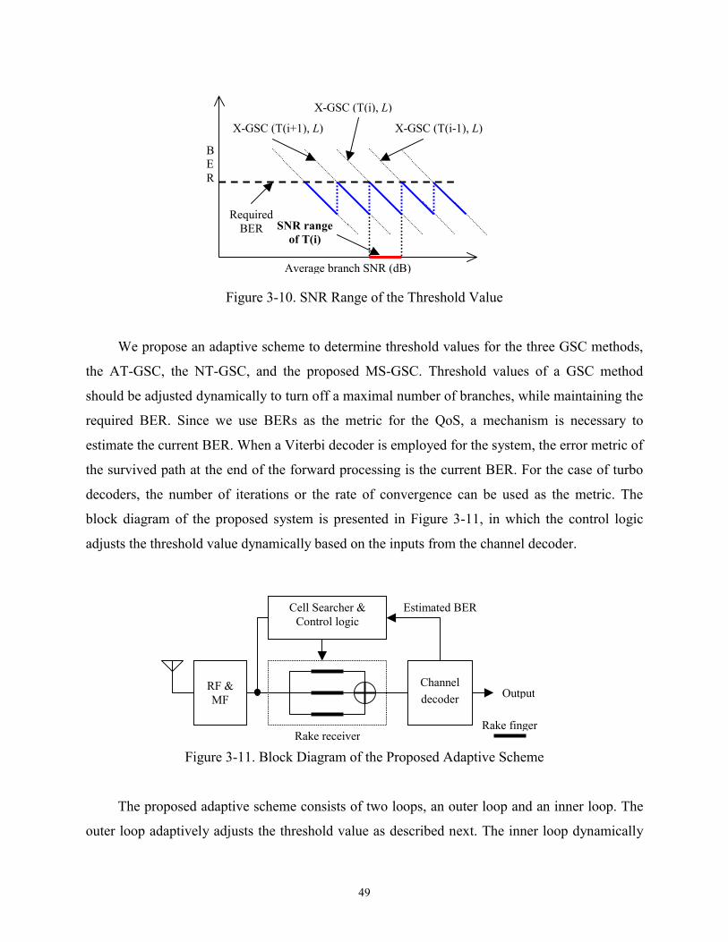
49
Figure 3-10. SNR Range of the Threshold Value
We propose an adaptive scheme to determine threshold values for the three GSC methods,
the AT-GSC, the NT-GSC, and the proposed MS-GSC. Threshold values of a GSC method
should be adjusted dynamically to turn off a maximal number of branches, while maintaining the
required BER. Since we use BERs as the metric for the QoS, a mechanism is necessary to
estimate the current BER. When a Viterbi decoder is employed for the system, the error metric of
the survived path at the end of the forward processing is the current BER. For the case of turbo
decoders, the number of iterations or the rate of convergence can be used as the metric. The
block diagram of the proposed system is presented in Figure 3-11, in which the control logic
adjusts the threshold value dynamically based on the inputs from the channel decoder.
Figure 3-11. Block Diagram of the Proposed Adaptive Scheme
The proposed adaptive scheme consists of two loops, an outer loop and an inner loop. The
outer loop adaptively adjusts the threshold value as described next. The inner loop dynamically
Average branch SNR (dB)
B E R
Required BER
X-GSC (T(i), L)
X-GSC (T(i-1), L)X-GSC (T(i+1), L)
SNR range of T(i)
Channel decoder
Rake receiver
Cell Searcher & Control logic
Estimated BER
RF & MF
Rake finger
Output

50
changes the finger selection to meet the required condition with the threshold value provided
from the outer loop.
Figure 3-12 shows the operation of the outer loop. Suppose that the current threshold of a
GSC method is T(i). Current BER is periodically estimated at the end of each frame. If the
estimated BER is higher than the required BER, then the threshold index is increased to T(i+1) in
order to lower the BER in the next frame. If the BER reaches the right end of the SNR range of
the current threshold T(i), then the threshold index is decreased to T(i-1). Otherwise, the current
threshold T(i) is maintained.
(a) Increasing a Threshold Index
(b) Decreasing a Threshold Index
Figure 3-12. Operation of GSCs
Average branch SNR (dB)
B E R
Required BER
X-GSC (T(i), L)X-GSC (T(i+1), L)
Current BER
X-GSC (T(i-1), L)
Average branch SNR (dB)
B E R
Required BER
X-GSC (T(i), L)
Current BER

51
The power saving of the proposed adaptive scheme is highly dependent on the operating
condition and the employed threshold set. The average number of rake fingers activated m is
obtained as ∑=
=N
iiiPAm
1
, where N is the number of threshold values {T(i)}, Ai is the average
number of rake fingers activated for a threshold value T(i), and Pi is the probability of the
proposed adaptive scheme operating in the SNR range of the threshold value T(i). Then, the
power saving with the proposed adaptive scheme over the MRC rake combiner is obtained as
LmL − . Thus, if we know each probability Pi, then the power saving with the proposed adaptive
scheme could be estimated. The probability Pi depends on the channel condition and the power
control strategy.
In the following, we analyze the power saving of the proposed adaptive scheme under
equal probability, i.e., Pi is equal for i = 1, 2, … N. Suppose that a threshold set is chosen such
that the difference between the average numbers of rake fingers activated for two consecutive
threshold values is δ. In other words, the average number of the rake fingers activated is 1, 1+δ,
1+2δ, …, L-δ, L for a threshold value T(1), T(2), …, T(N), respectively. Let us consider the case
of δ = 1, equivalently, N = L. Then, the probability Pi of the proposed adaptive scheme operating
in the SNR range of each threshold is L1 . Since the number of rake fingers activated for the
threshold value T(i) is i, where i = 1, 2, …, L, the average number of rake fingers activated m is
∑=
L
i Li
1
or 2
1+L . Thus, the power saving with the proposed adaptive scheme over the MRC rake
combiner is obtained as L
L2
1− .
Next, we consider the case of δ < 1 and kδ = 1 for some integer k. Each SNR range for the
case of δ = 1 is subdivided into k pieces except for the range of SNR1 in which one finger is
always turned on. Figure 3-13 shows the case of δ = 0.5 and k = 2, where the average number of
rake fingers activated with each threshold value is 1, 1.5, 2, 2.5, 3, …, L-0.5, L. Suppose that the
probability of the proposed adaptive scheme operating in each subrange with an SNRn range is
equal and is k1 . Then, the average number of rake fingers activated in each group except SNR1 is

52
obtained as 212 δ+−n , where n = 2, 3, …, L. Therefore, the overall average number of rake
fingers activated m is approximated to 2
δ+L . The derivation of the above two equations is
presented at the end this subsection. Thus, the power saving with the proposed adaptive scheme
over the MRC rake combiner is obtained as L
L2
δ− . The power saving for our scheme increases
as L increases with the maximum value of 0.5 for L = ∞. As an illustration, the power saving of
the proposed scheme is 44.5 %, 45.9 %, and 46.7 % when L is 3, 4, and 5, respectively, with δ =
0.33.
The proposed adaptive scheme can also work with the original GSC. There are only L
different SNR ranges for the original GSC. The outer loop increases or decreases the number of
rake fingers activated to maintain the required BER. Selecting additional finger or turning off
one of the currently activated fingers may follow the same operation as the MS-GSC does. The
adaptive scheme for the original GSC can be considered as a special case of other GSCs, in
which δ = 1. The power saving of the original GSC over the MRC rake combiner is L
L2
1− .
Figure 3-13. SNR Ranges with Different Threshold Sets
SNR1 SNR2SNR3SNRL
SNR1 SNR2,2SNR3,2SNRL,2 SNR2,1SNR3,1SNRL,1
Required BER
Average branch SNR (dB)
B E R
SNR ranges for δδδδ = 0.5
SNR ranges for δδδδ = 1
GSCs with δ = 1
GSCs with δ = 0.5

53
The average number of rake fingers activated in each group except the first group is
obtained as follows. The average number of rake fingers activated for each subrange of an SNRn
range is (n-1)+δ, (n-1)+2δ, …, (n-1)+kδ, where n = 2, 3, …, L. Since the probability of operating
in each subrange within an SNRn range is k1 , the average number of rake fingers activated in
each group is computed as follows.
{ })(...)()( δ+−++δ+−+δ+− knnnk
12111 (3-8a)
{ })...()( δ++δ+δ+−= knkk
211 (3-8b)
δ++−=
211 )()( kn (3-8c)
212 δ+−= n (since kδ = 1). (3-8d)
The overall average number of rake fingers activated, m , is approximated as follows. The
average number of rake fingers activated in each group is 1 (when n = 1) and 212 δ+−n (when n
= 2, 3, …, L). Since the probability of operating in each SNR range is assumed as L1 , m is
computed as follows.
δ+−++δ+−++δ++δ++= )(...)(...)()(
212
212
25
2311 Ln
Lm (3-9a)
δ+−++δ+−++δ++δ++δ+≥ )(...)(...)()()(
212
212
25
23
211 Ln
L (since 0<δ≤1) (3-9b)
δ+−+++= )()...(
2212
23
211 LL
L (3-9c)
δ+=
221 2 LLL
(3-9d)
2
δ+= L . (3-9e)
54
3.3.3 Power Control Strategy
The objective of the proposed adaptive rake combining scheme is to turn off as many
fingers as possible to reduce the power dissipation, while maintaining the required QoS. The
strategy of the conventional power control aims to maintain the received signal power level at a
mobile station, so that the signal level combined with the MRC would meet the required QoS.
Hence, the rake receiver of the mobile station dissipates the maximum power. To maximize the
benefits of the proposed rake combining method, we suggest the base station should transmit the
maximum allowable power so that the smallest number of fingers is turned on at the mobile
station. The maximum allowable power should be determined subject to the acceptable
interference to other active users in its own cell and neighboring cells.
3.4 Summary
We proposed dual smart antennas at handsets for the 3G wireless personal communication
systems in this chapter. Smart antennas at handsets with a new combining scheme called hybrid
combining were proposed in Section 3.1. To model dual antenna signals at handsets, three
channel models—LCFCM, SCFCM, and ECFCM—were considered in Section 3.2. Finally, a
new GSC method and an adaptive rake combining scheme to reduce the power consumption of
mobile rake receivers were proposed in Section 3.3. A new power control strategy for base
stations to maximize the benefit of the proposed adaptive scheme was suggested in Section 3.3,
too.
The proposed system and schemes described in this chapter will be evaluated and verified
in the following two chapters.
55
Chapter 4 Performance of Smart Antennas at Handsets
In this chapter, we present the simulation results to evaluate the performance of the
proposed dual smart antenna system at handsets for the 3G wireless personal communication
systems. Simulation results with three different combining schemes for the 3GPP WCDMA
system are presented first. Then, the simulation results of the dual smart antenna handsets for the
cdma2000 system are presented.
4.1 Performance of Diversity Combining for the 3GPP System
Simulation results to evaluate the performance of the dual smart antenna handsets with the
diversity combining scheme for the 3GPP system are presented in this section.
4.1.1 Simulation Environment
A signal from a base station propagates through the channel. The two types of the channel
model, SCFCM and LCFCM, described in Chapter 3 are employed for the simulation. The
GBSB elliptical and circular models are adopted to generate the channel profile of multipath
signals. The signals received at the dual antennas of a handset are applied to their own rake
receivers after pulse shaped by an FIR filter, as shown Figure 4-1. A diversity combiner
combines the two rake receiver outputs using a diversity combining scheme (Only the rake level
diversity combining is considered). Three diversity combining schemes, SD, EGC, and MRC,
were considered in our simulation. For the MRC, we obtain the output according to the formula,
|||| bbaa + , where a and b are the two rake receiver outputs. We call it as square law combining
(SLC).

56
Figure 4-1. Dual Smart Antenna Receiver with Diversity Combiner
In our simulation, the output of a diversity combiner is hard decided to either 1 or 0, and
compared with the original data bits to evaluate the system performance in terms of BER. For
simplicity, we modeled the interference from adjacent cells as additive white Gaussian noise
(AWGN).
The environment considered in our simulation is as follows. The following model
parameters, called baseline parameters in this section, were assumed. The distance between the
two antennas at handsets is λ/4 (3.5 cm). The distance from the desired base station to the mobile
station is 2000 m in the GBSB circular model, and the maximum multipath delay is 35 chips.
The distance from the desired base station to the mobile station is 800 m in the GBSB elliptical
model, and the maximum multipath delay is 20 chips. The mobile velocity is 60 km/hr, which
results in 119 Hz of maximum Doppler frequency for a 2.14 GHz carrier frequency. Eight users’
signals of a spreading factor 32 and the common pilot (CPICH) signal are channelized,
combined, scrambled, pulse-shaped, and transmitted through the channel. Twenty percent of the
total transmitted power is allocated to the CPICH, and the remaining 80% of the power is
divided equally and allocated to each user signal. Four multipath signals with the channel profile
obtained from the GBSB models arrive at handset antennas. A rake receiver with three rake
fingers is considered at handsets.
4.1.2 Simulation Results under the GBSB Circular Model
The GBSB circular model is employed to generate channel profiles for the simulation. The
simulation results with three diversity combining schemes and two types of the channel model
FIRfilter
FIRfilter
Rake rx
Rake rx
SD/
SLC/
EGC
Output
AWGNs
From Tx
57
are presented in Figure 4-2. Figure 4-2 (a) and (b) are the performance of the single and of the
dual antenna systems under the SCFCM and the LCFCM, respectively. The y-axis of a plot is the
BER, and the x-axis is the ratio of the symbol energy of the first multipath signal to the AWGN.
The top graph in each plot is the BER of a single antenna (SA) system. The second, the third, and
the bottom graphs are the BERs of the dual antenna system with SD, SLC, and EGC diversity
combining schemes, respectively. As can be seen from the two figures, the dual smart antenna
system always performs better than a single antenna system for both channel models. For the
dual smart antennas, the EGC performs the best among the three diversity combining schemes.
For the purpose of comparison, the performance of the dual smart antenna system with the EGC
diversity combining scheme alone under the two channel models and that of a single antenna
system is shown in Figure 4-2 (c). The performance gain of the EGC diversity combining over a
single antenna system is 3.6 dB for the SCFCM at BER = 10-1 and 4.6 dB for the LCFCM. The
performance gain increases further with a lower BER. For example, the gain is 6.4 dB for the
SCFCM at BER = 4x10⁻² and 7.5 dB for the LCFCM. As expected, the higher performance gain
is achieved under the LCFCM than the SCFCM.
It is worth noting that the BER is saturated beyond a certain level of Eb/No for both single
and dual antenna systems, i.e., the increase of the transmitter power beyond a certain level fails
to further decrease the BER. This is explained as the increased transmitter power increases the
signal level of all multipath signals, i.e., the power level of the interference signals.

58
0 5 10 15 2010-3
10-2
10-1
100
Eb/No (dB)
BE
R
SASDSLCEGC
(a) BERs under the SCFCM
0 5 10 15 2010-3
10-2
10-1
100
Eb/No (dB)
BE
R
SASDSLCEGC
(b) BERs under the LCFCM

59
0 5 10 15 2010-3
10-2
10-1
100
Eb/No (dB)
BE
R
SASCFCMLCFCM
(c) BER Bound with the EGC
Figure 4-2. BERs with Three Diversity Combining Schemes and Two Channel Models
To investigate the impact of individual parameters, we also simulated variations of several
individual parameters and present the results below. Hereafter, we consider only the EGC
diversity combining scheme for the dual smart antenna system. Firstly, we investigated the
impact of the distance of two antennas at handsets under the SCFCM. The simulation results
with the antenna distances of λ/8, λ/4, and λ/2 under the SCFCM are presented in Figure 4-3.
Note that all the other parameters are the same as the baseline parameters in the simulation, and
the antenna distance is λ/4 for the baseline. The top graph represents the BER of a single antenna
system. The bottom cluster of the three graphs represents the BERs of the dual antenna system
where the antenna distance is λ/8, λ/4, and λ/2 from top to bottom. As the distance of two
antennas increases, the correlation between two antenna signals becomes low and the dual
antenna system achieves higher performance gain. Since the difference in performance between
the antenna distances of λ/2 and λ/4 is small, the dual antenna system with the antenna distance
of λ/4 (3.5 cm) is a good candidate for the practical implementation.

60
0 5 10 15 2010-3
10-2
10-1
100
Eb/No (dB)
BE
R
SAEGC-0.125λEGC-0.25λEGC-0.5λ
Figure 4-3. BERs with Various Antenna Distances
Secondly, we investigated the impact of the maximum delay, which is one of the two main
model parameters, for the GBSB circular model. The maximum delay reflects the physical
environment in which the scatters are located. The simulation results with the maximum delay of
35, 41, and 47 chips under the LCFCM are presented in Figure 4-4. Note that all the other
parameters are the same as the baseline parameters, and the maximum delay is 35 chips for the
baseline. The top cluster of the three graphs represents the BERs of a single antenna system,
where the maximum delays are 35, 41, and 47 chips. The bottom cluster of the three graphs
represents the BERs of the dual antenna system. As can be seen from the figure, the dual smart
antenna system performs better than a single antenna system for all the three cases. A larger
maximum delay performs better for a large Eb/No, i.e., a low noise level. However, the trend is
opposite for a high noise level. The phenomenon is explained readily as discussed in the GBSB
models in Chapter 3. As the maximum delay increases, the relative signal strength of a multipath
to the first multipath decreases to result in a large SINR for weak noise. This leads to higher
performance for larger Eb/No.

61
0 5 10 15 2010-3
10-2
10-1
100
Eb/No (dB)
BE
R
SA-35 chipsSA-41 chipsSA-47 chipsEGC-35 chipsEGC-41 chipsEGC-47 chips
Figure 4-4. BERs with Various Maximum Delays
Thirdly, we investigated the impact of the number of users. The simulation results with the
number of users of 8, 12, and 16 under the LCFCM are presented in Figure 4-5. Note that all the
other parameters are the same as the baseline parameters, and the number of users is 8 for the
baseline. The top cluster of the three graphs represents the BERs of a single antenna system
where the number of users is 16, 12, and 8 from top to bottom. The bottom cluster of the three
graphs represents the BERs of the dual antenna system where the number of users is 16, 12, and
8 from top to bottom. As the number of users increases, the relative signal power allocated to the
desired user decreases, which results in increase of the power level of the interference. Hence,
the performance in BER decreases. Note that the deterioration of the performance is substantial
for large Eb/No. For example, the BER of the dual antenna system for 8 users is 0.49 % at Eb/No
= 21 dB, while the BER becomes 2.72 % for 16 users.

62
0 5 10 15 2010-3
10-2
10-1
100
Eb/No (dB)
BE
R
SA-16 usersSA-12 usersSA-8 usersEGC-16 usersEGC-12 usersEGC-8 users
Figure 4-5. BERs with Various Numbers of Users
Finally, we investigated the impact of the number of multipaths. We considered 4, 5, and 6
multipaths under the LCFCM, and the simulation results are presented in Figure 4-6. It is noted
that the number of multipaths is 4 in the baseline, and the number of rake fingers is fixed to three
for all the cases. The top cluster of the three graphs represents the BERs of a single antenna
system for the three different numbers of multipaths, and the bottom cluster represents the BERs
of the dual antenna system. As can be seen from the figure, the dual smart antenna system
performs better than a single antenna system for all the three cases. If Eb/No is small, the figure
indicates that the number of multipaths has little impact on the performance. This is due to the
fact that AWGN is dominant for small Eb/No. Therefore, the interference due to the other
multipaths is relatively insignificant. Obviously, the interference becomes dominant for large
Eb/No as the number of multipaths increases as shown in the figure.

63
0 5 10 15 2010-3
10-2
10-1
100
Eb/No (dB)
BE
R
SA-6 pathsSA-5 pathsSA-4 pathsEGC-6 pathsEGC-5 pathsEGC-4 paths
Figure 4-6. BERs with Various Numbers of Multipaths
4.1.3 Simulation Results under the GBSB Elliptical Model
To generate channel profiles for the simulation, the GBSB elliptical model is employed.
The simulation results with three diversity combining schemes and two types of the channel
model are presented in Figure 4-7. Figure 4-7 (a) and (b) are the performance of the single and of
the dual antenna systems under the SCFCM and the LCFCM, respectively. As can be seen from
the two figures, the dual smart antenna system always performs better than a single antenna
system for both channel models. For the dual smart antennas, the EGC performs the best among
the three diversity combining schemes. The performance of the dual smart antenna system with
the EGC diversity combining scheme under the two channel models and that of a single antenna
system is shown in Figure 4-7 (c). The performance gain of the dual antenna system with the
EGC diversity combining over a single antenna system is 3.1 dB for the SCFCM at BER=10-1
and 4.1 dB for the LCFCM. The performance gain increases further with a lower BER. For
example, the gain is 4.4 dB for the SCFCM at BER=3x10⁻² and 6.4 dB for the LCFCM. As
expected, the higher performance gain is achieved under the LCFCM than the SCFCM.

64
0 5 10 15 2010-3
10-2
10-1
100
Eb/No (dB)
BE
R
SASDSLCEGC
(a) BERs under the SCFCM
0 5 10 15 2010-3
10-2
10-1
100
Eb/No (dB)
BE
R
SASDSLCEGC
(b) BERs under the LCFCM

65
0 5 10 15 2010-3
10-2
10-1
100
Eb/No (dB)
BE
R
SASCFCMLCFCM
(c) BER Bound with the EGC
Figure 4-7. BERs with Three Diversity Combining Schemes and Two Channel Models
To investigate the impact of individual parameters under the GBSB elliptical model, we
also simulated variations of several individual parameters and present the results below.
Hereafter, we consider only the EGC diversity combining scheme for the dual smart antenna
system. Firstly, we investigated the impact of the number of users. The simulation results with
the number of users of 8, 12, and 16 under the LCFCM are presented in Figure 4-8. Note that all
the other parameters are the same as the baseline parameters in the simulation. The top cluster of
the three graphs represents the BERs of a single antenna system, where the number of users is
16, 12, and 8 from top to bottom. The bottom cluster of the three graphs represents the BERs of
the dual antenna system, where the number of users is 16, 12, and 8 from top to bottom. As the
number of users increases, the relative signal power of the desired user decreases, which results
in increase of the power level of the interference. Hence, the performance in BER decreases.
Note that the deterioration of the performance is substantial for large Eb/No. For example, the
BER of the dual antenna system for 8 users is 0.17 % at Eb/No = 21 dB, while the BER becomes
1.27 % for 16 users.

66
0 5 10 15 2010-3
10-2
10-1
100
Eb/No (dB)
BE
R
SA-16 usersSA-12 usersSA-8 usersEGC-16 usersEGC-12 usersEGC-8 users
Figure 4-8. BERs with Various Numbers of Users
Secondly, we investigated the impact of the mobile velocity. We varied the mobile velocity
to 30, 60, and 90 km/hr, which results in 59, 119, and 178 Hz of maximum Doppler frequency,
respectively, under the LCFCM, while all the other parameters are the same as the baseline
parameters. The simulation results are given in Figure 4-9. The top cluster of the three graphs
represents the BERs of a single antenna system with the three mobile velocities. The bottom
cluster of the three graphs represents the BERs of the dual antenna system. The simulation
results reveal that the dual smart antenna system performs better than a single antenna system for
all the three mobile velocities. It is notable that the impact of the mobile velocity is negligible for
both single and dual antenna systems.
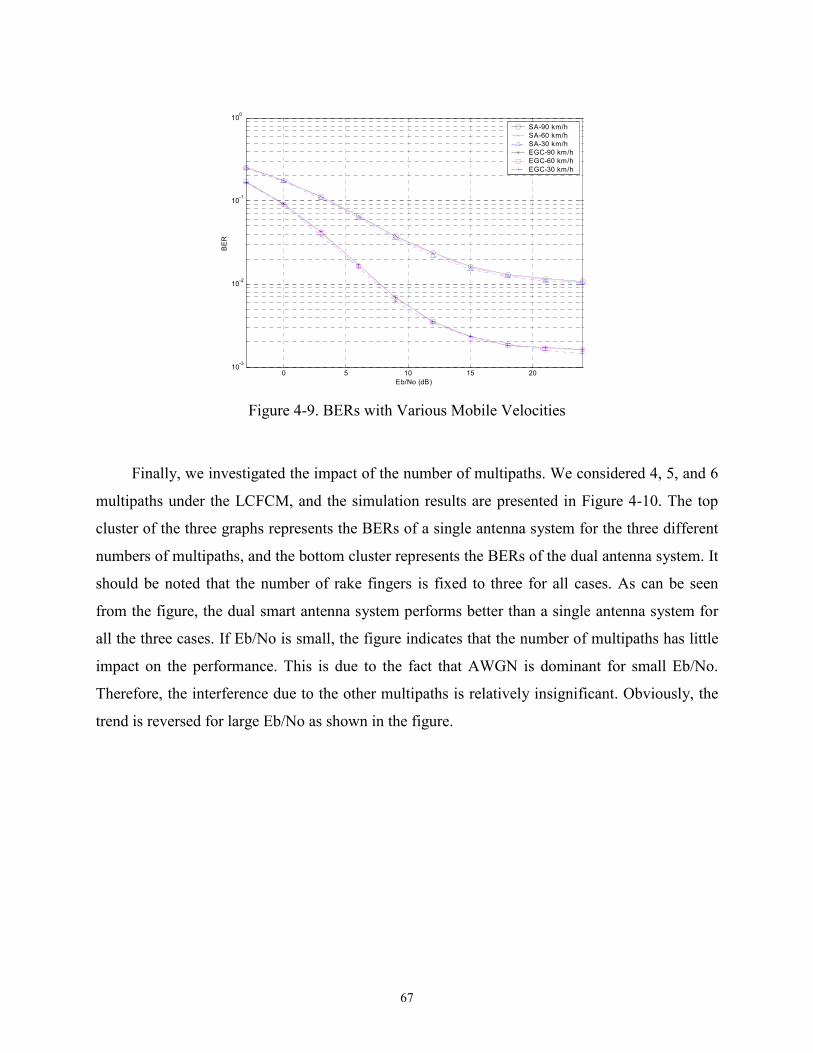
67
0 5 10 15 2010-3
10-2
10-1
100
Eb/No (dB)
BE
R
SA-90 km/hSA-60 km/hSA-30 km/hEGC-90 km/hEGC-60 km/hEGC-30 km/h
Figure 4-9. BERs with Various Mobile Velocities
Finally, we investigated the impact of the number of multipaths. We considered 4, 5, and 6
multipaths under the LCFCM, and the simulation results are presented in Figure 4-10. The top
cluster of the three graphs represents the BERs of a single antenna system for the three different
numbers of multipaths, and the bottom cluster represents the BERs of the dual antenna system. It
should be noted that the number of rake fingers is fixed to three for all cases. As can be seen
from the figure, the dual smart antenna system performs better than a single antenna system for
all the three cases. If Eb/No is small, the figure indicates that the number of multipaths has little
impact on the performance. This is due to the fact that AWGN is dominant for small Eb/No.
Therefore, the interference due to the other multipaths is relatively insignificant. Obviously, the
trend is reversed for large Eb/No as shown in the figure.
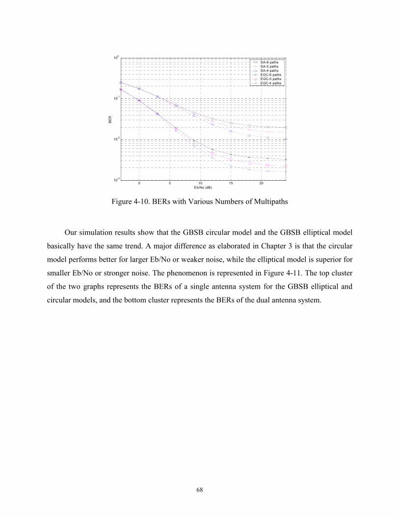
68
0 5 10 15 2010-3
10-2
10-1
100
Eb/No (dB)
BE
R
SA-6 pathsSA-5 pathsSA-4 pathsEGC-6 pathsEGC-5 pathsEGC-4 paths
Figure 4-10. BERs with Various Numbers of Multipaths
Our simulation results show that the GBSB circular model and the GBSB elliptical model
basically have the same trend. A major difference as elaborated in Chapter 3 is that the circular
model performs better for larger Eb/No or weaker noise, while the elliptical model is superior for
smaller Eb/No or stronger noise. The phenomenon is represented in Figure 4-11. The top cluster
of the two graphs represents the BERs of a single antenna system for the GBSB elliptical and
circular models, and the bottom cluster represents the BERs of the dual antenna system.
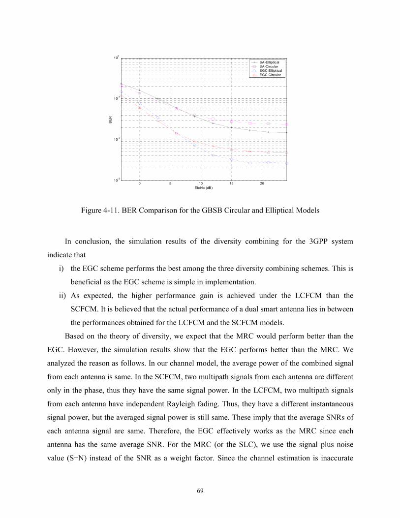
69
0 5 10 15 2010-3
10-2
10-1
100
Eb/No (dB)
BE
R
SA-EllipticalSA-CircularEGC-EllipticalEGC-Circular
Figure 4-11. BER Comparison for the GBSB Circular and Elliptical Models
In conclusion, the simulation results of the diversity combining for the 3GPP system
indicate that
i) the EGC scheme performs the best among the three diversity combining schemes. This is
beneficial as the EGC scheme is simple in implementation.
ii) As expected, the higher performance gain is achieved under the LCFCM than the
SCFCM. It is believed that the actual performance of a dual smart antenna lies in between
the performances obtained for the LCFCM and the SCFCM models.
Based on the theory of diversity, we expect that the MRC would perform better than the
EGC. However, the simulation results show that the EGC performs better than the MRC. We
analyzed the reason as follows. In our channel model, the average power of the combined signal
from each antenna is same. In the SCFCM, two multipath signals from each antenna are different
only in the phase, thus they have the same signal power. In the LCFCM, two multipath signals
from each antenna have independent Rayleigh fading. Thus, they have a different instantaneous
signal power, but the averaged signal power is still same. These imply that the average SNRs of
each antenna signal are same. Therefore, the EGC effectively works as the MRC since each
antenna has the same average SNR. For the MRC (or the SLC), we use the signal plus noise
value (S+N) instead of the SNR as a weight factor. Since the channel estimation is inaccurate

70
due to the noise, the diversity combining with a (S+N) weight factor might not meet the
theoretical expectation. Thus, the performance of the MRC is inferior to that of the EGC. As
shown in [19], there is an imbalance between the average signal powers of dual antennas under
the real environment. In the real environment, the MRC would perform better than the EGC.
The following simple results indicate that the MRC with a SNR weight factor performs better
than the EGC if the average SNR ratio of two antenna signals is two to one, as shown in Table
4-1.
Table 4-1. Performance Comparison of the EGC and the MRC
SNR of Antenna 1
Antenna 1 Antenna 2 EGC MRC with (S+N)
MRC with SNR
-15 dB 18.6 % 26.4 % 14.9 % 15.9 % 13.5 %
-13 dB 11.3 % 18.1 % 7.2 % 8.0 % 6.4 %
-11 dB 4.5 % 8.0 % 1.6 % 2.1 % 1.5 %
4.2 Performance of Adaptive Combining for the 3GPP System
Simulation results to evaluate the performance of the dual smart antenna handsets with the
adaptive combining scheme for the 3GPP system are presented in this section. An adaptive
combiner combines corresponding finger outputs of the two antennas with appropriate antenna
weights, which are recursively obtained based on the N-LMS algorithm.
4.2.1 Simulation Environment
Each antenna receives not only the transmitted signal from the desired base station but also
the transmitted signals from adjacent base stations. The received signal added with background
noise is shaped back with the same FIR filter. Each rake finger despreads a multipath signal from
each antenna. There are two rake finger outputs for each multipath signal – despread pilot signal
and despread data signal. In a single antenna system, each despread data signal is coherently
combined using the despread pilot signal. In a dual antenna system with the adaptive combining
scheme, each despread data signal from each antenna is weighted with the antenna weight and

71
combined. The antenna weights are adaptively obtained using the N-LMS algorithm described in
Chapter 3. Then the output of each adaptive combiner (AC) is coherently combined using the
adaptively combined pilot signal. In our simulation, the coherently combined output of an
antenna system (both single and dual antenna systems) is hard decided to either 1 or 0, and
compared with the original data bits to evaluate the system performance in terms of BER.
The environment considered in our simulation is almost the same as the baseline
parameters described in Section 4.1. The only difference is as follows. Two multipath signals
from an adjacent base station (which is also assumed to transmit the combined signal of eight
users’ signals and the common pilot signal) and background noise (which results in 25 dB of
Eb/N0) are added at handset antennas.
The two factors that affect the performance of the N-LMS algorithm are the step size and
the number of pilot symbols to be averaged. The step size, µ = 0.3, and the number of pilot
symbols, Q = 3, were chosen through trial and error. The three pilot symbol durations correspond
to 0.2 ms in the real operation.
4.2.2 Simulation Results for the AC
The simulation results for the adaptive combining with the GBSB elliptical and circular
models are presented in Figure 4-12. Figure 4-12 (a) and (b) represent the performances of the
dual antenna system with the channel profiles obtained from the GBSB elliptical and circular
models, respectively. In the figure, the y-axis is the BER and the x-axis is the ratio of the average
power of the first multipath signal of the desired base station to the average power of the first
multipath signal of the adjacent base station. The solid line represents the BER of a single
antenna system. The dotted line represents the BER of a dual antenna system with the adaptive
combining. As can be seen from the figure, the dual antenna system with the adaptive combining
performs better than a single antenna system for the GBSB elliptical and circular models. The
performance gain of the dual antenna system with the adaptive combining over a single antenna
system is 3.3 dB for the GBSB elliptical model at BER = 5x10⁻² and 5.5 dB for the GBSB
circular model.

72
-10 -5 0 5 10 15 20 2510-3
10-2
10-1
100
Signal/Interference (dB)
BE
R
Single AntennaAC with N-LMS
(a) BER with the GBSB Elliptical Model
-10 -5 0 5 10 15 20 2510-3
10-2
10-1
100
Signal/Interference (dB)
BE
R
Single AntennaAC with N-LMS
(b) BER with the GBSB Circular Model
Figure 4-12. BERs with the GBSB Elliptical and Circular Models
We investigated the impact of the mobile velocity on the performance of the dual antenna
system with the adaptive combining. We varied the mobile velocity to 2, 10, 30, 60, 90, and 120
km/hr, which results in 4, 20, 59, 119, 178, and 238 Hz of maximum Doppler frequency,
respectively, with the GBSB circular model. Note that all the other parameters remain the same
as the baseline parameters. The simulation results are given in Figure 4-13. The top cluster of the

73
six graphs represents the BERs of a single antenna system with the six mobile velocities. The
bottom cluster of the six graphs represents the BERs of the dual antenna system. The simulation
results reveal that the dual antenna system performs better than a single antenna system for all
the six mobile velocities. It is notable that the impact of the mobile velocity is insignificant for a
single antenna system. However, as the mobile velocity decreases, the BER of the dual smart
antenna system with the adaptive combining also decreases. As expected, the adaptive
combining based on the N-LMS algorithm adapts the antenna weights well as the mobile
velocity decreases.
-10 -5 0 5 10 15 20 2510-3
10-2
10-1
100
Signal/Interference (dB)
BE
R
SA-v120SA-v90SA-v60SA-v30SA-v10SA-v2AC-v120AC-v90AC-v60AC-v30AC-v10AC-v2
Figure 4-13. BERs with Various Mobile Velocities
The simulation results of the adaptive combining for the 3GPP system indicate that
i) the dual smart antenna system with the adaptive combining performs better than a single
antenna system; its performance gain is 3.3 dB for the GBSB elliptical model at BER =
5x10⁻² and 5.5 dB for the GBSB circular model.
ii) As expected, the higher performance gain is achieved as the mobile velocity decreases.

74
4.3 Performance of Hybrid Combining for the 3GPP System
Simulation results to evaluate the performance of the dual smart antenna handsets with the
proposed hybrid combining scheme for the 3GPP system are presented in this section. The
hybrid combiner (HC) combines the diversity combiner (DC) and the adaptive combiner (AC)
outputs using the MRC. The instantaneous signal plus noise (S+N) value is used to weight each
combiner output instead of its SNR. The ECFCM described in Chapter 3 is applied for the
channel model.
4.3.1 Simulation Environment for the GBSB Models
The environment considered in our simulation is almost the same as the baseline
parameters described in Section 4.1. Some differences and additional parameters are as follows.
The distance and the maximum multipath delay are 4000 m and 61 chips in the GBSB circular
model. The envelope correlation of two Rayleigh fading signals for each multipath in the
ECFCM is chosen to be 0.5. The two handset antennas also receive interference and background
noise signals. Two multipath signals from an adjacent base station, which transmits the
combined signal of eight users’ signals and the common pilot signal, are considered. It is noted
that the average SINR is 7.4 dB (due to multipath interference) when there is no interference
from an adjacent base station or noise. The background noise results in 7.0 dB average SINR
without interference. This is due to the multipath interferences. A rake receiver with four rake
fingers is considered at handsets. The same step size, µ = 0.3, and the same number of pilot
symbols to be averaged to obtain the reference signal, Q = 3, are employed for the N-LMS
algorithm as chosen in Section 4.2.
To show the performance of each combining scheme, the plot of BER versus SINR is
presented. Note that BERs of a plot are uncoded ones. To vary the SINR, the average received
power of interference signals from the adjacent base station is changed. To get the average BER
for a given SINR, a number of simulation runs (a simulation run covers the duration of 4 frames)
are repeated until the estimated BER lies within ±2% of the true value with 99% confidence.
Based on the theory of Monte Carlo simulation, the necessary number of error counts is obtained
as 16588 [75]. If not explicitly specified, the channel profile obtained from the GBSB elliptical
model is used in the simulation.

75
4.3.2 Performances of the DC and the AC for the GBSB Models
First, we present the simulation results of the DC and the AC to compare the performances
of these two combining schemes under different operating conditions. The simulation results
with various antenna distances (λ/8, λ/4, 3λ/8, and λ/2) are shown in Figure 4-14. Note that all
the other parameters are the same as the baseline parameters in the simulation. In the figures, the
first line represents the BER of a single antenna (SA) system, and the remaining lines represent
the BERs of the dual antenna system where the antenna distance is λ/8, λ/4, 3λ/8, and λ/2 from
top to bottom. As the distance of two antennas increases, the dual antenna system achieves
higher performance gain. Since the difference in performance between the antenna distances of
λ/2 and λ/4 is small, the dual antenna system with the antenna distance of λ/4 (3.5 cm) is a good
candidate for the practical implementation of both DC and AC. As can be seen from the figure,
the AC performs better than the DC at the low SINR (i.e., interference-limited) environment.
Meanwhile, the DC performs better than the AC at the high SINR (i.e., noise-limited)
environment. For example, the BER of the DC with the antenna distance of λ/4 is 0.13/0.7x10-2
for a low/high SINR = 0.45/6.6 dB, while the BER of AC is 0.11/0.93x10-2 for the same SINR.
The opposite trend of two combining schemes is one of the reasons to propose the HC.
-1 0 1 2 3 4 5 610-3
10-2
10-1
SINR (dB)
BE
R
SADC-0.125λDC-0.25λDC-0.375λDC-0.5λ
(a) Performance of the DC

76
-1 0 1 2 3 4 5 610-3
10-2
10-1
SINR (dB)
BE
R
SAAC-0.125λAC-0.25λAC-0.375λAC-0.5λ
(b) Performance of the AC
Figure 4-14. Performance of the DC and the AC with Various Antenna Distances
To investigate the impact of the mobile velocity, we simulated with various mobile
velocities. The simulation results with various mobile velocities are shown in Figure 4-15. We
varied the mobile velocity to 2, 30, 60, 90, 120, and 150 km/hr, which results in 4, 59, 119, 178,
238, and 297 Hz of maximum Doppler frequency, respectively. In the figures, the upper cluster
of graphs represents the BERs of a single antenna system with various mobile velocities, and the
lower cluster of graphs represents the BERs of the dual antenna system, where the mobile
velocity decreases from top to bottom for each cluster. As can be seen from the figure, the
performances of a single antenna system and the dual antenna system with the DC are little
affected by varying mobile velocities. However, this does not hold for the AC as apparent in
Figure 4-15 (b), i.e., the performance of the AC degrades as the mobile velocity goes high.
Apparently, the AC is tracking well for a low Doppler frequency, i.e., relatively slow fading of
the desired and interfering signals, but is unable to adapt fast enough for a high mobile velocity.
At a high SINR environment, the AC performs better than the DC for a low mobile velocity (2 or
30 km/h), but it is reversed for a high mobile velocity (faster than 60 km/h). This is another
reason to consider the HC.
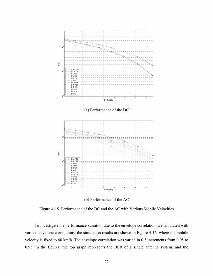
77
-1 0 1 2 3 4 5 610-3
10-2
10-1
SINR (dB)
BE
R
SA-v150SC-v120SA-v90SA-v60SC-v30SA-v2DC-v150DC-v120DC-v90DC-v60DC-v30DC-v2
(a) Performance of the DC
-1 0 1 2 3 4 5 610-3
10-2
10-1
SINR (dB)
BE
R
SA-v150SC-v120SA-v90SA-v60SC-v30SA-v2AC-v150AC-v120AC-v90AC-v60AC-v30AC-v2
(b) Performance of the AC
Figure 4-15. Performance of the DC and the AC with Various Mobile Velocities
To investigate the performance variation due to the envelope correlation, we simulated with
various envelope correlations; the simulation results are shown in Figure 4-16, where the mobile
velocity is fixed to 60 km/h. The envelope correlation was varied in 0.3 increments from 0.05 to
0.95. In the figures, the top graph represents the BER of a single antenna system, and the
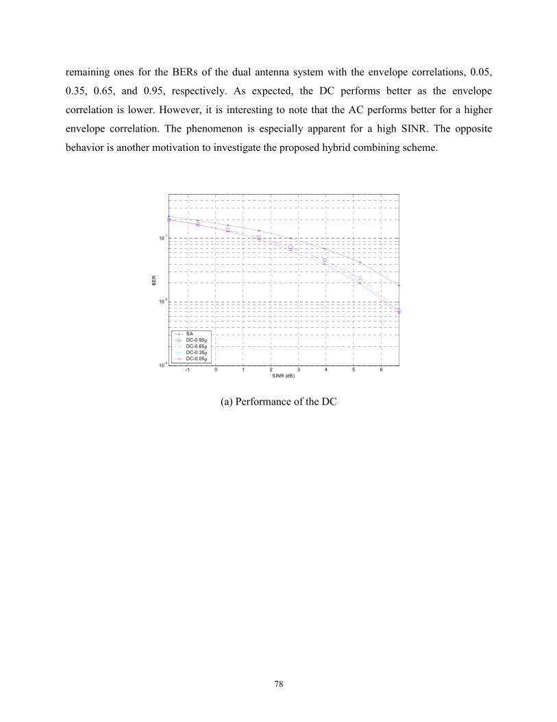
78
remaining ones for the BERs of the dual antenna system with the envelope correlations, 0.05,
0.35, 0.65, and 0.95, respectively. As expected, the DC performs better as the envelope
correlation is lower. However, it is interesting to note that the AC performs better for a higher
envelope correlation. The phenomenon is especially apparent for a high SINR. The opposite
behavior is another motivation to investigate the proposed hybrid combining scheme.
-1 0 1 2 3 4 5 610-3
10-2
10-1
SINR (dB)
BE
R
SADC-0.95ρDC-0.65ρDC-0.35ρDC-0.05ρ
(a) Performance of the DC

79
-1 0 1 2 3 4 5 610-3
10-2
10-1
SINR (dB)
BE
R
SAAC-0.95ρAC-0.65ρAC-0.35ρAC-0.05ρ
(b) Performance of the AC
Figure 4-16. Performance of the DC and the AC with Various Envelope Correlations
The performance trend between the DC and the AC for various envelope correlations is
essentially the same as shown in Figure 4-17 (b), in which the envelope correlation is 0.5. The
only difference is that the cross point (at which they show the same BERs) between the DC and
the AC shifts to the right/left as the envelope correlation increases/decreases.
As noted earlier, two interfering signals from an adjacent base station were considered in
the simulation so far. To investigate the impact of the number of interfering signals from an
adjacent base station, we varied the number of interfering signals from two to four and six in our
simulation. We maintained the total amount of interference power the same in the experiment,
which results in the same SINR for the rake outputs. We observed the same tendency in
performance (which is similar to the one shown in Figure 4-17 (b)). However, a slight decrease
in performance of each combining scheme with an increase of the number of interfering signals
was observed.
Finally, we experimented with the channel profiles obtained from the GBSB circular
model. The simulation results with the GBSB circular model show the same trend as those with
the GBSB elliptical model. The only difference is that the SINR of the rake output (which is
given on the x-axis of a figure) with the GBSB circular model is lower, especially when the same

80
small amount of interferences from an adjacent cell is added. This is due to the effect of
multipaths. The relative distance of a multipath signal to the first multipath signal is smaller for
the GBSB circular model than the GBSB elliptical model. Hence, this results in relatively
smaller path loss, i.e., relatively larger signal power for the multipath signal compared to the
GBSB elliptical model. Since a multipath signal acts as interference to other multipath signals,
strong multipath signal of the circular model results in a strong interference to other multipath
signals. If the interference from an adjacent cell is weak for the circular model, the SINR is
dominant by the multipath interference. Therefore, the SINR of the circular model is smaller than
that of the elliptical model for weak interference from an adjacent cell.
4.3.3 Performance of the HC for the GBSB Models
As observed in Subsection 4.3.2, the DC and the AC exhibit opposite trends in SINR,
mobile velocity, and envelope correlation. Thus, the proposed HC aims to exploit the advantages
of the two combining schemes.
We experimented the performance of the HC for various mobile velocities. As noted
earlier, the AC performs well for a low mobile velocity, while the DC is good for a high velocity.
The simulation results for the mobile velocity of 2 km/hr are shown in Figure 4-17 (a). As can be
seen from the figure, the AC performs the best, while the performance of the HC is equal or
close to that of the AC. When the mobile velocity is increased, the HC performs better than both
the AC and the DC. As a representative case, the simulation results with the mobile velocity of
60 km/hr are shown in Figure 4-17 (b). For instance, the SINR gain of the HC is 0.4 dB higher
than the AC for BER = 0.1 and 0.8 dB higher than the DC. Finally, the DC performs well for a
high mobile velocity. Simulation results for the mobile velocity of 120 km/hr are shown in
Figure 4-17 (c). The figure shows that the performance of the HC is equal to or slightly lower
than that of the DC for the high SINR environment. We observed the same trend for the velocity
of 150 km/hr. In summary, the performance of the HC is better than or equal to the better
performing scheme, either the DC or the AC, for any mobile velocity.
We experimented the HC with various envelope correlations, number of interference
signals, and the GBSB elliptical and circular models. All our observations from the experiments
can be summarized as the performance of the HC is the best or close to the best among the three
schemes.
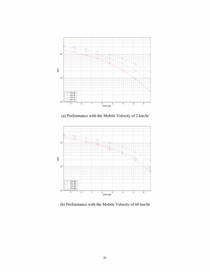
81
-1 0 1 2 3 4 5 610-3
10-2
10-1
SINR (dB)
BE
R
SA-v2DC-v2AC-v2HC-v2
(a) Performance with the Mobile Velocity of 2 km/hr
-1 0 1 2 3 4 5 610-3
10-2
10-1
SINR (dB)
BE
R
SA-v60DC-v60AC-v60HC-v60
(b) Performance with the Mobile Velocity of 60 km/hr
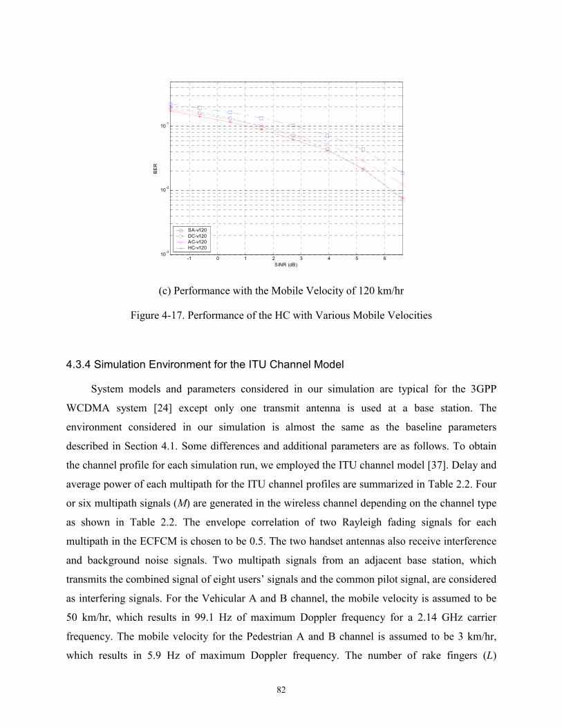
82
-1 0 1 2 3 4 5 610-3
10-2
10-1
SINR (dB)
BE
R
SA-v120DC-v120AC-v120HC-v120
(c) Performance with the Mobile Velocity of 120 km/hr
Figure 4-17. Performance of the HC with Various Mobile Velocities
4.3.4 Simulation Environment for the ITU Channel Model
System models and parameters considered in our simulation are typical for the 3GPP
WCDMA system [24] except only one transmit antenna is used at a base station. The
environment considered in our simulation is almost the same as the baseline parameters
described in Section 4.1. Some differences and additional parameters are as follows. To obtain
the channel profile for each simulation run, we employed the ITU channel model [37]. Delay and
average power of each multipath for the ITU channel profiles are summarized in Table 2.2. Four
or six multipath signals (M) are generated in the wireless channel depending on the channel type
as shown in Table 2.2. The envelope correlation of two Rayleigh fading signals for each
multipath in the ECFCM is chosen to be 0.5. The two handset antennas also receive interference
and background noise signals. Two multipath signals from an adjacent base station, which
transmits the combined signal of eight users’ signals and the common pilot signal, are considered
as interfering signals. For the Vehicular A and B channel, the mobile velocity is assumed to be
50 km/hr, which results in 99.1 Hz of maximum Doppler frequency for a 2.14 GHz carrier
frequency. The mobile velocity for the Pedestrian A and B channel is assumed to be 3 km/hr,
which results in 5.9 Hz of maximum Doppler frequency. The number of rake fingers (L)
83
considered at the receiver for each channel type is also shown in Table 2.2. The same step size,
µ = 0.3 and the same number of pilot symbols to be averaged to obtain the reference signal, Q =
3, are employed for the N-LMS algorithm as chosen in Section 4.2.
4.3.5 The Performance of the DC, the AC, and the HC for the ITU Channel Model
First, we present the simulation results of the DC, the AC, and the HC to compare the
performance of each combining scheme for each channel profile. The simulation results with
each channel profile are shown in Figure 4-18. The simulation results with the ITU Pedestrian A
channel profile are presented in Figure 4-18 (a). In the figures, the square, circle, diamond, and
asterisk lines represent the BERs of a single antenna (SA) system, the DC, the AC, and the HC,
respectively. As can be seen from the figure, the HC performs the best. The AC performs better
than the DC at the low SINR (i.e., interference-limited) environment, while the DC performs
better than the AC at the high SINR (i.e., noise-limited) environment. The SINR gain of the HC
over a single antenna system is 4.28 dB at BER = 10-2 and the SINR gains of the DC and the AC
over a single antenna system are 3.83 dB and 3.58 dB at the same BER, respectively. Figure 4-18
(b) shows the simulation results with the ITU Pedestrian B channel profile. As can be seen from
the figure, the HC performs the best and the DC performs the worst. The performance of the AC
is equal or close to that of the HC.
The simulation results with the Vehicular A channel profile are shown in Figure 4-18 (c).
The HC always performs the best. The AC performs better than the DC at the low SINR
environment, while the DC performs better than the AC at the high SINR environment. The
simulation results with the Vehicular B channel profile show the same trend as that of the
Vehicular A channel profile. The only difference is observed in the combined SINR and the BER
performance, since each channel profile has a different power profile.
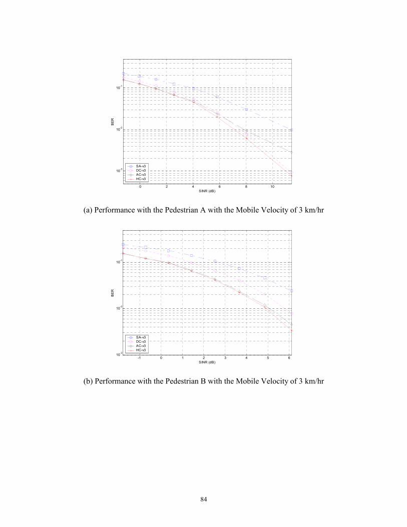
84
0 2 4 6 8 10
10-3
10-2
10-1
SINR (dB)
BE
R
SA-v3DC-v3AC-v3HC-v3
(a) Performance with the Pedestrian A with the Mobile Velocity of 3 km/hr
-1 0 1 2 3 4 5 610-3
10-2
10-1
SINR (dB)
BE
R
SA-v3DC-v3AC-v3HC-v3
(b) Performance with the Pedestrian B with the Mobile Velocity of 3 km/hr

85
-1 0 1 2 3 4 5 610-3
10-2
10-1
SINR (dB)
BE
R
SA-v50DC-v50AC-v50HC-v50
(c) Performance with the Vehicular A with the Mobile Velocity of 50 km/hr
Figure 4-18. Performance of the DC, the AC, and the HC
To investigate the impact of the antenna distance, we simulated with different antenna
distances for the Pedestrian B and the Vehicular A channel profiles. Note that all the other
parameters are the same as the baseline parameters in the simulation. The simulation results of
the HC with various antenna distances (λ/8, λ/4, 3λ/8, and λ/2) for the Pedestrian B channel
profile are shown in Figure 4-19. In the figures, the first line represents the BER of the SA, and
the remaining lines represent the BERs of the dual antenna system where the antenna distance is
λ/8, λ/4, 3λ/8, and λ/2, respectively. The dual antenna system with the antenna distance of 3λ/8
shows the best performance. Since the difference in performance between the antenna distances
of 3λ/8 and λ/4 is small, the dual antenna system with the antenna distance of λ/4 (3.5 cm) is a
good candidate for the practical implementation of the HC. The performance trends of the DC
and the AC are the same as that of the HC. The same trends also hold for the Vehicular A
channel profile.

86
-1 0 1 2 3 4 5 610-3
10-2
10-1
SINR (dB)
BE
R
SAHC-0.125λHC-0.25λHC-0.375λHC-0.5λ
Figure 4-19. Performance of the HC with Various Antenna Distances
To investigate the impact of the mobile velocity, we simulated with various mobile
velocities. The simulation results with various mobile velocities for the Vehicular A channel
profile are shown in Figure 4-20. We varied the mobile velocity to 50, 85, and 120 km/hr, which
results in 99.1, 168.4, and 237.8 Hz of maximum Doppler frequency, respectively. As can be
seen from Figure 4-20 (a), the performances of the dual antenna system with the DC are affected
little by varying mobile velocities. However, this does not hold for the AC as apparent in Figure
4-20 (b), i.e., the performance of the AC degrades as the mobile velocity goes high. Apparently,
the AC is tracking well for a low Doppler frequency, i.e., relatively slow fading of the desired
and interfering signals, but is unable to adapt fast enough for a high mobile velocity. Since the
HC combines the DC and the AC outputs, the performance trend for the HC is the same as that
for the AC.

87
-1 0 1 2 3 4 5 610-3
10-2
10-1
SINR (dB)
BE
R
SADC-v50DC-v85DC-v120
(a) Performance of the DC
-1 0 1 2 3 4 5 610-3
10-2
10-1
SINR (dB)
BE
R
SAAC-v50AC-v85AC-v120
(b) Performance of the AC
Figure 4-20. Performance of the DC and the AC with Various Mobile Velocities
In conclusion, the performance of the proposed hybrid combining scheme is always better
than or equal to those of the adaptive and the diversity combining schemes for all simulation
environments considered.

88
4.4 Performance of Diversity Combining for the cdma2000 System
Simulation results to evaluate the performance of the dual smart antenna handsets with the
diversity combining scheme for the cdma2000 system are presented in this section.
4.4.1 Simulation Environment
The three types of the channel model, LCFCM, SCFCM, and UCFCM, described in
Chapter 3 are employed for the simulation. The signal received at a handset antenna is applied to
its own demodulator and then to a four-finger rake receiver. To process the dual antenna signals,
two levels of diversity combining schemes are considered. The first one is the rake level
diversity combining in which a diversity combiner combines rake receiver outputs. The second
one is the finger level diversity combining in which a diversity combiner combines finger
outputs. Three diversity combining schemes—SD, EGC, and SLC—are considered for each level
(the rake level and the finger level) of diversity combining scheme.
We assumed that the distance from the base station to the mobile station is 1000 m. We
also assumed that the mobile velocity is 100 km/hr, which results in 185 Hz of maximum
Doppler frequency for a 2.0 GHz carrier frequency. In simulating the system with the SPW of
Cadence, we used the link budget shown in Table 4-2. From Table 4-2, only 2.5% (or 0.74 W) of
the total transmitted power of 30 W is allocated to the desired user traffic channel. For the
channel profile, the ITU Vehicular A channel model is applied. A proper level of AWGNs is
added to the channel to achieve 9.75 dB of the signal-to-noise ratio (Eb/N0) on the desired user
traffic channel for the six multipath signals.

89
Table 4-2. Link Budget
Channel Power (W)
Pilot 5.99
Paging 1.89
Sync 0.75
User traffic 0.74
Power control 0.13
Other users 20.50
Total 30.00
The simulation was performed for 3999 frames in which the period of each frame is 20 ms.
Hence, it covers 80 seconds of the real operation. To evaluate the system performance, three
system performance metrics were calculated as described next. After receiving a frame of data,
the transmitted data rate is determined based on the CRC bits and the error metric from the
Viterbi decoder. If the determined data rate is incorrect, a data rate decision error (DRDE)
occurred for the frame. In such a case, a large number of bits are usually erroneous. We assume
that 40% of bits of a frame are in error if a DRDE occurred in the frame. The data rate decision
error rate (DER) is the ratio of the number of DRDE frames to the total number of transmitted
frames (which is 3999). A frame is erroneous if a DRDE occurred and/or at least one bit in the
frame is erroneous. The frame error rate (FER) is the number of erroneous frames to the total
number of frames. A bit error occurs if the received bit does not match the transmitted data bit.
The bit error rate (BER) is the ratio of the number of bit errors to the total number of transmitted
data bits.
4.4.2 Simulation Results
We performed simulation on a Sun UltraSPARC10 workstation with 1 GB of main
memory. The CPU time was not measured, but the elapsed time for the simulation is about six
days for each simulation run. We performed the simulation three times for each type of the
channel model. Then the three simulation results are averaged. In Table 4-3, the simulation
results with three types of the channel model, two levels of diversity combining, and three

90
diversity combining schemes are summarized. The first two rows represent the performance of a
single antenna, while the remaining five rows represent the performance of the dual antennas
with different diversity combining schemes and different level of diversity combining. Two
elements of each entry are the average number of frames out of 3999 frames simulated and its
percentile, respectively. Since each EGC scheme for the rake level and the finger level has the
same operation except for its order, their results are the same. Thus, the only one result is
presented in the table.
When a single antenna is employed, the DERs and the FERs are about the same, with both
measuring around 8%. Since a DRDE always causes a frame error, it can be concluded that most
frame errors are due to DRDEs. When dual antennas are employed, the FERs are reduced to
below 1% for all diversity combining schemes under the UCFCM. However, as the correlation of
dual antenna signals increases from the UCFCM to the SCFCM, the FERs increase up to 6%.
The results also indicate that i) diversity combining scheme at the finger level performs slightly
better than the rake level diversity combining scheme, and ii) EGC scheme performs the best
among the three diversity combining schemes. When EGC scheme is employed for the diversity
combining, the average reduction ratio of the FER for the dual antenna system over the single
antenna system is 13.0 dB (8.65% to 0.43%) for the UCFCM, 2.49 dB (7.98% to 4.50%) for the
LCFCM, and 1.87 dB (8.51% to 5.53%) for the SCFCM. In conclusion, a smart antenna at
handsets significantly improves the performance for the UCFCM, but the improvement is
moderate for the other two channel models.

91
Table 4-3. Performance of Dual Smart Antennas
UCFCM LCFCM SCFCM Scheme Level
DER FER BER DER FER BER DER FER BER
Antenna 1 354.3
8.86%
355.3
8.89% 3.55%
315.7
7.89%
316.0
7.90% 3.16%
343.0
8.58%
344.3
8.61% 3.44%
Antenna 2 335.3
8.39%
336.3
8.41% 3.36%
321.0
8.03%
322.0
8.05% 3.22%
336.0
8.40%
336.7
8.42% 3.36%
Rake 21.7
0.54%
22.0
0.55% 0.22%
200.0
5.00%
200.3
5.01% 2.00%
240.0
6.00%
240.3
6.01% 2.40%SD
Finger 18.3
0.46%
18.7
0.47% 0.19%
193.3
4.83%
193.7
4.84% 1.93%
233.7
5.85%
235.7
5.89% 2.35%
Rake 17.3
0.43%
17.3
0.43% 0.17%
186.0
4.65%
187.3
4.68% 1.88%
226.0
5.65%
226.7
5.67% 2.27%SLC
Finger 16.3
0.41%
16.3
0.41% 0.16%
183.3
4.58%
184.0
4.60% 1.84%
224.0
5.60%
225.7
5.64% 2.26%
Rake EGC
Finger
17.0
0.43%
17.0
0.43% 0.17%
179.7
4.49%
180.0
4.50% 1.80%
220.0
5.50%
221.0
5.53% 2.21%
4.5 Performance of Adaptive Combining for the cdma2000 System
To validate the performance gain of the dual smart antennas at handsets under the
employment of the N-LMS algorithm, the cdma2000 system with the smart antenna is modeled
and simulated with the SPW tool.
4.5.1 Simulation Environment
The signal received at a handset antenna is applied to its own demodulator and then to each
rake finger. In a single antenna system, each rake finger output is coherently combined. In a dual
antenna system with the adaptive combining scheme, each rake finger signal from each antenna
is combined with the adaptively computed antenna weights. Then the output of each adaptive
combiner is coherently combined. The rake finger is a basic building block for a rake receiver,
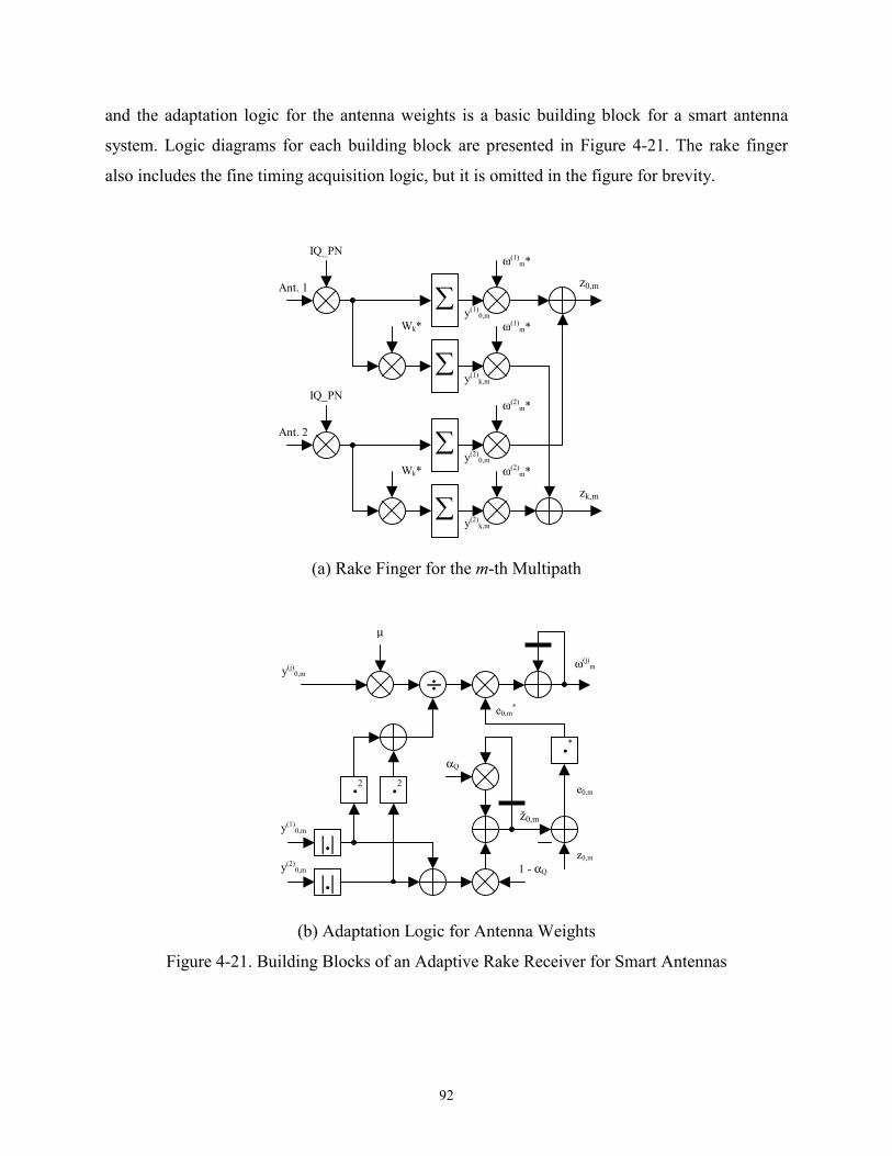
92
and the adaptation logic for the antenna weights is a basic building block for a smart antenna
system. Logic diagrams for each building block are presented in Figure 4-21. The rake finger
also includes the fine timing acquisition logic, but it is omitted in the figure for brevity.
(a) Rake Finger for the m-th Multipath
(b) Adaptation Logic for Antenna Weights
Figure 4-21. Building Blocks of an Adaptive Rake Receiver for Smart Antennas
∑
IQ_PN
Wk* y(1)
0,m
y(1)k,m
ω(1)m*
ω(1)m*
Ant. 1
∑
IQ_PN
Wk* y(2)
0,m
y(2)k,m
ω(2)m*
ω(2)m*
Ant. 2
z0,m
zk,m ∑
∑
y(1)0,m
y(2)0,m
÷y(j)
0,m
µ
ž0,m
z0,m
e0,m
ω(j)m
.*
e0,m*
1 - αQ
αQ
.2.2
|.|
|.|

93
We considered the following environment: the distance from the base station to the mobile
station is 1000 m, and the standard deviation of the path loss in the lognormal fading is 10 dB,
which is a typical value for outdoor channel. In simulating the system with the SPW of Cadence,
we used the same link budget shown in Table 4-2. To shorten the simulation time, a simplified
simulation model was used in our simulation. The number of multipath signals was limited to
two in the channel model. Consequently, a rake receiver with two rake fingers for each antenna
was used to despread and combine the multipath signals. For simplicity, two multipath signals
were assumed to have, on average, the same level of the received signal power. One multipath
signal is effectively an interference signal to the other multipath signal. AWGN is also added to
the channel, and it results in 9.79 dB of SINR. To obtain the reference signal ž0,m(n) in the N-
LMS algorithm, the following infinite impulse response (IIR) method is used for the cdma2000
system instead of the finite impulse response (FIR) method for the 3GPP WCDMA system.
ž0,m(n) =αQ ž0,m(n -1) + (1-αQ)(|y(1)0,m(n)| + |y(2)
0,m(n)|), (4-1)
where αQ is the forgetting factor. The forgetting factor is used to define the relative portion of the
previous pilot symbols to obtain the reference signal. The two factors that affect the performance
of the N-LMS algorithm are the step size and the forgetting factor. The step size, µ = 0.125, and
the two forgetting factors, αQ = 0.975 and 0.9875, were chosen through trial and error.
4.5.2 Simulation Results
We performed the simulation three times for each mobile velocity and each angle of
arrival, in which one simulation run covers 3999 frames. Then the three simulation results are
averaged. The simulation results with different mobile velocity and different angle of arrival are
summarized in Table 4-4. Three different mobile velocities—100 km/h, 50 km/h, and 25 km/h—
were considered, and the maximum Doppler frequencies for the three mobile velocities are 185
Hz, 93 Hz, and 46 Hz for a 2.0 GHz carrier frequency. Two sets of the angle of arrival were
arbitrarily chosen: set 1 (AOA1) with 20° for multipath 1 and 45° for multipath 2, and set 2
(AOA2) with -45° for multipath 1 and 35° for multipath 2. The first two rows in the table
represent the performance of a single antenna. The remaining two rows represent the
performance of the dual antennas with the two different forgetting factors. The top element of
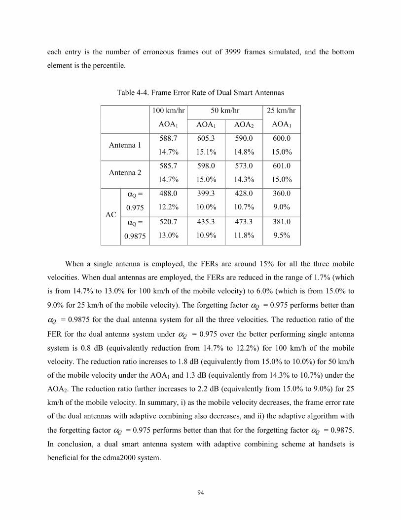
94
each entry is the number of erroneous frames out of 3999 frames simulated, and the bottom
element is the percentile.
Table 4-4. Frame Error Rate of Dual Smart Antennas
50 km/hr 100 km/hr
AOA1 AOA1 AOA2
25 km/hr
AOA1
Antenna 1 588.7
14.7%
605.3
15.1%
590.0
14.8%
600.0
15.0%
Antenna 2 585.7
14.7%
598.0
15.0%
573.0
14.3%
601.0
15.0%
αQ =
0.975
488.0
12.2%
399.3
10.0%
428.0
10.7%
360.0
9.0% AC
αQ =
0.9875
520.7
13.0%
435.3
10.9%
473.3
11.8%
381.0
9.5%
When a single antenna is employed, the FERs are around 15% for all the three mobile
velocities. When dual antennas are employed, the FERs are reduced in the range of 1.7% (which
is from 14.7% to 13.0% for 100 km/h of the mobile velocity) to 6.0% (which is from 15.0% to
9.0% for 25 km/h of the mobile velocity). The forgetting factor αQ = 0.975 performs better than
αQ = 0.9875 for the dual antenna system for all the three velocities. The reduction ratio of the
FER for the dual antenna system under αQ = 0.975 over the better performing single antenna
system is 0.8 dB (equivalently reduction from 14.7% to 12.2%) for 100 km/h of the mobile
velocity. The reduction ratio increases to 1.8 dB (equivalently from 15.0% to 10.0%) for 50 km/h
of the mobile velocity under the AOA1 and 1.3 dB (equivalently from 14.3% to 10.7%) under the
AOA2. The reduction ratio further increases to 2.2 dB (equivalently from 15.0% to 9.0%) for 25
km/h of the mobile velocity. In summary, i) as the mobile velocity decreases, the frame error rate
of the dual antennas with adaptive combining also decreases, and ii) the adaptive algorithm with
the forgetting factor αQ = 0.975 performs better than that for the forgetting factor αQ = 0.9875.
In conclusion, a dual smart antenna system with adaptive combining scheme at handsets is
beneficial for the cdma2000 system.

95
4.6 Summary
In this chapter, we presented the simulation results to evaluate the performance of the
proposed dual smart antenna system at handsets for the 3G wireless personal communication
systems. Simulation results for the 3GPP WCDMA system with diversity combining, adaptive
combining, and hybrid combining schemes were presented in Section 4.1, Section 4.2, and
Section 4.3, respectively. Then, simulation results for the cdma2000 system with diversity
combining and adaptive combining were presented in Section 4.4 and Section 4.5, respectively.
All simulation results indicate that a dual smart antenna system at handsets is effective in
spite of the proximity of the two antennas and the proposed system is beneficial for the 3G
wideband CDMA systems.

96
Chapter 5 Performance of MS-GSC and Adaptive Rake Combining Scheme
In this chapter, we present the simulation results to verify the proposed minimum selection
GSC method and an adaptive rake combining scheme to reduce power dissipation by a mobile
rake receiver. To verify the validity of the proposed adaptive scheme, four rake combining
schemes are applied to a mobile rake receiver for the WCDMA system.
5.1 Simulation Environment
System models and parameters considered in the simulation which results are presented in
this chapter are typical for the 3GPP WCDMA system [24] except only one transmit antenna is
used at a base station. Eight users’ signals with a spreading factor 32 and the common pilot
channel (CPICH) signal with a spreading factor 256 are modulated, channelized, combined,
scrambled, pulse-shaped, and transmitted through the channel. Twenty percent of the total
transmitted power is allocated to the CPICH, and the remaining 80% of the power is allocated
equally to each user signal. For the channel profile (such as delay and average power), the ITU
channel profiles described in [37] are applied.
Delay and average power of each multipath for the ITU channel profiles are summarized in
Table 2.2. Four or six multipath signals (M) are generated in the wireless channel depending on
the channel type as shown in Table 2.2. Each multipath signal is experienced an independent
Rayleigh fading. For the Vehicular A and B channel profiles, the mobile velocity is assumed to
be 50 km/hr, which results in 99.1 Hz of maximum Doppler frequency for a 2.14 GHz carrier

97
frequency. The mobile velocity for the Pedestrian A and B channel profiles is assumed to be 3
km/hr, which results in 5.9 Hz of maximum Doppler frequency. The despread CPICH signal of
each multipath signal is utilized to estimate the channel condition, i.e., the amplitude and the
phase, and thus is used as a weighting factor of each rake finger to combine the selected rake
finger outputs. To reduce the simulation time, channel encoding and decoding is not included.
Thus, a hard decision is made at the output of rake combiner and the output is compared with the
original data bits to evaluate the BER performance. This BER is fed back to the control logic for
the proposed adaptive rake combiners.
5.2 Performance of GSCs: GSC, MS-GSC, AT-GSC, and NT-GSC
First, we present the BER performances of the original GSC, the MS-GSC, the AT-GSC,
and the NT-GSC. Figure 5-1 (a) shows the BER performance of the GSC with five rake fingers
under the ITU Pedestrian B channel profile. GSC (m, 5) performs better as m increases. Figure
5-1 (b) shows the BER performance of the proposed MS-GSC with a threshold set of δ = 0.5. As
shown in the figure, the MS-GSC (Tm, 5) performs better as the threshold Tm becomes larger. The
performance of the MS-GSC is lower and upper bounded by the SC and the MRC, respectively.
The AT-GSC and the NT-GSC show almost the same BER performance as that of the MS-GSC
with a threshold set of δ = 0.5.
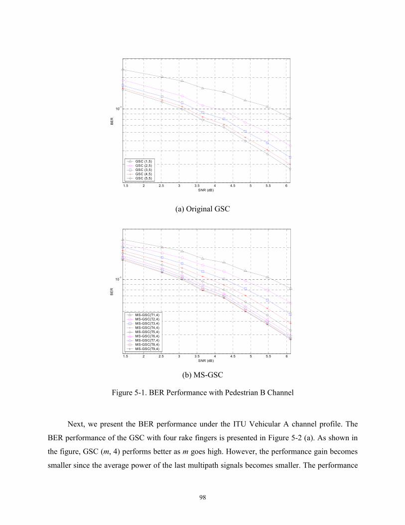
98
1.5 2 2.5 3 3.5 4 4.5 5 5.5 6
10-1
SNR (dB)
BE
R
GSC (1,5)GSC (2,5)GSC (3,5)GSC (4,5)GSC (5,5)
(a) Original GSC
1.5 2 2.5 3 3.5 4 4.5 5 5.5 6
10-1
SNR (dB)
BE
R
MS-GSC(T1,4)MS-GSC(T2,4)MS-GSC(T3,4)MS-GSC(T4,4)MS-GSC(T5,4)MS-GSC(T6,4)MS-GSC(T7,4)MS-GSC(T8,4)MS-GSC(T9,4)
(b) MS-GSC
Figure 5-1. BER Performance with Pedestrian B Channel
Next, we present the BER performance under the ITU Vehicular A channel profile. The
BER performance of the GSC with four rake fingers is presented in Figure 5-2 (a). As shown in
the figure, GSC (m, 4) performs better as m goes high. However, the performance gain becomes
smaller since the average power of the last multipath signals becomes smaller. The performance

99
gain of GSC (3, 4) over GSC (4, 4) is noticeably small. The BER performance of the AT-GSC
with a threshold set of δ = 0.5 is presented in Figure 5-2 (b). As shown in the figure, the AT-
GSC (Ta, 4) performs better as the threshold Ta becomes smaller. The performance of the AT-
GSC is lower and upper bounded by the SC and the MRC, respectively. We observed that the
MS-GSC with a threshold set of δ = 0.5 shows almost the same BER performance as that of the
AT-GSC. The BER performance of the NT-GSC with a threshold set of δ = 0.5 is shown in
Figure 5-2 (c). As shown in the figure, the NT-GSC performs better than the AT-GSC and the
MS-GSC using a threshold set such that the average number of rake fingers activated is the
same. When the Vehicular B channel profile is applied, each generalized selection combining
method (GSC, MS-GSC, AT-GSC, and NT-GSC) shows the same trend as for the case of the
Vehicular A channel profile. The only difference lies in the combined SNR and the BER
performance, since each channel profile has a different power profile.
2 2.5 3 3.5 4 4.5 5 5.5 6 6.510-2
10-1
SNR (dB)
Unc
oded
BE
R
GSC (1,4)GSC (2,4)GSC (3,4)GSC (4,4)
(a) Original GSC

100
2 2.5 3 3.5 4 4.5 5 5.5 6 6.510-2
10-1
SNR (dB)
Unc
oded
BE
R
AT-GSC(T1,4)AT-GSC(T2,4)AT-GSC(T3,4)AT-GSC(T4,4)AT-GSC(T5,4)AT-GSC(T6,4)AT-GSC(T7,4)
(b) AT-GSC
2 2.5 3 3.5 4 4.5 5 5.5 6 6.510-2
10-1
SNR (dB)
Unc
oded
BE
R
NT-GSC(T1,4)NT-GSC(T2,4)NT-GSC(T3,4)NT-GSC(T4,4)NT-GSC(T5,4)NT-GSC(T6,4)NT-GSC(T7,4)
(c) NT-GSC
Figure 5-2. BER Performance with Vehicular A Channel
When the Pedestrian A channel profile is applied with two rake fingers, our simulation
results indicate that the performance difference between GSC (1, 2) and GSC (2, 2) is negligible.
Since the first multipath signal is strong, it results in a large amount of interference for the
second multipath signal (for user data). This interference also results in an imperfect channel
estimation when the second rake finger processes a multipath signal (for the CPICH). Thus, the

101
contribution of the second multipath signal is small or negligible. Therefore, in the following,
only the Pedestrian B and the Vehicular A channel profiles are applied to evaluate the
performance of the proposed adaptive rake combiners.
5.3 Performance of Adaptive Rake Combiners
The BER performance as well as the power reduction of the adaptive rake combining
scheme proposed in Chapter 3 are presented in this section. To generate the feedback
information for the outer loop of the proposed adaptive rake combiners, the current BER
performance is estimated on every frame at the rate of 100 Hz. To adjust the number of rake
fingers activated for the inner loop of the adaptive rake combiner, the combined signal quality is
evaluated in order to check whether it meets the given threshold value provided from the outer
loop at the pilot symbol rate of 15 kHz (= 3.84 MHz / 256). The control logic to evaluate the
BER and the combined signal quality operates at a much lower frequency compared with the
chipping rate (3.84 MHz), at which rake fingers operate. Hence, the power dissipation due to the
control logic would be small when implemented in the CMOS technology. (Note that the power
dissipation is roughly proportional to the operating frequency in the CMOS.) Thus, the power
reduction of the adaptive rake combiner can be represented as the average number of rake fingers
deactivated.
The performance of adaptive rake combiners under various conditions for the ITU
Pedestrian B channel profile with a fixed amount of noise is summarized in Table 5-1. The first
column under "Condition" represents operating conditions, in which the desired target BER and
the average combined SNR with the MRC are presented. A fixed amount of noise is added to the
received signal at the receiver, and we obtain an average combined SNR for five fingers with the
MRC. The relative noise power to the signal power of the first multipath is –12.0 dB, –11.5 dB, -
11.0 dB, and -10.5 dB, which yields 3.66 dB, 4.25 dB, 4.85 dB, and 5.47 dB of the combined
SNR, respectively. The second column under "Performance" has three items such that an average
BER, a normalized standard deviation of the BER (Normal STD), and an average number of rake
fingers deactivated (Finger saving). The normalized standard deviation is computed as the ratio
of standard deviation over the mean of erroneous bits. The column "MRC" represents the
performance of the conventional MRC rake combiner. The last four columns (GSC, MS-GSC,

102
AT-GSC, and NT-GSC) represent the performance of the adaptive rake combiner employing
GSC, MS-GSC, AT-GSC, and NT-GSC, respectively. For brevity, we call them as GSC, MS-
GSC, AT-GSC, and NT-GSC, respectively, in the following.
As presented in Table 5-1, all four GSCs achieve the required BER performance for the
most cases except the AT-GSC under the target BER of 8 %. However, the deviation is less than
1 % (08
08058.
.. − = 0.625 %), which may be insignificant for a channel decoder. The GSC and the
MS-GSC show comparable performance in terms of the average number of fingers deactivated,
and their power reduction due to the deactivated fingers is as high as 52.2 % (= 2.61/4) for the
target BER of 10 %. The AT-GSC and the NT-GSC also show the comparable performance, and
their power reduction is up to 54.0 %. The MS-GSC shows the smallest normalized standard
deviation, which results in the least burst errors. Meanwhile, the AT-GSC shows the largest
normalized standard deviation.

103
Table 5-1. Performance of Adaptive Rake Combiners with Fixed Noise (Pedestrian B)
Condition
Target BER SNR
Performance MRC GSC MS-GSC AT-GSC NT-GSC
BER 8.14 % 9.39 % 9.62 % 9.92 % 9.67 %
Normal STD 32.31 % 25.25 % 19.06 % 33.34 % 26.94 % 3.66 dB
Finger saving 0 1.76 1.67 1.93 1.93
BER 6.42 % 8.56 % 9.16 % 9.10 % 8.91 %
Normal STD 35.05 % 24.46 % 17.10 % 34.50 % 26.13 %
10 %
4.25 dB
Finger saving 0 2.60 2.61 2.64 2.70
BER 6.55 % 7.50 % 7.69 % 8.05 % 7.72 %
Normal STD 36.21 % 29.90 % 22.42 % 38.96 % 31.39 % 4.25 dB
Finger saving 0 1.57 1.56 1.83 1.82
BER 5.05 % 6.80 % 7.29 % 7.35 % 7.11 %
Normal STD 38.67 % 27.52 % 19.79 % 39.85 % 30.05 %
8 %
4.85 dB
Finger saving 0 2.42 2.46 2.52 2.56
BER 5.06% 5.60 % 5.62 % 5.79 % 5.60 %
Normal STD 39.34 % 33.11 % 28.58 % 39.61 % 34.53 % 4.85 dB
Finger saving 0 1.16 1.08 1.23 1.23
BER 3.73 % 4.87 % 5.01 % 5.30 % 5.00 %
Normal STD 44.39 % 32.32 % 24.36 % 47.35 % 36.42 %
6 %
5.47 dB
Finger saving 0 2.08 1.99 2.15 2.20
The simulation results under the ITU Vehicular A channel profile with a fixed amount of
noise are summarized in Table 5-2. The same amount of noise described above for Table 5-1 is
added for the ITU Vehicular A channel profile, which results in 3.90 dB, 4.54 dB, 5.20 dB, and
5.89 dB of the average combined SNR for four fingers with the MRC, respectively. Each
adaptive rake combiner achieves the required BER performance for the most cases except the
AT-GSC under the target BER of 8 %. As in the above case, the deviation is only 0.25 %. The
NT-GSC shows the best performance in terms of power reduction, while the GSC shows the
worst performance. The power reduction with the NT-GSC ranges from 44.5 % (= 1.78/4) to

104
67.8 % (= 2.71/4). As in the case of the Pedestrian B channel profile, the MS-GSC and the AT-
GSC also show the smallest and the largest normalized standard deviation, respectively.
Table 5-2. Performance of Adaptive Rake Combiners with Fixed Noise (Vehicular A)
Condition
Target BER SNR
Performance MRC GSC MS-GSC AT-GSC NT-GSC
BER 8.48 % 9.87 % 9.67 % 9.93 % 9.59 %
Normal STD 22.19 % 26.45 % 21.86 % 27.25 % 25.21 %
3.90 dB
Finger saving 0 1.61 1.88 1.91 2.12
BER 6.63 % 9.58 % 8.98 % 8.96 % 8.76 %
Normal STD 23.48 % 26.06 % 21.58 % 26.57 % 23.95 %
10 %
4.54 dB
Finger saving 0 2.27 2.62 2.54 2.67
BER 6.66 % 7.92 % 7.65 % 8.02 % 7.68 %
Normal STD 23.61 % 29.07 % 22.94 % 29.27 % 27.09 %
4.54 dB
Finger saving 0 1.56 1.84 1.90 2.13
BER 4.89 % 7.69 % 7.05 % 7.05 % 6.87 %
Normal STD 28.27 % 30.73 % 25.93 % 31.87 % 28.95 %
8 %
5.20 dB
Finger saving 0 2.31 2.66 2.58 2.71
BER 4.88 % 5.67 % 5.27 % 5.71 % 5.35 %
Normal STD 27.44 % 36.00 % 26.91 % 35.86 % 31.59 %
5.20 dB
Finger saving 0 1.22 1.39 1.50 1.78
BER 3.41 % 5.67 % 4.97 % 5.15 % 4.94 %
Normal STD 30.13 % 34.41 % 28.57 % 36.88 % 31.89 %
6 %
5.89 dB
Finger saving 0 2.20 2.55 2.48 2.68
To verify the ability of the proposed adaptive rake combiner to dynamically adapt to the
environment, a variable amount of noise is considered for the simulation. A random amount of
noise is added at each simulation run, and 100 runs are performed. The difference between the
maximum and the minimum combined SNRs is about 1.2 dB for 100 runs with a random amount
of noise. The result is almost the same as with a fixed amount of noise. The performance of
adaptive rake combiners under the Pedestrian B and under the Vehicular A channel profiles is
summarized in Table 5-3 and Table 5-4, respectively. As presented in the two tables, each

105
adaptive rake combiner achieves the required BER performance for most cases. With the
exception of a few cases, the maximum deviation is less than 0.5 %. The NT-GSC shows the best
performance in terms of power reduction, in which the maximum power reduction is 65.8 % (=
2.63/4). As in the case of a fixed amount of noise, the MS-GSC and the AT-GSC show the
smallest and the largest normalized standard deviation, respectively.
Table 5-3. Performance of Adaptive Rake Combiners with Variable Noise (Pedestrian B)
Condition
Target BER SNR
Performance MRC GSC MS-GSC AT-GSC NT-GSC
BER 8.31 % 9.49 % 9.76 % 10.01 % 9.75 %
Normal STD 36.35 % 27.86 % 22.60 % 35.28 % 29.69 %
3.66 dB
Finger saving 0 1.70 1.64 1.85 1.86
BER 6.40 % 8.55 % 9.07 % 9.09 % 8.92 %
Normal STD 39.82 % 25.73 % 19.85 % 34.69 % 27.19 %
10 %
4.25 dB
Finger saving 0 2.56 2.51 2.57 2.61
BER 6.43 % 7.51 % 7.81 % 8.02 % 7.77 %
Normal STD 42.89 % 31.38 % 25.42 % 39.54 % 32.81 %
4.25 dB
Finger saving 0 1.69 1.72 1.88 1.88
BER 5.14 % 6.83 % 7.21 % 7.41 % 7.15 %
Normal STD 46.37 % 30.11 % 24.01 % 40.75 % 31.67 %
8 %
4.85 dB
Finger saving 0 2.41 2.39 2.51 2.54
BER 4.99 % 5.67 % 5.71 % 6.03 % 5.78 %
Normal STD 45.48 % 35.97 % 31.64 % 44.67 % 38.11 %
4.85 dB
Finger saving 0 1.45 1.35 1.59 1.58
BER 3.71 % 4.91 % 5.05 % 5.33 % 5.02 %
Normal STD 53.16 % 36.03 % 30.28 % 48.98 % 39.02 %
6 %
5.47 dB
Finger saving 0 2.16 2.10 2.24 2.26
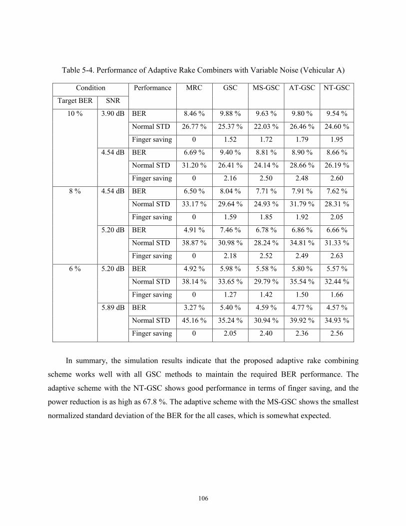
106
Table 5-4. Performance of Adaptive Rake Combiners with Variable Noise (Vehicular A)
Condition
Target BER SNR
Performance MRC GSC MS-GSC AT-GSC NT-GSC
BER 8.46 % 9.88 % 9.63 % 9.80 % 9.54 %
Normal STD 26.77 % 25.37 % 22.03 % 26.46 % 24.60 %
3.90 dB
Finger saving 0 1.52 1.72 1.79 1.95
BER 6.69 % 9.40 % 8.81 % 8.90 % 8.66 %
Normal STD 31.20 % 26.41 % 24.14 % 28.66 % 26.19 %
10 %
4.54 dB
Finger saving 0 2.16 2.50 2.48 2.60
BER 6.50 % 8.04 % 7.71 % 7.91 % 7.62 %
Normal STD 33.17 % 29.64 % 24.93 % 31.79 % 28.31 %
4.54 dB
Finger saving 0 1.59 1.85 1.92 2.05
BER 4.91 % 7.46 % 6.78 % 6.86 % 6.66 %
Normal STD 38.87 % 30.98 % 28.24 % 34.81 % 31.33 %
8 %
5.20 dB
Finger saving 0 2.18 2.52 2.49 2.63
BER 4.92 % 5.98 % 5.58 % 5.80 % 5.57 %
Normal STD 38.14 % 33.65 % 29.79 % 35.54 % 32.44 %
5.20 dB
Finger saving 0 1.27 1.42 1.50 1.66
BER 3.27 % 5.40 % 4.59 % 4.77 % 4.57 %
Normal STD 45.16 % 35.24 % 30.94 % 39.92 % 34.93 %
6 %
5.89 dB
Finger saving 0 2.05 2.40 2.36 2.56
In summary, the simulation results indicate that the proposed adaptive rake combining
scheme works well with all GSC methods to maintain the required BER performance. The
adaptive scheme with the NT-GSC shows good performance in terms of finger saving, and the
power reduction is as high as 67.8 %. The adaptive scheme with the MS-GSC shows the smallest
normalized standard deviation of the BER for the all cases, which is somewhat expected.

107
5.4 Summary
In this chapter, we presented the simulation results to verify the proposed minimum
selection GSC method and an adaptive rake combining scheme to reduce power dissipation by a
mobile rake receiver. To verify the validity of the proposed adaptive scheme, four rake
combining schemes were applied to a mobile rake receiver for the WCDMA system. Simulation
environment considered in the simulations was briefly described in Section 5.1. The BER
performances of the original GSC, the AT-GSC, the NT-GSC, and the proposed MS-GSC were
presented in Section 5.2. Finally, the BER performance as well as the power reduction of the
proposed adaptive rake combining scheme were presented in Section 5.3.
The simulation results indicate that the proposed adaptive rake combining scheme works
well with all GSC methods to maintain the required BER performance. The adaptive scheme
with the MS-GSC shows the smallest normalized standard deviation of the BER for the all cases.
108
Chapter 6 Conclusion
Smart antenna technology is a promising means to overcome signal impairments in
wireless personal communications. When spatial signal processing achieved through smart
antennas is combined with temporal signal processing, the space-time processing can mitigate
interference and multipath to yield higher network capacity, coverage, and quality.
In this dissertation, we propose a dual smart antenna system incorporated into handsets for
the third generation wireless personal communication systems in which the two antennas are
separated by a quarter wavelength (3.5 cm). We examine the effectiveness of a dual smart
antenna system with diversity and adaptive combining schemes and propose a new combining
scheme called hybrid combining. The proposed hybrid combiner combines diversity combiner
and adaptive combiner outputs using maximal ratio combining (MRC). Since these diversity
combining and adaptive combining schemes exhibit somewhat opposite and complementary
characteristics, the proposed hybrid combining scheme aims to exploit the advantages of the two
schemes.
To model dual antenna signals, we consider three channel models: loosely correlated fading
channel model (LCFCM), spatially correlated fading channel model (SCFCM), and envelope
correlated fading channel model (ECFCM). Each antenna signal is assumed to have independent
Rayleigh fading in the LCFCM. In the SCFCM, each antenna signal is subject to the same
Rayleigh fading, but is different in the phase due to a non-zero angle of arrival (AOA). The
LCFCM and the SCFCM are useful to evaluate the upper and the lower bounds of the system
performance. To model the actual channel of dual antenna signals lying in between these two
channel models, the ECFCM is considered. In this model, two Rayleigh fading antenna signals
for each multipath are assumed to have an envelope correlation and a phase difference due to a
non-zero AOA. To obtain the channel profile, we adopt not only the geometrically based single

109
bounce (GBSB) circular and elliptical models, but also the International Telecommunication
Union (ITU) channel model.
The simulation results indicate that the performance of the proposed hybrid combining
scheme is always better than or equal to those of the adaptive and the diversity combining
schemes for all simulation environments considered. For example, the SINR gain of the hybrid
combiner over a single antenna system is 4.28 dB at BER = 10-2 with the ITU Pedestrian A
channel profile. Meanwhile, the SINR gains of the diversity combiner and the adaptive combiner
are 3.83 dB and 3.58 dB at the same condition, respectively.
In this dissertation, we also propose a new generalized selection combining (GSC) method
called minimum selection GSC (MS-GSC) and an adaptive rake combining scheme to reduce the
power consumption of mobile rake receivers. The proposed MS-GSC selects a minimum number
of branches as long as the combined SNR is maintained larger than a given threshold. The
proposed adaptive rake combining scheme which dynamically determines the threshold values is
applicable to the three GSC methods: the absolute threshold GSC, the normalized threshold GSC
(NT-GSC), and the proposed MS-GSC. Through simulation, we estimated the effectiveness of
the proposed scheme for a mobile rake receiver for a wideband CDMA system. We also suggest
a new power control strategy to maximize the benefit of the proposed adaptive scheme. The
simulation results indicate that the proposed adaptive rake combining scheme works well with all
GSC methods to maintain the required BER performance. The adaptive scheme with the NT-
GSC shows good performance in terms of finger saving, and the power reduction is as high as
67.8 %. The adaptive scheme with the MS-GSC shows the smallest normalized standard
deviation for the all cases.
In summary, we investigated the effectiveness of smart antennas at handsets. We proposed
a hybrid combining scheme, a new generalized selection combining scheme, and an adaptive
rake combining scheme, all of which improve the performance of smart antennas at handsets.

110
References
[1] J. Litva and T. K. Lo, Digital Beamforming in Wireless Communications, Artech House,
Massachusetts, 1996.
[2] A. J. Paulraj and B. C. Ng, “Space-Time Modems for Wireless Personal Communications,”
IEEE Personal Communications, pp. 36-48, February 1998.
[3] R. Kohno, “Spatial and Temporal Communication Theory Using Adaptive Antenna Array,”
IEEE Personal Communications, pp. 28-35, February 1998.
[4] J. H. Winters, “Smart Antennas for Wireless Systems,” IEEE Personal Communications,
pp. 23-27, February 1998.
[5] L. C. Godara, “Applications of Antenna Arrays to Mobile Communications, Part I:
Performance Improvement, Feasibility, and System Considerations,” Proceedings of the
IEEE, Vol. 85, No. 7, pp. 1031-1060, July 1997.
[6] L. C. Godara, “Applications of Antenna Arrays to Mobile Communications, Part II: Beam-
Forming and Direction-of-Arrival Considerations,” Proceedings of the IEEE, Vol. 85, No.
8, pp. 1195-1245, August 1997.
[7] A. J. Paulraj and C. B. Papadias, “Space-Time Processing for Wireless Communications,”
IEEE Signal Processing Magazine, pp. 49-83, November 1997.
[8] J. Razavilar, F. Rashid-Farrokhi, and K. J. R. Liu, “Software Radio Architecture with Smart
Antennas: A Tutorial on Algorithms and Complexity,” IEEE Journal of Selected Areas in
Communications, Vol. 17, No. 4, pp. 662-676, April 1999.
[9] J. C. Liberti, Jr. and T. S. Rappaport, Smart Antennas for Wireless Communications: IS-95
and Third Generation CDMA Applications, Prentice Hall, New Jersey, 1999.
[10] W. C. Jakes, Microwave Mobile Communications, John Wiley, New York, 1974.

111
[11] J. S. Thompson, P. M. Grant, and B. Mulgrew, “Smart Antenna Arrays for CDMA
Systems,” IEEE Personal Communications, pp. 16-25, October 1996.
[12] S. Affes and P. Mermelstein, “A New Receiver Structure for Asynchronous CDMA: STAR
– The Spatio-Temporal Array-Receiver,” IEEE Journal on Selected Areas in
Communications, Vol. 16, No. 8, pp. 1411-1422, October 1998.
[13] H. J. Sing, J. R. Crux, and Y. Wang, “Fixed Multibeam Antennas Versus Adaptive Arrays
for CDMA Systems,” IEEE Vehicular Technology Conference, pp. 27-31, September 1999.
[14] M. Dell’Anna and A. H. Aghvami, “Performance of Optimum and Suboptimum Combining
at the Antenna Array of a W-CDMA System,” IEEE Journal of Selected Areas in
Communications, Vol. 17, No. 12, pp. 2123-2137, December 1999.
[15] J. H. Winters, C. C. Martin, and T. Zhuang, “A Two-Element Adaptive Antenna Array for
IS-136 Base Stations,” IEEE Communications Letters, Vol. 3, No. 3, pp. 60-62, March
1999.
[16] C. H. Gowda, V. Annampedu, and R. Viswanathan, “Diversity Combining in Antenna
Array Base Station Receiver for DS/DMA System,” IEEE Communications Letters, Vol. 2,
No. 7, pp. 180-182, July 1998.
[17] A. F. Naguib and A. Paulraj, “Performance of Wireless CDMA with M-ary Orthogonal
Modulation and Cell Site Antenna Arrays,” IEEE Journal of Selected Areas in
Communications, Vol. 14, No. 9, pp. 1770-1783, December 1996.
[18] Y. S. Song and H. M. Kwon, “Analysis of a Simple Smart Antenna for CDMA Wireless
Communications,” IEEE Vehicular Technology Conference, pp. 254-258, May 1999.
[19] C. B. Dietrich, K. Dietze, J. R. Nealy, and W. L. Stutzman, “Spatial, Polarization, and
Pattern Diversity for Wireless Handheld Terminals,” IEEE Transactions on Antennas and
Propagation, Vol. 49, No. 9, pp. 1271-1281, September 2001.
[20] http://www.qualcomm.com/hdr/pdfs/HDR_Tech_Airlink.pdf, “1x High Data Rate
(1xHDR) Airlink Overview,” April 2000.
[21] G. Dolmans and L. Leyten, “Performance Study of an Adaptive Dual Antenna Handset for
Indoor Communications,” IEE Proceedings of Microwaves, Antennas and Propagation,
Vol. 146, No. 2, pp. 138-1444, April 1999.
112
[22] P. B. Wong and D. C. Cox, “Low-Complexity Cochannel Interference Cancellation and
Macroscopic Diversity for High-Capacity,” IEEE Transactions on Vehicular Technology,
Vol. 47, No. 1, pp. 124-132, February 1998.
[23] P. B. Wong and D. C. Cox, “Low-Complexity Diversity Combining Algorithm and Circuit
Architectures for Co-Channel Interference Cancellation and Frequency-Selective Fading
Mitigation,” IEEE Transactions on Communications, Vol. 44, No. 9, pp. 1107-1116,
September 1996.
[24] http://www.3gpp.org/.
[25] H. Holma and A. Toskala, WCDMA for UMTS: Radio Access for Third Generation Mobile
Communications, Wiley, New York, 2000
[26] http://www.3gpp.org/ftp/Specs/2000-12/R1999/25_series/25101-350.zip, “3GPP TS 25.101
UE Radio Transmission and Reception (FDD),” 3GPP, December 2000.
[27] B. O’Hara and A. Petrick, The IEEE 802.11 Handbook: A Designer’s Companion, IEEE
Press, New Jersey, 1999.
[28] S. W. Kim, D. S. Ha, and J. H. Kim, “Performance Gain of Smart Dual Antennas at
Handsets in 3G CDMA System,” The 5th CDMA International Conference, Vol. 2, pp. 223-
227, November 2000.
[29] S. W. Kim, D. S. Ha, and J. H. Kim, “Performance of Smart Antennas with Adaptive
Combining at Handsets for the cdma2000 System,” International Conference on Third
Generation Wireless and Beyond, pp. 882-887, May/June 2001.
[30] S. W. Kim, D. S. Ha, and J. H. Kim, “Performance Gain of Smart Antennas with Diversity
Combining at Handsets for the 3GPP WCDMA System,” The 13th International
Conference on Wireless Communications, pp. 235-242, July 2001.
[31] S. W. Kim, D. S. Ha, J. H. Kim, and J. H. Kim, "Performance Gain of Smart Antennas with
Hybrid Combining at Handsets for the 3GPP WCDMA System," The Fourth International
Symposium on Wireless Personal Multimedia Communications, pp. 289-294, September
2001.
[32] S. W. Kim, D. S. Ha, J. H. Kim, and J. H. Kim, "Performance of Smart Antennas with
Adaptive Combining at Handsets for the 3GPP WCDMA System," The IEEE Vehicular
Technology Conference, pp. 2048-2052, October 2001.

113
[33] R. B. Ertel and J. H. Reed, “Generation of Two Equal Power Correlated Rayleigh Fading
Envelopes,” IEEE Communications Letters, pp. 276-278, October 1998.
[34] R. B. Ertel, P. Cardieri, K. W. Sowerby, T. S. Rappaport, and J. H. Reed, “Overview of
Spatial Channel Models for Antenna Array Communication Systems,” IEEE Personal
Communications, pp. 10-22, February 1998.
[35] R. B. Ertel and J. H. Reed, “Angle and Time of Arrival Statistics for Circular and Elliptical
Scattering Models,” IEEE Journal of Selected Areas in Communications, Vol. 17, No. 11,
pp. 1829-1840, November 1999.
[36] R. B. Ertel, “Antenna Array Systems: Propagation and Performance,” Ph. D. Dissertation,
Department of Electrical and Computer Engineering, Virginia Polytechnic Institute and
State University, July 1999.
[37] ITU ITU-R M.1225, “Guidelines for Evaluations of Radio Transmission Technologies for
IMT-2000,” 1997.
[38] N. Kong, T. Eng, and L. B. Milstein, “A Selection Combining Scheme for RAKE
Receivers,” IEEE International Conference on Universal Personal Communications, pp.
426-430, November 1995.
[39] T. Eng, N. Kong, and L. B. Milstein, “Comparison of Diversity Combining Techniques for
Rayleigh-Fading Channels,” IEEE Transactions on Communications, Vol. 44, No. 9, pp.
1117-1129, September 1996.
[40] N. Kong and L. B. Milstein, “Average SNR of a Generalized Diversity Selection
Combining Scheme,” IEEE Communications Letters, Vol. 3, No. 3, pp. 57-59, March 1999.
[41] N. Kong and L. B. Milstein, “SNR of Generalized Diversity Selection Combining with
Nonidentical Rayleigh Fading Statistics,” IEEE Transactions on Communications, Vol. 48,
No. 8, pp. 1266-1271, August 2000.
[42] M. Z. Win and J. H. Winters, “Virtual Branch Analysis of Symbol Error Probability for
Hybrid Selection/Maximal-Ratio Combining in Rayleigh Fading,” IEEE Transactions on
Communications, Vol. 49, No. 11, pp. 1926-1934, November 2001.
[43] M.-S. Alouini and M. K. Simon, “An MGF-based Performance Analysis of Generalized
Selection Combining over Rayleigh Fading Channels,” IEEE Transactions on
Communications, Vol. 48, No. 3, pp. 401-415, March 2000.

114
[44] M.-S. Alouini and M. K. Simon, “Performance of Coherent Receivers with Hybrid
SC/MRC over Nakagami-m Fading Channels,” IEEE Transactions on Vehicular
Technology, Vol. 48, No. 4, pp. 1155-1164, July 1999.
[45] A. Annamalai and C. Tellambura, “Error Rates for Hybrid SC/MRC Systems on
Nakagami-m Channels,” IEEE Wireless Communications and Networking Conference, pp.
227-231, September 2000.
[46] Y. Ma and C. C. Chai, “Unified Error Probability Analysis for Generalized Selection
Combining in Nakagami Fading Channels,” IEEE Journal on Selected Areas in
Communications, Vol. 18, No. 11, pp. 2198-2210, November 2000.
[47] N. Kong, “Average Signal-to-Interference-plus-Noise Ratio of a Generalized Optimum
Selection Combiner for Non-identical Independent Rayleigh Fading Channels in the
Presence of Co-channel Interference,” IEEE International Conference on Communications,
pp. 990-994, June 2001.
[48] M. Z. Win and J. H. Winters, “Analysis of Hybrid Selection/Maximal-Ratio Combining in
Rayleigh Fading,” IEEE Transactions on Communications, Vol. 47, No. 12, pp. 1773-
1776, December 1999.
[49] J. A. Ritcey and M. Azizoglu, “Performance Analysis of Generalized Selection Combining
with Switching Constraints,” IEEE Communications Letters, Vol. 4, No. 5, pp. 152-154,
May 2000.
[50] C. M. Lo and W. H. Lam, “Approximate BER Performance of Generalized Selection
Combining in Nakagami-m Fading,” IEEE Communications Letters, Vol. 5, No. 6, pp. 254-
256, June 2001.
[51] L. Yue, “Analysis of Generalized Selection Combining Techniques,” IEEE Vehicular
Technology Conference, pp. 1191-1195, May 2000.
[52] A. I. Sulyman and M. Kousa, “Bit Error Rate Performance of a Generalized Diversity
Selection Combining Scheme in Nakagami Fading Channels,” IEEE Wireless
Communications and Networking Conference, pp. 1080-1085, September 2000.
[53] M. K. Simon and M.-S. Alouini, “Performance Analysis of Generalized Selection
Combining with Threshold Test per Branch (T-GSC),” IEEE Global Telecommunications
Conference, pp. 1176-1181, November 2001.
[54] J. G. Proakis, Digital Communications, McGraw-Hill, New York, 1995.

115
[55] S. Haykin, Adaptive Filter Theory, Prentice Hall, New Jersey, 1996.
[56] J. H. Reed, Software Radios: A Modern Approach to Radio Engineering, Prentice Hall,
New Jersey, 2002.
[57] J. H. Winters, “Optimum Combining in Digital Mobile Radio with Cochannel
Interference,” IEEE Transactions on Vehicular Technology, Vol. VT-33, No. 3, pp. 144-
155, August 1984.
[58] J. Salz and J. H. Winters, “Effect of Fading Correlation of Adaptive Arrays in Digital
Mobile Radio,” IEEE Transactions on Vehicular Technology, pp. 1049-1057, November
1994.
[59] S. Tanaka, A. Harada, M. Sawahashi, and F. Adachi, “Experiments on Coherent Adaptive
Antenna Array Diversity for Wideband DS-CDMA Mobile Radio,” IEEE Journal of
Selected Areas in Communications, Vol. 18, No. 8, pp. 1495-1504, August 2000.
[60] S. Tanaka, M. Sawahashi, and F. Adachi, “Pilot Symbol-Assisted Decision-Directed
Coherent Adaptive Array Diversity for DS-CDMA Mobile Radio Reverse Link,” IEICE
Transactions on Fundamentals, Vol. E80-A, No. 12, pp. 2445-2454, December 1997.
[61] R. H. Clarke, “A Statistical Theory of Mobile-Radio Reception,” The Bell System
Technical Journal, Vol. 47, No. 6, pp. 957-1000, July-August 1968.
[62] J. S. Colburn, Y. Rahmat-Samii, M. A. Jensen, and G. J. Pottie, “Evaluation of Personal
Communications Dual-Antenna Handset Diversity Performance,” IEEE Transactions on
Vehicular Technology, Vol. 47, No. 3, pp. 737-746, August 1998.
[63] R. Prasad and T. Ojanpera, “An Overview of CDMA Evolution Toward Wideband
CDMA,” IEEE Communications Surveys, Vol.1, No. 1, pp. 2-29, Fourth Quarter 1998.
[64] L. B. Milstein, “Wideband Code Division Multiple Access,” IEEE Journal of Selected
Areas in Communications, Vol. 18, No. 8, pp. 1344-1354, August 2000.
[65] http://www.cdg.org/frame_3giis.html, “Wideband cdmaOne (TIA cdma2000) Radio
Transmission Technology Proposal,” International Telecommunication Union,
Radiocommunication Study Groups, June 1998.
[66] T. S. Rappaport, Wireless Communications: Principles and Practice, Prentice Hall, New
Jersey, 1996.
[67] http://www.3gpp.org/ftp/tsg_ran/WG1_RL1/TSGR1_18/Docs/PDFs/R1-01-0030.pdf
116
[68] G. Yeap, Practical Low Power Digital VLSI design, Kluwer Academic Publishers,
Massachusetts, 1998.
[69] N. H. Weste and K. Eshraghian, Principles of CMOS VLSI Design: A System Perspective,
Addison Wesley, 1992.
[70] A. P. Chandrakasan, S. Sheng, and R. W. Brodersen, “Low-Power CMOS Digital Design,”
IEEE Journal of Solid-State Circuits, Vol. 27, No. 4, pp. 473-484, April 1992.
[71] A. P. Chandrakasan, M. Potkonjak, R. Mehra, J. Rabaey, and R. W. Brodersen,
“Optimizing Power Using Transformation,” IEEE Transactions on Computer-Aided Design
and Integrated Circuits and Systems, Vol. 14, No. 1, pp. 12-31, January 1995.
[72] A. P. Chandrakasan and R. W. Brodersen, “Minimizing Power Consumption in Digital
CMOS Circuits,” Proceedings of IEEE, Vol. 83, No. 4, pp. 498-523, April 1995.
[73] B. Daneshrad, J. N. Duan, E. Grayver, C. T. Huang, S. W. Kim, and L. J. Ko,
“Parametrizable VLSI Application Specific Datapaths for High Speed Data
Communications,” International Journal of Wireless Information Networks, Vol. 6, No. 4,
pp. 285-301, October 1999.
[74] M. C. Jeruchim, P. Balaban, and K. S. Shanmugan, Simulation of Communication Systems,
Plenum Press, New York, 1994.
[75] S. L. Miller, EE 689: Wireless Communication Systems, Lecture Note, Department of
Electrical Engineering, Texas A&M University, January 2001.

117
Appendix A: Simulation Model for the 3GPP WCDMA System
This appendix describes Matlab codes used for simulating the 3GPP WCDMA system. The
Matlab codes to evaluate the performance of the hybrid combiner and to verify the MS-GSC
method and the adaptive rake combining scheme are presented.
A.1 Matlab Codes for the Hybrid Combiner
There are three parts in the main module for the hybrid combiner (HC). The first part
defines the system and model parameters. A simulation core of the main module constitutes the
second part, in which a number of simulations are run to evaluate the average system
performance. The last part is a post processing, where the BERs are calculated and the
simulation results are saved as a binary file.
A.1.1 System and Model Parameters
The first part of the main module to define the system and model parameters is presented in
Figure A-1. These parameters include the channel model, the Monte Carlo simulation, downlink
signaling, an OVSF code and a scramble code, the common pilot symbol, a pulse shaping FIR
filter, the multiple access interference, receivers, receiving signal, the GBSB model, the ECFCM,
and so forth.
% Channel Model Parameters
ITU_mode = 3; % ITU mode: 1) Pedestrian A, 2) Pedestrian B, 3) Vehicular A, and 4) Vehicular B
rho = 0.50; % Envelope correlation
d = 0.25; % element separation (normalized by wavelength) such as 0.125, 0.25, 0.375, and 0.5
if ITU_mode == 1 | ITU_mode == 2

118
vhr = 3; % velocity of the users (km/h)
else
vhr = 50;
end
CHPF_model = 3; % Channel profile: 1) GBSB Elliptical, 2) GBSB Circular, 3) ITU
channel_model = 4; % channel model selection (1: SCFCM, 2: LCFCM, 3: rho-envelope
correlated, 4: rho-envelope correlated with constant phase difference)
if ITU_mode == 1
L = 4; % # multipaths in the channel
M = 2; % # RAKE fingers (M<=L)
else
L = 6;
if ITU_mode == 2
M = 5;
elseif ITU_mode == 3 | ITU_mode == 4
M = 4;
end
end
% Simulation (Monte Carlo) Parameters
no_iter = 5000; % Maximum number of Iteration
min_no_iter = 50; % Minimum number of iterations
max_error_count = 16745; % Number of errors count for Monte Carlo Simulation
ebno = 10*log10(2); % AWGN with 1/2 power of desired signal power (sum of each
multipath power)
SINR_min = -17;
SINR_max = -10;
SINR_step = 1;
SINR_start = SINR_min;
total_no_iter = no_iter*ones((SINR_max-SINR_min+1)/SINR_step,1);
no_pilot_sym_avg = 1; % Number of pilot symbols to be used to obtain average power
valid_frame = 3; % skip (valid_frame - 1) frames to give the converging time for
adaptive combining (AC with N-LMS)
% This number should be smaller than block_frame if frame is 1.
% Downlink WCDMA signal parameters
K = 8; % # users
des_usr_indx = floor(K/2)+1; % Desired user index
sf_no = 13; % slot format number (0-16) for user's DPCH
s_format = slot_format(sf_no); % returns slot format: s_format(1)=sf, s_format(2)= Ndata1,
s_format(3)= Ndata3, s_format(4)= Ntpc, s_format(5)= Ntfci, s_format(6)= Npilot
sf_index = s_format(1); % spreading factor index
sf_user = sf_index.*ones(K,1); % spreading factor for the users DP(D/C)CH (32 for I and Q)
sf_common = 256; % spreading factor for CCPCH
pri_pilot = 1+j; % P-CPICH (Primary Common Pilot Channel) signal
ovsf_code_numb = floor(linspace(3,sf_index,K))';
block_frame = 4; % # blocks of frames (Total # of frame = block_frame*frame)
frame = 1; % # frames in a block of frames
slot_frame = 15; % # slots per frame
pilot_slot = s_format(6); % # pilot symbols per slot
chip_frame = 38400; % # chips per frame
samp_chip = 4; % # samples per chip

119
% Downlink OVSF and long scrambling codes
load ovsf32all.mat ovsf32all; % Loading OVSF codes with SF 32
ovsf_cpich = ones(1,sf_common);
ovsf_user = ovsf32all(ovsf_code_numb,:); % OVSF codes for each user
load sc_code_dl_32_all.mat sc_code_dl_32_all; % Loading Scrambling codes of n=32
scramb_code = sc_code_dl_32_all(1,:); % Scrambling code for the downlink
scramb_code_user = scramb_code.'*ones(1,frame); % repeating the scrambling code for the frames in
a block
scramb_code_user = scramb_code_user(:);
clear sc_code_dl_32_all ovsf32all;
% Pliot symbols and root-raised cosine pulse-shape filter coefficents
pilot = pilot_table_dl(pilot_slot); % loading pilot bits for a frame from pilot symbol table
load p_shape_coeff.mat b; % loading pulse-shaping filter coefficient
sym_slot = sum(s_format(2:6)); % symbols per slot
d_sym_slot = sum(s_format(2:3)); % user data symbols per slot
c_sym_slot = sum(s_format(4:5)); % control symbols per slot (TPC+TFCI not include Pilot)
sym_frame = slot_frame * sym_slot; % symbols per frame
d_sym_frame = slot_frame * d_sym_slot; % user data symbols per frame
cpich_slot = 20; % P-CPICH symbols per slot
cpich_frame = slot_frame * cpich_slot; % P-CPICH symbols per frame
no_symbol_cpich = sym_slot/cpich_slot; % ratio of the number of user symbols to the number of
P-CPICH symbols
no_symbol_slot = sym_slot/2;
% MAI from adjacent cells
NBS = 1; % # adjacent cells
K1 = 8; % # users
L1 = 2; % # multipaths
load sc_code_dl_4128_all.mat sc_code_dl_4128_all; % Loading Scrambling codes of n=32
scramb_code1 = sc_code_dl_4128_all(1,:); % Scrambling code for the downlink
scramb_code_user1 = scramb_code1.'*ones(1,frame); % repeating the scrambling code
scramb_code_user1 = scramb_code_user1(:);
clear sc_code_dl_4128_all;
ovsf_code_numb1 = (3:K1+2)';
load ovsf32all.mat ovsf32all; % Loading OVSF codes with SF 32
ovsf_user1 = ovsf32all(ovsf_code_numb1,:); % OVSF codes for each user
clear ovsf32all;
theta_bs_LOS1 = (-1)*sign(randn(1))*rand(1)*pi/2; % LOS AOA for uniformly distributed (-90, 90)
P_LOS1 = 1.0; % Power of the LOS components (Relative power
of MAI)
% Receiver parameters
N = 2; % # antenna elements
mu = linspace (0.3, 0.3, M); % multiple step sizes of each multipath for LMS
aQ = 3; % Number of pilot symbols to get the averaged power for LMS
% Channel parameters for the GBSB models
n_scat = 50; % # Scatters
tau_min = 10e-3/chip_frame; % Minimum multipath delay (1 chip period in any frame)
if CHPF_model == 1
tau_max = 20*tau_min; % Maximum relative delay (20 chips for GBSB elliptical (D=800m))
D = 800; % 0.5 mile % Distance (m) of each user from the base station

120
elseif CHPF_model == 2
tau_max = 61*tau_min; % Maximum relative delay for GBSB circular (35, 48, 61, 74, 87,
99 chip for D = 2, 3, 4, 5, 6, 7 km)
D = 4000; % 2.5 mile % Distance (m) of each user from the base station
elseif CHPF_model == 3
tau_max = 99*tau_min; % Maximum relative delay when ITU Vehicular B is applied
D = 7000;
end
% Wireless channel parameters
eta = 3.5; % path loss exponent
fc = 2.14e9; % Carrier frequency of Downlink (2.11 ~ 2.17 GHz)
P_LOS = 1; % Power of the LOS components from the users (normalized to 1W)
rayl_frame = block_frame*frame; % # frames used to generate the rayleigh fading profile
theta_bs_LOS = (-1)*sign(randn(1))*rand(1)*pi/2; % LOS AOA for uniformly distributed (-90, 90)
vsec = vhr*1e3*ones(1,1)/3600; % velocity of the users (m/sec)
c = 3e8; % Speed of propagation (m/sec)
fm = vsec*fc/c; % Maximum Doppler spread (Hz)
theta_v = theta_bs_LOS; % Direction of motion of the mobiles (wrt LOS)
% Received signal at Mobile Station
fs = chip_frame*samp_chip*100; % Sampling rate of the transmitted baseband signal (10ms frame)
max_delay = floor(tau_max*fs); % maximum multipath delay in samples
signal_block = frame*chip_frame*samp_chip; % length of the signal observation window in samples
% Power budget for the common pilot (20%)
K_pilot = floor(K/4);
P_ratio = sqrt(K_pilot)/2;
Other_Power = K_pilot + K - 1;
K_pilot1 = floor(K1/4);
P_ratio1 = sqrt(K_pilot1)/2;
Other_Power1 = K_pilot1 + K1 -1;
% Model parameters for the ECFCM
if channel_model == 3 | channel_model == 4
lamda = find_lamda_from_rho(rho);
L_matrix = [ 1 0; 1/sqrt(2)*lamda*(1+j) sqrt(1-lamda^2)];
end
Figure A-1 System and Model Parameters for the HC
A.1.2 Simulation Core
The second part of the main module is a simulation core, in which simulation is iterated for
a number of times to evaluate the average system performance. Figure A-2 presents the
simulation core for the HC. There are several loops in the simulation core. The most outer loop
specifies the number of iterations. The second outer loop is for different SINRs. The third outer
loop repeats for a number of frames for each simulation run. There are several inner loops in this

121
third outer loop. The first and the second inner loops are to generate the transmitted user signal
and to generate multipath signals for this user signal, respectively. The third and the fourth inner
loops are to generate the transmitted signal from other base station and to generate multipath
signals for this interference signal, respectively. Each multipath signal is despread in the last
inner loop using a rake finger.
for iter = 1:no_iter %% loop 1
theta_bs_LOS = (-1)*sign(randn(1))*rand(1)*pi/2;
if CHPF_model == 1
[tau,theta_bs,P,alpha] = … % GBSB elliptical model
vec_ch_ellip_dl_1(n_scat,L,D,tau_max,tau_min,P_LOS,theta_bs_LOS,eta);
elseif CHPF_model == 2
[tau,theta_bs,P,alpha] = … % GBSB circular model
vec_ch_circ_dl_1(n_scat,L,D,tau_max,tau_min,P_LOS,theta_bs_LOS,eta);
elseif CHPF_model == 3
[tau,theta_bs,P,alpha] = … % ITU channel model
vec_ch_umts_dl_1(n_scat,L,D,tau_max,tau_min,P_LOS,theta_bs_LOS,eta,ITU_mode);
end
tau_samp = round(tau*fs); % multipath delays in chip samples
fd = abs(fm*cos(theta_bs-theta_v)); % doppler spread for each multipath
I = find(fd < 1); % If doppler spread < 1 map it to 1
fd(I) = 1;
P_all = sum(P(1:M));
for SINR = SINR_start:SINR_step:SINR_max %% loop 2
theta_bs_LOS1 = (-1)*sign(randn(1))*rand(1)*pi/2;
P_all_1 = (P_all/(10^(SINR/10))-(Other_Power+10^((-1)*ebno/10))*P_all)/(Other_Power1+1);
% Channel profile for MAI
if CHPF_model == 1
[tau1,theta_bs1,P1,alpha1] = …
vec_ch_ellip_dl_2(n_scat,L1,D,tau_max,tau_min,P_all_1,theta_bs_LOS1,eta);
else
[tau1,theta_bs1,P1,alpha1] = …
vec_ch_circ_dl_2(n_scat,L1,D,tau_max,tau_min,P_all_1,theta_bs_LOS1,eta);
end
tau_samp1 = round(tau1*fs); % multipath delays in chip samples
fd1 = abs(fm*cos(theta_bs1-theta_v)); % doppler spread for each multipath
I1 = find(fd1 < 1); % If doppler spread < 1 map it to 1
fd1(I1) = 1;
w_in_lms(1:N,1:M) = [ones(1,M);zeros(N-1,M)]; % Initialization of weight vectors for LMS
e = zeros(block_frame*frame*slot_frame*cpich_slot/2,M); % Initialization of error for LMS
for frame_count = 1:block_frame %% loop 3
pcpi = (pri_pilot*P_ratio)*scramb_code_user; % Primary Common Pilot Signal
for i = 1:K %% loop 4-1
s = wcdma_signal_sym_dl_1(frame,slot_frame,samp_chip,s_format,ovsf_user(i,:),…
scramb_code,pilot_slot,pilot,b,i,des_usr_indx);
pcpi = s + pcpi;
end %% loop 4-1

122
clear s;
sh_s = p_shape_1(b,pcpi,samp_chip,'sqrtrc','xmittr'); % Pulse-shaping of DPDCH
x_i = zeros(N,max_delay + signal_block); % Initialization of the received signal
for ii = 1:L %% loop 4-2
% User's spatial signature vector, A
if channel_model == 1 % SCFCM
A = channel_vector_dl(theta_bs(ii,1),alpha(ii,1),tau_samp(ii,1),N,d,frame,…
sym_frame/2,sf_user(i,1),samp_chip,fd(ii,1),rayl_frame,size(x_i,2),…
max_delay,ii,L,des_usr_indx,des_usr_indx,frame_count);
elseif channel_model == 2 % LCFCM
A = channel_vector_dl_1(theta_bs(ii,1),alpha(ii,1),tau_samp(ii,1),N,d,frame,…
sym_frame/2,sf_user(i,1),samp_chip,fd(ii,1),rayl_frame,size(x_i,2),…
max_delay,ii,L,des_usr_indx,des_usr_indx,frame_count);
elseif channel_model == 3 % original ECFCM
A = channel_vector_dl_2(theta_bs(ii,1),alpha(ii,1),tau_samp(ii,1),N,d,frame,…
sym_frame/2,sf_user(i,1),samp_chip,fd(ii,1),rayl_frame,size(x_i,2),…
max_delay,ii,L,des_usr_indx,des_usr_indx,frame_count);
elseif channel_model == 4 % ECFCM
A = channel_vector_dl_3(theta_bs(ii,1),alpha(ii,1),tau_samp(ii,1),N,d,frame,…
sym_frame/2,sf_user(i,1),samp_chip,fd(ii,1),rayl_frame,size(x_i,2),…
max_delay,ii,L,des_usr_indx,des_usr_indx,frame_count);
end
S = sig_matrix_1(tau_samp(ii,1),sh_s,size(x_i,2),max_delay); % User's signal vector
for iii = 1:N %% loop 5-1
rcx(iii,:) = A(iii,:).*S;
end %% loop 5-1
x_i = x_i + rcx; % Receiver signal from each multipath
end %% loop 4-2
clear rcx S sh_s;
% MAI gereration
pcpi1 = (pri_pilot*P_ratio1)*scramb_code_user1; % Primary Common Pilot Signal
for i = 1:K1 %% loop 4-3
s1 = wcdma_signal_sym_dl_1(frame,slot_frame,samp_chip,s_format,ovsf_user(i,:),…
scramb_code,pilot_slot,pilot,b,i,des_usr_indx);
pcpi1 = s1 + pcpi1;
end %% loop 4-3
clear s1;
sh_s1 = p_shape_1(b,pcpi1,samp_chip,'sqrtrc','xmittr'); % Pulse-shaping of DPDCH
x_i1 = zeros(N,max_delay + signal_block); % Initialization of the received signal
for ii = 1:L1 %% loop 4-4
% User's spatial signature vector, A
if channel_model == 1 % SCFCM
A1 = channel_vector_dl(theta_bs1(ii,1),alpha1(ii,1),tau_samp1(ii,1),N,d,frame,…
sym_frame/2,sf_user(i,1),samp_chip,fd1(ii,1),rayl_frame,size(x_i,2),…
max_delay,ii,L1,des_usr_indx,des_usr_indx,frame_count);
elseif channel_model == 2 % LCFCM
A1 = channel_vector_dl_1(theta_bs1(ii,1),alpha1(ii,1),tau_samp1(ii,1),N,d,frame,…
sym_frame/2,sf_user(i,1),samp_chip,fd1(ii,1),rayl_frame,size(x_i,2),…
max_delay,ii,L1,des_usr_indx,des_usr_indx,frame_count);
elseif channel_model == 3 % original ECFCM

123
A1 = channel_vector_dl_2(theta_bs1(ii,1),alpha1(ii,1),tau_samp1(ii,1),N,d,frame,…
sym_frame/2,sf_user(i,1),samp_chip,fd1(ii,1),rayl_frame,size(x_i,2),…
max_delay,ii,L1,des_usr_indx,des_usr_indx,frame_count);
elseif channel_model == 4 % ECFCM
A1 = channel_vector_dl_3(theta_bs1(ii,1),alpha1(ii,1),tau_samp1(ii,1),N,d,frame,…
sym_frame/2,sf_user(i,1),samp_chip,fd1(ii,1),rayl_frame,size(x_i,2),…
max_delay,ii,L1,des_usr_indx,des_usr_indx,frame_count);
end
S1 = sig_matrix_1(tau_samp1(ii,1),sh_s1,size(x_i1,2),max_delay);
for iii = 1:N %% loop 5-2
rcx1(iii,:) = A1(iii,:).*S;
end %% loop 5-2
x_i1 = x_i1 + rcx1; % Receiver signal from each multipath
end %% loop 4-4
clear rcx1 S1 sh_s1;
shuffle = floor((size(x_i1,2)-1)*rand(1)); % Make two cells asynchronous
x_i1 = [x_i1(:,shuffle+1:end) x_i1(:,1:shuffle)]; % Shuffle the MAIs
x = x_i + x_i1 + noise_4(sf_user(des_usr_indx),ebno,size(x_i),P,M,Other_Power); % AWGN
clear x_i x_i1;
load user_data.mat user_data; % desired user's DPDCH data symbols
x = p_shape_1(b,x.',samp_chip,'sqrtrc','rcvr'); % SQRT-RC filtering at the receiver
x = x.';
for i = 1:M %% loop 4-5
% Frame Synchronization and Decimation
x_chip = x(:,tau_samp(i,1)+1:samp_chip:end);
x_chip = x_chip(:,1:chip_frame*frame); % proper sizing of the chip samples
% De-scrambling and de-spreading
for ii = 1:N %% loop 5-3
x_chip(ii,:) = x_chip(ii,:).*scramb_code_user'; % De-scrambling
y_I(ii,:) = (reshape(x_chip(ii,:),…
length(ovsf_user(des_usr_indx,:)),…
sym_frame/2*frame).'*ovsf_user(des_usr_indx,:)').'/size(ovsf_user(des_usr_indx,:),…
2); % De-spreading for DPCH
y_P(ii,:) = (reshape(x_chip(ii,:),length(ovsf_cpich), …
cpich_frame/2*frame).'*ovsf_cpich').'/size(ovsf_cpich,2);
end %% loop 5-3
z_finger_1(i,:) = y_I(1,:);
z_pilot_1(i,:) = y_P(1,:);
z_finger_2(i,:) = y_I(2,:);
z_pilot_2(i,:) = y_P(2,:);
% N-LMS weight adaptation
[w_lms, w_end_lms, e] = lms_weight1(mu(i), aQ, alpha(i), N, w_in_lms(:,i), y_P, …
e, pri_pilot, cpich_slot/2, frame_count, frame, slot_frame, i);
w_in_lms(:,i) = w_end_lms;
w1_lms = ones(1, sym_frame/cpich_frame)'*w_lms(1,:);
w2_lms = ones(1, sym_frame/cpich_frame)'*w_lms(2,:);
w1_lms = reshape(w1_lms, 1, size(w1_lms,1)*size(w1_lms,2));
w2_lms = reshape(w2_lms, 1, size(w2_lms,1)*size(w2_lms,2));
z_pilot_lms(i,:) = y_P(1,:).*conj(w_lms(1,:)) + y_P(2,:).*conj(w_lms(2,:));

124
z_finger_lms(i,:) = y_I(1,:).*conj(w1_lms) + y_I(2,:).*conj(w2_lms);
end %% loop 4-5
% Phase rotaion using the known pilot signal
[new_z_fin_1] = phase_rotate_1 (frame, slot_frame, z_finger_1, z_pilot_1, …
s_format, sf_common, pri_pilot); % (Antenna 1)
[new_z_fin_2] = phase_rotate_1 (frame, slot_frame, z_finger_2, z_pilot_2, …
s_format, sf_common, pri_pilot); % (Antenna 2)
[new_z_fin_lms] = phase_rotate (frame, slot_frame, z_finger_lms, z_pilot_lms, …
s_format, sf_common, pri_pilot);
z_all_1 = sum (new_z_fin_1,1); % Combining each multipath signal for antenna 1
z_all_2 = sum (new_z_fin_2,1); % Combining each multipath signal for antenna 2
% Maximal ratio combining (MRC) based on data signal (S+N) after rake combining
z_all_3 = (2./(abs(z_all_1)+(abs(z_all_2)))).*(abs(z_all_1).*z_all_1 + …
abs(z_all_2).*z_all_2);
z_all_4 = sum (new_z_fin_lms,1); % Adaptive combining based on N-LMS
% Hybrid combining of DC and AC outputs using MRC
z_all_5 = (abs(z_all_3).*z_all_3 + abs(z_all_4).*z_all_4);
% Hard decision for data detection of I/Q channel
z_I_1 = sign(real(z_all_1));
z_Q_1 = sign(imag(z_all_1));
z_I_2 = sign(real(z_all_2));
z_Q_2 = sign(imag(z_all_2));
z_I_3 = sign(real(z_all_3));
z_Q_3 = sign(imag(z_all_3));
z_I_4 = sign(real(z_all_4));
z_Q_4 = sign(imag(z_all_4));
z_I_5 = sign(real(z_all_5));
z_Q_5 = sign(imag(z_all_5));
z_I_1 = z_I_1(:); z_Q_1 = z_Q_1(:);
z_I_2 = z_I_2(:); z_Q_2 = z_Q_2(:);
z_I_3 = z_I_3(:); z_Q_3 = z_Q_3(:);
z_I_4 = z_I_4(:); z_Q_4 = z_Q_4(:);
z_I_5 = z_I_5(:); z_Q_5 = z_Q_5(:);
data_out_1 = extract_data (frame, slot_frame, z_I_1, z_Q_1, s_format); % Antenna 1
data_out_2 = extract_data (frame, slot_frame, z_I_2, z_Q_2, s_format); % Antenna 2
data_out_3 = extract_data (frame, slot_frame, z_I_3, z_Q_3, s_format); % DC
data_out_4 = extract_data (frame, slot_frame, z_I_4, z_Q_4, s_format); % AC
data_out_5 = extract_data (frame, slot_frame, z_I_5, z_Q_5, s_format); % HC
% Number of error symbols
%------------------------
Nerror_1(frame_count,1) = length(find(data_out_1 ~= user_data));
Nerror_2(frame_count,1) = length(find(data_out_2 ~= user_data));
Nerror_3(frame_count,1) = length(find(data_out_3 ~= user_data));
Nerror_4(frame_count,1) = length(find(data_out_4 ~= user_data));
Nerror_5(frame_count,1) = length(find(data_out_5 ~= user_data));
end %% loop 3
% Symbol error rate
% Error count before valid frame
sinr_index = (SINR-SINR_min)/SINR_step+1;

125
Ne_I_1(sinr_index,iter) = sum(Nerror_1(1:valid_frame-1),1);
Ne_I_2(sinr_index,iter) = sum(Nerror_2(1:valid_frame-1),1);
Ne_I_3(sinr_index,iter) = sum(Nerror_3(1:valid_frame-1),1);
Ne_I_4(sinr_index,iter) = sum(Nerror_4(1:valid_frame-1),1);
Ne_I_5(sinr_index,iter) = sum(Nerror_5(1:valid_frame-1),1);
% Error count from valid frame
Ne_V_1(sinr_index,iter) = sum(Nerror_1(valid_frame:end),1);
Ne_V_2(sinr_index,iter) = sum(Nerror_2(valid_frame:end),1);
Ne_V_3(sinr_index,iter) = sum(Nerror_3(valid_frame:end),1);
Ne_V_4(sinr_index,iter) = sum(Nerror_4(valid_frame:end),1);
Ne_V_5(sinr_index,iter) = sum(Nerror_5(valid_frame:end),1);
Ne_V_6(sinr_index,iter) = sum(Nerror_6(valid_frame:end),1);
end %% loop 2
% Iterating simulations are stopped when the predefined number of errors is occurred
% It can save the simulation time for lower SINR cases.
if iter >= min_no_iter & SINR_start <= SINR_max
if ( sum(Ne_I_5((SINR_start-SINR_min)/SINR_step+1,:)) + …
sum(Ne_V_5((SINR_start-SINR_min)/SINR_step+1,:)) ) > max_error_count
total_no_iter((SINR_start-SINR_min)/SINR_step+1) = iter; % # iterations for each SINR
SINR_start = SINR_start + SINR_step; % Change the starting value
save total_no_iter_file -ascii total_no_iter;
end
end
end %% loop 1
Figure A-2 Simulation Core for the HC
The simulation core also contains several functions. They include a channel profile
generator, a downlink signal generator, a multipath signal vector generator, a noise generator, a
phase rotator for the coherent combining, and an N-LMS antenna weight generator.
A.1.3 Post Processing
The last part of the main module is presented in Figure A-3, in which the BERs are
calculated and the simulation results are saved as a binary file. It consists of three sub-parts. The
first sub-part is to calculate BERs for each antenna and each combining scheme. The second one
is to define a file name to save the simulation results, while the last one is to save the simulation
results into this file.
% BERs for each antenna and each combining scheme
no_sym_iter = d_sym_frame*frame*block_frame; % Number of frames to be simulated
Ps_av_1 = ((sum(Ne_I_1,2)+sum(Ne_V_1,2))./total_no_iter)/no_sym_iter; % Antenna 1
Ps_av_2 = ((sum(Ne_I_2,2)+sum(Ne_V_2,2))./total_no_iter)/no_sym_iter; % Antenna 2

126
Ps_av_3 = ((sum(Ne_I_3,2)+sum(Ne_V_3,2))./total_no_iter)/no_sym_iter; % DC
Ps_av_4 = ((sum(Ne_I_4,2)+sum(Ne_V_4,2))./total_no_iter)/no_sym_iter; % AC
Ps_av_5 = ((sum(Ne_I_5,2)+sum(Ne_V_5,2))./total_no_iter)/no_sym_iter; % HC
SINR = SINR_min:SINR_step:SINR_max;
% Defene a file name to save the simulation results
sim_mode = 'HC';
if CHPF_model == 1
file_head = 'ell';
elseif CHPF_model == 2
file_head = 'cir';
elseif CHPF_model == 3
if ITU_mode == 1
file_head = 'itu_pa';
elseif ITU_mode == 2
file_head = 'itu_pb';
elseif ITU_mode == 3
file_head = 'itu_va';
elseif ITU_mode == 4
file_head = 'itu_vb';
end
end
if d == 0.125
ant_dis = 'd18';
elseif d == 0.25
ant_dis = 'd14';
elseif d == 0.375
ant_dis = 'd38';
elseif d == 0.5
ant_dis = 'd12';
end
if rho == 0.1
rho_d = 'r01';
elseif rho == 0.3
rho_d = 'r03';
elseif rho == 0.5
rho_d = 'r05';
elseif rho == 0.7
rho_d = 'r07';
elseif rho == 0.9
rho_d = 'r09';
end
% Save the simulation results into the file
[outfilename, errormessage] = sprintf('BER_%s_%s_v%d_%s_%s_M%d_c%d', sim_mode, …
file_head, vhr, ant_dis, rho_d, M, channel_model);
if channel_model == 1 | channel_model == 2
save(outfilename,'M','max_error_count','*_iter','Ps_*','Ne_*','SINR','ebno' );
elseif channel_model == 3 | channel_model == 4
save(outfilename,'M','max_error_count','*_iter','Ps_*','Ne_*','SINR','ebno', …
'rho','lamda', 'L_matrix' );
end
Figure A-3 Post Processing for the HC
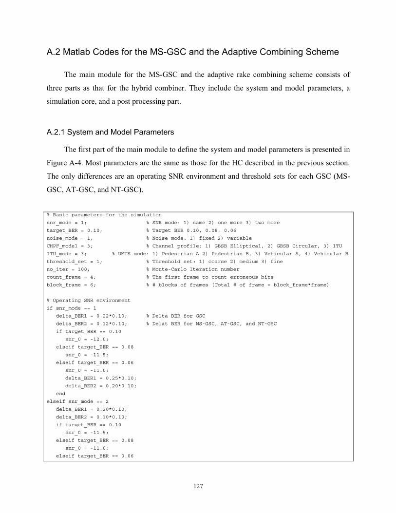
127
A.2 Matlab Codes for the MS-GSC and the Adaptive Combining Scheme
The main module for the MS-GSC and the adaptive rake combining scheme consists of
three parts as that for the hybrid combiner. They include the system and model parameters, a
simulation core, and a post processing part.
A.2.1 System and Model Parameters
The first part of the main module to define the system and model parameters is presented in
Figure A-4. Most parameters are the same as those for the HC described in the previous section.
The only differences are an operating SNR environment and threshold sets for each GSC (MS-
GSC, AT-GSC, and NT-GSC).
% Basic parameters for the simulation
snr_mode = 1; % SNR mode: 1) same 2) one more 3) two more
target_BER = 0.10; % Target BER 0.10, 0.08, 0.06
noise_mode = 1; % Noise mode: 1) fixed 2) variable
CHPF_model = 3; % Channel profile: 1) GBSB Elliptical, 2) GBSB Circular, 3) ITU
ITU_mode = 3; % UMTS mode: 1) Pedestrian A 2) Pedestrian B, 3) Vehicular A, 4) Vehicular B
threshold_set = 1; % Threshold set: 1) coarse 2) medium 3) fine
no_iter = 100; % Monte-Carlo Iteration number
count_frame = 4; % The first frame to count erroneous bits
block_frame = 6; % # blocks of frames (Total # of frame = block_frame*frame)
% Operating SNR environment
if snr_mode == 1
delta_BER1 = 0.22*0.10; % Delta BER for GSC
delta_BER2 = 0.12*0.10; % Delat BER for MS-GSC, AT-GSC, and NT-GSC
if target_BER == 0.10
snr_0 = -12.0;
elseif target_BER == 0.08
snr_0 = -11.5;
elseif target_BER == 0.06
snr_0 = -11.0;
delta_BER1 = 0.25*0.10;
delta_BER2 = 0.20*0.10;
end
elseif snr_mode == 2
delta_BER1 = 0.20*0.10;
delta_BER2 = 0.10*0.10;
if target_BER == 0.10
snr_0 = -11.5;
elseif target_BER == 0.08
snr_0 = -11.0;
elseif target_BER == 0.06

128
snr_0 = -10.5;
delta_BER1 = 0.25*0.10;
delta_BER2 = 0.20*0.10
end
elseif snr_mode == 3
if target_BER == 0.10
snr_0 = -11.0;
end
end
if noise_mode == 1
ebno_power = [snr_0];
else
ebno_power = [snr_0-0.5 snr_0 snr_0+0.5];
end
ebno_index = size(ebno_power,2);
no_pilot_sym_avg = 1;
% Channel parameters
if ITU_mode == 1 | ITU_mode == 2
vhr = 3; % velocity of the users (km/h)
elseif ITU_mode == 3 | ITU_mode == 4
vhr = 50;
end
if ITU_mode == 1
L = 4; % # multipaths in the channel
M = 2; % # RAKE fingers (M<=L)
else
L = 6;
if ITU_mode == 2
M = 5;
elseif ITU_mode == 3 | ITU_mode == 4
M = 4;
end
end
OLoop = 5; ILoop = 15;
c_index_init = ceil(M/2);
% Define a threshold set for each GSC
if CHPF_model == 1
msgsc_power = [1.0 2.0 3.0 4.0 5.0 6.0 7.0];
atgsc_power = [5.0 3.0 1.5 1.0 0.6 0.3 0.1];
ntgsc_power = [0.8 0.5 0.3 0.2 0.1 0.05 0.01];
elseif CHPF_model == 2
msgsc_power = [1.0 2.0 3.0 4.0 5.0 6.0 7.0];
atgsc_power = [5.0 3.0 1.5 1.0 0.6 0.3 0.1];
ntgsc_power = [0.8 0.5 0.3 0.2 0.1 0.05 0.01];
elseif CHPF_model == 3
if threshold_set == 1
if ITU_mode == 2
% Threshold set for Pedestrian B with 5 fingers
% Finger saving 4 3.5 3 2.5 2.0 1.5 1.0 0.5 0
msgsc_power = [0.01 1.95 2.68 3.3 4.0 4.8 5.8 7.2 30.0];
atgsc_power = [30.0 1.68 1.1 0.81 0.61 0.44 0.3 0.17 0.000001];

129
ntgsc_power = [0.99999 0.74 0.54 0.38 0.275 0.19 0.125 0.065 0.000001];
else
% Threshold set for Vehicular A with 4 fingers
% Finger saving 3 2.5 2.0 1.5 1.0 0.5 0
msgsc_power = [0.01 1.55 2.3 3.15 4.2 5.8 30.0];
atgsc_power = [30.0 1.1 0.62 0.38 0.22 0.1 0.000001];
ntgsc_power = [0.99999 0.54 0.3 0.175 0.1 0.042 0.000001];
end
elseif threshold_set == 2
if ITU_mode == 2
% Threshold set for Pedestrian B with 5 fingers
%msgsc_power = [0.1 1.67 2.23 2.75 3.2 3.8 4.5 5.3 6.5 30.0];
%atgsc_power = [30.0 2.25 1.45 1.1 0.87 0.67 0.5 0.35 0.20 0.001];
%ntgsc_power = [0.99 0.84 0.67 0.53 0.42 0.31 0.22 0.15 0.09 0.001];
% Finger saving 4 3.7 3.3 3 2.7 2.3 2.0 1.7 1.3 1.0 0.7 0.3 0
msgsc_power = [0.01 1.7 2.35 2.68 3.05 3.45 4.05 4.5 5.5 5.8 6.5 8.0 30.0];
atgsc_power = [30.0 2.45 1.5 1.07 0.925 0.75 0.61 0.53 0.4 0.31 0.25 0.1 0.0001];
ntgsc_power = [0.999 0.83 0.69 0.54 0.45 0.35 0.28 0.22 0.18 0.12 0.09 0.03 0.0001];
else
% Threshold set for Vehicular A with 4 fingers
% Finger saving 3 2.7 2.3 2.0 1.7 1.3 1.0 0.7 0.3 0
msgsc_power = [0.01 1.2 1.75 2.3 2.83 3.47 4.2 5.4 7.5 30.0];
atgsc_power = [30.0 1.7 0.95 0.65 0.48 0.35 0.22 0.14 0.07 0.0001];
ntgsc_power = [0.999 0.68 0.47 0.3 0.22 0.15 0.1 0.06 0.03 0.0001];
end
end
end
msgsc_index = size (msgsc_power, 2);
ms_index_init = ceil(msgsc_index/2);
atgsc_index = size (atgsc_power, 2);
at_index_init = ceil(atgsc_index/2);
ntgsc_index = size (ntgsc_power, 2);
nt_index_init = ceil(ntgsc_index/2);
% Downlink WCDMA signal parameters
K = 8; % # users
des_usr_indx = floor(K/2)+1; % Desired user index
sf_no = 13; % slot format number (0-16) for user's DPCH
s_format = slot_format(sf_no); % returns slot format: s_format(1)=sf, s_format(2)= Ndata1,
s_format(3)= Ndata3, s_format(4)= Ntpc, s_format(5)= Ntfci, s_format(6)= Npilot
sf_index = s_format(1); % spreading factor index
sf_user = sf_index.*ones(K,1); % spreading factor for the users DP(D/C)CH (32 for I and Q)
sf_common = 256; % spreading factor for CCPCH
pri_pilot = 1+j; % P-CPICH (Primary Common Pilot Channel) signal
ovsf_code_numb = floor(linspace(3,sf_index,K))';
block_frame = 4; % # blocks of frames (Total # of frame = block_frame*frame)
frame = 1; % # frames in a block of frames
slot_frame = 15; % # slots per frame
pilot_slot = s_format(6); % # pilot symbols per slot
chip_frame = 38400; % # chips per frame
samp_chip = 4; % # samples per chip
% Downlink OVSF and long scrambling codes
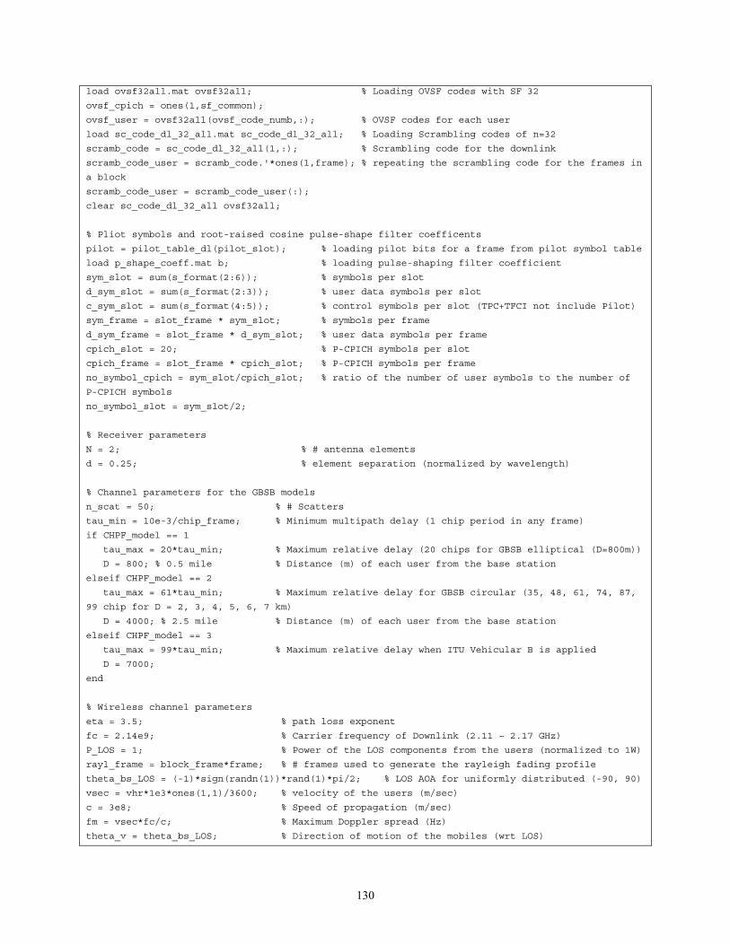
130
load ovsf32all.mat ovsf32all; % Loading OVSF codes with SF 32
ovsf_cpich = ones(1,sf_common);
ovsf_user = ovsf32all(ovsf_code_numb,:); % OVSF codes for each user
load sc_code_dl_32_all.mat sc_code_dl_32_all; % Loading Scrambling codes of n=32
scramb_code = sc_code_dl_32_all(1,:); % Scrambling code for the downlink
scramb_code_user = scramb_code.'*ones(1,frame); % repeating the scrambling code for the frames in
a block
scramb_code_user = scramb_code_user(:);
clear sc_code_dl_32_all ovsf32all;
% Pliot symbols and root-raised cosine pulse-shape filter coefficents
pilot = pilot_table_dl(pilot_slot); % loading pilot bits for a frame from pilot symbol table
load p_shape_coeff.mat b; % loading pulse-shaping filter coefficient
sym_slot = sum(s_format(2:6)); % symbols per slot
d_sym_slot = sum(s_format(2:3)); % user data symbols per slot
c_sym_slot = sum(s_format(4:5)); % control symbols per slot (TPC+TFCI not include Pilot)
sym_frame = slot_frame * sym_slot; % symbols per frame
d_sym_frame = slot_frame * d_sym_slot; % user data symbols per frame
cpich_slot = 20; % P-CPICH symbols per slot
cpich_frame = slot_frame * cpich_slot; % P-CPICH symbols per frame
no_symbol_cpich = sym_slot/cpich_slot; % ratio of the number of user symbols to the number of
P-CPICH symbols
no_symbol_slot = sym_slot/2;
% Receiver parameters
N = 2; % # antenna elements
d = 0.25; % element separation (normalized by wavelength)
% Channel parameters for the GBSB models
n_scat = 50; % # Scatters
tau_min = 10e-3/chip_frame; % Minimum multipath delay (1 chip period in any frame)
if CHPF_model == 1
tau_max = 20*tau_min; % Maximum relative delay (20 chips for GBSB elliptical (D=800m))
D = 800; % 0.5 mile % Distance (m) of each user from the base station
elseif CHPF_model == 2
tau_max = 61*tau_min; % Maximum relative delay for GBSB circular (35, 48, 61, 74, 87,
99 chip for D = 2, 3, 4, 5, 6, 7 km)
D = 4000; % 2.5 mile % Distance (m) of each user from the base station
elseif CHPF_model == 3
tau_max = 99*tau_min; % Maximum relative delay when ITU Vehicular B is applied
D = 7000;
end
% Wireless channel parameters
eta = 3.5; % path loss exponent
fc = 2.14e9; % Carrier frequency of Downlink (2.11 ~ 2.17 GHz)
P_LOS = 1; % Power of the LOS components from the users (normalized to 1W)
rayl_frame = block_frame*frame; % # frames used to generate the rayleigh fading profile
theta_bs_LOS = (-1)*sign(randn(1))*rand(1)*pi/2; % LOS AOA for uniformly distributed (-90, 90)
vsec = vhr*1e3*ones(1,1)/3600; % velocity of the users (m/sec)
c = 3e8; % Speed of propagation (m/sec)
fm = vsec*fc/c; % Maximum Doppler spread (Hz)
theta_v = theta_bs_LOS; % Direction of motion of the mobiles (wrt LOS)

131
% Received signal at Mobile Station
fs = chip_frame*samp_chip*100; % Sampling rate of the transmitted baseband signal (10ms frame)
max_delay = floor(tau_max*fs); % maximum multipath delay in samples
signal_block = frame*chip_frame*samp_chip; % length of the signal observation window in samples
% Power budget for the common pilot (20%)
K_pilot = floor(K/4);
P_ratio = sqrt(K_pilot)/2;
Other_Power = K_pilot + K - 1;
Figure A-4 System and Model Parameters for the GSCs
A.2.2 Simulation Core
The second part of the main module is a simulation core, which is presented in Figure A-5.
This simulation core consists of several loops. The most outer loop specifies the number of
iterations. The second outer loop is for different SNRs. The third outer loop repeats for a number
of frames for each simulation run. There are several inner loops in this third outer loop. The first
and the second inner loops are to generate the transmitted user signal and to generate multipath
signals for this user signal, respectively. The third inner loop is to despread each multipath signal
using a rake finger, while the last inner loop is to find a moving average of signal power for each
pilot symbol.
for iter = 1:no_iter %% loop 1
c_index1 = c_index_init; c_index2 = c_index_init;
ms_index1 = ms_index_init; ms_index2 = ms_index_init;
at_index1 = at_index_init; at_index2 = at_index_init;
nt_index1 = nt_index_init; nt_index2 = nt_index_init;
theta_bs_LOS = (-1)*sign(randn(1))*rand(1)*pi/2;
if CHPF_model == 1
[tau,theta_bs,P,alpha] = …
vec_ch_ellip_dl_1(n_scat,L,D,tau_max,tau_min,P_LOS,theta_bs_LOS,eta);
elseif CHPF_model == 2
[tau,theta_bs,P,alpha] = …
vec_ch_circ_dl_1(n_scat,L,D,tau_max,tau_min,P_LOS,theta_bs_LOS,eta);
elseif CHPF_model == 3
[tau,theta_bs,P,alpha] = …
vec_ch_umts_dl_1(n_scat,L,D,tau_max,tau_min,P_LOS,theta_bs_LOS,eta,ITU_mode);
end
tau_samp = round(tau*fs); % multipath delays in chip samples
fd = abs(fm*cos(theta_bs-theta_v)); % doppler spread for each multipath
I = find(fd < 1); % If doppler spread < 1 map it to 1
fd(I) = 1;
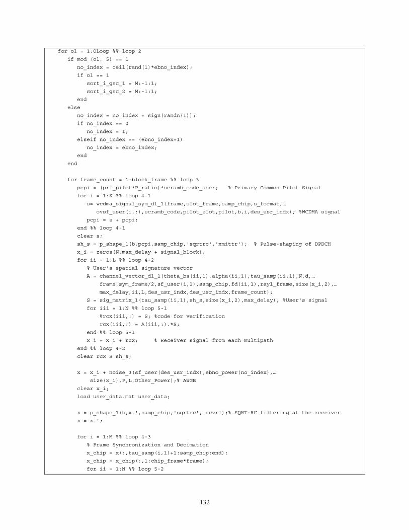
132
for ol = 1:OLoop %% loop 2
if mod (ol, 5) == 1
no_index = ceil(rand(1)*ebno_index);
if ol == 1
sort_i_gsc_1 = M:-1:1;
sort_i_gsc_2 = M:-1:1;
end
else
no_index = no_index + sign(randn(1));
if no_index == 0
no_index = 1;
elseif no_index == (ebno_index+1)
no_index = ebno_index;
end
end
for frame_count = 1:block_frame %% loop 3
pcpi = (pri_pilot*P_ratio)*scramb_code_user; % Primary Common Pilot Signal
for i = 1:K %% loop 4-1
s= wcdma_signal_sym_dl_1(frame,slot_frame,samp_chip,s_format,…
ovsf_user(i,:),scramb_code,pilot_slot,pilot,b,i,des_usr_indx); %WCDMA signal
pcpi = s + pcpi;
end %% loop 4-1
clear s;
sh_s = p_shape_1(b,pcpi,samp_chip,'sqrtrc','xmittr'); % Pulse-shaping of DPDCH
x_i = zeros(N,max_delay + signal_block);
for ii = 1:L %% loop 4-2
% User's spatial signature vector
A = channel_vector_dl_1(theta_bs(ii,1),alpha(ii,1),tau_samp(ii,1),N,d,…
frame,sym_frame/2,sf_user(i,1),samp_chip,fd(ii,1),rayl_frame,size(x_i,2),…
max_delay,ii,L,des_usr_indx,des_usr_indx,frame_count);
S = sig_matrix_1(tau_samp(ii,1),sh_s,size(x_i,2),max_delay); %User's signal
for iii = 1:N %% loop 5-1
%rcx(iii,:) = S; %code for verification
rcx(iii,:) = A(iii,:).*S;
end %% loop 5-1
x_i = x_i + rcx; % Receiver signal from each multipath
end %% loop 4-2
clear rcx S sh_s;
x = x_i + noise_3(sf_user(des_usr_indx),ebno_power(no_index),…
size(x_i),P,L,Other_Power);% AWGB
clear x_i;
load user_data.mat user_data;
x = p_shape_1(b,x.',samp_chip,'sqrtrc','rcvr');% SQRT-RC filtering at the receiver
x = x.';
for i = 1:M %% loop 4-3
% Frame Synchronization and Decimation
x_chip = x(:,tau_samp(i,1)+1:samp_chip:end);
x_chip = x_chip(:,1:chip_frame*frame);
for ii = 1:N %% loop 5-2
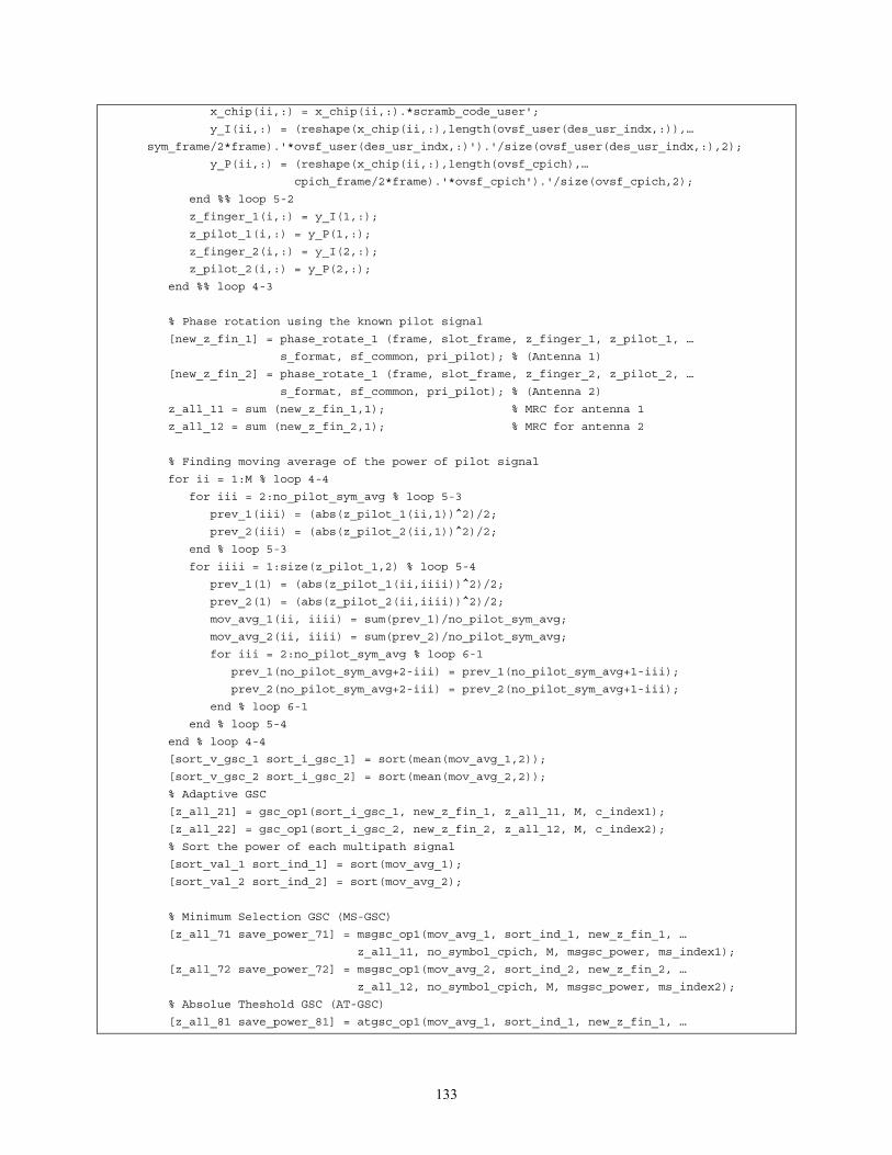
133
x_chip(ii,:) = x_chip(ii,:).*scramb_code_user';
y_I(ii,:) = (reshape(x_chip(ii,:),length(ovsf_user(des_usr_indx,:)),…
sym_frame/2*frame).'*ovsf_user(des_usr_indx,:)').'/size(ovsf_user(des_usr_indx,:),2);
y_P(ii,:) = (reshape(x_chip(ii,:),length(ovsf_cpich),…
cpich_frame/2*frame).'*ovsf_cpich').'/size(ovsf_cpich,2);
end %% loop 5-2
z_finger_1(i,:) = y_I(1,:);
z_pilot_1(i,:) = y_P(1,:);
z_finger_2(i,:) = y_I(2,:);
z_pilot_2(i,:) = y_P(2,:);
end %% loop 4-3
% Phase rotation using the known pilot signal
[new_z_fin_1] = phase_rotate_1 (frame, slot_frame, z_finger_1, z_pilot_1, …
s_format, sf_common, pri_pilot); % (Antenna 1)
[new_z_fin_2] = phase_rotate_1 (frame, slot_frame, z_finger_2, z_pilot_2, …
s_format, sf_common, pri_pilot); % (Antenna 2)
z_all_11 = sum (new_z_fin_1,1); % MRC for antenna 1
z_all_12 = sum (new_z_fin_2,1); % MRC for antenna 2
% Finding moving average of the power of pilot signal
for ii = 1:M % loop 4-4
for iii = 2:no_pilot_sym_avg % loop 5-3
prev_1(iii) = (abs(z_pilot_1(ii,1))^2)/2;
prev_2(iii) = (abs(z_pilot_2(ii,1))^2)/2;
end % loop 5-3
for iiii = 1:size(z_pilot_1,2) % loop 5-4
prev_1(1) = (abs(z_pilot_1(ii,iiii))^2)/2;
prev_2(1) = (abs(z_pilot_2(ii,iiii))^2)/2;
mov_avg_1(ii, iiii) = sum(prev_1)/no_pilot_sym_avg;
mov_avg_2(ii, iiii) = sum(prev_2)/no_pilot_sym_avg;
for iii = 2:no_pilot_sym_avg % loop 6-1
prev_1(no_pilot_sym_avg+2-iii) = prev_1(no_pilot_sym_avg+1-iii);
prev_2(no_pilot_sym_avg+2-iii) = prev_2(no_pilot_sym_avg+1-iii);
end % loop 6-1
end % loop 5-4
end % loop 4-4
[sort_v_gsc_1 sort_i_gsc_1] = sort(mean(mov_avg_1,2));
[sort_v_gsc_2 sort_i_gsc_2] = sort(mean(mov_avg_2,2));
% Adaptive GSC
[z_all_21] = gsc_op1(sort_i_gsc_1, new_z_fin_1, z_all_11, M, c_index1);
[z_all_22] = gsc_op1(sort_i_gsc_2, new_z_fin_2, z_all_12, M, c_index2);
% Sort the power of each multipath signal
[sort_val_1 sort_ind_1] = sort(mov_avg_1);
[sort_val_2 sort_ind_2] = sort(mov_avg_2);
% Minimum Selection GSC (MS-GSC)
[z_all_71 save_power_71] = msgsc_op1(mov_avg_1, sort_ind_1, new_z_fin_1, …
z_all_11, no_symbol_cpich, M, msgsc_power, ms_index1);
[z_all_72 save_power_72] = msgsc_op1(mov_avg_2, sort_ind_2, new_z_fin_2, …
z_all_12, no_symbol_cpich, M, msgsc_power, ms_index2);
% Absolue Theshold GSC (AT-GSC)
[z_all_81 save_power_81] = atgsc_op1(mov_avg_1, sort_ind_1, new_z_fin_1, …

134
z_all_11, no_symbol_cpich, M, atgsc_power, at_index1);
[z_all_82 save_power_82] = atgsc_op1(mov_avg_2, sort_ind_2, new_z_fin_2, …
z_all_12, no_symbol_cpich, M, atgsc_power, at_index2);
% Normalzied Theshold GSC (NT-GSC)
[z_all_91 save_power_91] = ntgsc_op1(mov_avg_1, sort_ind_1, new_z_fin_1, …
z_all_11, no_symbol_cpich, M, ntgsc_power, nt_index1);
[z_all_92 save_power_92] = ntgsc_op1(mov_avg_2, sort_ind_2, new_z_fin_2, …
z_all_12, no_symbol_cpich, M, ntgsc_power, nt_index2);
% Hard decision for data detection of I/Q channel
z_I_11 = sign(real(z_all_11)); z_Q_11 = sign(imag(z_all_11));
z_I_12 = sign(real(z_all_12)); z_Q_12 = sign(imag(z_all_12));
z_I_21 = sign(real(z_all_21)); z_Q_21 = sign(imag(z_all_21));
z_I_22 = sign(real(z_all_22)); z_Q_22 = sign(imag(z_all_22));
z_I_71 = sign(real(z_all_71)); z_Q_71 = sign(imag(z_all_71));
z_I_72 = sign(real(z_all_72)); z_Q_72 = sign(imag(z_all_72));
z_I_81 = sign(real(z_all_81)); z_Q_81 = sign(imag(z_all_81));
z_I_82 = sign(real(z_all_82)); z_Q_82 = sign(imag(z_all_82));
z_I_91 = sign(real(z_all_91)); z_Q_91 = sign(imag(z_all_91));
z_I_92 = sign(real(z_all_92)); z_Q_92 = sign(imag(z_all_92));
z_I_11 = z_I_11(:); z_Q_11 = z_Q_11(:);
z_I_12 = z_I_12(:); z_Q_12 = z_Q_12(:);
z_I_21 = z_I_21(:); z_Q_21 = z_Q_21(:);
z_I_22 = z_I_22(:); z_Q_22 = z_Q_22(:);
z_I_71 = z_I_71(:); z_Q_71 = z_Q_71(:);
z_I_72 = z_I_72(:); z_Q_72 = z_Q_72(:);
z_I_81 = z_I_81(:); z_Q_81 = z_Q_81(:);
z_I_82 = z_I_82(:); z_Q_82 = z_Q_82(:);
z_I_91 = z_I_91(:); z_Q_91 = z_Q_91(:);
z_I_92 = z_I_92(:); z_Q_92 = z_Q_92(:);
% Data extraction
data_out_11=extract_data (frame,slot_frame,z_I_11,z_Q_11,s_format); % MRC-Ant 1
data_out_12=extract_data (frame,slot_frame,z_I_12,z_Q_12,s_format); % MRC-Ant 2
data_out_21=extract_data (frame,slot_frame,z_I_21,z_Q_21,s_format); % GSC-Ant 1
data_out_22=extract_data (frame,slot_frame,z_I_22,z_Q_22,s_format); % GSC-Ant 2
data_out_71=extract_data (frame,slot_frame,z_I_71,z_Q_71,s_format); % MS_GSC-Ant 1
data_out_72=extract_data (frame,slot_frame,z_I_72,z_Q_72,s_format); % MS_GSC-Ant 2
data_out_81=extract_data (frame,slot_frame,z_I_81,z_Q_81,s_format); % AT-GSC-Ant 1
data_out_82=extract_data (frame,slot_frame,z_I_82,z_Q_82,s_format); % AT-GSC-Ant 2
data_out_91=extract_data (frame,slot_frame,z_I_91,z_Q_91,s_format); % NT-GSC-Ant 1
data_out_92=extract_data (frame,slot_frame,z_I_92,z_Q_92,s_format); % NT-GSC-Ant 2
% Number of error symbols
Nerror_11(frame_count,1) = length(find(data_out_11 ~= user_data));
Nerror_12(frame_count,1) = length(find(data_out_12 ~= user_data));
Nerror_21(frame_count,1) = length(find(data_out_21 ~= user_data));
Nerror_22(frame_count,1) = length(find(data_out_22 ~= user_data));
Nerror_71(frame_count,1) = length(find(data_out_71 ~= user_data));
Nerror_72(frame_count,1) = length(find(data_out_72 ~= user_data));
Nerror_81(frame_count,1) = length(find(data_out_81 ~= user_data));
Nerror_82(frame_count,1) = length(find(data_out_82 ~= user_data));
Nerror_91(frame_count,1) = length(find(data_out_91 ~= user_data));
Nerror_92(frame_count,1) = length(find(data_out_92 ~= user_data));
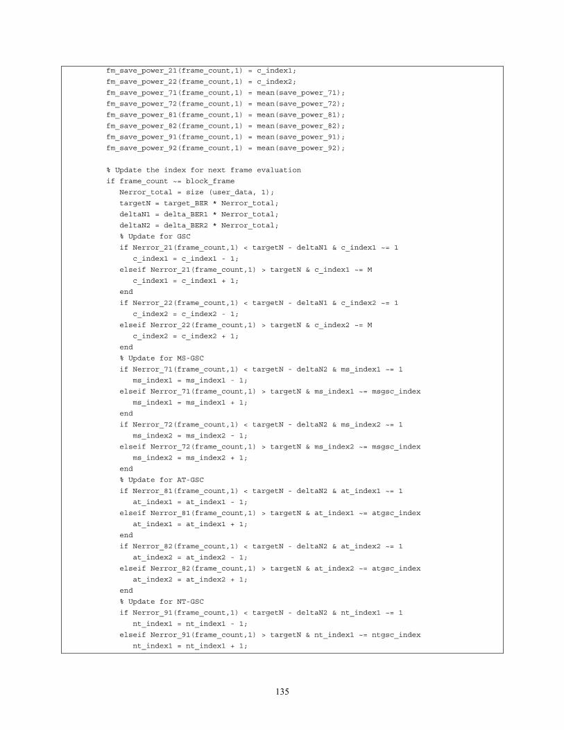
135
fm_save_power_21(frame_count,1) = c_index1;
fm_save_power_22(frame_count,1) = c_index2;
fm_save_power_71(frame_count,1) = mean(save_power_71);
fm_save_power_72(frame_count,1) = mean(save_power_72);
fm_save_power_81(frame_count,1) = mean(save_power_81);
fm_save_power_82(frame_count,1) = mean(save_power_82);
fm_save_power_91(frame_count,1) = mean(save_power_91);
fm_save_power_92(frame_count,1) = mean(save_power_92);
% Update the index for next frame evaluation
if frame_count ~= block_frame
Nerror_total = size (user_data, 1);
targetN = target_BER * Nerror_total;
deltaN1 = delta_BER1 * Nerror_total;
deltaN2 = delta_BER2 * Nerror_total;
% Update for GSC
if Nerror_21(frame_count,1) < targetN - deltaN1 & c_index1 ~= 1
c_index1 = c_index1 - 1;
elseif Nerror_21(frame_count,1) > targetN & c_index1 ~= M
c_index1 = c_index1 + 1;
end
if Nerror_22(frame_count,1) < targetN - deltaN1 & c_index2 ~= 1
c_index2 = c_index2 - 1;
elseif Nerror_22(frame_count,1) > targetN & c_index2 ~= M
c_index2 = c_index2 + 1;
end
% Update for MS-GSC
if Nerror_71(frame_count,1) < targetN - deltaN2 & ms_index1 ~= 1
ms_index1 = ms_index1 - 1;
elseif Nerror_71(frame_count,1) > targetN & ms_index1 ~= msgsc_index
ms_index1 = ms_index1 + 1;
end
if Nerror_72(frame_count,1) < targetN - deltaN2 & ms_index2 ~= 1
ms_index2 = ms_index2 - 1;
elseif Nerror_72(frame_count,1) > targetN & ms_index2 ~= msgsc_index
ms_index2 = ms_index2 + 1;
end
% Update for AT-GSC
if Nerror_81(frame_count,1) < targetN - deltaN2 & at_index1 ~= 1
at_index1 = at_index1 - 1;
elseif Nerror_81(frame_count,1) > targetN & at_index1 ~= atgsc_index
at_index1 = at_index1 + 1;
end
if Nerror_82(frame_count,1) < targetN - deltaN2 & at_index2 ~= 1
at_index2 = at_index2 - 1;
elseif Nerror_82(frame_count,1) > targetN & at_index2 ~= atgsc_index
at_index2 = at_index2 + 1;
end
% Update for NT-GSC
if Nerror_91(frame_count,1) < targetN - deltaN2 & nt_index1 ~= 1
nt_index1 = nt_index1 - 1;
elseif Nerror_91(frame_count,1) > targetN & nt_index1 ~= ntgsc_index
nt_index1 = nt_index1 + 1;

136
end
if Nerror_92(frame_count,1) < targetN - deltaN2 & nt_index2 ~= 1
nt_index2 = nt_index2 - 1;
elseif Nerror_92(frame_count,1) > targetN & nt_index2 ~= ntgsc_index
nt_index2 = nt_index2 + 1;
end
end
end %% loop 3
% Symbol error rate
Ne_I_11(ol,iter) = sum(Nerror_11(count_frame:end),1);
Ne_I_12(ol,iter) = sum(Nerror_12(count_frame:end),1);
Ne_I_21(ol,iter) = sum(Nerror_21(count_frame:end),1);
Ne_I_22(ol,iter) = sum(Nerror_22(count_frame:end),1);
Ne_I_71(ol,iter) = sum(Nerror_71(count_frame:end),1);
Ne_I_72(ol,iter) = sum(Nerror_72(count_frame:end),1);
Ne_I_81(ol,iter) = sum(Nerror_81(count_frame:end),1);
Ne_I_82(ol,iter) = sum(Nerror_82(count_frame:end),1);
Ne_I_91(ol,iter) = sum(Nerror_91(count_frame:end),1);
Ne_I_92(ol,iter) = sum(Nerror_92(count_frame:end),1);
% Finger saving
DF_S_21(ol,iter) = mean(fm_save_power_21(count_frame:end),1);
DF_S_22(ol,iter) = mean(fm_save_power_22(count_frame:end),1);
DF_S_71(ol,iter) = mean(fm_save_power_71(count_frame:end),1);
DF_S_72(ol,iter) = mean(fm_save_power_72(count_frame:end),1);
DF_S_81(ol,iter) = mean(fm_save_power_81(count_frame:end),1);
DF_S_82(ol,iter) = mean(fm_save_power_82(count_frame:end),1);
DF_S_91(ol,iter) = mean(fm_save_power_91(count_frame:end),1);
DF_S_92(ol,iter) = mean(fm_save_power_92(count_frame:end),1);
end %% loop 2
end %% loop 1
Figure A-5 Simulation Core for the GSCs
The simulation core contains almost the same functions as those for the HC. The only
difference is that there are several GSC functions to combine each finger signal depending on the
combining scheme of each GSC method. Functions to evaluate the current BER after each frame
and to dynamically adjust the threshold values for each GSC method are included in this
simulation core.
A.2.3 Post Processing
The last part of the main module is presented in Figure A-6. It consists of three sub-parts.
They are almost the same as those for the HC. The only difference is that the first sub-part also
includes the calculation of finger saving for each GSC method.

137
% BERs and finger savings for each GSC method
total_no_iter = no_iter*OLoop;
no_sym_iter = d_sym_frame*frame*(block_frame-count_frame+1)*total_no_iter;
Ps_av_11 = sum(sum(Ne_I_11,2))/no_sym_iter;
Ps_av_12 = sum(sum(Ne_I_12,2))/no_sym_iter;
Ps_av_21 = sum(sum(Ne_I_21,2))/no_sym_iter;
Ps_av_22 = sum(sum(Ne_I_22,2))/no_sym_iter;
Ps_av_71 = sum(sum(Ne_I_71,2))/no_sym_iter;
Ps_av_72 = sum(sum(Ne_I_72,2))/no_sym_iter;
Ps_av_81 = sum(sum(Ne_I_81,2))/no_sym_iter;
Ps_av_82 = sum(sum(Ne_I_82,2))/no_sym_iter;
Ps_av_91 = sum(sum(Ne_I_91,2))/no_sym_iter;
Ps_av_92 = sum(sum(Ne_I_92,2))/no_sym_iter;
Pp_av_21 = M - sum(sum(DF_S_21,2))/total_no_iter;
Pp_av_22 = M - sum(sum(DF_S_22,2))/total_no_iter;
Pp_av_71 = M - sum(sum(DF_S_71,2))/total_no_iter;
Pp_av_72 = M - sum(sum(DF_S_72,2))/total_no_iter;
Pp_av_81 = M - sum(sum(DF_S_81,2))/total_no_iter;
Pp_av_82 = M - sum(sum(DF_S_82,2))/total_no_iter;
Pp_av_91 = M - sum(sum(DF_S_91,2))/total_no_iter;
Pp_av_92 = M - sum(sum(DF_S_92,2))/total_no_iter;
% Defene a file name to save the simulation results
if noise_mode == 1
sim_mode = 'CLGSC_fn';
else
sim_mode = 'CLGSC_vn';
end
if CHPF_model == 1
file_head = 'ell';
elseif CHPF_model == 2
file_head = 'cir';
elseif CHPF_model == 3
if snr_mode == 1
if ITU_mode == 1
file_head = 'umts_pa';
elseif ITU_mode == 2
file_head = 'umts_pb';
elseif ITU_mode == 3
file_head = 'umts_va';
elseif ITU_mode == 4
file_head = 'umts_vb';
end
elseif snr_mode == 2
if ITU_mode == 1
file_head = 'umts_pa_s1';
elseif ITU_mode == 2
file_head = 'umts_pb_s1';
elseif ITU_mode == 3
file_head = 'umts_va_s1';
elseif ITU_mode == 4
file_head = 'umts_vb_s1';

138
end
elseif snr_mode == 3
if ITU_mode == 1
file_head = 'umts_pa_s2';
elseif ITU_mode == 2
file_head = 'umts_pb_s2';
elseif ITU_mode == 3
file_head = 'umts_va_s2';
elseif ITU_mode == 4
file_head = 'umts_vb_s2';
end
end
end
if target_BER == 0.1
t_ber = 't10';
elseif target_BER == 0.09
t_ber = 't09';
elseif target_BER == 0.08
t_ber = 't08';
elseif target_BER == 0.07
t_ber = 't07';
elseif target_BER == 0.06
t_ber = 't06';
elseif target_BER == 0.05
t_ber = 't05';
elseif target_BER == 0.04
t_ber = 't04';
elseif target_BER == 0.11
t_ber = 't11';
elseif target_BER == 0.12
t_ber = 't12';
end
% Save the simulation results into the file
[outfilename,errormessage] = sprintf('BER_%s_%s_%s_v%d_M%d',sim_mode,file_head,t_ber,vhr,M);
save(outfilename,'M','no_iter','total_no_iter','*_power','Ps_av_*','Pp_av_*','Ne_I_*', 'DF_S_*');
Figure A-6 Post Processing for the GSCs

139
Vita
SUK WON KIM
Suk Won Kim was born in Yongin, Korea on May 4, 1964. He received the Bachelor of
Science and Master of Science degrees in Mathematics from Seoul National University, Seoul,
Korea in 1987 and 1991, respectively. He received another Master of Science degree in
Electrical Engineering from the University of California at Los Angles (UCLA), Los Angeles,
CA in 1999. From 1991 to 1995, he worked at the Semiconductor Division of Samsung
Electronic Co., Ltd., Kiheung, Korea, where he was involved in the development of ASIC CAD
tools and cell libraries. In 1999, he started his Ph.D. program at Virginia Polytechnic Institute
and State University, Blacksburg, VA. He was awarded a scholarship from Samsung Electronic
Co., Ltd. for pursuing his Ph.D. degree. His research interests include ASIC design for wireless
communication systems, low-power VLSI design, and smart antennas for the third generation
wideband CDMA systems.