small sample properties of bayesian estimators of labor income
TRANSCRIPT

Small Sample Properties of Bayesian Estimators
of Labor Income Processes∗
Taisuke Nakata†
Federal Reserve Board
Christopher Tonetti‡
Stanford GSB
March 31, 2014
Abstract
There exists an extensive literature estimating idiosyncratic labor income processes. While a wide
variety of models are estimated, GMM estimators are almost always used. We examine the validity
of using likelihood based estimation in this context by comparing the small sample properties of a
Bayesian estimator to those of GMM. Our baseline studies estimators of a commonly used simple
earnings process. We extend our analysis to more complex environments, allowing for real world
phenomena such as time varying and heterogeneous parameters, missing data, unbalanced panels,
and non-normal errors. The Bayesian estimators are demonstrated to have favorable bias and
efficiency properties.
JEL: C32, C33, D12, D31, D91, E21
Keywords: Labor Income Process, Small Sample Properties, GMM, Bayesian Estimation, Error
Component Models
∗We thank Tim Cogley, Konrad Menzel, John Roberts, Tom Sargent, Matt Smith, and Gianluca Violante for usefulcomments and suggestions. The views expressed in this paper, and all errors and omissions, should be regarded asthose solely of the authors, and are not necessarily those of the Federal Reserve Board of Governors or the FederalReserve System.
†Corresponding author; Division of Research and Statistics, Federal Reserve Board, 20th Street and ConstitutionAvenue N.W. Washington, D.C. 20551; Email: [email protected]; Phone: 202-452-2972.
‡Stanford GSB, 655 Knight Way, Stanford, CA 94305; Email: [email protected].
1

1 Introduction
Measuring individual income risk is essential to answering a wide range of economic questions.
For the vast majority of individuals, labor income is overwhelmingly the largest component of total
income. Accordingly, accurate and precise estimation of labor earnings dynamics is important for
analyzing people’s consumption and savings behavior, designing fiscal policy, and understanding
the sources of and changes in inequality.
Dating back to Lillard and Willis (1978), Lillard and Weiss (1979), MaCurdy (1982), and Abowd
and Card (1989), there is a history of fitting ARMA models to panel data to understand the labor
income risk facing individuals. Error component models in which labor income is the sum of a
transitory and a persistent shock are extremely common.1 While no shortage of models have been
estimated, a striking feature of the literature is that, almost always, the estimation routine is based
on a minimum distance estimator, namely GMM.
Recent trends of increasing model complexity have led economists to depart from the sim-
ple GMM estimators that have dominated the literature. Sometimes these complex models are
estimated by techniques similar to traditional GMM, like the Simulated Method of Moments.2
However, sometimes a very different likelihood based approach, Bayesian estimation, is employed.
An early example using Bayesian estimation is Geweke and Keane (2000), who jointly estimate
earnings process parameters and marital status to analyze the transition probabilities between in-
come quartiles over the life cycle. More recently, Jensen and Shore (2010, 2011) estimate complex
labor income processes with a focus on heterogeneity in idiosyncratic risk and its evolution over
time. Given ongoing advances in computational power and Markov chain Monte Carlo (MCMC)
techniques, we are likely to see a growing use of these estimators.
While there exist decades of research that documents the properties of minimum distance es-
timators of labor income processes, there are no papers, to our knowledge, that systematically
examine the small sample properties of likelihood based estimators on these types of error com-
ponent models in panel settings.3 Although the benefits of Bayesian estimation are well known to
theoretical econometricians, they are not widely understood across fields in the context of estimat-
ing labor income processes. Thus, as the profession adopts widespread use of Bayesian estimators
for increasingly elaborate models, it is useful to document the properties of Bayesian estimators on
simple income processes. This will provide a clear explanation of the Bayesian estimation routine,
a better understanding of the source of estimation results, and a justification for its use in more
complicated settings.
In this paper, we examine the validity of using likelihood based estimation by comparing the
1Often the persistent component is assumed to follow a random walk as in MaCurdy (1982), Abowd and Card(1989), Gottschalk and Moffitt (1994), Meghir and Pistaferri (2004), and Blundell, Pistaferri, and Preston (2008).
2For example, Browning, Ejrnaes, and Alvarez (2010) estimate a model with many dimensions of heterogeneityusing the Simulated Method of Moments.
3For example, a 1996 issue of the Journal of Business & Economic Statistics is dedicated to the small sampleproperties of GMM estimators, featuring notable papers on estimating covariance structures like Altonji and Segal(1996) and Clark (1996).
2

small sample properties of a Bayesian estimator to those of GMM. First, as a stepping stone, we
derive the maximum likelihood estimator by translating the labor income process into linear Gaus-
sian state space (LGSS) form and applying standard filtering procedures. With this machinery
established in an easy-to-understand framework, we provide a concise, but self-contained, deriva-
tion of the Bayesian estimator. We then conduct a Monte Carlo analysis of a Bayesian estimator
and a GMM estimator on a commonly used simple labor income process. Although the asymp-
totic dominance of properly specified likelihood based estimators is textbook, we provide the first
systematic analysis of the small sample properties of likelihood based estimators of labor income
processes. While the difference between estimators is typically modest, the Bayesian estimator is
more efficient: parameter estimates are unbiased with smaller standard errors.
Although the initial findings demonstrate the better small sample properties of the Bayesian
estimator, the exercise was performed on a simple model with ideal dataset conditions. In Section
4, we extend the analysis to more complex specifications that capture real world phenomena. In
Section 4.1, we first look at an environment in which datasets are unbalanced panels and suffer
from missing data. We modify the estimators to accommodate these realistic features of the dataset
and study how the relative performance of the Bayesian estimator is affected. In Section 4.2, we
modify the labor income process to allow for time-variation in the shock variances. Time variation
in the variances of the labor income process has been documented in many papers and is essential in
understanding the changes in labor market risks.4 In Section 4.3, we allow parameter heterogeneity
across individuals. Many papers have found substantial heterogeneity in various aspects of the labor
income process and emphasized its importance for understanding the risks people face. Finally,
in Section 4.4, we extend the labor income process to allow for non-normal shocks. There is
empirical evidence that labor income shocks are non-normal and have fat tails.5 To both learn
about the shape of the error distributions and to address the concern of distribution misspecification,
we let shocks be distributed according to a mixture of normals, which allows for a very flexible
error distribution structure. These extensions establish that the beneficial small sample properties
of Bayesian estimators are maintained in more complicated scenarios—thus demonstrating the
usefulness of this estimator for applied economists.
We proceed in Section 2 to present the different estimators of the simple income process. Sec-
tion 3 discusses their small sample properties and Section 4 discusses extensions to the simple
income process, including time varying variances, missing data, unbalanced panels, heterogeneous
parameters, and distributional assumptions on errors. Section 5 concludes.
4See for example Gottschalk and Moffitt (1994), Heathcote, Perri, and Violante (2010), and Blundell, Pistaferri,and Preston (2008) for GMM based estimations of the sequence of variances.
5See for example Hirano (1998) and Geweke and Keane (2000) for Bayesian estimations of income processes thatallow for non-normal shocks.
3

2 Estimators of the Labor Income Process
It is well known from the labor economics literature (since Abowd and Card (1989)) that labor
income is well described by an error components model, where residual labor earnings are the sum
of a transitory and persistent shock. Often the transitory shock is i.i.d and the persistent shock
follows an AR(1) process. Because the model fits well and is relatively simple, it has become very
commonly used in the Labor and Macro literatures. Thus, we adopt this pervasive simple income
process and present the GMM and Bayesian estimators. These estimators are developed to be used
on panel data sets such as the PSID. Accordingly, our baseline labor income process is given by:
ǫi,t = ρǫi,t−1 +Σ0.5η ηi,t (1)
yi,t = ǫi,t +Σ0.5ν νi,t (2)
where yi,t is the residual from a log income regression for an individual i ∈ {i, ..., N} at time
t ∈ {1, ..., T}.6 ǫi,t is the persistent component of income and is assumed to follow an AR(1) process.
While {yi,t}t=1,Ti=1,N is observed, {ǫi,t}
t=1,Ti=1,N is not. νi,t is the transitory component of income. ηi,t is
the shock to the persistent component of income. νi,t and ηi,t are standard normal and Σν , Ση are
the variances of the transitory and persistent innovations, respectively. We also estimate properties
of the initial state, ǫi,0, which we assume is normally distributed with zero mean and variance
ΣZ0. νi,t, ηi,t, and ǫi,0 are independent of each other for all i and t. Thus the parameter vector
to be estimated is θ := (ρ,Σν ,Ση,ΣZ0). In the next subsections, we outline different techniques to
estimate these parameters.
2.1 GMM
The standard strategy in the literature for estimating labor income processes is to use GMM.
The goal of GMM estimation is to choose parameters that minimize the distance between empirical
and theoretical moments. Identification and estimation rely on moments constructed from cross-
sectional income autocovariances.7
We wish to estimate the system given by equations (1) and (2). There are T (T−1)2 moments,
where T is the total number of time periods. The total number of individuals, N , does not affect
6There are many ways to obtain residual labor income. To remove predictable components that are associatedwith the individual or the aggregate state of the economy, it is common to regress idiosyncratic labor income on avector of observables such as individual demographics and variables that control for aggregates. There are differentmethods to remove aggregate components, such as using time dummy variables or a common correlated effect approach(Pesaran (2006)). While important for the macro implications of the idiosyncratic labor earnings process, our paperis concerned only with estimating the residual labor income process.
7This section develops the already well-understood GMM estimation routine. For other sources see Blundell,Pistaferri, and Preston (2008), Heathcote, Perri, and Violante (2010), or Guvenen (2009). We present the generalcase in which ρ is estimated.
4

the number of moments because the expectations are taken cross-sectionally over individuals.
M(θ) = vec
E[yi,1 · yi,1] ... ... ...
E[yi,2 · yi,1] E[yi,2 · yi,2] ... ...
E[yi,3 · yi,1] E[yi,3 · yi,2] ... ...
...
E[yi,T · yi,1] E[yi,T · yi,2] ... E[yi,T · yi,T ]
where the upper right triangle of the matrix is redundant by symmetry. Particular entries in the
moment matrix M(θ) map into particular functions of the parameters θ = (ρ,Σν ,Ση,ΣZ0). Define
the cross-sectional moment mt,j(θ) between agents at time t and t+ j:
mt,j(θ) = E[yi,t · yi,t+j ]
= E[(ǫi,t +Σ0.5ν νi,t)(ǫi,t+j +Σ0.5
ν νi,t+j)]
=
{
E[ǫ2i,t] + Σν if j = 0
ρjE[ǫ2i,t] if j > 0
where
E[ǫ2i,t] = ρ2tΣZ0 +
t∑
k=1
ρ2(t−k)Ση
Simple algebraic manipulation of the above equations reveal (over) identification of the param-
eters.8
Define the estimator as
θGMM = minθ
(M(θ)− M)′W (M(θ)− M)
where M stacks the sample covariance from the data.
To implement the estimator, we need to choose the weighting matrix, W . Altonji and Segal
(1996) show that the Optimal Minimum Distance (OMD) estimator, where W is the optimal
weighting matrix, introduces significant small sample bias. They study the small sample properties
of the GMM estimator with several alternative weighting matrices and recommend using the Equally
8The moments are only slightly modified when variances are time varying as in Section 4.2:
E[yi,t · yi,t+j ] =
{
E[ǫ2i,t] + Σν,t if j = 0ρjE[ǫ2i,t] if j > 0
E[ǫ2i,t] = ρ2tΣZ0 +
t∑
k=1
ρ2(t−k)Ση,k
5

Weighted Minimum Distance (EWMD) estimator, where W is the identity matrix. In light of their
result, many papers in the literature use the EWMD estimator.9 Thus, we use the GMM estimator
with identity weighting matrix throughout the paper. Extensions to different weighting matrices
are straightforward.10
With all objects of the optimization problem defined, the estimates can be calculated computa-
tionally using an optimizer to choose parameters θ that minimize the distance between model and
sample moments.
2.2 Likelihood Based Estimation
The maximum likelihood estimator is presented before deriving the Bayesian estimator. This
establishes the linear Gaussian state space structure, which is used in both estimators. For the
simple income process, it is feasible to compute the maximum likelihood estimator. However, the
MLE estimator fails to scale with model complexity, as for more complicated specifications the
likelihood is difficult or impossible to write in closed form. Bayesian estimation becomes useful in
exactly these cases.
2.2.1 MLE
As its name suggests, the maximum likelihood estimate is defined as the parameter values that
maximize the likelihood function.
θMLE = maxθ
L({yi,t}t=1,Ti=1,N |θ)
For the simple labor income process, we can analytically compute the likelihood for any given
θ, and thus it is feasible to solve this maximization problem. Analytical derivation of the likelihood
function is straightforward once we notice that the labor income process forms a linear Gaussian
state space (LGSS) system. We can draw from the time series econometrics literature to construct
the likelihood using the Kalman filter.
Define the canonical form of a LGSS as
St = AtSt−1 +Btvt (3)
Yt = Ctzt +DtSt + wt (4)
where
9An alternative used by Blundell, Pistaferri, and Preston (2008) is the Diagonally Weighted Minimum Distance(DWMD) estimator, where W is the optimal weighting matrix with off-diagonal elements set to zero.
10We examined the performance of the OMD and DWMD estimators in unreported exercises and found that theEWMD estimator tends to outperform the OMD and DWMD estimators across various data generating processes.The OMD and DWMD estimators are sometimes slightly more efficient for the persistence parameter than the EWMDestimator, but such improved efficiency in the estimate of the persistence parameter always comes with substantiallydeteriorated efficiency in the estimates of other parameters.
6

vt ∼ N(0, Qt)
wt ∼ N(0, Rt)
S0 ∼ N(S0|0, P0|0)
Equation (3) is the state equation (or transition equation) and equation (4) is the observation
equation (or measurement equation). St is a vector of latent state variables, and Yt is the vector of
observables. vt is a vector of innovations to latent state variables, and wt is a vector of measurement
error. zt is a vector of observed exogenous variables. To map this model into our labor income
process of an individual Yt is residual log income and St is the persistent component of income.11
For notational convenience, let θt be a vector containing all parameters of the model (At, Bt, Ct,
Dt, Qt, Rt, S0|0, P0|0). In many applications, parameters are time-invariant (θt = θ for all t), but
this is not a necessary requirement. All processes discussed in this paper will hold At, Bt, Ct, Dt
constant over time; later, when we discuss the time varying volatility case, Qt and Rt will vary.
Thus, our simple labor income process can be mapped into canonical form as
At = ρ, Bt = 1, Ct = 0,
Dt = 1, Qt = Ση, Rt = Σν,
zt = 0, S0|0 = 0, P0|0 = ΣZ0
for all t, with parameter vector θ = (ρ,Σν ,Ση,ΣZ0) as before.
We can now use the Kalman filter to derive the log likelihood of a LGSS, which is provided
in Appendix A.1.12 As idiosyncratic shocks are defined to be uncorrelated across individuals, one
can obtain the log likelihood of the income data for all individuals by summing the log likelihood
of each individual (i.e., logL({yi,t}t=1,Ti=1,N |θ) =
∑Ni=1 logL({yi,t}
t=1,T |θ)). One obvious advantage
of this methodology is the relative ease of estimating more complicated income processes, such as
ARMA(p,q) processes, since they allow a LGSS representation. Given that the likelihood is defined
in terms of canonical LGSS matrices, to estimate a different parameterization of the labor income
process, all that remains is to map the process into state space form. With the analytical likelihood
derived in Appendix A.1, we can now use an optimizer to numerically maximize the log likelihood
to produce the MLE estimates.
11For clarity of exposition, we set zt to be zero and assume Yt is residual income. However, zt could include all ofthe traditional first stage conditioning variables like education, age, race, etc., to remove the predictable componentsof Yt. This would allow estimation to be run in one step, instead of running a first-stage regression to recoveridiosyncratic residual income. The general case is presented in the Appendix.
12For a detailed analysis, see chapter 13.4 in Hamilton (1994).
7

2.2.2 Bayesian Estimation: Gibbs Sampling
In computing the maximum likelihood estimator, two conditions are crucial. One is that we
can compute the likelihood function analytically and the other is that the likelihood function is
well behaved.13 For the simple labor income process, these two conditions are satisfied and the
MLE estimates can be easily computed. However, they are not satisfied for more complex labor
income processes. Bayesian methods are useful in those cases either because they don’t require
an analytical likelihood function or because the prior distribution smooths local maxima. For
transparency of exposition, in this section we provide an overview of the Bayesian estimator for the
standard income process, without the complications that it is well equipped to handle.
The goal of the Bayesian estimation is to characterize the posterior distribution of parameters,
which is defined as the distribution of parameters conditional on data, p(
θ|{yi,t}t=1,Ti=1,N
)
. The
posterior distribution is related to two objects, the prior distribution and the likelihood function,
by Bayes Theorem:
p(
θ|{yi,t}t=1,Ti=1,N
)
∝ L({yi,t}t=1,Ti=1,N |θ)p(θ)
where p(θ) is the prior distribution of parameters, which the researcher specifies. When the
prior is uniform, the posterior is the same as the likelihood (as a function of parameters). The
tighter the prior, the less the posterior reflects information from the data. Comparing the posterior
to the prior provides a sense of how much the data informed the parameter estimates.14
To characterize the posterior distribution, the Bayesian estimator draws a large sample from
p(
θ|{yi,t}t=1,Ti=1,N
)
, which can be used to compute statistics about the parameters of interest. Once
we characterize the posterior distribution, we can compute a point estimate according to some
loss function. Following other applied work in the Bayesian literature, we use the median of the
posterior distribution as the point estimate.15
To obtain this sample from the posterior, we use the Gibbs sampling algorithm. The Gibbs
sampling algorithm sequentially draws from the distribution of each parameter and latent variable
conditional on the previous draws for all other parameters. Since each draw is conditional on the
previous draws, the samples are not independent. However, the stationary distribution of the draws
thus generated can be shown to equal the joint posterior distribution of interest.16 This algorithm
is useful whenever the joint density of the parameters and data is unknown, but the conditional
distributions of each parameter is known. See Appendix A.2 for details about the Gibbs sampling
procedure.
To sequentially draw from the conditional distributions of interest, there are three techniques
13If there exist multiple local maxima, the optimization routine may struggle to find the global maximum, i.e.,the MLE estimates. This is especially true if the likelihood function is high dimensional.
14See Geweke (2005) or Gelman, Carlin, Stern, and Rubin (2009) for a Bayesian statistics reference.15There is no a priori “correct” statistic to use as the point estimate. For example, one could use the mode, mean,
or median of the posterior distribution. While the mode corresponds closely to the principle of maximum likelihood,the median is more robust computationally when sample sizes are limited.
16See Robert and Casella (2004) for a comprehensive treatment of MCMC theory and practice.
8

employed. The first is estimating the variance of a normal distribution with known mean. The
second is estimating a linear regression model. The third is sampling the latent states of a LGSS
model. To estimate Σν , realize yi,t − ǫi,t = Σ0.5ν νi,t. Thus, conditioning on the epsilon sequence,
we have a sample distributed N(0,Σν). Given a conjugate prior, the posterior can be calculated
analytically, allowing this iteration’s Σν to be set equal to a draw from the conditional posterior. To
estimate ρ, realize from equation 1 that ρ is the coefficient in a linear regression model with known
independent and dependent regressors with error distributed N(0,Ση). Again, the conditional
posterior can be calculated analytically, allowing this iteration’s ρ to be set equal to a draw from
the posterior.
The most complicated Gibbs block of this estimation is drawing the sequence of unobserved
states in a LGSS. Given linearity and normality, the Kalman smoother provides the distribution of
each state at each time conditional on all available data. However, because there is persistence in
the states, knowing the particular draw of ǫi,t alters the conditional density of ǫi,t−1.17 Carter and
Kohn (1994) develop an algorithm that recursively updates, backwards through time, the Kalman
smoothed conditional densities of each state at time t given the draw of the state at time t+ 1.18
With these three tools, we are able to sequentially draw from the conditional distributions of the
parameters and latent variables of interest.
3 Small Sample Properties
Now that the different estimators have been presented, we proceed to analyze the small sample
properties of the estimators using Monte Carlo analysis. Our Monte Carlo simulation exercise
is designed as follows. Simulate 100 panel datasets using the baseline labor income processes
given by equations 1 and 2.19 In the benchmark simulation, each data set contains 500 people
and 10 time periods (i.e., N=500 and T=10). However, to mimic the features of available panel
datasets while also providing a more general depiction of the estimators’ performance, we consider
alternative values of N ∈ {100, 2000} and T ∈ {5, 20}. Motivated by Blundell, Pistaferri, and
Preston (2008), as a benchmark calibration we let the true parameter values be (ρ,Ση,Σν ,ΣZ0) =
(1.00, 0.02, 0.05, 0.15).20 For each of the 100 datasets generated, we compute the point estimates of
the model parameters based on the Bayesian method and the GMM. When required by optimization
or sampling, the same initial values are used across estimators.
For the Bayesian estimation, we need to specify prior distributions of parameters. We choose
17We could sample each ǫi,t as a separate block. This is the approach taken by Jacquier, Polson, and Rossi (1994)when estimating a stochastic volatility model. However, this would lead to a highly auto-correlated, slowly convergingMarkov chain.
18For some extensions, it is easy to replace the Carter and Kohn (1994) algorithm with the more computation-ally efficient algorithm developed by Durbin and Koopman (2002). See the online technical appendix for detaileddescription of the Durbin and Koopman (2002) algorithm.
19Monte Carlo analysis is often based on a large number of datasets. However, due to the computational intensityof the Bayesian estimator, we present results with a smaller than usual number of simulations. A robustness checkon the baseline specification with a larger number of datasets (500) replicated the results of the 100 sample exercise.
20These parameter values are standard and similar to the estimates found throughout the traditional literature.
9

prior parameters such that the variance of the prior distribution is very large and thus the posterior
distribution is mainly determined by the likelihood function. Specifically, we set the prior for ρ to
be Normal with mean 0 and an arbitrarily large variance, truncated at support [-1,1]. For ΣZ0, Ση,
and Σν we use the inverse-gamma distribution with degree of freedom 2 and location parameter
equal 0.01.
For each estimator, we then compute the mean, standard deviation, and the root mean square
error (RMSE) of the point estimates across the 100 datasets. The difference between the mean and
true parameter values measures the bias of the estimator, while the standard deviation measures
the efficiency. The root mean square error measures the average squared deviation of the estima-
tor from the true parameter value, combining information on the bias and standard deviation of
the estimator. Accordingly, we emphasize root mean square error as the overall measure of the
estimators’ efficiency.
Table 1 shows the small sample properties of the two estimators. For each parameter and
estimator, the first number is the mean of the point estimates across 100 simulated datasets, the
second number in the parentheses is the standard deviation of the point estimates, and the last
number in the square brackets is the RMSE.
The Bayesian estimator performs better than the GMM estimator in terms of RMSEs. For all
parameter estimates, the RMSEs of the Bayesian estimator are smaller than those of the GMM
estimator. While the differences tend to be small as both estimators have very low RMSEs, they are
sometimes non-trivial. For example, the RMSEs of the Bayesian estimator are about 30 percent and
50 percent smaller than the GMM estimator for Ση and Σν . The outperformance of the Bayesian
estimator comes from both smaller bias and smaller standard deviation. For all parameters, the
mean of the Bayesian estimator is closer to the true parameter values than that of the GMM
estimator and the standard deviation of the Bayesian estimator is smaller.
Improved efficiency could result from using better moment conditions or from using informative
priors. To demonstrate that the improved performance of the Bayesian estimator is not driven by
the priors, we first re-estimate the model, setting the prior mean of ρ to 0.5 and scaling up the
variances’ prior means by a factor of 10. This very different prior specification did not significantly
affect the posterior distribution. This means that the posterior distribution is mainly determined
by the likelihood function. Second, we know that the GMM estimator with optimal orthogonality
conditions is asymptotically and numerically equivalent to MLE, since the asymptotically optimal
GMM estimator uses the score for moment conditions. For the baseline specification, we present the
MLE estimates in Table 1, which have very similar RMSEs to the Bayesian estimates.21 Thus, effi-
ciency improvements come from using a likelihood based estimator, not from imposing informative
priors.
Outperformance of the Bayesian estimator is robust to different specifications of the data gen-
erating process. Table 2 reports the RMSEs for alternative values of N (=100,2000), T (=5,20),
21In comparing the MLE and Bayesian estimates, it should be noted that we use the median of the posterior asthe Bayesian point estimate, where the mode of the posterior more closely corresponds to the MLE estimate. Thisdifference becomes especially important when comparing truncated parameters, like ρ.
10

and ρ (=0.8). In most cases, the RMSEs of the Bayesian estimators are smaller or roughly equal
for all parameter values. For ρ, the estimators give roughly equal RMSEs with alternative T and
N . However, with ρ = 0.8, the Bayesian estimator delivers smaller RMSEs. For ΣZ0, one estimator
does not consistently perform better than the other across different cases. For Ση and Σν , the
RMSEs of the Bayesian estimator are consistently smaller, sometimes by a large amount.
3.1 Robustness to Model Misspecification
While the Bayesian estimator performs well in small samples on a properly specified model, how
do its small sample properties compare to the GMM estimator when the model is misspecified?
We address this question with two exercises. First, we estimate the model given by equations (1)
and (2) assuming that ρ = 1, when the true data generating process has ρ = 0.95. As displayed in
Table 3, the Bayesian estimator has significantly lower RMSEs for both Ση (0.005 vs. 0.014) and
Σν (0.004 vs. 0.023) and a modestly lower RMSE for ΣZ0 (0.031 vs. 0.033).
Second, we estimate the same model assuming errors are normally distributed, when they are
in fact distributed according to a mixture of normals, using the data generating process detailed in
Section 4.4. As shown in Table 4, the Bayesian and GMM estimators perform similarly, with the
Bayesian estimator resulting in moderately smaller RMSEs on Ση (0.0021 vs. 0.0026), Σν (0.0026
vs. 0.0042), and ΣZ0 (0.0127 vs. 0.0135), and an identical RMSE for ρ (0.0048).
Thus, even though the Bayesian estimator heavily relies on parametric assumptions, it can still
have as good or better small sample properties when the model is misspecified.
4 Robustness to Extended Labor Income Processes
The previous section showed that the Bayesian estimator outperforms the GMM estimator in
finite samples on a simple labor income process. However, when using real data, researchers of-
ten need to modify the simple process to address unique features of the dataset or to incorporate
additional features into the model. Since some of these modifications are quite common or even
necessary, it would be useful to know how robust are the findings based on the simple labor in-
come process. Accordingly, this section considers four such modifications to the baseline earnings
model and documents the performance of the Bayesian estimator in each setting. The modifi-
cations we consider are (1) unbalanced panel with missing data, (2) time-varying volatilities, (3)
heterogeneous parameters, (4) non-normal shocks. Adjusting for an unbalanced panel with missing
data is necessary whenever one estimates the model using real data. Time-varying volatilities are
particularly common in the literature, regardless of the estimation methods used. Recent litera-
ture has documented evidence suggesting substantial heterogeneity in income process parameters
across individuals. While non-normality is often ignored in GMM estimation, previous studies
using Bayesian methods often estimated the income process allowing for non-normality and found
significant improvements in model fit.
Of course, there are many other interesting extensions to the labor income process. These
11

include a richer modeling of volatility evolution (such as GARCH or stochastic volatility), time or
age variation in other parameters (such as the autoregressive coefficient), and a richer decomposition
of labor income (such as ARMA(p,q)).22 There has also been a growing interest in allowing for
different dimensions of heterogeneity, in income profiles, initial levels, autoregressive coefficients,
variances of idiosyncratic shocks, and more.23 Most of these extensions can be handled within
the LGSS structure and can thus be estimated given the methods previously discussed. However,
our purpose in this section is not to be comprehensive, but to investigate how some common
complications of the income processes may affect the relative performance of the Bayesian estimator.
Thus, we focus on the aforementioned four extensions.
4.1 Data Structure
Most panel datasets used for estimating labor income processes are unbalanced. That is, the
dataset contains different cohorts and does not necessarily measure the initial labor market expe-
riences of all cohorts. They are also known to contain many missing observations. This can be due
to a variety of reasons, such as misreporting, attrition of the participants, and top-coding.
To examine how the Bayesian estimator performs on an unbalanced panel dataset with missing
observations, we modify the baseline data generating process in two ways. First, we assign a 5
percent probability of being missing to each of the T*N observations. Second, we let a fraction (30
percent) of the population enter the dataset when they are age 4 and leave at age 10 to make the data
unbalanced. As in the benchmark calibration of the previous simple labor income process, we set
N=500 and T=10, and let the true parameter values be (ρ,Ση,Σν ,ΣZ0) = (1.00, 0.02, 0.05, 0.15).
The Gibbs sampling algorithm needs to be modified to take missing data into account, but the
estimation of a LGSS model with missing observations has been well studied and the modification
is straightforward. The details on how to modify the Gibbs sampling procedure are given in
Appendix A.3. Prior distributions are specified in the same way as in the baseline labor income
process.
Table 5 compares the Bayesian estimator and the GMM estimator with this data structure. The
Bayesian estimator continues to perform better than the GMM estimator. While the RMSEs for
ΣZ0 are roughly equal across the two estimators (0.0147 for the Bayesian estimator and 0.0157 for
the GMM estimator), the RMSEs associated with the Bayesian estimator are substantially smaller
than those from the GMM estimator for ρ, Ση, and Σν . As in the baseline exercise, the smaller
RMSEs of the Bayesian estimator comes from its smaller bias and smaller standard deviation. For
all parameters except ρ, the mean of the Bayesian estimator is closer to the true parameter values
than that of the GMM estimator. For all parameters, the standard deviation of the Bayesian
estimator is smaller.
The overall outperformance of the Bayesian estimator remains robust to different probabilities
of missing observations and different fractions of the second cohort, as well as to alternative values
22It is important to properly model measurement error, as documented by French (2004).23See Browning, Hansen, and Heckman (1999) and Jensen and Shore (2010) for a discussion.
12

of N , T , and ρ. These robustness results are available from the authors upon request.
4.2 Time Varying Variances
There is ample evidence that the variances of labor income shocks are time-varying. Many
authors have documented a significant low frequency rise in the variances of income shocks over
time. For example, Blundell, Pistaferri, and Preston (2008) and Gottschalk and Moffitt (1994)
analyze the PSID and find increasing variances of shocks during the 1980s. Heathcote, Perri, and
Violante (2010) conduct extensive analysis on wage inequality and show the continuous rise in
income volatility over the past 40 years. Others have found that there is a fluctuation in shock
volatility at the business cycle frequency. For example, using the PSID, Storesletten, Telmer, and
Yaron (2004) found that the variance of income shocks is larger during recessions than during
booms. Understanding the evolution of volatility in the labor income process is important in itself,
as it allows us to understand the change in the risk environment facing workers. It is also important
in analyzing many macroeconomic topics, such as the welfare cost of business cycles or the degree
of self-insurance and market incompleteness.
While there are many different ways to model time variation in the variances, the majority
of the literature models heteroskedasticity by treating the variance at each time as a different
parameter.24 We follow the literature and modify the baseline labor income process so that each
variance parameter is specific to the time period. That is, our new data generating process is
described by
ǫi,t = ρǫi,t−1 +Σ0.5η,tηi,t (5)
yi,t = ǫi,t +Σ0.5ν,t νi,t (6)
where Σν,t, Ση,t are the variances of the transitory and persistent innovations at time t, respec-
tively. We focus on the case with T=10 and calibrate the variances according to the estimates of
Blundell, Pistaferri, and Preston (2008).25 As before, we set N=500 and let the true parameter
values for the rest of the parameters be (ρ,ΣZ0) = (1.00, 0.15).
The linear Gaussian state space structure is designed to allow parameters to vary over time.
The only critical modification in the estimation routine is to feed the correct parameter values into
the Kalman filter at the right times. To map our new process into a LGSS, we need to define At, Bt,
Ct, Dt, Qt, Rt for all t. We set At = ρ, Bt = 1, Ct = 0, Dt = 1 ∀ t, keeping these matrices constant
over time as in the benchmark simple labor income process. We set Q1 = Ση,1, ..., QT = Ση,T and
R1 = Σν,1, ..., RT = Σν,T . Estimation then proceeds as in the stationary variances case. Prior
distributions for ρ and ΣZ0 are specified in the same way as in the baseline labor income process.
24As a notable alternative, Meghir and Pistaferri (2004) model the evolution of the variance as a GARCH process.25Since the timing convention in our model is slightly different from that of Blundell, Pistaferri, and Preston
(2008), Ση,1 and Ση,10 are not separately identified from ΣZ0 and Σν,10, respectively. Thus, we set Ση,1 and Ση,10 totheir true values in the estimation.
13

For the prior distributions of Ση,t and Σν,t, we use the inverse-gamma distribution with degree of
freedom 2 and location parameter equal to 0.01 for all t.
Table 6 compares the performance of the two estimators. As in the previous cases, the Bayesian
estimator tends to deliver smaller RMSEs than the GMM estimator. For the time specific shock
variances, the Bayesian estimator delivers substantially—about 30-50 percent—smaller RMSEs
than the GMM estimator, except for Ση,2 and Σν,1 where the differences are small between two
estimators. The outperformance of the Bayesian estimator comes from both smaller bias and
standard deviation. For the Ση,2 and Σν,1 as well as ρ and ΣZ0, the RMSEs of the two estimators
are roughly the same. As before, these results are robust to alternative parameterizations of the
data generating process, and the robustness results are available from the authors upon request.
For both estimators, the estimates of each variance parameter are not as precise as in the
benchmark case. As an example, consider the RMSEs of Σν in the benchmark DGP and Σν,10 in
the DGP with time-varying variance. The true parameter values (0.05 and 0.0506) are roughly the
same. However, for both the Bayesian and GMM estimators, the RMSEs of Σν,10 are about three
times larger than those of Σν . The reduction in the precision of the estimators is not surprising
because we are estimating a larger number of parameters using the same number of observations.
Nevertheless, both estimators remain sufficiently precise to closely track the rise and fall of the
variances over time.
4.3 Heterogeneity
Understanding the heterogeneity in income process parameters is essential for answering ques-
tions with distributional aspects—across individuals and over the life cycle. Thus, many authors
have estimated labor income processes allowing for heterogeneity in parameters across individuals.
Lillard and Weiss (1979), Baker (1997), and Guvenen (2009) studied labor income processes in
which the deterministic growth rate of income is heterogeneous across people. Jensen and Shore
(2010, 2011) estimated models with heterogeneity in the variances of shocks to income processes.
Browning, Ejrnaes, and Alvarez (2010) went further and estimated labor income processes where
all parameters are allowed to be heterogeneous across individuals.
While many authors have stayed within the framework of the method-of-moment estimator
to handle heterogeneity, some have employed Bayesian methods. To obtain some idea about the
performance of the Bayesian estimator in the presence of heterogeneity, we modify our benchmark
labor income process to introduce heterogeneity in one parameter—the deterministic growth rate
of labor income. This modified process is often referred to as the labor income process with
heterogeneous income profiles (HIP), and is specified as follows:
ǫi,t = ρǫi,t−1 +Σ0.5η ηi,t (7)
yi,t = βit+ ǫi,t +Σ0.5ν νi,t (8)
14
where βi is normally distributed with mean zero and variance Σβ. Our benchmark labor income
process is a special case of this process with Σβ = 0. To estimate the parameters of this model,
the Gibbs sampler needs to be modified to include two additional blocks—one for drawing Σβ
and the other for drawing {βi}Ni=1. Appendix A.4 shows the details. We calibrate Σβ based on
the estimate from Guvenen (2009). As before, we set N=500 and T=10, and calibrate the other
parameters to be (ρ,Ση ,Σν ,ΣZ0) = (1.00, 0.02, 0.05, 0.15). For the prior distribution of Σβ, we use
the inverse-gamma distribution with degree of freedom 2 and location parameter equal 0.01. Prior
distributions of the other parameters are the same as in the baseline labor income process.
Table 7 shows the results of the Monte Carlo experiment. The Bayesian estimator performs
favorably compared to the GMM estimator in the model with heterogeneous income profiles. While
both estimates are somewhat larger (0.0006) than the actual value (0.0004) for Σβ, the Bayesian
estimator is more efficient and has a lower RMSE. Estimating this additional parameter does not
alter the relative performance of the two estimators for other parameters. In particular, even though
the Bayesian estimator’s RMSE for ρ becomes somewhat larger than the GMM counterpart, the
Bayesian estimator continues to dominate the GMM estimator for all of the variance parameters.
4.4 Non-Normal Shocks
There is some evidence that shocks to the labor income process are not normally distributed.
Hirano (1998) and Geweke and Keane (2002) both find that labor income shocks are fat-tailed. Cap-
turing such non-normality is important in itself, but is also important for understanding earnings
mobility and the persistence of poverty.
Even if one is not interested in the higher moments of the shock distribution, modeling non-
normality is important as misspecification of the error distribution can reduce the efficiency of
the estimator. The main efficiency gains in MLE arise because the estimator takes advantage of
the parametric form of the shock distributions. The choice between GMM and likelihood-based
estimation can then be viewed as a trade-off between smaller standard errors vs. misspecified
distributions. To take advantage of increased efficiency, but to limit the possible damage from
assuming the wrong distribution, the aforementioned authors allow for shocks to be distributed
according to a mixture of normals. Mixtures of normal distributions are very flexible, allowing
for a more robust estimation procedure. Models with few mixture components have been shown
to perform well in small samples and can be viewed as a flexible parametric model that is an
alternative to non-parametric density estimation without the associated curse of dimensionality.26
In the following Monte Carlo analysis, we follow the previous papers and modify the baseline
DGP so that the shocks are distributed according to a mixture of normal distributions. For sim-
plicity of exposition, we use a mixture of two normal distributions. We also abstract from skewness
by fixing the means of the normal distributions to be zero. Thus, our new data generating process
26Norets (2010); Norets and Pelenis (forthcoming, 2012) document the theory and practice of approximatingcontinuous distributions using a finite number of mixtures of normal distributions. They show “that large classes ofconditional densities can be approximated in the Kullback-Leibler distance by different specifications of finite smoothmixtures of normal densities or regressions.”
15

is described as
ǫi,t = ρǫi,t−1 + ηi,t (9)
yi,t = ǫi,t + νi,t (10)
With probability πη,1, ηi,t is drawn from a normal distribution with variance hη,1. With prob-
ability πη,2 = (1 − πη,1), ηi,t is drawn from a normal distribution with variance hη,2. Similarly,
νi,t is drawn from a normal distribution with variance hη,1 with probability πν,1, and νi,t is drawn
from a normal distribution with variance hν,2 with probability πν,2 = (1 − πν,1). Notice that we
have increased the number of parameters to describe the distribution of η and ν. In the benchmark
income process, we only needed to estimate four parameters, (ρ,ΣZ0,Ση,Σν). Here, we need to
estimate eight parameters, (ρ,ΣZ0, πη,1, hη,1, hη,2, πν,1, hν,1, hν,2). The added distributional flexi-
bility comes at the cost of additional parameters to estimate. With sufficient sample size, the gains
should outweigh the losses.
We calibrate the parameters of the mixture distribution so that both transitory and persistent
shocks are fat-tailed (positive excess kurtosis). We set N=500 and T=10, and calibrate the rest
of the parameters to be (ρ,ΣZ0) = (1.00, 0.15). The details on how to modify the Gibbs sampling
algorithm to handle non-normality is given in Appendix A.5. Prior distributions for ρ and ΣZ0 are
specified in the same way as in the baseline labor income process. Prior distributions of parameters
specific to the mixture normal model is discussed in Appendix A.5. Since it is not common to
estimate kurtosis in the GMM framework, we simply apply the unmodified GMM estimator.
Table 8 compares the finite sample properties of the Bayesian estimator and the GMM estimator.
For the Bayesian estimator, in addition to the estimates for all parameters, we report the second
and fourth moments of the shock distribution implied by the point estimates of the parameters
governing the mixture distribution. To concisely convey the results, we report the average of the
point estimates across 100 datasets for the parameters governing the mixture.
Even though the Bayesian estimator is now estimating a larger number of parameters, its
performance remains almost as good as in the benchmark case. The RMSEs of the Bayesian
estimator are roughly the same as those in the benchmark labor income process, except for Ση.
The RMSEs of the Bayesian estimators remain smaller than those of the GMM estimator for the
estimated second moments of η, ν, and the initial state ǫi,0. The Bayesian estimator also performs
well in estimating the parameters governing the mixture distribution. For parameters governing the
distribution of ν, the mean of the estimator comes very close to the true values, and thus, the implied
kurtosis estimate is very close to the true kurtosis. For parameters governing the distribution of η,
the means of the estimators are not as close to the true values as in the case for ν. For example,
the estimator overstates the probability that ν is drawn from the distribution with larger variance
by 4.4 percentage points. As a result, the implied kurtosis estimate is slightly downward biased,
but its average estimate (8.29) is reasonably close to the true value of 8.97. For both η and ν,
16

the standard deviation and thus RMSEs for the kurtosis estimates are larger compared to other
parameters. This is not surprising given that they are identified from the realizations of very large
infrequent shocks.
Estimating the model with mixtures of normal distributions is substantially more computation-
ally intensive than estimating the models considered earlier. Thus, we are limited in examining how
robust these results are to alternative specifications of the parameters and priors. Nevertheless, our
Monte Carlo exercise suggests that the Bayesian estimator is useful in estimating the labor income
processes even when the errors are not normally distributed.
5 Conclusion
In this paper, we have examined the validity of performing Bayesian estimation on widely
used error component models of labor income processes. Although the differences are not large,
the Monte Carlo analysis reveals that Bayesian parameter estimates have favorable efficiency and
bias properties relative to GMM in small samples. After accounting for documented features of
the data—such as missing values, heteroskedasticity, parameter heterogeneity, and non-normal
errors—the beneficial small sample properties of the Bayesian estimator remain. The favorable
small sample properties provide a justification for employing Bayesian techniques in future research.
The detailed derivation of the estimators provides a clear exposition of the estimation routines and
a better understanding of the source of the estimation results. It is also designed to help applied
economists develop Bayesian estimation routines for related labor income processes. Our analysis
of the extensive Monte Carlo experiments suggests that Bayesian methods are appropriate for the
relevant types of processes and data typically used by applied labor economists.
17

References
Abowd, J. M., and D. Card (1989): “On the Covariance Structure of Earnings and Hours Changes,”Econometrica, 57(2), 411–445.
Altonji, J. G., and L. Segal (1996): “Small-Sample Bias in GMM Estimation of Covariance Structures,”Journal of Business and Economic Statistics, 14(3), 353–366.
Baker, M. (1997): “Growth-Rate Heterogeneity and the Covariance Structure of Life-Cycle Earnings,”Journal of Labor Economics, 15(2), 338–375.
Blundell, R., L. Pistaferri, and I. Preston (2008): “Consumption Inequality and Partial Insurance,”American Economic Review, 98:5, 1887–1921.
Browning, M., M. Ejrnaes, and J. Alvarez (2010): “Modelling Income Processes With Lots of Het-erogeneity,” Review of Economic Studies, 77(4), 1353–1381.
Browning, M., L. P. Hansen, and J. J. Heckman (1999): Micro data and general equilibrium mod-
elsvol. 1 of Handbook of Macroeconomics, chap. 8, pp. 543–633. Elsevier, 1 edn.
Carter, C. K., and R. Kohn (1994): “On Gibbs Sampling for State Space Models,” Biometrika, 81(3),541–553.
Clark, T. E. (1996): “Small-Sample Properties of Estimators of Nonlinear Models of Covariance Struc-ture,” Journal of Business and Economic Statistics, 14(3), 367–373.
Durbin, J., and S. J. Koopman (2002): “A Simple and Efficient Simulation Smoother for State SpaceTime Series Analysis,” Biometrika, 89(3), 603–616.
French, E. (2004): “The Labor Supply Response to (Mismeasured but) Predictable Wage Changes,” The
Review of Economics and Statistics, 86(2), 602–613.
Gelman, A., J. B. Carlin, H. S. Stern, and D. B. Rubin (2009): Bayesian Data Analysis. Chapman& Hall.
Geweke, J. (2005): Contemporary Bayesian Econometrics and Statistics. Wiley Series in Probability andStatistics.
(2007): “Interpretation and Inference in Mixture Models: Simple MCMC Works,” Computational
Statistics & Data Analysis, 51(7), 3529–3550.
Geweke, J., and M. Keane (2000): “An Empirical Analysis of Earnings Dynamics Among Men in thePSID: 1968-1989,” Journal of Econometrics, 96, 293–356.
Gottschalk, P., and R. A. Moffitt (1994): “The Growth of Earnings Instability in the U.S. LaborMarket,” Brookings Papers on Economic Activity, 25(2), 217–272.
Guvenen, F. (2009): “An empirical investigation of labor income processes,” Review of Economic Dynam-
ics, 12(1), 58–79.
Hamilton, J. D. (1994): Time Series Analysis. Princeton University Press, 1 edn.
Heathcote, J., F. Perri, and G. L. Violante (2010): “Unequal We Stand: An Empirical Analysis ofEconomic Inequality in the United States 1967-2006,” Review of Economic Dynamics, 13(1), 15–51.
Hirano, K. (1998): “A Semiparametric Model for Labor Earnings Dynamics,” in Practical Nonparametric
and Semiparametric Bayesian Statistics, ed. by D. D. Dey, P. Muller, and D. Sinha, chap. 20, pp. 355–367.Springer.
18

Jacquier, E., N. G. Polson, and P. E. Rossi (1994): “Bayesian Analysis of Stochastic VolatilityModels,” Journal of Business and Economic Statistics, 12(4), 371–389.
Jensen, S. T., and S. H. Shore (2010): “Changes in the Distribution of Income Volatility,” mimeo.
(2011): “Semi-Parametric Bayesian Modelling of Income Volatility Heterogeneity,” Journal of the
American Statistical Association, 106, 1280–1290.
Lillard, L. A., and Y. Weiss (1979): “Components of Variation in Panel Earnings Data: AmericanScientists 1960-1970,” Econometrica, 47(2), 437–454.
Lillard, L. A., and R. J. Willis (1978): “Dynamic Aspects of Earning Mobility,” Econometrica, 46(5),985–1012.
MaCurdy, T. E. (1982): “The Use of Time Series Processes to Model the Error Structure of Earnings ina Longitudinal Data Analysis,” Journal of Econometrics, 18(1), 83–114.
Meghir, C., and L. Pistaferri (2004): “Income Variance Dynamics and Heterogeneity,” Econometrica,72(1), 1–32.
Norets, A. (2010): “Approximation of Conditional Densities by Smooth Mixtures of Regressions,” Annals
of Statistics, 38(3), 1733–1766.
Norets, A., and J. Pelenis (2012): “Bayesian modeling of joint and conditional distributions,” Journal
of Econometrics, 168(2), 332–346.
(forthcoming): “Posterior Consistency in Conditional Density Estimation by Covariate DependentMixtures,” Economic Theory.
Pesaran, H. (2006): “Estimation and Inference in Large Heterogeneous Panels with Multifactor ErrorStructure,” Econometrica, 74(4), 967–1012.
Robert, C. P., and G. Casella (2004): Monte Carlo Statistical Methods, Springer Texts in Statistics.Springer, 2nd edn.
Storesletten, K., C. I. Telmer, and A. Yaron (2004): “Cyclical Dynamics in Idiosyncratic LaborMarket Risk,” Journal of Political Economy, 112(3), 695–717.
19

Tables
Table 1: Finite-Sample Properties of the Bayesian and GMM Estimators:Benchmark Labor Income Process (N=500, T=10)
Parameter True Value Bayesian GMM MLE
ρ 1.0000 0.9953 0.9963 0.9995(0.0032) (0.0047) (0.0037)[0.0057] [0.0060] [0.0047]
ΣZ0 0.1500 0.1532 0.1543 0.1535(0.0112) (0.0117) (0.0110)[0.0116] [0.0125] [0.0115]
Ση 0.0200 0.0204 0.0210 0.0201(0.0016) (0.0020) (0.0015)[0.0016] [0.0023] [0.0015]
Σν 0.0500 0.0494 0.0481 0.0499(0.0015) (0.0030) (0.0015)[0.0016] [0.0035] [0.0015]
*For each parameter and each estimator, the top number is the mean of the estimates across samples, the number in
parentheses is the standard deviation, and the number in square brackets is the root mean square error.
Table 2: RMSEs of the Bayesian and GMM Estimators for Alternative Calibrations
N=500, T=5 N=500, T=20Parameter Bayesian GMM Bayesian GMM
ρ 0.0121 0.0122 0.0028 0.0029ΣZ0 0.0138 0.0133 0.0141 0.0152Ση 0.0032 0.0050 0.0010 0.0017Σν 0.0028 0.0048 0.0011 0.0042
N=100, T=10 N=2000, T=10Parameter Bayesian GMM Bayesian GMM
ρ 0.0116 0.0116 0.0025 0.0024ΣZ0 0.0305 0.0322 0.0063 0.0065Ση 0.0035 0.0059 0.0007 0.0012Σν 0.0037 0.0092 0.0008 0.0019
ρ = 0.8 (N=500, T=10)Parameter Bayesian GMM
ρ 0.0140 0.0171ΣZ0 0.0176 0.0165Ση 0.0021 0.0025Σν 0.0019 0.0025
20

Table 3: Finite-Sample Properties of the Bayesian and GMM Estimators:ρ-misspecified Model (N=500, T=10)
Parameter True Value Bayesian GMM
ΣZ0 0.1500 0.1203 0.1183(0.0088) (0.0092)[0.0310] [0.0326]
Ση 0.0200 0.0155 0.0055(0.0012) (0.0014)[0.0047] [0.0144]
Σν 0.0500 0.0537 0.0729(0.0017) (0.0029)[0.0041] [0.0230]
*The model defined by equations (1) and (2) is estimated assuming ρ = 1, but the true data generating process is
given by equations (1) and (2) with ρ = 0.95. For each parameter and each estimator, the top number is the mean of
the estimates across samples, the number in parentheses is the standard deviation, and the number in square brackets
is the root mean square error.
Table 4: Finite-Sample Properties of the Bayesian and GMM Estimators:Mixture-misspecified Model (N=500, T=10)
Parameter True Value Bayesian GMM
ρ 1.0000 0.996 0.9998(0.002) (0.0039)[0.005] [0.0048]
ΣZ0 0.1500 0.149 0.1506(0.013) (0.0135)[0.013] [0.0135]
Ση 0.0200 0.021 0.0213(0.002) (0.0023)[0.002] [0.0026]
Σν 0.0500 0.050 0.0476(0.003) (0.0035)[0.003] [0.0042]
*The model defined by equations (1) and (2) is estimated assuming that the error terms are distributed according
to Normal distributions, but the true data generating process is given by equations (1) and (2) with the error terms
distributed as mixtures of Normal distributions, as outline in Section 4.4. Thus, the “True” variances are the implied
true variances of η and ν given the Mixture DGP. For each parameter and each estimator, the top number is the
mean of the estimates across samples, the number in parentheses is the standard deviation, and the number in square
brackets is the root mean square error.
21

Table 5: Finite-Sample Properties of the Bayesian and GMM Estimators:Unbalanced Panel Dataset with Missing Observations (N=500, T=10)
Parameter True Value Bayesian GMM
ρ 1.0000 0.9952 0.9955(0.0025) (0.0056)[0.0055] [0.0072]
ΣZ0 0.1500 0.1551 0.1551(0.0139) (0.0148)[0.0147] [0.0157]
Ση 0.0200 0.0205 0.0213(0.0016) (0.0033)[0.0017] [0.0036]
Σν 0.0500 0.0493 0.0478(0.0017) (0.0036)[0.0018] [0.0043]
*For each parameter and each estimator, the top number is the mean of the estimates across samples, the number in
parentheses is the standard deviation, and the number in square brackets is the root mean square error.
22
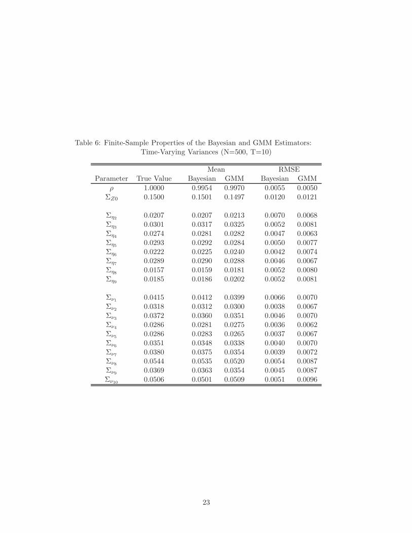
Table 6: Finite-Sample Properties of the Bayesian and GMM Estimators:Time-Varying Variances (N=500, T=10)
Mean RMSEParameter True Value Bayesian GMM Bayesian GMM
ρ 1.0000 0.9954 0.9970 0.0055 0.0050ΣZ0 0.1500 0.1501 0.1497 0.0120 0.0121
Ση2 0.0207 0.0207 0.0213 0.0070 0.0068Ση3 0.0301 0.0317 0.0325 0.0052 0.0081Ση4 0.0274 0.0281 0.0282 0.0047 0.0063Ση5 0.0293 0.0292 0.0284 0.0050 0.0077Ση6 0.0222 0.0225 0.0240 0.0042 0.0074Ση7 0.0289 0.0290 0.0288 0.0046 0.0067Ση8 0.0157 0.0159 0.0181 0.0052 0.0080Ση9 0.0185 0.0186 0.0202 0.0052 0.0081
Σν1 0.0415 0.0412 0.0399 0.0066 0.0070Σν2 0.0318 0.0312 0.0300 0.0038 0.0067Σν3 0.0372 0.0360 0.0351 0.0046 0.0070Σν4 0.0286 0.0281 0.0275 0.0036 0.0062Σν5 0.0286 0.0283 0.0265 0.0037 0.0067Σν6 0.0351 0.0348 0.0338 0.0040 0.0070Σν7 0.0380 0.0375 0.0354 0.0039 0.0072Σν8 0.0544 0.0535 0.0520 0.0054 0.0087Σν9 0.0369 0.0363 0.0354 0.0045 0.0087Σν10 0.0506 0.0501 0.0509 0.0051 0.0096
23

Table 7: Finite-Sample Properties of the Bayesian and GMM Estimators:Labor Income Process with HIP (N=500, T=10)
Parameter True Value Bayesian GMM
ρ 1.0000 0.9936 0.9960(0.0037) (0.0040)[0.0074] [0.0062]
ΣZ0 0.1500 0.1530 0.1538(0.0121) (0.0144)[0.0124] [0.0149]
Ση 0.0200 0.0197 0.0195(0.0021) (0.0045)[0.0021] [0.0045]
Σν 0.0500 0.0498 0.0493(0.0019) (0.0041)[0.0019] [0.0041]
Σβ 0.0004 0.0006 0.0006(0.0003) (0.0005)[0.0003] [0.0005]
*For each parameter and each estimator, the top number is the mean of the estimates across samples, the number in
parentheses is the standard deviation, and the number in square brackets is the root mean square error.
24

Table 8: Finite-Sample Properties of the Bayesian and GMM Estimators:Non-Normal Error Distributions (N=500, T=10)
Parameter True Value Bayesian GMM
ρ 1.0000 0.9960 0.9987(0.0023) (0.0036)[0.0047] [0.0045]
ΣZ0 0.1500 0.1490 0.1492(0.0115) (0.0135)[0.0115] [0.0135]
Ση 0.0200 0.0208 0.0214(0.0014) (0.0024)[0.0016] [0.0028]
Kurtosis of η 8.9743 8.2942 na(1.1551) (na)[1.3354] [na]
hη,1 0.0059 0.0054 nahη,2 0.0766 0.0721 naπη,1 0.8000 0.7560 naπη,2 0.2000 0.2440 na
Σν 0.0500 0.0492 0.0479(0.0023) (0.0035)[0.0025] [0.0042]
Kurtosis of ν 9.0112 9.1119 na(0.5790) (na)[0.5848] [na]
hν,1 0.0146 0.0141 nahν,2 0.1914 0.1902 naπν,1 0.8000 0.7989 naπν,2 0.2000 0.2011 na
*For each parameter and each estimator, the top number is the mean of the estimates across samples, the number in
parentheses is the standard deviation, and the number in square brackets is the root mean square error.
25

A Online Technical Appendix
A.1 Log Likelihood of LGSS
Define the canonical linear Gaussian state space (LGSS) form.
St = AtSt−1 +Btvt
Yt = Ctzt +DtSt + wt
Then the log likelihood of parameter vector θ = (At, Bt, Ct, Dt, Qt, Rt, S0|0, P0|0) is given by:
ln p(Y T |θ)
= lnT∏
t=1
p(Yt|Yt−1, θ)
=
T∑
t=1
ln p(Yt|Yt−1, θ)
=
T∑
t=1
ln[(2π)−0.5kdet[P−0.5t|t−1
]exp[−0.5(Yt − Ctzt −DtSt|t−1)′P−1
t|t−1(Yt − Ctzt −DtSt|t−1)]]
=
T∑
t=1
ln[(2π)−0.5kdetP−0.5t|t−1
] +
T∑
t=1
ln[exp[−0.5(Yt − Ctzt −DtSt|t−1)′P−1
t|t−1(Yt − Ctzt −DtSt|t−1)]]
= −0.5Tk ln(2π)− 0.5T∑
t=1
ln[detPt|t−1] +T∑
t=1
[−0.5(Yt − Ctzt −DtSt|t−1)′P−1
t|t−1(Yt − Ctzt −DtSt|t−1)]
A.2 Bayesian Estimation Procedure
The labor income process we want to estimate is:
yi,t = Xi,tβ + ǫi,t +Σ0.5ν νi,t
ǫi,t = ρǫi,t−1 +Σ0.5η ηi,t
for i = 1, ..., N and t = 1, ..., T . ηi,t and νi,t are independent across i and t, and are distributed asstandard normal:
ηi,t ∼ N(0, 1)
and
νi,t ∼ N(0, 1)
ǫi,0 is also distributed as normal:
ǫi,0 ∼ N (0,ΣZ0)
Xi,t consists of a polynomial of age, race, education, urban residence controls, etc.
Our goal is to draw from p(
β, ρ,Ση,Σν ,ΣZ0, {ǫi,t}t=0,Ti=1,N |{yi,t}
t=1,Ti=1,N
)
.
26

A.2.1 Prior Distribution
We specify the prior distributions for β and ρ to be normal with arbitrarily large variances, truncatingρ ∈ [0, 1] to ensure stationarity.
β ∼ N (β0,Γ0,β)
ρ ∼ N (ρ0,Γ0,ρ) I[−1 ≤ ρ ≤ 1]
We specify the prior distributions for Ση, Σν , and ΣZ0 to be inverse-gamma.
Ση ∼ IG(
T0,η, S−1
0,η
)
Σν ∼ IG(
T0,ν, S−1
0,ν
)
ΣZ0 ∼ IG(
T0,Z0, S−1
0,Z0
)
A.2.2 Gibbs Sampling
We use Gibbs sampling with the following 6 blocks.
Block 1 : p(
β|ρ,Ση,Σν ,ΣZ0, {ǫi,t}t=0,Ti=1,N , {yi,t}
t=1,Ti=1,N
)
Block 2 : p(
ρ|β,Ση,Σν ,ΣZ0, {ǫi,t}t=0,Ti=1,N , {yi,t}
t=1,Ti=1,N
)
Block 3 : p(
Ση|β, ρ,Σν ,ΣZ0, {ǫi,t}t=0,Ti=1,N , {yi,t}
t=1,Ti=1,N
)
Block 4 : p(
Σν |β, ρ,Ση,ΣZ0, {ǫi,t}t=0,Ti=1,N , {yi,t}
t=1,Ti=1,N
)
Block 5 : p(
ΣZ0|β, ρ,Ση,Σν , {ǫi,t}t=0,Ti=1,N , {yi,t}
t=1,Ti=1,N
)
Block 6 : p(
{ǫi,t}t=0,Ti=1,N |β, ρ,Ση,Σν ,ΣZ0, {yi,t}
t=1,Ti=1,N
)
Throughout Block 1 to Block 4, the formulae are the same as in the standard case with one person,except that we have T*N observations, instead of T observations.
Block 1: β
It is identical to the problem of drawing from the posterior of coefficients in a linear regression model. Theposterior distribution is normal, and its mean and variance are analytically computed (see Chapter 2 ofGeweke (2005)).
p(
β|ρ,Ση,Σν ,ΣZ0, {ǫi,t}t=0,Ti=1,N , {yi,t}
t=1,Ti=1,N
)
∼ N (µ1,β ,Γ1,β)
where27
27In the case of an informative prior, the formula is given by
27

Γ1,β = Σν
[
N∑
i=1
T∑
t=1
Xi,tX′i,t
]−1
µ1,β = Γ1,β
[
1
Σν
N∑
i=1
T∑
t=1
Xi,t (yi,t − ǫi,t)′
]
Block 2: ρ
The same as in Block 1, except for truncation (see p.169 of Geweke (2005)).
p(
ρ|β,Ση,Σν ,ΣZ0, {ǫi,t}t=0,Ti=1,N , {yi,t}
t=1,Ti=1,N
)
∼ N (µ1,ρ,Γ1,ρ) [−1 ≤ ρ ≤ 1]
where
Γ1,ρ = Ση
[
N∑
i=1
T∑
t=1
ǫ2i,t−1
]−1
µ1,ρ = Γ1,ρ
[
1
Ση
N∑
i=1
T∑
t=1
ǫi,t−1ǫi,t
]
Block 3: Σν
p(
Σν |β, ρ,Ση,ΣZ0, {ǫi,t}t=0,Ti=1,N , {yi,t}
t=1,Ti=1,N
)
∼ IG(
T1,ν , S−1
1,ν
)
where
T1,ν = T0,ν + TN
S1,ν = S0,ν +
N∑
i=1
T∑
t=1
(yi,t −Xi,tβ − ǫi,t)2
Γ1 =
[
Γ−10 +
1
σ2X
′X
]−1
µ1 = Γ1
[
Γ−10 µ0 +
1
σ2X
′y
]
As Γ0 goes to infinity,
Γ1 → σ2[
X′X]−1
µ1 →
[
X′X]−1 [
X′y]
which coincides with βols and var (βols).
28

Block 4: Ση
p(
Ση|β, ρ,Σν ,ΣZ0, {ǫi,t}t=0,Ti=1,N , {yi,t}
t=1,Ti=1,N
)
∼ IG(
T1,η, S−1
1,η
)
where
T1,η = T0,η + TN
S1,η = S0,η +
N∑
i=1
T∑
t=1
(ǫi,t − ρǫi,t−1)2
Block 5: ΣZ0
p(
ΣZ0|β, ρ,Ση,Σν , {ǫi,t}t=0,Ti=1,N , {yi,t}
t=1,Ti=1,N
)
∼ IG(
T1,Z0, S−1
1,Z0
)
where
T1,Z0 = T1,Z0 +N
S1,Z0 = S0,Z0 +
N∑
i=1
ǫ2i,0
Block 6: {ǫt}
For each individual i, we apply the Carter-Kohn algorithm.28
Step 1: Specify S0|0 and P0|0
Step 2: Kalman-FilterStarting from S0|0 and P0|0, compute {Pt|t−1, Pt|t}
Tt=1
and {St|t}Tt=1
using the Kalman Filter.
St|t−1 = AtSt−1|t−1
Pt|t−1 = AtPt−1|t−1A′t +BQtB
′
Gt = DtPt|t−1D′t +Rt
Kt = Pt|t−1D′tG
−1
t
St|t = St|t−1 +Kt(Yt − Ctzt −DtSt|t−1)
Pt|t = (Ins−KtDt)Pt|t−1
where Ss|t ≡ E [Ss|Yt] and Ps|t ≡ V ar [Ss|Y
t].
Step 3: Carter-Kohn’s backward recursion:At each t=T through 1 going backward, compute
St−1|t = St−1|t−1 + Pt−1|t−1A′tP
−1
t|t−1(St −AtSt−1|t−1)
Pt−1|t = Pt−1|t−1 − Pt−1|t−1A′tP
−1
t|t−1AtPt−1|t−1
28For details see Carter and Kohn (1994).
29

based on St, and draw St−1 from N(
St−1|t, Pt−1|t
)
.
A.3 Bayesian Estimation Procedure with Missing Data
This section presents how to modify Gibbs Block 6 to handle missing observations. In terms of estimation,unbalanced panel datasets can be seen as containing systematic missing observations and does not introduceextra complication.
The LGSS with missing observations can be written as
St = AtSt−1 +Bvt
Yt = Ctzt +DtSt + wt
where
vt ∼ N (0, Qt)
wt ∼ N (0, Rt)
S0 ∼ N(
S0|0, P0|0
)
When working with missing data, it is convenient to let Yt denote a vector containing the incomes ofmultiple individuals at time t.29 Note that some elements of Yt may be missing, i.e., Yi,t = ‘NaN ′. Let nm,t
be the number of missing observations at time t. Let Wt be a (ny − nm,t)− by − ny matrix that selects theelements of Yt that are not missing. For example, suppose Yt is 6-by-1, and the second and fourth elementsare missing.
Yt =
3.5‘NaN ′
2.1‘NaN ′
3.25.9
Then, Wt is a 4-by-6 matrix with the following structure.
Wt =
1 0 0 0 0 00 0 1 0 0 00 0 0 0 1 00 0 0 0 0 1
so that
Yt ≡ WtYt =
1 0 0 0 0 00 0 1 0 0 00 0 0 0 1 00 0 0 0 0 1
3.5‘NaN ′
2.1‘NaN ′
3.25.9
=
3.52.13.25.9
When no value is missing, Wt is a ny − by − ny identity matrix, and Yt = Yt.Using this variable Wt, we transform the observation equation for each t to obtain
29In all other sections, Yt refers to the income of a single individual.
30

St = AtSt−1 +Bvt
WtYt = WtCtzt +WtDtSt +Wtwt
Finally, create an indicator variable φt which takes the value 0 when all values of Yt are missing, and 1otherwise. If φt = 0, set Wt = Iny
.
A.3.1 Estimation Algorithm
To modify Block 6: Gibbs Sampling, we must only modify Step 2. Other steps are unmodified.
Step 2: Kalman-FilterStarting from S0|0 and P0|0, compute {Pt|t−1, Pt|t}
Tt=1 and {St|t}
Tt=1 using Kalman Filter.
St|t−1 = AtSt−1|t−1
Pt|t−1 = AtPt−1|t−1A′t +BQtB
′
Gt = WtDtPt|t−1D′tW
′t +WtRtW
′t
Kt = Pt|t−1D′tW
′tG
−1
t
St|t = St|t−1 + φtKt(WtYt −WtCtzt −WtDtSt|t−1)
Pt|t = (Ins−KtWtDt)Pt|t−1
where Ss|t ≡ E [Ss|Yt] and Ps|t ≡ V ar [Ss|Y
t]. In case where all values of Yt are missing, simply set
St|t−1 = AtSt−1|t−1
Pt|t−1 = AtPt−1|t−1A′t +BQtB
′
St|t = St|t−1
Pt|t = Pt|t−1
A.4 Bayesian Estimation Procedure with Heterogeneous Income Profiles
The labor income process we want to estimate is:
yi,t = Xi,tβi + ǫi,t +Σ0.5ν νi,t
ǫi,t = ρǫi,t−1 +Σ0.5η ηi,t
for i = 1, ..., N and t = 1, ..., T . ηi,t and νi,t are independent across i and t, and are distributed asstandard normal. ǫi,0 is distributed as normal with variance ΣZ0. For each i, βi is distributed as mean zeroand variance Σβ :
βi ∼ N (0,Σβ)
Xi,t consists of a polynomial of age, race, education, urban residence controls, etc. We use βN to denote
{βi}Ni=1
. Our goal is to draw from p(
βN , ρ,Ση,Σν ,ΣZ0, {ǫi,t}t=0,Ti=1,N |{yi,t}
t=1,Ti=1,N
)
.
31

A.4.1 Prior Distribution
Select the prior distribution for ρ to be normal and the distributions for Ση, Σν , and ΣZ0 to be inverse-gamma. We specify the prior distributions for Σβ to be inverse-gamma.
Σβ ∼ IG(
T0,β, S−1
0,β
)
A.4.2 Gibbs Sampling
We use Gibbs sampling with the following 7 blocks.
Block 1 : p(
βN |ρ,Σβ ,Ση,Σν ,ΣZ0, {ǫi,t}t=0,Ti=1,N , {yi,t}
t=1,Ti=1,N
)
Block 2 : p(
Σβ |ρ, βN ,Ση,Σν ,ΣZ0, {ǫi,t}
t=0,Ti=1,N , {yi,t}
t=1,Ti=1,N
)
Block 3 : p(
ρ|βN ,Σβ ,Ση,Σν ,ΣZ0, {ǫi,t}t=0,Ti=1,N , {yi,t}
t=1,Ti=1,N
)
Block 4 : p(
Ση|βN , ρ,Σβ,Σν ,ΣZ0, {ǫi,t}
t=0,Ti=1,N , {yi,t}
t=1,Ti=1,N
)
Block 5 : p(
Σν |βN , ρ,Σβ,Ση,ΣZ0, {ǫi,t}
t=0,Ti=1,N , {yi,t}
t=1,Ti=1,N
)
Block 6 : p(
ΣZ0|βN , ρ,Σβ,Ση,Σν , {ǫi,t}
t=0,Ti=1,N , {yi,t}
t=1,Ti=1,N
)
Block 7 : p(
{ǫi,t}t=0,Ti=1,N |βN ,Σβ, ρ,Ση,Σν ,ΣZ0, {yi,t}
t=1,Ti=1,N
)
Modification of Blocks 3–7 are straightforward. We focus on block 1 and 2.
Block 1: βN
As in the previous case, the posterior is normally distributed. However, we now need to compute the posteriormean and variance for each individual.
p(
βi|ρ,Ση,Σν ,ΣZ0,Σβ , {ǫi,t}t=0,Ti=1,N , {yi,t}
t=1,Ti=1,N
)
∼ N (µi,1,β,Γi,1,β)
where
Γi,1,β =
[
Σ−1
β +1
Σν
X ′iXi
]−1
µi,1,β = Γi,1,β
[
1
Σν
X ′i (yi − ǫi)
]
Block 2: Σβ
p(
Σβ |βN , ρ,Ση,Σν ,ΣZ0, {ǫi,t}
t=1,Ti=0,N , {yi,t}
t=1,Ti=1,N
)
∼ IG(
T1,β, S−1
1,β
)
where
32

T1,β = T0,β +N
S1,β = S0,β +
N∑
i=1
(βi)2
A.5 Bayesian Estimation Procedure with a Mixture of Normal Distributions
The labor income process we want to estimate is:
yi,t = Xi,tβ + ǫi,t + νi,t
ǫi,t = ρǫi,t−1 + ηi,t
for i = 1, ..., N and t = 1, ..., T .
ηi,t and νi,t are independent across i and t. They are distributed according to a mixture of mη and mν
number of normals, respectively.
ηi,t|sη,i,t=j ∼ N(
0, hηhjη
)
p (sη,i,t = j) = πjη ∀j ∈ 1, 2, ...,mη
νi,t|sν,i,t=j ∼ N(
0, hνhjν
)
p (sν,i,t = j) = πjν ∀j ∈ 1, 2, ...,mν
For the shock k ∈ {η, ν}, hkhjk is the variance of distribution j, and π
jk is the probability weight for
distribution j.3031 sk,i,t indicates from which distribution of the mixture the innovation for individual i intime t came.
As before, ǫi,0 is distributed as normal:
ǫi,0 ∼ N (0,ΣZ0)
Our goal is to draw from
p(
β, ρ, hν , {hjν}
mν
j=1, {πj
ν}mν
j=1, {sν,i,t}
t=1,Ti=1,N , hη, {h
jη}
mη
j=1, {πj
η}mη
j=1, {sη,i,t}
t=1,Ti=1,N ,ΣZ0, {ǫi,t}
t=0,Ti=1,N |{yi,t}
t=1,Ti=1,N
)
A.5.1 Prior
We specify the prior for β and ρ to be normal with arbitrarily large variance.
30Note: h and hj are not identified separately. Since we are only interested in h times hj the lack of identificationis inconsequential. h is added for numerical/computational reasons. See Gelman, Carlin, Stern, and Rubin (2009).
31The likelihood function of the mixture model is invariant to permutation of the components of the mixture. Inour application, we simply label the component with a smaller variance as the first component and the componentwith a larger variance as the second component. For more detailed discussions, see Geweke (2007).
33

β ∼ N (β0,Γ0,β)
ρ ∼ N (ρ0,Γ0,ρ) I [−1 ≤ ρ ≤ 1]
We specify the prior for ΣZ0, hν , {hjν}
mν
j=1, hη, and {hj
η}mη
j=1to be inverse-gamma.
ΣZ0 ∼ IG(
T0,Z0, S−1
0,Z0
)
hν ∼ IG(
Thν ,0, S−1
hν ,0
)
hjν ∼ IG
(
Thjν ,0
, S−1
hjν ,0
)
hη ∼ IG(
Thη,0, S−1
hη,0
)
hjη ∼ IG
(
Thjη,0
, S−1
hjη,0
)
We specify the prior for {πjν}
mν
j=1and {πj
η}mη
j=1to be Dirichlet.
p(
{πjη}
mη
j=1
)
∼ D (r, r, ..., r)
p(
{πjν}
mν
j=1
)
∼ D (r, r, ..., r)
In the estimation of the model with two normal mixtures in Section 4.4, the true value for hη and hν
are set to one. For prior distributions, we set Thν ,0 = Th1ν ,0
= Th2ν ,0
= 2, Shν ,0 = 1, Sh1ν ,0
= Sh2ν ,0
= 0.01,Thη,0 = Th1
η,0= Th2
η,0= 2, Shη,0 = 1, Sh1
η ,0= Sh2
η,0= 0.01. For the parameter of the Dirichlet distribution,
we set r = 0.5 for both πη and πν .
A.5.2 Estimation Algorithm
Gibbs sampling consists of the following 6 main blocks:Block 1:
p(
β|ρ, hν , {hjν}
mν
j=1, {πj
ν}mν
j=1, {sν,i,t}
t=1,Ti=1,N , hη, {h
jη}
mη
j=1, {πj
η}mη
j=1, {sη,i,t}
t=1,Ti=1,N ,ΣZ0, {ǫi,t}
t=0,Ti=1,N , {yi,t}
t=1,Ti=1,N
)
Block 2:
p(
ρ|β, hν , {hjν}
mν
j=1, {πj
ν}mν
j=1, {sν,i,t}
t=1,Ti=1,N , hη, {h
jη}
mη
j=1, {πj
η}mη
j=1, {sη,i,t}
t=1,Ti=1,N ,ΣZ0, {ǫi,t}
t=0,Ti=1,N , {yi,t}
t=1,Ti=1,N
)
Block 3.1:
p(
hν |β, ρ, {hjν}
mν
j=1, {πj
ν}mν
j=1, {sν,i,t}
t=1,Ti=1,N , hη, {h
jη}
mη
j=1, {πj
η}mη
j=1, {sη,i,t}
t=1,Ti=1,N ,ΣZ0, {ǫi,t}
t=0,Ti=1,N , {yi,t}
t=1,Ti=1,N
)
Block 3.2:
p(
{hjν}
mν
j=1|β, ρ, hν , {π
jν}
mν
j=1, {sν,i,t}
t=1,Ti=1,N , hη, {h
jη}
mη
j=1, {πj
η}mη
j=1, {sη,i,t}
t=1,Ti=1,N ,ΣZ0, {ǫi,t}
t=0,Ti=1,N , {yi,t}
t=1,Ti=1,N
)
Block 3.3:
p(
{πjν}
mν
j=1|β, ρ, hν , {h
jν}
mν
j=1, {sν,i,t}
t=1,Ti=1,N , hη, {h
jη}
mη
j=1, {πj
η}mη
j=1, {sη,i,t}
t=1,Ti=1,N ,ΣZ0, {ǫi,t}
t=0,Ti=1,N , {yi,t}
t=1,Ti=1,N
)
34
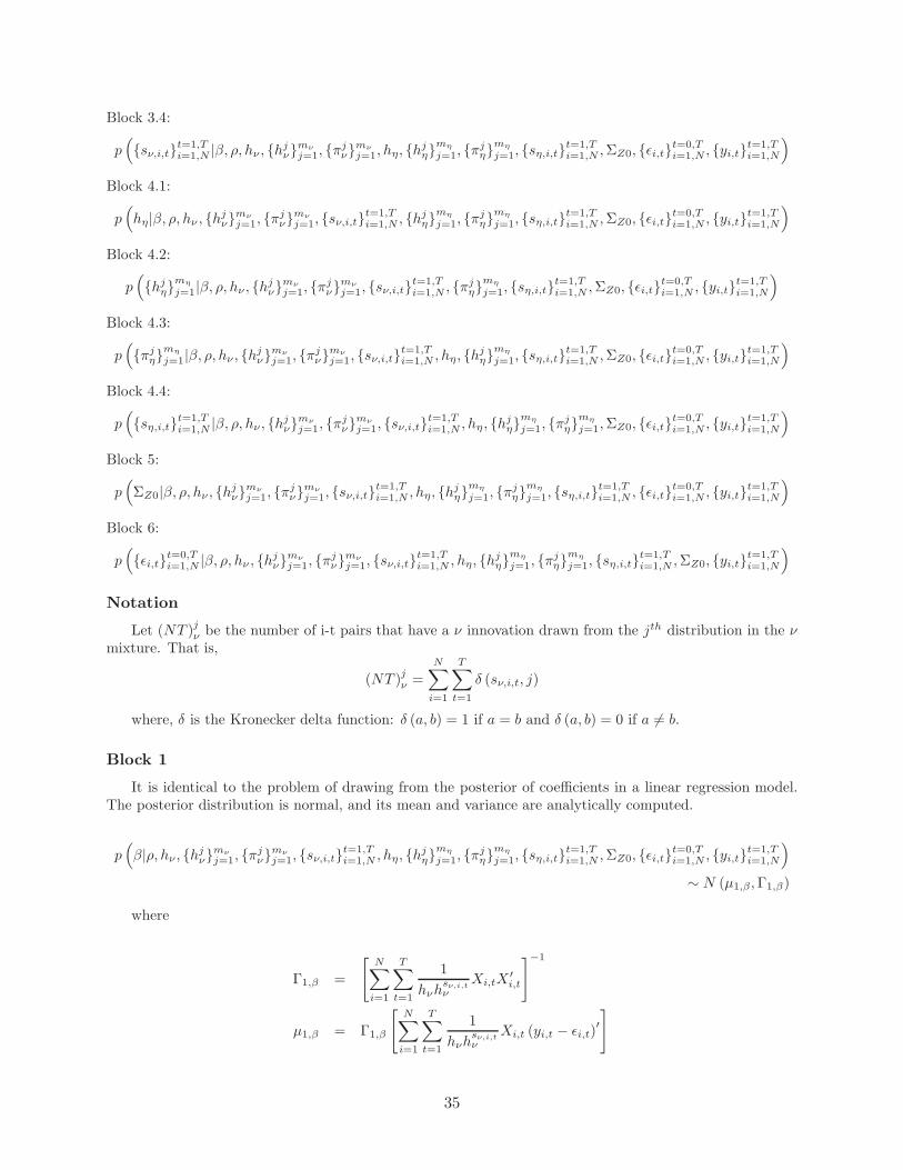
Block 3.4:
p(
{sν,i,t}t=1,Ti=1,N |β, ρ, hν , {h
jν}
mν
j=1, {πj
ν}mν
j=1, hη, {h
jη}
mη
j=1, {πj
η}mη
j=1, {sη,i,t}
t=1,Ti=1,N ,ΣZ0, {ǫi,t}
t=0,Ti=1,N , {yi,t}
t=1,Ti=1,N
)
Block 4.1:
p(
hη|β, ρ, hν , {hjν}
mν
j=1, {πj
ν}mν
j=1, {sν,i,t}
t=1,Ti=1,N , {hj
η}mη
j=1, {πj
η}mη
j=1, {sη,i,t}
t=1,Ti=1,N ,ΣZ0, {ǫi,t}
t=0,Ti=1,N , {yi,t}
t=1,Ti=1,N
)
Block 4.2:
p(
{hjη}
mη
j=1|β, ρ, hν , {h
jν}
mν
j=1, {πj
ν}mν
j=1, {sν,i,t}
t=1,Ti=1,N , {πj
η}mη
j=1, {sη,i,t}
t=1,Ti=1,N ,ΣZ0, {ǫi,t}
t=0,Ti=1,N , {yi,t}
t=1,Ti=1,N
)
Block 4.3:
p(
{πjη}
mη
j=1|β, ρ, hν , {h
jν}
mν
j=1, {πj
ν}mν
j=1, {sν,i,t}
t=1,Ti=1,N , hη, {h
jη}
mη
j=1, {sη,i,t}
t=1,Ti=1,N ,ΣZ0, {ǫi,t}
t=0,Ti=1,N , {yi,t}
t=1,Ti=1,N
)
Block 4.4:
p(
{sη,i,t}t=1,Ti=1,N |β, ρ, hν , {h
jν}
mν
j=1, {πj
ν}mν
j=1, {sν,i,t}
t=1,Ti=1,N , hη, {h
jη}
mη
j=1, {πj
η}mη
j=1,ΣZ0, {ǫi,t}
t=0,Ti=1,N , {yi,t}
t=1,Ti=1,N
)
Block 5:
p(
ΣZ0|β, ρ, hν , {hjν}
mν
j=1, {πj
ν}mν
j=1, {sν,i,t}
t=1,Ti=1,N , hη, {h
jη}
mη
j=1, {πj
η}mη
j=1, {sη,i,t}
t=1,Ti=1,N , {ǫi,t}
t=0,Ti=1,N , {yi,t}
t=1,Ti=1,N
)
Block 6:
p(
{ǫi,t}t=0,Ti=1,N |β, ρ, hν , {h
jν}
mν
j=1, {πj
ν}mν
j=1, {sν,i,t}
t=1,Ti=1,N , hη, {h
jη}
mη
j=1, {πj
η}mη
j=1, {sη,i,t}
t=1,Ti=1,N ,ΣZ0, {yi,t}
t=1,Ti=1,N
)
Notation
Let (NT )jν be the number of i-t pairs that have a ν innovation drawn from the jth distribution in the ν
mixture. That is,
(NT )j
ν =
N∑
i=1
T∑
t=1
δ (sν,i,t, j)
where, δ is the Kronecker delta function: δ (a, b) = 1 if a = b and δ (a, b) = 0 if a 6= b.
Block 1
It is identical to the problem of drawing from the posterior of coefficients in a linear regression model.The posterior distribution is normal, and its mean and variance are analytically computed.
p(
β|ρ, hν , {hjν}
mν
j=1, {πj
ν}mν
j=1, {sν,i,t}
t=1,Ti=1,N , hη, {h
jη}
mη
j=1, {πj
η}mη
j=1, {sη,i,t}
t=1,Ti=1,N ,ΣZ0, {ǫi,t}
t=0,Ti=1,N , {yi,t}
t=1,Ti=1,N
)
∼ N (µ1,β,Γ1,β)
where
Γ1,β =
[
N∑
i=1
T∑
t=1
1
hνhsν,i,tν
Xi,tX′i,t
]−1
µ1,β = Γ1,β
[
N∑
i=1
T∑
t=1
1
hνhsν,i,tν
Xi,t (yi,t − ǫi,t)′
]
35

Block 2
p(
ρ|β, hν , {hjν}
mν
j=1, {πj
ν}mν
j=1, {sν,i,t}
t=1,Ti=1,N , hη, {h
jη}
mη
j=1, {πj
η}mη
j=1, {sη,i,t}
t=1,Ti=1,N ,ΣZ0, {ǫi,t}
t=0,Ti=1,N , {yi,t}
t=1,Ti=1,N
)
∼ N (µ1,ρ,Γ1,ρ) [−1 ≤ ρ ≤ 1]
where
Γ1,ρ =
[
N∑
i=1
T∑
t=1
1
hηhsη,i,t
ν
ǫ2i,t−1
]−1
µ1,ρ = Γ1,ρ
[
N∑
i=1
T∑
t=1
1
hνhsν,i,tν
ǫi,t−1ǫi,t
]
Block 3.1
p(
hν |β, ρ, {hjν}
mν
j=1, {πj
ν}mν
j=1, {sν,i,t}
t=1,Ti=1,N , hη, {h
jη}
mη
j=1, {πj
η}mν
j=1, {sη,i,t}
t=1,Ti=1,N ,ΣZ0, {ǫi,t}
t=0,Ti=1,N , {yi,t}
t=1,Ti=1,N
)
∼ IG(
S−1
hν ,1, Thν ,1
)
where
Thν ,1 = Thν ,0 +mν +NT
Shν ,1 = Shν ,0 +N∑
i=1
T∑
t=1
1
hsν,i,tν
(yi,t −Xi,tβ − ǫi,t)2
Block 3.2
p(
{hjν}
mν
j=1|β, ρ, hν , {π
jν}
mν
j=1, {sν,i,t}
t=1,Ti=1,N , hη, {h
jη}
mη
j=1, {πj
η}mν
j=1, {sη,i,t}
t=1,Ti=1,N ,ΣZ0, {ǫi,t}
t=0,Ti=1,N , {yi,t}
t=1,Ti=1,N
)
∼ IG(
S−1
hjν ,1
, Thjν ,1
)
where
Thjν ,1
= Tjν,0 + (NT )
j
ν
Shjν ,1
= Shjν ,0
+1
hν
N∑
i=1
T∑
t=1
δ (sν,i,t, j) (yi,t −Xi,tβ − ǫi,t)2
for all 1 ≤ j ≤ mν .
36

Block 3.3
p(
{πjν}
mν
j=1|β, ρ, hν , {h
jν}
mν
j=1, {sν,i,t}
t=1,Ti=1,N , hη, {h
jη}
mη
j=1, {πj
η}mν
j=1, {sη,i,t}
t=1,Ti=1,N ,ΣZ0, {ǫi,t}
t=0,Ti=1,N , {yi,t}
t=1,Ti=1,N
)
∼ D (bν,1, bν,2, ..., bν,mν)
where
bν,j = r + (NT )jν
for all 1 ≤ j ≤ mν .
Block 3.4
p(
sν,i,t = j|β, ρ, hν , {hjν}
mν
j=1, {πj
ν}mν
j=1, hη, {h
jη}
mη
j=1, {πj
η}mν
j=1, {sη,i,t}
t=1,Ti=1,N ,ΣZ0, {ǫi,t}
t=0,Ti=1,N , {yi,t}
t=1,Ti=1,N
)
∼ πjν
(
hjν
)−0.5exp
[
−(yi,t −Xi,tβ − ǫi,t)
2
2hνhjν
]
for all 1 ≤ t ≤ T , 1 ≤ i ≤ N .
Block 4
This block is analogous to Block 3. Replace each ν subscript with η and yi,t−Xi,tβ−ǫi,t with ǫi,t−ρǫi,t−1.
Block 5
p(
ΣZ0|β, ρ, hν , {hjν}
mν
j=1, {πj
ν}mν
j=1, {sν,i,t}
t=1,Ti=1,N , hη, {h
jη}
mη
j=1, {πj
η}mη
j=1, {sη,i,t}
t=1,Ti=1,N , {ǫi,t}
t=0,Ti=1,N , {yi,t}
t=1,Ti=1,N
)
∼ IG(
T1,Z0, S−1
1,Z0
)
where
T1,Z0 = T1,Z0 +N
S1,Z0 = S0,Z0 +N∑
i=1
ǫ2i,0
Block 6
For each individual i, we apply the Carter-Kohn algorithm. To cast our labor income processes into ourcanonical form,
At = ρ, Bt = 1, Ct = β,
Dt = 1, Qt = hηhsη,i,t
η , Rt = hνhsν,i,tν ,
zt = Xi,t, S0|0 = 0, P0|0 = ΣZ0
37