Small Open Economy

Lawrence ChristianoMarch, 2014, Bank of Korea

Department of Economics, Northwestern University

Outline

Simple Closed Economy Model

Extend Model to Open EconomyI Equilibrium conditionsI Indicate complications to bring the model to the data.I Similar in spirit to Ramses I model

F Adolfson-Laséen-Lindé-Villan at Swedish Riksbank

Brief Discussion of Introducing Financial FrictionsI Christiano-Trabandt-Walentin (CTW) Model, Ramses II model.

F Based on Christiano-Motto-Rostagno (‘Risk Shocks’)

I Mihai Copaciu of Romanian Central Bank.

Application:I will US ‘lift o§’ act like a locomotive to rest of world economy, or willit be a problem (especially for EME’s)?

Simple Closed Economy Model

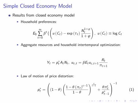
Results from closed economy modelI Household preferences:

E0•

Ât=0

bt{

u (Ct )− exp (tt )

N1+jt1+ j

!, u (Ct ) ≡ logCt

I Aggregate resources and household intertemporal optimization:

Yt = p∗t AtNt , uc ,t = bEtuc ,t+1Rt

pt+1

I Law of motion of price distortion:

p∗t =

0

@(1− q)

1− q (pt )

#−1

1− q

! ##−1

+qp#

tp∗t−1

1

A−1

(1)

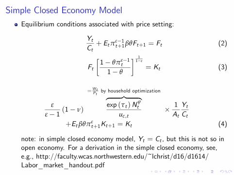
Simple Closed Economy ModelEquilibrium conditions associated with price setting:

YtCt+ Etp#−1

t+1bqFt+1 = Ft (2)

Ft

'1− qp#−1

t

1− q

( 11−#

= Kt (3)

#

#− 1(1− n)

=WtPt

by household optimizationz }| {exp (tt )N

jt

uc ,t×1At

YtCt

+Etbqp#t+1Kt+1 = Kt (4)

note: in simple closed economy model, Yt = Ct , but this is not so inopen economy. For a derivation in the simple closed economy, see,e.g., http://faculty.wcas.northwestern.edu/~lchrist/d16/d1614/Labor_market_handout.pdf

Extensions to Small Open Economy

Outline:I the equilibrium conditions of the open economy modelI system jumps from 6 equations in basic model to 16 equations in 16variables!

Extensions to Small Open Economy: 16 variables

rate of depreciation, exports, real foreign assets, terms of trade, real exchange ratez }| {st , xt , aft , p

xt , qt

price of domestic consumption (now, c is a composite of domestically produced goods & imports)z}|{pct

price of importsz}|{pmt

consumption price inflationz}|{pct

reduced form object to (i) achieve technical objective, (ii) adjust UIP implicationz}|{Ft

closed economy variablesz }| {Rt ,pt ,Nt , ct ,Kt ,Ft , p∗t

Extensions to Small Open Economy- Outline

After describing 16 equilibrium conditions:I compute the steady stateI the ‘uncovered interest parity puzzle’, and the role of Ft in addressingthe puzzle.

I summary of the endogenous and exogenous variables of the model, aswell as the equations.

I several computational experiments to illustrate the properties of themodel.

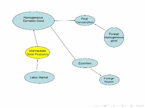
Modifications to Simple Model to Create Open Economy

Unchanged:I household preferencesI production of (domestic) homogeneous good, Yt (= Atp∗t Nt )I three Calvo price friction equations

Changes:I household budget constraint includes opportunity to acquire foreignassets/liabilities.

I intertemporal Euler equation changed as a reduced formaccommodation of evidence on uncovered interest parity.

I Yt = Ct no longer true.I introduce exports, imports, balance of payments.I exchange rate,

St = domestic currency price of one unit of foreign currencySt =

domestic moneyforeign money

Monetary Policy: two approaches

Taylor rule

log-RtR

.= rR log

-Rt−1R

.+ (1− rR )Et [rp log

-pct+1pc

.(5)

+ry log-yt+1y

.] + #R ,t

where (could also add exchange rate, real exchange rate and otherthings):

pc ~target consumer price inflation

#R ,t ~iid, mean zero monetary policy shock

yt ~Yt/AtRt ~‘risk free’ nominal rate of interest

#R ,t ~mean zero monetary policy shock.

Monetary Policy: two approaches

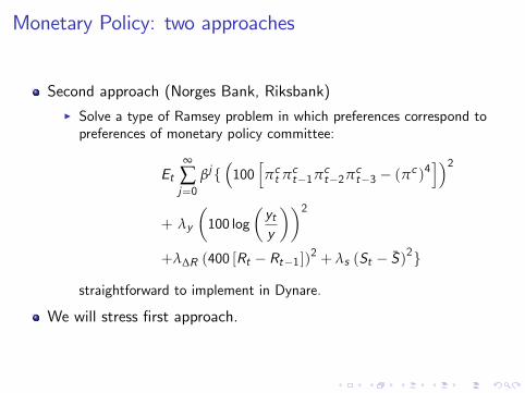
Second approach (Norges Bank, Riksbank)I Solve a type of Ramsey problem in which preferences correspond topreferences of monetary policy committee:

Et•

Âj=0

bj{/100

hpct pct−1pct−2pct−3 − (p

c )4i22

+ ly

-100 log

-yty

..2

+lDR (400 [Rt − Rt−1 ])2 + ls (St − S)

2}

straightforward to implement in Dynare.

We will stress first approach.

Household Budget Constraint

‘Uses of funds less than or equal to sources of funds’

StAft+1 + PtCt + Bt+1

≤ BtRt−1 + SthFt−1Rft−1

iAft +WtNt + transfers and profitst

Domestic bonds

Bt ~beginning of period t stock of loans

Rt ~rate of return on bonds

Foreign assets

Aft ~beginning-of-period t net stock of foreign assets

(liabilities, if negative) held by domestic residents.

FtRft ~rate of return on Aft

Ft ~premium on foreign asset returns

Household Intertemporal First Order Conditions: ForeignAssets

Optimality of foreign asset choice (verify this by solving Lagrangianrepresentation of household problem)

utility cost of 1 unit of foreign currency=St units of domestic currency, St/Pct units of Ctz }| {uc ,tStPct

= bEt

conversion into utility unitsz }| {uc ,t+1

×

quantity of domestic cons. goods purchased from the payo§ of 1 unit of foreign currencyz }| {

St+1

foreign currency payo§ next period from one unit of foreign currency todayz }| {Rft Ft

Pct+1

Household Intertemporal First Order Conditions: ForeignAssets

First order condition:

StPct Ct

= bEtSt+1Rft Ft

Pct+1Ct+1

Scaling:

1ct= bEt

st+1Rft Ft

pct+1ct+1 exp (Dat+1), st ≡

StSt−1

, ct =CtAt. (6)

Technology:at ≡ log (At ) , Dat = at − at−1.

Household Intertemporal First Order Conditions: DomesticAssets

First order condition:

1Pct Ct

= bEtRt

Pct+1Ct+1

Scaling:1ct= bEt

Rtpct+1ct+1 exp (Dat+1)

. (7)

Final Domestic Consumption Goods

Produced by representative, competitive firm using:

Ct =

"

(1−wc )1

hc

/Cdt2 hc−1

hc +w1

hcc (Cmt )

hc−1hc

# hchc−1

where

Cdt ~ domestic homogeneous output good, price PtCmt ~ imported good, price Pmt

5≡ StPft

6

Ct ~ final consumption good, Pcthc ~ elasticity of substitution, domestic and foreign goods.

Final Domestic Consumption Goods

Profit maximization by representative firm:

maxPct Ct − Pmt C

mt − PtC

dt ,

subject to production function.

First order conditions associated with maximization:

Cmt : Pct

=/

wcCtCmt

2 1hc

z }| {dCtdCmt

= Pmt , Cdt : Pct

=

-(1−wc )

CtCdt

. 1hc

z}|{dCtdCdt

= Pt

so that the demand functions are:

Cmt = wc

-PctPmt

.hcCt , Cdt = (1−wc )

-PctPt

.hcCt .

Price Function

Substituting demand functions back into the production function:

Ct = [(1−wc )1

hc

-Ct

-PctPt

.hc(1−wc )

. hc−1hc

+w1

hcc

-wc

-PctPmt

.hcCt

. hc−1hc

]hc

hc−1 ,

or

pct =h(1−wc ) +wc (pmt )

1−hci 11−hc

,(8)

where

pct ≡PctPt, pmt ≡

PmtPt.

Real Exchange Rate and Consumption Price Inflation

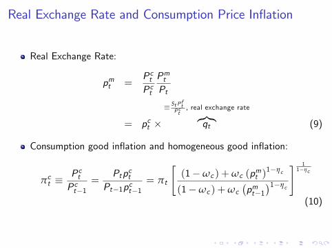
Real Exchange Rate:

pmt =PctPct

PmtPt

= pct ×

≡ St Pft

Pct, real exchange ratez}|{qt (9)

Consumption good inflation and homogeneous good inflation:

pct ≡PctPct−1

=Ptpct

Pt−1pct−1= pt

"(1−wc ) +wc (pmt )

1−hc

(1−wc ) +wc5pmt−1

61−hc

# 11−hc

(10)

Exports

Foreign demand for domestic goods:

Xt =-PxtPft

.−hfY ft = (p

xt )−hf Y ft ,

terms of tradez}|{pxt =

PxtPft

Y ft ~ foreign outputPft ~ foreign currency price of foreign goodPxt ~ foreign currency price of export good

Scaling by Atxt = (pxt )

−hf y ft (11)

Rate of Depreciation, Inflation...

Competition: Price of export equals marginal cost:

StPxt = Pt .

Scaling:

1 =StPxtPt

=Pct StP

ft P

xt

PtPct Pft

= qtpxt pct (12)

Also,

qtqt−1

= stpftpct, st ≡

StSt−1

, pft ≡PftPft−1

(13)

Homogeneous Goods Market Clearing

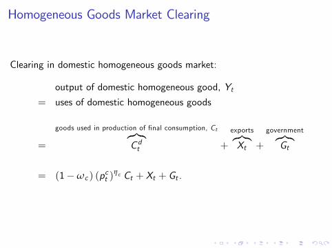
Clearing in domestic homogeneous goods market:

output of domestic homogeneous good, Yt= uses of domestic homogeneous goods

=

goods used in production of final consumption, Ctz}|{Cdt +

exportsz}|{Xt +

governmentz}|{Gt

= (1−wc ) (pct )hc Ct + Xt + Gt .

Aggregate Employment and Uses of Homogeneous Goods

Substituting out in previous expression for Yt :

Atp∗t Nt = (1−wc ) (pct )hc Ct + Xt + Gt ,

or,p∗t Nt = (1−wc ) (pct )

hc ct + xt + gt , (14)

ct ≡CtAt, xt ≡

XtAt, gt ≡

GtAt.

Balance of Payments

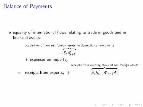
equality of international flows relating to trade in goods and infinancial assets:

acquisition of new net foreign assets, in domestic currency unitsz }| {StAft+1

+ expenses on importst

= receipts from exportst +

receipts from existing stock of net foreign assetsz }| {StRft−1Ft−1Aft

Balance of Payments, the Pieces

Exports and imports:

expenses on importst = StPft wc

-pctpmt

.hc

Ct

receipts from exportst = StPxt Xt .

Balance of payments:

StAft+1 + StPft wc

-pctpmt

.hcCt

= StPxt Xt + StRft−1Ft−1Aft .

Balance of Payments, Scaling

Scaling by PtAt :

StAft+1PtAt

+StPftPt

wc

-pctpmt

.hcct

=StPxtPt

xt +StRft−1Ft−1Aft

PtAt,

or,

aft + pmt wc

-pctpmt

.hcct = pct qtp

xt xt +

stRft−1Ft−1aft−1pt exp (Dat )

, (15)

where aft is ‘scaled, homogeneous goods value of net foreign assets’:

aft =StAft+1PtAt

.

Risk Term

Ft = F/aft ,R

ft ,Rt , ft

2= (16)

exp/−fa

/aft − a

2+ fs

/Rt − Rft −

/R − Rf

22+ ft

2

fa > 0, small and not important for dynamics

fs > 0, important

ft ~mean zero, iid.

Discussion of fa.I fa > 0 implies (i) if a

ft > a, then return on foreign assets low and

aft #; (ii) if aft < a, then return on foreign assets high and aft "I implication: fa > 0 is a force that drives a

ft ! a in steady state,

independent of initial conditions.I logic is same as reason why steady state stock of capital in neoclassicalgrowth model is unique, independent of initial conditions.

I in practice, put in a tiny value of fa, so that its only e§ect is to pindown aft in steady state and it does not a§ect dynamics (seeSchmitt-Grohe and Uribe).

Risk Term

Discussion of ft :I Captures, informally, the possibility that there is a shock to therequired return on domestic assets.

F When ft > 0, ‘capital outflow shock’, people stop liking domesticassets

F When ft < 0, ‘safe haven shock’, people love domestic assets (e.g.,Swiss Franc in recent years).

Discussion of fs :I fs reduced form fix for the model.I With fs = 0, model implies Uncovered Interest Parity (UIP), whichdoes not hold in the data.

I to better explain this, it is convenient to first solve for the model’ssteady state.

Steady State

household intertemporal e¢ciency conditions:

1 = bsRf

pc exp (Da)(6)

1 = bR

pc exp (Da)(7)

assumption about foreign households:

pft ≡PftPft−1

(exogenous)

1 = bRf

pf exp (Da)

Steady State

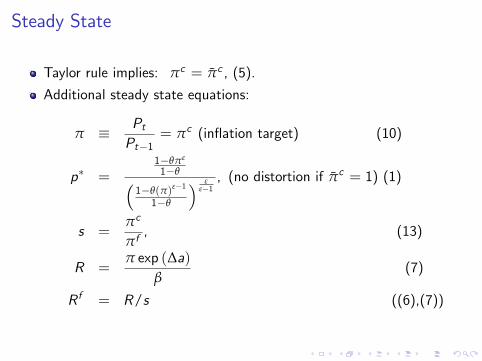
Taylor rule implies: pc = pc , (5).

Additional steady state equations:

p ≡PtPt−1

= pc (inflation target) (10)

p∗ =1−qp#

1−q/1−q(p)#−1

1−q

2 ##−1, (no distortion if pc = 1) (1)

s =pc

pf, (13)

R =p exp (Da)

b(7)

Rf = R/s ((6),(7))

Steady State, Potentially Iterative Part

Rest of the algorithm solves a single non-linear equation in a singleunknown, j.

Set j = pcq

pm = j (9) and px =1j(12)

pc =h(1−wc ) +wc (pm)

1−hci 11−hc (8)

q =j

pc

Steady State, Potentially Iterative Part...Let

g = hg y , a = hay .

Then,

0 = pmwc

-pc

pm

.hcc − pcqpx x −

-sRf

p exp (Da)− 1.

hap∗N (15)

0 = (1−wc ) (pc )hc c + x −

/1− hg

2Np∗ (14)

F =p∗N

c (1− p#−1bq)(2)

K = F'1− qp#−1

1− q

( 11−#

(3)

0 =#

#− 1(1− n)N1+jp∗ + (bqp# − 1)K (4),

These five equations involve the five unknowns: c ,N,F ,K , x . Solvethese. Adjust j until (11) is satisfied. In practice, we simply setj = 1 and used (11) to solve for y f .

Uncovered Interest Parity Algebrasubtract equations (6) and (7):

Et

'Rt − st+1Rft Ft

ct+1pct+1 exp (Dat+1)

(= 0.

I totally di§erent object in square brackets and evaluate in steady state:

dRt − st+1Rft Ft

ct+1pct+1 exp (Dat+1)

=dRt

cpc exp (Da)

−1

cpc exp (Da)

hsRf dFt + sdRft + R

f dst+1i

−R − sRf

[cpc exp (Da)]2d7ct+1pct+1 exp (Dat+1)

8

=1

bc

nRt −

hFt + Rft + st+1

io

wherext ≡ (xt − x) /x = dxt/x .

Uncovered Interest Parity, Linearized RepresentationThen,

Et

'Rt − st+1Rft Ft

ct+1pct+1 exp (Dat+1)

(= 0,

is, to a first approximation,

Et

'1

bc

nRt −

hFt + R ft + st+1

io(= 0

or,Rt = Et st+1 + R ft + Ft .

Conclude, using dxtx ' log (xt/x) , logF = 0 :

logRt − logR = Et [log st+1 − log (s)] + logRft − logRf + logFt

or, using logRf = logR − log s, definition of st+1, rt ≡ logRt ,r ft ≡ logRft

Et log St+1 − log St = rt − r ft + logFt

Uncovered Interest Parity

Under UIP, Ft = 0 :I rt > r ft ! must be an anticipated depreciation (instantaneousappreciation) of the currency for people to be happy holding theexisting stock of net foreign assets

Consider regression relation:

log St+1 − log St = b0 + b1

/rt − r ft

2+ ut .

I Under UIP (and, rational expectations), b0 = 0, b1 = 1.

When Ft 6= 0:

b1 =cov

5log St+1 − log St , rt − r ft

6

var5rt − r ft

6 = 1− fs ,

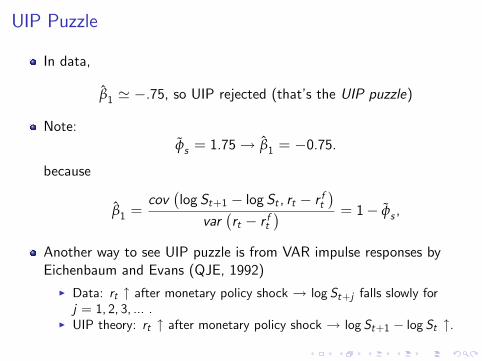
UIP Puzzle

In data,

b1 ' −.75, so UIP rejected (that’s the UIP puzzle)

Note:fs = 1.75! b1 = −0.75.

because

b1 =cov

5log St+1 − log St , rt − r ft

6

var5rt − r ft

6 = 1− fs ,

Another way to see UIP puzzle is from VAR impulse responses byEichenbaum and Evans (QJE, 1992)

I Data: rt " after monetary policy shock ! log St+j falls slowly forj = 1, 2, 3, ... .

I UIP theory: rt " after monetary policy shock ! log St+1 − log St ".

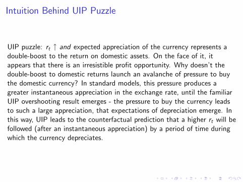
Intuition Behind UIP Puzzle

UIP puzzle: rt " and expected appreciation of the currency represents adouble-boost to the return on domestic assets. On the face of it, itappears that there is an irresistible profit opportunity. Why doesn’t thedouble-boost to domestic returns launch an avalanche of pressure to buythe domestic currency? In standard models, this pressure produces agreater instantaneous appreciation in the exchange rate, until the familiarUIP overshooting result emerges - the pressure to buy the currency leadsto such a large appreciation, that expectations of depreciation emerge. Inthis way, UIP leads to the counterfactual prediction that a higher rt will befollowed (after an instantaneous appreciation) by a period of time duringwhich the currency depreciates.

Intuition Behind ‘Resolution’ of Puzzle

Model’s resolution of the UIP puzzle: when rt " the return required forpeople to hold domestic bonds rises. This is why the double-boost todomestic returns does not create an appetite to buy large amounts ofdomestic assets. Possibly this is a reduced form way to capture the notionthat increases in rt make the domestic economy more risky. (However, theprecise mechanism by which the domestic required return rises - earningson foreign assets go up - may be di¢cult to interpret. An alternativespecification was explored, with risk-premia a§ecting domestic bonds, butthis resulted in indeterminacy problems.)

Dynamics

16 equations: price setting, (1),(2),(3),(4); monetary policy rule, (5);household intertemporal Euler equations (6),(7); relative priceequations (8),(9),(10),(12),(13); aggregate resource condition, (14);balance of payments, (15); risk term, (16); demand for exports (11).

16 endogenous variables: pct , pmt , qt ,Rt ,pt ,p

ct , p

xt ,Nt , p

∗t , a

ft ,Ft ,

st , xt , ct ,Kt ,Ft .

exogenous variables: Rft , yft , ft , gt , #R ,t , Dat , tt , pft .

I for the purpose of numerical calculations, these were modeled asindependent scalar AR(1) processes.

Extensions to Small Open Economy...

the model was solved in the manner described above:- compute the steady state using the formulas described above- log-linearize the 16 equations about steady state- solve the log-linearized system- these calculations were made easy by implementing them in Dynare.

Parameter Values

Numerical examples: Parameter values:

pf = pc = 1.005 fa = 0.03 b = 1.03−1/4

q = 3/4 j = 1 # = 61− n = #−1

# hc = 5 wc = 0.4hg = 0.3 ha = 0 hf = 1.5rR = 0.9 rp = 1.5 ry = 0.15

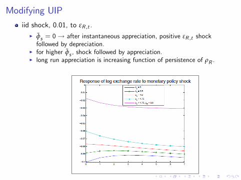
Modifying UIP

iid shock, 0.01, to #R ,t .

I fs = 0! after instantaneous appreciation, positive #R ,t shockfollowed by depreciation.

I for higher fs , shock followed by appreciation.I long run appreciation is increasing function of persistence of rR .

Impact of Modifications to UIP

We now consider a monetary policy shock, #R ,t = 0.01. According to (5), impliesa four percentage point (at an annual rate) policy-induced jump in Rt .The dynamic e§ects are displayed in the following figure, for fs = 0, fs = 1.75

Note: (i) appreciation smaller, though more drawn out, when fs is big; (ii) smaller appreciation results in smaller drop in net

exports, so less of a drop in demand, so less fall in output and inflation; (iii) smaller drop in net exports results in smaller drop in

real foreign assets.

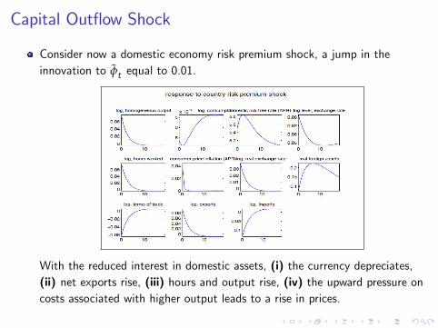
Capital Outflow Shock

Consider now a domestic economy risk premium shock, a jump in theinnovation to ft equal to 0.01.

With the reduced interest in domestic assets, (i) the currency depreciates,(ii) net exports rise, (iii) hours and output rise, (iv) the upward pressure oncosts associated with higher output leads to a rise in prices.

Question Confronting Many Emerging Market Economies..

At some point, the Fed will implement its ‘exit strategy’ and raise USinterest rates (300-350 basis points?).

In the past, when Fed raised rates sharply (e.g., 1982 Volckerdisinflation, 1994 run-up in interest rates), hit the rest of world like abrick:

I Chilean crisis of 1982, Mexican default of August 1982. Mexican crisisof 1994.

Will the US ‘exit strategy’ inflict financial crises around the world,especially in emerging market economies?

I Summer 2013 ‘taper episode’ makes people worry about this possibility.

I’ll call the above possibility the BIS scenario.

BIS Scenario

Low US interest rates since 2008 have encouraged‘excessive’accumulation of debt in the world.

This has particularly a§ected emerging market economies in AsiaandLatin America.

Currency Mismatch Problem May Be Understated..

(Hyun Shin, ‘The Second Phase of Global Liquidity. . . ’, November, 2013)

Many emerging market borrowers issue dollar-denominated debtthrough foreign subsidiaries (say in the UK).

I By the usual definition (based on the residence of the issuer), thebonds are a liability of the UK entity.

But, it’s the consolidated balance sheet that matters to the emergingmarket firm.

I So, the debt issued via a foreign subsidiary could make the emergingmarket firm vulnerable to currency mismatch problems.

Hyun Shin argues:• Amount of dollar denominated debt from emerging market firms may begreatly understated.

• This is suggested by evidence that foreign currency debt by nationalitycan be much larger than foreign debt by the usual residency definition.

Shin conjectures that distinction between external debt according tonationality and residence helps to resolve the ‘taper’ puzzle:

I convulsions in emerging markets during taper episode in summer 2013seem inconsistent with apparently small net external debt position(measured in residence terms) of firms in emerging markets.

Less surprising if external debt position is in fact much bigger.

BIS Scenario

US raises interest rates.

Emerging market exchange rates depreciate.

Financial health of emerging market firms compromised.

They cut back on investment activity. . . .recessions start.

Runs on emerging market banks known to be have made loans tonow-questionable emerging market non-financial firms.

And so on. . .

Locomotive Scenario

Previous episodes of US interest rate hikes may be playing too big arole in the pessimistic outlook.

The circumstances in which the US raises interest rates may make adi§erence.

I In present circumstances, Fed has (credibly, I think) committed to onlyraise rates until well after the US economy has returned to health.

I Under these circumstances, interest rate hikes occur when the US isfirmly in the position of a locomotive, pulling the rest of the worldeconomy forward in its wake.

Which Will it Be: BIS or Locomotive Scenario?

Need a model to think about this question.

Build in the BIS-type factors that raise concerns about the worldeconomy.

Accurately capture the degree of foreign currency indebtedness offinancial and nonfinancial firms (i.e., avoid the biases that Hyun Shinis concerned about).

I Build in the nature of the constraints that cause firms to pull backwhen their net worth contracts with exchange rate depreciation.

I Build in the ‘locomotive’ scenario:

F Carefully model ‘forward guidance’ — Fed commitment to keep interestrates low even after the US economy has begun to strengthen.

A Model

Mihai Copaciu (Romanian Central Bank)I Constructs small open economy models in which investment issustained by purchases of entrepreneurs, who earn their revenues indomestic currency units.

I Entrepreneurs need financing, and the amount of financing they canget is partially a function of their accumulated net worth.

I Some of the financing is obtained from abroad.I When the currency depreciates, entrepreneurs that borrowed abroadmake capital losses and their net worth su§ers.

I They are forced to cut back on expenditures, so that investmentcrashes, bringing down the economy.

I Same model also contains the usual features that imply an expansion inthe US acts as a locomotive on the rest of the world.

DSGE Models Can Play a Useful Role in Discussions aboutFed ‘Exit Strategy’

New Keynesian Open Economy Models can Capture Two CompetingViews.

Potential for US take-o§ to:I be a locomotive.I cause a loss of net worth by foreign firms/financial institutions andforce a cut-back in foreign investment (‘BIS scenario’).